control of systems with hysteresis using servocompensators...
TRANSCRIPT

CONTROL OF SYSTEMS WITH HYSTERESIS USING SERVOCOMPENSATORS
By
Alexander James Esbrook
A DISSERTATION
Submitted toMichigan State University
in partial fulfillment of the requirementsfor the degree of
DOCTOR OF PHILOSOPHY
Electrical Engineering
2012

ABSTRACT
CONTROL OF SYSTEMS WITH HYSTERESIS USING SERVOCOMPENSATORS
By
Alexander James Esbrook
The tracking problem in systems with hysteresis has become an important topic of research in
the past two decades, due in large part to advances in smart material actuators. In particular, appli-
cations like Scanning Probe Microscopy require high performance from hysteretic smart material
actuators. Servocompensators, or internal model controllers, have been used successfully in many
varieties of tracking problems for both linear and nonlinear systems; therefore, their application to
systems with hysteresis is considered in this dissertation.
The use of Multi-Harmonic Servocompensator (MHSC) is first proposed to simultaneously
compensate for hysteresis and enable high-bandwidth tracking in systems with hysteresis, such
as nanopositioners. With the model represented by linear dynamics preceded with a Prandtl-
Ishlinskii hysteresis operator, the stability and periodicity of the closed-loop system’s solutions
are established when hysteresis inversion is included in the controller. Experiments on a commer-
cial nanopositioner show that, with the proposed method, tracking can be achieved for a 200 Hz
reference signal with 0.52% mean error and 1.5% peak error over a travel range of 40µm. Ad-
ditionally, the proposed method is shown at high frequencies to be superior to Iterative Learning
Control (ILC), a common technique in nanopositioning control.
The theoretical and practical weaknesses of the proposed approach are then addressed. First,
the design of a novel adaptive servocompensator specialized to systems with hysteresis is pre-
sented, based on frequency estimation coupled with slow adaptation, and the stability in cases with
one, two, orn unknown frequencies are established. Next, a condition in the form of a Linear

Matrix Inequality is presented proving the stability of theproposed MHSC when hysteresis inver-
sion is not used. It is then experimentally demonstrated that removing hysteresis inversion further
reduces the tracking error achievable by the MHSC. Finally, the properties of self-excited limit cy-
cles are studied for an integral-controlled system containing a play operator. A Newton-Raphson
algorithm is formulated to calculate the limit cycles, and linear relationships between the amplitude
and period of these limit cycles and system parameters are obtained.

ACKNOWLEDGMENTS
I am first and foremost thankful for my family. I would like to thank my Mother and Father,
Rachael and James, for their everlasting support in my endeavors, and for making me stand in
corners long enough to learn the meaning of the word work. I would also like to acknowledge
the support of my Brothers, James and Eric, and my Sister, Emily, for their encouragement and
support. I am also grateful to my girlfriend Tabitha, who hasstood by me through the long nights
and hard days this past year.
I am also tremendously grateful to Dr. Xiaobo Tan for encouraging me to pursue a career
in research, pushing me to excel in my studies, and for providing technical and editorial support
throughout my PhD study. I will be forever grateful for the opportunities he has provided me in
my career. Dr. Hassan K. Khalil has also been invaluable in aiding me in my research. I am also
grateful to Dr. George Zhu and Dr. Ning Xi for serving on my graduate committee.
Finally, I would like to thank the National Science Foundation (CMMI 0824830) for their
monetary support of my research.
iv

TABLE OF CONTENTS
List of Tables . . . . . . . . . . . . . . . . . . . . . . . . . . . . . . . . . . . . . . . . . .viii
List of Figures . . . . . . . . . . . . . . . . . . . . . . . . . . . . . . . . . . . . . . . . .ix
Chapter 1 Introduction . . . . . . . . . . . . . . . . . . . . . . . . . . . . . . . . . . 11.1 Systems with Hysteresis . . . . . . . . . . . . . . . . . . . . . . . . . . .. . . . . 11.2 Control of Systems with Hysteresis: Existing work . . . . . .. . . . . . . . . . . 5
1.2.1 Inversion-Focused Methods . . . . . . . . . . . . . . . . . . . . . .. . . . 61.2.2 Rejection-Focused Methods . . . . . . . . . . . . . . . . . . . . . . .. . 7
1.3 The Multi-Harmonic Servocompensator: Union of Design Philosophies . . . . . . 81.4 Overview of Contributions . . . . . . . . . . . . . . . . . . . . . . . . . .. . . . 10
Chapter 2 Overview of Hysteresis Models. . . . . . . . . . . . . . . . . . . . . . . . 142.1 Introduction . . . . . . . . . . . . . . . . . . . . . . . . . . . . . . . . . . . .. . 142.2 The Prandtl-Ishlinskii Operator . . . . . . . . . . . . . . . . . . .. . . . . . . . . 142.3 Modified Prandtl-Ishlinskii Operator . . . . . . . . . . . . . . .. . . . . . . . . . 192.4 The Preisach-Krasnosel’skii-Pokrovskii Operator . . .. . . . . . . . . . . . . . . 23
Chapter 3 Attenuation of Hysteresis through Servocompensators . . . . . . . . . . 253.1 Introduction . . . . . . . . . . . . . . . . . . . . . . . . . . . . . . . . . . . .. . 253.2 Servocompensator Design for Uncertain Systems . . . . . . .. . . . . . . . . . . 263.3 Asymptotically Stable Periodic Solutions in Systems with Hysteresis . . . . . . . . 30
3.3.1 Output Feedback Control of Systems with Servocompensators . . . . . . . 353.4 Experimental Implementation of Proposed Controller . . .. . . . . . . . . . . . . 36
3.4.1 Nanopositioner Modeling . . . . . . . . . . . . . . . . . . . . . . . .. . . 363.4.2 Experimental Results . . . . . . . . . . . . . . . . . . . . . . . . . . . .. 41
Chapter 4 Harmonic Analysis of Hysteresis Operators with Application to ControlDesign for Multi-Harmonic Servocompensators . . . . . . . . . . . . . . 49
4.1 Introduction . . . . . . . . . . . . . . . . . . . . . . . . . . . . . . . . . . . .. . 494.2 Open-Loop Computation of Hysteresis Operator Outputs . .. . . . . . . . . . . . 50
4.2.1 Harmonic Analysis of a Play Operator . . . . . . . . . . . . . . .. . . . . 514.2.2 Example Calculations for a Sinusoidal Input . . . . . . . . .. . . . . . . . 554.2.3 Example Calculations for a Raster/Sawtooth Input . . . . .. . . . . . . . . 584.2.4 Harmonic Analysis of a PKP Hysteron . . . . . . . . . . . . . . . .. . . . 60
4.3 Illustration in Controller Design . . . . . . . . . . . . . . . . . . .. . . . . . . . 63
v

Chapter 5 A Nonlinear Adaptive Servocompensator. . . . . . . . . . . . . . . . . . 675.1 Introduction . . . . . . . . . . . . . . . . . . . . . . . . . . . . . . . . . . . .. . 675.2 Robust Adaptive Servocompensator Design . . . . . . . . . . . . .. . . . . . . . 68
5.2.1 System Equations and Error System . . . . . . . . . . . . . . . . .. . . . 685.2.2 Controller Design . . . . . . . . . . . . . . . . . . . . . . . . . . . . . . .735.2.3 Robust Adaptive Law . . . . . . . . . . . . . . . . . . . . . . . . . . . . . 755.2.4 Partially Known Exosystem . . . . . . . . . . . . . . . . . . . . . . .. . 79
5.3 Analysis of Closed-Loop System including Hysteresis . . .. . . . . . . . . . . . . 805.4 Expermiental Results . . . . . . . . . . . . . . . . . . . . . . . . . . . . . .. . . 815.5 Shortcomings of the Nonlinear Adaptive Servocompensator in Nanopositioning
Problems . . . . . . . . . . . . . . . . . . . . . . . . . . . . . . . . . . . . . . . . 87
Chapter 6 A Frequency Estimation-Based Indirect Adaptive Servocompensator . . 896.1 Introduction . . . . . . . . . . . . . . . . . . . . . . . . . . . . . . . . . . . .. . 896.2 Problem Forumlation and Controller Design . . . . . . . . . . . .. . . . . . . . . 916.3 Analysis of the Closed-Loop System . . . . . . . . . . . . . . . . . . .. . . . . . 95
6.3.1 Stability of the Boundary-Layer System . . . . . . . . . . . . .. . . . . . 956.3.2 Averaging Analysis for the Case ofn Unknown Frequencies: Local Expo-
nential Stability . . . . . . . . . . . . . . . . . . . . . . . . . . . . . . . . 976.3.3 Averaging Analysis for the Case of One Unknown Frequency: Exponential
Stability . . . . . . . . . . . . . . . . . . . . . . . . . . . . . . . . . . . . 996.3.4 Averaging Analysis for the Case of Two Unknown Frequencies: Exponen-
tial Stability . . . . . . . . . . . . . . . . . . . . . . . . . . . . . . . . . . 1056.4 Analysis of the Closed-Loop System in the Presence of Hysteresis . . . . . . . . . 1106.5 Simulation and Experimental Results . . . . . . . . . . . . . . . . .. . . . . . . . 113
6.5.1 Simulation Results for the Case of One Unknown Frequency. . . . . . . . 1136.5.2 Experimental Results for the Case of One Unknown Frequency . . . . . . . 1146.5.3 Experimental Results for the Case of Two Unknown Frequencies . . . . . . 117
Chapter 7 Stability of Systems with Hysteresis without Hysteresis Inversion: anLMI Approach . . . . . . . . . . . . . . . . . . . . . . . . . . . . . . . . .122
7.1 Introduction . . . . . . . . . . . . . . . . . . . . . . . . . . . . . . . . . . . .. . 1227.2 Sufficient Conditions for Stability in Systems with Hysteresis . . . . . . . . . . . . 125
7.2.1 Specialization to Positive-Real Systems . . . . . . . . . . .. . . . . . . . 1327.3 Stability of Servocompensators in Systems with Hysteresis without Hysteresis In-
version . . . . . . . . . . . . . . . . . . . . . . . . . . . . . . . . . . . . . . . . . 1357.4 Simulation Example: Verification of the LMI condition . .. . . . . . . . . . . . . 1387.5 Applications to Nanopositioning Control . . . . . . . . . . . . .. . . . . . . . . . 141
Chapter 8 Properties of Self-Excited Limit Cycles in a System with Hysteresis . . . 1468.1 Introduction . . . . . . . . . . . . . . . . . . . . . . . . . . . . . . . . . . . .. . 1468.2 Motivating Example: Issues with Rejection-focused methods . . . . . . . . . . . . 1478.3 Self-Excited Limit Cycles in a System with Hysteresis . . .. . . . . . . . . . . . 149
8.3.1 Computation of the Limit Cycles . . . . . . . . . . . . . . . . . . . . .. . 1538.3.2 Properties of the Limit Cycles . . . . . . . . . . . . . . . . . . . . .. . . 158
vi

8.3.3 Stability of Self-Excited Limit Cycles . . . . . . . . . . . . .. . . . . . . 1638.4 Simulation Results . . . . . . . . . . . . . . . . . . . . . . . . . . . . . . . .. . 165
Chapter 9 Conclusions and Future Work . . . . . . . . . . . . . . . . . . . . . . . .1709.1 Conclusions . . . . . . . . . . . . . . . . . . . . . . . . . . . . . . . . . . . . . .1709.2 Future Work . . . . . . . . . . . . . . . . . . . . . . . . . . . . . . . . . . . . . .172
Bibliography . . . . . . . . . . . . . . . . . . . . . . . . . . . . . . . . . . . .175
vii

LIST OF TABLES
Table 3.1 Tracking error results for various controllers. All results are presented asa percentage of the reference amplitude (20µm). . . . . . . . . . . . . . . 41
Table 3.2 Tracking errors results for a Sawtooth signals. All results are presentedas a percentage of the reference amplitude (20µm). . . . . . . . . . . . . 45
Table 3.3 Loading performance for MHSC and ILC. First two columns are pre-sented as a percentage of the reference amplitude (20µm), second twocolumns are percent change from the unloaded case. . . . . . . . .. . . . 48
Table 4.1 Proposed algorithm’s estimations of harmonic amplitude compared withactual values from closed-loop system (4.30). Setup columngives valuefor play radius used and the harmonic being estimated. . . . . .. . . . . 66
Table 5.1 Tracking error in percent of reference amplitude for adaptive servocom-pensator (ASC) and iterative learning (ILC) controllers . . . .. . . . . . 84
Table 5.2 Tracking error under varying loading conditions .. . . . . . . . . . . . . 85
Table 6.1 Tracking error results for proposed controllers (MHASC, ASC) and ILC.Results are presented as a percentage of the reference amplitude(20 µm). 117
viii

LIST OF FIGURES
Figure 1.1 Plasticity hysteresis curves observed in [1]. . .. . . . . . . . . . . . . . 2
Figure 1.2 Illustration of Atomic Force Microscopy from [2]. . . . . . . . . . . . . . 3
Figure 1.3 Hysterons of several Presiach-like operators. For interpretation of thereferences to color in this and all other figures, the reader is referred tothe electronic version of this dissertation. . . . . . . . . . . . .. . . . . . 4
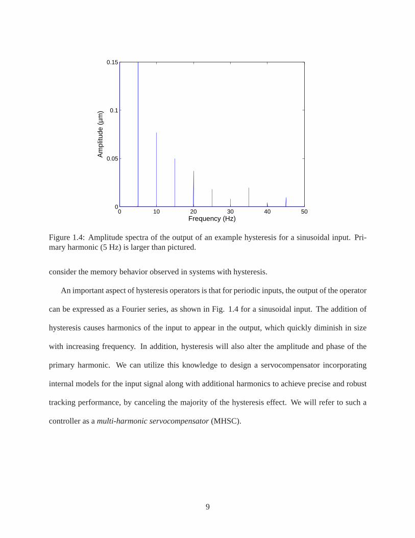
Figure 1.4 Amplitude spectra of the output of an example hysteresis for a sinusoidalinput. Primary harmonic (5 Hz) is larger than pictured. . . . .. . . . . . 9
Figure 2.1 Illustration of a Play Operator.r is the play radius. . . . . . . . . . . . . . 15
Figure 2.2 The inversion process for hysteresis operators.ud is the desired output,andu is the actual output. . . . . . . . . . . . . . . . . . . . . . . . . . . 17
Figure 2.3 Deadzone functions with positive and negative thresholds. The slopes inlinear regions are unity. . . . . . . . . . . . . . . . . . . . . . . . . . . . 19
Figure 2.4 Illustration of the PKP hysteron. This operator is parameterized by thethresholdsα, β , and slopea. . . . . . . . . . . . . . . . . . . . . . . . . 24
Figure 3.1 Closed-loop system with hysteresis, as defined in (3.13), (3.14), and (2.27). 31
Figure 3.2 Equivalent block diagram for the closed-loop system (2.13),(3.13), and(3.14) in steady state analysis. . . . . . . . . . . . . . . . . . . . . . . .34
Figure 3.3 Nanopositioning stage used in experimentation, Nano-OP65 nanopositioningstage coupled with a Nano-Drive controller from Mad City Labs Inc, with a pri-mary resonance of 3 kHz. Position feedback is provided by a built-in capacitivesensor. . . . . . . . . . . . . . . . . . . . . . . . . . . . . . . . . . . . . 37
Figure 3.4 Measured hysteresis loops for the nanopositioner. . . . . . . . . . . . . . 38
Figure 3.5 Plant output used in the identification of the modified PI operator, andresulting model output. . . . . . . . . . . . . . . . . . . . . . . . . . . . 39
ix

Figure 3.6 Model prediction and experimental data for a decreasing sinusoid used tooptimize the hysteresis model. . . . . . . . . . . . . . . . . . . . . . . . 39
Figure 3.7 Experimental results at 200 Hz for the proposed methods (SHSC andMHSC), ILC and PI+I. . . . . . . . . . . . . . . . . . . . . . . . . . . . 42
Figure 3.8 Comparison between multi-harmonic servocompensator (MHSC) and It-erative Learning Control (ILC). . . . . . . . . . . . . . . . . . . . . . . . 43
Figure 3.9 Frequency spectra of the tracking error signal for references at 5 Hz and200 Hz. An SHSC was used in each case. Graphs are aligned so that thepeaks on each graph correspond to the same harmonic of the reference.Note the prominence of the harmonics near 3000 Hz in the 200 Hzplot. . 44
Figure 3.10 Experimental results at 50 Hz for sawtooth reference signal. Two periodsare shown. . . . . . . . . . . . . . . . . . . . . . . . . . . . . . . . . . . 46
Figure 3.11 Experimental results for a reference trajectory of yr = 5sin(2π5t−π/2)+5sin(2π15t +π/2)+10sin(2π25t −π/2) . . . . . . . . . . . . . . . . . 47
Figure 3.12 Tracking errors for a 50 Hz reference signal, forloaded and unloadednanopositioner. An MHSC was used in both cases. Note the similarity inthe time trajectory of the tracking error. . . . . . . . . . . . . . . .. . . 48
Figure 4.1 A sample curve showing how the time instantsTi andTo are calculatedfor a play operator. The variabler is the radius of the play operator, andit is assumed that the input at time zero is 2r. . . . . . . . . . . . . . . . . 53
Figure 4.2 Reconstruction of the outputu(t) of a play operator. The play radiusr = 0.3, and the time axis is shared by each signal. . . . . . . . . . . . . . 54
Figure 4.3 Plot ofcn for increasing amplitudeA. The play radius is held constant atr = 0.5. . . . . . . . . . . . . . . . . . . . . . . . . . . . . . . . . . . . 58
Figure 4.4 Plot ofcn for increasing play radiusr. Values ofcn andr are normalizedby the input amplitudeA. . . . . . . . . . . . . . . . . . . . . . . . . . . 59
Figure 4.5 Mean tracking errors for various controllers andplay radii. Note that thecontroller gains and structure is unchanged by altering theplay radius. . . 65
Figure 5.1 Tracking error for a 50 Hz reference signal, with two periods shown.Tracking range is± 20 µm. . . . . . . . . . . . . . . . . . . . . . . . . . 83
x

Figure 5.2 Tracking error for a 200 Hz reference signal with four periods shown.Tracking range is± 20 µm. . . . . . . . . . . . . . . . . . . . . . . . . . 83
Figure 5.3 Tracking error under a changing reference signal. . . . . . . . . . . . . . 86
Figure 5.4 Trajectory ofψ(1) under a changing reference signal. . . . . . . . . . . . 86
Figure 5.5 Experimental results for adaptive servocompensator implemented withfour adaptation variables.ψ(1) andψ(3) are shown in the top plot. No-tice the peaking events in the adaptation variables near 30 and 42 s. Thelower plot shows the tracking error during the second peaking event. . . . 88
Figure 6.1 Block Diagram of the closed-loop system. . . . . . . . .. . . . . . . . . 93
Figure 6.2 Phase portrait of average system for a sample plant and controller. Thezero level curves ofθ1 (primarily vertical) andθ1 (primarily horizontal)together with the neutral axisθ1 = θ2 are also plotted. . . . . . . . . . . . 110
Figure 6.3 Illustration of linear plant preceded by hysteresis operator, commonlyused to model piezoelectric-actuated nanopositioners. . .. . . . . . . . . 110
Figure 6.4 Simulation results on the model of the piezoelectric plant. Two simula-tions are presented, withR11 = 10 andR11 = 11. . . . . . . . . . . . . . . 115
Figure 6.5 Output spectrum for nanopositioner used in experimental studies. Inputto power supply is 3sin(2π5)+4V. Primary harmonic is not shown, buthas an amplitude of 25.2 µm. . . . . . . . . . . . . . . . . . . . . . . . . 115
Figure 6.6 Experimental results for a 5 Hz sinusoidal signal. . . . . . . . . . . . . . 118
Figure 6.7 Experimental results for a 100 Hz sinusoidal signal. . . . . . . . . . . . . 118
Figure 6.8 Experimental Results for a 5 Hz sawtooth signal. . .. . . . . . . . . . . 119
Figure 6.9 Phase portrait ofσ1 andσ2 for various initial conditions. Desired equi-libria are marked by the stars (red, in the lower right and topleft), andinitial conditions are marked by squares. . . . . . . . . . . . . . . .. . . 120
Figure 6.10 Plot of tracking error and adaptation variablesvs. time. Adaptation isenabled at 2 s. . . . . . . . . . . . . . . . . . . . . . . . . . . . . . . . . 120
xi

Figure 6.11 Phase portrait for experiments withσ1(0) = σ2(0) = 2π50 andσ1(0) 6=σ2(0) (σ1(0) = 2π50,σ2(0) = 2.01π50.) . . . . . . . . . . . . . . . . . 121
Figure 7.1 Hysteresis loops for play operators with equalized relative gains, whereris equal to 0.7, andµ = 3. . . . . . . . . . . . . . . . . . . . . . . . . . . 139
Figure 7.2 Mean tracking error for controllers used in experimental trials. SHSCrefers to compensation of only the reference harmonic, and MHSC refersto compensation of the first, second, and third harmonics of the reference. 144
Figure 7.3 Frequency spectrum of the tracking error with SHSC with and without in-version. Bump near 3 kHz is caused by the resonance peak of the nanopo-sitioner. . . . . . . . . . . . . . . . . . . . . . . . . . . . . . . . . . . . 145
Figure 8.1 Hysteresis state for systems that are unstable when the hysteresis is in theplay region, with varying play radii. . . . . . . . . . . . . . . . . . . .. 150
Figure 8.2 Closed-loop system described in (8.5). . . . . . . . . .. . . . . . . . . . 150
Figure 8.3 Illustration of the state of the play operatorPr during a sine-like limitcycle. The stars indicate times when the system dynamics switch. . . . . . 153
Figure 8.4 Switching times computed from algorithm and simulation, versus gainkp. 165
Figure 8.5 Limit cycle solutions computed from algorithm and simulation, versusgainkp. . . . . . . . . . . . . . . . . . . . . . . . . . . . . . . . . . . . 166
Figure 8.6 Peak amplitude of limit cycles versus absolute value of the limit cyclesolutionsα0. . . . . . . . . . . . . . . . . . . . . . . . . . . . . . . . . . 167
Figure 8.7 True solution and Scaled solution forr = 1. Note the phase differencecreated by the different transient behavior. . . . . . . . . . . . .. . . . . 168
Figure 8.8 True solution and Scaled solution forr = 1 at steady state, with phaseoffset included. . . . . . . . . . . . . . . . . . . . . . . . . . . . . . . . 169
Figure 8.9 True solution and Scaled solution fora = 10 at steady state, with phaseoffset included. . . . . . . . . . . . . . . . . . . . . . . . . . . . . . . . 169
xii

Chapter 1
Introduction
1.1 Systems with Hysteresis
The phenomenon hysteresis is caused by the existence of multiple possible internal states within a
system for a given input. This phenomenon was first observed by scientists in the fields of ferro-
magnetism [3] and plasticity [1] in the late 19th century, shown in Fig. 1.1. Mathematical models
of hysteresis were first developed by Preisach [4] and Prandtl [5] in the early 20th century. Most
research on hysteresis focused on modeling and characterization of physical hysteresis until the
1970’s, when the mathematical theory of ordinary differential equations coupled with hysteresis
operators was developed [6,7]. Recent advances in the field ofmaterials science have created a new
class of actuator/sensor hybrids calledSmart Materials[8], whose behavior strongly exhibits hys-
teresis. A broad range of materials fall into this class, including piezoelectrics [9], shape memory
alloys [10], electro-active polymers [11], magnetostrictives [12], magnetorheological fluids [13],
and conjugated polymers [14]. Piezoelectric materials were the first of these smart materials to be
developed, with the discovery of the piezoelectric coupling effect in the 1800’s [9], and have been
successively employed in a variety of industries includingmanufacturing, automotive, and medical
devices [15].
Of particular importance to our work is the technology of nanopositioning, which deals with
precision motion and manipulation on the nanometer scale. Nanopositioning plays a key role in
technologies like Scanning Probe Microscopy (SPM), used inthe advancement of fields such as
1
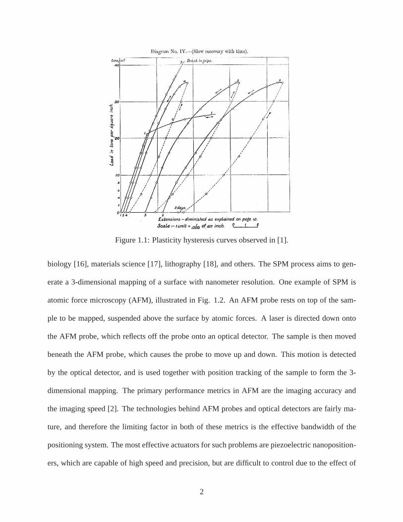
Figure 1.1: Plasticity hysteresis curves observed in [1].
biology [16], materials science [17], lithography [18], and others. The SPM process aims to gen-
erate a 3-dimensional mapping of a surface with nanometer resolution. One example of SPM is
atomic force microscopy (AFM), illustrated in Fig. 1.2. An AFM probe rests on top of the sam-
ple to be mapped, suspended above the surface by atomic forces. A laser is directed down onto
the AFM probe, which reflects off the probe onto an optical detector. The sample is then moved
beneath the AFM probe, which causes the probe to move up and down. This motion is detected
by the optical detector, and is used together with position tracking of the sample to form the 3-
dimensional mapping. The primary performance metrics in AFM are the imaging accuracy and
the imaging speed [2]. The technologies behind AFM probes and optical detectors are fairly ma-
ture, and therefore the limiting factor in both of these metrics is the effective bandwidth of the
positioning system. The most effective actuators for such problems are piezoelectric nanoposition-
ers, which are capable of high speed and precision, but are difficult to control due to the effect of
2

Figure 1.2: Illustration of Atomic Force Microscopy from [2].
hysteresis.
The promising applications of smart materials have motivated efforts to better understand and
control their behavior, which has ignited further researchinto systems with hysteresis. When mod-
eling the behavior of smart materials, it is important to distinguish between sensing and actuation
models. Modeling conducted for sensing applications typically focuses on the internal dynamics
of the smart materials, and are often based on the physics andchemistry of the materials [19–21].
In modeling the actuation behavior of smart materials, a more phenomenological or “Black box”
approach can be taken. A common and faithful model for smart material actuators consists of a
linear system preceded by a hysteresis operator [11,22–26]:
x(t) =Ax(t)+Bu(t)
u(t) =Γ[v;Γ0](t) (1.1)
wherev(t) is the system input, andΓ is a hysteresis operator [7, 27–29]. It is also worth noting
that there are significant uncertainties in both the hysteresis and dynamics of the system, as the
3

(a) Relay hysteron
+1
v
–1 a
u
(b) PKP hysteron (c) Play hysteron
Figure 1.3: Hysterons of several Presiach-like operators.For interpretation of the references tocolor in this and all other figures, the reader is referred to the electronic version of this dissertation.
behavior of the system varies with environmental and loading conditions [2]. We will refer to
this combination of a linear dynamic system and hysteresis operator as asystem with hysteresis.
Clearly, in order to control the actuation of smart materials, we must investigate such systems with
hysteresis.
The first step in our investigation is to identify the system model (1.1) to be considered. As
there are a wealth of tools available for capturing linear dynamics, most research into the modeling
of systems with hysteresis is focused on characterization and identification of the hysteresis opera-
tor. The oldest and most widely used is the Preisach model [4], developed in the 1930’s as a model
for magnetic hysteresis. Presiach models are formed through a weighted superposition of relay
hysterons(shown in Fig. 1.3a), unit hysteresis elements whose parameters are varied to approxi-
mate a wide variety of physical hysteresis phenomena [8,28]. The Preisach model has also proven
to be an excellent model for smart material actuators [25,30,31]. As the effectiveness of the opera-
tor itself is fairly established, most recent works have focused on identification or implementation
of the Presiach operator [12,23].
The success and maturity of the Preisach model has resulted in the development of a number
of “Preisach-like” operators [22], which use hysterons modified from the original Preisach model.
4

The Preisach-Krasnosel’skii-Pokrovskii (PKP) operator [24, 29] is formed with PKP hysterons
(Fig. 1.3b), which are similar to the relay hysteron but incorporate finite slopes. In our work,
we will focus on the Prandtl-Ishlinskii (PI) operator [5], which uses play operators as hysterons
(Fig. 1.3c), in reference to the phenomenon of mechanical play they emulate. We will also make
use of the modified PI operator [32], which consists of a PI operator cascaded with dead-zone
operators. As we will see in Chapter 2, the PI operator and its generalization possesses several
practical advantages over other Preisach-like operators that make it well suited for online control
applications.
1.2 Control of Systems with Hysteresis: Existing work
Once we have arrived at a faithful model for a system with hysteresis, we can then address the
problem of controller design for such systems. A common control objective for any actuator is to
force the trajectory of the system to track a desired reference. This is also the case in nanoposition-
ing applications like SPM, where the positioner output is intended to track a predescribed path. A
multitude of control strategies have been proposed to solvesuch tracking problems in systems with
hysteresis [33–39]. As with modeling systems with hysteresis, the meritorious element of these
controllers is the manner in which they address the effect ofhysteresis within the system. For
most of these controller designs, we can differentiate between their philosophies as being either
inversion-focused or rejection-focused. The differencesbetween these control techniques are often
closely tied to the system model considered by the authors.
5

1.2.1 Inversion-Focused Methods
One of the most natural and widespread approaches in controltheory is the technique of model
inversion. The objective of model inversion is to design a controller to reduce the input-output map
of a system to a unity gain. Following the development of hysteresis models, researchers began
to develop inverse hysteresis operators for use in control applications. Inversion strategies for
the Preisach operator have been developed [23, 31, 40]; however, these result in only approximate
inversions. The PI operator on the other hand possesses a closed-form inversion [32], which turns
out to be another PI operator. For both models, hysteresis inversion has proven to be a very effective
technique for reducing the impact of hysteresis, and it is commonly used in the control of systems
with hysteresis [12,22,23,33,34,40–42].
Inversion-focused control algorithms center around improving or optimizing a hysteresis in-
version, often through online adaptation of the weights of aPreisach-like operator. This approach
was first detailed in [33], where an adaptive inverse approach based on a generic hysteresis model
and model reference adaptive control (MRAC) was proposed. An obstacle to this design is that
classical MRAC approaches, such as those described in [43], lead to bilinear coupling of adapta-
tion terms. Such bilinear coupling impedes the design of adaptation laws unless one of the coupled
terms is a scalar [43]. This was addressed in [33] through over-parameterization of the adapta-
tion variables. In [41], slow adaptation was utilized in an MRAC scheme to separate adaptation
of the hysteresis parameters from the controller parameters. An adaptive sliding mode approach
coupled with adaptive hysteresis inversion was used in [44]for discrete-time systems with hystere-
sis. In addition, neural networks have been used to invert hysteresis and compensate for uncertain
dynamics [45].
A noteworthy disadvantage of these methods is that the high numbers of hysterons required by
6

Presiach-like operators makes these adaptive approaches computationally expensive. For example,
55 hysterons were used to describe the hysteresis behavior of a magnetostrictive material in [35],
which, if used in an inversion-focused control strategy, would require implementation of 55 on-
line adaptation laws. In addition, implementation of the inversion itself can be computationally
expensive, a fact that we will observe in Chapter 7. These computational concerns have motivated
efforts to implement hysteresis inversions using an FPGA [46]; however, this adds another level of
complexity to the design and analysis of the system.
1.2.2 Rejection-Focused Methods
An alternate way of thinking, as opposed to the inversion-focused approach, is to consider the
undesirable effects of hysteresis as an uncertain disturbance to be rejected. The hysteresis effect
is broken into a known gain and an uncertain disturbance, andthe controller is then designed to
be robust to the uncertainty. This technique is especially popular in the nanopositioning literature,
where the high performance demands of SPM systems require controllers capable of tracking and
disturbance attenuation.H∞ control [37] and 2-degree of freedom control [47] have been shown to
provide robustness to plant uncertainty and facilitate tracking in the presence of hysteresis. A sim-
ilar approach was used in [48], where a high gain and notch filter feedback controller is combined
with a feedforward dynamic inversion. In the work of [49], the hysteresis effect was modeled by
a combination of a linear gain and unstructured exogenous disturbance, which is attenuated by an
adaptive robust controller. Sliding mode control [39] and disturbance observers [50,51] have also
been used to compensate for the effect of hysteresis.
The stability proofs in these papers are carried out using the ubiquitous Lyapunov criterion.
However, by assuming the hysteresis to be an unstructured disturbance, these methods ignore the
operator behavior of the hysteresis, and therefore can onlyprove ultimate boundedness of the
7

states. Indeed, later in this dissertation we will also showthat using such design methods can
cause the controller to send the system into a self-excited limit cycle. In addition, the theoretical
bounds on the tracking error can be very conservative, a factthat has motivated efforts to improve
the accuracy of the model bounds [52].
1.3 The Multi-Harmonic Servocompensator: Union of Design
Philosophies
As we have discussed, inversion-focused and rejection-focused methods are fundamentally op-
posed in the mindset behind their designs. Inversion-focused methods use detailed modeling of
the hysteresis phenomenon in order to achieve robust performance, but suffer from the resulting
controller complexity. Rejection-focused methods utilizethe might of control theory to attenu-
ate the effect of hysteresis, without explicitly utilizingknowledge of the phenomenon itself in the
controller design. In a union of these philosophies, we willexplore the use ofservocompensators
in systems with hysteresis. We will see that the design of this servocompensator makes specific
use of the effect of hysteresis in the closed-loop system to formulate asimple, robust, andhigh-
performancecontroller for systems with hysteresis.
Servocompensators, also referred to as internal-model controllers, were originally designed in
the 1970’s by Davison [53, 54] and Francis [55, 56]. The defining feature of servocompensators
is their ability to completely cancel signals contained within the design class of their internal
models. This property is also shown to be robust to perturbations from both exogenous inputs
and model uncertainties, as long as the system is not destabilized. This makes servocompensators
excellent choices for solving tracking problems. Isidori and Byrnes [57] extended the internal
model approach to nonlinear systems; however, the class of nonlinear systems considered does not
8
0 10 20 30 40 500
0.05
0.1
0.15
Frequency (Hz)
Am
plitu
de (
µm)
Figure 1.4: Amplitude spectra of the output of an example hysteresis for a sinusoidal input. Pri-mary harmonic (5 Hz) is larger than pictured.
consider the memory behavior observed in systems with hysteresis.
An important aspect of hysteresis operators is that for periodic inputs, the output of the operator
can be expressed as a Fourier series, as shown in Fig. 1.4 for asinusoidal input. The addition of
hysteresis causes harmonics of the input to appear in the output, which quickly diminish in size
with increasing frequency. In addition, hysteresis will also alter the amplitude and phase of the
primary harmonic. We can utilize this knowledge to design a servocompensator incorporating
internal models for the input signal along with additional harmonics to achieve precise and robust
tracking performance, by canceling the majority of the hysteresis effect. We will refer to such a
controller as amulti-harmonic servocompensator(MHSC).
9

1.4 Overview of Contributions
The principle contribution of this work lies in addressing the tracking problem for systems with
hysteresis using servocompensators, which we approach in several ways. We first discuss the de-
sign and analysis of a servocompensator for solving tracking problems in systems with hysteresis,
which we validate experimentally through implementation on a commercial nanopositioning stage.
A crucial element of this analysis is that we utilize a modified PI operator to model the hysteresis in
the system. This operator possesses an important contraction property, which, coupled with an ap-
proximate hysteresis inversion, allows us to prove the existence of a unique, asymptotically stable,
periodic solution. We can then invoke the disturbance rejection properties of the servocompensator
to prove the attenuation of hysteresis at steady state, assuming that the internal model of the desired
reference trajectory is known. Our experimental results will confirm the rejection properties of the
controller, where we show our proposed method can achieve one third of the mean tracking error
of a competitive technique in nanopositioning (Iterative Learning Control).
We then present results on a tool for computing the output of ahysteresis operator are pre-
sented, based on Fourier series theory. This algorithm firstformulates the output of individual
hysterons as a series of pulse signals in combination with the input, which facilitate evaluation
of the Fourier integrals. Then, by assuming either a sinusoidal or sawtooth input signal, we will
show that the Fourier coefficients can be computed in a closedform manner. We then present sim-
ulation results on this method, and show that the algorithm represents a valuable design tool for
servocompensators in systems with hysteresis.
Next, we will extend the design of the MHSC to cases where the internal model of the reference
is not knowna priori. We first adapt a traditionally designed nonlinear adaptiveservocompensator,
and prove its stability in systems with hysteresis. This approach combines high-gain stabilizing
10

control with a canonical internal model controller that is subject to adaptation. During our discus-
sion of the experimental results, we will discover that thisdesign cannot incorporate the principles
of the multi-harmonic servocompensator to reduce the effect of hysteresis. We will then discuss the
inclusion of a frequency estimator based on slow adaptationinto the MHSC, a design which we re-
fer to as anindirect adaptive servocompensator(IASC). In this discussion, the term frequency will
to the fundamental frequency of a periodic signal. For example, a sinusoid, a triangular wave, or a
square wave will all be described as having one frequency although the latter two clearly have har-
monic frequency components. However, these harmonics are known multiples of the fundamental
frequency; therefore knowledge of the fundamental frequency implies knowledge of the remaining
harmonic components. Through our stability analysis, we will analytically demonstrate some note-
worthy properties for systems with one, two, andn unknown frequencies. In particular, for systems
with one unknown frequency, we will prove and verify a stability condition related to the amplitude
of the reference signal as compared to disturbances, and forthe case of two unknown frequencies,
prove the existence of a degenerate case for the system. We will then prove the stability of such
controllers in a system with hysteresis, and demonstrate its performance experimentally.
Next, we discuss the stability and tracking error convergence of a system with hysteresis using a
general feedback controller with an integral action. The theory of switched systems, in particular,
that of the common Lyapunov function [58], and a linear matrix inequality (LMI) will be used
to prove that the tracking error and state vector exponentially converge to zero for a constant
reference. The principal contribution of this work is to present sufficient conditions (in the form
of an LMI) for the regulation of the closed-loop system in terms of the hysteresis parameters,
without requiring the hysteresis to be small. This addresses a key weakness of our prior results,
namely the requirement that hysteresis inversion be included in the controller design in order to
prove stability. As we will see, the presence of an integral action is crucial to the formulation of
11

our LMI condition. This then allows us to show the stability of systems with hysteresis controlled
by servocompensators without requiring hysteresis inversion. We then show that the MHSC can
achieve even higher performance without hysteresis inversion than when hysteresis inversion is
used; in particular, the mean tracking error achieved by theMHSC is cut in half when hysteresis
inversion is removed.
Finally, inspired by discoveries made during the course of the LMI work, we investigate self-
excited limit cycles occurring in a particular class of systems with hysteresis. In particular, we will
focus on a linear plant controlled by an integral controller, where a play operator [32] is present
in the feedback loop. We focus our attention on odd symmetriclimit cycles within the system. A
Newton-Raphson algorithm is formulated to calculate the limit cycles, and using the odd symmetry,
we are then able to prove that there exist linear relationships between several properties of the limit
cycles and the parameters of the system. These results are verified in simulation, where we also
demonstrate the effectiveness of the Newton-Raphson algorithm at predicting the solutions of the
system. We will also illustrate a crucial weakness of rejection-focused designs, in that even for
constant references, the steady-state trajectory may be a self-excited limit cycle.
The dissertation is organized as follows. Chapter 2 providesbackground information on the
hysteresis models used in this work. We also derive some important expressions used in the anal-
ysis of the closed-loop systems with hysteresis in the following Chapters. Chapter 3 presents the
design and analysis of our proposed MHSC in systems with hysteresis, as well as experimental
comparisons to established control methods. Our Fourier series algorithm is contained in Chapter
4. We investigate the application of a traditional adaptiveservocompensator to nanopositioning
control in Chapter 5, which also motivates the design of our novel adaptive servocompensator.
Chapter 6 discusses the design, analysis, and experimental validation of the proposed IASC. The
LMI results proving stability of our controller without using hysteresis inversion are contained in
12

Chapter 7. Our limit cycle investigation is contained in Chapter 8. Finally, we provide concluding
remarks and discuss potential future work in Chapter 9.
13

Chapter 2
Overview of Hysteresis Models
2.1 Introduction
As we have discussed in Chapter 1, the primary challenge in modeling of systems with hysteresis
is the formulation of the hysteresis operator. A complete review of hysteresis modeling is outside
the scope of this dissertation; we instead direct the readerto the monographs [7, 28, 29] for such
an overview. We will instead focus on the operators used within this thesis; the Prandtl-Ishlinskii
(PI) operator, modified Prandtl-Ishlinskii (modified PI) operator, and the Preisach-Krasnosel’skii-
Pokrovskii (PKP) operator. Each operator falls under the umbrella of “Presiach-Like” operators
described in Section 1.2, in that each is formed by a weightedsuperposition of unit hysteresis
elements called hysterons. We will begin the discussion of each hysteresis operator by presenting
the details of its hysteron, followed by the formulation of the operator itself. In addition, we will
also discuss inversion of the PI and modified PI operators, and characterize the inversion error
when the inversion is inexact.
2.2 The Prandtl-Ishlinskii Operator
The PI operator has seen widespread use in modeling piezoelectric hysteresis [26, 32, 44, 59]. In
this dissertation, we will focus on the PI operator because it possesses a variety of of important
mathematical properties which are useful to control designers. First, the PI operator possesses an
14

exact, closed form inversion, which makes the operator an excellent choice for control designers
interested in online implementation. Second, it possessesa contraction property which, as we will
see, can be utilized in the stability proofs of several closed-loop systems considered in this thesis.
The hysteron of the PI operator is the play operator, illustrated in Fig. 2.1. The play operator
is characterized by a single parameterr i, which we refer to as the play radius. For a monotone
continuous inputv(t), we denote the output and state of a play operator with radiusr i as
Pr i [v;Pr i [v](0)](t) = maxminv(t)+ r i ,Pr i [v](0),v(t)− r i (2.1)
By breaking any arbitrary input into monotone segments and replacingPr i [v](0) by Pr i [v](ti), where
the monotonicity ofv(t) changes atv(ti), the statePr i [v](t) can be defined for arbitrary inputs.
Figure 2.1: Illustration of a Play Operator.r is the play radius.
Now define the vectorsr = [r0, r1, · · · , rp]′ andθh = [θh0,θh1, · · · ,θhp]
′, where′ denotes the
transpose. The PI operator, which we will denote asΓh, is written as
Γh[v;W(0)](t) =p
∑i=0
θhiPr i [v;Pr i(0)](t) (2.2)
where we let the vectorW(t) = [W0(t),W1(t), · · · ,Wp(t)]′ represent the states of the play operators
15

(i.e. Wi(t) = Pr i [v;Pr i(0)](t)). We can also writeΓh in the inner product form
Γh[v;W(0)](t) = θ ′hW(t) (2.3)
For later use, we will also define the operatorP, which captures the evolution ofW(t) under the
inputv(t);
W(t) = P[v;W(0)](t) (2.4)
Remark 1 The PI operator described in Eqs.(2.2)-(2.4) is also referred to as a finite-element PI
operator. A more accurate description of hysteresis can be achieved by using an infinite-element PI
operator [32, 44]. However, in the interest of practical application, the finite-element PI operator
is often used in controller design. Therefore, we focus on thefinite-element PI operator in this
thesis.
We now discuss the inversion of the PI operatorΓh. Specifically, we will discuss the formula-
tion of the left inverse of the PI operatorΓh, which we will define asΓ−1h . This inverse operator is
also a PI operator, with different weights and initial conditions. Let ¯r andθh denote the radius and
weights of the play operators of the inverse operator. Then we can write the inverse operator, with
inputud(t), as
Γ−1h [ud;W(0)](t) =
p
∑i=0
θhiPr i [ud; Pr i(0)](t) (2.5)
where we have denoted the state of the play operators inΓ−1h with the vector
W(t) = [W0(t),W1(t), · · · ,Wp(t)]
The inverse parameters ¯r, θh, andW(0) can be calculated from the following equations, presented
16

in [32]:
r i =i
∑j=0
θh j(r j − r i), i = 0,1, · · · , p (2.6)
θh0 = 1/θh0 (2.7)
θhi =− θhi(θh0+∑i
j=1θh j
)(θh0+∑i−1
j=1θh j
) , i = 1, · · · , p (2.8)
Wi(0) =i
∑j=0
θh jWi(0)+p
∑j=i+1
θh jWj(0), i = 0,1, · · · , p (2.9)
Figure 2.2: The inversion process for hysteresis operators. ud is the desired output, andu is theactual output.
The inversion process is illustrated in Fig. 2.2. The inversion inputud(t) is the desired output
of the hysteresis operator, and is designed to accomplish some larger control objective, such as
tracking or stabilization via state feedback. As the hysteresis operator is modeled as part of the
plant itself,v(t) is the input to the hysteretic system. The signalu(t) is the output of the modeled
hysteresis operator in the plant, and therefore is not measurable or available for use in the controller.
However, its definition is very useful in analysis of the system.
The inverse operatorΓ−1h is an exact inversion, implying that the difference betweenu andud
is identically zero. However, in practical circumstances the forward hysteresis operatorΓh is not
exactly known. Rather, only an estimateΓh, with weightsθh and radii ˆr, is available for control
17

design. In our work, we will operate under the following assumption.
Assumption 1 The uncertainty between the modelsΓh andΓh is limited to the weightsθh andθh.
This implies thatr = r is known.
This assumption is commonly used by designers working with the PI model [32], as the radii are
chosen to span the available input range of the actuator, andthe order of the model is chosen
based on computational concerns. This approximate model and its parameters are used to create
the approximate inversion,Γ−1h , whose weights and radii areθh and ¯r. We will now replace the
ideal inversionΓ−1h with this approximate inversion. With the input ofud and output ofv, the
approximate inversion obeys the equation
v(t) = Γ−1h [ud;W(0)](t) =
p
∑i=0
¯θhiPr i[ud; Pr i
(0)](t) (2.10)
We will now characterize the inversion erroru(t)−ud(t) when an approximate inversion is used.
u(t) is still described by (2.3). Since the PI operator’s inversion is exact, we can use (2.10) to write
ud(t) as
ud(t) =Γh[Γ−1
h [ud;W(0)];W(0)](t)
=Γh[v;W(0)](t), θ ′hW(t) (2.11)
Using (2.3) and (2.11), we can then write
ud(t)−u(t) = θ ′hW(t)−θ ′
hW(t), θ ′hW(t) (2.12)
18

whereW(t) is defined by composite hysteresis operator
W(t) = W [ud;W(0)](t), P Γ−1h [ud;W(0)](t) (2.13)
2.3 Modified Prandtl-Ishlinskii Operator
A disadvantage of the PI operator is that it is odd symmetric,which can be seen from the illustration
of the play operator in Fig. 2.1. This is a significant disadvantage, as the hysteresis loops exhibited
by smart material systems are often asymmetric. In [32], a modified PI operator was proposed
to address this deficiency. This model combines the originalPI operator with a superposition of
one-sided deadzone functions, illustrated in Fig 2.3. Eachdeadzone function is parameterized by
a single threshold parameter, written asz in Fig. 2.3. The output a deadzone functiondzi , wherezi
is the threshold, can be expressed as
(a) Negative threshold. (b) Positive threshold.
Figure 2.3: Deadzone functions with positive and negative thresholds. The slopes in linear regionsare unity.
19

dzi(v(t)) =
max(v(t)−zi ,0), zi > 0
v(t), zi = 0
min(v(t)−zi ,0), zi < 0
(2.14)
Note that ifzi = 0, the deadzone function becomes a unity gain. Now denote thevector of deadzone
thresholdsz= [z−l , · · · ,z−1,z0,z1, · · · ,zl ]′, where
−∞ < z−l < · · ·< z−1 < z0 = 0< z1 < · · ·< zl < ∞
We will also denote the weight vectorθd = [θd−l , · · · ,θd−1,θd0,θd1, · · · ,θdl ]′. We can now denote
the superposition of deadzone functions asΦ, with inputv1(t) as
Φ(v1(t)) =l
∑i=−l
θdidzi(v1(t)), θ ′dDz(v1(t)) (2.15)
where the vectorDz(v(t)) = [dz−l (v(t)), · · · ,dzl (v(t))]′ denotes a stack of deadzone functions with
thresholdsz. Using (2.15) along with (2.3), we can define the modified PI operator, denoted as
Γhd. With inputv(t), the operator can be written as
Γhd[v;W(0)](t) = Φ(Γh[v;W(0)](t)) = θ ′dDz(θ ′
hW(t)) (2.16)
As the deadzone operator is simply a collection of functions, a closed form inversion also exists
for the deadzone operator. This inversion is also a deadzoneoperator, with modified weights and
thresholds. For deadzone functions with positive thresholds, the inversion parametersθd andzcan
20

be computed as
zi =i
∑j=0
θd j(zj −zi), i = 0, · · · , l (2.17)
θd0 = 1/θd0 (2.18)
θdi =− θdi(θd0+∑i
j=1θd j
)(θd0+∑i−1
j=1θd j
) , i = 1, · · · , l (2.19)
and for negative thresholds,
zi =0
∑j=i
θd j(zj −zi), i =−l , · · · ,0 (2.20)
θd0 = 1/θd0 (2.21)
θi =− θdi(θd0+∑−1
j=i θd j
)(θd0+∑−1
j=i+1θd j
) , i =−l , · · · ,0 (2.22)
Using these definitions, we can form the inverse of the modified PI operator as
Γ−1hd [ud;W(0)](t) = Γ−1
h [θ ′dDz(ud);W(0)](t) (2.23)
Note that the order of the PI and deadzone operators are switched in the inverse operator with
respect to the forward operator. We have already discussed how the hysteresis models are unknown
in practical applications. Therefore, we must consider an inexact hysteresis inversion, based on an
approximation ofΓhd, which we denote asΓhd.
Assumption 2 The uncertainty between the modelsΓhd and Γhd are limited to the hysteresis
weightsθh and θh, and the deadzone weightsθd and θd. This implies that the vectors r and z
are known.
21

This is a similar condition to that imposed for the PI operator in Assumption 1, and it is made for
similar reasons. We will denote this estimate and its outputu(t) as
u(t) = Γhd[v;W(0)](t) = Φ(Γh[v;W(0)](t)) = θ ′dDz(θ ′
hW(t)) (2.24)
We can then use the approximated model to derive an approximate inversion,
Γ−1hd [ud;W(0)](t) = Γ−1
h [ ¯θ ′dD¯z(ud);W(0)](t) (2.25)
Our final discussion regarding the modified PI operator considers the inversion error, where we
attempt to derive a similar expression for the inversion error as that achieved for the PI operator in
(2.12). Using the identityud(t) = Γhd[Γ−1hd [ud;W(0)];W(0)] and (2.24), the inversion erroru(t)−
ud(t) can be expressed as
ud(t)−u(t) = θ ′dDz(θ ′W(t))−θ ′
dDz(θ ′W(t)) (2.26)
whereW(t) is defined by the composite hysteresis operator
W(t) = Wd[ud;W(0)](t), P Γ−1hd [ud;W(0)](t) (2.27)
We will now derive a bound for this inversion related to the parameter errors, which we define as
θd = θd −θd andθh, defined in (2.12). Adding and subtractingθ ′dDz(θ ′
hW(t)) to (2.26) allows us
22

to arrive at
ud(t)−u(t) =θ ′dDz(θ ′
hW(t))−θ ′dDz(θ ′
hW(t))+ θ ′dDz(θ ′
hW(t))− θ ′dDz(θ ′
hW(t))
=(θ ′d −θ ′
d)Dz(θ ′W(t))+ θ ′d[Dz(θ ′
hW(t))−Dz(θ ′hW(t))] (2.28)
It can be easily seen from (2.14) that the dead-zone operatorobeys the Lipschitz condition
|dzi(a)−dzi(b)| ≤ |a−b| (2.29)
for any thresholdzi. Using this property together with the holder inequality, and taking the absolute
value of (2.28), we have
|u−ud| ≤‖θd‖‖Dz(θ ′hW(t))‖+‖θd‖∞[(2l +1)|θ ′
hW(t)|]
≤‖θd‖‖Dz(θ ′hW(t))‖+‖θd‖∞[(2l +1)‖θh‖‖W(t)‖]
≤εd[‖Dz(θ ′hW(t))‖+(2l +1)‖θd‖∞‖W(t)‖] (2.30)
whereεd = max(‖θh‖,‖θd‖) and‖ · ‖∞ represents the infinity norm [60].
2.4 The Preisach-Krasnosel’skii-Pokrovskii Operator
The final hysteresis operator we will address is the Preisach-Krasnosel’skii-Pokrovskii, or PKP
operator [24,29,61]. We will not be utilizing this model in any experiments, and therefore we will
not be discussing the inversion of this operator. The PKP hysteron is defined by three parameters,
labeled in Fig. 2.4 asα, β , anda. This hysteron is very similar to the Preisach hysteron (therelay
operator); however, the inclusion of the slope parametera allows for a continuous output with a
23

+1
v
–1 a
u
Figure 2.4: Illustration of the PKP hysteron. This operatoris parameterized by the thresholdsα,β , and slopea.
finite number of hysterons. The selections ofα andβ allow the operator to model hysteresis curves
of complex shapes. For a monotone continuous inputv(t), the output of the PKP hysteron can be
described by
u(t) =
min(maxv(0),−1+ 2(v(t)−α)a ,−1,1) for v≥ 0
max(minv(0),−1+ 2(v(t)−β )a ,−1,−1) for v≤ 0
(2.31)
As with the play operator, the output of a PKP hysteron for general inputs can be formed by
breaking the input into a series of monotone signals. Now denote the ordered tripleξi = (αi ,βi ,ai),
and letΩξidenote the output of a PKP operator with parametersξi. The PKP operator, which we
will call Γp, can then be formed as
Γp[v,Ω(0)] =p
∑i=0
θpi Ωξi[v(t),Ωξi
(0)] (2.32)
24

Chapter 3
Attenuation of Hysteresis through
Servocompensators
3.1 Introduction
In this Chapter, we will discuss the theory behind the implementation of servocompensators for use
in tracking problems in systems with hysteresis. We begin with a discussion of servocompensator
design for uncertain linear plants, where we will use a robust Riccati equation approach to ensure
robustness of the system. Next, we prove the existence and asymptotic stability of a unique peri-
odic solution when a robust servocompensator and hysteresis inversion are used in a system with
hysteresis, where the hysteresis is modeled by a PI or modified PI operator. Since the solutions of
the system are periodic, we can interpret the effect of hysteresis at steady state as a structured, pe-
riodic, exogenous disturbance, which can be compensated bythe servocompensator. In particular,
we will show that the tracking error can be made arbitrarily small by increasing the order of the
servocompensator. We will then demonstrate the merit of this control design through experiments
conducted on a commercial nanopositioner, and show the performance of the proposed controller
is superior to other commonly used methods in nanopositioning control. We also demonstrate the
robustness of this technique to changing load conditions.
25

3.2 Servocompensator Design for Uncertain Systems
Recalling Fig. 2.2, we recognize that the input to the inverseoperatorud is typically designed for
larger control objectives. Motivated by this, we will design our servocompensator to regulate the
output of an uncertain linear plant, and subsequently adjust its design to improve the controllers
performance in systems with hysteresis. Consider a linear system
x(t) = Ax(t)+Bu(t)+Ew(t)
e(t) = yr(t)−Cx(t)−Du(t) (3.1)
wherex∈Rn is the plant state,u∈R is the plant input,y=Cx+Du is the plant output,e∈R is the
tracking error,w(t) = Hσ(t) ∈ Rm×1 is considered an exogenous disturbance, andyr = Gσ ∈ R
is the reference trajectory to be tracked. HereH andG are real matrices which mapσ to Rm and
R respectively.E ∈ Rn×m translates the disturbance from the exosystem to the plant.The vector
σ ∈ Rm is generated by a linear exosystem,
σ(t) = Sσ(t) (3.2)
whereS∈ Rm×m. Denote byeig(S) the set of distinct eigenvalues of the matrixS. We will later
useeig(S) as a design parameter in systems with hysteresis, since the disturbanceEw(t) will arise
from a hysteresis operator in systems with hysteresis, rather than an exosystem. It is assumed that
(A,B,C,D) is a minimal realization of a SISO plant transfer function, and thus is controllable and
observable. The following assumptions are made on the system, as required in [54]:
Assumption 3 eig(S)⊂ clos(C+), λ ∈ C, Re[λ ]≥ 0.
26

Assumption 4 The system(A,B,C,D) has no zeros at eig(S).
Remark 2 In order to simplify the presentation, we will assume for the remainder of our work that
the matrix D= 0. This assumption is satisfied for many systems, in particular, for our piezoelectric
nanopositioner.
We will now present the design of our closed-loop controller. We shall integrate into the system
a servocompensator, with stateη and governed by the differential equations
η(t) = C∗η(t)+B∗e(t) (3.3)
where the matrixC∗ ∈ Rm×m possesses the same eigenvalues asS, andB∗ is chosen so that the
pair (C∗,B∗) is controllable. The control signalu(t) is chosen as a state feedback
u(t) =−K1x(t)−K2η(t) (3.4)
We can now use (3.3) and (3.4) to close the control loop in for the plant (3.1). This results in the
closed loop system,
x(t)
η(t)
=
A−BK1 −BK2
−B∗C C∗
x(t)
η(t)
+
Ew(t)
B∗yr(t)
(3.5)
By Theorem 1 of [53], if the gain vector[K1,K2] can be chosen such that closed-loop matrix is
Hurwitz, thene(t)→ 0 ast → ∞. It is shown in [56] that a necessary and sufficient conditionfor
solvability of this problem is that there exist matricesΠ ∈ Rn×p andΓ ∈ R
1×p which solve the
27

linear matrix equations,
ΠS= AΠ+BΓ+E
CΠ = 0 (3.6)
Thus far, we have acted as if the system parameters are known.A desirable property of ser-
vocompensators in closed-loop systems is that the error regulation property is guaranteed for any
uncertainty in the system that does not cause instability. This is particularly important in systems
with hysteresis, as it is very common for the dynamics/hysteresis model to be inexact, or change
with environmental or loading conditions [2, 19], a fact that we will observe in Section 3.4. We
will therefore consider a norm-bounded uncertainty [62], where the uncertainty in the plant (3.1)
can be represented by
x(t) = [A+B∗1∆∗C∗
1]x(t)+ [B+B∗1∆∗D∗
1]u(t) (3.7)
where
A=A+B∗1∆∗C∗
1 (3.8)
B=B+B∗1∆∗D∗
1 (3.9)
The matricesB∗1,C
∗1,D
∗1 are known, and represent knowledge of the range of the uncertainties in
the matrix/transfer function parameters. The matrix∆∗ is unknown, and satisfies the bound,
∆∗ ≤ I , ∆∗′∆∗ ≤ I
28
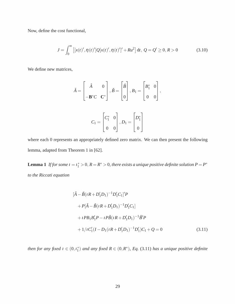
Now, define the cost functional,
J =∫ ∞
0
[[x(t)′,η(t)′]Q[x(t)′,η(t)′]′+Ru2]dt, Q= Q′ ≥ 0, R> 0 (3.10)
We define new matrices,
A=
A 0
−B∗C C∗
, B=
B
0
, B1 =
B∗1 0
0 0
,
C1 =
C∗1 0
0 0
, D1 =
D∗1
0
where each 0 represents an appropriately defined zero matrix. We can then present the following
lemma, adapted from Theorem 1 in [62].
Lemma 1 If for someι = ι∗1 > 0, R=R∗> 0, there exists a unique positive definite solution P=P∗
to the Riccati equation
[A− B(ιR+D′1D1)
−1D′1C1]
′P
+P[A− B(ιR+D′1D1)
−1D′1C1]
+ ιPB1B′1P− ιPB(ιR+D′
1D1)−1B′P
+1/ιC′1(I −D1(ιR+D′
1D1)−1D′
1)C1+Q= 0 (3.11)
then for any fixedι ∈ (0, ι∗1) and any fixed R∈ (0,R∗), Eq. (3.11)has a unique positive definite
29

stabilizing solution P, and the control law
u(t) =−(ιR+D′1D1)
−1(ιB′1P+D′
1C1)[x′(t),η ′(t)]′ ,−[K1,K2]
x(t)
η(t)
(3.12)
guarantees exponential stability of the closed-loop system (3.5) when yr(t) = w(t) = 0, and the
matrices A and B are given by(3.8)and (3.9) respectively.
3.3 Asymptotically Stable Periodic Solutions in Systems with
Hysteresis
We will now consider the behavior of the controller (3.3), (3.12) when the inputu(t) is the output
of a hysteresis operator, as assumed in (1.1). The plant output to be controlled is now modeled as
a cascade of a modified PI operator (2.16) and the dynamic system (3.1). Furthermore, we will
assume that this plant is uncertain, with the dynamic uncertainties obeying (3.8) and (3.9), and the
hysteresis uncertainty obeying Assumption 2.
We will now introduce the hysteresis inversion (2.26) into the control structure.The input to the
inversion, denoted asud(t) in (2.25), will be defined by the right-hand side of (3.12),
ud(t) =−[K1,K2][x′(t),η ′(t)]′ (3.13)
Together with (2.25), the closed-loop system (3.5) can now be written as
x(t)
η(t)
=
A−BK1 −BK2
−B∗C C∗
x(t)
η(t)
+
θ ′dDz(θ ′
hW(t))−θ ′dDz(θ ′
hW(t))
B∗yr(t)
(3.14)
30

Figure 3.1: Closed-loop system with hysteresis, as defined in(3.13), (3.14), and (2.27).
whereW(t) is defined by (2.27). A block diagram of this closed-loop system is illustrated in Fig.
3.1.
The addition of the hysteresis operator into the closed-loop system creates a series of problems
in the implementation of the servocompensator controller.First, does the system remain stable with
the state feedback (3.12)? In addition, are the trajectories of the closed-loop system periodic for
periodic reference trajectories? Such periodicity would allow us to argue that the servocompensator
can attenuate the effect of hysteresis on the closed-loop system.
If W(t) was a bounded exogenous disturbance generated by (3.2), theanswer to both questions
is clearly yes. It turns out that, if the effect of hysteresisis sufficiently small, we can also prove
both of these properties closed-loop system with hysteresis. Based on the framework presented in
Theorem 2.1 of [63], we can prove, under suitable conditionson the hysteresis operator, the exis-
tence of a unique, asymptotically stable, periodic solution. The most restrictive of these conditions
is the existence of a contraction property for the compositehysteresis operatorWd. We will see
that this condition can be met for aT-periodic reference trajectoryyr(t) if ud(t) andv(t) satisfy
the following assumption.
Assumption 5 osc[0,T][θddz(udT)] > 2rp and osc[T,2T][vT ] > 2rp where, for any continuous func-
31

tion z,
osc[t1, t2][z] = supt1≤τ≤σ≤t2
|z(τ)−z(σ)|
and rp andrp are the largest play radii forΓhd andΓ−1hd respectively.
Before proving the existence of an asymptotically stable, periodic solution, we must first show
the well-posedness of the closed-loop system. LetW1,1t be the Banach space of absolutely contin-
uous functionsu : [0, t]→ ℜ. We also equip this space with the norm
‖u‖W
1,1t
= |u(0)|+∫ t
0|u(s)|ds (3.15)
Note that, forf1, f2 ∈W1,1t the play operatorPri obeys the condition
|Pri [ f1;a](s)−Pri [ f2;a](s)| ≤ ‖ f1(s)− f2(s)‖∞
This property along with (2.29) allows us to prove that the composite hysteresis operatorWd is
Lipschitz continuous, i.e.
‖Wd[ f1;W(0)](s)−Wd[ f2;W(0)](t)‖ ≤ L‖ f1− f2‖∞
It is then clear that the right-hand side of (3.14) is Lipschitz continuous, and so the existence and
uniqueness of the solution can be established through the typical contraction mapping argument
[64]. Similar continuity properties can be proved for the dependence of the system on initial
condition; therefore the system (2.27), (3.13), and (3.14)is well posed. We are now prepared to
prove the following theorem.
Theorem 1 Consider the closed-loop system(2.27), (3.13), and(3.14). Let Assumptions 2-5 hold,
32

and let the reference trajectory yr(t) be periodic with period T . Then, there exists anε such that
if εd < ε, whereεd = max(‖θh‖,‖θd‖), the solutions of the closed-loop system(2.27),(3.13), and
(3.14), under any initial condition(x(0),η(0),W(0)), will converge asymptotically to a unique
periodic solution.
Proof. Consider an inputf (t) with osc[0,T][ f (t)]> 2r. Let Pr be a play operator with radiusr.
From (2.1) it can be seen that this play operator obeys the contraction property
|Pri [ f ;a](t)−Pri [ f ;b](t)|= 0, ∀t > T
for any two applicable initial conditionsa andb. From (2.13),W is a composite hysteresis opera-
tor, formed by the inverse PI operatorΓ−1hd , whose largest play radius is ¯rp and the play operators
of Γhd, where the largest play radius isrp. Assumption 5 therefore implies that, fort > 2T,
|W [ud;Wa(0)](t)−W [ud;Wb(0)](t)|= 0 (3.16)
for any two applicable initial conditionsWa(0) andWb(0). We will also note that the modified PI
operator (and thereforeW ) satisfies the Volterra property
f1(s) = f2(s),0≤ s≤ t ⇒ Γhd[ f1;W(0)](t) = Γhd[ f2;W(0)](t), ∀t ≥ 0 (3.17)
and the semi-group property
Γhd[ f2;Γhd[ f1;W(0)](t1)](t2− t1)≡ Γhd[ f1;W(0)](t2), if f2(t) = f1(t − t1) (3.18)
Finally, we know from the definition of the play operators andthe modified PI operator that there
33

Figure 3.2: Equivalent block diagram for the closed-loop system (2.13),(3.13), and (3.14) in steadystate analysis.
exist constantsag andbg such that the growth condition
‖W(t)‖ ≤ ag‖ud(t)‖+bg, ∀t (3.19)
is satisfied. From our discussions in Section 3.2, we know that if εd = 0, i.e. θh = θd = 0, the
closed-loop system possesses a globally exponentially stable T-periodic solution(xT(t),ηT(t)).
Therefore, the closed-loop system fits into the class of systems considered in Theorem 2.1 of
[63], and for a sufficiently smallεd there exists an asymptotically stableT-periodic solution
(x(t),η(t),W(t)) for the closed-loop system (2.13),(3.13), and (3.14).
Remark 3 This Theorem can also be applied to a classical PI operator, by consideringθd = 0.
Having now established the existence, uniqueness, and stability of the periodic solution(x(t),η(t),W(t)),
we can now discuss the steady state performance of the controller. From theT-periodicity ofW(t),
we can equivalently write the inversion error (2.26) as the Fourier series
α(t) = θ ′dDz(θ ′
hW(t))− θ ′dDz(θ ′
hW(t)) = c0+∞
∑k=1
ck sin(2πkt
T+φk) (3.20)
for some constantsφ1,φ2, · · · andc0,c1, · · · ≥ 0. We have now shown that the effect of hysteresis
at steady state can be reduced to an equivalent exogenous disturbanceα(t), as we illustrate in
34

Fig. 3.2. We therefore separate the disturbanceα(t) into two components. Let us assume that the
matrixC∗ in our servocompensator (3.3) has been chosen such that its eigenvalues are located at
± jkω, k∈ ρ, whereρ is a finite element vector of whole numbers, and then define
αc(t) = c0+ ∑k∈ρ
ck sin(2πkt
T+φk) (3.21)
αd(t) = ∑k/∈ρ
ck sin(2πkt
T+φk)
From the properties of the servocompensator, we know that any effect of the disturbanceαc will
be eliminated from the system at steady state. Therefore thetracking error under the proposed
control scheme will be of the order ofαd, which can be made arbitrarily small by accommodating
a sufficient number of harmonics in the servocompensator design.
3.3.1 Output Feedback Control of Systems with Servocompensators
It should be noted that there are many other ways of designingthe desired stabilizing controlud(t),
as opposed to the riccati equation approach presented in (3.12). A variety of techniques including
LQG control,H∞ control, or observer theory can be used to stabilize the closed-loop system. In the
interest of our experimental implementation, we will now discuss the implementation of an output
feedback controller in our closed-loop system. We will use aluemberger observer,
ˆx(t) = Ax(t)+Bud(t)+L(y(t)−Cx(t)) (3.22)
which transforms (3.13) into
ud(t) =−[K1,K2]
x(t)
η(t)
(3.23)
35

The gain vectorL is chosen so thatA−LC is a hurwitz matrix. The design of luenberger observers
requires the plant matricesA andB to be known; therefore in the case of output feedback we require
the uncertainty∆∗ to be identically zero to show stability. Under this assumption, we can integrate
the observer into the control loop, which results in the closed-loop system
x(t)
η(t)
˙x(t)
=
A −BK2 −BK1
−B∗C C∗ 0
LC −BK2 A−BK1−LC
x(t)
η(t)
x(t)
+
θ ′dDz(θ ′
hW(t))−θ ′dDz(θ ′
hW(t))
B∗yr(t)
0
(3.24)
where the system matrix is Hurwitz. As this system possessesan exponentially stableT-periodic
solution whenεd = 0, we can apply Theorem 2.1 of [63] and conclude stability of the closed-loop
system in an identical manner to the proof of Theorem 1.
3.4 Experimental Implementation of Proposed Controller
3.4.1 Nanopositioner Modeling
We now examine the performance of the proposed control scheme on a piezo-actuated nanopo-
sitioner, shown in Fig. 3.3. We have discussed the practicalimportance along with the need for
improved controllers for nanopositioning in Chapter 1. Thisplatform therefore provides a valuable
and practically relevant test of our controller’s performance in systems with hysteresis.
The first step in our experimental tests involves model identification for the piezo-actuated
nanopositioner. The hysteretic behavior was experimentally characterized using a quasi-static in-
put, which sweeps the positioner output over its operational range. As seen in Fig. 3.4, the hystere-
36

Nanopositioner
Power amplifier
Figure 3.3: Nanopositioning stage used in experimentation, Nano-OP65 nanopositioningstage coupledwith a Nano-Drive controller from Mad City Labs Inc, with a primary resonance of 3 kHz. Position feedbackis provided by a built-in capacitive sensor.
sis loop is not odd-symmetric; therefore we use a modified PI operator (2.24) with with 9 deadzone
elements and 8 play elements to model the asymmetric hysteresis. In addition, a bias scheme was
used to center the hysteresis loop about the origin; this wasaccomplished by subtracting 25.9µm
from the plant output and 4V from the plant input in the modeling procedure. The radiir and
thresholdsz were chosen based on the input and output range of the plant,
r =[0,0.33,0.66,1.00,1.33,1.66,2.00,2.33]′
z=[−2.68,−1.97,−1.22,−0.42,0,0.32,1.02,1.76,2.57]′
We then identify the model weightsθh andθd using quadratic optimization routine outlined in [32]:
θh =[0.719,0.183,0.035,0.055,0.034,0.033,0.023,0.061]′
θd =[1.062,0.473,0.641,0.311,8.426,−0.636,−0.501,−0.614,−0.415]′
The model weightsθh andθd are then used to calculate the inverse operator,Γ−1hd [ud,W(0)](t).
Since the modelΓhd is generated by biasing the input and output, we are requiredto subtract 25.9
37

1 2 3 4 5 6 7 80
10
20
30
40
50
60
70
Input (V)
Out
put (
µm)
Figure 3.4: Measured hysteresis loops for the nanopositioner.
from the inversion input and add 4 to the inversion output to maintain the inversion structure. A
comparison between the model and plant output is shown in Fig. 3.6. The discrepancy between
the model prediction and the actual measurement was around 1µm over a travel range of 45µm.
We then model the plant dynamics, using frequency response identification techniques with
small-amplitude sinusoidal inputs to reduce the impact of hysteresis on the measurements. We
found that a fourth-order plant model matched the measured frequency response reasonably well,
up to 3.5 kHz. We also set the DC gain of the dynamics to zero, since the DC gain is accounted for
in the hysteresis operator. This model has the transfer function
G(s) =8.8×10¹⁶
s4+1.6×10⁴s3+6.6×10⁸s2+5.3×10¹²s+8.8×10¹⁶ (3.25)
Note that the combination of high resonant frequency and order has resulted in very large numbers
in (3.25). In order to improve computation accuracy, we useda balanced state-space realization
38

0 20 40 60 80 100
0
10
20
30
40
50
Time (s)
Out
put (
µm)
Experiment data Model Prediction
Figure 3.5: Plant output used in the identification of the modified PI operator, and resulting modeloutput.
10 15 20 25 300
20
40
60
Time (s)
Out
put (
µ m
)
ActualModeled
10 15 20 25 30−1
0
1
2
Time (s)
Err
or (
µ m
)
Figure 3.6: Model prediction and experimental data for a decreasing sinusoid used to optimize thehysteresis model.
39

[65] in our control design:
x(t) =1.0×10⁴
−0.014 1.700 0.095 −0.050
−1.700 −0.241 −0.672 0.170
0.095 0.672 −1.066 1.617
0.050 0.170 −1.617 −0.305
x(t)+
27.8
111.3
−116.5
−44.1
u(t)
y(t) =
[27.8 −111.3 −116.5 44.1
]x(t) (3.26)
These matrices then define the nominal plant matrices(A, B,C,0), as defined in 3.8 and 3.9.
We next designed our robust stabilizing control (3.12). We then tested how the model parameters
varied by loading weight onto the nanopositioning stage. Wefound that with a maximum load, the
parameters of (3.25) varied by around±5%. Therefore, we designed our controller to be robust
to changes of±10% in the parameters of (3.25). We then translated this constraint into balanced
coordinates via the same coordinate transformation used togenerate (3.26). The resulting matrices
become theB2,C1, andD1 matrices used in (3.11). Together with the balanced coordinate system
matrices from (3.26), we can then calculate the stabilizingcontrol (3.12).
Finally, we implement a Luenberger observer to estimate thestates, as explored in Section
3.3.1. Designed and implemented in the standard manner withthe nominal state space model of
the plant, the output feedback controller is given as
ˆx(t) =Ax(t)+ Bud(t)+L(y(t)−Cx(t)) (3.27)
ud(t) =− [K1,K2]
x(t)
η(t)
(3.28)
whereL is chosen so thatA−LC is Hurwitz. In our work,L is chosen using an LQR method, and
40

equals[0.3,−3.5,−1.7,−0.23].
3.4.2 Experimental Results
We now present the results of our controller implementation. Control and measurement were
facilitated by a dSPACE platform. For comparison, we implemented an iterative learning con-
trol (ILC) algorithm [38], and a custom-designed proportional-integral controller with hystere-
sis inversion (PI+I). When discussing the proposed controller, we will distinguish between a
single-harmonic servocompensator (SHSC), and a multi-harmonic servocompensator (MHSC).
The SHSC is strictly second order, and compensates for the primary harmonic of the reference
only. The order of the MHSC will vary between experiments.
Our first set of experiments considers sinusoidal waveformsfor the reference trajectory,
yr(t) = (20sin(2πωt)+30)µm
with frequencies of 5, 25, 50, 100 and 200 Hz. Two metrics are used to quantify the tracking error.
The mean tracking error (MTE) is computed by taking the average of |e(t)| at steadty state, and
the peak tracking error (PTE) is the average of the maximum tracking error in each period of the
reference. Both metrics are computed at steady state.
Table 3.1: Tracking error results for various controllers.All results are presented as a percentageof the reference amplitude (20µm).
Reference MHSC (%) SHSC (%) ILC (%) PI+I (%)MTE PTE MTE PTE MTE PTE MTE PTE
Sine, 5 Hz 0.271 0.899 0.649 1.72 0.135 0.250 1.06 1.93Sine, 25 Hz 0.268 0.881 0.707 1.85 0.163 0.565 5.40 8.96Sine, 50 Hz 0.284 1.01 0.770 1.93 0.262 0.711 10.86 17.63
Sine, 100 Hz 0.352 1.03 0.815 2.38 0.528 1.42 21.21 33.65Sine, 200 Hz 0.519 1.57 0.863 2.50 1.31 3.20 37.61 59.6
41

Table 3.1 contains the results for each reference and controller, where the MHSC contains the
first, second, and third harmonics of the reference. The PI+Icontroller performs very poorly at
high frequencies, a problem that has been well documented [2, 39]. The ILC algorithm performs
very well in general, but cannot match the MHSC at 200 Hz, as shown in Fig. 3.7. A detailed
comparison between the ILC and MHSC methods is shown in Fig. 3.8. At low frequencies, the
ILC algorithm performs better than the MHSC. At 50 Hz, the errors are very close, with ILC still
slightly ahead. However, at 100 Hz and 200 Hz, the MHSC is significantly better, with only 40%
the mean tracking error of ILC at 200 Hz.
19.99 19.992 19.994 19.996 19.998 20
10
20
30
40
50
Time (s)
Out
put (
µm)
SHSCILCP+IMHSC
19.99 19.992 19.994 19.996 19.998 20−2
−1
0
1
2
Time (s)
Err
or (
µm)
Figure 3.7: Experimental results at 200 Hz for the proposed methods (SHSC and MHSC), ILC andPI+I.
We can also compare the performance of the multi-harmonic servocompensator (MHSC) with
that of the single-harmonic servocompensator (SHSC). From our theoretical results, we would
expect the MHSC to perform significantly and consistently better than the SHSC; this is confirmed
in Table 3.1, as the MHSC outperforms the SHSC by significant margins at each frequency for
42

5 25 50 100 2000
0.5
1
1.5
2
2.5
3
Frequency (Hz)
Err
or (
%)
MHSC MeanMHSC PeakILC MeanILC Peak
Figure 3.8: Comparison between multi-harmonic servocompensator (MHSC) and Iterative Learn-ing Control (ILC).
both error metrics. However, the performance gap narrows asthe reference frequency increases.
At 5 Hz, the MHSC has around 40% of the tracking error of the SHSC, whereas at 200 Hz the
MHSC has 60%. This can be attributed to the resonant peak of the vibrational dynamics of the
system. In particular, with increasing frequencies, the harmonics higher than the second and third
become more significant. Fig. 3.9 shows the spectra under SHSC for reference signals at 5 and 200
Hz. In both cases, the second and third harmonics of the reference signal are the most significant
in the error signal. However, the other harmonics of the system are significantly larger at 200 Hz
in comparison to the dominant second and third harmonics than they are at 5 Hz. It is therefore
reasonable to expect that canceling the second and third harmonics in the 200 Hz case would result
in reduced benefit as compared to that in the 5 Hz case.
We also demonstrate the ability for the MHSC to track sawtooth reference signals. Sawtooth
signals are commonly used in SPM applications, and represent a challenge for our proposed con-
43

0 50 100 150 2000
0.05
0.1
Frequency (Hz)
Am
plitu
de (
µm)
5 Hz
0 1000 2000 3000 4000 5000 6000 70000
0.05
0.1
Frequency (Hz)
Am
plitu
de (
µm)
200 Hz
Figure 3.9: Frequency spectra of the tracking error signal for references at 5 Hz and 200 Hz. AnSHSC was used in each case. Graphs are aligned so that the peaks on each graph correspond to thesame harmonic of the reference. Note the prominence of the harmonics near 3000 Hz in the 200Hz plot.
44

troller since they do not have a finite-dimensional internalmodel. However, by using the first few
harmonics of the signal, we can arrive at a reasonable approximation. Fig. 3.10 and Table 3.2
show tracking error results for the three control methods used, where the MHSC incorporated the
first 6 odd harmonics of the reference. The ILC controller is well suited to tracking signals like a
sawtooth, and this is shown in the tracking results. While thePI+I controller has reasonable per-
formance at 5 Hz, its performance falls off dramatically at 50 Hz. The MHSC does a significantly
better job than the P+I controller at tracking this signal, with an average error that was only 20%
of what was achieved by the latter controller at 50 Hz. While the tracking error under the MHSC
is almost five times of that under ILC at 5 Hz, it becomes comparable to that of ILC with smaller
maximum error at 50 Hz, indicating that the MHSC can facilitate tracking of such sawtooth signals.
Table 3.2: Tracking errors results for a Sawtooth signals. All results are presented as a percentageof the reference amplitude (20µm).
5 Hz (%) 50 Hz (%)MTE PTE MTE PTE
MHSC 0.562 4.15 1.08 4.26ILC 0.114 0.775 0.808 5.70P+I 1.08 1.30 10.3 12.1
We also test the performance of the proposed controller under more complex inputs. Fig. 3.11
shows the experimental results for the MHSC and ILC with a reference signal of
yr(t) = 5sin(2π5t −π/2)+5sin(2π15t +π/2)+10sin(2π25t −π/2)
Such an input excites more complex memory states for hysteresis than a sinusoidal or sawtooth
input, and is a useful test of the proposed controller’s ability to compensate for hysteresis. For
this experiment, the MHSC is designed to compensate for the reference signal alone, yielding a
6th order servocompensator. The resulting mean tracking errors are 0.52% for the MHSC and
45

19.96 19.965 19.97 19.975 19.98 19.985 19.99 19.995 20
10
20
30
40
50
Time (s)
Out
put (
µm)
MHSCILCP+I
19.96 19.965 19.97 19.975 19.98 19.985 19.99 19.995 20−2
−1
0
1
2
Time (s)
Err
or (
µm)
Figure 3.10: Experimental results at 50 Hz for sawtooth reference signal. Two periods are shown.
0.66% for ILC. Even though the reference is fairly slow, the advantage that ILC possesses at low
frequencies for the sinusoidal references has been reversed in this test by the MHSC. This proves
the effectiveness of the proposed controller at compensating for hysteresis in general systems.
Finally, we investigated the robustness of the system’s performance to loading conditions. To
prevent damage to the nanopositioner, we limited our experiments to 40% (200 g) of the maximum
load recommended by the manufacturer. ILC and a MHSC (accommodating first three harmonics)
were used for this study. Table 3.3 shows the results for tracking a 50 Hz signal for the loaded
operation, as well as the percent-change from the nominal results presented in Table 3.1. The
performance of the MHSC is nearly unchanged from the unloaded case, a point also readily visible
in Fig. 3.12. The ILC controller, however, has suffered a notable drop in performance, with double-
digit percentage drops in accuracy in the loaded case. However, due to ILC’s better performance in
the unloaded case, both methods are very close in the raw performance. This result indicates that
46

24.8 24.85 24.9 24.95 2510
20
30
40
50
Time (s)
Pos
ition
(µm
)
MHSCILC
24.8 24.85 24.9 24.95 25−0.5
0
0.5
Time (s)
Tra
ckin
g E
rror
(µm
)
Figure 3.11: Experimental results for a reference trajectory of yr = 5sin(2π5t − π/2) +5sin(2π15t +π/2)+10sin(2π25t −π/2)
47

19.98 19.985 19.99 19.995 20−0.2
−0.15
−0.1
−0.05
0
0.05
0.1
0.15
0.2
0.25
0.3
Time (s)
Err
or (
µm)
No Load200g Load
Figure 3.12: Tracking errors for a 50 Hz reference signal, for loaded and unloaded nanopositioner.An MHSC was used in both cases. Note the similarity in the timetrajectory of the tracking error.
the MHSC’s performance is significantly less tied to modelingaccuracy than ILC’s, since the net
effect of a load is to deviate the plant from its nominal dynamics, which proves the performance
robustness properties discussed in Section 3.3.
Table 3.3: Loading performance for MHSC and ILC. First two columns are presented as a percent-age of the reference amplitude (20µm), second two columns are percent change from the unloadedcase.
MTE PTE ∆ MTE ∆ PTEMHSC 0.288 0.940 1.41 -6
ILC 0.308 0.775 18.5 10.7
48

Chapter 4
Harmonic Analysis of Hysteresis Operators
with Application to Control Design for
Multi-Harmonic Servocompensators
4.1 Introduction
We now provide a design tool for the MHSC proposed in this dissertation. Consider the expression
(3.21), which describes the effect of hysteresis on the closed-loop system at steady state, and let
Gαe denote the transfer function fromα(t) to e(t) of the nominal closed-loop system (2.13), (3.13),
and (3.14) whereεd = max(‖θh‖,‖θd‖) = 0. If αd is known, the steady state function fore(t) can
be derived from the expressione(t) = Gαe(s)[αd(t)]. However, the trajectory ofαd is dependent
on the hysteresis operator; specifically, the amplitudesck and phasesφk are unknown functions of
the system parameters and hysteresis operator. Theoretically, it is possible that these coefficients
are prohibitively large; however, we can see from our experimental results thatαd is reasonably
small.
Recall from Chapter 3 that the order of the servocompensator can be used directly as a design
aid to improve tracking performance. As a control engineer,it is desirable to obtain the minimum
order and complexity for the controller to accomplish a given objective. Existing design techniques
49

for the MHSC consist of repeated iterations of different controller orders until the desired perfor-
mance is met, which is bothad hocand time consuming. Therefore, it is of interest to evaluatethe
harmonic components of a hysteresis operator in terms of thehysteresis parameters.
We now present our results on such an algorithm, which evaluates the Fourier coefficients
[66] of the output produced by a hysteresis operator in an open-loop system. This algorithm is
applicable to both PI and PKP operators, and has two primary components. First, we form the
output of the hysterons using a series of pulse signals. The pulse signals are defined through a set of
time instants at which the hysteresis behavior switches, and they are determined by a combination
of the input signal and operator parameters. Second, we use this formulation to compute the Fourier
series of the output. For the example of a play operator subject to a sinusoidal or sawtooth signal,
we provide explicit expressions for the coefficients, whichare functions of the input amplitude and
the hysteron parameters. We will also show that the resulting expressions provide some valuable
control design tools for closed-loop systems such as that inChapter 3.
4.2 Open-Loop Computation of Hysteresis Operator Outputs
Recall that any periodic signalσ(t) with periodT , 2π/ω can be written as an infinite summation
in the form
σ(t) = a0/2+∞
∑n=1
ancos(ωnt)+bnsin(ωnt) (4.1)
where the coefficientsan andbn are defined by the integrals
an =2T
∫ T
0σ(t)cos(ωnt)dt (4.2)
bn =2T
∫ T
0σ(t)sin(ωnt)dt (4.3)
50

For a Preisach-like operator, the Fourier series coefficients of its output can be constructed from
those of its constituent hysterons. To see this, consider the example of a PI operator. Recall that
the output of any play operator is described by its state, which we have defined asWr i [v;W(0)](t).
Say that we have calculatedWr i [v;W(0)](t) in the Fourier series form
Wr i [v;W(0)](t) = ai0/2+∞
∑n=1
ain cos(ωnt)+bin sin(ωnt) (4.4)
Then the Fourier series coefficients ofu(t) = Γ[v](t) can be calculated from (2.3) as
a0 =m
∑i=1
θiai0, an =m
∑i=1
θiain, bn =m
∑i=1
θibin (4.5)
A similar expression can be quickly derived for the PKP operator as well. Therefore, we will focus
our attention on computing the Fourier series for the outputof an individual hysteron. We will
begin with the play operator, defined in (2.1).
4.2.1 Harmonic Analysis of a Play Operator
In order to compute the Fourier series of a play operator’s output, we first need an analytical
expression for which a Fourier transform can be easily evaluated. We describe the output as a
function of the input as well as a series of pulse wave signalsP1, P2, andP3, determined by a set of
time instantsTi = [ti1, ti2, . . . ] andTo = [to1, to2, . . . ]. For a general input, we define the output of a
play operatoru(t) as
u(t) = (v(t)+P1(t))P2(t)+P3(t) (4.6)
51

where
P1(t) =− r(sgn(v(t))) (4.7)
P2(t) =
0, t ∈ [ti j , to j),∀ j = 1,2, . . .
1, t ∈ [to j , ti( j+1)),∀ j = 1,2, . . .
(4.8)
P3(t) =
v(ti j)− r(sgn(v(t−i j ))), t ∈ [ti j , to j)
0, otherwise(o.w.)
(4.9)
andv(t) is the input to the operator. We will assume that the time variable has been shifted so
thatu(0) lies in the linear region of the play operator. The time instantsTi andTo are determined
systematically based on the reference signal and the radiusof the play operator. In particular,ti j is
the first time satisfying the conditions
v(ti j) = 0, ti j > to( j−1), sgn(v(t−i j )) 6= sgn(v(t+i j ))
This represents the time when the output of the play operatortransitions from a linear region into
the flat “play” region. In contrast,to j is the time period when the output moves out of the “play”
region, and is the first time satisfying either
|v(ti j)−v(to j)| ≥ 2r, to j ≥ ti j ,
or
sgn(v(t+i j ))v(to j)< sgn(v(t+i j ))v(ti j), to j ≥ ti j
52

Figure 4.1: A sample curve showing how the time instantsTi and To are calculated for a playoperator. The variabler is the radius of the play operator, and it is assumed that the input at timezero is 2r.
Two cases exist for the definition ofto j since there are two ways to exit the play region of the play
operator. The first case deals with the output leaving the play region by entering the opposite linear
portion from the one it entered. Naturally then, the second case deals with the output leaving the
play region by entering the same linear portion as the one it entered from.
Fig. 4.1 shows an example of how the time instantsTi andTo are calculated for one portion of
a periodic signal. The inflection point markedti1 defines the first element ofTi. to1 is defined by
the graph returning to the level of 5r, since the curve did not fall 2r from its value atti1. ti2 is the
next inflection point afterto1 and the third such point plotted on the graph. Finally,to2 is defined
by the point where the graph has fallen 2r from its value atti2.
As a further illustration, Fig. 4.2 demonstrates how the play operators output is reconstructed
from the input and pulse signals. The reference signal is assumed to be a sinusoid with amplitude
of two, and the play operator possesses a radius of 0.3. The vertical dashed lines indicate the time
instants for this particular reference and play operator.P1(t) controls the offset or lag generated
53

4 6 8 10 12 14
−1.7
0
1.7−1.7
0
1.70
1
−.30.3
−2
0
2
ti1
to1
ti2
to2
u(t)
P3(t)
P2(t)
P1(t)
v(t)
Figure 4.2: Reconstruction of the outputu(t) of a play operator. The play radiusr = 0.3, and thetime axis is shared by each signal.
54

by the play operator in the linear regions.P2(t) “switches” the output between the play and linear
regions of the operator, whileP3(t) “holds” the output when the play operator is in the “play”
region.
Having now expressed the output of the play operator in the form (4.6), we can compute the
Fourier series of the outputu(t). Using (4.6) along with (4.7)-(4.9), we can break up the integrals
in (4.2) and (4.3) as
an =2T
[∫ to1
ti1(P3(t))cos(ωnt)dt
+∫ ti2
to1
(v(t)+P1(t))cos(ωnt)dt
+∫ to2
ti2(P3(t))cos(ωnt)dt + · · ·
](4.10)
bn =2T
[∫ to1
ti1(P3(t))sin(ωnt)dt
+∫ ti2
to1
(v(t)+P1(t))sin(ωnt)dt
+∫ to2
ti2(P3(t))sin(ωnt)dt + · · ·
](4.11)
The complexity of calculatingan andbn depends greatly on the form ofv(t) as well as how complex
the definitions for the time indicesTi andTo are in order to describe the signal. However, we can
arrive at simple and analytical expressions for some commontypes of input signals.
4.2.2 Example Calculations for a Sinusoidal Input
We will now present some sample calculations of the Fourier series coefficients for the play oper-
ator. For a sinusoidal input, we can derive the final expressions foran andbn of the harmonics as
55

explicit functions of the amplitude and the play radius. Consider a sinusoidal input
v(t) = Asin(ωt) (4.12)
We assumeA ≥ r, which ensures a contraction property like (3.16); thus thesteady-state play
output is independent of the initial condition. Sinusoidalsignals are easy to deal with utilizing the
proposed algorithm because they possess only two inflectionpoints per period, which gives the
pulse signalsP1(t), P2(t), andP3(t) very simple forms. The first step in the computation of (4.10)
is to obtain the time instantsTi andTo,
ti j =T4+
( j −1)T2
(4.13)
to j =T2− sin−1(1−2r/A)
ω+
( j −1)T2
(4.14)
We can then write (4.10) as
an =2T
[∫ to1
ti1(A− r)cos(ωnt)dt
+A∫ ti2
to1
(sin(ωt)+ r)cos(ωnt)dt
+∫ to2
ti2−(A− r)cos(ωnt)dt
+ A∫ T+ti1
to2
(sin(ωt)− r)cos(ωnt)dt
](4.15)
56

This results in two types of integrals to evaluate, whose solutions forn> 1 are given by
∫cos(ωnt)dt =
sin(ωnt)ωn
∫sinωt cos(ωnt)dt =
cos((n−1)ωt)2ω(n−1)
− cos((n+1)ωt)2ω(n+1)
(4.16)
Using these integrations combined with (4.13)-(4.15), we can arrive at a closed-form expression for
each individualan. The expressions forbn can be derived in a similar way. Furthermore, because
of the form for the limits of integration, we can simplify this expression forn> 1. In particular,
because of the appearance of sin−1 along with half and quarter periods, simplified expressionscan
be found devoid of any trigonometric functions. For example, whenn= 3,
a3 =−4r(8r3−16Ar2+9A2r −A3)
3A3π(4.17)
and
b3 =−16r(2r2−3Ar+a2)√
r(A− r)
3A3π(4.18)
Furthermore, we can computec3 =√
a23+b2
3, which simplifies to
c3 =4r(A− r)
3Aπ(4.19)
while for n= 5,
c5 =4r(A− r)
√32r2−32Ar+9A2
15A2π(4.20)
Fig. 4.3 and 4.4 show the calculated values ofcn as functions of the amplitudeA and the play
radiusr respectively. The even harmonics are always zero due to the odd symmetry of the play
operator. Fig. 4.3 shows the relative size of harmonic coefficients trending towards zero with
57

increasingA. Such a behavior is anticipated, because the hysteresis loop for a fixed play radius
appears narrower and narrower as the amplitude of the input is increased. From Fig. 4.4, we can
see that the relative amplitude of the harmonics varies greatly with the play radius. In particular,
for a play radiusr = A/2, c3 is five times as large asc5, yetc5 andc7 are almost identical in size.
But for r = A/4, c5 is over three times the value ofc7. However, from both Fig. 4.3 and 4.4, we
see that higher harmonics are always less significant that lower harmonics. Such graphs can serve
as a valuable design tool for systems such as that consideredin [67], as we will be able to estimate
the relative sizes of the harmonics within the systema priori.
0 2 4 6 8 10 120
0.02
0.04
0.06
0.08
0.1
0.12
Amplitude (A)
c n/A
3rd5th7th9th11th13th
Figure 4.3: Plot ofcn for increasing amplitudeA. The play radius is held constant atr = 0.5.
4.2.3 Example Calculations for a Raster/Sawtooth Input
We also investigate the application of the algorithm to a raster or sawtooth input signal in combi-
nation with a play operator. As we have seen, such inputs are particularly relevant in atomic force
58

0 A/4 A/2 3A/4 A0
0.02
0.04
0.06
0.08
0.1
0.12
Play Radius (r)
c n/A
3rd5th7th9th11th13th
Figure 4.4: Plot ofcn for increasing play radiusr. Values ofcn andr are normalized by the inputamplitudeA.
microscope applications [23]. We can write the inputv(t) with amplitudeA and periodT as
v(t) =
4AT (t −Tn), if t ∈ [−T
4 +Tn, T4 +Tn]
−4AT (t −Tn−T/2), if t ∈ [T4 +Tn, 3T
4 +Tn]
(4.21)
for n = 1,2, · · · . Similar to sinusoidal inputs, raster signals have only twoinflection points per
period, allowing us to easily calculateTi andTo as
ti j =T4+
( j −1)T2
to j =T(2r +A)
4A+
( j −1)T2
59
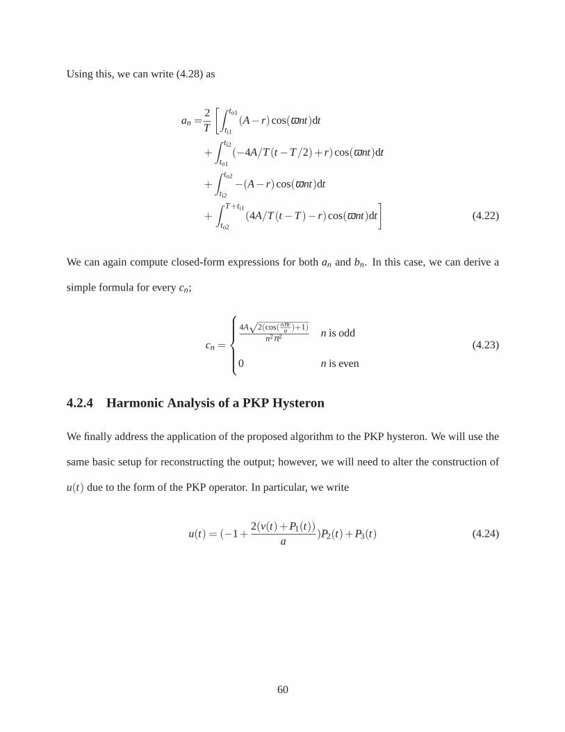
Using this, we can write (4.28) as
an =2T
[∫ to1
ti1(A− r)cos(ωnt)dt
+∫ ti2
to1
(−4A/T(t −T/2)+ r)cos(ωnt)dt
+∫ to2
ti2−(A− r)cos(ωnt)dt
+∫ T+ti1
to2
(4A/T(t −T)− r)cos(ωnt)dt
](4.22)
We can again compute closed-form expressions for bothan andbn. In this case, we can derive a
simple formula for everycn;
cn =
4A√
2(cos( nπra )+1)
n2π2 n is odd
0 n is even
(4.23)
4.2.4 Harmonic Analysis of a PKP Hysteron
We finally address the application of the proposed algorithmto the PKP hysteron. We will use the
same basic setup for reconstructing the output; however, wewill need to alter the construction of
u(t) due to the form of the PKP operator. In particular, we write
u(t) = (−1+2(v(t)+P1(t))
a)P2(t)+P3(t) (4.24)
60

whereP1(t), P2(t), andP3(t) are defined by
P1(t) =
−α sgn(v(t))> 0
−β sgn(v(t))< 0
P1(t−) sgn(v(t)) = 0
(4.25)
P2(t) =
0, t ∈ [ti j , to j),∀ j = 1,2, . . .
1, t ∈ [to j , ti( j+1)),∀ j = 1,2, . . .
(4.26)
P3(t) =
−1+2(v(ti j )−α)
a sgn(v(t−i j ))> 0 andt ∈ [ti j , to j)
−1+2(v(ti j )−β )
a , sgn(v(t−i j ))< 0 andt ∈ [ti j , to j)
0, o.w.
(4.27)
The definitions above are slightly different from those listed in (4.7)-(4.9). The other major differ-
ence between the cases of the PKP hysteron and the play operator is in the definitions of the time
instantsTi andTo. In particular, there are some extra conditions for definingeachti andto. As with
the play operator, for the PKP hysteron,ti can be defined by an inflection point in the input signal
v(t). However, we will also useti to define times when the input saturates the PKP operator, i.e.,
ti j is the first time satisfying the condition
v(ti j) = 0, ti j > to( j−1),sgn(v(t−i j )) 6= sgn(v(t+i j )),
or
v(ti j)< β , ti j > to( j−1),
61

or
v(ti j)> α +a, ti j > to( j−1).
Since we have added conditions to the definition ofti we must also add conditions to the definitions
of to related to exiting the saturation regions. Therefore,to j is the first time satisfying the condition
|v(ti j)−v(to j)| ≥ α −β , to j ≥ ti j ,
or
sgn(v(t+i j ))v(to j)< sgn(v(t+i j ))v(ti j), to j ≥ ti j ,
or
v(to j)> α, v(ti j) = β , to j > ti j
or
v(to j)< β +a, v(ti j) = α +a, to j > ti j .
where the saturation within the PKP hysteron has added the final two conditions. The first two
conditions listed serve the same roles they did with the playoperator; namely exiting the center
“play” region from the opposite or the same side as the signalentered. Once the time indicesTi
andTo are defined, the Fourier coefficients can be calculated in thesame manner as they were in
62

Section 4.2.1, by evaluating the integrals
an =2T
[∫ to1
ti1(P3(t))cos(ωnt)dt
+∫ ti2
to1
(−1+2(v(t)+P1(t))
a)cos(ωnt)dt
+∫ to2
ti2(P3(t))cos(ωnt)dt + · · ·
](4.28)
bn =2T
[∫ to1
ti1(P3(t))sin(ωnt)dt
+∫ ti2
to1
(−1+2(v(t)+P1(t))
a)sin(ωnt)dt
+∫ to2
ti2(P3(t))sin(ωnt)dt + · · ·
](4.29)
4.3 Illustration in Controller Design
We will now explore the use of the proposed analysis in the design of controllers like those pro-
posed in Chapter 3. We consider a closed-loop system
x(t)
η(t)
=
A 0
−B∗c C∗
x(t)
η(t)
+
B(ud +θWr [ud;W(0)](t))
B∗yr(t)
ud(t) =[K1,K2]
x(t)
η(t)
yr(t) =asin(2πt) (4.30)
whereA=−B=−20π, c= 1, x∈ ℜ, andθ = 0.1. This system represents a simplified version of
the system considered in Chapter 3. The variablex refers to the state and output of our example
plant, whileη is the state vector of the servocompensastor. The vectorB∗ and matrixC∗ are chosen
63

as a controllable pair where the eigenvalues ofC∗ are predetermined harmonics of the reference
frequency 2π. As discussed in Chapter 3, an important step in the design of such a controller is the
selection of which harmonics will be compensated by the servocompensator. For this simulation,
we will consider controllers compensating the (a) the first harmonic, (b) the first and third, and
(c) the first, third and fifth harmonics, implyingη ∈ ℜ2, η ∈ ℜ4, andη ∈ ℜ6 respectively. The
control gains[K1,K2] are selected using the well known LQR technique [60], whereQ is set to an
appropriately sized identity matrix, andR= 1. The value ofa= 0.931 is chosen as the amplitude of
ud necessary for an open-loop sinusoidal input to output a signal of unit amplitude whenr = .5. We
will use two different play radii,r = A/2 andr = A/4, and investigate the differences in tracking
error for the three controllers discussed above.
For such a system, it is desirable to meet a required trackingerror target with a minimum-
order servocompensator, as increasing the order of the servocompensator increases the computa-
tion power needed to accomplish the control task. However, there are no existing guidelines for
selecting the order of the compensator, and thus the order ofthe compensator is the result of a
guess-and-check process. Now, based on Fig. 4.4, we are ableto make some educated design
decisions concerning the order of the servocompensator. When r = a/2, we would expect com-
pensating for the third harmonic to have a much greater impact than whenr = a/4. Likewise,
compensating for the fifth harmonic should be more effectivewhenr = a/4 as compared to when
r = a/2.
Fig. 4.5 confirms these expectations. When only the first harmonic is compensated, we notice
that the error is significantly higher whenr = a/2, where the mean tracking error is 4.41×10⁻³,
as compared withr = a/4, where the error is 3.26×10⁻³. A larger play radius can be interpreted
as a larger hysteresis effect, which explains this initial difference. Once the third harmonic is
compensated, the tracking error in ther = a/2 case becomes lower than ther = a/4 case, with the
64

tracking errors being 0.97×10⁻³ against 1.15×10⁻³. Finally, the situation reverses again when
the fifth harmonic is compensated, with ther = a/4 case leadingr = a/2 case, where the errors
are 0.43×10⁻³ and 0.61×10⁻³ respectively. These results give us some general guidelines on the
selection of the controller order, which can be based on which weights of the PI operator possesses
the largest amplitude.
1 530
0.5
1
1.5
2
2.5
3
3.5
4
4.5x 10
−3
Highest Harmonic Compensated
Mea
n T
rack
ing
Err
or
r = a/2r = a/4
Figure 4.5: Mean tracking errors for various controllers and play radii. Note that the controllergains and structure is unchanged by altering the play radius.
Furthermore, we can use the equations (4.19) and (4.20) to achieve an estimation for precisely
how much effect the compensation of each harmonic will have in the closed-loop system. Consider
a system (4.30) withθWr [ud;W(0)](t) replaced by a fictitious external disturbanceα(t). Let φ(s)
be the transfer function fromα(t) to the tracking errore(t) = yr −Cx, which can be calculated
from the state space form of (4.30) [60]. We can then estimatethe effect ofθWr [ud;W(0)](t) on
the tracking error through the formulaθci |φ( j2iπ)|, which gives the amplitude of theith harmonic
within e(t) for a given controller definingφ(s). This formula would be exact, if the play operator
65

was driven by an open loop sinusoid of amplitudeA, instead ofud(t). However, since the play
operator is within the loop, we can expect some error in the estimation.
It is important to note that the weightθ used in these tests is fairly small, with a value of
0.1. Recall that the expressions (4.19) and (4.20) for the Fourier coefficients used in the above
simulations were derived under the assumption that the input to the play operator was a pure
sinusoidal signal. By having a smallθ , the resulting harmonics added to the system by the play
operator are fairly small, and thusud is fairly close to an ideal pure sinusoid.
Table 4.1: Proposed algorithm’s estimations of harmonic amplitude compared with actual valuesfrom closed-loop system (4.30). Setup column gives value for play radius used and the harmonicbeing estimated.
Setup Predicted Actual % Error3rd, r = A/2 θc3|φ( j6π)|= 6.77×10⁻³ 7.00×10⁻³ −3.33rd, r = A/4 θc3|φ( j6π)|= 5.08×10⁻³ 5.01×10⁻³ 1.45th, r = A/2 θc5|φ( j10π)|= 1.68×10⁻³ 1.79×10⁻³ −6.55th, r = A/4 θc5|φ( j10π)|= 1.29×10⁻³ 1.35×10⁻³ −4.7
Table 4.1 compares the estimated harmonic values with the actual values, which are calculated
from the simulation tracking error using the Fast Fourier Transform (FFT) function of MATLAB.
Four calculations are presented, in which the harmonic being estimated is varied between the 3rd
and 5th harmonics and the play radius changed betweenr = a/2 to r = a/4. The controller is also
changed, compensating the first harmonic when the third harmonic is estimated, and compensating
the first and third when the fifth harmonic is estimated. The percent error is calculated using the
standard formula:(Predicted−Actual)/Predicted. The proposed algorithm is capable of generating
a fairly accurate estimation of the amplitude of the harmonics, with the highest error being only
6.5%. This is made more impressive by the fact that there are no other useful tools for such a
design problem.
66

Chapter 5
A Nonlinear Adaptive Servocompensator
5.1 Introduction
In Chapter 3, we demonstrated the effectiveness of servocompensators for solving tracking prob-
lems in systems with hysteresis. The design procedure for a servocompensator requires precise
knowledge of the reference frequency’s internal model to beknowna priori. However, such de-
tailed knowledge of the reference is not available in advance for many applications. In addition,
the controller parameters of the servocompensator must be changed each time the internal model
of the reference changes.
Motivated by this, we investigate the use of an adaptive servocompensator, presented in [68], to
solve the nanopositioning tracking problem when the frequency is unknown. We will make use of
hysteresis inversion to improve the compensator’s performance. A high gain stabilizing controller
provides robustness to varying loading conditions and other uncertainties in the plant dynamics.
We use parameter projection to robustify the method of [68] against a bounded input disturbance.
Then, we use similar arguments to that in Chapter 3 to show that, with a well-designed hysteresis
inversion, the remaining effect of hysteresis in the steadystate can be treated as a periodic ex-
ogenous disturbance. This, coupled with the robustness of our adaptive law, permits us to argue
that the tracking error is bounded, and its steady state value is related to the size of the exogenous
disturbance left over after inversion. We also extend the control method of [68] to accept cases of
partially known exosystems.
67

We confirm our theoretical analysis by experimentation on a commercial nanopositioning
stage. The performance of the proposed controller is compared to an iterative learning control
algorithm [38]. Average tracking error is under 1.8% at 200 Hz for an actuation range of 60% of
the stage limit. Tracking results for sawtooth signals are also presented. Since transient behavior
is important in practical applications, adaptation convergence speeds are also tested. Adaptation
parameters settle within 2 s in response to changes in the reference signal from 75 to 50 to 100
Hz. The controller is shown to be robust to loading conditions from 0−20% of maximum load.
However, we will also observe that this controller cannot make use of the principles of the MHSC,
which motivates us to consider a novel solution for this problem.
5.2 Robust Adaptive Servocompensator Design
5.2.1 System Equations and Error System
Following [68], we consider systems transformable into thenormal form,
z(t) = f0(z(t),x1(t),w(t))
x1(t) = x2(t)
· · ·
xr(t) = fr(z(t),x1(t), · · · ,xr(t),w(t))+bu(t)
y(t) = x1(t) (5.1)
wherex ∈ ℜr andz∈ ℜp. The functionsf0 and fr are unknown but smooth, withf0(0,0,0) =
0, fr(0,0, · · · ,0,0) = 0. The constantb is assumed to be positive and bounded. The vectorw∈ ℜΨ
68

is generated by a neutrally stable, linear time-invariant exosystem,
w(t) = S(σ)w(t) (5.2)
The matrixS(σ) is in general unknown, depending on the unknown parametersσ ∈ ℜΣ.
Assumption 6 The parameterσ is confined to a known compact setκσ , which subsequently con-
fines S(σ) to a known compact setκw.
The tracking error is given by
e(t) = x1(t)−q(w(t)) (5.3)
whereq(w) is the reference signal to be tracked. The objective of our control design is to minimize
the tracking errore. It should be noted that it is common for the exosystem to be partially known.
For example, many reference trajectories will contain a constant bias term. The differences be-
tween the partially known case and the fully unknown case will be pointed out at the end of our
analysis. Following [57], we make the following assumptionto ensure that the tracking problem is
well-posed.
Assumption 7 For every S∈ κw, there exists a globally defined solutionζσ (w) to the equation
∂ζσ (w)∂w
Sw= f0(ζσ (w),q(w),w) (5.4)
This assumption and the triangular structure of (5.1) ensure the existence of a unique, globally
defined solution(z,x,u) = (ζσ (w),ϑσ (w),cσ (w)) to the system (5.1), given by
69

ϑσ (w(t)) =
q(w(t))
LS(σ)wq(w(t))
· · ·
Lr−1S(σ)wq(w(t))
cσ (w(t)) =1b[Lr
S(σ)wq(w(t))− fr(ζσ (w(t)),ϑσ (w(t)),w(t))]
whereLlρg(·) represents thel th Lie derivative [64] ofg(·) with respect toρ.
Assumption 8 There exists a j∈N, j ≥Ψ and a vector of real numbers[a0(σ),a1(σ), · · · ,a j−1(σ)]
such that the identity
L jS(σ)wcσ (w(t)) =a0(σ)cσ (w(t))+a1(σ)LS(σ)wcσ (w(t))
+ · · ·+a j−1(σ)L j−1S(σ)wcσ (w(t))
holds for all(w,σ) ∈ ℜΨ×Σ.
Assumption 8 is required to ensure that the necessary control cσ (w) can be generated by our
internal model controller. Specifically, this implies thatthere exists a mapping
τσ (w(t)) =
cσ (w(t))
LS(σ)wcσ (w(t))
· · ·
L j−1S(σ)wcσ (w(t))
70

which satisfies
LS(σ)wτσ (w(t)) =Φ(σ)τσ (w(t))
cσ (w(t)) =Γτσ (w(t)) (5.5)
HereΦ(σ) ∈ ℜ j× j ,Γ ∈ ℜ1× j and(Φσ ,Γσ ) is an observable canonical form whose characteristic
equation is solved by the vector[1,−a j−1(σ), · · · ,−a1(σ),−a0(σ)]. Furthermore, the spectrum
of Φ(σ) contains all the distinct eigenvalues of the exosystem (5.2), and those of any harmonics of
the exosystem generated by the system (5.1). Because of this,we will refer to the pair(Φ(σ),Γ) as
the extended exosystem. The above functions(ζσ (w),ϑσ (w),cσ (w),τσ (w)) represent the states of
the plant, control signal, and extended exosystem on a zero error manifold. Using these functions
we will now form the error system, which will be used in our analysis and controller design. The
global change of coordinates
z(t) = z(t)−ζσ (w(t)), x(t) = x−ϑσ (w(t)) (5.6)
places (5.1) into the error system form
˙z(t) = f0(z(t), x1(t),w(t),σ)
˙x1(t) = x2(t)
· · ·
˙xr(t) = fr(z(t), x1(t), · · · , xr(t),w(t),σ)+b[u(t)−cσ (w(t))]
e(t) = x1(t) (5.7)
71

Assumption 9 The zero dynamics of the system(5.7),
˙z(t) = f0(z(t),0,w(t),σ)
are exponentially stable, with Lyapunov function V1 = z′Paz, where Pa is positive definite.
As a final preliminary, we will make another change of coordinates
θ(t) = xr(t)+krb0x1(t)+kr−1b1x2(t)+ · · ·+kbr−2xr−1(t) (5.8)
wherek> 0 is a constant design constant, and the polynomialλ r−1+br−2λ r−2+ · · ·+b1λ +b0 is
Hurwitz. θ represents a modified tracking error we will use in our control design. This allows us
to place the system in the form,
˙za(t) =Fa(za(t),w(t),σ ,k)+Gaθ(t) (5.9)
θ(t) =φ(za(t),θ(t),w(t),σ ,k)+b[u−cσ (w(t))] (5.10)
where
za(t) = [z(t), x1(t), · · · , xr−1(t)]′
Fa(za(t),w(t),σ ,k) =
f0(z(t), x1(t),w(t),σ)
x2(t)
· · ·
−kr−1b0x1(t)−kr−1b1x2(t)−·· ·−kbr−2xr−1(t)
Ga =(0, · · · ,0,1)′
72

and
φ(za(t),θ(t),w(t),σ ,k) = fr(z(t), x1(t), · · · , xr(t),w(t),σ)
+krb0x2(t)+kr−1b1x3(t)+ · · ·+kbr−2xr(t)
with xr replaced byθ −krb0x1−kr−1b1x2−·· ·−kbr−2xr−1.
5.2.2 Controller Design
Our control signalu(t) is composed of two components. First, we use a stabilizing controller,
ust =−Kθ , K > 0, which will make an invariant manifold of the system globally attractive. Then
we will use an internal model controller to ensure that on theinvariant manifold the tracking error
is zero (in the absence of disturbances). In preparation foradaptation, we design our internal model
in the canonical form [69]
ξ (t) = (F +Gψσ )ξ (t) (5.11)
whereξ ∈ ℜ j and the pair(F,G) is controllable, withF Hurwitz. ψσ ∈ ℜ1× j defines a state
feedback that sends the eigenvalues of(F +Gψσ ) to the eigenvalues of the extended exosystem
(5.5). The work of [69] ensures that the Sylvester equation,
Mσ Φ(σ)−FMσ = GΓ (5.12)
has a unique, nontrivial solutionMσ . We can now define the vectorψσ from the expression
Mσ Φ(σ)M−1σ = F +Gψσ , implying ψσ = ΓM−1
σ . The implemented internal model controller
73

is driven by the error termθ ,
ξ (t) = (F +Gψσ )ξ (t)+Nθ(t)
uim(t) = ψσ ξ (t) (5.13)
where the vectorN will be defined momentarily. The composite controlu(t) is then
u(t) = ust(t)+uim(t) =−Kθ(t)+ψσ ξ (t) (5.14)
We now can see that the extended exosystem (5.5) is immersed into the internal model con-
troller (5.11), with an immersion map defined as
τσ (w) = Mσ τσ (w) (5.15)
satisfying the relations,
∂ τσ∂w
S(σ)w= Mσ ΦM−1σ τσ (w)
cσ (w) = Γτσ (w)
= ψσ τσ (w)
The vectorN will be designed to render a kind of error coordinate,
ξ (t)→ χ(t) = ξ (t)− τσ (w(t))−1b
Gθ(t)
independent of the stabilizing gainK. As discussed in [68], the termξ − τσ represents the error
74

between the current states of the internal model controllerand desired states of the controller on
the zero error manifold. Including the term−1bθ simplifies the resulting equation forχ, which is
χ(t) = Fχ(t)+(1b
FG+N+GK)θ(t)− 1b
Gφ(za(t),θ(t),w(t),σ ,k) (5.16)
We can now simplify our analysis by rendering this equation independent ofK by settingN =
−KG. This allows us to represent the closed loop system as (see [68] for details),
χ(t) =Fχ(t)+1b[FGθ(t)−Gφ(za(t),θ(t),w(t),σ ,k)] (5.17)
˙za(t) =Fa(za(t),w(t),σ ,k)+Gaθ(t) (5.18)
θ(t) =φ(za(t),θ(t),w(t),σ ,k)+bψσ χ(t)+(ψσ G−bK)θ(t) (5.19)
5.2.3 Robust Adaptive Law
We now consider the case where the internal model of the exosystem (5.2) is unknown. An adaptive
law is proposed for the vectorψσ , which we will robustify to matched disturbances via parameter
projection and show that the tracking error will be bounded.Replacingψσ by ψσ and setting
ψ = (ψσ −ψσ ), equations (5.17) - (5.19) become
χ(t) =Fχ(t)+1/b[FGθ(t)−Gφ(za(t),θ(t),w(t),σ ,k)] (5.20)
˙za(t) =Fa(za(t),w(t),σ ,k)+Gaθ(t) (5.21)
θ(t) =φ(za(t),θ(t),w(t),σ ,k)+bψσ χ(t)+(ψσ G−bK)θ(t)
+bψξ (t) (5.22)
75

The adaptive law takes the form
˙ψ(t) =ϕ(ξ (t),θ(t)) (5.23)
where we will use a Lyapunov argument to defineϕ(ξ ,θ). The system (5.20)-(5.23) will be
referred to as our nominal system. We will now seek a Lyapunovfunction for the closed-loop
system. First, consider the case whereψσ is known, and no adaptation is needed. Next, define
P from the Lyapunov equationPF +F ′P = −I , whereI denotes an appropriately dimensioned
identity matrix. It can now be shown, assuming a high enough gain K and high enoughκ, the
derivative of the function
W(χ, za,θ) = χ ′(t)Pχ(t)+κ z′a(t)Paza(t)+12
θ 2(t) (5.24)
satisfies the expressionW ≤ −λ‖(χ, za,θ)‖2, whereλ is positive. Throughout the paper,‖·‖
denotes the Euclidean norm. This implies that(χ, za,θ) = (0,0,0) is exponentially stable.
Now, consider the closed loop system (5.20)-(5.23). We modify W to be
W(χ, za,θ , ψ) =W(χ, za,θ)+b2
ψ ′(t)γ−1ψ(t), γ > 0 (5.25)
Taking the time derivative ofW yields
W ≤−λ‖(χ, za,θ)‖+bψ(t)[θ(t)ξ (t)+ γ−1ϕ(ξ (t),θ(t), ψ(t))] (5.26)
76

We now can define the adaptive law by letting
ϕ(ξ ,θ , ψ) =−γθ(t)ξ (t) (5.27)
whereγ > 0 is the adaptation gain. This implies that the vectorψ converges to someψ∗, and that
the tracking errore(t)→ 0 ast → ∞.
Remark 4 If the vectorξ can be shown to satisfy a persistent excitation condition [43], in addition
to the error convergence, it can be shown thatψ → 0 as t→ ∞.
Now, we will allow a matched disturbanceα to be added to the system. This changes the
closed-loop system into
χ(t) =Fχ(t)+1/b[FGθ(t)−Gφ(za(t),θ(t),w(t),σ ,k)]−Gα(t) (5.28)
˙za(t) =Fa(za(t),w(t),σ ,k)+Gaθ(t) (5.29)
θ(t) =φ(za(t),θ(t),w(t),σ ,k)+bψσ χ(t)+(ψσ G−bK)θ(t)
+bψξ (t)+bα(t) (5.30)
˙ψ(t) =− γθ(t)ξ (t) (5.31)
To robustify the adaptive law, we will use parameter projection to constrain the estimateψσ to a
convex, compact set. This will allow us to deal with the extraterms resulting from the disturbance
α that will appear in (5.26). Our analysis here is adapted fromthe work in [70].
Assumption 10 The initial conditions of(5.20)-(5.23), given as(χ(0), za(0),θ(0)), belong to a
known compact setX0, Z0,Θ0
Because we have assumedS∈ κσ , there exists some setΩ such thatψσ ∈ Ω. We can then
77

constrain our estimationψσ to a convex, compact setΩδ ⊃ Ω. Let c1 = max(W(χ, za,θ)), where
(χ, za,θ) ∈ X0, Z0,Θ0, and
c2 = maxψσ∈Ω,ψσ∈Ωδ
12(ψσ −ψσ )
Tγ−1(ψσ −ψσ ) (5.32)
Let c3 > c1+c2, which we use to define the setE , (χ, za,θ) : W(χ, za,θ) < c3. We now aim
to show that trajectories starting in the setE stay in this set∀t > 0. Let d = max‖α(t)‖. The
derivative ofW can be written as
W ≤−λ‖(χ, za,θ)‖2+bθ(t)d+χ(t)d (5.33)
Finally, we define the constant
k1 , max(θ ,χ)∈E
(bcθ +χ) (5.34)
We can now show that there exists a constantν such that
W ≤−νW+k1d+c2 (5.35)
We can now see that there exists ad∗ such that for anyd < d∗ , ν(−c2+ c3)/k1, W < 0 on
W = c3 : ψσ ∈ Ωδ. Thus the setW ≤ c3 : ψσ ∈ Ωδ is positively invariant for alld < d∗.
This implies that the trajectories are trapped inside the set E∩Ωδ , which implies that all states are
bounded. Also, from (5.35) we can see that the tracking erroris on the orderO(d+1/(γ)).
Remark 5 If γ is replaced by a matrix Y , the above theory also holds, with tracking error on the
order O(d+1/|λmin(Y)|), whereλmin(·) denotes the minimum eigenvalue.
78
5.2.4 Partially Known Exosystem
We will briefly consider the case where the exosystem is partially known. To handle this, we will
split (5.13) into two subsystems, related to the known and unknown portions of the exosystem.
The subsystems form the internal model controller
ξ0(t)
ξ1(t)
=
F0+G0ψ0 0
0 F1+G1ψ1
ξ0(t)
ξ1(t)
+
N0
N1
θ(t) (5.36)
uim(t) = ψ0ξ0(t)+ψ1ξ1(t) (5.37)
The eigenvalues ofF0+G0ψ0 consist of the known portion of the exosystem (5.2). The existence
of (ψ0,ψ1) can be shown by partitioning the matrixΨ(σ) into known and unknown portions, and
then applying the results of [69] to each portion. To simplify our notation, we define
F∗ ,
F0 0
0 F1
, G∗ ,
G0 0
0 G1
, N∗ ,
N0 0
0 N1
We now determine the vectorsN0 andN1 using equation (5.16), which becomes
χ0(t)
χ1(t)
= F∗χ(t)+(
1b
F∗G∗+N∗+G∗K)θ(t)− 1b
G∗φ(za(t),θ(t),w(t),σ ,k) (5.38)
In order to make the above equation independent ofK, we can setN0 = G0θ , N1 = G1θ . We then
design the adaptive law in the same way withψ , (ψ0,ψ1), and use the same Lyapunov functions
to show stability and parameter convergence. However, we assume that the value ofψ0 is known
in advance. Thus, (5.26) will be independent ofψ0 andχ0, and the adaptation law will only need
to effectψ1. For the remainder of our analysis, we will assume that the exosystem is completely
79

unknown.
5.3 Analysis of Closed-Loop System including Hysteresis
Having established robustness to disturbances outside those generated by the exosystem (5.2), we
will now consider the scenario where the input to the system (5.1) is the output of a hysteresis
operator. We now include the hysteresis operator (2.3) intoour description of the closed-loop
system. After using (2.3) and (2.12) together with (5.20) to(5.23) and (5.27), the complete closed-
loop system becomes
χ(t) =Fχ(t)+1/bc[FGθ(t)−Gφ(za(t),θ(t),w(t),σ ,k)]
−Gθh′W(t) (5.39)
˙za(t) =Fa(za(t),w(t),σ ,k)+Gaθ(t) (5.40)
θ(t) =φ(za(t),θ(t),w(t),σ ,k)+bψσ χ(t)+(ψσ G−bcK)θ(t)
+bcψ(t)ζ (t)+bθh′W(t) (5.41)
˙ψ(t) =−Γθ(t)ζ (t) (5.42)
W(t) =W [ud;W(0)](t), P Γ−1[ud;W(0)](t) (5.43)
Note that the above system without hysteresis is identical to the system discussed in [68]. Since
that system was shown to admit an asymptotically stable periodic solution, the above system fits
into the class of systems discussed in [63]. We can now use this work to show that there is an
asymptoticly stable periodic solution to the system (5.39)- (5.43), and that this solution is close
to the original solution assuming that the inversion errorθh′W is small. This argument follows
identically to that presented in Chapter 3, and allows us to prove the existence of an asymptotically
80

stable periodic solution.
5.4 Expermiental Results
We will now test the performance of our method via experimentation on our commercial nanopo-
sitioning stage shown in Fig. 3.3. Due to the increased complexity of this controller, we were
required to reduce the order of the system model considered to a second order linear system,
placed in the normal form,
x(t) =
0 1
−1.795×10⁸ −5696.88
x(t)+
0
1.063×10⁹
u(t)
y(t) =[1,0]x(t)
Even doing this, the sampling rate of the system was reduced to 10 kHz, as opposed to the
20 kHz rate used in Chapter 3. Since the positioner can be faithfully modeled without zero dynam-
ics, the error system state ˜x is defined in the usual way as ˜x1 = x2− yr(t), x2 = x2− yr(t), where
yr(t) is the reference trajectory. The modified error term (5.8) ischosen asθ , x1+ x2. This makes
za = x1 andφ(za,θ ,w, p,k) =−1.795×108x1−5696.88(θ − x1)+θ − x1. Since all reference tra-
jectories included a bias term, an integral type controllerwas included into the design scheme in
accordance with the results of Section 5.3. The controller’s design parameters were chosen as
F0 =−200, G0 = 200, ψ0 = 1
81

F1 =
−500 500
0 −500
, G1 =
0
10
K = 0.01, γ =−10
The vectorψ = (ψ(1),ψ(2)) will be our adaptation state, and it is constrained to the convex set
Ωδ = −200≤ ψ(i)≤ 200, i = 1,2
Note that the above design implies that the servocompensator accommodates a single harmonic
only. To facilitate the state feedback design of the above controller, a high gain observer was used
to estimate the error states, and thusθ . This observer is linear, and its implementation is described
in [68].
There are three features of our control method that we will test with our experiments. First,
we will investigate the raw tracking performance for sinusoid and sawtooth reference signals, and
compare our results to the iterative control algorithm of [38]. The two relative error metrics we
use for comparison are the mean tracking error, computed by taking the mean of|e(t)| over one
period of the reference, and peak tracking error, max|e(t)|, once the system has reached steady
state. Errors are presented as percentages of the referenceamplitude, except in the figures where
the actual error inµm is shown. Second, we examine the adaptation performance for changing
reference signals. Finally, we show robustness of the method to changing loading conditions by
adding a weight to the stage.
Table 5.1 shows the tracking performance for both the adaptive servocompensator (ASC) and
iterative learning control (ILC), which was implemented using the model above. For this study,
all reference signals had an amplitude of 20µm and bias of 25µm. Two samples of the error
82

19.96 19.965 19.97 19.975 19.98 19.985 19.99 19.995 20−0.5
0
0.5
−0.25
0.25
Time (s)
Tra
ckin
g E
rror
(µm
)
Figure 5.1: Tracking error for a 50 Hz reference signal, withtwo periods shown. Tracking rangeis ± 20 µm.
19.98 19.985 19.99 19.995 20−1
−0.8
−0.6
−0.4
−0.2
0
0.2
0.4
0.6
0.8
1
Time (s)
Tra
ckin
g E
rror
(µm
)
Figure 5.2: Tracking error for a 200 Hz reference signal withfour periods shown. Tracking rangeis ± 20 µm.
83

signals from the ASC are shown in Figures 5.1 and 5.2. For sinusoids, the performance of the two
controllers is comparable. However, the ASC design has several other practical advantages over
ILC. ILC algorithms typicaly require very accurate plant models to ensure convergence, whereas
the ASC requires only limited plant knowledge to select the stabilizing gainK. The reference
signal can be changed online for the ASC, and after only a shorttransient the error converges to its
steady state value in Table 5.1. Changing the control signal in ILC even slightly requires rerunning
the entire learning algorithm. Also, ILC algorithms are difficult to implement on standard control
hardware. ILC is well suited to tracking a large bandwidth signal like a sawtooth, so its lead in this
test is expected.
Table 5.1: Tracking error in percent of reference amplitudefor adaptive servocompensator (ASC)and iterative learning (ILC) controllers
ASC ILCMean Error Peak Error Mean Error Peak Error
Sine, 5 Hz 0.051% 0.31% 0.25% 1.725%Sine, 25 Hz 0.3405% 0.925% 0.314% 2.091%Sine, 50 Hz 0.6555% 1.599% 0.7735% 3.95%
Sine, 100 Hz 1.242% 2.96% .902% 2.45%Sine, 200 Hz 1.713% 3.75% 2.05% 6%
Sawtooth, 5hz 0.3285% 2.423% 0.1% 0.818%
Next, we test the convergence speed of the adaptive law. Figures 5.3 and 5.4 show the con-
vergence of the tracking error and the parameterψ(1). The parameterψ(2) had the same value
for each reference signal due to the structure of the pair(F,G), so its plot was omitted from the
presentation. Note, however, that this parameter was stillsubject to adaptation, and was not as-
sumed to be known. Also, due to some extra data recording thatwas needed in this experiment,
the sampling frequency was lowered from 10 kHz to 9 kHz. This caused the tracking error for the
100 Hz case to increase as compared to the values in Table 5.1.At t = 1s, the controller is turned
on and tracks a reference signal of 20 sin(2π75 t)+25µm. At t = 15s, the reference switches to 10
84

sin(2π50 t)+30µm. Finally, att = 35s, the reference switches to 20 sin(2π100 t)+25µm.
For each reference signal, the parameter errorψ settled to near zero in under two seconds.
Tracking error convergence was slightly longer; however this was primarily due to the integral
controller portion not responding quickly. Also note that the initial condition ofψ(1) was not
close to the final value, confirming the global convergence ofthe adaptive algorithm. One feature
we noted in our experiments is that the adaptive law’s convergence speed is dependent on the
frequency of the reference. For a slower signal, convergence speeds go down, and the adaptive
law takes longer to converge. There are many possible reasons for this, but the most probable is
that the integral controller is able to reduce the tracking error at low frequencies to a very small
signal. Since the adaptation is driven by the modified tracking errorθ , this would result in slower
convergence.
Finally, we examine the robustness of our controller to loading conditions. We loaded our
actuator with 20 g, 40 g, and 100 g, then ran the system with a reference of 20 sin(2π10t)+25µm.
The results are presented in Table 5.2. The tracking error was near identical for each load, even
in the 100 g case. Note that this corresponds to a change from 0% to 20% of the maximum load
allowed for the nanopositioner.
Table 5.2: Tracking error under varying loading conditions
Loading Condition Mean Error Peak ErrorNo Load 0.0817% 0.34%20g Load 0.0818% 0.34%40g Load 0.0819% 0.35%
100g Load 0.0821% 0.35%
85

0 5 10 15 20 25 30 35 40 45 50−10
0
10
20
30
40
50
Time (s)
Tra
ckin
g E
rror
(µm
)Controller Turnedon, Reference is20sin(2*π*75)+25
Reference changedto 10sin(2*π*50)+30
Reference changedto 20sin(2*π*100)+25
Figure 5.3: Tracking error under a changing reference signal.
Figure 5.4: Trajectory ofψ(1) under a changing reference signal.
86

5.5 Shortcomings of the Nonlinear Adaptive Servocompensator
in Nanopositioning Problems
The results presented in the previous section clearly indicate that the proposed nonlinear adaptive
servocompensator can perform satisfactorily in nanopositioning applications. However, there are
some clear drawbacks to the proposed method. In particular,the concept of the multi-harmonic
servocompensator could not be applied to this adaptive servocompensator design. As we discussed
in the experimental results of Section 5.4, the internal model controller (5.13) was limited to second
order. Following the theoretical results of Section 5.3, weattempted to increase the order of this
controller in order to compensate for the harmonics generated by hysteresis.
Fig. 5.5 presents the experimental results of this extension. The adaptation variables quickly
entered a neighborhood of values that allowed the controller to compensate for the reference tra-
jectory. After this transient, the adaptation variables began to slowly drift. After a lengthy period
of slow drift, a series of peaking events, shown in Fig. 5.5, occurred in the adaptation variables.
The peaking events in the adaptation variables resulted in alarge undesirable transient in the be-
havior of the system associated with a loud screeching noiseemitted by the nanopositioner, and
the experiment was immediately terminated. In addition, the adaptation variables were not able to
reach a point where any harmonics of the hysteresis could be compensated.
Following this failure, we conducted additional simulation tests on a system without hysteresis,
using a small-amplitude sinusoidal matched disturbance possessing a different frequency than that
of the reference. A similar phenomenon was observed in thesetests. Therefore, we conclude that
the peaking events observed in Fig. 5.5 were caused by the fact that the harmonics induced by hys-
teresis are relatively small. Indeed, the authors of [71] investigated a similar problem theoretically,
and discovered that the signals to be compensated by the adaptive servocompensator were required
87

25 30 35 40 45−200
0
200
400
Time (s)
[ψ1,ψ
3]
41.7 41.75 41.8 41.85−100
−50
0
50
100
Time (s)
e(t)
Figure 5.5: Experimental results for adaptive servocompensator implemented with four adaptationvariables.ψ(1) andψ(3) are shown in the top plot. Notice the peaking events in the adaptationvariables near 30 and 42 s. The lower plot shows the tracking error during the second peakingevent.
to be sufficiently large for the adaptation to succeed. Clearly, there is room for improvement in the
design of adaptive servocompensators in systems with hysteresis.
88

Chapter 6
A Frequency Estimation-Based Indirect
Adaptive Servocompensator
6.1 Introduction
In Chapter 5, we observed that because the harmonics created by hysteresis nonlinearities are fairly
small when compared to the size of the reference trajectory,traditional nonlinear adaptive servo-
compensators are not ideal in systems with hysteresis. When sinusoidal or sawtooth waves (a.k.a.
raster or triangular waves) are passed through a hysteresisoperator, the output signal possesses a
spectrum with frequency components at multiples of the reference frequency, a property which we
discussed in detail in Chapter 4. If we can estimate the fundamental frequency of the reference sig-
nal, we can then use multiples of the estimated frequency to compensate for hysteresis according
to the principles discussed in Chapter 3.
We therefore propose a frequency-estimation-based slow adaptation law to create an adaptive
servocompensator, which we refer to in this dissertation asanindirect adaptive servocompensator,
which is well suited to tracking problems like those found insystems with hysteresis. In this Chap-
ter, we will refer to the fundamental frequency of a signal assimply the frequency of the signal.
For example, when we refer to an unknown sawtooth signal as having one unknown frequency,
we imply that the fundamental frequency of the signal is unknown. The design of this controller
is based on a linear system, but we will show that the same design can be used in systems with
89

hysteresis as well. We will see that the stability proof of this proposed controller requires novel
nonlinear analysis, based on a union of phase portrait techniques and linearization. We will also
demonstrate that the proposed method can be extended to moregeneral regulation problems, where
there are more than one unknown frequencies present in the system.
Several related problems have been addressed in the literature. In particular, both Brown and
Zhang [72] and Bodson and Douglas [73] utilize estimation of an unknown frequency and an
internal model controller to reject an unknown disturbance. Lu and Brown extended the work
of [72] to the case where the disturbance is an exponentiallydamped sinusoid [74]. Wanget al.
dealt with this problem in a noisy discrete-time setting, where an additional adaptive controller
was included to combat the noise and minimize the output variance [75]. However, each of these
works focuses on the case where there is only one unknown frequency, and furthermore, do not
analytically explore cases whereharmonicinputs or disturbances are present.
We will investigate the performance and stability of the indirect adaptive servocompensator in
a variety of situations. We will first address the case where there is one unknown frequency, and
present a condition on the amplitude of the reference trajectory that will guarantee exponential
stability and zero tracking error when harmonic disturbances are present. We will also prove
exponential stability when there are two unknown frequencies and show local exponential stability
in ann-frequency case. In our stability proof for two unknown frequencies, we will first show that
the average system states enter a small region around the desired equilibrium points, and then use
local stability of the equilibrium point to draw conclusions about the system behavior. We will
then address the performance of the proposed controller in the presence of hysteresis. Finally, we
will present our experimental results, which confirm the effectiveness of the proposed controller in
nanopositioning applications. In particular, the proposed method outperformed Iterative Learning
Control (ILC) [38] for sinusoidal signals at 5, 25, 50, 100 and 200 Hz, and was competitive with
90

ILC for a sawtooth signal of 5 Hz.
6.2 Problem Forumlation and Controller Design
We will consider systems comprised of a linear plantGp(s), represented in state-space as
x(t) =Ax(t)+B(u(t)+α(t))
y(t) =Cx(t) (6.1)
whereu(t) is the control signal, andα(t) is a matched disturbance. The control objective is to
regulate the tracking errore(t) = yr(t)− y(t) to zero, whereyr(t) denotes the reference signal to
be tracked. We will deal with a variety of reference and disturbance signals in this paper, and the
general form we consider is
yr(t) =m
∑k=1
R1k sin(ζkω1t +Φ1k) (6.2)
α(t) =n
∑i=1
m
∑k=1
r ik sin(ζkωit +φik) (6.3)
where the frequenciesωi , phasesΦ1k andφik, and the amplitudesR1i andr ik are unknown. The
constant vectorζ = [ζ1, · · · ,ζm]′ is assumed to be knowna priori and is used in the control design.
We assume that eachζk is a natural number, and thatζ1 = 1. Note that this class of reference
signals also coversT = 2π/ω1-periodic waveforms approximated by a finite Fourier series. We
will then focus on two special cases of (6.2) and (6.3). First, we consider a sinusoidal reference and
a harmonic disturbance, which follows from the general setup by lettingn= 1, R1k = 0, ∀k 6= 1,
91

andΦ11 = 0:
yr(t) =R11sin(ω1t) (6.4)
α(t) =m
∑k=1
r1 j sin(ζkωkt +φ1k) (6.5)
This particular choice of reference and disturbance is motivated by applications such as nanoposi-
tioning [76], where at the steady state an input nonlinearity (e.g., hysteresis) introduces a matched
disturbance with harmonics at multiples of the frequency ofa sinusoidal reference [77]. The sec-
ond special case of (6.2) and (6.3) we consider consists of a sinusoidal reference and sinusoidal
disturbance with unknown and unrelated frequencies, i.e.,m= 1, n= 2, Φ11 =0, andr11 = 0:
yr(t) =R11sin(ω1t) (6.6)
α(t) =r21sin(ω2t +φ21) (6.7)
This choice of reference and disturbance is indicative of a system perturbed by an external source,
which is often considered in tracking problems [78]. The following assumption is typical in the
servocompensator literature [53,55,57,68,69,79].
Assumption 11 The plant Gp(s) has no zero at jζkωi , i = 1, · · · ,n, k= 1, · · · ,m.
Fig. 6.1 illustrates the design of the controller. First, based on the internal model princi-
ple [53, 55], we design a servocompensator for the aforementioned system. We define the servo-
compensatorCi(s), with stateη i = [η i1,η
i2, . . . ,η
i2m]
′ ∈ R2m, inpute(t), and outputyi
c ∈ R, as
η i(t) =C∗(σi)η i(t)+ B∗e(t) (6.8)
yic(t) =ki
η(σi)η i(t)+Dic(σi)e(t)
92

Figure 6.1: Block Diagram of the closed-loop system.
where
C∗(σi) =
ζ1C∗(σi) · · · 0
......
...
· · · 0 ζmC∗(σi)
, B∗ =
κ1B∗
...
κmB∗
C∗(σi) =
0 σi
−σi 0
, B∗ =
0
1
σi is the estimate of the frequencyωi , andκ = [κ1,κ2, · · · ,κm]′ ∈ R
m, κi > 0 ∀i, kiη(σi) ∈ R
1×2m,
andDic(σi) ∈R are design parameters used to stabilize the system. In particular, we will select the
design parameterskiη(σi), Di
c(σi), andκ such that eachCi(s) behaves like a notch filter, similar to
what was done in [80]. For example, ifn= m= 1, then
C1(s) =s2+2ζcζ1σ1s+(ζ1σ1)
2
s2+(ζ1σ1)2
whereζc << 1 is the notch parameter. This reduces the effect the compensator has on the overall
phase margin of the system, which will allow us to stabilize the system over all possible frequency
estimates. We have also leftζ1 in the above equations despite our assumption that it is equal to 1, in
order to make the effect ofζ j more clear whenn,m 6= 1. We then utilizen such servocompensators
93

connected in parallel to realize the compensatorC(s) shown in Fig. 6.1. Thei superscript is used
to denote which frequency estimateCi(s) uses. Note that if there is only one unknown frequency,
C(s) = C1(s). To clarify the notation, we denote the combined state of then parallel servocom-
pensatorsC(s) as η . We also denote the vectors of unknown frequencies and theirestimates as
ω = [ω1, · · · ,ωn]′ andσ = [σ1, · · · ,σn]
′, respectively.
We will also require a stabilizing controllerDp(s), given in the state-space as
ξ (t) =Adξ (t)+Bd
( n
∑i=1
yic(t)
)(6.9)
u(t) =Cdξ (t)+Dd
( n
∑i=1
yic(t)
)(6.10)
The output of the stabilizing controllerDp(s) is u(t), the control signal to the plant (6.1). We
will also define the state vectorχ = [x, η,ξ ] for later use. Since the frequencies are unknown, the
vectorσ ∈ ℜn will be updated by an adaptation law, the goal of which is to drive the parameter
errorσ = σ −ω to zero. The estimation of theith frequencyσi will be governed by the adaptation
law,
σi =−γiσi(t)e(t)η i1(t) (6.11)
where 1>> γi > 0 is the adaptation gain, andη i1 represents the first component of the state vector
η i of the servocompensatorCi(s). The smallness ofγi is required to facilitate two-time-scale
averaging analysis on the system, which will be discussed inSection 6.3. Furthermore, we will
select the initial condition ofσ to be positive and bounded away from zero. The form of the
adaptation law was originally derived from a formal gradient approach, then modified into that in
(6.11) to guarantee stability. A very similar adaptation law was proposed by Brown and Zhang
in [72].
94

6.3 Analysis of the Closed-Loop System
We shall analyze the closed-loop system using two-time-scale averaging theory [81, 82]. Two-
time-scale averaging allows us to separate the analysis of the closed-loop system into the analysis
of two separate subsystems, a fast or boundary-layer system, and a slow or average system. We first
establish the stability of the boundary-layer system in Subsection 6.3.1. In the following subsec-
tions, we investigate the stability for the average system,and subsequently for the full closed-loop
system, for different cases of the reference and disturbance input. Specifically, in Subsection 6.3.2
we prove local exponential stability for the generaln-frequency case. In Subsections 6.3.3 and
6.3.4, we establish stronger, global exponential stability results for more specialized cases of one
frequency (6.4)-(6.5), and two frequencies (6.6)-(6.7), respectively.
6.3.1 Stability of the Boundary-Layer System
First define the matrices
C∗(σ) =diag(C∗(σ1), C∗(σ2), · · · , C∗(σn))
kη(σ) =[k1η(σ1)
′,k2η(σ2)
′, · · · ,knη(σn)
′]′
Dc(σ) =n
∑i=1
Dic(σi)
and B∗ as ann-high stack of vectorsB∗. We now define the boundary-layer system for the
general closed-loop system (6.1)-(6.3), (6.8)-(6.11), bysettingγi = 0, ∀i = 1,2, · · · ,n in (6.11).
This freezes the value ofσ at σbl. Denoting the state variables of the boundary-layer systemas
95

χbl = [x′bl, η′bl,ξ
′bl]
′, we write the closed-loop boundary-layer system as
χbl(t) = fbl(χbl,σbl, t)
=
(A−BDdDc(σbl)C) BDdkη(σbl) BCd
−B∗C C∗(σbl) 0
−BdDc(σbl)C Bdkη(σbl) Ad
χbl
+
BDdDc(σbl)yr(t)+Bα(t)
B∗yr(t)
BdDc(σbl)yr(t)
(6.12)
Using frequency-domain techniques, we can use the stabilizing controller (6.9)-(6.10) to establish
input-to-state stability (ISS) of the boundary-layer system. Recall that we have selected the output
matrices ofC(s) to guarantee that it behaves like a notch filter. Therefore, we can designDp(s) to
stabilize the transfer function
Hp(s) =Dp(s)Gp(s)
1+Dp(s)Gp(s)(6.13)
Using this controller structure, it can be shown that the system will be ISS-stable for a small
enoughζc, provided the gain crossover frequencyωgc of Hp(s) is sufficiently far away fromσbl.
Note that since the boundary-layer system is linear, ISS implies that the closed-loop system states
will converge to the steady-state trajectories exponentially fast for any periodic referenceyr(t) and
disturbanceα(t). In addition, note that ifσbl = ω, the tracking errore(t) will converge to zero.
96

6.3.2 Averaging Analysis for the Case ofn Unknown Frequencies: Local
Exponential Stability
We now shift our attention to the slow or average system. Thisanalysis is based on the two-time-
scale averaging framework presented in [82], and we will utilize this framework to analyze the
closed-loop system for different reference trajectories in Subsections 6.3.2-6.3.4. We begin by
considering the case where there aren unknown frequencies, shown in (6.2) and (6.3). We first
defineθi as the average ofσi, as well as the vectorθ = [θ1, · · ·θn]. The dynamics ofθi obey
θi =Fav(χbl(θ , t),θi, t)
=− limτ→∞
γτ
∫ τ
0θie(t)η i
1(t) dt (6.14)
wheree(t) andη i1(t) represent the steady-state trajectories ofeandη resulting from the boundary-
layer system (6.12) withσbl = θ . We will make the following assumption to simplify the form of
the equation for the average dynamicsθ .
Assumption 12 The combinationsζ f ωi are unique, i.e.,ζ f ωi 6= ζgωk for all i ,k= 1, · · · ,n;, f ,g=
1, · · · ,m, unless f= g and i= k.
This assumption implies that no two unknown frequencies share a harmonic of order below max(ζ ),
and is primarily made to keep the following equations manageable. DefineGp(s), Gn(s)/Gd(s),
and let
Ci(s) =n
∏k=1,k6=i
m
∏l=1
(s2+(ζl θk)2)
·m
∏l=2
(s2+(ζl θi)2) (6.15)
97

We also define
Fi(ζl ,ωk) =γiθ 2i κ1|Ci( jζl ωk)|2/2 (6.16)
D( jζl ωk) =Gd( jζl ωk)Cd( jζl ωk)
+Gn( jζl ωk)Cn( jζl ωk)Dp( jζl ωk) (6.17)
whereC(s) =Cn(s)/Cd(s). We also will require following definition,
Hl ( jωk) =[R2
1l |Gd( jωk)|2+ r21l |Gn( jωk)|2
−2R1l r1l |Gd( jωk)||Gn( jωk)|
·cos(∠Gp( jωk)+Φ1l +φ1l )]
(6.18)
Note thatHl ≥ (R1l − |Gp|r1l )2 ≥ 0. Using Assumption 12 and the above definitions, we can
calculate the form ofθi (derivation details omitted in the interest of brevity):
θi =m
∑l=1
−Fi(ζl ,ω1)Hl ( jω1)(θ 2i −ζ 2
l ω21)
|D( jζl ω1)|2
+n
∑k=2
m
∑l=1
−Fi(ζl ,ωk)|Gn( jζl ωk)|2r2kl(θ
2i −ζ 2
l ω2k )
|D( jζl ωk)|2(6.19)
Note that, for everyi,k = 1, · · · ,n and l = 1, · · · ,m there exists a combinationθi andζl ωk such
thatCi( jζl ωk) is zero ifθi = ωk, except for the case wherei = k andl = 1. This fact can be seen
by looking at the final product grouping in (6.15),∏ml=2[(s
2+(ζl θi)2)]. In addition, notice that
|Ci( jζl ωk)| always appears squared. Therefore, using the product rule of differentiation, we can
see that any partial derivative of the right-hand side of (6.19) with respect toθl , ∀l = 1, · · · ,n and
evaluated at the equilibrium pointθ = ω will be zero, except the partial derivative with respect
98

to θi. In addition, this guarantees that when this partial derivative is evaluated atθ = ω, only the
portion of the derivative taken with respect to the term(θ 2i −ζ 2
l ω2k ) will be non-zero. This can be
calculated as
∂ θi
∂θi
∣∣∣∣θ=ω
=m
∑l=1
−Fi(ζl ,ω1)Hi( jω1)(2ωi)
|D( jζl ω1)|2
+n
∑k=2
m
∑l=1
−Fi(ζl ,ωk)|Gn( jζl ωk)|2r2kl(2ωi)
|D( jζl ωk)|2(6.20)
which is always negative over the adaptation variable range. Therefore, the resulting Jacobian of
the average system is comprised of negative terms in the diagonal, and zeros everywhere else;
thus the average system is exponentially stable for sufficiently small initial conditions(θ(0)−ω).
We also note that ifθ = ω, the closed-loop system (6.1)-(6.3), (6.8)-(6.11) transformed into error
coordinates possesses an equilibrium wheree(t) = 0. Let χ denote the steady-state solution of the
aforementioned closed-loop system whenσ(t)≡ ω. Then by Theorem 4.4.3 of [82], the origin of
the closed-loop system with coordinates(χ(t)− χ(t),σ(t)−ω) is locally exponentially stable.
6.3.3 Averaging Analysis for the Case of One Unknown Frequency: Expo-
nential Stability
In this subsection, we will focus on the case where there is one unknown frequency, and present a
sufficient condition for the exponential stability of the closed-loop system. We will assume thatyr
andα obey (6.4)- (6.5).
Assumption 13 The plant Gp(s) has no poles at s= jω1.
Theorem 2 Consider the closed-loop system(6.1), (6.4)-(6.5), and(6.8)- (6.11). Let Assumptions
11 and 13 hold. Letχ denote the steady-state solution of the aforementioned closed-loop system
99

whenσ(t)≡ ω1. Then, for all bounded initial conditions(χ(0),σ(0)) whereσ(0)> 0, there exist
constants Rr > 0 (dependent onr1lml=1) andεγ > 0, such that, if R11>Rr andγ < εγ , all states of
the closed-loop system are bounded. In addition, the originof the closed-loop system expressed in
the error coordinates(χ(t)− χ(t),σ(t)−ω1) is exponentially stable, and the tracking error e(t)
converges to zero exponentially fast.
Proof. To prove Theorem 2, we will require exponential stability ofboth the boundary layer
system, established through the controller design in the previous subsection, and exponential sta-
bility of the average system. Note that we will be removing the i super and subscripts from signals
in this subsection, since there is only one frequency to estimate. Now let
C(s) =m
∏k=2
(s2+(ζkθ)2) (6.21)
(6.22)
We will focus on the derivation ofθ the case of one unknown frequency outlined in Subsection
6.3.3; the 2 andn frequency derivations follow the same lines with additional details. The controller
transfer function is defined by
C(s) =Cn(s)Cd(s)
=m
∏j=1
s2+2ζcζ jθs+(ζ jθ)2
(s2+(ζ jθ)2)(6.23)
The sensitivity functionS(s) is then
S(s) =Gd(s)Cd(s)
Gd(s)Cd(s)+Cn(s)Gn(s)Dp(s)(6.24)
100

We also computeCη1(s), defined as the transfer function betweene(t) andη1(t) as
Cη1(s) =κ1θ
s2+θ 2 (6.25)
Using the stability properties of the boundary-layer system, we can see that
e(t) = S(s)[yr(t)]−S(s)Gp(s)[α(t)] (6.26)
and, using the structure ofC∗(θ), that
η1(t) =Cη1(s)S(s)[yr(t)]−Cη1(s)Gp(s)S(s)[α(t)] (6.27)
where the notationF(s)[g(t)] denotes the filtering ofg(t) by the transfer functionF(s). Plugging
(6.26) and (6.27) into (6.14), we can expand the integrand in(6.14) into four terms, resulting in
θ =− limτ→∞
γτ
∫ τ
0θ(
S(s)[yr(t)]Cη1(s)S(s)[yr(t)]
−S(s)[yr(t)]Cη1(s)Gp(s)S(s)[α(t)]
−S(s)Gp(s)[α(t)]Cη1(s)S(s)[yr(t)]
+S(s)Gp(s)[α(t)]Cη1(s)Gp(s)S(s)[α(t)])
dt (6.28)
101

Note that each signal comprising (6.28) is periodic with period T = 2πω1; therefore we can drop
the limit and setτ = T. In this calculation, we will encounter a series of integrals of the form
∫ T
0|A( jζAω1)|sin(ζAω1t +φA)
· |B( jζBω1)|sin(ζBω1t +φB) dt (6.29)
whereA(s) = |A(s)|∠φA andB(s) = |B(s)|∠φB are transfer functions which are formed by terms
in the integrand of (6.28). We will see how to compute the finalform of θ by focusing on the
termS(s)[yr(t)]Cη1(s)S(s)[yr(t)]. For this term,A(s) = S(s), B(s) =Cη1(s)S(s), andζA = ζB = 1.
Evaluating (6.29) with these values results in
|A( jω1)||B( jω1)|cos(φA−φB)
2
However, sinceS(s) is included in bothA(s) andB(s), only the phase ofCη1(s) appears; thus it can
be shown that,
cos(φA−φB) = sgn(θ)
We can arrive at similar expressions to those above for the remaining integrand terms in (6.28).
Using (6.21) and (6.16) together with our above discussion,we can now computeθ by evaluating
102

each integral formed in (6.28), and arrive at the expression
θ =−F(1,ω1)R2
11|Gd( jω1)|2(θ 2−ω21)
|D( jω1)|2
+2F(1,ω1)R11r11|Gd( jω1)||Gn( jω1)|
· (θ2−ω2
1)cos(∠G( jω1)+φ11)
|D( jω1)|2
+m
∑l=1
−F(ζl ,ω1)r21l |Gn( jζl ω1)|2(θ 2− (ζl ω1)
2)
|D( jζl ω1)|2
The terms(θ 2−ω21) and(θ 2− (ζl ω1)
2) have appeared due to the effect of the cos(φA−φB) terms
combined withCd(s). The denominator of (6.25) also cancels one element ofCd(s). The remaining
terms ofCd(s) are contained inC(s). We can group together the terms with the common factor
(θ 2−ω21) to arrive at
θ =−F(1,ω1)H( jω1)
|D( jω1)|2(θ 2−ω2
1)
+m
∑l=2
−F(ζl ,ω1)r21l |Gn( jζl ω1)|2(θ 2− (ζl ω1)
2)
|D( jζl ω1)|2(6.30)
whereF andH are defined by suppressing the subscripts in (6.16) and (6.18) respectively. Note
that H( jω1) is guaranteed to be non-negative, and is positive (due to Assumptions 11 and 13) if
R11 > r11|Gp( jω1)|, which we will assume for the remainder of our analysis. In addition, notice
that θ is positive forω1 > θ > 0, and negative forθ > ζmω1; therefore the initial condition of
θ defines an invariant setΣ in which θ resides for all time. We now use Lyapunov analysis to
show exponential stability of the average system. We start with the Lyapunov function candidate
103

V = θ 2/2, whereθ = θ −ω1. Using (6.30) and the definition ofH( jω1), we can evaluateV as
V =−F(1,ω1)H( jω1)(θ +ω1)
|D( jω1)|2θ 2
+m
∑l=2
−F(ζl ,ω1)r21l |Gn( jζl ω1)|2(θ 2− (ζl ω1)
2)
|D( jζl ω1)|2θ (6.31)
It can be easily seen from (6.31) that ifr1l = 0, ∀l > 1, there will exist a constantk> 0 such that
V ≤−kV. This proves exponential stability of the system ifα(t) = 0.
We now focus on the case wherer1l 6= 0. It is important to note that|C( jζl ω1)|, and thus
F(ζl ,ω1), possesses a term of the form|ζl θ −ζl ω1|= ζl |θ |. Also note that(θ 2− (ζl ω1)2) andθ
possess the same sign whenθ < ω1 or θ > ζmω1. This implies that there exists a constantc1 > 0
such thatV ≤ −c1V when θ /∈ [0,ζmω1−ω1]. We can therefore focus our attention on the set
θ ∈ [0,ζmω1−ω1]. We notice that within this set,|θ | = θ . Therefore, whenl 6= 1, we can find a
constantcf > 0 to boundF(ζl ,ω1) in the setθ ∈ [0,ζmω1−ω1] as
F(ζl ,ω1)≤ cf θ
Finally, from (6.30) and the conditionR11> r11|G( jω1)|, H is strictly increasing with the reference
amplitudeR11, while F(·) is independent ofR11. This allows us to write, for positive constantsk1
andk2,
V ≤−R211k1θ 2+cf k2θ 2 (6.32)
where the existence ofk1 andk2 are guaranteed by the boundedness ofθ within the set of interest.
Therefore, for a sufficiently largeR11, there exists a constantc2 > 0 such that whenθ ∈ [0,ζmω1−
ω1],
V ≤−c2V (6.33)
104

Since bothc1 andc2 are greater than zero, we can use the minimum of these two constants to bound
V for all θ , and conclude the exponential stability of the average system. Since we have now shown
exponential stability of both the average and boundary layer trajectories, we can apply Theorem
4.4.3 of [82], and conclude exponential stability of the trajectory (χ ,ω1) for a sufficiently small
adaptation gainγ, which also implies the boundedness of the state trajectoryand the convergence
of the tracking error to zero.
Remark 6 Assumption 13 is not typically found in the adaptive controlliterature; however, it is
required in our proof since Theorem 2 shows both the tracking error e and adaptation errorθ
converge to zero. If this assumption is not satisfied, stability can still be shown for sufficiently
large r11 by using r11 in the same manner R11 was used in the above proof. This is because if
Gd( jω1) = 0, from (6.18), H( jω1) becomes r211|Gn( jω1)|2.
Remark 7 The required size of R11 > Rr is determined by the sizes of the constants k1 and k2
in (6.32). These constants vary with the frequencyω1, plant transfer function Gp(s), stabilizing
controller Dp(s), and the size of the disturbance.
6.3.4 Averaging Analysis for the Case of Two Unknown Frequencies: Expo-
nential Stability
We now present results on the stability of the closed-loop system in the case of two unknown
frequencies, (6.6) -(6.7). Without loss of generality, we will assume for our analysis thatω1 < ω2.
We will also setγ1 = γ2 = γ, which will create a very useful symmetry in the dynamics of the
average system. As there are now multiple frequency estimates, we will reintroduce thei subscript
in order to differentiate between the first and second frequency estimates and frequencies. Using
the symmetry of the system, we can compute the dynamics of theaverage system (using the same
105

procedure as that outlined in Subsection 6.3.3) as
θ1 = f (θ1,θ2)
θ2 = f (θ2,θ1) (6.34)
where
f (a,b) =−F(a,b,ω1)R2
11|Gd( jω1)|2(a2−ω21)
|D(a,b,ω1)|2
+−F(a,b,ω2)r2
21|Gn( jω2)|2(a2−ω22)
|D(a,b,ω2)|2(6.35)
F(a,b,ωi) =γa2κ1(b2−ω2
i )2/2 (6.36)
D(a,b,ωi) =Gd( jωi)(a2−ω2
i )(b2−ω2
i )
+ [Gn( jωi)Dp( jωi)(a2−ω2
i +2ζ ωia j)
· (b2−ω2i +2ζ ωib j)] (6.37)
where due to the symmetry of the system, we note thatD(a,b,ωi) = D(b,a,ωi). We will analyze
the system (6.34) using a phase portrait approach. Based on the terms(a2−ω21) and(a2−ω2
2) in
(6.35), we know that the system possesses equilibrium points atθ = (ω1,ω2) andθ = (ω2,ω1).
Because of the symmetric structure of the controller, eitherof these equilibrium points is desirable
from a tracking perspective, as the boundary layer system ateither point possess zero tracking
error. A second consequence of the terms(a2−ω21) and(a2−ω2
2) is that, from any positive initial
conditionθ0, the stateθ enters the invariant set(θ1,θ2) ∈ [ω1,ω2]× [ω1,ω2] , Ω. This follows
from the inequalitiesF(a,b,ωi) > 0, ∀a < ω1, i = 1,2 andF(a,b,ωi) < 0, ∀a > ω2, i = 1,2.
106

Within Ω, we have the following result.
Lemma 2 Let Assumptions 11 and 13 hold. For anyθ ∈ Ω, the inner product
⟨
θ1
θ2
,
−1
1
⟩
is positive ifθ2 > θ1, negative ifθ2 < θ1, and zero ifθ2 = θ1, except for the casesθ = (ω1,ω2) or
θ = (ω2,ω1), where the inner product is zero.
Proof. The inner product can be directly calculated as
⟨
θ1
θ2
,
−1
1
⟩
= f (θ1,θ2)− f (θ2,θ1)
=γκ1R2
11|Gd( jω1)|2(θ 21 −ω2
1)(θ22 −ω2
1)
2|D(θ1,θ2,ω1)|2
· [θ 21(θ
22 −ω2
1)−θ 22(θ
21 −ω2
1)]
+γκ1r2
11|Gn( jω2)|2(θ 21 −ω2
2)(θ22 −ω2
2)
2|D(θ1,θ2,ω2)|2
· [θ 21(θ
22 −ω2
2)−θ 22(θ
21 −ω2
2)] (6.38)
The bracketed terms can be simplified to[ω1(θ 22 − θ 2
1)] and [ω2(θ 22 − θ 2
1)] respectively, which
together with Assumptions 11 and 13 completes the proof.
There are several consequences of this lemma. The first consequence is that there are no equi-
librium points within the interior ofΩ, except for on the lineθ1 = θ2. However, any equilibrium
points on the line must be unstable, since the vector field always points away from theθ1 = θ2
line insideΩ. Second, there are no possible limit cycles withinΩ, as the existence of a limit
107

cycle would require the above inner product to be zero on locations other than theθ1 = θ2 line.
These facts, together with the forward invariance ofΩ, imply that from any initial conditionθ0,
the trajectoryθ(t) converges to either(ω1,ω2) or (ω2,ω1). Furthermore, it can be shown that the
points(ω1,ω2) or (ω2,ω1) are locally exponentially stable. We start from the Lyapunov function
candidate
V(θ) =(θ1−ω1)
2
2+
(θ2−ω2)2
2,
θ 21
2+
θ 22
2
Consider the set
∆ , θ : |θ1|< εc, |θ2|< εc (6.39)
We will now show exponential stability of the point(ω1,ω2) within ∆. Exponential stability of
the point(ω2,ω1) can be shown by redefiningθ1 = θ1−ω2 and θ2 = θ2−ω1, and altering the
following equations accordingly. We seek to find anεc such thatV is negative definite within∆.
Assuming that the system is currently within the set∆, we substituteθ1 =ω1+ θ1 andθ2 =ω2+ θ2
whereθ1, θ2 ∈ [−εc,εc]. Using these substitutions together with (6.34), we can then boundV by
V ≤ −θ 21R2
11κ1
|D(θ1,θ2,ω1)|2[γ1θ 2
1 |Gd( jω1)|2− γ2θ 22 |2ω1+ εc|εc]
+−θ 2
2 r221κ1
|D(θ1,θ2,ω2)|2[γ2θ 2
2 |Gn( jω2)|2− γ1θ 21 |2ω2+ εc|εc] (6.40)
Using Assumptions 11 and 13, we can see that for a sufficientlysmall εc, there exists ac0 > 0
such thatV ≤−c0V. Combining the asymptotic stability and local exponential stability, we imply
from Theorem 4.4.3 of [82] that the origin of the closed-loopsystem with coordinates(χ(t)−
χ(t),σ(t)−ω), whereω = (ω1,ω2) or ω = (ω2,ω1), is exponentially stable. We have thus proved
the following theorem.
Theorem 3 Consider the closed-loop system(6.1), (6.6)- (6.11). Let Assumptions 11 and 13 hold.
108

Let χ denote the steady state solution of the aforementioned closed-loop system whenσ(t) ≡ ω,
whereω = (ω1,ω2) or ω = (ω2,ω1). Then, there exists a sufficiently smallγ, such that, for
all bounded initial conditions(χ(0),σ(0)) whereσ(0) > 0 and σ1(0) 6= σ2(0), all states of the
closed-loop system are bounded. In addition, the origin of the closed-loop system with coordinates
(χ(t)− χ(t),σ(t)−ω) is exponentially stable. Furthermore, the tracking error e(t) converges to
zero.
Remark 8 If the initial conditions and controller parameters of eachCi(s) and σi are chosen to
be equal, the system will behave as if it is a single controllerwith a single adaptation law, as there
will then be identical compensators connected in parallel with identical states. We refer to this as
a degenerative state for the controller. This can be prevented by choosingσ1(0) 6= σ2(0).
Remark 9 For systems with non-equal adaptation gains, it can be quickly shown that all possible
equilibria in Ω, other than(ω1,ω2) and (ω2,ω1), must reside on theθ1 = θ2 line, and the set of
these equilibria is the same as that for the case of identicaladaptation gains. In addition, it can
be shown that the stability properties of those equilibria are the same given different choices of
adaptation gains. In other words, no stable equilibria existin Ω except the desired points(ω1,ω2)
and (ω2,ω1). However, the existence of limit cycles in this system cannotbe excluded as readily
as in the identical gain case, and this will be addressed in ourfuture work.
Fig. 6.2 shows an example phase portrait of the average system (6.34). In addition to the phase
portrait, we have plotted the level curves of theθ1 and θ2 equations. For this particular set of
system parameters, there are three unstable equilibria on theθ1 = θ2 axis (two saddle points and
one unstable node). For this special case of equal adaptation gains, the regions of attraction for the
stable points can be explicitly calculated and are divided by theθ1 = θ2 line. For cases where the
adaptation gains are not equal, the form of the regions of attraction are more complicated.
109

0 5 10 15 20 25 300
5
10
15
20
25
30
θ1
θ 2
Figure 6.2: Phase portrait of average system for a sample plant and controller. The zero level curvesof θ1 (primarily vertical) andθ1 (primarily horizontal) together with the neutral axisθ1 = θ2 arealso plotted.
6.4 Analysis of the Closed-Loop System in the Presence of Hys-
teresis
With the results of Section 5.3 in hand, we are now pwepared todiscuss the stability of the proposed
IASC in systems with hysteresis. Let the linear plant (5.1) be preceded by a Prandtl-Ishlinskii (PI)
operatorΓh, as illustrated in Fig. 6.3. Since we have usedθ for the definition of the average of the
Figure 6.3: Illustration of linear plant preceded by hysteresis operator, commonly used to modelpiezoelectric-actuated nanopositioners.
110

adaptation, we will letϑh represent the weights of the hysteresis operator in this section, i.e.
Γh[v;W(0)](t) = ϑ ′hW(t)
We will also include an approximate hysteresis inversionΓ−1h in our control structure, based on an
estimateϑ of the weightsϑ . We can then write the inversion error as
ud(t)−u(t) = ϑ ′W(t) (6.41)
where ϑ = ϑ −ϑ . For a sinusoidal reference, we can then describe the resulting closed-loop
system via equations (6.1), (6.4), (6.8)- (6.11), and (6.41), where we setud(t) equal tou(t) in
(6.10). Such a system can, under suitable conditions, be shown to possess a unique, asymptotically
stableT-periodic solution as we proved in Chapter 3.
Once we have established that the solutions of closed-loop system are periodic at the steady
state, we can use the properties of the servocompensator to analyze its disturbance attenuation
properties. Since all signals in the closed-loop system areT-periodic, we can rewriteϑ ′W(t) using
Fourier series expansion as two signals;α, which has the form of the disturbance (6.5), andαd,
which has the form
αd(t) = ∑l ,l /∈ζ
r1l sin(lω1t +φl )
Here ζ ∈ Rm will be considered as a design parameter to determine how many harmonics of
the reference are compensated by the servocompensator. Therefore, we can treat the closed-loop
system with hysteresis as the closed-loop system considered in Subsection 6.3.3 perturbed by the
additional matched disturbanceαd. Note that because of the presence of the adaptation in the
servocompensator, further analysis is required to a bound on the tracking error.
111

Define X = [(χ − χ)′,σ − ω]′ as the state vector of the nominal closed-loop system (6.1),
(6.4), (6.8)-(6.11), transformed into error coordinates.We have already shown that this system is
exponentially stable; therefore, from the converse Lyapunov theorem [64], we have that
c1‖X‖2 ≤V(X)≤ c2‖X‖2
V ≤−c3‖X‖2,
∥∥∥∥∂V∂X
∥∥∥∥≤ c4‖X‖
for a positive definite functionV and positive constantsc1, · · · ,c4. Now consider the closed-loop
system with the disturbanceαd. Taking a time derivative ofV(X) and using the form ofθ , we
arrive at
V ≤−c3‖X‖2
+c4‖X‖∞
∑k,k/∈ζ
|Cη1(s)S(s)Gp(s)||S(s)Gp(s)|r21k
∣∣∣∣∣s= jkω1
(6.42)
The RHS of (6.42) is negative definite for
‖X‖>c4∑∞
k,k/∈ζ |Cη1(s)S(s)Gp(s)||S(s)Gp(s)|r21k
c3
∣∣∣∣∣s= jkω1
Sincer1k,∀k /∈ ζ is proportional to‖ϑ ′‖, for a sufficiently small‖ϑ ′‖ andγ, there exists a constant
k3 such that‖X‖ ≤ k3. By varying the analysis above slightly, we can arrive at a similar bound for
the system without hysteresis (i.e.α(t) ≡ 0), but the reference signal is an infinite summation of
112
sinusoids, such as a raster or triangle wave. In such a case,
V ≤−c5‖X‖2
+ c6‖X‖∞
∑k,k/∈ζ
|Cη1(s)S(s)||S(s)|R21k
∣∣∣∣∣s= jkω1
for some positive constantsc5 andc6, andR1k represents the amplitude of thekth harmonic com-
ponent in the reference.
6.5 Simulation and Experimental Results
In this Section, we present simulation and experimental results that illustrate and support the ana-
lytical results in Sections 6.3 and 6.4. Specifically, in Subsection 6.5.1, we show simulation results
that demonstrate the influence of reference amplitude on theconvergence for the case of one un-
known frequency. Subsections 6.5.2 and 6.5.3 contain experimental results that deal with the cases
of one and two unknown frequencies, respectively. These experimental results also provide direct
support for the analysis in Section 6.4, because of the presence of hysteresis compensation error in
the experimental system.
6.5.1 Simulation Results for the Case of One Unknown Frequency
We begin by verifying the analysis presented in Section 6.3.3, namely the restriction on the size of
R11. Recall that in order to prove stability of the closed-loop system (6.1), (6.4)-(6.5), and (6.8)-
(6.11), we required the reference amplitudeR11 to be sufficiently large relative to the size of the
harmonic disturbances present in the system. In order to verify this, we present Fig. 6.4, which
shows the results of a pair of simulations conducted on the vibrational model of our piezoelectric
113

nanopositioner (3.26), with
yr(t) =R11sin(ω1t)
α(t) =5sin(2ω1t)
whereω1 = 2π100, andR11 will be used as a variable. The servocompensator was designed
accordingly withζ = [1,2]. The stabilizing controllerD(s) was designed using frequency-domain
techniques based on the frequency response of the plant, andwas chosen as
Dp(s) =1.3(3.5×10³)2
s2+1.6(3.5×10³)s+(3.5×10³)2 (6.43)
This controller was verified to stabilize the boundary layersystem (6.12) over the working range
of our adaptation variableσ . When the reference amplitudeR11= 11, we notice that the frequency
estimate converges to the desired value ofω1. However, when the reference amplitudeR11 = 10,
the frequency estimate settles slightly below 2ω1. This also results in a very large difference in
tracking error, with essentially zero tracking error(O(10−10)) whenR11= 11, but a mean error of
2.45 whenR11 = 10; thus our results from Section 6.3.3 are confirmed, with the value ofRr lying
somewhere between 10 and 11.
6.5.2 Experimental Results for the Case of One Unknown Frequency
We will now experimentally demonstrate the effectiveness of the proposed controller on a commer-
cial piezo-actuated nanopositioner (Nano OP-65, from Mad City Labs), whose vibration dynamics
are given by (3.26). The hysteresis nonlinearity of the plant was identified using a quasi-static
waveform of decreasing amplitude. A least-squares optimization routine was used to identify opti-
114

0 5 10 15600
800
1000
1200
1400
1600
Time (s)
Fre
quen
cy E
stim
ate
R11
=11
R11
=10
2ω1
ω1
Figure 6.4: Simulation results on the model of the piezoelectric plant. Two simulations are pre-sented, withR11 = 10 andR11 = 11.
2 3 4 5 6 7 8 9 100
0.2
0.4
0.6
0.8
1
1.2
1.4
1.6
1.8
2
Harmonic
Am
plitu
de (
µm)
Figure 6.5: Output spectrum for nanopositioner used in experimental studies. Input to powersupply is 3sin(2π5)+4V. Primary harmonic is not shown, but has an amplitude of 25.2 µm.
115

mal weights for a modified PI operator with 9 deadzone elements and 8 play operators, which was
then used to calculate an approximate hysteresis inversion.
We tested the regulation performance of the proposed methodthrough tracking experiments,
using sinusoidal references from 5 to 200 Hz, along with a 5 Hzsawtooth signal. In order to
understand the effectiveness of the proposed controller, we will compare the tracking results with
an established method in nanopositioning tracking problems, Iterative Learning Control [38]. Our
performance metrics will be the mean tracking error, definedas the mean of|e(t)| at steady state,
and the peak tracking error, defined by computing max|e(t)| over one period of the reference, then
taking an average of this value over many periods.
For the sinusoidal references, we will employ two versions of our proposed controller; an
indirect adaptive servocompensator (ASC) with the design vector ζ = [1], and a multi-harmonic
indirect adaptive servocompensator (MHASC) withζ = [1,2,3]. Both controllers are based on the
analysis of Section 6.3.3. The adaptation gains used wereγ = 0.003 for the 5 and 25 Hz cases,
γ = 0.001 for 50 Hz, andγ = 0.0005 for the 100 and 200 Hz experiments, where we have adjusted
the adaptation gains to get similar settling times for each test.
The tracking results are presented in Table 6.1. We notice that the MHASC enjoys a consistent
advantage over both the ILC controller and ASC controller. As the frequency of the reference tra-
jectory increases, the ASC begins to overtake the ILC controller in performance, but is significantly
behind at low frequency, indicating that the proposed controller’s tracking performance is less sen-
sitive to model uncertainties than ILC. At 200 Hz, we notice that the ASC has better mean-error
performance than the MHASC, which is highly counter-intuitive. However, this can be explained
by the design of the stabilizing controller. With a frequency of 200 Hz, the successive harmonics
used in the MHASC mean that the servocompensator has a great effect on the stability margin of
the system. For the ASC, withσ = 2π200, the closed-loop system possesses a phase margin of
116

around 70. However, the phase margin of the MHASC at this frequency is 25. This causes the
other harmonics of the hysteresis being amplified, and results in the higher tracking error.
Table 6.1: Tracking error results for proposed controllers(MHASC, ASC) and ILC. Results arepresented as a percentage of the reference amplitude(20 µm).
MHASC (%) ASC (%) ILC (%)Mean Peak Mean Peak Mean Peak
5 Hz 0.12 0.64 0.31 0.92 0.17 0.7825 Hz 0.14 0.71 0.37 1.01 0.19 0.5850 Hz 0.21 0.93 0.46 1.14 0.53 1.01
100 Hz 0.39 1.61 0.56 1.76 0.53 1.25200 Hz 0.94 3.12 0.79 3.33 1.36 3.49
Figures 6.6 and 6.7 offer a closer look at the performance of the different methods at high
and low frequencies. As the system approaches the gain crossover frequency near the resonant
frequency of the plant, the effect of the hysteresis harmonics are amplified, resulting in the effect
of the hysteresis becoming more pronounced. We can clearly observe the more prominent presence
of higher harmonics in the 100 Hz signal as compared to the 5 Hzsignal.
The second reference we test is a 5 Hz sawtooth signal, with the results shown in Fig. 6.8.
We set the design parameterζ = [1,3,5,7,9,11] in order to approximate for the sawtooth signal,
as well as compensate hysteresis. The frequency of the sawtooth wave was limited to 5 Hz, due
to concerns with the stabilizing controller. The ILC controller’s wide bandwidth nature makes it
much better suited to compensating a sawtooth signal than our proposed method, and this results
in an mean tracking error of 0.17% for ILC versus 0.28% for our proposed controller. However,
the proposed method is still able to effectively compensatethe sawtooth signal.
6.5.3 Experimental Results for the Case of Two Unknown Frequencies
We now present our experimental results on the performance of the proposed controller whenyr
andα obey (6.6)-(6.7), as considered in Section 6.3.4. In order to simulate disturbances of the
117

19.6 19.65 19.7 19.75 19.8 19.85 19.9 19.95 200
10
20
30
40
50
Time (s)
Out
put (
µm)
MHASCASCILC
19.6 19.65 19.7 19.75 19.8 19.85 19.9 19.95 20−0.2
−0.1
0
0.1
0.2
Time (s)
Err
or (
µm)
Figure 6.6: Experimental results for a 5 Hz sinusoidal signal.
19.98 19.985 19.99 19.995 200
10
20
30
40
50
Time (s)
Out
put (
µm)
MHASCASCILC
19.98 19.985 19.99 19.995 20−0.4
−0.2
0
0.2
0.4
Time (s)
Err
or (
µm)
Figure 6.7: Experimental results for a 100 Hz sinusoidal signal.
118

19.6 19.65 19.7 19.75 19.8 19.85 19.9 19.95 200
10
20
30
40
50
Time (s)
Out
put (
µm)
MHASCILC
19.6 19.65 19.7 19.75 19.8 19.85 19.9 19.95 20
−0.5
0
0.5
Time (s)
Err
or (
µm)
Figure 6.8: Experimental Results for a 5 Hz sawtooth signal.
form in (6.7), we inject a disturbance of 10sin(2π75t + π/2) into our Simulink block diagram
just before the hysteresis inversion. The reference trajectory is 10sin(2π25t). For the purposes of
control design, it is assumed that both frequencies are unknown, and in particular are not treated
as known multiples of each other. The adaptation gains used wereγ1 = γ2 = 0.001.
Fig. 6.9 shows the phase portrait of the adaptation variables for a number of initial conditions.
Notice that the neutral lineσ1 = σ2 is not crossed in any of the experiments. The trajectories ofthe
adaptation variables seem to indicate the presence of threeunstable equilibria on the neutral line;
two saddles points near the top right and lower left of the figure, and an unstable node in the center
of the figure. The trajectories of the system tend to initially converge to a manifold on which one
variable is close to a desired frequency, seen in Fig. 6.9 as the horizontal and vertical lines. The
system then evolves along this manifold to the stable equilibria. The time evolution of the tracking
error and adaptation variables for one set of initial conditions is shown in Fig. 6.10. After the
119

150 200 250 300 350 400 450150
200
250
300
350
400
450
σ1
σ 2
Figure 6.9: Phase portrait ofσ1 andσ2 for various initial conditions. Desired equilibria are markedby the stars (red, in the lower right and top left), and initial conditions are marked by squares.
0 2 4 6 8 10−20
0
20
Err
or (
µm)
0 2 4 6 8 100
200
400
σ 1
0 2 4 6 8 10300
400
500
σ 2
Time (s)
Figure 6.10: Plot of tracking error and adaptation variables vs. time. Adaptation is enabled at 2 s.
120

160 180 200 220 240 260 280 300 320150
200
250
300
350
400
450
σ1
σ 2
σ1(0)=σ
2(0)
σ1(0)≠σ
2(0)
Figure 6.11: Phase portrait for experiments withσ1(0) = σ2(0) = 2π50 andσ1(0) 6= σ2(0)(σ1(0) = 2π50,σ2(0) = 2.01π50.)
adaptation is enabled at 2 s, the adaptation variables converge shortly after 7 s, which correlates
with a rapid decrease in the tracking error. These experiments show the robustness of the proposed
method to the error in hysteresis compensation.
We also confirm the existence of the degenerate case discussed in Remark 8 for equal adaptation
gains. Fig. 6.11 shows the phase portrait of the adaptation variables under two different initial
conditions. First, we set the initial conditions toσ1(0) = σ2(0) = 2π50, which corresponds to
the degenerate state of the system. We notice that the systemevolves along theσ1 = σ2 line, and
then the system converges to an undesirable equilibrium, resulting in a high tracking error. In the
second experiment,σ1(0) is unchanged, butσ2(0) = 2.01π50. In this case, the system converges
to the desired equilibrium point.
121

Chapter 7
Stability of Systems with Hysteresis without
Hysteresis Inversion: an LMI Approach
7.1 Introduction
In this dissertation, our results have focused on controlling systems with hysteresis in tracking
problems. In particular, we have proved that the states of the system remain bounded when hys-
teresis is present in the system. Other results in the literature, such as sliding-mode control [39],
adaptive control [33], two-degree-of-freedom control [47], and many more [38, 49] have proved
similar results. In addition, our results so far have required the implementation of hysteresis in-
version to prove stability of our system with hysteresis. Hysteresis inversion, while normally very
effective, can be computationally intensive, and can have some adverse effects on the performance
of servocompensator-controlled systems, which we will explore later in this Chapter.
A new wave of research over the past five years has focused on direct analysis of systems with
hysteresis, based on the mathematical formulations of the hysteresis operators. These works have
provided some analytical results showing the stability of systems with hysteresis and convergence
of the tracking error to zero, and importantly, can do so without hysteresis inversion or requiring
the hysteresis effect to be small. Such a result was proved in[83], where an LMI framework
is utilized to provide sufficient conditions for the stability and tracking error convergence for a
PID-controlled second-order system preceded by a modified PI operator. In [84], stability and
122

tracking error convergence of a non-dynamic plant modeled by a Presiach operator was proved
using monotonic properties of the operator. The authors of [85] proved closed-loop stability for a
system involving a PID-controlled second-order system preceded by a general hysteresis operator,
and provided guidelines on the selection of controller gains.
One weakness of these results is that many are proved for dynamic systems of second order or
lower. Similar results fornth-order systems have typically relied on passivity conditions. One of
the most well known results in this area is reported in [86], where a Presiach operator is shown
to be dissipative. This is then combined with traditional passivity results to show the finite-gain
stability of the system. Dissipative properties have also been shown for the PI operator [28] and
the Duhem operator [87]. A shortcoming of these results is that they are able to only show bound-
edness, even for constant reference trajectories. In addition, the conditions required for passivity
are not satisfied by many plants and controllers. Outside of passivity focused results, an interest-
ing contribution is from [88], where tight input-output stability bounds are shown for systems with
play operators without explicit passivity assumptions. Finally, in [89], stability of ann-dimensional
system is proved under an LMI condition; however, this result did not consider any controller, and
furthermore, did not show that tracking error could be regulated.
In this Chapter, we discuss the stability and tracking error convergence of a system with hys-
teresis using a general feedback controller containing an integral action. It is assumed that the
hysteresis is modeled by a PI operator. The theory of switched systems, in particular, that of the
common Lyapunov function [58], and a linear matrix inequality (LMI) condition will be used to
prove that the tracking error and state vector converge exponentially to zero for a constant refer-
ence. The principal contribution of this work is to present sufficient conditions (in the form of an
LMI) for the regulation of the closed-loop system in terms ofthe hysteresis parameters, without re-
quiring the hysteresis to be small. As we will see, the presence of an integral action is crucial to the
123

formulation of our LMI condition. Comparing our LMI results to those achieved in [89] and [83],
our framework can handle minimum-phase systems of arbitrary order, along with a wide class of
controllers. In particular, we will show the stability of servocompensator-controlled systems with
hysteresis without using hysteresis inversion.
We then connect our LMI result to the aforementioned passivity results, by demonstrating
that if the system obeys a certain positive real condition, asolution to the LMI problem can be
found analytically. In addition, we apply our LMI results toshow that servocompensator-based
controllers can stabilize systems with hysteresis, without requiring inversion of the hysteresis. Our
simulation results then confirm the effectiveness of the LMIcondition at predicting the global
convergence of the tracking error.
We then verify our results through experiments conducted ona commercial nanopositioner.
These experiments focused on comparing the performance of servocompensator-based controllers
with and without hysteresis inversion. We first verify the LMI condition presented in the paper,
in order to prove stability of the system. Our experimental results indicate that servocompensator-
based controllers without hysteresis inversion can achieve half the mean tracking error as that
achieved by the same control method with inversion, while also being less computationally inten-
sive.
124

7.2 Sufficient Conditions for Stability in Systems with Hystere-
sis
Consider ann-dimensional linear system with transfer function,
Gp(s) =k(sm+bm−1sm−1+ · · ·+b1s+b0)
sn+an−1sn−1+ · · ·+a1s+a0, m≤ n (7.1)
with input u(t) and outputy(t). We will assume that this transfer function is minimum phase.
Our control objective is to regulate the output of the cascade connection of a PI operator (2.3)
andGp(s), illustrated in Fig. 6.3. In particular, we will design the inputv(t) to the hysteresis to
stabilize the resulting feedback connection, and also drive y to a constant referenceyr . Recall that
it is conventional to include ther0 = 0 term in the definition of the hysteresis operator, even though
this term results in simply a linear gain. For our work, we will separate this term from the nonzero
radii play operators, thus
u(t) = θ0v(t)+θ Th Wh(t) (7.2)
We will consider a normal-form state-space representationfor the transfer functionGp(s) [64],
z(t) =Fz(t)+Gx1(t) (7.3)
x(t) =A0x(t)+B(u(t)+λx(t)+ψz(t)) (7.4)
y(t) =Cx= x1(t) (7.5)
125

whereu(t) obeys (7.2). The matricesF ∈ ℜm×m, G∈ ℜm, A0 ∈ ℜp×p, andB∈ ℜp are given by
F =
0 1 · · · 0
0... 0
0 · · · · · · 1
−b0 −b1 · · · −bm−1
, G=
0
...
1
,
A0 =
0 1 · · · 0
0... 0
0 · · · · · · 1
0 · · · 0 0
, B=
0
...
k
andλ ∈ ℜ1×p, ψ ∈ ℜ1×m are row vectors.
Remark 10 For simplicity but without loss of generality, we will assume inthe following equations
that θ0 = 1. This is because the gain of the hysteresis operator can be rolled into the DC gain of
the linear dynamics. In order to transform a system whereθ0 6= 1 into the form considered here,
we multiply k in B byθ0, and divide the elements ofθh, λ , andψ by the same value.
We will consider a general linear controller to control (7.2), (7.3)-(7.5). The controller includes
a dynamic compensator represented in the state-space form,
η(t) =C∗η(t)+B∗(x1−yr) (7.6)
with C∗ ∈ ℜq×q andB∗ ∈ ℜq. Here we use the tracking errorx1−yr as an input to the controller;
however, our analysis could be adjusted to accommodate different inputs. We will also require our
126

linear controller to contain an integral action,
σ(t) =x1−yr (7.7)
Using (7.6) and (7.7), we can define our control signal to the plant/hysteresis operator;
v(t) =−K1z(t)−K2x(t)−K3η(t)−K4σ(t) (7.8)
whereK1 ∈ ℜ1×m, K2 ∈ ℜ1×p, K3 ∈ ℜ1×q, andK4 ∈ ℜ are constant gains. Applying (7.2) and
(7.6)-(7.8) to (7.3)-(7.5) yields,
z(t)
x(t)
η(t)
σ(t)
=
F GC 0 0
−B(K1−ψ) A0−B(K2−λ ) −BK3 −BK4
0 B∗C C∗ 0
0 C 0 0
·
z(t)
x(t)
η(t)
σ(t)
+
0
Bθ Th Wh[v;Wh(0)](t)
−B∗yr
−yr
(7.9)
As the PI operator is continuous, the system (7.2), (7.8)-(7.9) is well-posed, and possesses a con-
tinuous and unique solution, which was proved in [41]. Next,define the coordinate transforms
z(t) =z(t)− [1,0]T1b0
yr (7.10)
x(t) =x(t)−CTyr (7.11)
127

where0 is an m− 1 dimensional row vector of zeros. With these transforms, Eq. (7.9) then
becomes
˙z(t)
˙x(t)
η(t)
σ(t)
=
F GC 0 0
−B(K1−ψ) A0−B(K2−λ ) −BK3 −BK4
0 B∗C C∗ 0
0 C 0 0
·
z(t)
x(t)
η(t)
σ(t)
+
0
Bθ Th Wh[v;Wh(0)](t)+Bc0yr
0
0
(7.12)
wherec0 is a constant that depends on the system matrices and controlgains, which appears due
to the coordinate transform. We will now define
α(t) =−K4σ(t)+θ Th Wh[v;Wh(0)](t)+c0yr (7.13)
This definition is made in order to use Lyapunov analysis to show that all states converge to the
origin, since the state of the integrator will not necessarily go to zero in a system with hysteresis,
even if yr = 0. This transform will also remove the effect ofc0yr from (7.12), asyr is constant.
The derivative ofα(t) is given by
α(t) =−K4Cx(t)+θ Th Wh[v;Wh(0)](t) (7.14)
128

where
Wh[v;Wh(0)](t) = [Pr1[v;W1(0)](t), · · · , Prm[v;Wm(0)](t)]T (7.15)
The derivative of a play operator is in general discontinuous, since the switching between play and
linear regions can cause jumps in the value ofPr i [v;W(0)](t). Let Π(t) denote the set of all play
operatorsPr i [v;W(0)](t) that lie in a linear region at timet, and letΠc denote its complement. We
therefore have a piecewise expression forPr i , given by
Pr i [v;Wi(0)](t) =
v, if i ∈ Π(t)
0, if i ∈ Πc(t)
(7.16)
where
v(t) =−K1[Fz(t)+GCx(t)]−K2[−B(K1−ψ)z(t)
+(A0−B(K2−λ ))x(t)−BK3η(t)+Bα(t)]
−K3[C∗η(t)+B∗Cx(t)]−K4[Cx(t)] (7.17)
Let Θh be the set of all numbers that can be reached by adding together elements ofθh. Next,
defineθh(t) ∈ Θh as the summation of weights for play operators in the linear region, i.e.
θh(t) =
[
∑i
θhi : i ∈ Π(t)
](7.18)
Define the state vector
γ(t) = [zT(t), xT(t),ηT(t),α(t)]T
129

Note that ˙v can be expressed as a constant vector multiplying the state vector of the system, i.e.
v= Kvγ. Using this definition with (7.13) and (7.14), we transform (7.12) into
γ(t) =
F GC 0 0
−B(K1−ψ) A0−B(K2−λ ) −BK3 B
0 B∗C C∗ 0
0 −K4C 0 0
γ(t)
+
0
0
0
θh(t)Kvγ(t)
(7.19)
Alternatively, we write (7.19) in a compact form,
γ(t),(Σ0+ θh(t)BKv)γ(t) (7.20)
where
B= [0,1]T
where 0 here is anm+ p+q dimensional row vector of zeros. As the statesγ can be expressed as
simple functions of the states of (7.9) and the hysteresis stateWh(t), we know that the solution to
the above system is well-posed, and thatγ is continuous. Note also thatθh(t) ∈ Θh, and thusθh
takes values in a set of finite cardinality; therefore, we caninterpret (7.20) as a switched system,
where the switching is governed by the states of the play operators in (7.2). The stability of such a
130

system can be guaranteed through an LMI condition [58],
(Σ0+ θhBKv)TP+P(Σ0+ θhBKv)< 0, ∀θh ∈ Θh
whereP> 0. Such a condition would imply thatV(γ) = γTPγ is a common Lyapunov function for
(7.20), whereV < 0, ∀γ 6= 0. However, since the only element that actually changes isθh, from
the results of [90] a sufficient condition for the existence of such aP is that
(Σ0+min(Θh)BKv)TP+P(Σ0+min(Θh)BKv)< 0,
(Σ0+max(Θh)BKv)TP+P(Σ0+max(Θh)BKv)< 0
(7.21)
Similarly, if a P can be found such that
(Σ0+min(Θh)BKv)TP+P(Σ0+min(Θh)BKv)+2ΛP< 0,
(Σ0+max(Θh)BKv)TP+P(Σ0+max(Θh)BKv)+2ΛP< 0
(7.22)
whereΛ ∈ ℜ > 0 thenV < −2ΛV, which implies that (7.20) is exponentially stable, and the
tracking error converges to zero with decay rate of at leastΛ [90].
Remark 11 One extension of this work would be to consider a modified PI operator (2.16)for the
hysteresis model. This operator can be fit into our existing framework by extending the definition
of θh, multiplying the result of the current definition with the summation of the weights of the active
deadzone operators.
131

7.2.1 Specialization to Positive-Real Systems
By imposing a positive real assumption on the system, we can arrive at a stronger stability result.
Consider the closed-loop system (7.3)-(7.5), (7.7), with
v(t) =−K1z(t)−K2x(t)−K4σ(t) (7.23)
Let the system
˙z
˙x
=Σ∗
z
x
+Bu∗
,
F GC
−B(K1−ψ) A0−B(K2−λ )
z
x
+
0
Bu∗
(7.24)
y=ζ1 , C
z
ζ
(7.25)
be positive real [64], where ˜z and x are defined as in (7.10)-(7.11), andu∗ ∈ ℜ will be defined
momentarily. Then, there exists a symmetric positive definite matrixP∗ such that
P∗Σ∗+Σ∗TP∗ =−Q
P∗B=C
T
whereQ is symmetric and positive definite. This system represents the dynamics portion of our
model which has been rendered positive-real by state feedback. This condition is similar to the
assumption on the dynamics in [86], where the dynamics of a cascaded controller and a smart
material actuator are assumed to be passive. Indeed, for LTIsystems, the notions of passivity and
132

positive realness are interchangeable [91]. Note that the controller is not included in this positive
real condition. We will now show that under this positive real condition, and with only integral
control, the LMI (7.22) must have a solution.
Let u∗ be defined as
u∗(t) = α(t) =−K4σ(t)+θ Th Wh[v;Wh(0)](t)+c0yr
where the integrator outputσ is governed by
σ(t) = C[zT , xT ]T
Using this definition together with (7.23) and (7.24), we notice that we can recover the closed-loop
system defined in (7.19) (excluding the terms related toη). Let χ = [zT , xT ]T and consider the
Lyapunov function candidate
V(χ ,α) =β χT(t)P∗χ(t)+1/2α2(t) (7.26)
=
χ(t)
α(t)
T
βP∗ 0
0 1/2
χ(t)
α(t)
(7.27)
133

whereα is defined as in (7.13). The derivative ofV can be written as (using (7.24)),
V(χ ,α) =β χT(t)P∗[Σ∗χ(t)+Bα(t)]+β [Σ∗χ(t)+Bα(t)]TP∗χ(t)
−α(t)K4Cχ(t)+α(t)θ Th Wh[v;Wh(0)](t)
=−β χT(t)Qχ(t)+α(t)χT(t)[β2P∗B−K4C
T ]
+α(t)θh(t)(−K∗Σ∗χ(t)−K∗Bα(t)−K4Cχ(t)) (7.28)
whereK∗ = [K1,K2]. Let β be defined as
β = K4/2 (7.29)
and letF=−K∗Σ∗−K4C. We can then rewriteV in the matrix form
V(χ ,α) =−1/2
χ(t)
α(t)
T
K4Q θh(t)FT
θh(t)F 2θhK∗B
χ(t)
α(t)
(7.30)
Defineζ = [χT ,α]T , and
X =
K4Q θh(t)FT
θh(t)F 2θhK∗B
Let Sequal the Schur compliment ofX, i.e.
S= 2θh(t)K∗B− θh(t)
2F [K4Q]−1FT (7.31)
It is well known thatX is positive definite if and only if bothK4Q andS∈ ℜ are positive definite.
134

Assuming thatθh > 0, we can lower boundSwith the expression
S≥[2K∗
B− 1K4λmin(Q)
‖θh‖1FTF
]θh(t) (7.32)
Note that this equation is independent of the solution to theLyapunov equationP∗; therefore, ifK∗
is such thatK∗B > 0, we can always find aQ (and therefore aP∗) such thatS is positive definite
for all θh > 0. This implies thatX is positive definite, and therefore there must exist a sufficiently
smallΛ such thatX > ΛP, and therefore thatP andΛ satisfy the LMI condition (7.22).
We can now compare our results here with the passivity results achieved in [86] and in similar
references such as [87]. In [86], dissipativity (a generalization of passivity) of the presiach operator
is shown between the input and derivative of the output of theoperator. In both our results here and
the results achieved in [86], by assuming the dynamics are positive real or passive, the properties
of the hysteresis operator under consideration allow us to prove stability of the system without any
further restrictions on the hysteresis. The principal difference is that because dissipativity can only
be shown from the input to the derivative of the output of a hysteresis operator, passivity-based
results cannot prove that the tracking error converges to zero, even for constant reference signals.
However, our results require thatK∗B > 0 andK4 > 0, which may not be satisfied for all positive
real systems.
7.3 Stability of Servocompensators in Systems with Hysteresis
without Hysteresis Inversion
With our LMI condition in hand, we can now prove the stabilityof the servocompensator controlled
closed-loop system with hysteresis, without including hysteresis inversion. The servocompensator
135

fits into the controller framework described in (7.6), whereC∗ is neutrally stable, with eigenvalues
located on the imaginary axis.B∗ is chosen to ensure that the pair(C∗,B∗) is controllable. We now
assume that the reference signal is generated by a neutrallystable exosystem,
w(t) =Sw(t) (7.33)
yr(t) =Ew(t) (7.34)
Let us assume thatyr is periodic with periodT. We next set up the error coordinate transform,
z(t) =z(t)−z∗(t) (7.35)
x1(t) =x1(t)−yr(t)
...
xn(t) =xn(t)−y(n−1)r (t) (7.36)
wherez∗(t) is the steady state solution of
z∗(t) =Fz∗(t)+Gyr(t) (7.37)
136

and the notationf (i)(t) denotes theith derivative with respect to time. This transform changes the
γ dynamics into
γ(t) =
F GC 0 0
−B(K1−ψ) A0−B(K2−λ ) −BK3 B
0 B∗C C∗ 0
0 −K4C 0 0
γ(t)
+
0
−By(n)r (t)
0
θhBKvγ(t)+c0y(1)r (t)
(7.38)
Let us assume that we have identified aP such that (7.22) is satisfied for a givenΛ. We can then
useV(γ) = γTPγ as a Lyapunov function candidate, the derivative of which obeys
V(γ) =−2ΛV(γ)+2γTP[0,−BTy(n)r (t),0,c0y(1)r (t)]T (7.39)
<−2Λλmin(P)‖γ‖2
+2λmax(P)‖γ‖‖[0,−BTy(n)r (t),0,c0y(1)r (t)]‖ (7.40)
where‖ · ‖ denotes the Eucledian norm. We can see from this equation that there must exist a
sufficiently largeγ such thatV < 0; thereforeγ enters a bounded positively invariant set andγ
remains bounded for allt. However, the disturbance rejection properties of the servocompensator
will allow us to draw some further conclusions regarding theperformance of the system if we
impose a periodicity assumption.
137
Assumption 14 The steady-state trajectory ofγ(t) is T -periodic.
Remark 12 Though theoretical results are lacking, many experimentalresults reported in the lit-
erature have shown that systems with hysteresis seem to possesT-periodic solutions when driven
by T-periodic references, regardless of whether inversion is used or not [39, 47]. Therefore, we
are presented with a tradeoff in our theoretical results between guaranteeing periodicity of the
solutions when inversion is used, and ineffectiveness of theservocompensator when inversion is
not used.
Utilizing Assumption 14, we can now investigate the steady state tracking error, ˜x1(t). Letting
T = 2π/ω, we can write ˜x1(t) in a series form as
x1(t) =∞
∑i=1
Ri sin(iωt +φi) (7.41)
Let us assume that the matrixC∗ in our servocompensator (7.6) has been chosen such that its
eigenvalues are located at± jkω, k ∈ ρ, whereρ is a finite-element vector of whole numbers.
Because ˜x1(t) is the input to (7.6), the servocompensator’s error regulation properties will force
all components of ˜x1(t) whose internal models are contained inC∗ to have zero amplitude at the
steady state. Therefore,Ri = 0,∀i ∈ ρ in (7.41).
7.4 Simulation Example: Verification of the LMI condition
We now demonstrate the feasibility and effectiveness of ourLMI condition with a simulation ex-
ample. Let us consider a linear system,
Gp(s) =ω2
n
s2+2ζ ωns+ω2n
(7.42)
138

−3 −2 −1 0 1 2 3
−1
−0.8
−0.6
−0.4
−0.2
0
0.2
0.4
0.6
0.8
1
Input
Out
put
θ1 W
1
θ2 W
2
θ3 W
3
Figure 7.1: Hysteresis loops for play operators with equalized relative gains, wherer is equal to0.7, andµ = 3.
whereζ = 0.5 andωn = 1. Gp(s) is preceded by a PI operator withr = [0, r,2r,3r], wherer will
be considered as a variable. The weightsθ of the operator will be considered a function ofr. In
particular, for the play operatorPr i, 1≤ i ≤ 3, θi will obey
θi(r i) =2
2µ −2r i(7.43)
where we introduceµ as a design parameter. This choice ofθi is chosen to make sure the relative
gains of the play operators remain constant. By this, we mean that for anyr i < µ, if the inputv to
Pr i [v;Wi(0)](t) is cycled periodically fromvmin = −µ to vmax= µ, thenθiPr i [vmax;Wi(0)](t) = 1.
We have illustrated this idea in Fig. 7.1 forµ = 3. The exception to this rule will beθ0, which we
139

will fix at one. This cascade of a PI operator andGp(s) will be controlled by an integral controller,
σ(t) =y(t)−yr (7.44)
v(t) =−0.25σ(t) (7.45)
wherey(t) is the output ofGp(s), andyr is a constant reference signal. Since our LMI results prove
global stability, we will setyr to be 100. The system described above can be easily fit into theLMI
framework (7.22), with
Σ0+min(Θh(r))B∗Kv =
0 1 0
−ω2n −2ζ ωn 1
−0.25 0 0
,
Σ0+max(Θh(r))B∗Kv =
0 1 0
−ω2n −2ζ ωn 1
−0.25(1+‖θh(r)‖1) 0 0
where‖ · ‖1 denotes the 1-norm.
To test the viability of our proposed method, we will now begin to increase the value ofr until
our LMI condition either becomes infeasible, or produces a result that cannot guarantee stability.
Increasing the value ofr makes the hysteresis loops wider, meaning that the control becomes less
and less effective at compensating the system. Whenr = 0.74, both LMIs (7.21) and (7.22) return
results that cannot guarantee stability. We then simulate our system, increasingr each simulation
until the tracking error no longer converges to zero. We thendenote this value ofr asrmax. For
our setup described here,rmax= 0.8, with the system entering a limit cycle rather than converging
to zero. Our LMI framework is therefore fairly effective, asit is able to guarantee stability up to
140

92.5% of rmax.
One behavior worth noting is that the value ofrmax observed in simulation can vary with the
value ofyr . For example, ifyr = 3, r can be increased to 0.89 before instability occurs. This would
indicate that there is a region of attraction for this system, inside which the tracking error converges
to zero. This indicates that the conservatism of our LMI condition is dependent on the value of the
reference inputyr .
7.5 Applications to Nanopositioning Control
We now confirm our theoretical results with experiments. We performed a series of tracking ex-
periments on a commercial nanopositioner (shown in Fig.3.3), and compared the results under
different control schemes. Online control implementationand data collection was provided by a
dSPACE platform (DS1104). The nanopositioner was modeled using the same techniques as those
presented in Section 3.4.1, as a cascade of dynamics and a modified PI operator. The radii of the
modified PI opwearot were not changed from those in Section3.4.1, however the weights were
re-identified as
θh =[0.694,0.196,0.041,0.050,0.040,
0.050,0.023,0.054]
for the play operator, and the weights of the deadzones were
θd =[1.056,0.650,0.327,0.432,9.130,
−1.138,−0.154,−0.787,−0.296]
141

Our vibrational dynamics were modeled by a 4th-order transfer function,
Gp(s) =4.7·1017
s4+1.6·104s3+6.6·108s2+5.0·1012s+8.3·1016 (7.46)
In order to improve computation accuracy we used a balanced state-space realization [65] of the
system (7.46). This results in the model
x(t) =1.0×10⁴
−0.024 1.614 −0.126 0.061
−1.614 −0.266 0.721 −0.161
−0.126 −0.721 −1.060 1.677
−0.061 −0.161 −1.677 −0.221
x(t)
+
76.47
240.4
242.7
83.37
u(t)
y(t) =
[76.47 −240.4 242.7 −83.37
]x(t) (7.47)
Note that, while this nominal dynamics model will be used forcontroller design, the actual dynam-
ics model of the nanopositioner would have unity gain at DC. This is a consequence of the way
the hysteresis is modeled; the DC gain of the system is effectively incorporated into the hysteresis
model. This was discussed in Remark 10. Indeed, the dynamics models used in previous chapters
were scaled to unity gain for this reason. After identifyingour modified PI operator, the minimum
gain of the hysteresis operator was found to be 4.69, with a maximum of 13.36, while the gain of
142

the plant (7.47) is 5.62. Let the equation
xu(t) =Auxu(t)+Buu(t) (7.48)
yu(t) =Cuxu(t) (7.49)
denote the canonical form of the dynamics (7.47) with unity gain, i.e. y(t) = 5.62yu(t). We can
then fit our nanopositioning system into the form consideredin (7.3)-(7.5) by lettingm= 0 and
p= 4, where
A0+Bλ = Au, B= Bu, C=Cu (7.50)
Based on the definitions of (7.50) and Remark 11,θh for the modified PI operator considered takes
values in the interval[4.69/5.62,13.36/5.62] = [0.83,2.38]. The boundaries of this interval form
the values of min(θh) and max(θh).
Our experiments focused on tracking sinusoidal signals of the form
yr(t) = 20sin(2πωt)+30µm (7.51)
whereω = 5,25,50,100,200. We utilized MHSC and SHSC designed for use both with and
without hysteresis inversion. A Luenberger observer, based on the model in (7.47), was im-
plemented to emulate state feedback. Becauseu(t) is unavailable, the control signalv(t) was
used in this observer. The controller gains are chosen usingthe robust Riccati equation method
(3.11), based on the nominal dynamics model (7.47), a methodwhich was also used in [76]. Let
v(t) = [K2,K3,K4]γ(t) denote the control synthesized by this method. We can then use the LMI
toolbox of MATLAB to solve for the matrixP in (7.22), yieldingΛ= 4.44. We also utilize Iterative
143

5 25 50 100 2000
0.5
1
1.5
2
2.5
Frequency (Hz)
Mea
n T
rack
ing
Err
or (
%)
ILCInversion, SHSCInversion, MHSCNo Inversion, SHSCNo Inversion, MHSC
Figure 7.2: Mean tracking error for controllers used in experimental trials. SHSC refers to com-pensation of only the reference harmonic, and MHSC refers tocompensation of the first, second,and third harmonics of the reference.
Learning Control [38] for comparison purposes in our tests.
Fig. 7.2 shows the resulting tracking error of the MHSC and SHSC with and without inver-
sion, together with the Iterative Learning Control (ILC) results. One trend observed in all of the
servocompensator-based controllers is that their performance is substantially more robust to in-
creasing frequency than ILC. This is particularly true for the servocompensators that do not use
inversion, which see very little variation in their performance until the reference reaches 200 Hz.
We immediately note that the SHSC without inversion is the worst-performing controller; this
is contrasted by the performance of the MHSC without inversion, which is the best-performing
controller.
This seeming contradiction can be explained by looking intothe frequency spectra of the error
signals, provided in Fig. 7.3. We can see from this graph thatthe frequency components of
144

0 1000 2000 3000 4000 5000 6000 70000
0.02
0.04
Frequency (Hz)
Am
plitu
de
Without Inversion
0 1000 2000 3000 4000 5000 6000 70000
0.02
0.04
Frequency (Hz)
Am
plitu
de
With Inversion
Figure 7.3: Frequency spectrum of the tracking error with SHSC with and without inversion. Bumpnear 3 kHz is caused by the resonance peak of the nanopositioner.
the tracking error above 600 Hz are larger when inversion is used as compared to when it is left
out. The modified PI operator attempts to approximate the hysteresis with non-smooth play and
deadzone operators. Therefore, we expect more high frequency components to be introduced into
the system using inversion than when inversion is left out. The performance difference between
the controllers is explained by the amplitude of the second and third harmonics, which are much
larger without inversion than with inversion. However, once the MHSC is used, these harmonics
are compensated and removed from the system, meaning that the overall tracking error is greatly
reduced, especially when inversion is not used. In addition, the removal of the hysteresis inversion
greatly reduces the computational requirements of the controller. For example, the MHSC without
hysteresis inversion averaged a computation time of 28µs per sampling period, while the MHSC
with inversion required 45µs of computation time. This is a significant savings, especially since
the controller possesses half the mean tracking error when the inversion is removed.
145

Chapter 8
Properties of Self-Excited Limit Cycles in a
System with Hysteresis
8.1 Introduction
For systems with hysteresis, most existing work aims to provide sufficient conditions under which
a given controller structure guarantees stability of the system in question. A natural question there-
fore is to consider the behavior of the system when these conditions are not satisfied; alternatively,
what effects do hysteresis nonlinearities have on the steady-state solutions of the system? For ex-
ample, consider our LMI result presented in Chapter 7. A necessary condition for the existence
of a matrixP solving either (7.21) or (7.22) is that each subsystem is Hurwitz, since (7.21) and
(7.22) are in the form of Lyapunov equations. However, what would happen if one or more of
these subsystems were unstable?
Several authors have remarked that hysteresis can lead to unwanted oscillations, perhaps most
notably in the work of [33]. Further investigations into these oscillations are limited. One result is
in [92], where conditions are presented under which the method of harmonic balance predicts the
existence of periodic solutions in systems with relay hysteresis. The authors of [93] utilized the
describing function method to predict the existence of a limit cycle in a Terfenol-D-based actuator,
and demonstrated its existence in experiments. These worksfocused fundamentally on the question
of existence, and did not investigate any properties of the limit cycles in detail. There is also some
146

additional work on limit cycles in systems with relay hysteresis [94], which was driven primarily
by researchers in the field of electronic circuits in the 60’s.
In this Chapter, we offer an in-depth exploration into the properties of self-excited limit cycles
occurring in a particular class of systems with hysteresis.We first observe that using rejection-
focused design techniques can lead to steady-state self-excited limit cycles in the system. We then
investigate the properties of these limit cycles, focusingon a linear plant controlled by an integral
controller, where a play operator [32] is present in the feedback loop. We focus our attention
on odd symmetric limit cycles within the system. A Newton-Raphson algorithm is formulated to
calculate the limit cycles, and using the odd symmetry of theoperator, we are then able to prove
that linear relationships exist between several properties of the limit cycles and the parameters of
the system. These results are verified in simulation, where we also demonstrate the effectiveness
of the Newton-Raphson algorithm at predicting the solutionsof the system.
8.2 Motivating Example: Issues with Rejection-focused meth-
ods
Let us consider a scalar system preceded by a play operator and a unity gain controlled using
integral control and feedback. This represents a basic cascade of a Prandtl-Ishlinskii hysteresis
operator with dynamics. The system is written as,
x(t) =ax(t)+v(t)+θhWr [v;0](t)
σ(t) =x(t)
v(t) =−k1x(t)−k2σ(t) (8.1)
147
wherer is the play radius andθh is a weighting term. For our simulations, we will letK = [k1,k2] =
[1,1], and seta= 1.5 with θh = 1. One technique used in rejection-focused control methodsis to
consider the hysteresis as a linear gain coupled with a bounded, time-varying uncertainty, as was
done in [49]. For (8.1), this linear gain is equal to the coefficient of v added with the weightθ .
Based on this idea, we reformulate the closed-loop system as
x(t)
σ(t)
=
a−2k1 −2k2
1 0
x(t)
σ(t)
+
Sr [v;0](t)
0
(8.2)
whereSr [v;0](t) is a stop nonlinearity [28] which takes values in the boundedregion [−r, r]. In
particular, for monotone inputv,
Sr [v;0](t) = minr,max−r,v(t)−v(0)+Sr [v;0](0)
We can compute the eigenvalues of this system through the roots of the equation
det(sI−A) =s2− (a−2k1)s+2k2 (8.3)
where
A=
a−2k1 −2k2
1 0
These eigenvalues have negative real parts fork1 > a/2 andk2 > 0, both of which are satisfied
for our choice ofK. Therefore the trajectories of the system remain bounded, since (8.2) is an
exponentially stable linear system driven by a bounded input. However, when the play operator in
148

(8.1) is in the play region, the ˙x equation becomes
x(t) = (a−k1)x(t)−k2σ(t)+kr
wherekr is a constant value determined by the current state of the play operator. Using this, the
eigenvalues of the closed-loop system obey
det(sI−A) =s2− (a−k1)s+k2 (8.4)
where
A=
a−k1 −k2
1 0
Sincea− k1 = 0.5, the system dynamics are unstable when the operator lies inthe play region.
Fig. 8.1 shows the behavior of (8.1) for varying play radii. We clearly see that the system enters
a limit cycle for each value of the play radius. This occurs because the controller gainsK are not
chosen to account for the nonlinear behavior of the hysteresis. Furthermore, these limit cycles are
self-excited, in that there is no external input driving thesystem. Clearly, such oscillations in the
system are not ideal, even though the system state does remain bounded. However, the properties
of these limit cycles are interesting in their own right.
8.3 Self-Excited Limit Cycles in a System with Hysteresis
We now investigate the properties of the limit cycles observed in Fig. 8.1. Consider a linear system
preceded by a play operator and a unity gain controlled usingintegral control and state feedback
149

0 5 10 15 20 25 30−2
−1.5
−1
−0.5
0
0.5
1
1.5
2
Time (s)
Out
put
r=0.25r=0.5r=0.75
Figure 8.1: Hysteresis state for systems that are unstable when the hysteresis is in the play region,with varying play radii.
Figure 8.2: Closed-loop system described in (8.5).
150

as illustrated in Fig. 8.2;
x(t) =Ax(t)+B(v(t)+Wr [v;0](t))
σ(t) =Cx(t)
v(t) =−K1x(t)−K2σ(t) (8.5)
wherex ∈ ℜn, σ ∈ ℜ, A∈ ℜn×n, B∈ ℜn, C ∈ ℜ1×n, K1 ∈ ℜ1×n, andK2 ∈ ℜ. Notice from Fig.
2.1 and (2.1) that there are two basic modes in which the stateof a play operator can reside. The
first is the linear region, in whichu(t) = v(t)± r. The second mode of operation is the play region,
whereu(t) is constant, represented in (2.1) by the termu(0). We will make use of the linear and
play region terminology throughout this Chapter. Furthermore, we will also refer to the leftmost
linear branch in Fig. 2.1 as the descending region, and the rightmost linear branch as the ascending
region.
The well-posedness of (8.5) follows from the arguments in [41]. We now begin our analysis of
(8.5) by providing a coordinate transform in order to place (8.5) into a switched system form, as in
Chapter . Let us define
α(t) =−K2σ(t)+Wr [v;0](t) (8.6)
The derivative ofα requires us to define the derivative of a play operator, whichis in general
discontinuous. LetΠ denote the set of all closed intervals oft ∈ ℜ in which Wr [v;0](t) lies in
a linear region, and letΠc denote its complement. We therefore have a piecewise continuous
151

definition forWr , given by
Wr [v;0](t) =
v, if t ∈ Π
0, if t ∈ Πc
where
v(t) =−K1[(A−BK1)x(t)+Bα(t)]−K2[Cx(t)]
=[−K1(A−BK1)−K2C]x(t)−K1Bα(t) (8.7)
Note that this derivative is continuous everywhere except when the play operator exits the play
region. Using (8.6)-(8.7), we can derive a switched system form for (8.5):
γ(t) =Ai(t)γ(t), i = 1,2 (8.8)
A1 =
A−BK1 B
−CK2 0
, A2 =
A−BK1 B
−2CK2−K1(A−BK1) −K1B
whereγ = [xT ,α]T , andr is the play radius. The matrixA1 characterizes the systems behavior
in the play region of the hysteresis, whileA2 does so for the linear region of the hysteresis. To
describe the switching behavior ofi(t), we will define the operator
i(t) = Ω[Wr [v;0](t)](t) (8.9)
whereΩ[Wr [v;0](t)] = 1 whenWr is in the play region, andΩ[Wr [v;0](t)] = 2 whenWr is in the
linear region. From simulations of (8.8), we observe that ifthe control gains are chosen such that
152

Figure 8.3: Illustration of the state of the play operatorPr during a sine-like limit cycle. The starsindicate times when the system dynamics switch.
A1 is unstable andA2 is Hurwitz, the trajectories of (8.8) converge to a limit cycle. Furthermore,
the limit cycle we observe is sine-like, in that it is both odd-symmetric and changes the sign of
its derivative twice a period. Based on these observations, we will develop a Newton-Raphson
algorithm to calculate the sine-like solutions of the limitcycle.
8.3.1 Computation of the Limit Cycles
Our search for the solution of the limit cycles begins from a stateγ0 at t0 such that the play operator
is in the ascending linear section. Lett1 denote the time when the play operator enters the play
region from the linear region; this will be denoted as the first switching time. Similarly, we define
t2, t3, andt4 as the second, third and fourth switching times. Since the system starts in the linear
region,i(0) = 2, i(t+1 ) = 1, i(t+2 ) = 2, and so on. Furthermore, based on our assumption of sine-like
limit cycles,γ(t4) = γ(0); thereforet4− t0 is the period of the limit cycle. From the description of
the play operator, for any sine-like limit cycle, the control v(t) at these switching times obeys the
153

equations,
v(t1) = 0 (8.10)
v(t1)−v(t2) = 2r (8.11)
v(t3) = 0 (8.12)
v(t3)−v(t4) =−2r (8.13)
Furthermore, symmetry allows us to only consider the conditions (8.10) and (8.11). We will let
t1 = t1− t0 andt2 = t2− t1; these values will be referred to as the switchingintervals. We can then
translate these equations into functions ofγ0. From (8.10) and the definitions ofv andA2, we can
quickly arrive at
H1(γ0, t1), KeA2t1γ0 = 0 (8.14)
whereK = [−K1(A−BK1)−K2C,−BK1]. SinceWr is constant in the play region, from (8.11) and
(8.6) we can derive
H2(γ0, t1, t2), [−K1,1][I −eA1t2]eA2t1γ0 = 2r (8.15)
whereI is an appropriately dimensioned identity matrix. Finally,because we are seeking sine-like
limit cycles, we also have the constraint equation
ΣT(γ0, t1, t2), (I +eA1t2eA2t1)γ0 = 0 (8.16)
154

which is derived from the forward-time solution of the switched system fromt = t0 to t = t2. We
now present the following lemma, which addresses the symmetry of the dynamics of the system.
Lemma 3 Let γ0 be the state of(8.8)when the system enters the ascending branch from the play
region, and letγ(t2) denote the state of(8.8)when it enters the descending linear region. Assume
that the system switches once between statesγ0 andγ(t2). Then, if the system lies at−γ0 at t = t0
in the descending region, the state of the system when the system enters the ascending region is
−γ(t2).
Proof. Based on equations (8.10) and (8.11), we know thatγ0 andγ(t2) must obey
γ(t1) =eA2t1γ0, γ(t2) = eA1t2γ(t1)
0=KeA2t1γ0 (8.17)
2r =[−K1,1][I −eA1t2]γ(t1) (8.18)
wheret1 andt2 are the switching intervals. Now consider the behavior starting from−γ(0). Then,
γ(t∗1) =−eA2t∗1γ0, γ(t∗2) = eA1t∗2γ(t∗1)
0=− KeA2t∗1γ0 (8.19)
−2r =[−K1,1][I −eA1t∗2 ]γ(t∗1) (8.20)
wheret∗1 and t∗2 are the switching times andt∗1 and t∗2 are the switching intervals for the system
when it is initialized at−γ0. Note the minus sign on the 2r term in (8.20). This is because we
are entering the opposite region of the play operator from the original case, and therefore this
switching condition would be derived from (8.13) instead of(8.11). Comparing (8.17) with (8.19),
155

we notice that the sole difference is the presence of the negative sign, which cannot affect whether
v= 0. Therefore,t∗1 is equal tot1, implying γ(t∗1) =−γ(t1). Using this in (8.20) yields
[−K1,1][I −eA1t∗2 ]γ(t∗1) =−2r
[−K1,1][I −eA1t∗2 ]γ(t1) = 2r
Since we have recovered (8.18), we know thatt∗2 = t2, which completes the proof.
Remark 13 This lemma shows that as long as aγ0 can be found such thatγ0 =−γ(t2), the system
possesses a sine-like limit cycle. However, this result is proved under the assumption that the sign
of v does not change in the interval[t1, t2], which implies there is only one switching betweent0
andt2. Proving that this does indeed occur is part of our ongoing future work.
Equations (8.14)-(8.16) yieldn+3 equations withn+3 unknowns,γ0 = [xT0 ,α0]
T , t1, andt2.
We will refer to solving this set of simultaneous equations as thelimit cycle problem. Due to the
nonlinearity of these equations, we will utilize the well-known Newton-Raphson method to find a
solution to the limit cycle problem. Denote our unknowns asΦ = [γT0 , t1, t2]
T . We can then define
P(Φ) = [ΣT(Φ),H1(Φ),H2(Φ)]T (8.21)
We can now apply the Newton-Raphson method to obtain a solution to the above equation using
the iterative formula
Φi+1 = Φi +J−1(Φi)P(Φi) (8.22)
156
where
J(Φ) =
∂Σ∂γ0
∂Σ∂ t1
∂Σ∂ t2
∂H1∂γ0
∂H1∂ t1
∂H1∂ t2
∂H2∂γ0
∂H2∂ t1
∂H2∂ t2
(8.23)
These partial derivatives can be readily calculated in closed-form based on (8.14)-(8.16). Note that
the only dependence onγ0 within these equations is the linear term. We can then take the partial
derivatives one element at a time. For example, letγ0i denote theith element ofγ0. Then,
∂Σ∂γ0i
= (I +eA1t2eA2t1)[01×(i−1),1,01×(n+1−i)]′ (8.24)
wherei can range from 1 ton+1. Therefore,
∂H1
∂γ0i= KeA2t1[01×(i−1),1,01×(n+1−i)]′ = 0 (8.25)
∂H2
∂γ0i= [−K1,1][I −eA1t2]eA2t1[01×(i−1),1,01×(n+1−i)]′ = 2r (8.26)
To compute the partial derivatives with respect to the switching timest1 andt2, we make use of the
formula,
deAt
dt= AeAt = eAtA
157

The remaining partial derivatives inJ can then be calculated as
∂Σ∂ t1
=(I +eA1t2eA2t1A2)γ0
∂Σ∂ t2
=(I +A1eA1t2eA2t1)γ0
∂H1
∂ t1=KA2eA2t1γ0
∂H1
∂ t2=0
∂H2
∂ t1=[−K1,1][I −eA1t2]eA2t1A2γ0
∂H2
∂ t2=[−K1,1][I −A1eA1t2]eA2t1γ0
The limit cycle is then characterized by the solution of the equation,
P(Φ∗) = 0 (8.27)
Note thatΦ∗ completely characterizes the behavior of the limit cycles,as once the switching times
and initial conditions are known, the closed-form solutionof the limit cycle can be computed from
successive solutions of the two (switching) linear systems.
8.3.2 Properties of the Limit Cycles
While the solution of the limit cycle problemΦ∗ must be calculated numerically, we can utilize the
equations (8.14)-(8.16) to prove some properties of the limit cycles corresponding to the solution
Φ∗. First, we will see how the solutionΦ∗ varies with the play radiusr.
Proposition 1 Let the solution of the limit cycle problem with r= r∗ be denoted byΦr∗ = [γ∗T0 , t∗1, t
∗2]
T .
Then, if r= r∗c1, where c1 > 0, Φr = [c1γ∗T0 , t∗1, t
∗2]
T is a solution to the limit cycle problem.
158

Proof. We begin by directly computing (8.15) evaluated atΦr = [c1γ∗T0 , t∗1, t
∗2]
T with r = r∗c1,
which can be written as
[−K1,1][I −eA1t∗2 ]eA2t∗1c1γ∗0 = 2r∗c1 (8.28)
By dividing both sides byc1, we arrive at the solution ofH2(Φr∗). Since the left-hand sides of
(8.14) and (8.16) are linear with respect to the initial state, thec1 term can be immediately divided
out, proving[c1γ∗T0 , t∗1, t
∗2]
T solves the limit cycle problem.
Proposition 1 shows that there is a linear relationship between the play radiusr and the ampli-
tude of the limit cycles generated in (8.8)-(8.9). Next, we can show that the bias of the limit cycles
can be set to non-zero values. Consider the system
x(t) =Ax(t)+B(v(t)+Wr [v;0](t))
σ(t) =Cx(t)−yr
v(t) =−K1x(t)−K2σ(t) (8.29)
whereyr is a constant reference. The only difference between the above equation and our original
system is the presence of the termyr . Let us assume that
rank
A B
C 0
= n+1
This is a well known necessary and sufficient condition for the existence of a steady-state solution
to systems with constant references when integral control is used. Let ¯x∈ ℜn andσ ∈ ℜ be such
159

that
0=(A−BK1)x−BK2σ , 0=Cx−yr (8.30)
Defining v=−K1x−K2σ , we can see that (8.30) reduces to
A B
C 0
x
v
=
0
yr
Therefore, our assumption guarantees the existence and uniqueness of ¯x andσ . Next, define the
coordinates
x= x− x, σ = σ − σ (8.31)
Note that sinceyr , x andσ are constants, the closed-loop system can be written as (using (8.30)),
˙x(t) =(A−BK1)x(t)+B(−K2σ(t)+Wr [v;0](t))
˙σ(t) =Cx (8.32)
This is the same form as that considered in (8.5). Therefore,the system (8.29) and (8.9) possesses
the same limit cycle as (8.8)-(8.9), with the exception of a constant shift in the coordinatesα and
x. We present this result as the following proposition.
Proposition 2 Let Φ0 = [γT0 , t1, t2]
T denote the solution of the limit cycle problem for(8.8)-(8.9).
Then,Φ∗ = [(x0+ x)T ,α0−K2σ , t∗1, t∗2]
T is a solution to the limit cycle problem for the system
(8.29)and (8.9).
160

Finally, we consider a special case of the system (8.5), where we assumex to be a scalar and
whose derivative obeys
x(t) = ax(t)+(v(t)+Wr [v;0](t))
We then select the control to bev(t) = [kpa,a2/2]γ(t), wherekp ∈ (0.5,1). The eigenvalues of the
systems then linearly scale with increasinga. The system matrices are then
γ(t) = Ai(t)γ(t), i = 1,2 (8.33)
where
A1 =
(1−kp)a 1
−a2/2 0
, A2 =
(1−kp)a 1
−a2−kp(1−kp)a2 −kpa
We can now show that the frequency of the limit cycles is linearly related to the parametera. Let
us focus on the system in the linear region of operation, i.e., γ(t) = A2γ(t). The characteristic
equation of this system is
s2−Tr(A2)s+Det(A2) = 0 (8.34)
with
Tr(A2) = (1−2kp)a, Det(A2) = a2
where Tr and Det denote the trace and determinant respectively. Let us consider the statex as the
output of this second-order system, and formulate a canonical form transformation. Letχ1 = x and
161

χ2 = x. This transforms the system equations based onA2 with our specified control gains into
χ1(t) =χ2(t) (8.35)
χ2(t) =−a2χ1(t)+(1−2kp)aχ2(t) (8.36)
Next, letη1 = aχ1, and letη2 = χ2. Theη equations are then
η1(t) =aη2(t) (8.37)
η2(t) =−aη1(t)+(1−2kp)aη2(t) (8.38)
Finally, let the time variablet = aτ, which implies that
ddτ
=1a
ddt
Equation (8.37) now becomes
dη1
dτ(τ) =η2(τ) (8.39)
dη2
dτ(τ) =−η1(τ)+(1−2kp)η2(τ) (8.40)
which is independent ofa. The same transform can be applied to the system governed by the
A1 matrix, which then also becomes independent ofa. The resulting system equations in these
162

transformed coordinates are
η(τ) = Aη iη(τ), i = 1,2
Aη1 =
0 1
−1/2 (1−kp)
, Aη2 =
0 1
−1 (1−2kp)
(8.41)
We can then apply equations (8.14)-(8.16) to (8.41), whose solution will be independent ofa. By
reversing the coordinate transforms on resulting solution, we see that the effect of increasinga is
to scale down the amplitude and scale up the frequency of the resulting oscillations. Equivalently,
the switching intervalst1 andt2 are scaled by 1/a. This result allows us to present the following
proposition.
Proposition 3 Consider the system(8.33). Let the solution of the limit cycle problem with a= a∗
be denoted by[γ∗T0 , t∗1, t
∗2]
T . Then, if a= a∗c1, where c1 > 0, 1/c1[γ∗T0 , t∗1, t
∗2]
T is a solution to the
limit-cycle problem.
8.3.3 Stability of Self-Excited Limit Cycles
We will now investigate the stability of the resulting limitcycles. Note that the solution of (8.8)
evolving according toΦ∗ obeys the Poincare mapping,
γ∗0 =Ψ(γ∗0), eA1t∗2eA2t∗1eA1t∗2eA2t∗1γ∗0 (8.42)
The (local) stability of this mapping is determined by linearizing the mapping about the fixed point
γ∗0; if the eigenvalues have magnitude less than 1, then the solution is locally stable [95]. Note that
t∗1 andt∗2 are in fact dependent on the stateγ∗0; therefore in linearizing the system, the dependence
163

of the switching times on the stateγ must be considered. To do this, we define the mappings
Ψ1(γ) =eA2t1γ, Ψ2(γ) = eA1t2γ
We also define
κ = [−K1,1][I −eA1t2]
It can then be shown using [95] that the differential of thesemaps can be computed as,
dΨ1(γ) =(
I − A2γKT
(KTA2γ)
)eA2t1 (8.43)
dΨ2(γ) =(
I − A1γκT
κTA1γ
)eA1t2 (8.44)
We can then calculate the differential of the Poincare map as
dΨ(γ∗) = [dΨ2(γ∗(t1))dΨ1(γ∗0)]2 (8.45)
whereγ∗(t1) = eA2t1γ∗0. Note that though these mappings are dependent onΦ∗; however, we have
suppressed this dependence in our notation for clarity in the definition of the differential. Since,
for any square matrixA with eigenvaluesλ , the eigenvalues ofA2 are equal toλ 2, we need only
compute the eigenvalues of the matrixdΨ2(γ∗(t1))dΨ1(γ∗0). This is the limit of our analytical
results, as we do not possess an analytical form forγ∗0. However, this condition can be quickly
verified for any system using the numerical results of Section 8.3.1.
164

0.5 0.6 0.7 0.8 0.9 10.5
1
1.5
2
2.5
3
Gain kp
Sw
itchi
ng ti
mes
t1 sim
t2 sim
t1 alg
t2 alg
Figure 8.4: Switching times computed from algorithm and simulation, versus gainkp.
8.4 Simulation Results
We now continue our examination of the limit cycles through simulation. These simulations are
performed on a system obeying (8.33), wherea= 1, andr = 0.5. First, we explore the variation
of the solution to the limit cycle problemΦ∗ with respect to the controller gainkp. The effect of
the gainkp on the limit cycle solution is difficult to determine analytically; we instead explore its
effect in simulation. Simultaneously, we verify the capability of the proposed Newton-Raphson
method in computing the limit cycles by comparing its results to those observed in simulation.
Fig. 8.4 shows the switching times of the limit cycle as computed by both the Newton-Raphson
algorithm and directly from simulation of the dynamics. Therange ofkp considered was 0.55 to
0.99. There are several features of note on this figure. First, we are able to confirm the algorithm’s
effectiveness at computing the solution to the limit cycle with a scalar plant, as the simulation
results agree very closely with the algorithm results. Second, looking at Fig. 8.4, we see that as
165

0.5 0.6 0.7 0.8 0.9 1−7
−6
−5
−4
−3
−2
−1
0
1
Gain kp
Initi
al C
ondi
tions
x simα simx algα alg
Figure 8.5: Limit cycle solutions computed from algorithm and simulation, versus gainkp.
kp approaches 1, the system spends more and more time in the playregion (denotedt2) versus the
linear region (denotedt1). This is because the eigenvalues in the linear region are significantly
faster than those in the play region whenkp is high, meaning the system must spend more time in
the play region to keep the system in steady state. Accordingly, smaller values ofkp results in the
system spending more time in the linear region than the play region.
Fig. 8.5 shows the variation of the limit cycle solutions with kp. Again, we see that the
simulation and algorithm calculations are in tight agreement. Fig. 8.5 also indicates that askp
approaches 0.5, the limit cycle solutions rapidly grow in size. This signals a rapid growth in the
amplitude of the limit cycles forkp, with the system becoming unstable forkp > 0.5. Furthermore,
Fig. 8.6 shows that the amplitude of the oscillations is strongly correlated with the size ofα0.
Propositions 1-3 show that the bias, amplitude, and frequency of the limit cycles generated
in the closed-loop system are related to the parameters of the system or, in the case of the bias,
166

0.5 0.6 0.7 0.8 0.9 10
1
2
3
4
5
6
7
Gain kp
Val
ues
|α(0)| algmax(x)
Figure 8.6: Peak amplitude of limit cycles versus absolute value of the limit cycle solutionsα0.
to an external input. Our next set of simulations verify our ability to tune the properties of these
oscillations, in particular, the frequency and amplitude of these limit cycles. We will demonstrate
this property by running our system with two different sets of parameters, and then scaling or
shifting one of the resulting solutions so that it equals theother. The oscillator (8.8) is first run
with W0 = σ(0) = 0, x(0) = 1, a= 5, kp = 0.75, andr = 0.5. This solution is used as a base to
construct the limit cycles obtained from different parameter sets. In particular, we look at tuning
the amplitude of the oscillations by changing the play radius r. The play radius was increased to
r = 1, and the simulation was rerun yielding what we call the truesolution. We then multiplied the
base solution by the ratio of the two radii, which is 2, to construct the scaled solution.
Figs. 8.7 and 8.8 compare the true and scaled solutions. FromFig. 8.7, we see a slight phase
shift between the oscillations, which is caused by differences in the transient behaviors of the
systems. This phase difference can be computed with Fourieranalysis, which can then be used to
167

0 1 2 3 4 5 6 7 8−1.5
−1
−0.5
0
0.5
1
1.5
Time (s)
x
True SoultionScaled Solution
Figure 8.7: True solution and Scaled solution forr = 1. Note the phase difference created by thedifferent transient behavior.
compute the appropriate time offset to move the signals intophase, as was done in Fig. 8.8. This
figure confirms our theoretical expectations, with the oscillations matching up exactly.
We then explore tuning the oscillations through manipulation of the parametera. The same
solution was used for the base as in the Figs. 8.7 and 8.8, and the true solution was generated from
(8.8) with a = 10. Fig. 8.9 shows the comparison between the true and scaledsolutions at the
steady state, once the phase offset is correctly included. Again, we see the agreement between the
two solutions.
168

20 20.5 21 21.5 22
−0.5
−0.4
−0.3
−0.2
−0.1
0
0.1
0.2
0.3
0.4
0.5
Time (s)
x
True SoultionScaled Solution + offset
Figure 8.8: True solution and Scaled solution forr = 1 at steady state, with phase offset included.
20 20.5 21 21.5 22
−0.1
−0.05
0
0.05
0.1
Time (s)
x
True SoultionScaled Solution + Offset
Figure 8.9: True solution and Scaled solution fora= 10 at steady state, with phase offset included.
169
Chapter 9
Conclusions and Future Work
9.1 Conclusions
Systems with hysteresis have been explored for over a century, but have recently garnered tremen-
dous attention due to developments in smart materials. Motivated by the performance demands of
technologies such as Scanning Probe Microscopy, we have explored the application of servocom-
pensators to systems with hysteresis. Such controllers bridge the conceptual gap observed in the
literature between rejection-focused controllers and inversion-focused controllers.
We first discussed the design of robust servocompensators, and proposed their use in a sys-
tem modeled by a cascade of a modified PI operator and uncertain linear dynamics. By utilizing
hysteresis inversion together with the robust servocompensator, we were able to prove the asymp-
totic stability and periodicity of the closed-loop system at steady state. The periodicity of the
solution then allowed us to prove that a multi-harmonic servocompensator could directly attenuate
the effect of hysteresis at steady state. These results werethen confirmed through experiments
conducted on a commercial nanopositioner, where we observed that the multi-harmonic servo-
compensator could significantly outperform existing methods in nanopositioning control, such as
Iterative Learning Control and Proportional-Integral control.
Next, we performed harmonic analysis on hysteresis operators. In particular, we showed that
the output of PKP and play operators can be formulated as a Fourier series, and presented sample
calculations for sinusoidal and sawtooth signals. For playoperators, we demonstrated that the
170

coefficients of the Fourier series are polynomial functionsof the radius of the play operator and
amplitude of the input.
After confirming the potential of the multi-harmonic servocompensator for controlling systems
with hysteresis, we then began to address shortcomings in the approach. The first shortcoming we
addressed was the requirement that the frequency of the reference trajectory was requireda priori
for the design of the servocompensator. A frequency-estimation based adaptive servocompensator,
which we referred to as an indirect adaptive servocompensator, was proposed to solve this prob-
lem. We began by demonstrating the failings of existing adaptive servocompensator designs for
our problem. As an alternative, we then presented a slow-adaptation based adaptive law coupled
with a frequency-domain stabilizing controller. The stability of this controller was then proved
using the theory of two-time-scale adaptation. Several combinations of reference trajectories and
disturbances were considered, including some not directlyapplicable to nanopositioning applica-
tions. We then confirmed the stability and effectiveness of the indirect adaptive servocompensator
through simulations and experiments, including showing some interesting properties regarding the
behavior of the adaptation law.
We next addressed the requirement that hysteresis inversion be included in the controller to
prove the stability of the closed-loop system. We saw that ifan integral action was present in the
controller, a coordinate transform could be defined in orderto place the system into a switched
system form, where the switching is governed by the states ofthe hysteresis operator. A common
Lyapunov approach was then taken which, together with an LMIcondition, allowed us to prove the
stability and tracking error convergence of the closed-loop system when constant references were
considered. These results allowed us to prove the boundedness of the system when a servocom-
pensator was used to control the system. By removing the requirement of hysteresis inversion, we
were able to experimentally demonstrate that the multi-harmonic servocompensator without using
171
hysteresis inversion can produce half the tracking error asthe multi-harmonic servocompensator
when inversion is used.
Motivated by observations made during our research into theLMI condition, we then investi-
gated circumstances where a system with hysteresis could stabilize to a self-excited limit cycle. In
particular, we explored the properties of self-excited limit cycles in an integral-controlled system
with backlash. We proposed a Newton-Raphson algorithm capable of calculating the solutions of
the limit cycles. We also demonstrated that the amplitude, frequency, and bias of the limit cycles
posses linear relationships with parameters in the system.
9.2 Future Work
There remain several open problems for future work. Our LMI result proved the stability of our sys-
tem with hysteresis when controlled by a servocompensator;however, periodicity of the solutions
cannot be proven. In Chapter 7, we assumed the periodicity of solutions in order to demonstrate
the effectiveness of the servocompensator, and justified this assumption based on experimental
results observed in the literature together with our earlier results in Chapter 3. Proving that this
assumption does indeed hold would represent a strong contribution to the field of systems with
hysteresis.
A second contribution would involve devising a method of selecting the control gains in order
to satisfy the LMI conditions presented in Chapter 7. Our current results serve as an analysis tool,
where we can verify the stability of a system with hysteresis. However, there are no currently
available methods to select the control gains in order to guarantee that the LMIs are satisfied. In
addition, the current LMI framework cannot incorporate state observers, and instead must rely on
state feedback.
172

We also note that in this work, we have used a finite-dimensional, classical or modified PI
operator to model the hysteresis, and have assumed that the model uncertainties are limited to the
weights of the operator. Conceivably, there will be a mismatch between the hysteresis nonlinearity
in a physical system and what can be modeled with a classical/modified PI operator. While this type
of modeling error can be reduced by increasing the numbers ofplay (and deadzone) elements in the
PI model along with using sound practices in parameter identification, it is of interest to understand
the impact of such modeling error. In particular, one could consider a small, unknown, hysteresis
operatorδ [v] that represents the difference between the actual hysteresis and the identified PI
operator. Since the operatorδ [·] and the rest of the closed-loop system form feedback connections,
one interesting approach to potentially analyzing such systems would be to generalize the small
gain theorem [64] to the hysteretic setting.
There are also a number of smaller contributions that could be made to extend the work of
this dissertation. Preliminary simulations seem to indicate that it is possible to extend the stability
results for then frequency case of the indirect adaptive servocompensator to include stability in the
large. In addition, alternative stabilizing controllers could be designed to improve the performance
of the multi-harmonic indirect adaptive servocompensatorat high frequencies. An analytical proof
for the existence of limit cycles of the system considered here would be a strong contribution. We
briefly discussed in Remark 13 how such a proof could be conducted. It is also of interest to gain
understanding on whether (8.27) admits a unique solution, as our computational examples have
suggested.
173

BIBLIOGRAPHY
174

BIBLIOGRAPHY
[1] J. Muir, “On the recovery of iron from overstrain,”Philosophical Transactions of the RoyalSociety of London Series A, vol. 193, pp. pp. 1–46, 1900.
[2] S. Devasia, E. Eleftheriou, and S. O. R. Moheimani, “A survey of control issues in nanoposi-tioning,” IEEE Transactions on Control Systems Technology, vol. 15, pp. 802–823, 2007.
[3] F. Gibson Baily, “The Hysteresis of Iron and Steel in a Rotating Magnetic Field,”Philosoph-ical Transactions of the Royal Society of London Series A, vol. 187, pp. 715–746, 1896.
[4] F. Preisach, “uber die magnetische nachwirkung,”Zeitschrift fur Physik, vol. 94, pp. 277–302,1935.
[5] L. Prandtl, “Ein gedankenmodell zur kinetischen theorie der festen krper,”ZAMM -Journal of Applied Mathematics and Mechanics / Zeitschriftfr Angewandte Mathematik undMechanik, vol. 8, no. 2, pp. 85–106, 1928. [Online]. Available: http://dx.doi.org/10.1002/zamm.19280080202
[6] M. A. Krasnoselskii and A. V. Pokrovskii, “Periodic oscillations in systems with relay non-linearities,”Akademiia Nauk SSSR, Doklady, vol. 216, pp. 733–736, 1974.
[7] M. Krasnoselskii and A. Pokrovskii,Systems with Hysteresis. Berlin-Heidelberg-New York-Paris-Tokyo: Springer Verlag, 1989.
[8] R. C. Smith, Smart Material Systems. Philadephia, PA: Society for Industrial andApplied Mathematics, 2005. [Online]. Available: http://link.aip.org/link/doi/10.1137/1.9780898717471
[9] C. J and C. P, “Piezoelectric and allied phenomena in rochelle salt,”Comput Rend Acad Sci,vol. 91, pp. 294–297, 1880.
[10] W. J. Buehler and F. E. Wang, “A summary of recent researchon the nitinol alloysand their potential application in ocean engineering,”Ocean Engineering, vol. 1, no. 1,pp. 105 – 120, 1968. [Online]. Available: http://www.sciencedirect.com/science/article/pii/002980186890019X
175

[11] Z. Chen, X. Tan, and M. Shahinpoor, “Quasi-static positioning of ionic polymer-metal com-posite (IPMC) actuators,” inProceedings of the 2005 IEEE/ASME International Conferenceon Advanced Intelligent Mechatronics, 2005, pp. 60 – 65.
[12] X. Tan and J. S. Baras, “Modeling and control of hysteresis in magnetostrictive actuators,”Automatica, vol. 40, no. 9, pp. 1469–1480, 2004.
[13] N. Kwok, Q. Ha, T. Nguyen, J. Li, and B. Samali, “A novel hysteretic modelfor magnetorheological fluid dampers and parameter identification using particle swarmoptimization,” Sensors and Actuators A: Physical, vol. 132, no. 2, pp. 441 – 451, 2006.[Online]. Available: http://www.sciencedirect.com/science/article/pii/S0924424706002019
[14] H. S. Majumdar, A. Bandyopadhyay, A. Bolognesi, and A. J. Pal, “Memory device applica-tions of a conjugated polymer: Role of space charges,”Journal of Applied Physics, vol. 91,no. 4, pp. 2433 –2437, 2002.
[15] World Piezoelectric Device Market. Acmite Market Intelligence, 2011.
[16] P. Eaton, A. Ragusa, C. Clavel, C. T. Rojas, P. Graham, R. V. Durn, and S. Penads,“Glyconanoparticle-dna interactions: An atomic force microscopy study,”IEEE Transactionson NanoBioscience, vol. 6, no. 4, pp. 309–318, 2007.
[17] V. V. Srinivasu and W. J. Perold, “Observation of shapiro-steps in afm-plough micron-sizeybco planar constrictions,”IEEE Transactions on Applied Superconductivity, vol. 6, no. 4,pp. 309–318, 2007.
[18] N.-K. Chang and S.-H. Chang, “Determining mechanical properties of carbon microcoilsusing lateral force microscopy,”IEEE Transactions on Nanotechnology, vol. 7, no. 2, pp.197–201, 2008.
[19] Z. Chen and X. Tan, “A control-oriented and physics-based model for ionic polymer–metalcomposite actuators,”IEEE/ASME Transactions on Mechatronics, vol. 13, no. 5, pp. 519–529, 2008.
[20] H. Lei, C. Lim, and X. Tan, “Modeling and inverse compensation of dynamics of base-excited ionic polymer-metal composite sensors,”Journal of Intelligent Material Systems andStructures, 2012, under review.
[21] P. G. de Gennes, K. Okumura, M. Shahimpoor, and K. Kim, “Mechanoelectric effects in ionicgels,”Europhysics Letters, vol. 50, no. 4, pp. 513 – 518, 2000.
176

[22] R. Iyer and X. Tan, “Control of hysteretic systems throughinverse compensation: Inversionalgorithms, adaptation, and embedded implementation,”IEEE Control Systems Magazine,vol. 29, no. 1, pp. 83–99, 2009.
[23] D. Croft, G. Shed, and S. Devasia, “Creep, hysteresis, andvibration compensation forpiezoactuators: Atomic force microscopy application,”Journal of Dynamic Systems, Mea-surement, and Control, vol. 123, no. 1, pp. 35–43, 2001.
[24] G. V. Webb, D. C. Lagoudas, and A. J. Kurdila, “Hysteresismodeling of sma actuators forcontrol applications,”Journal of Intelligent Material Systems and Structures, vol. 9, no. 6,pp. 432–448, 1998.
[25] D. Davino, C. Natale, S. Pirozzi, and C. Visone, “Phenomenological dynamic model of amagnetostrictive actuator,”Physica B: Condensed Matter, vol. 343, no. 1-4, pp. 112 – 116,2004.
[26] M. A. Janaideh, S. Rakheja, and C.-Y. Su, “A generalized Prandtl-Ishlinkskii model for char-acterizing the hysteresis and saturation nonlinearities of smart actuators,”Smart Materialsand Structures, vol. 18, pp. 1–9, 2009.
[27] A. Visintin, Differential Models of Hysteresis. New York: Springer-Verlag, 1994.
[28] M. Brokate and J. Sprekels,Hysteresis and Phase Transitions. New York: Springer-Verlag,1996.
[29] I. Mayergoyz,Mathematical Models of Hysteresis. New York: Springer-Verlag, 1991.
[30] C. Natale, F. Velardi, and C. Visone, “Identification and compensation of Preisach hysteresismodels for magnetostrictive actuators,”Physica B: Condensed Matter, vol. 306, no. 1-4, pp.161 – 165, 2001.
[31] R. Iyer, X. Tan, and P. Krishnaprasad, “Approximate inversion of the Preisach hysteresisoperator with application to control of smart actuators,”IEEE Transactions on AutomaticControl, vol. 50, no. 6, pp. 798 – 810, 2005.
[32] K. Kuhnen, “Modeling, identification and compensationof complex hysteretic nonlinearities- A modified Prandtl-Ishlinskii approach,”European Journal of Control, vol. 9, no. 4, pp.407–418, 2003.
[33] G. Tao and P. V. Kokotovic, “Adaptive control of plants with unknown hystereses,”IEEETransactions on Automatic Control, vol. 40, no. 2, pp. 200–212, 1995.
177

[34] P. Ge and M. Jouaneh, “Tracking control of a piezoceramic actuator,”IEEE Transactions onControl Systems Technology, vol. 4, no. 3, pp. 209–216, 1996.
[35] X. Tan and J. S. Baras, “Adaptive identification and control of hysteresis in smart materials,”IEEE Transactions on Automatic Control, vol. 50, no. 6, pp. 827–839, 2005.
[36] J. Schfer and H. Janocha, “Compensation of hysteresis insolid-state actuators,”Sensors andActuators A: Physical, vol. 49, no. 1-2, pp. 97 – 102, 1995.
[37] S. Salapaka, A. Sebastian, J. P. Cleveland, and M. V. Salapaka, “High bandwidth nano-positioner: A robust control approach,”Review of Scientific Instruments, vol. 73, no. 9, pp.3232–3241, 2002.
[38] Y. Wu and Q. Zou, “Iterative control approach to compensate for both the hysteresis andthe dynamics effects of piezo actuators,”IEEE Transactions on Control Systems Technology,vol. 15, no. 5, pp. 936–944, 2007.
[39] S. Bashash and N. Jalili, “Robust adaptive control of coupled parallel piezo-flexural nanopo-sitioning stages,”IEEE/ASME Transactions on Mechatronics, vol. 14, pp. 11–20, 2009.
[40] A. Cavallo, C. Natale, S. Pirozzi, and C. Visone, “Effects of hysteresis compensation infeedback control systems,”IEEE Transactions on Magnetics, vol. 39, no. 3, pp. 1389 – 1392,2003.
[41] X. Tan and H. K. Khalil, “Two-time-scale averaging of systems involving operators and itsapplication to adaptive control of hysteretic systems,” inProceedings of the 2009 AmericanControl Conference, 2009, pp. 4476–4481.
[42] J. H. Ahrens, X. Tan, and H. K. Khalil, “Multirate sampled-data output feedback control withapplication to smart material-actuated systems,”IEEE Transactions on Automatic Control,vol. 54, no. 11, pp. 2518–2529, 2009.
[43] P. A. Ioannou and B. Fidan,Adaptive control tutorial. Society for Industrial and AppliedMathematics, Philadelphia, Pa. :, 2006.
[44] X. Chen, T. Hisayama, and C.-Y. Su, “Pseudo-inverse-based adaptive control for uncertaindiscrete time systems preceded by hysteresis,”Automatica, vol. 45, pp. 469–476, 2008.
[45] H. C. Liaw and B. Shirinzadeh, “Neural network motion tracking control of piezo-actuated flexure-based mechanisms for micro-/nanomanipulation,” IEEE/ASME Transactionson Mechatronics, vol. 14, no. 5, pp. 517–527, 2009.
178

[46] X. Tan and O. Bennani, “Fast inverse compensation of preisach-type hysteresis operatorsusing field-programmable gate arrays,” inAmerican Control Conference, 2008, 2008, pp.2365 –2370.
[47] C. Lee and S. M. Salapaka, “Fast robust nanopositioning:A linear-matrix-inequalities-basedoptimal control approach,”IEEE/ASME Transactions on Mechatronics, vol. 14, no. 4, pp.414–422, 2009.
[48] Q. Zou, K. K. Leang, E. Sadoun, M. J. Reed, and S. Devasia, “Control issues in high-speedAFM for biological applications: Collagen imaging example,” Asian Journal of Control,vol. 6, no. 2, pp. 164–178, 2004.
[49] J. Zhong and B. Yao, “Adaptive robust precision motion control of a piezoelectric positioningstage,”IEEE Transactions on Control Systems Technology, vol. 16, pp. 1039–1046, 2008.
[50] Z.-J. Yang, S. Hara, S. Kanae, K. Wada, and C.-Y. Su, “An adaptive robust nonlinear mo-tion controller combined with disturbance observer,”IEEE Transactions on Control SystemsTechnology, vol. 18, no. 2, pp. 454–462, 2010.
[51] J. Yi, S. Chang, and Y. Shen, “Disturbance-observer-based hysteresis compensation for piezo-electric actuators,”IEEE/ASME Transactions on Mechatronics, vol. 14, no. 4, pp. 454–462,2009.
[52] M. Edardar, X. Tan, and H. K. Khalil, “Sliding-mode tracking control of piezo-actuatednanopositioners,” inProceedings of the 2012 American Control Conference, 2012.
[53] E. J. Davison, “The output control of linear time-invariant multivariable systems with unmea-surable arbitrary disturbances,”IEEE Transactions on Automatic Control, vol. 17, no. 5, pp.621–630, 1972.
[54] ——, “The robust control of a servomechanism problem forlinear time-invariant multivari-able systems,”IEEE Transactions on Automatic Control, vol. 21, pp. 25–34, 1976.
[55] B. Francis and W. Wonham, “The internal model principle for linear multivariable regulators,”Applied Mathematics and Optimization, vol. 2, pp. 170–194, 1975.
[56] B. A. Francis, “The linear multivariable regulator problem,” SIAM Journal of Control andOptimization, vol. 15, pp. 486–505, 1977.
[57] A. Isidori and C. I. Byrnes, “Output regulation of nonlinear systems,”IEEE Transactions onAutomatic Control, vol. 35, no. 2, pp. 131–140, 1990.
179

[58] R. Decarlo, M. Branicky, S. Pettersson, and B. Lennartson,“Perspectives and results on thestability and stabilizability of hybrid systems,”Proceedings of the IEEE, vol. 88, no. 7, pp.1069 –1082, july 2000.
[59] J. Shen, W. Jywe, and H. Chiang, “Precision tracking control of a piezoelectric-actuatedsystem,” inProceedings of the 15th Mediterranean Conference on Control and Automation,2007.
[60] P. J. Antsaklis and A. N. Michel,A Linear Systems Primer. Birkhauser, 2007.
[61] X. Tan and R. Iyer, “Modeling and control of hysteresis: Introduction to the special section,”IEEE Control Systems Magazine, vol. 29, no. 1, pp. 26–29, 2009.
[62] L. Xie and I. Petersen, “Perfect regulation with cheap control for uncertain linear systems: ARiccati equation approach,”IET Control Theory Applications, vol. 2, pp. 782–794, 2008.
[63] A. V. Pokrovskii and M. Brokate, “Asymptotically stableoscillations in systems with hys-teresis nonlinearities,”Journal of Differential Equations, vol. 150, pp. 98–123, 1998.
[64] H. K. Khalil, Nonlinear Systems, 3rd ed. Upper Saddle River, NJ: Prentice Hall, 2002.
[65] K. Zhou, J. C. Doyle, and K. Glover,Robust and Optimal Control, 3rd ed. Upper SaddleRiver, NJ: Prentice Hall, 1996.
[66] G. P. Tolstov,Fourier Series. Prentice-Hall, Inc., 1962.
[67] A. Esbrook, M. Guibord, X. Tan, and H. K. Khalil, “Controlof systems with hysteresisvia servocompensation and its application to nanopositioning,” in Proceedings of the 2010American Control Conference, 2010, pp. 6531–6536.
[68] A. Serrani, A. Isidori, and L. Marconi, “Semiglobal nonlinear output regulation with adaptiveinternal model,”IEEE Transactions on Automatic Control, vol. 46, no. 8, pp. 1178–1194,2001.
[69] V. Nikiforov, “Adaptive nonlinear tracking with complete compensation of unknown distur-bances,”European Journal of Control, vol. 4, pp. 132–139, 1998.
[70] S. Seshagiri and H. K. Khalil, “Output feedback controlof nonlinear systems using rbf neuralnetworks,”IEEE Transactions on Neural Networks, vol. 11, pp. 69–79, 2000.
180

[71] A. Isidori, L. Marconi, and L. Praly, “A design solutionto the problem of adaptive outputregulation for nonlinear minimum-phase systems,” inDecision and Control (CDC), 201049th IEEE Conference on, dec. 2010, pp. 2704 –2709.
[72] L. J. Brown and Q. Zhang, “Periodic disturbance cancellation with uncertain frequency,”Automatica, vol. 40, no. 4, pp. 631 – 637, 2004.
[73] M. Bodson and S. C. Douglas, “Adaptive algorithms for the rejection of sinusoidal distur-bances with unknown frequency,”Automatica, vol. 33, no. 12, pp. 2213–2221, 1997.
[74] J. Lu and L. J. Brown, “Internal model principle-based control of exponentially damped sinu-soids,” International Journal of Adaptive Control and Signal Processing, vol. 24, no. 3, pp.219–232, 2010.
[75] Y. Wang, K. Chu, and T.-C. Tsao, “Adaptive rejection of stochastic and deterministic sinu-soidal disturbances with unknown frequency,” inProceedings of the 2009 American ControlConference, 2009, pp. 5641 –5646.
[76] A. Esbrook, X. Tan, and H. K. Khalil, “Control of systems with hysteresis via servocom-pensation and its application to nanopositioning,”IEEE Transactions on Control SystemsTechnology, 2012, to appear.
[77] A. Esbrook and X. Tan, “Harmonic analysis for hysteresis operators with application to con-trol design for systems with hysteresis,” inProceedings of the 2012 American Control Con-ference, 2012, pp. 1652–1657.
[78] A. Isidori, L. Marconi, and A. Serrani, “Robust nonlinear motion control of a helicopter,”IEEE Transactions on Automatic Control, vol. 48, no. 3, pp. 413 – 426, 2003.
[79] H. Elliott and G. C. Goodwin, “Adaptive implementation of the internal model principle,” inProceedings of the 23rd IEEE Conference on Decision and Control, 1984, pp. 1292 – 1297.
[80] M. Mojiri and A. R. Bakhshai, “An adaptive notch filter for frequency estimation of a periodicsignal,” IEEE Transactions on Automatic Control, vol. 49, no. 2, pp. 314–318, 2004.
[81] A. R. Teel, L. Moreau, and D. Nesic, “A unified framework for input-to-state stability insystems with two time scales,”IEEE Transactions on Automatic Control, vol. 48, no. 9, pp.1526–1544, 2003.
[82] S. Sastry and M. Bodson,Adaptive control : stability, convergence, and robustness. PrenticeHall, Englewood Cliffs, N.J. :, 1989.
181

[83] L. Riccardi, D. Naso, B. Turchiano, H. Janocha, and D. K. Palagachev, “On PID controlof dynamic systems with hysteresis using a Prandtl-Ishlinskii model,” in Proceedings of the2012 American Control Conference, 2012, pp. 1670–1678.
[84] S. Valadkhan, K. Morris, and A. Khajepour, “Stability and robust position control of hys-teretic systems,”International Journal of Robust and Nonlinear Control, vol. 20, no. 4, pp.460–471, 2010.
[85] B. Jayawardhana, H. Logemann, and E. P. Ryan, “PID controlof second-order systems withhysteresis,”International Journal of Control, 2008.
[86] R. Gorbet, K. Morris, and D. Wang, “Passivity-based stability and control of hysteresis insmart actuators,”IEEE Transactions on Control Systems Technology, vol. 9, no. 1, pp. 5 –16,2001.
[87] B. Jayawardhana and V. Andrieu, “Sufficient conditions for dissipativity on Duhem hysteresismodel,” inProceedings of the 48th IEEE Conference on Decision and Control, dec. 2009, pp.4378 –4383.
[88] A. Barreiro and A. Baos, “Input output stability of systems with backlash,”Automatica, pp.1017–1024, 2005.
[89] S. Tarbouriech, C. Prieur, and I. Queinnec, “Stability analysis for linear systems with inputbacklash through sufficient LMI conditions,”Automatica, pp. 1911–1915, 2010.
[90] S. Boyd, L. E. Ghaoui, E. Feron, and V. Balakrishnan,Linear Matrix Inequalities in Systemand Control Theory. SIAM, 1994.
[91] N. Kottenstette and P. J. Antsaklis, “Relationships between positive real, passive dissipative,& positive systems,” inProceedings of the 2010 American Control Conference, 2010, pp.409–416.
[92] J. W. Macki, P. Nistri, and P. Zecca, “Periodic oscillations in systems with hysteresis,”RockyMountain J. Math, vol. 22, no. 2, 1992.
[93] A. Cavallo, C. Natale, S. Pirozzi, and C. Visone, “Limit cycles in control systems employingsmart actuators with hysteresis,”Mechatronics, IEEE/ASME Transactions on, vol. 10, no. 2,pp. 172 –180, april 2005.
[94] I. Babaa, T. Wilson, and Y. Yu, “Analytic solutions of limit cycles in a feedback-regulatedconverter system with hysteresis,”IEEE Transactions on Automatic Control, vol. 13, no. 5,pp. 524 – 531, oct 1968.
182

[95] A. Girard, “Computation and stability analysis of limitcycles in piecewise linear hybridsystems,” in1st IFAC Conference on Analysis and Design of Hybrid Systems, 2003, pp. 181–186.
183