Control of Magnetic Behavior in LaMnO3 Thin Films

through Cationic Vacancies

A Thesis

Submitted to the Faculty

of

Drexel University

by

Cerina Gordon

In partial fulfillment of the

requirements for the degree

of

Master of Science in Materials Science and Engineering

June 2017

© Copyright 2017

Cerina Gordon. This work is licensed under a Creative Commons Attribution 4.0

International License.

ii

Acknowledgements

I would like to express thanks to all those who helped me and stood by me during

the production of this work. In particular I’d like to thank Mark Scafetta and Dr. Steve

May for providing the opportunity to study this problem, Mark for growing the films and

Dr. May for prompting the study of this problem and providing the resources to study it.

Growth of the films by Mark S. was funded by the National Science Foundatin (DMR-

1151649)

I’d also like to thank my lab group for providing training on several of the tests

performed, assisting in characterization and providing useful discussion and moral

support. Similarly, I’d like to thank my committee members, Dr. Steve May, Dr. Goran

Karapetrov and Dr. Garritt Tucker for the valuable discussion following my defense.

Finally, I’d like to thank my friends and family for providing support and sticking

it out with me, and providing an outside perspective to remind me of exactly what a

general audience does and does not know.

iii

Table of Contents

List of Tables ..................................................................................................................... v

List of Figures ................................................................................................................... vi

Abstract ........................................................................................................................... viii

1. Introduction ............................................................................................................... 1

2. Background ................................................................................................................ 3

Magnets and Magnetization ...................................................................................................... 3

Definition of a Magnet ............................................................................................................. 3

Types of Magnetic Behavior in Materials ............................................................................... 4

Ferromagnetic Behavior ........................................................................................................... 6

Antiferromagnetic Behavior .................................................................................................... 8

Perovskites .................................................................................................................................. 9

Charge balancing ..................................................................................................................... 9

Defects ................................................................................................................................... 10

Magnetic and Electronic Behavior in Perovskites ................................................................. 11

Lanthanum Manganite ............................................................................................................ 14

Bulk LaMnO3 ......................................................................................................................... 14

LaMnO3 Thin Films ............................................................................................................... 15

3. Experimental ............................................................................................................ 18

Samples ..................................................................................................................................... 18

Synthesis and Processing ......................................................................................................... 19

Thin Film Deposition via Molecular Beam Epitaxy (MBE) ................................................. 19

Annealing ............................................................................................................................... 21

iv

Characterization ...................................................................................................................... 21

Rutherford Backscattering Spectroscopy (RBS) ................................................................... 22

X-ray Diffraction (XRD) ....................................................................................................... 22

X-ray Reflectivity (XRR) ...................................................................................................... 24

Vibrating Sample Magnetometry ........................................................................................... 26

4. Results and Discussion ............................................................................................ 29

Structural Analysis .................................................................................................................. 29

X-Ray Diffraction .................................................................................................................. 29

Effect of Annealing ................................................................................................................ 32

X-Ray Reflectivity ................................................................................................................. 33

Magnetic Behavior ................................................................................................................... 35

Moment vs Applied Field (MvH) .......................................................................................... 35

Moment vs Temperature and the Paramagnetic Transition Temperature .............................. 41

5. Conclusion and Future Work ................................................................................. 46

v

List of Tables

Table 2.1: Categorization of magnetic materials by alignment of adjacent spins ............. 4

Table 3.1: List of samples by LaMnO3 film cation ratios ................................................ 18

Table 4.1 Summary of x-ray diffraction results ............................................................... 31

Table 4.2 Film thickness as obtained through x-ray reflectivity analysis ........................ 34

Table 4.3 Transition temperatures ................................................................................... 42

vi

List of Figures

Figure 1.1 Slowdown in hard-drive improvements ............................................................ 1

Figure 1.2 Seagate's 2008 technology roadmap .................................................................. 1

Figure 1.3 IBM hard drive architecture for perpendicular writing ..................................... 2

Figure 2.1 Alignment and growth of magnetic domains in a ferromagnetic material ........ 6

Figure 2.2 Typical magnetic moment (M) vs. applied field (H) behavior for ferromagnetic

materials .............................................................................................................................. 7

Figure 2.3 Example spin canting in a G-type antiferromagnetic material .......................... 8

Figure 2.4: Crystal structure of an ideal perovskite ............................................................ 9

Figure 2.5 d-orbitals and corresponding energy levels ..................................................... 12

Figure 2.6: p-orbitals ......................................................................................................... 12

Figure 3.1 Sample XRR data with simulated fit ............................................................... 25

Figure 4.1: X-ray diffraction data for LaMnO3 films on SrTiO3 ...................................... 29

Figure 4.2 X-ray diffraction peaks following ozone annealing ........................................ 32

Figure 4.3 XRD spectra for LaMnO3 near the (001) substrate peak ................................ 33

Figure 4.4 Sample fit of x-ray reflectivity data ................................................................. 34

Figure 4.5 Magnetization vs applied field at 10K for LaMnO3 films ............................... 35

Figure 4.6 Comparison of AF sample to AF behavior reported in [11] ........................... 36

Figure 4.7 Saturation magnetic moment vs thickness for LaMnO3 films on SrTiO3 ....... 37

Figure 4.8 Saturation magnetic moment as a function of composition ............................ 37

Figure 4.9 Saturation moment as a function of manganese valence state ........................ 38

Figure 4.10 Phase diagram for strontium-doped LaMnO3 ................................................ 39

vii

Figure 4.11 Change in saturation magnetic moment due to ozone annealing, as a function

of manganese average oxidation state ............................................................................... 40

Figure 4.12 Film moment vs temperature under an applied field of 0.1 T ....................... 41

Figure 4.13 Determination of transition temperature via trend line ................................. 42

Figure 4.15 Film moment […] vs transition temperature ................................................. 43

Figure 4.16 Manganese oxidation state vs transition temperature .................................... 44

Figure 4.17 Film thickness vs transition temperature ....................................................... 44

Figure 4.18 Film moment vs temperature for a constant applied field of 0.1 T, following

annealing in ozone ............................................................................................................ 45

viii

Abstract

Control of Magnetic Behavior in LaMnO3 Thin Films

through Cationic Vacancies Cerina Gordon

The magnetic behavior of lanthanum manganite thin films (LaMnO3) deposited

on strontium titanate (SrTiO3) was explored as a function of manganese oxidation state,

as controlled by the presence of cation and oxygen vacancies. This was done in response

to the inconsistent magnetic properties found in literature. The films were characterized

using Rutherford backscattering spectroscopy, wide-angle x-ray diffraction, x-ray

reflectivity and vibrating sample magnetometry. The films were found to exhibit an

antiferromagnetic to ferromagnetic transition consistent with that found in strontium-

doped LaMnO3 systems, where the manganese oxidation state is controlled by the

fraction of strontium present.

1

1. Introduction

Thin film magnetic devices have

revolutionized data storage in much the

same way thin film semiconductor devices

have revolutionized computing. Between

1990 and 2005, hard drive data storage areal

density increased from 100 Mbit/in2 to 110

Gbit/in2. This was accompanied by a 1000-fold

decrease in data storage price per byte. This

regular improvement was called Kryder’s law, as an analogue to Moore’s law, describing

the exponential increase in areal density of transistors. [1] [2] [3]

In recent years, this projected

increase in areal density has slowed as

hard drive technologies approach

fundamental limits. Continued

improvements rely on the development

of new technologies, including changes

to hard drive architecture, changes to

data storage mechanism and

improvements to the material systems being used.

One of the biggest advances in hard drive storage capacity in recent years was due

to the development of perpendicular writing. In this configuration bits are magnetized

Figure 1.2 Seagate's 2008 technology roadmap for continued improvements in hard drive storage capacity. Heat-assisted magnetic recording (HAMR) has not yet been realized in a consumer product. [2]

Figure 1.1 Slowdown in hard-drive improvements, as compared to predictions a la Kryder's law. [2]

2

perpendicular to the platter surface, rather than the parallel orientation used in the past.

This technology relies on several exotic behaviors including giant magnetoresistance.

Additionally, layers with a variety of

well-controlled magnetic behaviors are

required, including layers showing soft

ferromagnetism and antiferromagnetic

behavior. Use of this technology moves

the theoretical maximum areal density

for magnetic hard drives from ~100

Gbits/in2 to over 500-600 Gbits/in2. [4]

In addition to driving a need for the development of a variety of magnetic materials,

thin films and heterostructures, the development of perpendicular writing illustrates the

need for continued research into basic physical phenomena such as those that form the

basis of the emerging field of spintronics. A material system that has gained interest is that

of perovskite oxides, as they are massively tunable due to a large number of degrees of

freedom and many compounds exhibit exotic behaviors such as superconductivity and

ferroelectricity. [5]

One material, lanthanum manganite (LaMnO3), when grown as a thin film, can be

tuned from antiferromagnetic to ferromagnetic under a wide variety of circumstances using

a range of techniques. The characterization and origin of this behavior is explored within

this work.

Figure 1.3 IBM hard drive architecture for perpendicular writing. [3]

3

2. Background

Magnets and Magnetization

Definition of a Magnet

Magnetic materials are any materials whose electrons align themselves in response

to an applied external magnetic field. These materials can be classified into several broad

categories: ferromagnetic, antiferromagnetic, ferrimagnetic, paramagnetic and

diamagnetic. These categories represent distinct frameworks for ordering with implications

with regards to their magnetic susceptibility, spin exchange energy and magnetic domain

structure as well as macroscopic properties such as their saturation magnetization and

coercivity.

The origin of magnetism is the motion, and internal angular momentum, of

electrons. According to Ampere’s Law,

∇×𝐵 = 𝜇'𝐽 ( 2.1 )

where B is a magnetic field, µ' is the vacuum permeability constant and J is total current

density, electric currents create magnetic fields. By using the definition of current as the

flow of charged particles it can be seen that there is a current associated with the motion of

a single electron. Thus, electrons in orbitals can lead to the exhibition of an orbital moment.

The intrinsic magnetic moment of an electron, independent of its orbital motion, is called

an electron’s spin, and has a magnitude of one Bohr magneton. While electrons in filled

orbitals will pair up such that these moments nullify one another, according to Hund’s

rules, electrons in partially empty orbitals will align their spins to maximize their collective

spin angular momentum, maximizing their collective magnetic moment. These small

4

moments can, depending on various material properties, align with the moments of

electrons orbiting adjacent atoms, resulting in macroscopic magnetic behavior.

Types of Magnetic Behavior in Materials

When examining magnetism on this atomic scale it is possible to define the five

previously mentioned types of magnetism by how adjacent spins align after application

and removal of an applied magnetic field: in ferromagnetic materials adjacent spins align

parallel to one another, in antiferromagnetic materials adjacent spins of equal magnitude

align opposite one another, in ferrimagnetic materials adjacent spins of unequal magnitudes

align opposite one another with the larger spins aligned. The spins in paramagnetic and

diamagnetic materials do not align without an applied magnetic field, but while a field is

applied paramagnetic materials show a slight net moment in alignment with the applied

field, while diamagnetic materials show a slight moment opposed to the applied field.

Table 2.1: Categorization of magnetic materials by alignment of adjacent spins

Alignment of adjacent spins

Net Magnetic Moment

Ferromagnetic ↑↑↑↑↑↑↑↑↑↑ large, + Antiferromagnetic ↑↓↑↓↑↓↑↓↑↓ zero Ferrimagnetic ↑↓↑↓↑↓↑↓↑↓↑↓ meduim, + Paramagnetic ~ small, + Diamagnetic ~ small, -

5

This aligned-opposed behavior is typically modeled with a parameter called

exchange energy, representing the energy associated with aligning spins between adjacent

atoms and defined as

𝜀+, = −𝐽𝑆/ ∙ 𝑆1 ( 2.2 )

where 𝑆/ ∙ 𝑆1 represents the relative angle between adjacent spins and J represents the

exchange integral, which is a material property. If J is positive then there is a reduction in

energy for 𝑆/ ∙ 𝑆1 > 0, which corresponds to aligned spins, with a minimum at 𝑆/ ∙ 𝑆1 = 1,

the vectors being exactly parallel. This is the definition for ferromagnetic materials.

Similarly, for negative J the lowest energy configuration is for adjacent spins to line up

opposite one another, this being the case in antiferromagnetic and ferrimagnetic materials.

The alignment behavior of adjacent spins becomes entropy-controlled at higher

temperatures, with the temperature being dependent on the magnitude of the exchange

integral. Above the temperature at which behavior becomes entropy-controlled,

ferromagnetic, ferrimagnetic and antiferromagnetic materials become paramagnetic. In

ferromagnetic materials this transition temperature is called the Curie transition

temperature; in antiferromagnetic materials this is the Néel temperature. In addition to the

observation of the disappearance of spin ordering, this transition may be observed as a

discontinuity in the first derivative of a material’s magnetic susceptibility.

Magnetic susceptibility is defined as the ability for an external field to magnetize a

sample,

𝑀 = 𝜒𝐵 ( 2.3 )

6

where M is the magnetization of the sample, B is the applied field and χ is the susceptibility.

This is a bulk property which changes with temperature, in accordance with the relationship

to entropy/exchange energy described above, and is distinct for each of the previously

described types of magnetic behavior. In paramagnetic and diamagnetic materials, this

property is typically constant with respect to temperature and applied field, being a positive

constant in paramagnetic materials and negative in diamagnets. Magnetization, and

therefore susceptibility in antiferromagnetic materials is small, increasing with temperature

to reach a sharp peak at the Néel transition. Magnetization in ferromagnetic materials is

more complicated and as a result susceptibility is a non-linear equation. [6]

Ferromagnetic Behavior

In ferromagnetic materials, an applied field may cause all the unpaired spins to

become aligned with that field; with no more spins to align, magnetization cannot increase

and susceptibility becomes essentially zero. The degree of magnetization in this condition

is called the saturation magnetization. This can be seen in both the formation and

development of their domain structure and the shape of magnetic moment vs applied field

graphs.

The unpaired spins in ferromagnetic

materials show local alignment within regions

called domains. These domains vary in size and

alignment direction. Prior to application of a

magnetic field these domains are randomly oriented, with their net moment typically

Figure 2.1 Alignment and growth of magnetic domains in a ferromagnetic material. The left-most sample has reached saturation magnetization. Repurposed from [6]

7

summing to zero across the sample. On application of a magnetic field, the domains aligned

with the field grow while those aligned oppositely shrink, resulting in a net magnetic

moment in the direction of the applied field.

When a magnetic field is applied to a non-magnetized sample, a linear increase in

magnetization is observed, similar to that observed in paramagnetic materials. At some

applied field this magnetization will reach a maximum which, when normalized with the

number of contributing atoms in the sample, is slightly less than 1 µB per unpaired electron

per atom. For example, nickel in its ground state has an electronic configuration of 3d8 4s2,

meaning it has 2 unpaired electrons in its d-shell. This corresponds to a theoretical

maximum magnetization of 2 µB/Ni. On removal of

the applied field the magnetization of the sample

will decrease linearly, similar to the path seen when

the field was initially applied. However, the sample

will retain some net magnetization at zero applied

field, called the remanence; without any driving

force the domains will remain aligned. Some field,

called the coercive field, must be applied in the other direction to return the sample to zero

magnetization. Further application of a magnetic field in the opposite direction results in

the same saturation behavior seen in the other direction.

Figure 2.2 Typical magnetic moment (M) vs. applied field (H) behavior for ferromagnetic materials. Repurposed from [6]

8

Antiferromagnetic Behavior

While there is only one way of arranging spins so that adjacent spins have opposite

orientations in 1D space, when moving to 2D or 3D space

more configurations become available. For example, three

forms of ordering in antiferromagnetic materials are: A-type,

representing parallel alignment in 2 axes, antiparallel in the

third, C-type, representing parallel alignment in 1 axis,

antiparallel in the other 2, and G-type, antiparallel alignment

in all 3 axes. As a result, it is possible to have a net magnetic

moment along one axis or within a plane while having no net

magnetization across the entire sample. However, the magnetic moment observed in most

antiferromagnetic materials is the result of a different phenomenon called spin canting.

Spin canting refers to a slight (<300) off-axis tilt which can appear systematically

throughout a sample. As in ferromagnetic materials it is possible for the moments arising

from spin canting to negate one another across the sample or to be aligned via application

of a magnetic field, resulting in a small net magnetization and ferromagnet-like behavior.

[7]

Figure 2.3 Example spin canting in a G-type antiferromagnetic material. This material would show a slight magnetic moment in the positive x direction. Repurposed from [7]

9

Perovskites

Perovskites are materials with the general

chemical formula ABX3 where A and B are cations, A

being larger than B, and X being oxygen, nitrogen,

carbon, hydrogen or a halogen gas. [8] [9] As the oxide

is the most common form it is the only one that will be

mentioned here forward. The cation on the A-site is of

an element that can take the oxidation states +1, +2, +3

or some combination of those, while the cation on the B

site is generally a transition metal.

These materials are distinguished from other materials of matching composition by

their crystal structure: crystals in this group typically take the cubic structure, which may

be represented as corner-sharing octahedra with B-cations in the center and A-cations in

the vacancies between clusters, or as cubic crystals with an A cation in the body center

location, B cations at the corners and oxygen at the center of each edge. While the material

can take on an orthorhombic, rhombohedral or tetragonal structure [8] the relative positions

of these atoms remains mostly constant.

Charge balancing

Perovskites are typically described as ionic solids, meaning the atoms are fully

ionized and the formula may be charge balanced in order to determine the oxidation states

of the individual components. As oxygen can only take the oxidation state -2, this is the

Figure 2.4: Crystal structure of an ideal perovskite. Repurposed from [9]

10

starting point. The sum of the oxidation states of the A and B cations is therefore +6, as

there are 3 oxygens per formula unit. Since B is frequently transition metals which can take

on multiple oxidation states, mixed oxidation states are frequently observed, for example

B9:;B<=9:> , or B;.@. The properties of materials exhibiting mixed oxidation states vary

depending on whether or not the ions exhibiting a given oxidation state are fixed to that

oxidation state and ordered; some materials exhibit a transition temperature below which

these ions are ordered.

Defects

These materials can be tailored through a variety of means including the addition

of substitutional groups on either the A site or the B site, resulting in the formula A1xA21-

xB1yB21-yO3, nonstoichiometry on the oxygen site, resulting in the formula ABO3-δ, or

deficiency on either of the cation sites, resulting in the formula A1-δ1B1-δ2O3 [10]; this last

defect is commonly represented with the formula ABO3+δ, however there is very little room

in the crystal structure to accommodate interstitial oxygen making the presence of excess

oxygen unlikely [10]. Conversely, oxygen deficiency is very common and can be widely

accommodated. In fact, the brownmillerite structure exhibited by materials with the

formula A2B2O5 is the perovskite structure with ordered oxygen vacancies. Oxygen and

cation deficiency may be accommodated for through oxidation or reduction of one or both

cations, more frequently the B-site cation. Additionally, cation deficiency can be

accommodated through an equivalent amount of oxygen deficiency. [9]

11

Magnetic and Electronic Behavior in Perovskites

Electronic Orbitals

The orbit of an electron around a nucleus can be described through the use of 4

quantum numbers, the principle quantum number (n), angular quantum number (l),

magnetic quantum number (m) and spin quantum number (ms). The principle quantum

number refers to the “shell” the electron falls into. The angular quantum number dictates

the shape of the electron’s orbital, where these shapes were originally derived from

Schrödinger’s equation and have since been imaged in various ways. These two numbers

can be combined as in 1s2 to compactly display the approximate energy and shape of an

orbital, as well as the number of electrons in that orbital. In the previous example, there

were 2 electrons in the 1st “s” orbital showing that configuration. Generally, when

describing the electrons orbiting an element only the outermost electrons are shown as

these are the electrons which might interact with a neighboring atom. When not shown the

remainder of the electrons have the same configuration as those in the noble gas from the

preceding row of the periodic table.

Electron Energy Levels

Each set of quantum numbers an electron can have is associated with a certain

energy, with higher numbers having higher energies. A very simplified way of showing

this is by drawing the energy levels as grouped sets of parallel horizontal lines which

electrons can be placed onto, represented as arrows.

12

1s2 2p4 3d4

Electrons fill from the lowest energy level to the highest. Each energy level will host a

single electron, with all electrons spinning in the same direction, before electrons begin to

form pairs spinning in opposite directions. Entire orbitals fill before other orbitals become

accessible, such that only one orbital will be partially filled at any given time.

Electron Configuration in Oxides

The atomic configuration of oxides can be represented in 1D as two cations with

valence electrons separated by an oxygen anion, with the outermost electron shell being

2p6. As this represents a filled valence shell, which is highly stable, these electrons do not

move. However, the p-orbital may be oriented along any given axis to minimize the total

energy of the system.

The shape of the outermost shell on the

cations tends to be more complicated and varied,

particularly in the case of transition metals where

the outermost orbital is a d-orbital. For transition

metal oxides, these electrons may be oriented in

either the t2g state, maximizing the distance

between d and p electrons and thus reducing their Figure 2.6: p-orbitals. Repurposed from [27]

Figure 2.5 d-orbitals and corresponding energy levels. 𝜋correspondstothep-orbitals,σcorrespondstothes-orbital. Repurposed from [27] and [8] respectively

13

energy, or the eg state, allowing electron delocalization and transfer. This results in two

distinct sets of energy levels, 3 lower-energy t2g states and 2 higher-energy eg states.

Considering a material containing cations showing mixed oxidation states several

linear combinations become possible. For example, considering an Mn – O – Mn system

in which Mn can take the oxidations states +3 or +4, the following configurations are

possible:

Mn3+ has four valence electrons in the 3d orbital, Mn4+ has three valence electrons in the

3d orbital. O2- has a filled valence shell, not shown. Mn4+ - O - Mn4+ interactions are also

possible, however the selection rules for magnetism are identical to the Mn3+ - O - Mn3+

case, so it is not shown.

Each of these configurations suggests a type of magnetism and a relative amount

of overall energy. Configurations 1 and 3 correspond to ferromagnetic ordering, as adjacent

manganese atoms show parallel spin ordering, while configurations 2 and 4 show

antiferromagnetic ordering. In real crystals only configurations 1 and 4 appear, as these

configurations allow the electrons to delocalize the most without changing their spin states.

Mn3+ Mn3+ Mn4+ Mn4+

1) 2)

Mn3+ O2- O2-

3) 4)

Mn3+ Mn3+ Mn3+

O2- O2-

14

Behaviors in Perovskites

Owing to the wide degree of tunability in both the chemistry and structure of

perovskites, a wide range of behaviors may be observed in this family of materials. When

considering magnetism, the electrons occupying the d-orbitals of the B-site transition metal

cations are of particular interest as these orbitals are generally only partially filled and can

be localized to sit almost entirely on one plane or along one axis. Additionally, the BO6

octahedron can be tilted or distorted, altering the orientation and energy of these electrons.

[10]

Lanthanum Manganite

Bulk LaMnO3

Bulk lanthanum manganite takes the perovskite structure, space group Pbnm. It is

typically orthorhombic with a pseudocubic lattice parameter of 3.932 Å, where this lattice

parameter corresponds to the distance between manganese atoms; lattice parameter can

refer to different distances depending on how you define the unit cell. The crystal

experiences a Jahn-Teller transition at 750 K. This distortion is asymmetric and periodic,

yielding two new manganese-manganese distances, 3.982 Å along the a and b axes and

3.834 Å in the c axis [10]. It is an A-type antiferromagnetic material with a transition

temperature near 140 K [10] [11] [12], showing a saturation magnetic moment of 0.18

µB/Mn at 10 K [10] [11]. It can accommodate a wide range of both oxygen and cation

vacancies.

15

On removal of enough oxygen, LaMnO3-δ, 0.2 ≤ δ ≤ 0.25, a second orthorhombic

phase appears, showing a GdFeO3-type structure. This phase shows a saturation magnetic

moment of ~1.5 µB/Mn at 8K [12]. Similarly, the presence of cation vacancies has been

shown to be linked to the presence of a ferromagnetic phase for δ ≥ 0.025, where δ

represents the equivalent amount of oxygen excess for some amount of cation vacancies,

LaMnO3+δ = La1-εMn1-εO3, [13]

𝜀 = S;:S

( 2.4 )

A rhombohedral phase was also observed in some of these samples, shown to be

stable in the composition range 0.10 ≤ δ ≤ 0.18. [14] [13] [15] One source found a decrease

in the ferromagnetic coupling with the formation of this rhombohedral phase. [15]

LaMnO3 Thin Films

While bulk lanthanum manganite shows only isolated ferromagnetic phases,

lanthanum manganite thin films regularly show robust, consistent ferromagnetism. [10]

[16] Multiple explanations have been proposed for this behavior, including interfacial

polarization [5] [16], concentration of oxygen vacancies [10] [17] [18] [19]– frequently

correlated to lattice strain [10] [20] - and cation deficiency [21], where the last is typically

explained by invoking the canonical double exchange model, based on the presence of both

Mn3+ and Mn4+ ions. Alternatively, one study explained the ferromagnetic properties of

lanthanum-deficient LaMnO3 by stating that some Mn2+ replaced the missing La3+. Under

16

this model, ferromagnetic superexchange occurs between the A and B-site cations in

addition to reducing the strain induced by the substrate. [21]

As lanthanum manganite can accommodate a wide variety of vacancies, with

vacancies on the A, B or O site being stable, growth of a fully stoichiometric film is

unlikely. Growing in an environment with too high a partial pressure of oxygen tends to

result in cation vacancies, while too low results in oxygen vacancies. It is likely that none

of these films show purely one type of vacancy, with either cation or oxygen deficiency

simply being dominant. In either case, these vacancies act to reduce lattice strain.

One of the major ways thin films differ from bulk systems is the presence of

significant lattice strain due to the mismatch in lattice parameter between the substrate and

the film. This mismatch can be accommodated in LaMnO3 through octahedral distortions

or rotations or through the formation of oxygen or cation vacancies. [10] Previous studies

have investigated the role of octahedral orientation on magnetic behavior in these films and

showed only a slight effect, with the role of oxygen and cation vacancies playing a more

substantial role. [10]

In the case of either cation or oxygen vacancies being present, the system must

charge-balance to account for the missing ions. Oxygen takes only the oxidation state -2,

giving oxygen vacancies an equivalent oxidation state of +2 (VO+2). This means that in a

stoichiometric unit cell, LaMnO3, lanthanum and manganese both take an oxidation state

of +3. In this system, lanthanum is able to take an oxidation state of +2 or +3, while

manganese is able to take an oxidation state of +3 or +4. For simplicity, cation vacancies

17

may be considered to have an oxidation state of -3 (VLa-3 or VMn

-3). To maintain charge

neutrality, cation vacancies may be balanced through oxygen vacancies,

2𝑉V=; = 3𝑉X:Y ( 2.5 )

conversion of manganese to a higher oxidation state,

𝑉Z=; = 3𝑀𝑛:> ( 2.6 )

or some combination therein. Since the presence of Mn+4 is what allows for ferromagnetic

behavior, cationic vacancies should therefore be correlated with increasing magnetic

moments. Additionally, driving oxygen into or out of the film should increase or decrease

the magnetic moment respectively. Since oxygen vacancies are mobile in perovskites, this

acts as a post-growth tuning parameter. This increase or decrease in magnetic moment

through tuning film oxygen content has been demonstrated by several groups. [10] [17]

[18] [19] [22]

18

3. Experimental

This section describes the samples synthesized and characterized throughout this

document as well as the techniques involved in their synthesis and characterization. All

films were synthesized by Mark Scaffeta.

Samples

The samples listed in table 3.1 were synthesized via molecular beam epitaxy and

characterized using Rutherford backscattering spectrometry by a previous researcher. Their

further characterization represents the bulk of the work presented in this document. Here

forth they will be largely referred to by the sample names given here. The numbers given

under “La” and “Mn” represent each element’s relative abundance per formula unit; for

example, a ratio of 0.8 La : 1 Mn corresponds to a film composition of La0.8MnO3. All

samples are in the form of thin films deposited on (001) crystallized SrTiO3 from MTI

Corporation.

Table 3.1: List of samples by LaMnO3 film cation ratios. δ represents distance from 1:1 cation stoichiometry with negative values representing manganese deficiency and positive representing lanthanum.

Sample La Mn δ Sample La Mn δ MS128 0.66 1 0.34 MS142 1 0.947 -0.053 MS140 0.705 1 0.295 MS138 1 0.94 -0.06 MS168 0.88 1 0.12 MS121 1 0.93 -0.07 MS170 0.9 1 0.10 MS123 1 0.89 -0.11 MS154 0.93 1 0.07 MS152 1 0.73 -0.27 MS192 1 1 0

19

Synthesis and Processing

All thin films mentioned in this work were synthesized via molecular beam epitaxy.

Unless otherwise mentioned, the films were annealed under vacuum immediately

following deposition, as the samples cooled.

Thin Film Deposition via Molecular Beam Epitaxy (MBE)

Molecular beam epitaxy is a form of physical deposition for the epitaxial growth of

thin films similar to sputtering and pulsed laser deposition. In contrast to other techniques,

growth using this technique is performed under high vacuum with elemental sources and

no carrier gas. As a result, growth is relatively slow and the resulting films are relatively

pristine, having better purities and fewer defects than those grown by similar techniques.

Principle

All solids have some theoretical concentration of gas matching their chemical

composition at their surface due to the theory of phase equilibrium:

𝑀 𝑠 ⇌ 𝑀 𝑔 ( 3.1 )

This is a negligible concentration under atmospheric pressure, being overwhelmed by the

quantity of atmospheric gasses. However, on raising the temperature to increase the

equilibrium partial pressure of gasceous metal and removal of atmospheric gasses through

application of a vacuum this gas becomes significant, and can be used to direct, transport

and re-deposit that metal atom by atom. As the gas concentration is heavily dependent on

temperature, metal will be preferentially transferred from a surface at high temperature to

a surface at lower temperature, with the rate being dependent on the temperature of the

20

hotter, source material and the difference in temperature between the source and the

substrate, which the metal will be deposited on. By controlling this rate to be relatively

slow, metastable phases and most other defects will have time to sublimate off, leaving

only the most stable phase as a single crystal on the substrate. Using these same principles,

multiple metals and oxidant gasses may be similarly introduced in fixed ratios to produce

the most stable multicomponent phase.

Experimental Setup

Major components to an MBE setup include: the sources, shutters, sample and some

means of determining the rate of molecular deposition, typically a quartz crystal

microbalance (QCM). Various other attachments may be added, such as a small mass

spectrometer for analyzing the gasses in the chamber or an electron gun for observation of

the change in structure at the surface of the substrate as material is deposited.

The sources for MBE deposition were elemental metals. They were located in

effusion cells at the bottom of the chamber. Each source has an individual heater capable

of raising the temperature to over 1000 0C. The ports were precisely positioned and angled

such that a particle travelling along their axes would strike the substrate. Additionally,

various oxidant gasses could be introduced through similarly positioned tubing; a plasma

source was placed at the opening of the gas delivery tube into the chamber to split the

bimolecular oxidant, ex. O2, into its molecular form, ex. O*. No shutter was available for

the gas delivery tube; instead flow rate was controlled through a controller earlier along

the line.

21

The sample holder was designed to hold a sample plate in close proximity to a

tungsten filament in order to control its temperature. A thermocouple was used to track the

temperature of the substrate holder. Square substrates measuring between 4 and 10 mm per

side were adhered to the sample plate using a colloidal silver paint. Substrates were cleaned

ultrasonically in acetone and rinsed in isopropyl alcohol. Once the substrates were adhered

to the sample plate the assembly was heated on a hot plate in order to cook off any liquid

in the colloidal silver.

One shutter each was located in line with the elemental metal sources, as well as

one shutter in front of the substrate. The shutters could be actuated at high speed with

individual motors.

The QCM was located between the source shutters and main shutter and could be

wheeled into and out of position. Prior to deposition the QCM was used to determine

individual deposition rates for each of the metals being used. This information was used to

determine the rate of shutter actuation.

Annealing

After deposition, removal of the samples from the MBE chamber and initial

characterization, the samples were annealed at 200 0C under ozone for one hour to oxidize

the sample.

Characterization

Samples were characterized using various techniques to obtain information about

their composition, structure and magnetic behavior.

22

Rutherford Backscattering Spectroscopy (RBS)

Rutherford backscattering spectroscopy is a technique for the determination of a

material’s composition. In this case it was used to determine the ratio of La:Mn cations

present in the LMO thin films. In this technique, a beam of ions impinges on a sample,

scattering elastically off the film nuclei. Because the probability of an ion scattering in this

manner is proportional to the atomic weight of the atoms in the sample, composition may

be determined. RBS measurements were carried out at Rutgers University.

X-ray Diffraction (XRD)

The films discussed were characterized via 1D wide angle x-ray diffraction using a

Rigaku SmartLab X-Ray Diffractometer. The instrument was set up in parallel beam mode

using a two-bounce Ge(220) monochromator.

Basic Principle

X-ray diffraction is a widely used technique to determine the crystal structure of a

crystalline material. The basis of the technique is the concept of wave interference, or the

ability of two waves to superimpose, resulting in a new amplitude. When two waves are

completely in-phase this is called positive interference, and results in a signal with double

the intensity of a single wave. When the two waves are exactly 900 out of phase they cancel

eachother out entirely, resulting in zero signal. While the effects of this are negligible when

considering incoherent light, when considering coherent, monochromatic light such as is

23

used in an X-ray diffractometer this effect can be used to resolve angstrom-level distances

between periodic planes of atoms.

A crystal can be modelled as a semi-infinite series of repeating planes of atoms

with interplanar spacing d. When considering an incident, monochromatic, in-phase wave

striking two adjacent planes of atoms at an angle 𝜃, it can be derived that the difference in

path-length for the waves is 2𝑑sin(𝜃). Given our criteria for positive interference

described above, the maximum signal will be received when this quantity is equal to some

multiple of the incident wave’s wavelength, 𝑛𝜆. This leads to the first critera for a peak to

be observed, Bragg’s Law:

2𝑑 𝑠𝑖𝑛 𝜃 = 𝑛𝜆 ( 3.2 )

In a real crystal the incident wave reflects off of all available planes, rather than

just the top two. As such, Bragg’s Law is insufficient to determine whether or not a peak

will actually appear; two planes picked at random may give positive interference, but

adding a third to the system may result in negative interference, nullifying the signal. This

observation led to the formulation of the structure factor, F:

𝐹fgh = 𝑓1𝑒 =Yk/ f,l:gml:hnlo1p< ( 3.3 )

Where f is a scattering factor characteristic to the atom being considered, (hkl) are the

Miller indices for the plane being considered, and (xyz) correspond to the coordinates of

the jth atom as related to its position within the unit cell of the crystal being considered. The

sum is across all atoms in one unit cell. If the result of this sum is a nonzero value a peak

will theoretically be present.

24

Experimental Setup

An x-ray diffractometer includes three major components: an x-ray source, the

sample holder and a photodetector. The source must be capable of producing a high flux

of in-phase, monochromatic x-rays. In this case the x-ray source was copper, which when

struck by a beam of electrons produces x-rays of the characteristic wavelength 1.54 Å. As

previously mentioned, the source was placed in-line with a monochromator in order to filter

out any other wavelengths. In the instrument used both the source and detector could be

repositioned in order to scan across a wide range of angles.

Data Analysis

As the samples were single crystals aligned at a fixed angle, parallel to the beam at

00, the only planes sampled were those parallel to the substrate’s {001} plane. As intensity

is related to the number of repeated planes and the films were much thinner than the

substrate, the intensity of the film peaks were several orders of magnitude lower than those

of the substrate, frequently disappearing into the background. Peak location was

determined by identifying the center point between the borders at full width-half maximum.

X-ray Reflectivity (XRR)

X-ray reflectivity analysis was performed on the same instrument as discussed in

the previous section. All fitting was done using GenX, a software package used for fitting

x-ray diffraction data, particularly for thin films. [23]

25

Basic Principle

X-ray reflectivity is based on the same principle of wave interference as described

in the previous section. However, in this case the waves being measured are not bouncing

off adjacent planes of atoms but are instead being reflected off the interfaces between the

film and the air and the substrate and film. The location of intensity maxima may still be

determined using Bragg’s Law, substituting the interplanar distance for the film thickness.

Experimental Setup

This technique is used on the same instrument as described in the previous section.

The x-ray source and detector are panned through 2θ = ~0-50, obtaining an intensity profile

similar to that shown in Figure 3.1. At 00 the source points directly into the detector,

returning half the straight-through beam intensity. At ~0.40 the intensity rises up to the

leading edge then begins falling with periodic fringes, called Keissig fringes. By around

50, depending on the sample, intensity has returned to zero with some background noise.

Data Analysis

The location of the leading edge, the

background intensity and the position and

spacing between Keissig fringes can be

accurately determined through various models

using input parameters of the density of your

materials, the volume of a unit cell, the thickness

and roughness of each layer, in this case the thin

film and the substrate, and some properties of the instrument used such as beam intensity

1E+0

1E+1

1E+2

1E+3

1E+4

1E+5

5.00E-01 1.00E+00 1.50E+00 2.00E+00 2.50E+00 3.00E+00

Intensity

(arb)

2-Theta(deg)

XRRFitforMS121SimulatedIntensity

MeasuredIntensity

Figure 3.1 Sample XRR data with simulated fit. Data is shown as points, fit is shown as line.

26

and background noise. The software package GenX incorporates these models to generate

an XRR profile which can then be fitted to real data to determine film thickness and

roughness.

Vibrating Sample Magnetometry

The films were characterized using a Quantum Design Physical Property

Measurement System (PPMS) with added Vibrating Sample Magnetometer (VSM).

Measurements were taken using the onboard software and analyzed in Microsoft Excel.

Basic Principle

The principle underlying VSM is that of electromagnetic induction: the ability for

an electric potential to be produced in a material due to its interaction with a changing

magnetic field. The magnitude of the field produced is a direct function of the rate of

change of the magnetic flux. By rapidly moving a magnetized sample past a coil of wire a

potential may be induced in direct proportion to the magnetization of the sample, for some

constant sample velocity. This potential may then be measured and the sample

magnetization obtained.

Experimental Setup

The sample chamber is a sealed volume purged with helium and held under vacuum

to prevent background magnetization from impurity gasses. The samples were affixed to a

quartz rod using conductive carbon tape, which was in turn affixed to a stiff rod which was

27

mounted to the motor used to vibrate the sample. This quartz rod hung suspended within

two coils of copper wire.

In order to obtain field (M) vs moment (H) loops, the chamber was cooled to 10 K

under an applied field of 0.05 T. The sample was then vibrated at 40 Hz past the pickup

coil as the applied field was varied from 0 T -> +1 T -> -1 T -> +1 T. The field was then

reduced to 0.1 T and measurements were obtained at constant time intervals as the chamber

was warmed to 300 K in order to obtain a plot of moment vs temperature.

Data Analysis

The magnetic moment data obtained from this test is in units of emu, or erg per

gauss, and is the net magnetic moment for the entire sample, not just the film. The quartz

rod and carbon tape used have no net magnetic moment, but strontium titanate (STO) is

diamagnetic under all temperatures sampled. Additionally, it is more useful to have

magnetic moment in a physically meaningful unit. Therefore, the substrate moment is

removed from the net moment and the moment is converted to Bohr magnetons per

manganese atom, a value corresponding to the average number of unpaired electrons per

manganese atom aligned in the direction of the applied field.

The method of determining the substrate moment from the net moment varies

depending on the measurement being taken. In the case of measuring moment as a function

of temperature under a constant field the magnetization of the substrate can be taken as a

constant equal to the average magnetization near room temperature – or, above the

transition temperature for LMO, TC, and subtracted from the net moment,

( 3.4 )

28

𝜇qrX =1𝑛 𝜇/

s

rtpru:V

for Tn = 300 K and c some constant > 20. In the case of taking moment measurements as a

function of the applied field, LMO eventually reaches some saturation moment while the

moment of STO continues to decrease. Therefore, the magnetic moment of STO can be

assumed to have a linear relationship to the applied field, M, with a slope, a, equal to the

slope obtained at applied fields above the field required to saturate LMO and an intercept

of zero.

𝜇qrX = 𝑎 ∗ 𝑀 ( 3.5 )

Once obtained, these values may be subtracted from the net magnetic moment to obtain

the film moment through the simple relationship:

𝜇x/hy = 𝜇s+z − 𝜇qrX ( 3.6 )

This moment may then be normalized by the volume of the film, x and y dimensions

determined through caliper measurements, thickness determined through XRR, multiplied

by the volume per manganese atom, determined by the volume of a unit cell, and converted

to Bohr magnetons using the relationship 1 µB = 9.274x10-21 erg/G.

29

4. Results and Discussion

Structural Analysis

The samples were analyzed using X-ray diffraction to draw conclusions about the

crystal structure of the films. Additionally, X-ray reflectivity measurements were

performed to determine their thickness. The intensities for each film were normalized by

the maximum obtained intensity for that sample, obtained from the substrate, so they could

be easily compared. For details and film compositions refer to the Experimental section.

X-Ray Diffraction

Figure 4.1: X-ray diffraction data for LaMnO3 films on SrTiO3, at angles near the (002) peak for the SrTiO3 substrate. This SrTiO3 peak occurs at much higher intensity than the film peaks (103-106), at approximately 46.470.

44 44.5 45 45.5 46 46.5 47 47.5

Intensity

(arb)

2-Theta(deg)

MS152δ=-0.27

MS123δ=-0.11

MS121δ=-0.07

MS138δ=-0.06

MS142δ=-0.05

MS192δ=0

a)

45 45.5 46 46.5 47 47.5

Intensity

(arb)

2-Theta(deg)

MS128δ=0.34

MS140δ=0.30

MS168δ=0.12

MS170δ= 0.10

MS154δ=0.07

MS192δ=0

b)

30

The substrate, SrTiO3, shows a peak at 46.460, corresponding to the (002) peak,

assuming the equilibrium cubic structure with a lattice parameter of 3.905 Å. The films

analyzed showed similar lattice parameters if they showed a peak at all.

Only a handful of samples showed distinct film peaks when analyzed via x-ray

diffraction. This could be the result of various factors including film quality or having a

lattice parameter which closely matches the substrate. A literature survey also reveals that

obtaining a high intensity, resolved peak for this film/substrate combination is unlikely,

owing largely to the close match between the lattice parameters of the film and substrate.

[17] [18] [19]

From these graphs, some initial conclusions can be made. For one, the

stoichiometric film, MS192, produced a much narrower, higher intensity, resolved peak

than any other film, with a maximum intensity of 0.18% of the intensity of the substrate

peak. This is compared to the next highest intensity resolved peak, that obtained from

MS152, with a maximum intensity of 0.026% of the intensity of the substrate peak. This

may be coincidental, further study may or may not verify this result. Additionally,

manganese-deficient films typically displayed peaks at lower angles than their lanthanum-

deficient counterparts, suggesting these films exhibit larger c-axis parameters. Similarly,

the location of lanthanum-deficient film peaks which overlap the substrate peak suggests

these films were more easily able to accommodate the induced strain through structural

changes. It should be noted that film MS170, unlike the rest of the lanthanum-deficient

films, showed a peak near 45.750, corresponding to a lattice parameter of 3.966 Å, which

may explain its anomalous magnetic behavior discussed later.

31

While many of the film peaks overlapped the substrate peak, it was possible to

make an estimate of their position. Where the peak was resolved, the peak location and

width was evaluated at full width-half maximum: the difference between the angles at

which the peak reached half its maximum intensity was taken as the width, and the peak

was considered to be at exactly the center of this range. Where the film peak overlapped

the substrate peak, the peak location was considered to be where the intensity showed the

smallest change with regards to theta ({|{}

was at a minimum). Width was then calculated

by doubling the distance to the point at which intensity had decreased by half. Lattice

parameter was calculated using Bragg’s law. Strain was calculated as the fractional

difference in bond length between substrate and film lattice parameters, using the substrate

lattice parameter as a baseline.

Table 4.1 Summary of x-ray diffraction results. Peak width is calculated at half maximum. Film peak intensity is calculated as a percentage of substrate peak intensity. Positive strain corresponds to compression, while negative corresponds to tension.

Substrate Film Sample δ Peak

Location c-lattice parameter (Å)

Peak Location

c-lattice parameter (Å)

Peak Intensity

Peak Width Strain

MS152 -0.27 46.4690 3.908 44.8250 4.044 0.026% 0.3850 0.035 MS123 -0.11 46.4950 3.906 MS121 -0.07 46.5000 3.906 MS138 -0.06 46.4690 3.908 MS142 -0.053 46.4790 3.907 45.9590 3.949 0.0085% 0.3200 0.011 MS192 0.00 46.4630 3.909 45.4920 3.988 0.18% 0.2050 0.020 MS154 0.07 46.4690 3.908 46.8090 3.881 0.028% 0.1800 -0.0069 MS170 0.10 46.4890 3.907 45.7490 3.966 0.012% 0.5600 0.015 MS168 0.12 46.4970 3.906 46.2420 3.926 0.32% 0.1500 0.0051 MS140 0.295 46.4800 3.907 MS128 0.34 46.4780 3.908 46.7540 3.886 0.16% 0.2390 -0.0056

32

Effect of Annealing

Ozone Anneal

Several samples were annealed in ozone to maximize their oxygen content. For

details refer to the Annealing subsection of the Experimental section. The effect of this

anneal on their structure was minimal, causing only slight changes to the position and

intensity of observed film peaks, shown in the figure below.

Figure 4.2 X-ray diffraction peaks following ozone annealing. Pre-anneal spectra are shown with open circles.

Of interest are samples MS192 and MS138, which showed sizeable low-angle

shoulders adjacent to the film peak prior to annealing which largely disappeared. This

44 44.5 45 45.5 46 46.5 47 47.5

Intensity

(arb)

2-Theta

MS154δ=0.07

MS123δ=-0.11

MS121δ=-0.07

MS138δ=-0.06

MS192δ=0

MS152δ=-0.27

33

behavior is consistent with W. S. Choi’s work

on annealing LaMnO3 thin films in an oxygen-

reducing environment, in which the shoulder

shifted to lower angles following an anneal to

reduce the oxidation state of the films. [17] [18]

A representative result is shown to the right,

repurposed from [18]. Sample A is the film in the

as-grown condition, sample B is following an anneal under 96% argon and 4% hydrogen

at 500 0C. Samples C, D and E were annealed at 700 0C for 1h, 900 0C for 1h and 900 0C

for 3h, respectively.

X-Ray Reflectivity

The samples were analyzed using x-ray reflectivity to determine their thickness,

which was used in the determination of volume; results are compiled in the table below.

Number of unit cells was calculated with an assumed c-lattice parameter of 3.905 Å.

Volume was calculated by multiplying thickness by film area, dimensions determined

through caliper measurement. For further details refer to the experimental section.

Figure 4.3 XRD spectra for LaMnO3 near the (001) substrate peak, repurposed from [18].

34

Figure 4.4 Sample fit of x-ray reflectivity data. Intensity is on the Y axis, 2θ is on the X. Blue points represent the raw data, red line represents the simulated intensity. The difference between the actual and simulated data is shown in the sub-graph (bottom).

Table 4.2 Film thickness as obtained through x-ray reflectivity analysis

Film Thickness (Å) Thickness (UC) Volume (mm3) MS121 311 79.6 0.000544 MS123 327 83.7 0.000706 MS128 405 103.7 0.00133 MS138 204 53.3 0.00133 MS140 186 47.6 0.000610 MS142 230 58.9 0.000652 MS152 374 95.8 0.000895 MS154 398 101.9 0.000773 MS168 429 109.9 0.00124 MS170 450 115.2 0.00110 MS192 472 120.9 0.00116

1E+0

1E+1

1E+2

1E+3

1E+4

1E+5

0.5 1 1.5 2 2.5 3

Intensity

(arb)

2-Theta(deg)

XRRFitforMS121SimulatedIntensity

MeasuredIntensity

35

Magnetic Behavior

The films were characterized using vibrating sample magnetometry to observe their

magnetic behavior in response to changes in both field strength and temperature. For details

see the experimental section.

Moment vs Applied Field (MvH)

As-Grown Results

Figure 4.5 Magnetization vs applied field at 10K for LaMnO3 films, divided by magnitude of film moment.

δ=-0.07

δ=0.11 δ=0.06

δ=0.07

-3

-2

-1

0

1

2

3

-0.6 -0.4 -0.2 0 0.2 0.4 0.6

Magne

ticM

omen

t(μB/M

n)

AppliedField(T)

MS121MS123MS138MS154

δ=0.295

δ=-0.053

δ=0.12

δ=0.10 1:1

-3

-2

-1

0

1

2

3

-0.6 -0.4 -0.2 0 0.2 0.4 0.6

Magne

ticM

omen

t(μB/M

n)

AppliedField(T)

MS140MS142MS168MS170MS192

.

36

Two distinct types of behavior are observed, hereafter referred to as ferromagnetic

and antiferromagnetic, where ferromagnetic refers to a saturation magnetic moment of >1

µB/Mn and antiferromagnetic refers to a saturation magnetic moment of <1 µB/Mn. The

films displaying ferromagnetic behavior show typical hysteresis loops with well-defined

coercivity and saturation moments; conversely, the antiferromagnetic films show

extremely distorted hysteresis loops sometimes responding opposite to the applied field,

and all shifted toward positive magnetization. The magnitude of the saturation moments of

MS170 and MS192 are consistent with spin canting in the antiferromagnetic phase,

typically assigned a value of 0.18 µB/Mn. [24] [25] The positive shift is consistent with the

findings of Matsumoto [11], that a residual moment exists in the direction of field cooling.

Figure 4.6 Comparison of AF sample to AF behavior reported in [11]. Both samples show a small, residual magnetic moment in the direction of field cooling.

A cursory evaluation shows no relationship between saturation magnetic moment

and thickness, shown in Figure 4.7. An argument could be made that ferromagnetism is

more likely for film thicknesses between 60 and 100 unit cells, however there is no physical

basis for this claim. This does not rule out the possibility of a ferromagnetic transition

occurring at low thickness as all films measured were substantially thicker than those

-0.1

-0.06

-0.02

0.02

0.06

0.1

0.14

-0.6 -0.4 -0.2 0 0.2 0.4 0.6

Magne

ticM

omen

t(μB/M

n)

AppliedField(T)

37

analyzed in Wang et. al., those films being between 2 and 24 unit cells in thickness. [24]

The compositional relationship to applied field is unclear in these graphs and explored

further in Figures 4.8-4.9.

Figure 4.7 Saturation magnetic moment vs thickness for LaMnO3 films on SrTiO3

Figure 4.8 Saturation magnetic moment as a function of composition. Error calculated by summing per-measurement error and error between measurements within the saturation region of the moment vs field measurements.

0

0.5

1

1.5

2

2.5

3

40 50 60 70 80 90 100 110 120 130

Saturatio

nMom

ent(μB

/Mn)

Thickness(unitcells)

0

0.5

1

1.5

2

2.5

3

-0.2 -0.1 0 0.1 0.2 0.3 0.4

Saturatio

nMom

ent(μB

/Mn)

δ

38

Figure 4.9 Saturation moment as a function of manganese valence state, assuming no oxygen vacancies are present. Red points indicate lanthanum deficiency while blue points indicate manganese deficiency. The black point corresponds to the stoichiometric film measured. In non-stoichiometric LaMnO3, manganese can have an oxidation state of +3 or +4.

Analysis of saturation moment as a function of composition shows a striking

composition dependence, with the film exhibiting antiferromagnetic behavior at near

stoichiometric conditions (δ ≈ ±0.05) and ferromagnetic in the range slightly beyond that

(0.05 ≤ δ ≤ 0.15), returning to antiferromagnetic for larger values of δ. Converting

stoichiometric imbalance to manganese oxidation state, assuming all charge imbalance is

accommodated through oxidation of manganese and that the films are fully oxidized (three

oxygen atoms per formula unit), this pattern becomes even more clear, as seen in Figure

4.9.

0.00

0.50

1.00

1.50

2.00

2.50

3.00

3 3.1 3.2 3.3 3.4 3.5 3.6 3.7 3.8 3.9 4

Saturatio

nMom

ent

ManganeseAverageOxidationState

39

This trend mirrors what is seen in the LaMnO3-SrMnO3 phase diagram of magnetic

properties [26], which shows antiferromagnetic

behavior at compositions for which the

oxidation state of manganese is close to 3 or 4

and ferromagnetic behavior for oxidation states

in the range of 3.2 to 3.6. This suggests cation

deficiency as an alternative tuning parameter to

strontium substitution when tuning lanthanum

manganite from antiferromagnetic to

ferromagnetic.

The lanthanum-deficient samples measured do not appear to follow the valence vs

magnetic behavior trend seen in Figure 4.10, showing an early transition to the

antiferromagnetic phase. Additionally, the ferromagnetic lanthanum-deficient sample,

MS154 (δ = 0.10), shows a much higher transition temperature than the others, discussed

in the next section. These two behaviors suggest much higher oxidation states than would

be explained by examining their cation-deficiency alone, which cannot be explained

through oxygen nonstoichiometry. It is possible these films show phase separation and/or

substitutional manganese on the A-site. Further work should be done to determine the

actual oxidation state of the manganese in these films.

Figure 4.10 Phase diagram for strontium-doped LaMnO3. A-AF, C-AF and G-AF represent different types of antiferromagnetic ordering, while FM represents ferromagnetic ordering. C, T, R and O refer to cubic, tetragonal, rhombohedral and orthorhombic symmetries, respectively. Repurposed from [28]

Mn3.2+ Mn3.6+

40

Annealing

Figure 4.11 Change in saturation magnetic moment due to ozone annealing, as a function of manganese average oxidation state. Red points indicate lanthanum deficiency while blue points indicate manganese deficiency.

Annealing the films in ozone increased the films’ magnetic moments in 5 of 7 cases,

consistent with various findings showing ferromagnetic behavior in fully oxidized samples

and antiferromagnetic behavior in fully reduced films. [10] In the films showing

ferromagnetic behavior this typically accounted for an increase of <10%. The fractional

change in moment for AF films was higher, but never increased a moment from below 1

µB to above it.

Analysis of the literature suggests much larger changes are possible, including

tuning from antiferromagnetic to ferromagnetic and back. However, this effect would only

be seen if the annealing process substantially affected the concentration of oxygen

vacancies and therefore the oxidation state of the manganese. Further work should be done

to determine the effect of annealing in a reducing environment on the magnetic behavior

of the films.

0.00

0.50

1.00

1.50

2.00

2.50

3.00

3.50

4.00

4.50

3 3.1 3.2 3.3 3.4 3.5 3.6 3.7 3.8 3.9 4

FilmM

omen

t(μB

/Mn)

ManganeseAverageOxidationState

41

Moment vs Temperature and the Paramagnetic Transition Temperature

As-Grown

Figure 4.12 Film moment vs temperature under an applied field of 0.1 T

δ=0.34

δ=-0.07

δ=-0.11

δ=-0.06

δ=0.07

0

0.5

1

1.5

2

2.5

3

0 50 100 150 200 250 300

Magne

ticM

omen

t(μB/M

n)

Temperature(K)

MS128

MS123

MS121

MS138

MS154

δ=0.12

δ=0.1

1:1

δ=-0.27

δ=0.295

δ=-0.053

0

0.1

0.2

0.3

0.4

0.5

0.6

0 50 100 150 200 250 300

Magne

ticM

omen

t(uB

/Mn)

Temperature(K)

MS168

MS170

MS192

MS152

MS140

MS142

42

The films showed consistent moment vs

temperature behavior, transitioning to a

paramagnetic phase at temperatures between 110

K and 190 K, with one outlier showing a transition

temperature at 237 K. This is consistent with the

findings in [26] that lanthanum deficiency leads to

a dramatically increased transition temperature.

Transition temperatures were obtained via trend line, summarized in the table below.

Table 4.3 Transition temperatures for all films in which moment vs temperature was measured

δ Mn Valence

Film Moment at 10K

Transition Temperature (K)

MS152 -0.27 4.11 0.197 111 MS123 -0.11 3.37 1.96 185 MS121 -0.07 3.23 2.19 165 MS138 -0.06 3.19 1.85 166 MS142 -0.053 3.17 0.626 134 MS192 0 3.00 0.123 161 MS154 0.07 3.21 2.63 237 MS170 0.1 3.3 0.117 150 MS140 0.295 3.89 0.302 135 MS128 0.34 4.02 2.15 143

The average transition temperature was 159 K. Upon exclusion of the samples with

nonphysical manganese valence states (oxidation state <3 or >4), the transition temperature

is 167 K. Further excluding the sample with a very high transition temperature, MS154,

Figure 4.13 Determination of transition temperature via trend line.

0

0.5

1

1.5

2

2.5

3

0 50 100 150 200 250 300

Magne

ticM

omen

t(uB

/Mn)

Temperature(K)

MS128MS123MS121MS138MS154

43

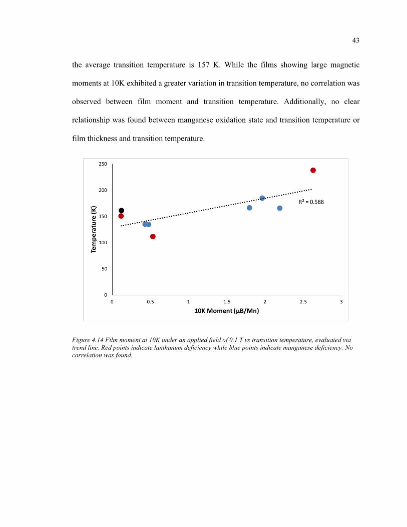
the average transition temperature is 157 K. While the films showing large magnetic

moments at 10K exhibited a greater variation in transition temperature, no correlation was

observed between film moment and transition temperature. Additionally, no clear

relationship was found between manganese oxidation state and transition temperature or

film thickness and transition temperature.

Figure 4.14 Film moment at 10K under an applied field of 0.1 T vs transition temperature, evaluated via trend line. Red points indicate lanthanum deficiency while blue points indicate manganese deficiency. No correlation was found.

R²=0.588

0

50

100

150

200

250

0 0.5 1 1.5 2 2.5 3

Tempe

rature(K

)

10KMoment(μB/Mn)

44

Figure 4.15 Manganese oxidation state vs transition temperature. Red points indicate lanthanum deficiency while blue points indicate manganese deficiency. Oxidation state determined assuming 3 oxygens of valence -2 and lanthanum of valence +3. No correlation was found.

Figure 4.16 Film thickness vs transition temperature. Red points indicate lanthanum deficiency while blue points indicate manganese deficiency. Thickness determined from x-ray reflectivity; number of unit cells based on a lattice parameter of 3.905 Å. No correlation was found.

R²=0.08298

0

50

100

150

200

250

3 3.1 3.2 3.3 3.4 3.5 3.6 3.7 3.8 3.9 4

Tran

sitionTempe

rature(K

)

ManganeseOxidationState

R²=0.021

0

50

100

150

200

250

0 20 40 60 80 100 120 140

TransitionTemperature(K

)

FilmThickness(UC)

45

Annealing

Figure 4.17 Film moment vs temperature for a constant applied field of 0.1 T, following annealing in ozone at 200 0C for 1h. Pre-anneal behavior is shown as open circles. The apparent smaller moment in several films is due to a much higher room temperature film moment, which was subtracted out as described in the experimental section.

Annealing in ozone had no appreciable effect on the moment vs. temperature

behavior of the films analyzed. However, several films showed a much higher room

temperature magnetic moment following this annealing step. This is inconsistent with

findings that oxidizing the films causes a dramatic increase in transition temperature. One

potential explanation for this is that the films were already fully oxidized, as discussed in

the previous section.

0

0.5

1

1.5

2

2.5

3

0 50 100 150 200 250 300

Film

Mom

entμ

B/Mn

Temperature(K)

MS123Oz

MS121Oz

MS138Oz

MS154Oz

0

0.1

0.2

0.3

0.4

0.5

0.6

0 50 100 150 200 250 300

Film

Mom

ent(μB/M

n)

Temperature(K)

MS152Oz

MS142Oz

MS192Oz

MS170Oz

46

5. Conclusion and Future Work

A systematic study of cation-deficient lanthanum manganite thin films deposited

via molecular beam epitaxy was undertaken. The films were characterized structurally and

in terms of magnetic behavior. Four films exhibited robust ferromagnetic behavior while

six exhibited antiferromagnetic behavior. The range of manganese oxidation states

corresponding to ferromagnetic behavior, assuming all cation deficiency was accounted

for through oxidation of manganese, was consistent with the established phase diagram for

La1-xSrxMnO3, assuming, again, all charge imbalance due to the substitutional strontium

was accounted for through oxidation of manganese.

Some unexpected behavior was seen in the lanthanum-deficient films, including an

antiferromagnetic sample which should have been within the range of ferromagnetic

samples and a sample showing a magnetic moment of more than 4 µB/Mn, assuming all

contributions to the moment were due to the manganese atoms. This could be explained

through the presence of a secondary Mn+2Mn+3O3 phase, in which manganese takes the

role of an A-site substitutional group, or phase separation into two phases with radically

different oxidation states of the manganese atom. Future studies should be done to

determine the relative stability of lanthanum vacancies and manganese substitutions, as

well as directly observe the oxidation state of the manganese in these films.

Annealing the films in an oxidizing environment showed a consistent increase in

their magnetic moment, consistent with the hypothesis that oxygen vacancies are an

alternative means of charge-balancing this material which suppresses the ferromagnetism

present in cation-deficient films. However, the change in magnetic moment was generally

47

minimal, suggesting cation composition is still the most important factor at play when

determining the magnetic behavior of these films, and that the as-grown films were already

nearly fully oxidized.

48

Works Cited

[1] C. Walter, "Kryder's Law," Scientific American, 1 August 2005.

[2] D. Rosenthal, "DSHR's Blog," 2 4 2014. [Online]. Available: http://blog.dshr.org/2014/04/evercloud-workshop.html.

[3] P. McCray, "Leaping Robot Blog," 4 2014. [Online]. Available: http://www.patrickmccray.com/2014/04/.

[4] S. Piramanayagam, "Perpendicular Recording Media for Hard Disk Drives," Journal of Applied Physics, vol. 102, p. 011301, 2007.

[5] J. J. Peng et. al., "Restoring the magnetism of ultrathin LaMnO3 films by surface symmetry engineering," Physical Review B, vol. 94, no. 214404, pp. 1-6, 2016.

[6] C. Kittel, Introduction to Solid State Physics, 8th Edition, Wiley, 2005.

[7] Y. Ren et. al., "Temperature-induced magnetization reversal in a YVO3 single crystal," Nature, vol. 396, pp. 441-444, 1998.

[8] A. Bhattacharya and S. J. May, "Magnetic Oxide Heterostructures," Annu. Rev. Mater. Res., vol. 44, pp. 65-90, 2014.

[9] M. A. Peña and J. L. G. Fierro, "Chemical Structures and Performance of Perovskite Oxides," Chem. Rev., vol. 101, pp. 1981-2017, 2001.

[10] J. Roqueta et. al., "Strain-Engineered Ferromagnetism in LaMnO3 Thin Films," Crystal Growth & Design, vol. 15, no. 11, pp. 5332-5337, 2015.

[11] G. Matsumoto, "Study of (La1-xCax)MnO3. I. Magnetic Structure of LaMnO3," Journal of the Physical Society of Japan, vol. 29, no. 3, pp. 606-614.

[12] O. H. Hansteen et. al., "Divalent manganese in reduced LaMnO3−δ—effect of oxygen nonstoichiometry on structural and magnetic properties," Solid State Sciences, vol. 6, pp. 279-285, 2004.

49

[13] J. Töpfer and J. B. Goodenough, "LaMnO3+δ Revisited," Journal of Solid State Chemistry, vol. 130, pp. 117-128, 1997.

[14] F. J. Palomares et. al., "Temperature dependence of the magnetic properties in LaMnO3+δ," Journal of Applied Physics, vol. 99, p. 08A702, 2006.

[15] C. Ritter et. al., "Influence of oxygen content on the structural, magnetotransport, and magnetic properties of LaMnO3+δ," Physical Review B, vol. 56, no. 14, pp. 8902-8911, 1997.

[16] X. Renshaw Wang et. al., "Imaging and control of ferromagnetism in LaMnO3/SrTiO3 heterostructures," Science, vol. 349, no. 6249, pp. 716-719, 2015.

[17] W. S. Choi et. al., "Effects of oxygen-reducing atmosphere annealing on LaMnO3 epitaxial thin films," Journal of Physics D: Applied Physics, vol. 42, p. 165401, 2009.

[18] W. S. Choi et. al., "LaMnO3 Thin Films Grown by Using Pulsed Laser Deposition and Their Simple Recovery to a Stoichiometric Phase by Annealing," Journal of the Korean Physical Society, vol. 58, no. 3, pp. 569-574, 2011.

[19] H. S. Kim and H. M. Christen, "Controlling the magnetic properties of LaMnO3 thin films on SrTiO3(100) by deposition in a O2/Ar gas mixture," Journal of Physics: Condensed Matter, vol. 22, p. 146007, 2010.

[20] K. H. Ahn and A. J. Millis, "Effects of in-plane strain on orbital ordering and magnetism in LaMnO3 thin film," Physica B, Vols. 312-313, pp. 766-768, 2002.

[21] A. Galdi et. al., "Magnetic properties and orbital anisotropy driven by Mn2+ in nonstoichiometric LaxMnO3−δ thin films," Physical Review B, vol. 83, no. 064418, pp. 1-7, 2011.

[22] A. Gupta et. al., "Growth and giant magnetoresistance properties of La-deficient LaxMnO3-δ (0.67<x<1) films," Applied Physics Letters, vol. 67, no. 23, pp. 3494-3496, 1995.

[23] M. Björck, "GenX," 18 10 2016. [Online]. Available: http://genx.sourceforge.net/.

[24] X. Renshaw Wang et. al., "Imaging and control of ferromagnetism in LaMnO3/SrTiO3 heterostructures," Science, vol. 349, no. 6249, pp. 716-719, 2015.

[25] V. Skumryev et. al., "Weak ferromagnetism in LaMnO3," The European Physical Journal B, vol. 11, pp. 401-406, 1999.

50

[26] S. J. Kim et. al., "Influence of La defect on the magnetoresistance and magnetic properties of La1-xMnO3," Journal of Applied Physics, vol. 89, no. 11, pp. 7416-7418, 2001.

[27] Y. Tokura and N. Nagaosa, "Physics in Transition-Metal Oxides," Science, vol. 288, no. 5465, p. 462, 2000.

[28] O. Chmaissem et. al., "Structural and magnetic phase diagrams of La1-xSrxMnO3 and Pr1-ySryMnO3," Physical Review B, vol. 67, p. 094431, 2003.