control of laser-plasma instabilities in high energy … the beam spatial profile and turn the laser...
TRANSCRIPT

Control of Laser-Plasma Instabilities in High Energy Density Plasmas Using Sub-Picosecond, High-Contrast, Temporal Modulations and Spatial Speckle-Pattern Scrambling: STUD Pulses to the Rescue
Ben Estacio, Stanford University
Bedros AfeyanPolymath Research Inc.
Stefan HüllerEcole PolytechniqueBradly Shadwick
U. Nebraska-Lincoln
PolymathResearch Inc.
pe2 = 4 ne e2
me
e2
!c≈
1137
SSAP SymposiumNorth Bethesda Marriott
Hotel2-21-2018
Work supported by the DOE FES-NNSA Joint Program in HEDLP
STUD Pulses ProgramSSAP 2-21-2018
PolymathResearch Inc.
pe2 = 4 ne e2
me
e2
!c≈
1137Outline and Summary
• What are STUD pulses? Spike Trains of Uneven Duration and Delay• What is the STUD pulse program? Ferrari, Mercedes, Prius versions• The experimental evidence for gross LPI anomalies up and down the line• How did things get so bad on NIF? > 30% energy into LPI ~ 600 kJ.• Compare USB (Plane Wave) to RPP/SSD to STUD pulses. • Key ideas: Plasmas tend to self-organize if you imbue them with coherent energy over
long periods of time: Simple growth becomes catastrophic growth• Fool the plasma into not forming memories of continuous pumping. Kill memory
accumulation, heal previous growth spurts, spread a little growth everywhere – so notin static or very slowly varying hot spots. Scramble the beam spatial profile and turn the laser beam on and off: The Ferrari STUD pulse program
• Intersperse crossing beams by synchrony and choose which interact and scramble each other’s temporal coherence due to strong coupling SBS: The Mercedes program
• In the foot of the pulse, intersperse spikes in time between crossing beams and avoid multi-beam driven instabilities: The Prius program
• Show feasibility of all three on Jupiter & Z Beamlet with flexible STUD Pulses @ 2ω.
2

STUD Pulses ProgramSSAP 2-21-2018
PolymathResearch Inc.
pe2 = 4 ne e2
me
e2
!c≈
1137
LPI History: “Decisions and Revisionswhich a Minute Will Reverse”
3
• Laser plasma instabilities (LPI) is a domain of study in the hands of plasma physicists. Not optics, laser physics, or nonlinear optics experts. Cultural divide.
• The two fields grew together in the early 60s as lasers developed. • Plasma physicists started wondering what radio wave heating of the ionosphere
and laser heating of pellets (plasma absorption) would look like. They made a lot of mistakes and got really excited about the prospect of externally controllable and tight focusable rapid heating. In each of the 3 patents of the laser, fusion by laser heating is mentioned as a key application. They had NO IDEA at the time just how it could happen.
• The field of nonlinear optics of plasmas got into full gear by 1972 and Rosenbluth’sseminal PRLs saying nonlinear wave-wave interactions will give rise to amplifiersand oscillators that may kill you. The modeling of the laser was trivialized and plasma folks used this new ICF/IFE prospect to work on plasma models with trivial laser models searching for magic tricks like staying below threshold(ill defined and impossible in practice) in paper after paper for decades!
• When laser technology changed, no reflection of same penetrated into the plasmacommunity in earnest. They were busy with their toy models and solving no pressing problem like 30% reflectivity of 2 MJ on NIF. NIF kept shooting…

STUD Pulses ProgramSSAP 2-21-2018
PolymathResearch Inc.
pe2 = 4 ne e2
me
e2
!c≈
1137
Hohlraums Contain Plasmas at Different Conditions (ne, Te, u, fe(v)) in Different locations at Different Times, Made of He, Be, CH, C, Ne, SiO2, U, Au, …
4
Non of the plasma conditions or interaction modalities that are manifest on the NIF were ever accessed on Nova or Omega.
It’s all different and yet It remains weakly characterized, weakly diagnosed, and studied only in passing.
NIF has Pdrive > 100 MB, and has achieved PStag > 150 – 200 GB but needs PStag > 300 GB to ignite at < 2 MJ.
A NIF Hohlraumis a Laser-PlasmaInstability (LPI)Candy Store

STUD Pulses ProgramSSAP 2-21-2018
PolymathResearch Inc.
pe2 = 4 ne e2
me
e2
!c≈
1137
Adequate Stringent Control of Laser-Plasma Instabilities Is Required to Achieve Indirect or Direct Drive Ignition
• Energy coupling should be > 90% to achieve high enough Trad
• Implosion symmetry requirescontrolled power balance between
“inner” and “outer” beams. Soft X-ray flux on equator vs. poles in space and time must be maintained.
• Must have low capsule preheat (Thot, fhot)
• Must control SBS, SRS, & filamentation, cross-beam energy transfer (CBET), hot electron and hard X ray (M Band) proliferation.
inner beams (l0)
outer beams (l0 +Δl)
x-beam transfer
SRS
SBS
2ωp
5
2ω p

STUD Pulses ProgramSSAP 2-21-2018
PolymathResearch Inc.
pe2 = 4 ne e2
me
e2
!c≈
1137
What Does a Laser’s Electric Field Look Like?What Are its Degrees of Freedom?
6
• Polarization• Amplitude• Wavelength• Frequency• Phase
E0 (x,t) = 1
2ei a0,slow, i (x,t)× exp ki i x −ω i t( )t +φi( )
i∑ + c.c.
If you do not like too much coherence, what are you better off modulating?
What is most likely to disrupt resonant 3 wave instability growth?
Slight changes in frequency? Phase modulations? Polarization changes?
No. The only truly effective way is via turning the amplitude of the pump wave on and off on the instability growth time scale.
What do you mean off? Contrast of 100 or better should do the trick.

STUD Pulses ProgramSSAP 2-21-2018
PolymathResearch Inc.
pe2 = 4 ne e2
me
e2
!c≈
1137
More is Different in x & t: Plasmas Self-Organizein the Presence of Coherent Energy Injection
7
SHSLong Time
Montgomery 2002
SHSShort TimeKline 2007
RPP BeamLong Time
Montgomery 1998
RPPShorter TimeBaldis 1993
STUD Pulses ProgramSSAP 2-21-2018
PolymathResearch Inc.
pe2 = 4 ne e2
me
e2
!c≈
1137
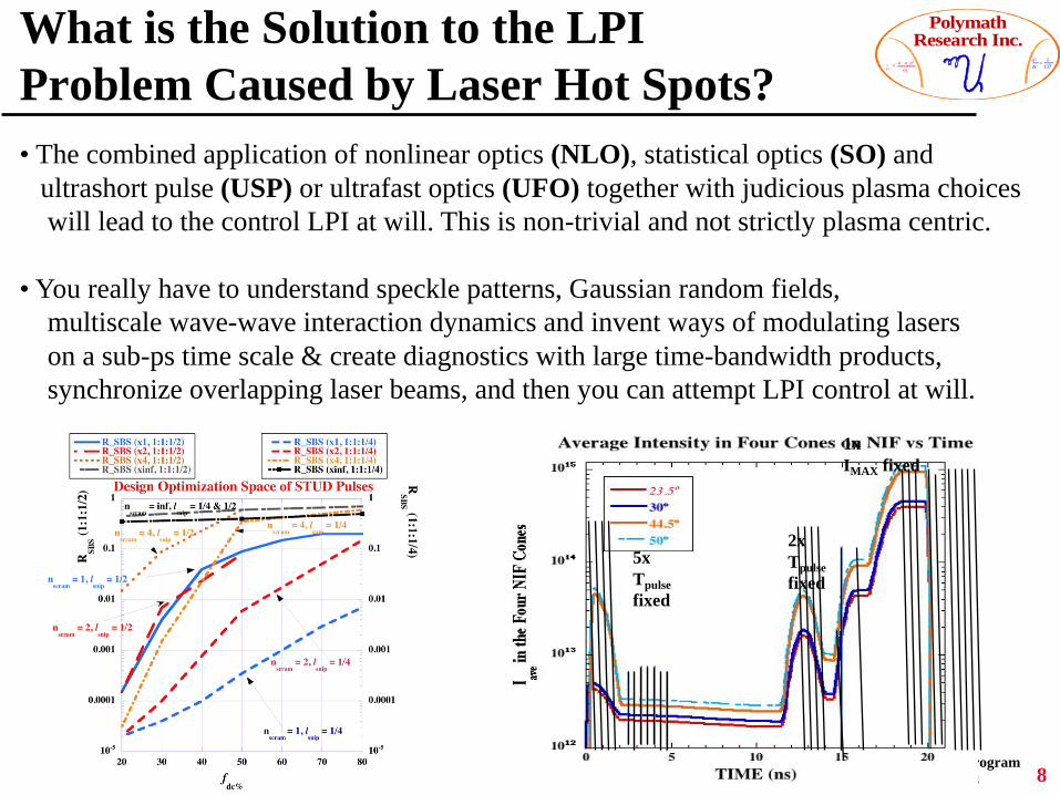
What is the Solution to the LPI Problem Caused by Laser Hot Spots?
8
• The combined application of nonlinear optics (NLO), statistical optics (SO) and ultrashort pulse (USP) or ultrafast optics (UFO) together with judicious plasma choiceswill lead to the control LPI at will. This is non-trivial and not strictly plasma centric.
• You really have to understand speckle patterns, Gaussian random fields, multiscale wave-wave interaction dynamics and invent ways of modulating laserson a sub-ps time scale & create diagnostics with large time-bandwidth products, synchronize overlapping laser beams, and then you can attempt LPI control at will.
1xIMAX fixed
2xTpulsefixed
5xTpulsefixed

STUD Pulses ProgramSSAP 2-21-2018
PolymathResearch Inc.
pe2 = 4 ne e2
me
e2
!c≈
1137The Experimental Program
• Single Hot Spot Experiments on Jupiter (with different f/#s), going beyond Montgomery/Kline/Rousseau results. Measure via OUFTS and backscattered light with sub-ps time resolution but with a long record length (100s of ps) how plasmas self-organize in SBS rich and SRS rich conditions. Various regimes, with a without FIL, SCR, SDL, WDL, WCR, large kλD, small kλD, etc.
• Witness and Capture plasma Self-Organization in action: More is different. Wait long enough and/or have a large enough plasma and reductionism becomes wishful thinking. 1-2 ps teach you very little. Look beyond single pass gain.
• Introduce STUD pulses into the mix. Solve the excesses caused by RPP/SSD/ intensity tails beyond the average intensity toy model (plane wave) picture. Jupiter, Z-Beamlet, Omega + Omega EP, Enable 2ω NIF
• Start with the rattle plate method of generating inflexible STUD pulses as pioneered by LANL (Randy Johnson and David Montgomery). Shake down Jupiter’s readiness for such expt’s. Fast diagnostics, etc.
• Move to SPA ACE flexible STUD pulse generation + CBET Control 9

STUD Pulses ProgramSSAP 2-21-2018
PolymathResearch Inc.
pe2 = 4 ne e2
me
e2
!c≈
1137
Theoretical and Computational Program• Study single hot spot long time behavior with a multitude of models
from fluid (pf3d) to Vlasov. Long time means avoid PIC categorically. • Include multitude of waves and memory accumulation after 10’s to
100’s of SHS traversal times. Study both SRS and SBS in different regimes.
• Demonstrate conditions needed for self-organization beyond the single pass gain picture. More is different? Prove it!
• Move on to large beams in 2D and 3D. Establish how much self-organization is possible in situ over long times. Now compare to large spatial self-organization and re-amplification scenarios. Work with pf3d. Add STUD pulses.
• Extract the coherent overlap fractions of re-amplification for in situ or distributed settings. The “ε”s in the formulas below.
• Concentrate on SCR, WDL of SBS for the Mercedes program: SiO2. Compare to He, CH, Ne. Add STUD pulses (w and w/o).
10
STUD Pulses ProgramSSAP 2-21-2018
PolymathResearch Inc.
pe2 = 4 ne e2
me
e2
!c≈
1137
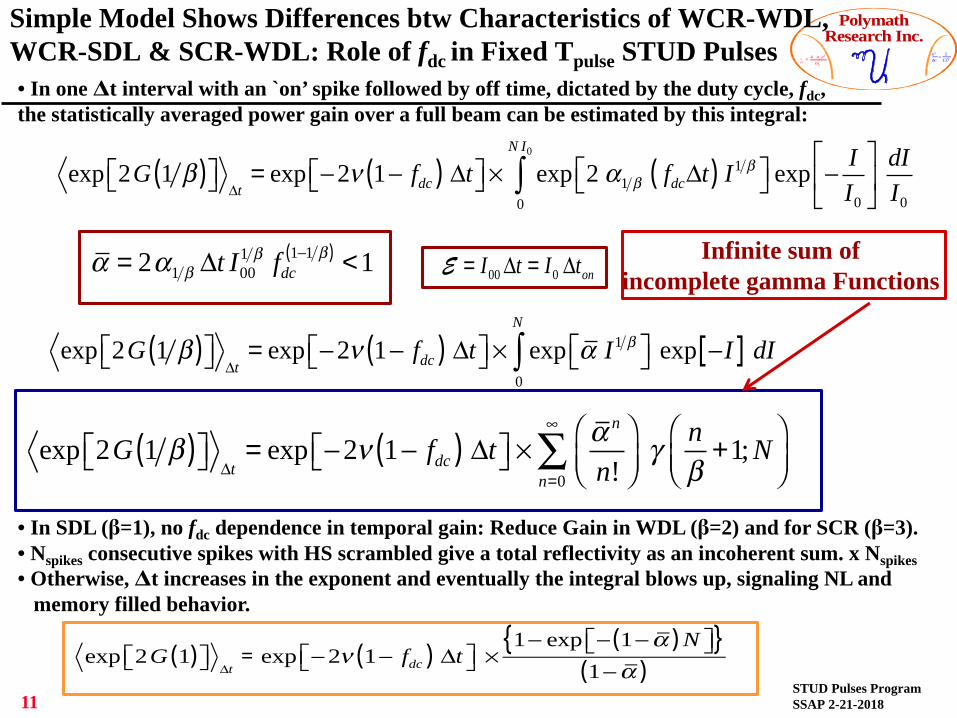
Simple Model Shows Differences btw Characteristics of WCR-WDL, WCR-SDL & SCR-WDL: Role of fdc in Fixed Tpulse STUD Pulses
11
• In one Δt interval with an `on’ spike followed by off time, dictated by the duty cycle, fdc,the statistically averaged power gain over a full beam can be estimated by this integral:
α = 2α1 β Δt I001 β fdc
1−1 β( ) <1
exp 2G 1 β( )⎡⎣ ⎤⎦ Δt= exp −2ν 1− fdc( ) Δt⎡⎣ ⎤⎦ × exp 2 α1 β fdcΔt( ) I1 β⎡⎣ ⎤⎦
0
N I0
∫ exp − II0
⎡
⎣⎢
⎤
⎦⎥
dII0
exp 2G 1 β( )⎡⎣ ⎤⎦ Δt= exp −2ν 1− fdc( ) Δt⎡⎣ ⎤⎦ × exp α I1 β⎡⎣ ⎤⎦
0
N
∫ exp −I[ ] dI
• In SDL (β=1), no fdc dependence in temporal gain: Reduce Gain in WDL (β=2) and for SCR (β=3).• Nspikes consecutive spikes with HS scrambled give a total reflectivity as an incoherent sum. x Nspikes• Otherwise, Δt increases in the exponent and eventually the integral blows up, signaling NL and
memory filled behavior.
exp 2G 1 β( )⎡⎣ ⎤⎦ Δt= exp −2ν 1− fdc( ) Δt⎡⎣ ⎤⎦ ×
α n
n!⎛⎝⎜
⎞⎠⎟n=0
∞
∑ γ nβ
+1;N⎛⎝⎜
⎞⎠⎟
E = I00Δt = I0 Δton
exp 2G 1( )⎡⎣ ⎤⎦ Δt= exp −2ν 1− fdc( ) Δt⎡⎣ ⎤⎦ ×
1− exp − 1−α( )N⎡⎣ ⎤⎦{ }1−α( )
Infinite sum of incomplete gamma Functions

STUD Pulses ProgramSSAP 2-21-2018
PolymathResearch Inc.
pe2 = 4 ne e2
me
e2
!c≈
1137
A Theoretical Model Captures These Anomalies Showing How STUD Pulses Lead to Taming and Control
12
Memory buildup in time and in space à More is different.
Triggers: Out of equilibrium kinetic effects, nonlinearity, absolute instability, localized modes, feedback loops
STUD pulses: lsnip = ½ makes G smaller. nscram = 1 tames fastest. fdc helps stack/intersperse beams and heal via damping between growth spurts.
Fool the plasma and dissuade it from expecting same or hotter hot spots coming to the same place. Stop memory build-up, heal, democratize or homogenize gain in (x, t). TAME instabilities.
RUSB = δnn 0
eG Iave( ) + ε2e2G Iave( ) + ...+ εNsat
eNsat G Iave( )⎡⎣
⎤⎦ + IS 0
eG Iave( )
RRPP = δnn 0
eG I( ) + ε2e2G I( ) + ...+ εNsat
eNsat G I( )⎡⎣
⎤⎦
0
IMAX
∫e−I Iave
Iave
dI + IS 0eG I( )⎡⎣ ⎤⎦
0
IMAX
∫e−I Iave
Iave
dI + δ1 eG I( )⎡⎣ ⎤⎦0
IMAX
∫e−I Iave
Iave
dI⎛
⎝⎜⎞
⎠⎟
2
+ ...⎡
⎣⎢⎢
⎤
⎦⎥⎥
RSTUD = δnn 0
eG I( )⎡⎣ ⎤⎦0
IMAX
∫e−I Iave
Iave
dI + ε2 dI1 dI2I1
IMAX
∫ eG I1( )eG I2( )⎡⎣ ⎤⎦0
IMAX
∫e− I1+I2( )
Iave
Iave
+ ...+ εN e G( I )⎡
⎣
⎢⎢⎢
⎤
⎦
⎥⎥⎥+ IS 0
eG I( )⎡⎣ ⎤⎦0
IMAX
∫e−I Iave
Iave
dI + δ1I1
IMAX
∫ dI1 dI2 eG I1( )+G I2( )⎡⎣ ⎤⎦0
IMAX
∫e− I1+I2( )
Iave
Iave
⎛
⎝
⎜⎜
⎞
⎠
⎟⎟
+ ...⎡
⎣
⎢⎢⎢
⎤
⎦
⎥⎥⎥

STUD Pulses ProgramSSAP 2-21-2018
PolymathResearch Inc.
pe2 = 4 ne e2
me
e2
!c≈
1137
Where Can STUD Pulse Design Do the Most Good in Reducing Reflectivity?
13

STUD Pulses ProgramSSAP 2-21-2018
PolymathResearch Inc.
pe2 = 4 ne e2
me
e2
!c≈
1137
What Does Memory & Gain-Guided Growth Cones inSingle (Diffraction Limited) Hot Spot SDL SBS Look Like?
14
STUD Pulses ProgramSSAP 2-21-2018
PolymathResearch Inc.
pe2 = 4 ne e2
me
e2
!c≈
1137
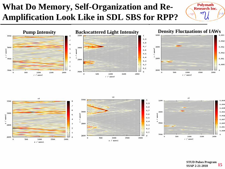
What Do Memory, Self-Organization and Re-Amplification Look Like in SDL SBS for RPP?
15
Pump Intensity Backscattered Light Intensity Density Fluctuations of IAWs
STUD Pulses ProgramSSAP 2-21-2018
PolymathResearch Inc.
pe2 = 4 ne e2
me
e2
!c≈
1137
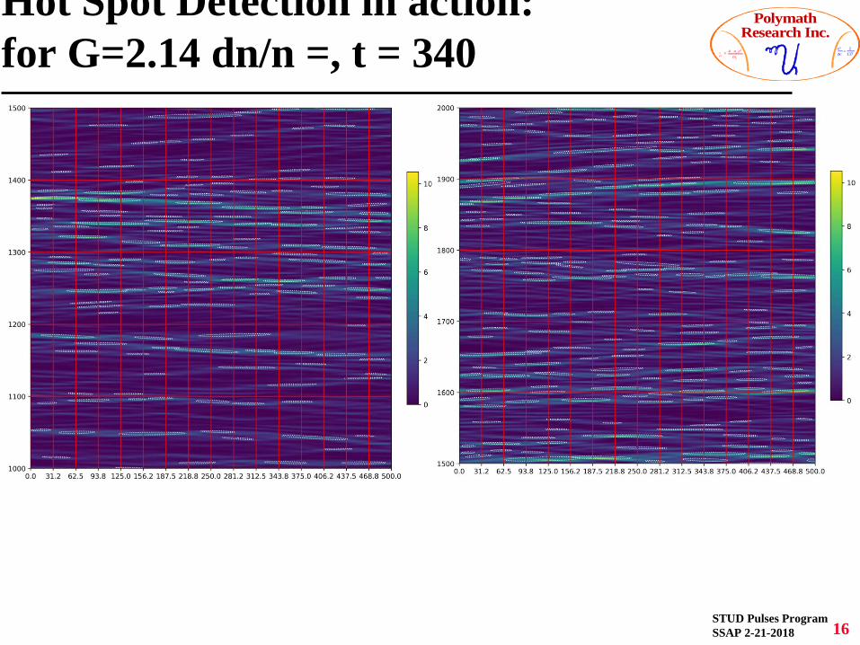
Hot Spot Detection in action: for G=2.14 dn/n =, t = 340
16

STUD Pulses ProgramSSAP 2-21-2018
PolymathResearch Inc.
pe2 = 4 ne e2
me
e2
!c≈
1137
Hot Spot Detection in action: for G=2.14 dn/n =, t = 340
17

STUD Pulses ProgramSSAP 2-21-2018
PolymathResearch Inc.
pe2 = 4 ne e2
me
e2
!c≈
1137
Statistical connections between amplification processes in various hot spots are captured via correlation functionsin (l, m, n, o, t) space
18
ρE0,S l ,m,l ',m';t( ) =E0,S l ,m,τ( )E0,S* l ',m',t +τ( )dτ
τmin
τmax∫E0,S l ,m,τ( ) 2dτ
τmin
τmax∫ E0,S l ',m',τ( ) 2dττmin
τmax∫
The Complex Degree of Coherence (CDC) of a complex field is the normalized version of the Mutual Coherence Function (MCF). Here quntized onto an ordered hot spot lattice (l,m)
Movies of MCF and CDC indicate whether initial pass tranchesand final pass tranches evolve entirely differently negating the precepts that make up the universally help view that the independent hot spot model applies when in fact, many hot spots can reamplifiedprevious gain sites in an RPP beam and reek havoc. (Think NIF/NIC)
This is what the STUD pulse program reverses.
STUD Pulses ProgramSSAP 2-21-2018
PolymathResearch Inc.
pe2 = 4 ne e2
me
e2
!c≈
1137
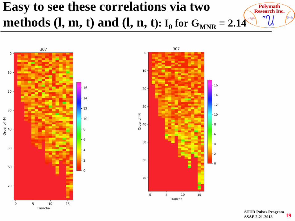
Easy to see these correlations via two methods (l, m, t) and (l, n, t): I0 for GMNR = 2.14
19
STUD Pulses ProgramSSAP 2-21-2018
PolymathResearch Inc.
pe2 = 4 ne e2
me
e2
!c≈
1137
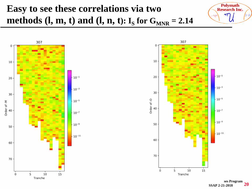
Easy to see these correlations via two methods (l, m, t) and (l, n, t): IS for GMNR = 2.14
20

STUD Pulses ProgramSSAP 2-21-2018
PolymathResearch Inc.
pe2 = 4 ne e2
me
e2
!c≈
1137
Easy to see these correlations via two methods (l, m, t) and (l, n, t): !n/n for GMNR = 2.14
21

STUD Pulses ProgramSSAP 2-21-2018
PolymathResearch Inc.
pe2 = 4 ne e2
me
e2
!c≈
1137
Mutual Coherence Function for ISfor GMNR = 2.14 and dn/n 1e-9
22
STUD Pulses ProgramSSAP 2-21-2018
PolymathResearch Inc.
pe2 = 4 ne e2
me
e2
!c≈
1137
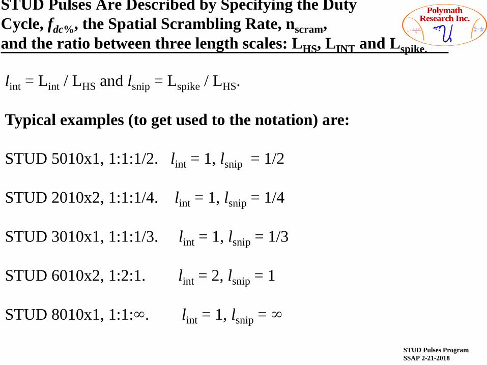
STUD Pulses Are Described by Specifying the DutyCycle, fdc%, the Spatial Scrambling Rate, nscram, and the ratio between three length scales: LHS, LINT and Lspike.
lint = Lint / LHS and lsnip = Lspike / LHS.
Typical examples (to get used to the notation) are:
STUD 5010x1, 1:1:1/2. lint = 1, lsnip = 1/2
STUD 2010x2, 1:1:1/4. lint = 1, lsnip = 1/4
STUD 3010x1, 1:1:1/3. lint = 1, lsnip = 1/3
STUD 6010x2, 1:2:1. lint = 2, lsnip = 1
STUD 8010x1, 1:1:∞. lint = 1, lsnip = ∞

STUD Pulses ProgramSSAP 2-21-2018
PolymathResearch Inc.
pe2 = 4 ne e2
me
e2
!c≈
1137
What Do STUD Pulses Look Like?
5010x∞ 1:1:1/2
5010x1 1:1:1
Harmony Simulations

STUD Pulses ProgramSSAP 2-21-2018
PolymathResearch Inc.
pe2 = 4 ne e2
me
e2
!c≈
1137
A Comparison of IPump, ISBS, δn/n|IAW for ωIAW t = 205010x16 1:1:1, 5010x16 1:1:1/2, 5010x8 1:1:1 & 5010x8 1:1:1/2. Notice Memory Loss, Democratization, Taming
STUD Pulses ProgramSSAP 2-21-2018
PolymathResearch Inc.
pe2 = 4 ne e2
me
e2
!c≈
1137
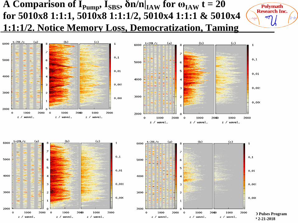
A Comparison of IPump, ISBS, δn/n|IAW for ωIAW t = 20for 5010x8 1:1:1, 5010x8 1:1:1/2, 5010x4 1:1:1 & 5010x41:1:1/2. Notice Memory Loss, Democratization, Taming

STUD Pulses ProgramSSAP 2-21-2018
PolymathResearch Inc.
pe2 = 4 ne e2
me
e2
!c≈
1137
A Comparison of IPump, ISBS, δn/n|IAW for ωIAW t = 20for 5010x4 1:1:1, 5010x4 1:1:1/2, 5010x2 1:1:1 & 5010x21:1:1/2. Notice Memory Loss, Democratization, Taming

STUD Pulses ProgramSSAP 2-21-2018
PolymathResearch Inc.
pe2 = 4 ne e2
me
e2
!c≈
1137
A Comparison of IPump, ISBS, δn/n|IAW for ωIAW t = 20for 5010x2 1:1:1, 5010x2 1:1:1/2, 5010x1 1:1:1 & 5010x11:1:1/2. Notice Memory Loss, Democratization, Taming
STUD Pulses ProgramSSAP 2-21-2018
PolymathResearch Inc.
pe2 = 4 ne e2
me
e2
!c≈
1137
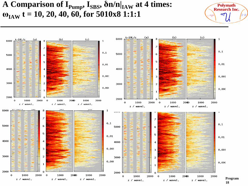
A Comparison of IPump, ISBS, δn/n|IAW at 4 times: ωIAW t = 10, 20, 40, 60, for 5010x8 1:1:1

STUD Pulses ProgramSSAP 2-21-2018
PolymathResearch Inc.
pe2 = 4 ne e2
me
e2
!c≈
1137
A Comparison of IPump, ISBS, δn/n|IAW at 3 times: ωIAW t = 10, 20, 40, for 5010x8 1:1:1/2
STUD Pulses ProgramSSAP 2-21-2018
PolymathResearch Inc.
pe2 = 4 ne e2
me
e2
!c≈
1137
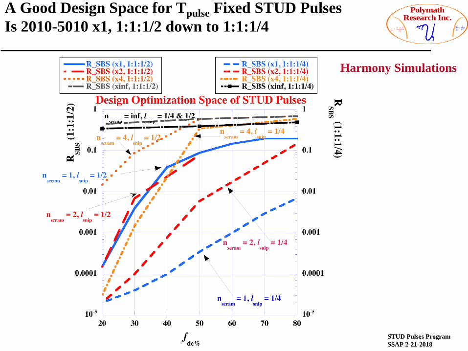
A Good Design Space for Tpulse Fixed STUD PulsesIs 2010-5010 x1, 1:1:1/2 down to 1:1:1/4
Harmony Simulations
STUD Pulses ProgramSSAP 2-21-2018
PolymathResearch Inc.
pe2 = 4 ne e2
me
e2
!c≈
1137
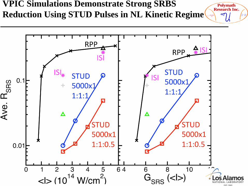
VPIC Simulations Demonstrate Strong SRBS Reduction Using STUD Pulses in NL Kinetic Regime

STUD Pulses ProgramSSAP 2-21-2018
PolymathResearch Inc.
pe2 = 4 ne e2
me
e2
!c≈
1137
Jupiter Layout for Crossed Beam STUD Pulse Expts: Observing Weak to Strong Coupling Brillouin Interactions Directly via IAW Frequency Shifts via TS and Indirectly via FABS/TBD
33
SiO2 AerogelFoam
Compare Random to Deterministic STUD Pulse sequences

STUD Pulses ProgramSSAP 2-21-2018
PolymathResearch Inc.
pe2 = 4 ne e2
me
e2
!c≈
1137
Questions to Be Answered in Jupiter STUD Pulse Program, Proof of Principle Experiments
• Prius Program: Cross 2 STUD pulsed beams and monitor LPI driven by each as they overlap in time deterministically and randomly with narrow spikes and wider one from 1 to 20 ps in duration, with different off times testing 20% duty cycle to 50%. Do this in CH.
• Mercedes Program: Move to SiO2 and the SCR of CBET and SBS. Directly measure the frequency shifts of IAW in the SCR near Mach -1 or not, in hot spots or not. Vary STUD pulse characteristics as above. Correlate LPI scattered light signatures to direct OUFTS.
• In the Mercedes Program, work with one STUD pulse beam alone, then one STUS pulse beam and one continuous beam crossing, and then two STUD pulse beams partially overlapping vs fully overlapping.
• Examine scaling with f/# and RPP choices. Compare to continuous beam behavior. Vary plasma composition and conditions.
34

STUD Pulses ProgramSSAP 2-21-2018
PolymathResearch Inc.
pe2 = 4 ne e2
me
e2
!c≈
1137
How Would Findings on Jupiter Scale to NIF? (via Z-Beamlet or Ω-EP Blue)
• For NIF need single beam remediation in the foot (2ωp, SRS) and the peak (SRS, 2ωp, SBS) as well as multi-beam remediation (SRS, SBS, CBET, 2ωp) in the foot and the peak.
• These are entirely different plasma conditions (all unknown) whether low gas fill or high gas fill or intermediate gas fill.
• Confidence in random crossing fraction scaling of LPI and superiority with continuous beams overlapping will be established and should scale. It will be easy to test subsequently on NIF with a few quads equipped with STUD pulses.
• Deterministic synchronization solutions can be intimately coupled to plasma conditions which are very different between Trident and NIF.
• One step is to go to Omega EP Blue/Green Beams brought over to Omega and equipped with STUD pulses to do LPI experiments on Omega with STUD pulses en attendant NIF. Random synchronization is easiest scenario to test on Omega EP + Omega and for DD applications.
35

STUD Pulses ProgramSSAP 2-21-2018
PolymathResearch Inc.
pe2 = 4 ne e2
me
e2
!c≈
1137
SBS & CBET Represent a Specific Example Where We Can Derive Such Equations
∂∂t
+ u(x) i∇ +ν IAW⎛⎝⎜
⎞⎠⎟
∂∂t
+ u(x) i∇⎛⎝⎜
⎞⎠⎟ − cs
2∇2⎡⎣⎢
⎤⎦⎥δne
n( )
n0
= Z me
M I
⎛⎝⎜
⎞⎠⎟∇2 u0
n( ) i usn( )( ) + cs kIAW( )2 δne
n−1( )
n0
∂2
∂t 2 − c2∇2 +ω p2 x( ) 1− ν s
ω s
⎛⎝⎜
⎞⎠⎟
⎡
⎣⎢
⎤
⎦⎥us
n( ) = −ω p2 δne
n( )
n0
u0n( ) +ω s
2 usn−1( )
∂2
∂t 2 − c2∇2 +ω p2 x( ) 1− ν0
ω 0
⎛⎝⎜
⎞⎠⎟
⎡
⎣⎢
⎤
⎦⎥u0
n( ) = −ω p2 δne
n( )
n0
usn( ) +ω 0
2 u0n−1( )
Use electromagnetic units and extract the eikonal “fast” variables to leave the interaction physics living atop travelling waves.
δnen( )
n0
x,t( ) =α δ !n*e
n( )
n0
x,t( )exp −i k IAW i dx∫ −ω IAW t( )⎡⎣
⎤⎦
usn( ) x,t( ) = β u0 !us
n( ) x,t( ) exp i ks i dx∫ −ω st( )⎡⎣
⎤⎦
u0n( ) x,t( ) = γ u0
!u0n( )
2x,t( ) exp i k0 i x∫ −ω 0t( )⎡
⎣⎤⎦ + cc.

STUD Pulses ProgramSSAP 2-21-2018
PolymathResearch Inc.
pe2 = 4 ne e2
me
e2
!c≈
1137
Including All Regimes in IAW Response for SBS Evolution in Inhomogeneous Flowing Plasma
∂∂t
+ ν IAW (x)2
+ cs M(x)+ k IAW⎡⎣ ⎤⎦ i∇⎛⎝⎜
⎞⎠⎟− i
2cs
∂∂t
+ cs
cM(x) i∇⎛
⎝⎜⎞⎠⎟
2
− cs2∇2⎡
⎣⎢
⎤
⎦⎥
⎡
⎣⎢⎢
⎤
⎦⎥⎥
δ !n*e
n( )
n0
= iγ 0 eiδω tus(n) − i cs
2δ !n*
en−1( )
n0
∂∂t
+ ν s (x)2
−Vs i∇⎡⎣⎢
⎤⎦⎥+ i
2ω s
∂2
∂t 2 −∇2⎡
⎣⎢
⎤
⎦⎥ !us
n( ) = −iγ 0 e− iδω t δ !n*e
n( )
n0
+ − iω s
2!us
n−1( )
ν IAW (x) = ν IAW
cs kIAW
⎛⎝⎜
⎞⎠⎟
cs
⎡
⎣⎢
⎤
⎦⎥ − 2ics x − x0( ) i∇M(x)⎡⎣ ⎤⎦ i k IAW⎡⎣ ⎤⎦
ν s (x) =ω p
2
ω 02
ν s
ω s
⎛⎝⎜
⎞⎠⎟
+ 2i x − x0( ) i∇ ln ω p2 x( )( )⎡⎣ ⎤⎦
⎡
⎣⎢
⎤
⎦⎥
γ WCR−WDL = γ 02 − 1
2ν IAW
2cs kIAW
⎛⎝⎜
⎞⎠⎟
ν s
2ω s
⎛⎝⎜
⎞⎠⎟− δω 2
4⎡
⎣⎢
⎤
⎦⎥
1/2
− ν IAW
2cs kIAW
⎛⎝⎜
⎞⎠⎟− ν s
2ω s
⎛⎝⎜
⎞⎠⎟
γ WCR−SDL =γ 0
2 ν IAW
2cs kIAW
⎛⎝⎜
⎞⎠⎟
ν IAW
2cs kIAW
⎛⎝⎜
⎞⎠⎟
2
+δω 2⎛
⎝⎜
⎞
⎠⎟
− ν s
2ω s
⎛⎝⎜
⎞⎠⎟
⎡
⎣
⎢⎢⎢⎢⎢
⎤
⎦
⎥⎥⎥⎥⎥
γ SCR−WDL = cos π6
⎛⎝⎜
⎞⎠⎟ cs γ 0
2 − 12
ν IAW
2cs kIAW
⎛⎝⎜
⎞⎠⎟
ν s
2ω s
⎛⎝⎜
⎞⎠⎟− δω 2
4⎡
⎣⎢
⎤
⎦⎥
⎧⎨⎪
⎩⎪
⎫⎬⎪
⎭⎪
1/3
γ 02
ω 02 = 1
8Z me
M I
⎛⎝⎜
⎞⎠⎟
u0
c⎛⎝⎜
⎞⎠⎟
2 ω p2
ω 02
⎛
⎝⎜⎞
⎠⎟kIAW k0( )2
cs c( ) kIAW k0( )⎡⎣ ⎤⎦
γ 02
ω 02 = 4.1835 ×10⁻⁸ 2Z
A⎛⎝⎜
⎞⎠⎟
1 2 ne nc
0.1⎡⎣⎢
⎤⎦⎥
2sin θ s 2( )⎡⎣ ⎤⎦I
14, W /cm2λ0,0.351µm2
Te. keV
u0
c⎛⎝⎜
⎞⎠⎟
2
= 8.9712 ×10⁻⁶ I14, W /cm2λ0,0.351µm
2
cs
c⎛⎝⎜
⎞⎠⎟ = 7.3×10⁻⁴ 2Z
A⎛⎝⎜
⎞⎠⎟
1 2
Te. keV
cs = cs c( ) kIAW k0( )⎡⎣ ⎤⎦ = 7.3×10⁻⁴ 2ZA
⎛⎝⎜
⎞⎠⎟
1 2
Te. keV 2sin θ s 2( )⎡⎣ ⎤⎦
ω 0 Δt ps( ) = 5.3702 ×10³
λ0,0.351µm
Δt ps
STUD Pulses ProgramSSAP 2-21-2018
PolymathResearch Inc.
pe2 = 4 ne e2
me
e2
!c≈
1137
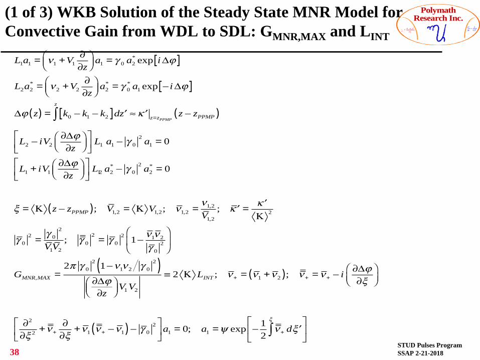
(1 of 3) WKB Solution of the Steady State MNR Model for Convective Gain from WDL to SDL: GMNR,MAX and LINT
38
L1a1 = ν1 +V1∂∂z
⎛⎝⎜
⎞⎠⎟ a1 = γ 0 a2
* exp iΔϕ[ ]
L2a2* = ν2 +V2
∂∂z
⎛⎝⎜
⎞⎠⎟ a2
* = γ 0* a1 exp − iΔϕ[ ]
Δϕ z( ) = k0 − k1 − k2[ ]z
∫ d ′z ≈ ′κ z=zPPMPz − zPPMP( )
L2 − iV2∂Δϕ∂z
⎛⎝⎜
⎞⎠⎟
⎡⎣⎢
⎤⎦⎥
L1 a1 − γ 02 a1 = 0
L1 + iV1∂Δϕ∂z
⎛⎝⎜
⎞⎠⎟
⎡⎣⎢
⎤⎦⎥
L12 a2* − γ 0
2 a2* = 0
ξ = Κ z − zPPMP( ); V1,2 = Κ V1,2; ν1,2 =ν1,2
V1,2
; ′κ = ′κΚ 2
γ 02 =
γ 02
V1V2
; γ 02
= γ 02 1− ν1ν2
γ 02
⎛
⎝⎜
⎞
⎠⎟
GMNR,MAX =2π γ 0
2 1−ν1ν2 γ 02( )
∂Δϕ∂z
⎛⎝⎜
⎞⎠⎟V1V2
≡ 2 Κ LINT ; ν+ = ν1 +ν2( ); ν+ =ν+ − i ∂Δϕ∂ξ
⎛⎝⎜
⎞⎠⎟
∂2
∂ξ 2 +ν+∂∂ξ
+ν1 ν+ −ν1( )− γ 02⎡
⎣⎢
⎤
⎦⎥a1 = 0; a1 =ψ exp − 1
2ν+ d ′ξ
ξ
∫⎡
⎣⎢
⎤
⎦⎥
STUD Pulses ProgramSSAP 2-21-2018
PolymathResearch Inc.
pe2 = 4 ne e2
me
e2
!c≈
1137
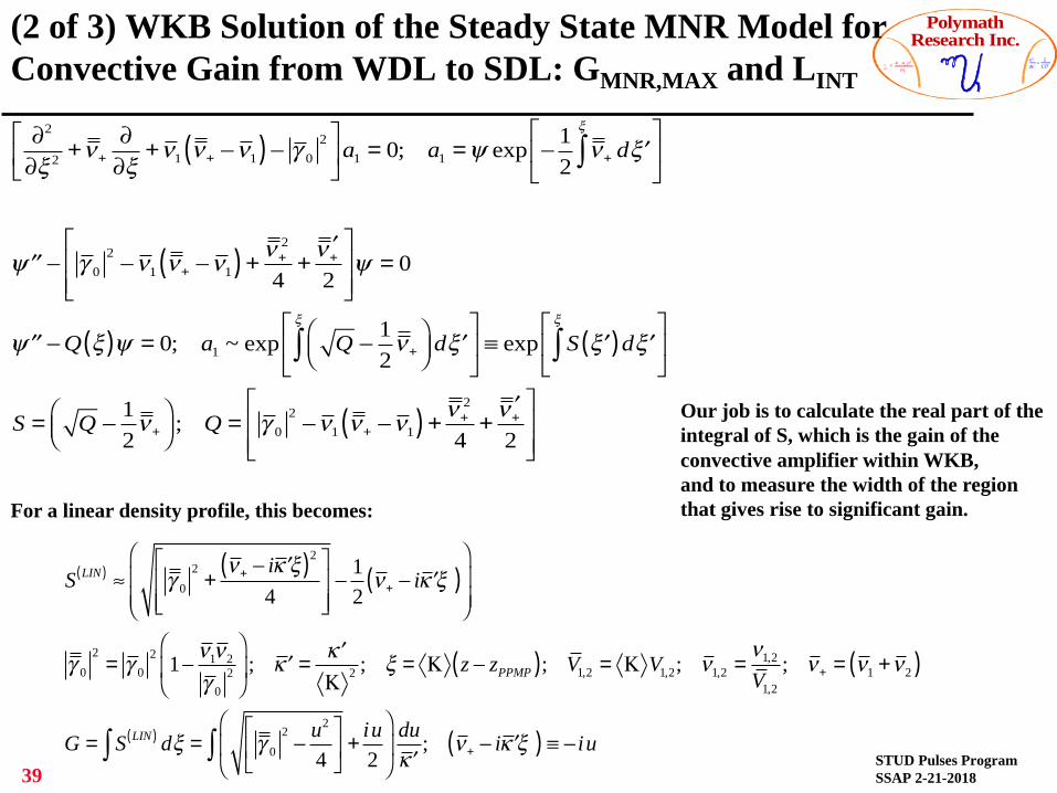
(2 of 3) WKB Solution of the Steady State MNR Model for Convective Gain from WDL to SDL: GMNR,MAX and LINT
39
∂2
∂ξ 2 +ν+∂∂ξ
+ν1 ν+ −ν1( )− γ 02⎡
⎣⎢
⎤
⎦⎥a1 = 0; a1 =ψ exp − 1
2ν+ d ′ξ
ξ
∫⎡
⎣⎢
⎤
⎦⎥
′′ψ − γ 02 −ν1 ν+ −ν1( ) + ν+
2
4+ ν+
′2
⎡
⎣⎢⎢
⎤
⎦⎥⎥ψ = 0
′′ψ −Q ξ( )ψ = 0; a1 ~ exp Q − 12ν+
⎛⎝⎜
⎞⎠⎟ d ′ξ
ξ
∫⎡
⎣⎢
⎤
⎦⎥ ≡ exp S ′ξ( )d ′ξ
ξ
∫⎡
⎣⎢
⎤
⎦⎥
S = Q − 12ν+
⎛⎝⎜
⎞⎠⎟ ; Q = γ 0
2 −ν1 ν+ −ν1( ) + ν+2
4+ ν+
′2
⎡
⎣⎢⎢
⎤
⎦⎥⎥
Our job is to calculate the real part of theintegral of S, which is the gain of theconvective amplifier within WKB,and to measure the width of the region that gives rise to significant gain. For a linear density profile, this becomes:
S LIN( ) ≈ γ 02
+ν+ − i ′κ ξ( )2
4⎡
⎣⎢⎢
⎤
⎦⎥⎥− 1
2ν+ − i ′κ ξ( )
⎛
⎝⎜⎜
⎞
⎠⎟⎟
γ 02
= γ 02 1− ν1ν2
γ 02
⎛
⎝⎜
⎞
⎠⎟ ; ′κ = ′κ
Κ 2 ; ξ = Κ z − zPPMP( ); V1,2 = Κ V1,2; ν1,2 =ν1,2
V1,2
; ν+ = ν1 +ν2( )
G = S LIN( ) dξ∫ = γ 02− u2
4⎡
⎣⎢
⎤
⎦⎥ + iu
2
⎛
⎝⎜
⎞
⎠⎟∫
du′κ; ν+ − i ′κ ξ( ) ≡ − iu
STUD Pulses ProgramSSAP 2-21-2018
PolymathResearch Inc.
pe2 = 4 ne e2
me
e2
!c≈
1137
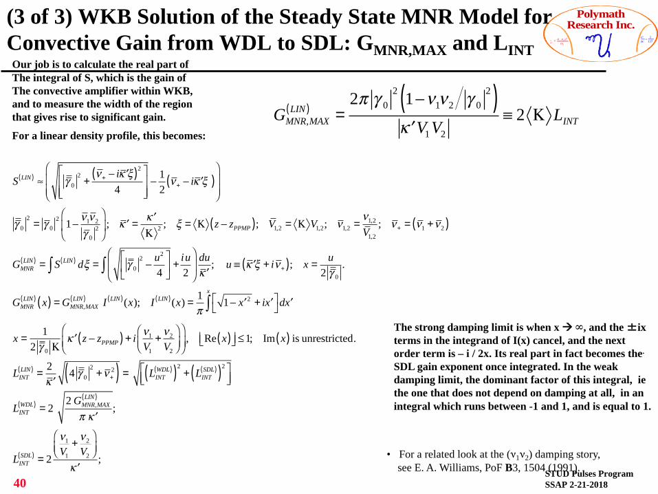
(3 of 3) WKB Solution of the Steady State MNR Model for Convective Gain from WDL to SDL: GMNR,MAX and LINT
40
Our job is to calculate the real part of The integral of S, which is the gain of The convective amplifier within WKB,and to measure the width of the region that gives rise to significant gain. For a linear density profile, this becomes:
The strong damping limit is when x à ∞, and the �ix terms in the integrand of I(x) cancel, and the next order term is – i / 2x. Its real part in fact becomes the.
SDL gain exponent once integrated. In the weak damping limit, the dominant factor of this integral, iethe one that does not depend on damping at all, in an integral which runs between -1 and 1, and is equal to 1.
• For a related look at the (ν1ν2) damping story, see E. A. Williams, PoF B3, 1504 (1991).
S LIN( ) ≈ γ 02
+ν+ − i ′κ ξ( )2
4⎡
⎣⎢⎢
⎤
⎦⎥⎥− 1
2ν+ − i ′κ ξ( )
⎛
⎝⎜⎜
⎞
⎠⎟⎟
γ 02
= γ 02 1− ν1ν2
γ 02
⎛
⎝⎜
⎞
⎠⎟ ; ′κ = ′κ
Κ 2 ; ξ = Κ z − zPPMP( ); V1,2 = Κ V1,2; ν1,2 =ν1,2
V1,2
; ν+ = ν1 +ν2( )
GMNRLIN( ) = S LIN( ) dξ∫ = γ 0
2− u2
4⎡
⎣⎢
⎤
⎦⎥ + iu
2
⎛
⎝⎜
⎞
⎠⎟∫
du′κ; u ≡ ′κ ξ + iν+( ); x = u
2 γ 0
.
GMNRLIN( ) x( ) = GMNR,MAX
LIN( ) I LIN( )(x); I LIN( )(x) = 1π
1− ′x 2 + i ′x⎡⎣
⎤⎦d ′x
x
∫
x = 12 γ 0 Κ
′κ z − zPPMP( ) + i ν1
V1
+ ν2
V2
⎛⎝⎜
⎞⎠⎟
⎛
⎝⎜⎞
⎠⎟, Re x( )⎢⎣ ⎥⎦ ≤1; Im x( ) is unrestricted.
LINTLIN( ) = 2
′κ4 γ 0
2+ν+
2( ) = LINTWDL( )( )2
+ LINTSDL( )( )2⎡
⎣⎢⎤⎦⎥
LINTWDL( ) = 2
2 GMNR,MAXLIN( )
π ′κ;
LINTSDL( ) = 2
ν1
V1
+ ν2
V2
⎛⎝⎜
⎞⎠⎟
′κ;
GMNR,MAXLIN( ) =
2π γ 02 1−ν1ν2 γ 0
2( )′κ V1V2
≡ 2 Κ LINT

STUD Pulses ProgramSSAP 2-21-2018
PolymathResearch Inc.
pe2 = 4 ne e2
me
e2
!c≈
1137
Besides the Gain Exponent, A Crucial Quantity Is the Gain Length Which Varies between SDL, WDL, SCL, WCL, SRS, SBS
LINTWDL( ) = 2
V2
ω2
⎛⎝⎜
⎞⎠⎟
dk2
dz⎛⎝⎜
⎞⎠⎟
⎡
⎣
⎢⎢⎢⎢
⎤
⎦
⎥⎥⎥⎥
γ 0
ω0
⎛⎝⎜
⎞⎠⎟
V2
V1
⎛⎝⎜
⎞⎠⎟
ω2
ω0
⎛⎝⎜
⎞⎠⎟
⎡
⎣
⎢⎢⎢⎢⎢
⎤
⎦
⎥⎥⎥⎥⎥
LINTSDL( ) = 2
V2
ω2
⎛⎝⎜
⎞⎠⎟
dk2
dz⎛⎝⎜
⎞⎠⎟
⎡
⎣
⎢⎢⎢⎢
⎤
⎦
⎥⎥⎥⎥
ν2
ω2
⎛⎝⎜
⎞⎠⎟
⎡
⎣⎢
⎤
⎦⎥
2V2
ω2
⎛⎝⎜
⎞⎠⎟
dk2
dz⎛⎝⎜
⎞⎠⎟
⎡
⎣
⎢⎢⎢⎢
⎤
⎦
⎥⎥⎥⎥
SRBS
= 4Ln
γ 0
ω0
⎛⎝⎜
⎞⎠⎟ SRBS
= 12
v osc
c= 4.267×10⁻³ I14 λ0,µm
V2
V1
⎛⎝⎜
⎞⎠⎟
ω2
ω0
⎛⎝⎜
⎞⎠⎟
SRBS
= 7.66 ×10⁻² Te,keV
1− nnc
+ 1− 2 nnc
⎛⎝⎜
⎞⎠⎟
nnc
( )3 4
kEPWSRBSλD( ) = 4.42 ×10⁻² Te,keV
1− nnc
+ 1− 2 nnc
⎛⎝⎜
⎞⎠⎟
nnc
ν2 kEPWSRBSλD > 0.25( )
ω2
⎛
⎝⎜
⎞
⎠⎟
SRBS
= −0.23+ 2.2 kEPWSRBSλD( )− 6.6 kEPW
SRBSλD( )2+ 6.8 kEPW
SRBSλD( )3− 3.9 kEPW
SRBSλD( )4+ 0.96 kEPW
SRBSλD( )5
Design STUD pulses so that:
LSPIKE < LINT < LHS
LHS ~ 4 f2 λ0LSPIKE = tspike x Vg, scattFor Raman Backscattering, in particular:
GMNR,MAXSRBS LIN( ) =
4π γ 0
ω0
⎛⎝⎜
⎞⎠⎟
2
SRBS
2πLn
λ0
⎛⎝⎜
⎞⎠⎟
1− 2 nnc
1− nnc
⎛
⎝
⎜⎜⎜⎜⎜
⎞
⎠
⎟⎟⎟⎟⎟
nnc
⎡
⎣
⎢⎢⎢⎢⎢
⎤
⎦
⎥⎥⎥⎥⎥
STUD Pulses ProgramSSAP 2-21-2018
PolymathResearch Inc.
pe2 = 4 ne e2
me
e2
!c≈
1137
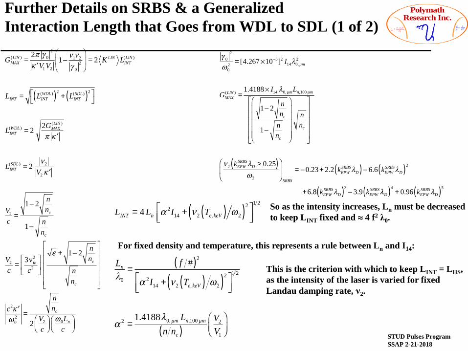
Further Details on SRBS & a Generalized Interaction Length that Goes from WDL to SDL (1 of 2)
GMAX(LIN ) =
2π γ 02
′κ V1V2
1− ν1ν2
γ 02
⎛
⎝⎜
⎞
⎠⎟ = 2 K LIN LINT
(LIN )
LINT = LINT(WDL )( )2
+ LINT(SDL )( )2⎡
⎣⎤⎦
LINT(WDL ) = 2 2GMAX
(LIN )
π ′κ
LINT(SDL ) = 2
ν2
V2 ′κ
V1
c=
1− 2 nnc
1− nnc
V2
c= 3vth
2
c2
⎡
⎣⎢
⎤
⎦⎥
ε + 1− 2 nnc
nnc
⎡
⎣
⎢⎢⎢⎢⎢
⎤
⎦
⎥⎥⎥⎥⎥
c2 ′κω0
2 =
nnc
2 V2
c⎛⎝⎜
⎞⎠⎟
ω0Ln
c⎛⎝⎜
⎞⎠⎟
γ 02
ω02 = [4.267×10⁻³]2 I14λ0,µm
2
GMAX(LIN ) =
1.4188× I14 λ0,µmLn,100 µm
1− 2 nnc
1− nnc
⎛
⎝
⎜⎜⎜⎜⎜
⎞
⎠
⎟⎟⎟⎟⎟
nnc
⎡
⎣
⎢⎢⎢⎢⎢
⎤
⎦
⎥⎥⎥⎥⎥
ν2 kEPWSRBSλD > 0.25( )
ω2
⎛
⎝⎜
⎞
⎠⎟
SRBS
= −0.23+ 2.2 kEPWSRBSλD( )− 6.6 kEPW
SRBSλD( )2
+6.8 kEPWSRBSλD( )3
− 3.9 kEPWSRBSλD( )4
+ 0.96 kEPWSRBSλD( )5
LINT = 4Ln α 2I14 + ν2 Te,keV( ) ω2( )2⎡⎣⎢
⎤⎦⎥
1 2
Ln
λ0
=f #( )2
α 2I14 + ν2 Te,keV( ) ω2( )2⎡⎣⎢
⎤⎦⎥
1 2
α 2 =1.4188λ0,µm Ln,100 µm
n nc( )V2
V1
⎛⎝⎜
⎞⎠⎟
So as the intensity increases, Ln must be decreased to keep LINT fixed and ≈ 4 f2 λ0.
For fixed density and temperature, this represents a rule between Ln and I14:
This is the criterion with which to keep LINT = LHS,as the intensity of the laser is varied for fixed Landau damping rate, ν2.

STUD Pulses ProgramSSAP 2-21-2018
PolymathResearch Inc.
pe2 = 4 ne e2
me
e2
!c≈
1137
Further Details on SRBS & a Generalized Interaction Length that Goes from WDL to SDL (2 of 2)
γ 02
ω02 = [4.267×10⁻³]2 I14λ0,µm
2
GMAX(LIN ) =
1.4188× I14 λ0,µmLn,100 µm
1− 2 nnc
1− nnc
⎛
⎝
⎜⎜⎜⎜⎜
⎞
⎠
⎟⎟⎟⎟⎟
nnc
⎡
⎣
⎢⎢⎢⎢⎢
⎤
⎦
⎥⎥⎥⎥⎥
ν2 kEPWSRBSλD > 0.25( )
ω2
⎛
⎝⎜
⎞
⎠⎟
SRBS
= −0.23+ 2.2 kEPWSRBSλD( )− 6.6 kEPW
SRBSλD( )2
+6.8 kEPWSRBSλD( )3
− 3.9 kEPWSRBSλD( )4
+ 0.96 kEPWSRBSλD( )5
LINT = 4Ln α 2I14 + ν2 Te,keV( ) ω2( )2⎡⎣⎢
⎤⎦⎥
1 2
Ln
λ0
=f #( )2
α 2I14 + ν2 Te,keV( ) ω2( )2⎡⎣⎢
⎤⎦⎥
1 2
α 2 =1.4188λ0,µm Ln,100 µm
n nc( )V2
V1
⎛⎝⎜
⎞⎠⎟

STUD Pulses ProgramSSAP 2-21-2018
PolymathResearch Inc.
pe2 = 4 ne e2
me
e2
!c≈
1137
Besides the Gain Exponent, A Crucial Quantity Is the Gain Length Which Varies between SDL, WDL, SCL, WCL, SRS, SBS
LINTWDL( ) = 2
V2
ω2
⎛⎝⎜
⎞⎠⎟
dk2
dz⎛⎝⎜
⎞⎠⎟
⎡
⎣
⎢⎢⎢⎢
⎤
⎦
⎥⎥⎥⎥
γ 0
ω0
⎛⎝⎜
⎞⎠⎟
V2
V1
⎛⎝⎜
⎞⎠⎟
ω2
ω0
⎛⎝⎜
⎞⎠⎟
⎡
⎣
⎢⎢⎢⎢⎢
⎤
⎦
⎥⎥⎥⎥⎥
LINTSDL( ) = 2
V2
ω2
⎛⎝⎜
⎞⎠⎟
dk2
dz⎛⎝⎜
⎞⎠⎟
⎡
⎣
⎢⎢⎢⎢
⎤
⎦
⎥⎥⎥⎥
ν2
ω2
⎛⎝⎜
⎞⎠⎟
⎡
⎣⎢
⎤
⎦⎥
2V2
ω2
⎛⎝⎜
⎞⎠⎟
dk2
dz⎛⎝⎜
⎞⎠⎟
⎡
⎣
⎢⎢⎢⎢
⎤
⎦
⎥⎥⎥⎥
= 2 1+ M (0)M (0)
⎡⎣⎢
⎤⎦⎥
LV
LINT ,SBBS,100SDL = 0.2 1+ M (0)
M (0)⎡⎣⎢
⎤⎦⎥LV ,100
ν IAW
0.1ω IAW
⎛⎝⎜
⎞⎠⎟
γ 0
ω0
⎛⎝⎜
⎞⎠⎟ SBBS
= 12
Z me
MI
⎛⎝⎜
⎞⎠⎟
1/2ne
nc
⎛⎝⎜
⎞⎠⎟
1/2kIAW
ω0 c⎛⎝⎜
⎞⎠⎟
v0 c( )ω IAWω s( ) ω0
2
γ 0
ω0
⎛⎝⎜
⎞⎠⎟ SBBS
= 2.19 ×10⁻³ ε1/4 ZA
⎛⎝⎜
⎞⎠⎟
1/2 ne
nc
⎛⎝⎜
⎞⎠⎟
1/2 I14 λ0,µm
Te,keV1/4
Design STUD pulses so that:
Lspike < LHS < LINT
LHS ~ 4 f2 λ0
Lspike = tspike x Vg, scatt
GMNRSBBS =
1.46 ne
nc
⎛⎝⎜
⎞⎠⎟
I14 λ20,µm
2πLV ,100
M 0( ) λ0. µm
⎛
⎝⎜⎞
⎠⎟
Te,keV
For Brillouin Backscattering, in the weak coupling and strong damping limit in particular:

STUD Pulses ProgramSSAP 2-21-2018
PolymathResearch Inc.
pe2 = 4 ne e2
me
e2
!c≈
1137
A Hierarchy of Scales and Models Dictate the Additional Physics Needed to Properly Model SBS or SRS in Different Regimes of Operation
• WDL: νIAW / γ0 << 1 è G ~ γ02/κ’V1V2 but also, the possibility of an absolute
instability
• SDL: νIAW / γ0 >> 1 è G ~ γ02 / κ’V1V2 without absolute instabilities.
• WCL: γ0/ωIAW <<1 è G ~ γ02/κ’V1V2 easy to violate this limit in hot spots.
• SCL: γ0/ωIAW >>1 è G ~ γ02/3 + laser intensity dependent IAW frequency
shifts. Most alarmingly, allows multiple resonances in an inhomogeneous flow profile.
• Pump Depletion or w/o PD: Clamp Gain to Reflectivity < 1 values or allow arbitrarily large growth or need to model IAW nonlinearity.
• Self Focusing or w/o SF: SCL & FIL in nonuniform flow lead to nonstationarity: No longer GRF. Prominent tails develop. New regimes of statistical behavior.
• Single Beam vs Overlapped Beams: Also possible to get off the GRF reservation.Without Gaussian Random Fields, the theoretical arsenal schrinks considerably.

STUD Pulses ProgramSSAP 2-21-2018
PolymathResearch Inc.
pe2 = 4 ne e2
me
e2
!c≈
1137
Speckle Statistics: Gaussian Random Fields Basics
46
�
MuV = δ ∇A x( )[ ]
V∫ 1A x( )≥u det ∇∇A x( ) 1∇∇A x( ) <0 dxRice’s Lemma:
�
Mu3D =
π 3 2 5Vtot
27ρc2 zc
uI0
⎛ ⎝ ⎜
⎞ ⎠ ⎟
3 2
−3
10uI0
⎛ ⎝ ⎜
⎞ ⎠ ⎟
1 2⎡
⎣ ⎢ ⎢
⎤
⎦ ⎥ ⎥
exp − uI0
⎡ ⎣ ⎢
⎤ ⎦ ⎥
�
Mu3D ≈ 56 ×LBeam,µm ≈ 56,000per mm
R ∝ d Mu dzc exp α u zc[ ]0
∞
∫N m( )
∞
∫ × Pu zc( )

STUD Pulses ProgramSSAP 2-21-2018
PolymathResearch Inc.
pe2 = 4 ne e2
me
e2
!c≈
1137
What Do Structured or Speckled RPP/DPP/CPP Laser Beams Look Like?
47
STUD Pulses ProgramSSAP 2-21-2018
PolymathResearch Inc.
pe2 = 4 ne e2
me
e2
!c≈
1137
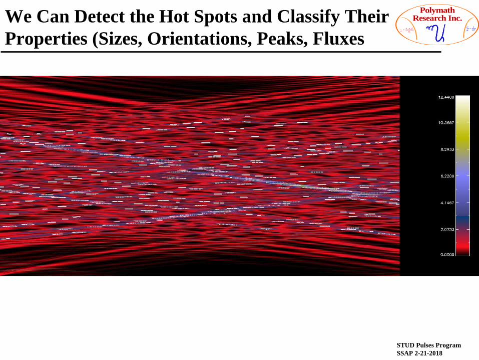
We Can Detect the Hot Spots and Classify Their Properties (Sizes, Orientations, Peaks, Fluxes

STUD Pulses ProgramSSAP 2-21-2018
PolymathResearch Inc.
pe2 = 4 ne e2
me
e2
!c≈
1137
Once You Detect the Hot Spots You Can Classify Their Properties & Find Correlations
0
2
4
6
8
10
12
14
16
0 50 100 150 200 250 300 350
Classification of Hot Spot Statistics
FwhmB
Wid
th o
f Det
ectd
Hot
Spo
t
Length of Detected Hot Spot
0
2000
4000
6000
8000
1 104
2 4 6 8 10 12
Integrated Fluxes in Each Detected Hot Spot
Flux
Flux
Peak Value

STUD Pulses ProgramSSAP 2-21-2018
PolymathResearch Inc.
pe2 = 4 ne e2
me
e2
!c≈
1137
Two Realizations of Sections of f/20 Beams
400
600
800
1000
1200
1400
1600
0 50 100 150 200 250 300
Overlap of Hot Spot Peak Locations
Y_p
eak
Loca
tion
X_peak Location
STUD Pulses ProgramSSAP 2-21-2018
PolymathResearch Inc.
pe2 = 4 ne e2
me
e2
!c≈
1137
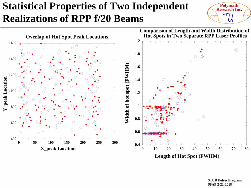
Statistical Properties of Two Independent Realizations of RPP f/20 Beams
0.4
0.6
0.8
1
1.2
1.4
1.6
1.8
2
0 10 20 30 40 50 60 70 80
Comparison of Length and Width Distribution of Hot Spots in Two Separate RPP Laser Profiles
Wid
th o
f hot
spot
(FW
HM
)
Length of Hot Spot (FWHM)
400
600
800
1000
1200
1400
1600
0 50 100 150 200 250 300
Overlap of Hot Spot Peak Locations
Y_p
eak
Loca
tion
X_peak Location
STUD Pulses ProgramSSAP 2-21-2018
PolymathResearch Inc.
pe2 = 4 ne e2
me
e2
!c≈
1137
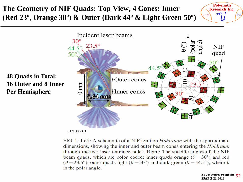
The Geometry of NIF Quads: Top View, 4 Cones: Inner (Red 23º, Orange 30º) & Outer (Dark 44º & Light Green 50º)
52
48 Quads in Total:16 Outer and 8 Inner Per Hemisphere

STUD Pulses ProgramSSAP 2-21-2018
PolymathResearch Inc.
pe2 = 4 ne e2
me
e2
!c≈
1137
SRS and SBS in the Strong Damping Limit Driven by STUD Pulses
L1 a1 = ∂∂t
+V1∂∂z
+ i β1 ∇⊥2 +ν1 −
γ 02 a0
2
ν2
⎛
⎝⎜
⎞
⎠⎟ a1 = γ 0a0e
iϕ
ν2
S 2*+S1
L0 a0 = ∂∂t
−V0∂∂z
− i β2 ∇⊥2 +ν0 −
γ 02 a1
2
ν2
⎛
⎝⎜
⎞
⎠⎟ a0 = γ 0
*a1e−iϕ
ν2
S2 + S0
ν2 = ν2 − i V2 k0 z( ) − k1 z( ) − k2 z( )#$ %&
S0 z,t; x⊥( ) = fz
z − zC , i
zW ,i
#
$%&
'(S
0, j
(i ) t − tC , j
tW , j
#
$%
&
'(
j=1
Nspikes
∑i=1
NHS
∑
Transform into a frame moving with theSTUD pulse SPIKES and do integrationover pulses as integrals over space (z).
Then average over transverse distributionswhich reflect the hot spot exponential intensity statistics.
€
∂∂t
+V1∂∂z
+ν1⎛⎝⎜
⎞⎠⎟ a1
2 = ∂∂t
−V0∂∂z
+ν0⎛⎝⎜
⎞⎠⎟ a0
2 =2 γ 0
2 a02 a1
2
v22 +V2
2 ′k2( )2⎡⎣
⎤⎦
+ 4Reγ 0 a0 a1
* S2* eiϕ v2 − iV2 ′k2( )
v22 +V2
2 ′k2( )2⎡⎣
⎤⎦
⎡
⎣
⎢⎢
⎤
⎦
⎥⎥
Action flux conservation:
STUD Pulses ProgramSSAP 2-21-2018
PolymathResearch Inc.
pe2 = 4 ne e2
me
e2
!c≈
1137
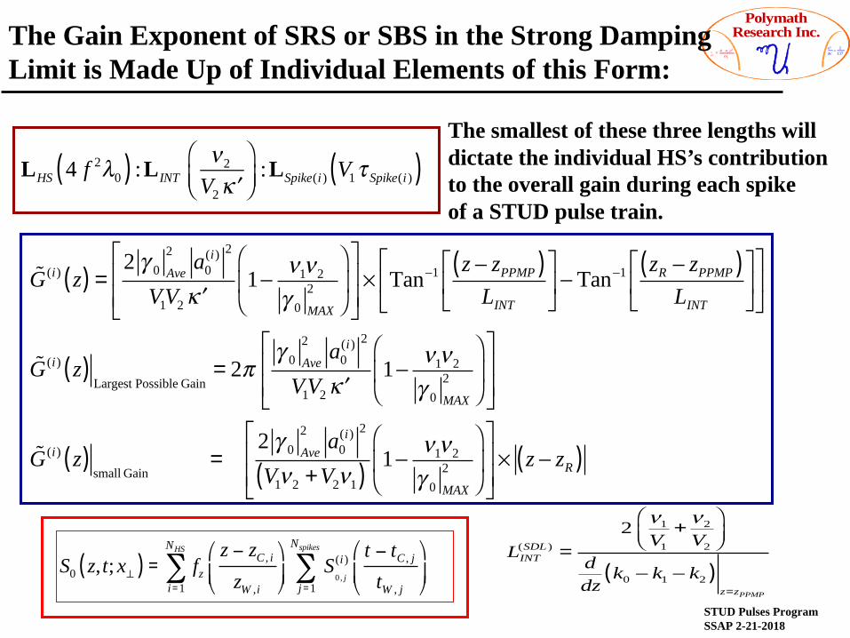
The Gain Exponent of SRS or SBS in the Strong Damping Limit is Made Up of Individual Elements of this Form:
S0 z,t; x⊥( ) = fz
z − zC , i
zW ,i
#
$%&
'(S
0, j
(i ) t − tC , j
tW , j
#
$%
&
'(
j=1
Nspikes
∑i=1
NHS
∑
LHS 4 f 2λ0( ) :LINTν2
V2 ′κ⎛⎝⎜
⎞⎠⎟
:LSpike(i ) V1τ Spike(i )( )The smallest of these three lengths will dictate the individual HS’s contribution to the overall gain during each spike of a STUD pulse train.
G(i) z( ) =2 γ 0 Ave
2 a0(i) 2
V1V2 ′κ1− ν1ν2
γ 0 MAX
2
⎛
⎝⎜
⎞
⎠⎟
⎡
⎣⎢⎢
⎤
⎦⎥⎥× Tan−1 z − zPPMP( )
LINT
⎡
⎣⎢
⎤
⎦⎥ − Tan−1 zR − zPPMP( )
LINT
⎡
⎣⎢
⎤
⎦⎥
⎡
⎣⎢
⎤
⎦⎥
G(i) z( )Largest Possible Gain
= 2πγ 0 Ave
2 a0(i) 2
V1V2 ′κ1− ν1ν2
γ 0 MAX
2
⎛
⎝⎜
⎞
⎠⎟
⎡
⎣⎢⎢
⎤
⎦⎥⎥
G(i) z( )small Gain
=2 γ 0 Ave
2 a0(i) 2
V1ν2 +V2ν1( ) 1− ν1ν2
γ 0 MAX
2
⎛
⎝⎜
⎞
⎠⎟
⎡
⎣⎢⎢
⎤
⎦⎥⎥× z − zR( )
LINT(SDL ) =
2 ν1
V1
+ ν2
V2
⎛⎝⎜
⎞⎠⎟
ddz
k0 − k1 − k2( )z=zPPMP

STUD Pulses ProgramSSAP 2-21-2018
PolymathResearch Inc.
pe2 = 4 ne e2
me
e2
!c≈
1137
Looking at the IAW on a Linear vs Log Scale for an RPP Beam @ 3 Times + the Pump
55