control of fuel cells - ntnu
TRANSCRIPT

Federico Zenith
Control of fuel cells
Doctoral thesisfor the degree of philosophiæ doctor
Trondheim, June 2007
Norwegian University of Science and TechnologyFaculty of Natural Sciences and TechnologyDepartment of Chemical Engineering

ii
NTNU
Norwegian University of Science and Technology
Doctoral thesisfor the degree of philosophiæ doctor
Faculty of Natural Sciences and TechnologyDepartment of Chemical Engineering
© 2007 Federico Zenith. Some rights reserved. This thesis is distributed according to to the terms of the Attribution-Share Alike 3.0 licence by Creative Commons. You are free to share (i.e. to copy, distribute, transmit and adapt)the work, under the conditions that you must attribute the work in the manner specified by the author (but notin any way that suggests that he endorses you or your use of the work), and that if you alter, transform, or buildupon this work, you may distribute the resulting work only under the same, similar or a compatible licence.
This thesis was typeset in Palatino and AMS Euler by the author using LATEX 2ε.
ISBN 978-82-471-1433-9 (printed version)ISBN 978-82-471-1447-6 (electronic version)ISSN 1503-8181
Doctoral theses at NTNU, 2007:65
Printed by NTNU-trykk

Abstract
This thesis deals with control of fuel cells, focusing on high-temperature proton-exchange-membrane fuel cells.
Fuel cells are devices that convert the chemical energy of hydrogen, methanol orother chemical compounds directly into electricity, without combustion or thermalcycles. They are efficient, scalable and silent devices that can provide power to awide variety of utilities, from portable electronics to vehicles, to nation-wide electricgrids.
Whereas studies about the design of fuel cell systems and the electrochemicalproperties of their components abound in the open literature, there has been only aminor interest, albeit growing, in dynamics and control of fuel cells.
In the relatively small body of available literature, there are some apparentlycontradictory statements: sometimes the slow dynamics of fuel cells is claimed topresent a control problem, whereas in other articles fuel cells are claimed to be easyto control and able to follow references that change very rapidly. These contradic-tions are mainly caused by differences in the sets of phenomena and dynamics thatthe authors decided to investigate, and also by how they formulated the controlproblem. For instance, there is little doubt that the temperature dynamics of a fuelcell can be slow, but users are not concerned with the cell’s temperature: poweroutput is a much more important measure of performance.
Fuel cells are very multidisciplinary systems, where electrical engineering, elec-trochemistry, chemical engineering and materials science are all involved at vari-ous levels; it is therefore unsurprising that few researchers can master all of thesebranches, and that most of them will neglect or misinterpret phenomena they areunfamiliar with.
The ambition of this thesis is to consider the main phenomena influencing thedynamics of fuel cells, to properly define the control problem and suggest possibleapproaches and solutions to it.
This thesis will focus on a particular type of fuel cell, a variation of proton-exchange-membrane fuel cells with a membrane of polybenzimidazole instead of
iii

iv Abstract
the usual, commercially available Nafion. The advantages of this particular typeof fuel cells for control are particularly interesting, and stem from their operationat temperatures higher than those typical of Nafion-based cells: these new cells donot have any water-management issues, can remove more heat with their exhaustgases, and have better tolerance to poisons such as carbon monoxide.
The first part of this thesis will be concerned with defining and modelling thedynamic phenomena of interest. Indeed, a common mistake is to assume that fuelcells have a single dynamics: instead, many phenomena with radically differenttime scales concur to define a fuel-cell stack’s overall behaviour. The dynamics ofinterest are those of chemical engineering (heat and mass balances), of electrochem-istry (diffusion in electrodes, electrochemical catalysis) and of electrical engineer-ing (converters, inverters and electric motors). The first part of the thesis will firstpresent some experimental results of importance for the electrochemical transient,and will then develop the equations required to model the four dynamic modeschosen to represent a fuel-cell system running on hydrogen and air at atmosphericpressure: cathodic overvoltage, hydrogen pressure in the anode, oxygen fraction inthe cathode and stack temperature.
The second part will explore some of the possible approaches to control thepower output from a fuel-cell stack. It has been attempted to produce a modu-larised set of controllers, one for each dynamics to control. It is a major point of thethesis, however, that the task of controlling a fuel cell is to be judged exclusively byits final result, that is power delivery: all other control loops, however independent,will have to be designed bearing that goal in mind.
The overvoltage, which corresponds nonlinearly to the rate of reaction, is con-trolled by operating a buck-boost DC/DC converter, which in turn is modelled andcontrolled with switching rules. Hydrogen pressure, being described by an un-stable dynamic equation, requires feedback to be controlled. A controller with PI
feedback and a feedforward part to improve performance is suggested. The oxy-gen fraction in the cathodic stream cannot be easily measured with a satisfactorybandwidth, but its dynamics is stable and disturbances can be measured quite pre-cisely: it is therefore suggested to use a feedforward controller. Contrary to the mostcommon approach for Nafion-based fuel cells, temperature is not controlled with aseparate cooling loop: instead, the air flow is used to cool the fuel-cell stack. Thissignificantly simplifies the stack design, operation and production cost. To controltemperature, it is suggested to use a P controller, possibly with a feedforward com-ponent. Simulations show that this approach to stack cooling is feasible and posesno or few additional requirements on the air flow actuator that is necessary to con-trol air composition in the cathode.

Acknowledgements
I would like to thank my supervisor, professor Sigurd Skogestad, for having offeredme the opportunity of writing this work and for his support and patience in thesefour years.
This work would not have been possible without the collaboration of severalprofessors, researchers and PhD students from the Department of Materials Tech-nology at NTNU: I would like to thank professors Reidar Tunold and Børre Børresenand researchers Ole-Edvard Kongstein and Frode Seland, who were co-authors inmy first paper, for their data, suggestions, and patience. Børre and Frode deserveadditional thanks for helping me in obtaining the experimental data presented inchapter 2.
My thanks go to Helge Weydahl, also from the Department of Materials Technol-ogy and with whom I shared my office for three years, for many fruitful discussions,in particular about the electrochemical transient.
I would like to thank Steffen Møller-Holst from SINTEF for his invaluable effortsin coordinating various projects related to hydrogen and fuel cells.
I am thankful to all the colleagues I met during my stay at the Department ofChemical Engineering for creating a great work environment.
Finally, funding from Statoil AS and the Norwegian Research Council is grate-fully acknowledged.
v

vi Acknowledgements

Contents
Abstract iii
Acknowledgements v
List of Figures xi
List of Tables xv
Notation xvii
1 Introduction 11.1 Thesis Overview . . . . . . . . . . . . . . . . . . . . . . . . . . . . . . 11.2 Motivation . . . . . . . . . . . . . . . . . . . . . . . . . . . . . . . . . . 21.3 Polybenzimidazole-Membrane Fuel Cells . . . . . . . . . . . . . . . . 3
1.3.1 Water Management in Nafion Membranes . . . . . . . . . . . 31.3.2 Advantages of Polybenzimidazole Membranes . . . . . . . . . 4
1.4 Publications . . . . . . . . . . . . . . . . . . . . . . . . . . . . . . . . . 51.4.1 Journal Articles . . . . . . . . . . . . . . . . . . . . . . . . . . . 51.4.2 Conferences and Seminars . . . . . . . . . . . . . . . . . . . . . 6
I Dynamics of Fuel Cells 9
2 Experimental Measurements 112.1 Literature Review . . . . . . . . . . . . . . . . . . . . . . . . . . . . . . 112.2 Laboratory Setup . . . . . . . . . . . . . . . . . . . . . . . . . . . . . . 12
2.2.1 Experimental Procedure . . . . . . . . . . . . . . . . . . . . . . 132.2.2 Uncertainty Analysis . . . . . . . . . . . . . . . . . . . . . . . . 14
2.3 Results and Discussion . . . . . . . . . . . . . . . . . . . . . . . . . . . 152.3.1 Polarisation Curve . . . . . . . . . . . . . . . . . . . . . . . . . 15
vii

viii Contents
2.3.2 Resistance Steps . . . . . . . . . . . . . . . . . . . . . . . . . . . 162.3.3 Effect of Flow Disturbances . . . . . . . . . . . . . . . . . . . . 18
2.4 Conclusions . . . . . . . . . . . . . . . . . . . . . . . . . . . . . . . . . 19
3 Electrochemical Modelling 233.1 Literature Review . . . . . . . . . . . . . . . . . . . . . . . . . . . . . . 233.2 Modelling Principles and Assumptions . . . . . . . . . . . . . . . . . 243.3 Diffusion . . . . . . . . . . . . . . . . . . . . . . . . . . . . . . . . . . . 26
3.3.1 The Stefan-Maxwell Equations . . . . . . . . . . . . . . . . . . 263.3.2 Simplified Diffusion . . . . . . . . . . . . . . . . . . . . . . . . 273.3.3 Distributed Layer Thickness . . . . . . . . . . . . . . . . . . . 29
3.4 Calculating the Cell Voltage . . . . . . . . . . . . . . . . . . . . . . . . 303.5 Dynamics . . . . . . . . . . . . . . . . . . . . . . . . . . . . . . . . . . 333.6 Time Constants . . . . . . . . . . . . . . . . . . . . . . . . . . . . . . . 343.7 Parameter Estimation and Simulation . . . . . . . . . . . . . . . . . . 363.8 Simulation . . . . . . . . . . . . . . . . . . . . . . . . . . . . . . . . . . 383.9 Impedance Measurements . . . . . . . . . . . . . . . . . . . . . . . . . 383.10 Instantaneous Characteristics . . . . . . . . . . . . . . . . . . . . . . . 41
3.10.1 Transient Behaviour . . . . . . . . . . . . . . . . . . . . . . . . 423.10.2 Graphical Representation of Time Constants . . . . . . . . . . 44
3.11 Perfect Control of the Electrochemical Transient . . . . . . . . . . . . 453.11.1 Implicit Limitations . . . . . . . . . . . . . . . . . . . . . . . . 46
3.12 Conclusions . . . . . . . . . . . . . . . . . . . . . . . . . . . . . . . . . 46
4 Mass and Energy Modelling 494.1 Literature Review . . . . . . . . . . . . . . . . . . . . . . . . . . . . . . 494.2 Mass Balances . . . . . . . . . . . . . . . . . . . . . . . . . . . . . . . . 51
4.2.1 Dead-End Flows . . . . . . . . . . . . . . . . . . . . . . . . . . 514.2.2 Open-End Flows . . . . . . . . . . . . . . . . . . . . . . . . . . 52
4.3 Energy Balance . . . . . . . . . . . . . . . . . . . . . . . . . . . . . . . 574.3.1 Air Cooling . . . . . . . . . . . . . . . . . . . . . . . . . . . . . 574.3.2 External Heating for Cold Start-up . . . . . . . . . . . . . . . . 584.3.3 Enthalpy-Balance Equations . . . . . . . . . . . . . . . . . . . . 58
4.4 Cell Stacks . . . . . . . . . . . . . . . . . . . . . . . . . . . . . . . . . . 60
II Control of Fuel Cells 65
5 Control Structure for Fuel Cells 67

Contents ix
5.1 Literature Review . . . . . . . . . . . . . . . . . . . . . . . . . . . . . . 675.2 Dynamic Modes of Fuel Cells . . . . . . . . . . . . . . . . . . . . . . . 715.3 Controlling the Reaction Rate . . . . . . . . . . . . . . . . . . . . . . . 72
5.3.1 Manipulating the Reactant Feed . . . . . . . . . . . . . . . . . 735.3.2 Manipulating the External Circuit . . . . . . . . . . . . . . . . 74
5.4 Controlling Reactant Concentrations . . . . . . . . . . . . . . . . . . . 755.5 Controlling Stack Temperature . . . . . . . . . . . . . . . . . . . . . . 765.6 Conclusions . . . . . . . . . . . . . . . . . . . . . . . . . . . . . . . . . 77
6 Converter Control 836.1 Choice of Converter Type . . . . . . . . . . . . . . . . . . . . . . . . . 846.2 Effects of Discontinuous Currents in the Input . . . . . . . . . . . . . 866.3 Identifying a Controlled Variable: DC Motors . . . . . . . . . . . . . . 886.4 Pulse-Width Modulation . . . . . . . . . . . . . . . . . . . . . . . . . . 91
6.4.1 Oscillation Frequency . . . . . . . . . . . . . . . . . . . . . . . 926.5 Pulse-Width Modulation: H∞ Linear Control . . . . . . . . . . . . . . 93
6.5.1 Plant Linearisation and Controllability Analysis . . . . . . . . 946.5.2 Problem Formulation . . . . . . . . . . . . . . . . . . . . . . . 95
6.6 Pulse-Width Modulation: Feedforward Control . . . . . . . . . . . . . 1016.6.1 Half-Delay Filtering . . . . . . . . . . . . . . . . . . . . . . . . 102
6.7 Pulse-Width Modulation: Input-Output Linearisation . . . . . . . . . 1046.7.1 Change of Variables . . . . . . . . . . . . . . . . . . . . . . . . 1056.7.2 Internal Dynamics . . . . . . . . . . . . . . . . . . . . . . . . . 1076.7.3 Stabilisation of the Internal Dynamics . . . . . . . . . . . . . . 1096.7.4 Feedback with Input Bounds . . . . . . . . . . . . . . . . . . . 1106.7.5 Feedforward with Internal Oscillation Dampening . . . . . . 111
6.8 Switching Rules . . . . . . . . . . . . . . . . . . . . . . . . . . . . . . . 1136.8.1 Control Rules . . . . . . . . . . . . . . . . . . . . . . . . . . . . 1146.8.2 Performance of the Switching Rules . . . . . . . . . . . . . . . 1166.8.3 Computational Performance . . . . . . . . . . . . . . . . . . . 119
6.9 Conclusions . . . . . . . . . . . . . . . . . . . . . . . . . . . . . . . . . 120
7 Composition and Temperature Control 1237.1 Power Load on the Stack . . . . . . . . . . . . . . . . . . . . . . . . . . 1247.2 Pressure Control of Dead-End Flows (Anode) . . . . . . . . . . . . . . 1267.3 Composition Control of Open-End Flows (Cathode) . . . . . . . . . . 130
7.3.1 Measurement Dynamics . . . . . . . . . . . . . . . . . . . . . . 1307.3.2 Time Constants of Composition Dynamics . . . . . . . . . . . 1317.3.3 Feedforward Control . . . . . . . . . . . . . . . . . . . . . . . . 131

x Contents
7.3.4 Dimensioning Criterion Based on Actuator Power Consumption1337.4 Temperature Control . . . . . . . . . . . . . . . . . . . . . . . . . . . . 133
7.4.1 Optimal Reference Value for Temperature Control . . . . . . . 1357.4.2 Hydrogen in the Cathodic Flow as an Input Variable . . . . . 1367.4.3 Measurement Dynamics . . . . . . . . . . . . . . . . . . . . . . 1367.4.4 Time Constants of Temperature Dynamics . . . . . . . . . . . 1377.4.5 Controller Synthesis and Simulation . . . . . . . . . . . . . . . 1377.4.6 Temperature Control with Hydrogen Combustion . . . . . . . 140
7.5 Conclusions . . . . . . . . . . . . . . . . . . . . . . . . . . . . . . . . . 1437.5.1 Dimensioning Criteria . . . . . . . . . . . . . . . . . . . . . . . 144
8 Conclusions 1478.1 Suggested Control Strategy . . . . . . . . . . . . . . . . . . . . . . . . 1488.2 Further Work . . . . . . . . . . . . . . . . . . . . . . . . . . . . . . . . 149
A Model Code 151
B H∞ Synthesis Plots 153
Index 161

List of Figures
2.1 Laboratory setup for experiments . . . . . . . . . . . . . . . . . . . . . 132.2 Experimental polarisation curve . . . . . . . . . . . . . . . . . . . . . 152.3 Experimental steps in resistance . . . . . . . . . . . . . . . . . . . . . . 162.4 One particular resistance step . . . . . . . . . . . . . . . . . . . . . . . 172.5 Voltage transients of resistance steps . . . . . . . . . . . . . . . . . . . 182.6 Transients induced by oxygen flow . . . . . . . . . . . . . . . . . . . . 19
3.1 Composition profiles through a fuel cell . . . . . . . . . . . . . . . . . 253.2 Simulated diffusion transient . . . . . . . . . . . . . . . . . . . . . . . 273.3 Ideal and real layers . . . . . . . . . . . . . . . . . . . . . . . . . . . . 293.4 Ideal and real layers . . . . . . . . . . . . . . . . . . . . . . . . . . . . 303.5 Diagram of the fuel-cell model . . . . . . . . . . . . . . . . . . . . . . 333.6 Residual plot of parametric regression . . . . . . . . . . . . . . . . . . 363.7 Simulated transient . . . . . . . . . . . . . . . . . . . . . . . . . . . . . 383.8 Simulated MOSFET transient . . . . . . . . . . . . . . . . . . . . . . . . 393.9 Impedance spectroscopy for a fuel cell . . . . . . . . . . . . . . . . . . 403.10 Polarisation curve and instantaneous characteristic . . . . . . . . . . 413.11 Phase-plane transients at current or voltage changes . . . . . . . . . . 423.12 Phase-plane transients at load changes . . . . . . . . . . . . . . . . . . 433.13 Graphical interpretation of the transient’s driving force . . . . . . . . 453.14 Power overshoot at load changes . . . . . . . . . . . . . . . . . . . . . 45
4.1 Flows in a fuel cell . . . . . . . . . . . . . . . . . . . . . . . . . . . . . 504.2 Polarisation curves when consuming oxygen . . . . . . . . . . . . . . 554.3 Maximum power outputs from a fuel cell when consuming oxygen . 554.4 Flow layout for a PBI fuel cell . . . . . . . . . . . . . . . . . . . . . . . 594.5 Air flow through fuel cells . . . . . . . . . . . . . . . . . . . . . . . . . 614.6 Flow layout for a fuel-cell stack . . . . . . . . . . . . . . . . . . . . . . 62
xi

xii List of Figures
5.1 Controlling a fuel cell with reactant flow . . . . . . . . . . . . . . . . . 685.2 Interactions of dynamics in fuel cells . . . . . . . . . . . . . . . . . . . 725.3 Linear control . . . . . . . . . . . . . . . . . . . . . . . . . . . . . . . . 755.4 Proposed control structure . . . . . . . . . . . . . . . . . . . . . . . . . 78
6.1 Definition of duty ratio . . . . . . . . . . . . . . . . . . . . . . . . . . . 846.2 Scheme of a buck converter . . . . . . . . . . . . . . . . . . . . . . . . 846.3 Scheme of a buck converter . . . . . . . . . . . . . . . . . . . . . . . . 856.4 Scheme of a buck-boost converter . . . . . . . . . . . . . . . . . . . . . 866.5 Direct connection between fuel cell and converter . . . . . . . . . . . 876.6 Insertion of a capacitance between a fuel cell and a buck-boost converter 886.7 A typical model of a DC motor . . . . . . . . . . . . . . . . . . . . . . 896.8 Cascade control layout . . . . . . . . . . . . . . . . . . . . . . . . . . . 916.9 Oscillations for constant duty ratio . . . . . . . . . . . . . . . . . . . . 926.10 Weights for H∞ synthesis . . . . . . . . . . . . . . . . . . . . . . . . . 966.11 H∞ controller for various D . . . . . . . . . . . . . . . . . . . . . . . . 986.12 H∞-controlled system for various Vin and IL . . . . . . . . . . . . . . 1006.13 Feedforward control by filtering of input D. . . . . . . . . . . . . . . . 1016.14 The half-delay input filter . . . . . . . . . . . . . . . . . . . . . . . . . 1036.15 Simulation of a series of steps with feedforward control . . . . . . . . 1036.16 Effect of disturbance with feedforward filter . . . . . . . . . . . . . . 1046.17 Values of ψ in the phase plane . . . . . . . . . . . . . . . . . . . . . . . 1066.18 Effect of unstable internal dynamics, I . . . . . . . . . . . . . . . . . . 1086.19 Effect of unstable internal dynamics, II . . . . . . . . . . . . . . . . . . 1086.20 Steps in reference with oscillation dampening . . . . . . . . . . . . . . 1126.21 Step in disturbance with oscillation dampening . . . . . . . . . . . . . 1126.22 Operating modes of a converter . . . . . . . . . . . . . . . . . . . . . . 1146.23 Switching rules . . . . . . . . . . . . . . . . . . . . . . . . . . . . . . . 1166.24 Simulink implementation of the switching rules . . . . . . . . . . . . 1176.25 Transient for switching rules . . . . . . . . . . . . . . . . . . . . . . . . 1186.26 Case of zero reference and disturbance . . . . . . . . . . . . . . . . . . 118
7.1 The New European Driving Cycle . . . . . . . . . . . . . . . . . . . . 1257.2 Effect of conversion on a cell’s power output . . . . . . . . . . . . . . 1267.3 Cell conditions during the NEDC cycle . . . . . . . . . . . . . . . . . . 1277.4 Control diagram for pure hydrogen pressure in a dead-end manifold 1287.5 Hydrogen pressure with a PI feedback controller and feedforward . . 1297.6 Oxygen fraction with a feedforward controller . . . . . . . . . . . . . 1327.7 Specific heats of main chemical species . . . . . . . . . . . . . . . . . . 135

List of Figures xiii
7.8 Performance of temperature control . . . . . . . . . . . . . . . . . . . 1397.9 Influence of composition control on temperature control . . . . . . . 1407.10 Air flow requirements of composition and temperature control . . . . 1417.11 Start-up dynamics . . . . . . . . . . . . . . . . . . . . . . . . . . . . . . 142
8.1 Time scales of the dynamic modes of fuel cells . . . . . . . . . . . . . 1488.2 The suggested layout for control of a PBI fuel cell stack . . . . . . . . 149
B.1 H∞ controller for various IL . . . . . . . . . . . . . . . . . . . . . . . . 154B.2 H∞ controller for various Vin . . . . . . . . . . . . . . . . . . . . . . . 155B.3 H∞ controller for various Vin and IL . . . . . . . . . . . . . . . . . . . 156B.4 H∞-controlled-system for various D . . . . . . . . . . . . . . . . . . . 157B.5 H∞-controlled system for various IL . . . . . . . . . . . . . . . . . . . 158B.6 H∞-controlled system for various Vin . . . . . . . . . . . . . . . . . . 159

xiv List of Figures

List of Tables
3.1 Dynamic model equations . . . . . . . . . . . . . . . . . . . . . . . . . 343.2 Results of parameter regression . . . . . . . . . . . . . . . . . . . . . . 37
7.1 Parameters for vehicle dynamics . . . . . . . . . . . . . . . . . . . . . 125
xv

xvi List of Tables

Notation
An effort has been made in this thesis to maintain unique and consistent meaningsfor most symbols. It was however decided to use the same symbol for more entitieswhen the symbol is customary in both fields and its usage does not cause misunder-standings. In particular, both voltage and volume are usually denoted by the letterV : as they can occur simultaneously in a number of equations related to fuel cells,it was chosen to represent the least common of the two, volume, using the typefaceV.
A Area [m2]a Activity [−]C Capacitance [F]Cd Drag coefficient [−]Crf Rolling friction coefficient [−]cp Molar specific heat [J/K mol]cp Areal specific heat [J/K m2]D Diffusion coefficient [m2 s]
also Duty ratio [−]E Reversible potential [V]F Faraday constant [C]f Frequency [Hz]g Gravitational acceleration [m/s2]
also Specific Gibbs free energy [J/mol]H Enthalpy [J]H Enthalpy flow [W]h Specific enthalpy [J/mol]I Current [A]i Current density [A/m2]L Inductance [H]k Reaction constant [mol/m2 s]m Mass [kg]N Molar flux [mol/m2 s]n Exchanged electrons [−]
also Number of moles [mol]n Molar flow [mol/s]P Power [W]p Pressure [Pa]
also Specific power [W/m2]R Ideal gas constant [J/mol K]
also Resistance [Ω]r Specific resistance [Ω m2]s Laplace variable [rad/s]T Period [s]
also Temperature [K]also Torque [N m]
t Time [s]V Voltage [V]V Volume [m3]v Velocity [m/s]X Conversion [−]
also Reactance [Ω]x Molar fraction [−]Z Impedance [Ω]
Greek Letters
α Symmetry factor [−]
xvii

xviii Notation
ε Porosity [−]ζ Damping factor [−]η Overvoltage [V]θ Delay [s]Λ Distributed thickness [m]λ Equivalent layer thickness [m]µ Mean [−]ν Stoichiometric coefficient [−]
ρ Density [kg/m3]also Probability density [−]
σ Standard deviation [−]τ Time constant [s]
also Tortuosity [−]Φ Magnetic flux [Wb]ω Frequency [rad/s]

Chapter 1
Introduction
1.1 Thesis Overview
This thesis is split in two main parts. The first part is on the dynamics of fuel cells,and the second one on how control can be applied.
The first part starts with some experiments pertaining the overvoltage dynam-ics of fuel cells, presented in chapter 2. Then, the following chapter interprets theresults proposing a simplified electrochemical model, which is used to obtain esti-mates of four model parameters from experimental data. The model’s structure isanalysed to obtain a theorem proving that, under general assumptions, overvoltagedynamics poses no limit to the overall dynamic performance of the fuel cell. Thecell is then studied from a process engineer’s point of view, focusing on mass andenergy balances. The effects of different cell-stacking configurations is also brieflyconsidered.
The second part begins with chapter 5, in which an overall control strategy forfuel cells is outlined, selecting which control variables are suitable for the variouscontrol loops. The actual implementation of control strategies is presented in thetwo following chapters: chapter 6 considers the design of a controller for a DC/DC
converter, whereas chapter 7 presents the control solutions for mass and energybalances.
The software written for this thesis is attached to the PDF version of this the-sis, or can be obtained contacting the author. The terms of usage and installationinstructions are given in appendix A.
1

2 Introduction
1.2 Motivation
Fuel cells are devices that produce electric power by direct conversion of a fuel’schemical energy. They are being extensively studied in many research environmentsfor the possibility they offer of converting energy without the losses associated withthermal cycles, thereby having the potential to increase efficiency. Compared toother power sources, they operate silently, have no major moving parts, can be as-sembled easily into larger stacks, and (when run on hydrogen) produce only wateras a by-product.
Fuel cells are essentially energy converters. Fuel cells resemble batteries in manyways, but in contrast to them they do not store the chemical energy: fuel has to becontinuously provided to the cell to maintain the power output.
Various designs for fuel cells have been proposed, the most popular being theproton-exchange-membrane fuel cell (PEM) (usually with a Nafion membrane), op-erating at temperatures up to about 100 °C, and the solid-oxide fuel cell (SOFC), op-erating at temperatures of about 800 °C or higher. Whereas the underlying principleis always to extract electricity without combustion, each design presents differentproblems and advantages, and has unique characteristics that make it more appro-priate for different environments.
Fuel cells of various kinds have been proposed for many power-productiontasks, ranging from pacemakers to power plants, but their adoption is still in itsinfancy. Most fuel cells are in research laboratories or in proof-of-concept appli-cations, and no product powered by fuel cells has become commonplace on themarket.
Possibly because of this focus on laboratory research, there has until recently notbeen much focus on control strategies for fuel cells. Because of the multidisciplinar-ity of the field, it has been common to investigate the control problem from oneparticular point of view, a common one being manipulating the gas flows enteringthe cell to control the power output. An objective of this thesis is to integrate pre-vious work from different areas with new insights, in order to acquire a completeview of the control issues of fuel-cell systems.
A characteristic trait of fuel-cell research is how many fields it can involve. Thereactions at the basis of its operation are the domain of electrochemistry, whereasthe energy and mass balances implied in continuously feeding reactants to the cellbelong to chemical engineering, which can also be involved in the pre-treating ofreactants. Converting the cell’s power output to the appropriate current and volt-age requires the skills of electrical engineering. Applying control theory to such amultidisciplinary system is a challenging task.

1.3. Polybenzimidazole-Membrane Fuel Cells 3
1.3 Polybenzimidazole-Membrane Fuel Cells
More and more new types of fuel cells are appearing in the open literature. Whereasthe most commonly researched are the Nafion-based PEM and solid-oxide fuel cells,many other types are being considered: some are older types that still present inter-esting aspects for researchers, such as the alkaline and molten-carbonate fuel cells,while others are entirely new concepts (such as microbial [1], formic-acid [2], and di-rect borohydride fuel cells [3]), or improvements of existing ones in various aspects,such as new electrolytes or catalysts for existing fuel cells.
This thesis does not intend to present control methods for all the currently stud-ied designs: one-size-fits-all algorithms are unlikely to exist, given the large diver-sity in the characteristics of the various types of fuel cells. A particular type of fuelcell will therefore be selected.
In choosing the fuel cell to model in this thesis, various aspects have been con-sidered. It was decided at an early stage that it should be a PEM cell, as these areamong the best studied (also within the small body of fuel-cell control literature),and most comparable models in the literature deal with these. However, PEM cellswhose membranes are Nafion-based, which is the case in the majority of publica-tions, present a serious issue for control: water management. It was therefore de-cided to study another kind of PEM, but before discussing this we will illustrate theshortcomings of Nafion membranes from the point of view of the control engineer.
1.3.1 Water Management in Nafion Membranes
Nafion membranes rely on liquid water to conduct protons through the membrane,but water content varies during operation as a consequence of reaction and evapo-ration. Too low water content will compromise the conductivity of the membrane,whereas too much water will flood the cathode and block the reaction. As a result,the acceptable target window of cell temperature versus relative humidity in thecathode gas is uncomfortably small [4, 5]. Since cells are usually electrically con-nected in series to form stacks, the failure of a single cell to carry the stack currentwill have a disrupting effect on the whole stack: the more the cells in a stack, thelarger the likelihood that such a failure will happen. In addition, the failing cellwill still be subject to the current the rest of the stack is pushing through it, caus-ing reverse electrolysis that may rapidly ruin the catalyst and force the cell to bereplaced.
In practical applications, water management is dealt with by humidifying thegas flows entering the stack and forcing the cathode gas flow to pass all cathodicsides in series, to mechanically remove any liquid water: this is however feasible

4 Introduction
only in very small stacks, as already noticed by Litz and Kordesch [6] in 1965: withmany cells, the pressure drop rapidly increases to very high levels, with increasingcosts and loss of efficiency of the fuel-cell system (Corbo et al. [7] claim that theenergetic cost of the air compressor is by far the largest one among ancillary units).However, operating all cells in parallel, with all cells connected to the same enteringand exiting manifolds, may block some cells where flooding is occurring: as thegases will take the path of least resistance, these cells will remain flooded. Again,because of the usual electrical series connections, flooding of a single cell can blockthe whole stack’s current.
Any approach to manage a membrane’s water content based on feedback controlsuffers from the fundamental problem that the liquid water content in each cell isdifficult to measure: both dry-out and flooding will result in a drop in voltage.Schumacher et al. [5] suggested inferring flooding from drops in voltage, and dry-out from variations in a cell’s impedance at 1 kHz. However, even being able tomeasure the water content, it is not obvious what should be done in case a cell isdry while another is flooded at the same time1: it would be necessary to add newmanipulated variables, such as flow-regulating valves for each cell, and devise acomplex control system.
1.3.2 Advantages of Polybenzimidazole Membranes
The newer polybenzimidazole membranes (PBI) offer an alternative to Nafion, withdifferent opportunities and challenges. They do not rely on liquid water to transportprotons through the membrane, but (in most cases) on phosphoric-acid doping [8, 9,10, 11, 12, 13], which increases their conductivity from about 10−12 S/cm [14, 15] to6.8× 10−2 S/cm. Phosphoric-acid doped PBI fuel cells can function at temperaturesas high as 200 °C [12].
Not relying on liquid water, PBI cells can operate well beyond 100 °C withoutany need for pressurisation: this generates a number of very interesting properties,in particular from the point of view of controllability [16]:
• As the phosphoric acid concentration does not change significantly over time2,membrane conductivity is more predictable and reliable.
1This could easily happen if an entering air flow, passing through all the cells in series, were notpre-humidified and sufficiently turbulent: the first cells could dry out, whereas the last ones wouldbe saturated with the vapour produced by the previous ones.
2In laboratory experiments, the anode gas is usually bubbled through H3PO4 before entering thecell to make up for any losses.

1.4. Publications 5
• Since water is produced in vapour form, cathode flooding cannot occur. It isalso much easier to model diffusion with the Stefan-Maxwell equations, as alldiffusing species are in gas phase: modelling the mass transport in Nafion fuelcells implies the difficulty of dealing with a separate liquid phase in a porousmaterial.
• High temperatures increase anodic tolerance to poisons such as CO. CO is acommon poison in hydrogen obtained by reforming, and must be kept below10 ppm in Nafion-membrane fuel cells. At the higher temperatures made at-tainable by PBI membranes, tolerance was measured to be 3 % in hydrogen atcurrent densities up to 0.8 A/cm2 at 200 °C [17]. Since this reduces the purityconstraint on the anode gas, there is no need for complex purification systemsfor reformate gases, their control loops and the losses in dynamic performancethey would introduce.
• The higher temperatures of exhaust gases allow better stack cooling, sinceoff-gases remove more heat. It could be possible to discard the separate andexpensive cooling system that Nafion-based fuel cells require.
On the other hand, PBI membranes are a more recent technology than Nafion,and hence less material is available in the literature about their properties. PBI isnot readily commercially available as Nafion is, and membranes have often to beprepared in-house, impairing the reproducibility of its properties.
Because PBI membranes have much better controllability properties comparedto Nafion-based ones, it was decided that this thesis would concentrate on this typeof fuel cells.
1.4 Publications
1.4.1 Journal Articles
• Federico Zenith and Sigurd Skogestad, Control of fuel-cell power output, Journalof Process Control 17 (2007) 333–347. Contains the proof of theorem 3.11.1about perfect control of fuel cells, and the theory outlined in section 6.8 aboutcontrol of DC/DC converters with switching rules.
• Federico Zenith, Frode Seland, Ole Edvard Kongstein, Børre Børresen, ReidarTunold and Sigurd Skogestad, Control-oriented modelling and experimental studyof the transient response of a high-temperature polymer fuel cell, Journal of PowerSources 162 (2006) 215–227. Presents the experimental data of chapter 2 and

6 Introduction
most of the analysis of chapter 3, introducing the concept of instantaneouscharacteristic.
1.4.2 Conferences and Seminars
• Federico Zenith, Control of Fuel Cells, lecture at the Institute of Energy Tech-nology of Aalborg University, December 13, 2006. It treats, albeit superficially,all chapters up to chapter 6.
• Control of fuel cells—Power control with pulse-width modulation, presentation atthe Nordic Hydrogen Seminar 2006 in Oslo, Norway, February 7, 2006. Essen-tially the same as the presentation in Denmark on January 27, but delivered toa hydrogen-oriented audience rather than a control-oriented one.
• Control of fuel cells connected to DC/DC converters, presentation delivered at the2006 Nordic Process Control Workshop in Lyngby, Denmark, January 27, 2006.Control of buck-boost converters by pulse-width modulation: half-delay feed-forward technique.
• Control of a fuel-cell powered DC vehicle motor, paper and presentation deliveredat the AIChE 2005 Annual meeting, November 2, 2005, in Cincinnati, OH,USA. Modelling and control of buck-boost converters by means of switchingrules. Applications to cascade control of DC motors.
• Dynamics and control of polybenzimidazole fuel cells, paper and presentation heldat the ECOS 2005 conference in Trondheim, Norway. Analysis of possible ma-nipulated variables (air flow, rheostats, DC/DC converters). Simulation of im-pedance measurements for parameter estimation.
• Dynamic modelling for control of fuel cells, paper and presentation delivered atthe AIChE 2004 Annual meeting, November 10, 2004, in Austin, TX, USA.Analytic expression of the time constants through an overvoltage transient,first presentation of the theorem of perfect control for overvoltage dynamics.
• Modelling and control of fuel cells, presentation delivered at the 12th Nordic Pro-cess Control Workshop, August 19, 2004, in Gothenburg, Sweden. Descriptionof PBI fuel cells in a control perspective and presentation of laboratory results.
• Modelling and experimental study of the transient response of fuel cells, poster pre-sented at the 9th Ulm Electrochemical Talks, May 17–18, 2004, in Neu-Ulm,

Bibliography 7
Germany. Presents an initial modelling of the transient in overvoltage causedby a step in the external circuit’s resistance.
Bibliography
[1] Frank Davis and Séamus P. J. Higson. Biofuel cells—recent advances and applications.Biosensors & Bioelectronics, 22:1224–1235, 2007.
[2] S. Ha, Z. Dunbar, and R. I. Masel. Characterization of a high performing passive directformic acid fuel cell. Journal of Power Sources, 158:129–136, 2006.
[3] George H. Miley, Nie Luo, Joseph Mather, Rodney Burton, Glenn Hawkins, LifengGu, Ethan Byrd, Richard Gimlin, Prajakti Joshi Shrestha, Gabriel Benavides, JuliaLaystrom, and David Carrol. Direct nabh4/h2o2 fuel cells. Journal of Power Sources,165:509–516, 2007.
[4] James Larminie and Andrew Dicks. Fuel Cell Systems Explained. Wiley, 1st edition, 1999.
[5] J. O. Schumacher, P. Gemmar, M. Denne, M. Zedda, and M. Stueber. Control of minia-ture proton exchange membrane fuel cells based on fuzzy logic. Journal of PowerSources, 129:143–151, 2004.
[6] Lawrence M. Litz and Karl V. Kordesch. Technology of hydrogen-oxygen carbon elec-trode fuel cells. In George J. Young and Henry R. Linden, editors, Fuel Cell Systems,volume 47 of Advances in chemistry, pages 166–187. American Chemical Society, 1965.
[7] P. Corbo, F. E. Corcione, F. Migliardini, and O. Veneri. Experimental assessment ofenergy-management strategies in fuel-cell propulsion systems. Journal of Power Sources,157:799–808, 2006.
[8] J. S. Wainright, J.-T. Wang, D. Weng, R. F. Savinell, and M. Litt. Acid-doped polyben-zimidazoles: A new polymer electrolyte. Journal of the Electrochemical Society, 142(7):L121–L123, July 1995.
[9] R. Bouchet, R. Miller, M. Duclot, and J. L. Souquet. A thermodynamic approach toproton conductivity in acid-doped polybenzimidazole. Solid State Ionics, 145:69–78,2001.
[10] Hongting Pu, Wolfgang H. Meyer, and Gerhard Wegner. Proton transport in polyben-zimidazole with H3PO4 or H2SO4. Journal of Polymer Science, 40(7):663–669, 2002.
[11] Alex Schechter and Robert F. Savinell. Imidazole and 1-methyl imidazole in phos-phoric acid doped polybenzimidazole electrolyte for fuel cells. Solid State Ionics, 147:181–187, 2002.

8 Introduction
[12] Ronghuan He, Qinfeng Li, Gang Xiao, and Niels J. Bjerrum. Proton conductivity ofphosphoric acid doped polybenzimidazole and its composites with inorganic protonconductors. Journal of Membrane Science, 226:169–184, 2003.
[13] Y.-L. Ma, J. S. Wainright, M. H. Litt, and R. F. Savinell. Conductivity of PBI membranesfor high-temperature polymer electrolyte fuel cells. Journal of the Electrochemical Society,151(1):A8–A16, 2004.
[14] Shaul M. Aharoni and Anthony J. Signorelli. Electrical resistivity and ESCA studieson neutral poly(alkylbenzimidazoles), their salts, and complexes. Journal of AppliedPolymer Science, 23:2653–2660, 1979.
[15] Herbert A. Pohl and Richard P. Chartoff. Carriers and unpaired spins in some organicsemiconductors. Journal of Polymer Science A, 2:2787–2806, 1964.
[16] Jianlu Zhang, Zhong Xie, Jiujun Zhang, Yanghua Tang, Chaojie Song, Titichai Na-vessin, Zhiqing Shi, Datong Song, Haijiang Wang, David P. Wilkinson, Zhong-ShengLiu, and Steven Holdcroft. High temperature PEM fuel cells. Journal of Power Sources,160:872–891, 2006.
[17] Qinfeng Li, Ronghuan He, Ji-An Gao, Jens Oluf Jensen, and Niels J. Bjerrum. TheCO poisoning effect in PEMFCs operation at temperatures up to 200 °C. Journal of theElectrochemical Society, 150(12):A1599–A1605, 2003.

Part I
Dynamics of Fuel Cells
9


Chapter 2
Experimental Measurements
In order to study the response of a polybenzimidazole fuel cell to variable resistiveloads, experiments were carried out on a PBI membrane-electrode assembly, pre-pared in-house at Department of Materials Technology of NTNU. The experimentsfocused on the electrochemical properties of the cell, and care was taken to avoidinterference from temperature transients and reactant depletion.
2.1 Literature Review
One of the first investigations of the dynamic properties of low-temperature PEM
fuel cells was published by Argyropoulos et al. [1, 2], who applied a series of cur-rents through a direct methanol fuel cell. They noted how transients in voltage werequick and often overshot their steady-state value, yielding transient operation thatwas actually better than at steady state.
A series of tests on the effect of a manipulated reactant input for direct-methanolfuel cells was conducted by Sundmacher et al. [3], which highlighted the delay be-tween reactant shut-off and its effect on cell voltage, in the range of 200 s. The au-thors assumed that current could be determined independently.
Johansen [4] studied the dynamics and control of a fuel cell with a polybenzim-idazole membrane, using a transistor load. When changing the transistor load, henoted that transients in voltage were in the order of milliseconds. When using reac-tant feed instead, response would be quick only when increasing feed, and wouldbe much slower when decreasing it.
Weydahl et al. [5] studied, in a similar fashion, the transients of alkaline fuelcells, this time with a resistive load, whose resistance was stepped between variousvalues, identifying a characteristic path in the voltage-current plot. Weydahl’s PhD
11

12 Experimental Measurements
thesis [6] contains many other experimental measurements of the dynamics of bothalkaline and PEM fuel cells under various conditions, with variable resistive loads,currents, gas flows and compositions.
Kallo et al. [7] performed a series of dynamic tests on a direct methanol fuel cell,identifying three main factors in the dynamic response: the charge double layer’scapacitance, catalyst poisoning and reactant crossover.
It has been shown by Rao and Rengaswamy [8] that current does not changestepwise during specific transients, such as when changing the external resistance,but instead follows a certain pattern, which may be described as a step change fol-lowed by what appears to be an exponential relaxation.
Benziger et al. [9] investigated the behaviour of fuel cells with a slowly changingexternal resistance. Using a Nafion membrane, they noticed how the output voltagewould rapidly change when passing a certain threshold value in the applied exter-nal resistance, in a way similar to the ignited state of CSTR reactors. They concludedthat this discontinuity was due to the water balance, as an increased water contentwould swell the membrane and improve contact with the catalyst layer. Their stud-ies concerned the time range of 103 to 104 seconds, which is far beyond the timerange of transients in overvoltage.
The effect of a large number of parameters on a PEM fuel cell’s performance wasstudied by Yan et al. [10], who concluded that the most influential parameters wereinlet humidities and temperature.
2.2 Laboratory Setup
The laboratory setup is sketched in figure 2.1. The load was a variable-resistanceboard, implemented with two resistances in parallel; in series with one of theseresistances, a switch could be opened and closed manually, changing the total resis-tance of the circuit. The value of the resistances could be selected manually from the11 positions of two corresponding knobs. The resistance board had been previouslydeveloped by Helge Weydahl in a related study [5].
The cell could be kept at a given temperature by a custom-made external electricheater with a feedback control loop, consisting of a thermocouple and an electroniccontrol unit (West 6400 1/16 DIN profile controller). It should be noted that, whereasthe laboratory setup needed make-up heat because of its small size, an applicationwill probably need cooling instead, since the reaction heat will be sufficient to main-tain its temperature.
The fuel cell, with a membrane area of 2× 2 cm2, ran on 99.5 % hydrogen and99.5 % oxygen, both at atmospheric pressure. Oxygen was fed to the cell directly,

2.2. Laboratory Setup 13
Figure 2.1: The laboratory setup for the experiments. Resistances R1 and R2 can beset to 11 different values each. The fuel cell’s voltage is measured by voltmeter V1
and passed to the data-acquisition unit. Resistance Rref, known and fixed, is used tomeasure the current; its voltage is measured by V2.
whereas hydrogen was bubbled through a 37.5 % H3PO4 solution, in order to makeup for any loss of phosphoric acid in the cell’s membrane. Both exhaust streamswere bubbled through distilled water, to provide a simple visual feedback. Allstreams were controlled with a flow-control unit by Hi-Tek.
To acquire data, an Agilent 34970A data-acquisition unit was used; the data waslater exported from its interface program to produce plots.
A polarisation curve for the cell was measured using a Wenking HP 96-20 poten-tiostat, whose voltage was set by a Wenking MVS 98 Scan Generator. When measur-ing the polarisation curve, the potentiostat substituted the resistance board in figure2.1.
2.2.1 Experimental Procedure
Some general conditions were maintained in all tests:
• The cell was kept at a constant temperature of 150 °C;
• The oxygen flow was kept at 3.7 cm3/s;
• The hydrogen flow was kept at 5.8 cm3/s.

14 Experimental Measurements
Since the data acquisition unit could only make voltage measurements, the cur-rent passing through the circuit was always calculated from the voltage over aknown, small resistance, integrated in the resistance board. The voltages measuredby the data-acquisition unit and the times at which they were taken were the onlymeasurement recorded. In order to have synchronous data for current and voltage,the time vectors associated with current and voltage outputs were merged; each ofthe outputs was then linearly interpolated on the merged time vector.
For variable-resistance tests, the fuel cell was connected to the resistance board.After having reached steady state in cell temperature and voltage, the data acquisi-tion unit was turned on and the board’s switch was flipped. For consecutive tests,the switch could be flipped again after reaching a steady state in voltage. The datacould then be saved as a comma-separated value file. To obtain maximum detail,the data-acquisition unit was set to record data as fast as possible (about every 0.1seconds).
To obtain a polarisation curve, the fuel cell was connected to the potentiostatinstead of the resistance board. Because of the slow secondary dynamics, the mea-surement took about 18 hours: the potentiostat cycled between 0.825 and 0 V at asweep rate of 25 µV/s. In order to obtain a manageable number of data points, thedata-acquisition unit was set to record data every 10 seconds.
The MEA was prepared as described in Seland et al. [11], and it was tested ina commercially available fuel cell (ElectroChem, Inc.) with one reference electrodeprobe, double serpentine flow field, originally designed for low-temperature PEM
fuel cells.
2.2.2 Uncertainty Analysis
The preparation of the membrane-electrode assembly is likely to have a major im-pact on the fuel cell’s properties. Since PBI membranes are not commercially avail-able in standard form, the variability encountered in reproducing the membranemay impair the reproducibility of the measurements reported in this thesis.
The influence of oxygen flow might depend on the number and shape of thecathode channels. Precision in hydrogen flow, instead, has been found to be oflittle consequence. The performance of the flow controllers and of the temperaturecontroller will also influence the resulting data, but this will result in systematicerror rather than uncertainty.
The precision with which the board’s resistances are known is going to have adirect influence the reliability of the measurements of current. Any unaccountednonlinearities would also disturb the measurements.

2.3. Results and Discussion 15
0
0.1
0.2
0.3
0.4
0.5
0.6
0.7
0.8
0.9
0 0.2 0.4 0.6 0.8 1 1.2 0
0.05
0.1
0.15
0.2
0.25
0.3
Vo
ltag
e, V
Po
wer
den
sity
, W/
cm2
Current density, A/cm2
VoltagePower density
Figure 2.2: Experimental polarisation curve of a PBI fuel cell at 150 °C, measuredwith a sweep rate of 25 µV/s. The arrows indicate the direction of the hysteresiscycle.
Some transients had time constants in the same order of magnitude or evenfaster than the sampling rate. It is possible that some important points might bemissed if a fast transient is not sampled with a sufficiently fast sensor, resulting in asignificantly different shape of the measured transient.
2.3 Results and Discussion
2.3.1 Polarisation Curve
The polarisation curve obtained at the conditions described in the previous sectionis shown in figure 2.2. It presents a fairly large hysteresis, a behaviour previouslyobserved in other experiments on similarPBI cells [12].
Liu et al. [12] showed that the cathodic reaction is first-order with respect to theconcentration of H+ ions, which depends on the partial pressure of water vapour:it might then be tempting to blame the hysteresis on the lag in water formation.However, given how slowly the polarisation curve was sampled, this is unlikely tobe the only reason. Likewise, temperature transients, caused by the varying poweroutput, should not have influenced such a slow sampling. Other possible causes in-clude changes in the access of oxygen to the reaction sites or changes in the catalystduring the cycle.

16 Experimental Measurements
0
0.2
0.4
0.6
0.8
1
0 0.05 0.1 0.15 0.2 0.25 0.3
Vo
ltag
e, V
Current, A
82.25 Ω 12.88 Ω5.47 Ω
2.85 Ω
Polarisation curve
Transient paths
Resistances
Figure 2.3: Path of experimental operating points in the V-I diagram after stepchanges in the external circuit’s resistance, starting from 82.25 Ω and then switchingback. The arrows indicate the path in the V-I plane, and the markers are spaced byabout 0.06 s.
2.3.2 Resistance Steps
The results obtained by switching from an initial resistance to a smaller one andback are shown in figures 2.3 and 2.4. It can be seen how the operating point movesfrom one resistance’s characteristic to the other along almost parallel, straight lines.The reason why the lines are not exactly parallel might be that sampling is not con-tinuous, and the operating point might have moved from the initial point on thenew resistance characteristic by the time a new sample is measured.
As a reference, the polarisation curve is plotted as well. The last transient is notexactly on the expected characteristic of its external resistance, most likely due toimprecision in the calculation of the resistance value.
It is clear that some transients are faster than others in the descent to steady-state; this can be seen by the number of markers, roughly spaced by 0.06 seconds,on the trajectories in the V-I plane. It appears that the electrochemical transient wasfaster the lower the resistance.
Zooming in on a specific transient provides further information. In figure 2.4the second transient, the one to 5.47 Ω, is represented in the V-I plane; the markson the line represent the sampling points. It can easily be seen that the descent tosteady state on the characteristic of the 5.47 Ω resistance was faster than the ascentto steady state on the 82.25 Ω one, when the switch on the resistance board was

2.3. Results and Discussion 17
0.6
0.65
0.7
0.75
0.8
0.85
0 0.02 0.04 0.06 0.08 0.1 0.12 0.14
Vo
ltag
e, V
Current, A
82.25 Ω
5.47 Ω
Polarisation curveTransient path
Resistances
Figure 2.4: Zoom on an experimental transient path for a step change in the externalresistance. Some drift is visible around the steady states. The markers are spacedby about 0.06 s.
turned back off.There is an indication, in other words, that the electrochemical transient can
exhibit different time constants depending on both the start and the end point. Thisbehaviour could be related to the phenomenon observed by Johansen [4], where thesame proportional controller performed too aggressively in some operating ranges,and too mildly in others.
The values assumed by the voltage are plotted versus time in figure 2.5. Theexperiments are the same as in figure 2.3. It can be seen that, after a transient in theorder of magnitude of one second, a slower transient of generally smaller amplitudeappears.
Wang and Wang [13] measured a similar behaviour for a low-temperature PEM
fuel cell, which had also been described by Ceraolo et al. [14]. In both cases, theauthors noted that slow transients in proton concentration are the cause of thesetransients. Since protons in the amorphous H3PO4 phase are important in PBI fuelcells too [12], the mechanism could be similar in principle. Compared to Wang andWang’s measurements, transients in PBI fuel cells appear to be slower.
It can be seen from figures 2.3 and 2.5 that all the transients to lower values of re-sistance seem to reach first the lower branch of the polarisation curve, to rise againto the upper one as proton concentration increases. However, the transients backto the initial, larger resistance are much larger than the gap between the branches
18 Experimental Measurements
0.64
0.66
0.68
0.7
0.72
0.74
0.76
0.78
0.8
0.82
0.84
0.86
0 20 40 60 80 100 120 140 160 180
Vo
ltag
e, V
Time, s
To 2.8548 Ω
To 5.4714 Ω
To 12.882 Ω
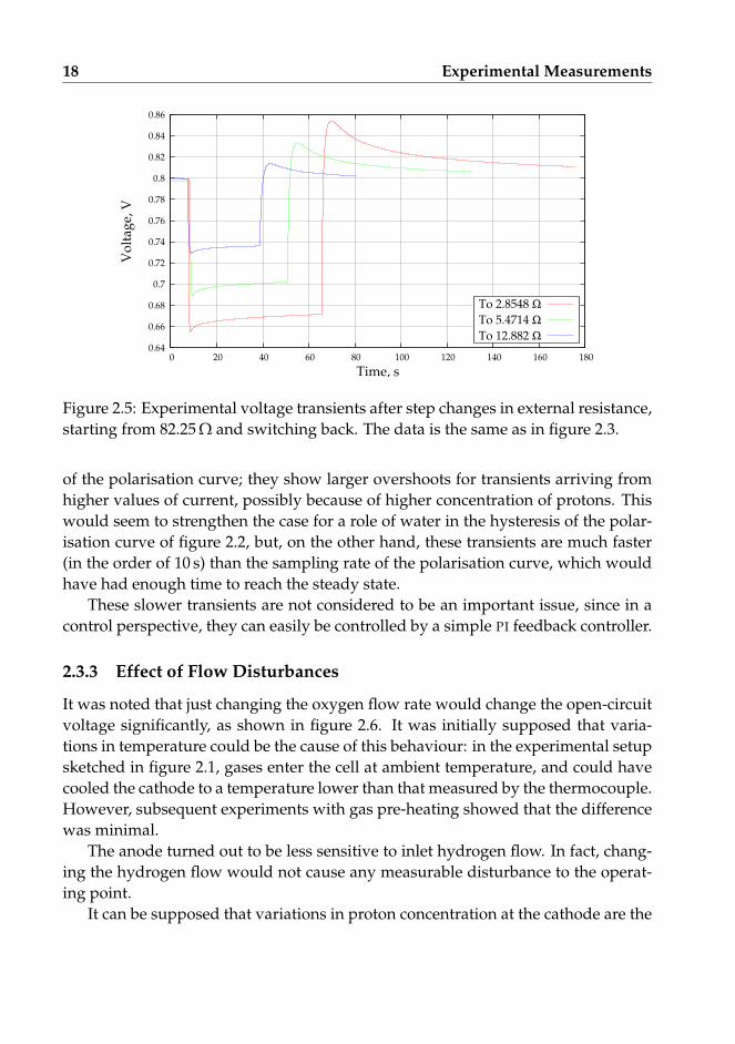
Figure 2.5: Experimental voltage transients after step changes in external resistance,starting from 82.25 Ω and switching back. The data is the same as in figure 2.3.
of the polarisation curve; they show larger overshoots for transients arriving fromhigher values of current, possibly because of higher concentration of protons. Thiswould seem to strengthen the case for a role of water in the hysteresis of the polar-isation curve of figure 2.2, but, on the other hand, these transients are much faster(in the order of 10 s) than the sampling rate of the polarisation curve, which wouldhave had enough time to reach the steady state.
These slower transients are not considered to be an important issue, since in acontrol perspective, they can easily be controlled by a simple PI feedback controller.
2.3.3 Effect of Flow Disturbances
It was noted that just changing the oxygen flow rate would change the open-circuitvoltage significantly, as shown in figure 2.6. It was initially supposed that varia-tions in temperature could be the cause of this behaviour: in the experimental setupsketched in figure 2.1, gases enter the cell at ambient temperature, and could havecooled the cathode to a temperature lower than that measured by the thermocouple.However, subsequent experiments with gas pre-heating showed that the differencewas minimal.
The anode turned out to be less sensitive to inlet hydrogen flow. In fact, chang-ing the hydrogen flow would not cause any measurable disturbance to the operat-ing point.
It can be supposed that variations in proton concentration at the cathode are the

2.4. Conclusions 19
0.74
0.76
0.78
0.8
0.82
0.84
0.86
0.88
0.9
0 500 1000 1500 2000 2500 3000 3500 4000 4500
Vo
ltag
e, V
Time, s
Figure 2.6: Experimental measure of the effect of a step in oxygen flow from 3.7 to18 cm3/s at 150 °C on open-circuit voltage. The initial step occurs when oxygen flowis started at the beginning of the experiment. The second step, at about t = 2200 s,occurs when oxygen flow is stepped up; the last step, at about t = 3600 s, whenoxygen flow is stepped back down.
cause of these transients too. When oxygen flow is increased, there is an immediateincrease in voltage due to higher oxygen partial pressure, and a subsequent decreasedue to reduction in proton concentration, caused by the reduced water partial pres-sure at the reaction site1. Conversely, when oxygen flow is reduced, there is a sharpreduction in voltage due to lower oxygen partial pressure, followed by a recoveryof proton concentration, faster than the previous transient.
This asymmetry in the dynamics of proton concentration has already been notedby Ceraolo et al. [14].
2.4 Conclusions
A laboratory setup to gather data about the transient behaviour of PBI fuel cells hasbeen presented. Data has been gathered about the steady-state polarisation curvewith a very slow scan, and transients have been studied by stepping the value ofthe resistance connected to the fuel cell: this has highlighted a particular pattern.
1Even if we are at open circuit, crossover current is causing some reaction to take place, and somewater to be formed.

20 Experimental Measurements
Some other transients, slower than the ones just mentioned, have also been ob-served. Whereas their nature is not clear, their importance is argued to be limitedfor control, as their slow development can easily be compensated for by a feedbackloop.
Bibliography
[1] P. Argyropoulos, K. Scott, and W. M. Taama. Dynamic response of the direct methanolfuel cell under variable load conditions. Journal of Power Sources, 87:153–161, 2000.
[2] P. Argyropoulos, K. Scott, and W. M. Taama. The effect of operating conditions on thedynamic response of the direct methanol fuel cell. Electrochimica Acta, 45:1983–1998,2000.
[3] K. Sundmacher, T. Schultz, S. Zhou, K. Scott, M. Ginkel, and E. D. Gilles. Dynamics ofthe direct methanol fuel cell (DMFC): experiments and model-based analysis. ChemicalEngineering Science, 56:333–341, 2001.
[4] Rune L. Johansen. Fuel cells in vehicles. Master’s thesis, Norwegian University ofScience and Technology, 2003.
[5] Helge Weydahl, Steffen Møller-Holst, Trygve Burchardt, and Georg Hagen. Dynamicbehaviour of an alkaline fuel cell – results from introductory experiments. In 1st Euro-pean Hydrogen Energy Conference, Grenoble, September 2003. CP4/123.
[6] Helge Weydahl. Dynamic behaviour of fuel cells. PhD thesis, Norwegian University ofScience and Technology, Trondheim, August 2006.
[7] Josef Kallo, Jim Kamara, Werner Lehnert, and Rittmar von Helmolt. Cell voltage tran-sients of a gas-fed direct methanol fuel cell. Journal of Power Sources, 127:181–186, 2004.
[8] R. Madhusudana Rao and Raghunathan Rengaswamy. Study of dynamic interactionsof various phenomena in proton exchange membrane fuel cells (pemfc) using detailedmodels for multivariable control. In AIChE Annual Meeting, 2005.
[9] Jay Benziger, E. Chia, J. F. Moxley, and I.G. Kevrekidis. The dynamic response of PEMfuel cells to changes in load. Chemical Engineering Science, 60:1743–1759, 2005.
[10] Qiangu Yan, Hossein Toghiani, and Heath Causey. Steady state and dynamic perfor-mance of proton exchange membrane fuel cells (PEMFCs) under various operatingconditions and load changes. Journal of Power Sources, 161(1):492–502, 2006.
[11] Frode Seland, Torstein Berning, Børre Børresen, and Reidar Tunold. Improving theperformance of high-temperature PEM fuel cells based on PBI electrolyte. Journal ofPower Sources, 160(1):27–36, 2006.

Bibliography 21
[12] Zhenyu Liu, Jesse S. Wainright, Morton H. Litt, and Robert F. Savinell. Study of theoxygen reduction reaction (ORR) at Pt interfaced with phosphoric acid doped poly-benzimidazole at elevated temperature and low relative humidity. Electrochimica Acta,51:3914–3923, 2005.
[13] Yun Wang and Chao-Yang Wang. Transient analysis of polymer electrolyte fuel cells.Eletrochimica Acta, 50:1307–1315, 2005.
[14] M. Ceraolo, C. Miulli, and A. Pozio. Modelling static and dynamic behaviour of protonexchange membrane fuel cells on the basis of electro-chemical description. Journal ofPower Sources, 113:131–144, 2003.

22 Experimental Measurements

Chapter 3
Electrochemical Modelling
This chapter will present a model of the essential electrochemical dynamics of PBI
fuel cells. The electrochemical reaction is the purpose of the cell, and it is necessaryto understand it to estimate what control performance we can expect from a fuel-cellstack.
To limit the model to as few parameters as possible, only two dynamic modeswill be investigated: the multicomponent diffusion of reactants and the dynamicsof the cathodic overvoltage. The model will then be compared to the measurementsfrom the previous chapter with a parameter regression. Finally, a qualitative analy-sis of the structure of the model will be carried out to determine under what condi-tions and with what limitations a cell’s power output can be modified.
3.1 Literature Review
Most of the vast literature available on fuel cells deals with steady-state conditions.However, interest in dynamic operation of fuel cells has been increasing in recentyears.
Many models provided in the literature were intended more for simulation orparameter estimation rather than control analysis, and they usually consider currentdensity as a parameter that can be arbitrarily set by the operator. The reason for thischoice is likely that fuel-cell models tend to be simpler and more elegant in thislayout, and require a minimum of iterative loops. Furthermore, in a laboratorysetup current can indeed be arbitrarily set using a galvanostat.
However, this approach is not satisfactory for process control, because in a realapplication the current is determined by the characteristics of the fuel cell and ofwhat it is connected to [1]. Many dynamic models described in the literature will
23

24 Electrochemical Modelling
therefore need some revision before they can be useful for control: a proper meansof control has to be clearly identified.
Ceraolo et al. [2] developed a dynamic model of a PEM fuel cell that also includedthe dynamic development of the catalytic overvoltage. Whereas they did not applytheir results to control, they produced a model that could easily be modified forcontrol applications by adding an iterative loop on top of it; they also includeda model for multicomponent diffusion on the cathode side based on the Stefan-Maxwell equations.
A simple linearised model of a fuel-cell stack was introduced by Yerramalla et al.[3], who used it to simulate transients occurring upon steps in the current passingthrough the stack. However, as the overvoltage was modelled with the Tafel equa-tion and its transient was neglected, the model might not be reliable for the first partof simulated transients.
Krewer et al. [4] were among the first to recognise and model the feedback loopbetween a cell stack’s voltage and the current through the load. They also included amodelling of charge accumulation in the charge double layer, and tried to reproducea cell’s transient behaviour with linear transfer functions for anode, cathode andmembrane of a direct methanol fuel cell.
Pathapati et al. [5] produced a model that calculated the overvoltage as in Am-phlett et al. [6], adding the effects of transients in overvoltage and non-steady-stategas flow. A similar model, with a more detailed modelling of the overvoltage, hasbeen proposed by Lemeš et al. [7].
Shan and Choe [8] presented a fuel-cell model that considered the dynamics oftemperature, membrane conductivity, proton concentration in the cathode catalystlayer and reactant concentration. The current, however, was considered the input ofthe system rather than being determined by the external load. The thermal modelwas especially detailed as it allowed to see the evolution of the temperature pro-file across a cell without resorting to computational fluid dynamics. Temperatureappeared to be fairly uniform with few kelvins of difference between the variouscomponents.
3.2 Modelling Principles and Assumptions
The model presented here was originally conceived as a first step in a control anal-ysis and synthesis for PBI-based PEM fuel cells. This model has also been foundsuitable to describe the transient behaviour of alkaline fuel cells, when operatingin conditions where diffusion phenomena are not important [9]; it is expected that,except for diffusion-related issues, most results will hold for Nafion-based fuel cells

3.2. Modelling Principles and Assumptions 25
Figure 3.1: Qualitative composition profiles of the reacting species in a PEM fuel cell.Reactions occur at both interfaces between the membrane and the two gas-diffusionlayers. Sizes are not to scale.
as well.For the purposes of process control, high modelling accuracy is usually not nec-
essary: it is more common to produce a model that captures the essential behaviourof the system, and let a feedback loop even out the smaller inconsistencies as theywere disturbances. It is more important to predict variations in the frequency rangeof interest than, for example, slow variations that can be taken care of by a PI con-troller.
In a generic PBI fuel cell, our electrochemical model will assume there is a con-stant value for the bulk partial pressure pi,b of a generic species i in the anode andcathode channels. These species are consumed or produced at the interface betweenthe gas-diffusion layer of each electrode and the proton-conducting membrane; wa-ter is produced on the cathodic side. Figure 3.1 shows some possible qualitativeprofiles across the gas diffusion layers.
The partial pressures of species at the reaction sites, pi,r, are those that determinethe reaction kinetics. These values are however fairly difficult to obtain, as theyrequire to solve a system of partial differential equations (the Stefan-Maxwell andcontinuity equations): in this case, an approximate algebraic expression would bemuch more useful.
The model tries to reach an acceptable compromise between the number of pa-rameters and accuracy. Many parameters have been lumped and some phenomenahave been neglected or simplified, either in order to save computational time, or
26 Electrochemical Modelling
because their dynamics were considered too fast to be of any interest in a controllersynthesis.
The following assumptions have been made in the development of this model:
• Diffusion transients reach immediately their steady state, and the concentra-tion profile of each species is linear with distance from reaction site to bulk;
• The anodic overvoltage is neglected;
• Transients are instantaneous also for the concentration of species in amor-phous phosphoric acid, which depends on the partial pressures of the speciesat the reaction sites;
• The inverse (anodic) reaction on the cathode is first-order with respect to watervapour;
• The ohmic loss in the cell is linear with current;
• Cathodic capacitance is constant;
• Crossover current is constant.
3.3 Diffusion
3.3.1 The Stefan-Maxwell Equations
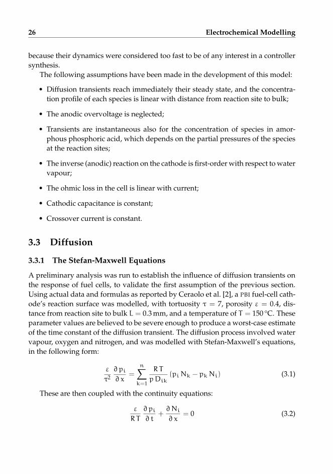
A preliminary analysis was run to establish the influence of diffusion transients onthe response of fuel cells, to validate the first assumption of the previous section.Using actual data and formulas as reported by Ceraolo et al. [2], a PBI fuel-cell cath-ode’s reaction surface was modelled, with tortuosity τ = 7, porosity ε = 0.4, dis-tance from reaction site to bulk L = 0.3 mm, and a temperature of T = 150 °C. Theseparameter values are believed to be severe enough to produce a worst-case estimateof the time constant of the diffusion transient. The diffusion process involved watervapour, oxygen and nitrogen, and was modelled with Stefan-Maxwell’s equations,in the following form:
ε
τ2∂pi
∂ x=
n∑k=1
R T
pDik(piNk − pkNi) (3.1)
These are then coupled with the continuity equations:
ε
R T
∂pi
∂ t+∂Ni
∂ x= 0 (3.2)

3.3. Diffusion 27
OxygenWater
-0.05 0
0.05 0.1
0.15 0.2Time, s 0
0.05 0.1
0.15 0.2
0.25 0.3
Diffusionlayer, mm
4
6
8
10
12
14
16
18
20
22
Partialpressure, kPa
Figure 3.2: Simulated concentration transient on the cathode of a PBI fuel cell; thecurrent steps from 0 to 800 A/m2 at t = 0.
Since diffusion transients are driven by the reactant consumption, they will notin any case be faster than that. If diffusion dynamics is shown to be faster than reac-tant consumption, assuming instantaneous transients for diffusion is an acceptableapproximation.
Furthermore, the diffusion transient can have a noticeable effect on the reactionrate only if the partial pressures at the reaction sites are sufficiently low, that is,when the cell is close to the mass-transport barrier.
The result of diffusion modelling is shown in figure 3.2. This model predictstransients, without overshoots, in the order of 10−1 s in case of steps in the reactionrate1. As long as the time constants of transients in reaction rate are larger than10−1 s, the diffusion transients may safely be assumed to be instantaneous, but theymay be more important when transients in reaction rate are faster.
3.3.2 Simplified Diffusion
To simplify the Stefan-Maxwell equations, we assume that diffusion transients settleimmediately, and that all partial-pressure profiles are linear from bulk to reactionsite. We can then easily integrate:
1We will shortly see that such steps are in fact impossible, since reactant consumption varies con-tinuously as a function of overvoltage.

28 Electrochemical Modelling
pi(x) ' pi,r +∂pi
∂ xx (3.3)
Since the Stefan-Maxwell multicomponent diffusion equation (3.1) is valid forany positive distance x 6 L from the reaction site, we can evaluate it with the bulkvalues of partial pressures, pi,b = pi(L), which are known; furthermore, since weare neglecting the diffusion transient, we can assume that the flows of oxygen, ni-trogen and water will be constant in x and directly related to the reaction currentdensity ir, that is the current corresponding to reactant consumption:
NO2= −
ir
4F(3.4)
NH2O =ir
2F(3.5)
NN2= 0 (3.6)
Inserting this in the Stefan-Maxwell equation (3.1–3.3), the resulting direct for-mulæ are:
pO2,r = pO2,b −L τ2
ε
R T
4 F
(2pO2,b + pH2O,b
pDO2,H2O+
pN2,b
pDO2,N2
)ir (3.7)
pH2O,r = pH2O,b +L τ2
ε
R T
4 F
(2pO2,b + pH2O,b
pDO2,H2O+ 2
pN2,b
pDH2O,N2
)ir (3.8)
It can be seen that, in this approximation, the reaction-site partial pressuresvary linearly with reaction-current density. Incidentally, we can obtain an approxi-mate expression of the current iL at the mass-transport barrier, which occurs whenpO2,r → 0, by rearranging equation 3.7:
iL = pO2,bε
L τ24 FR T
(2pO2,b + pH2O,b
pDO2,H2O+
pN2,b
pDO2,N2
)−1
(3.9)
While this expression is not an exact one, it is very useful as a rough, inexpensiveestimate, and as a first guess in more detailed, iterative solution algorithms.
In equations 3.7, 3.8 and 3.9 the components of group Lτ2
ε always appear to-gether. It is not possible to estimate L, τ and ε separately in this model, so they willbe integrated in a new variable, λ = Lτ2
ε . λ represents the thickness of an equivalentdiffusion layer that would result in the same reaction-site partial pressures as in theporous electrode.

3.3. Diffusion 29
Figure 3.3: Diffusion layer a) has uniform properties and only one value for λ; a reallayer as b) has different properties at different points.
3.3.3 Distributed Layer Thickness
The previous sections implicitly assumed a deterministic value for the effectivethickness λ. However, as illustrated in figure 3.3, the actual picture is more complex.The points on the electrode area have different properties, resulting in different val-ues for λ. As the electrochemical system is a nonlinear function of reaction-sitepartial pressures (and, by equations 3.7 and 3.8, of λ), the shape of the distributionmay influence the overall polarisation curve.
To test this possibility, the model will implement the possibility of using a dis-tributed equivalent layer thickness, Λ, which will follow a lognormal distribution.
The lognormal distribution’s probability density function of a random variableX is usually reported as:
ρ(x) =
1√
2πσY xe−
[ln(x)−µY ]
2σ2Y if x > 0;
0 if x < 0.(3.10)
The mean µY and the variance σ2Y used in equation 3.10 are not the ones of
random variable X, but of the corresponding normal distribution Y = ln(X). Themean µ and variance σ2 of X are instead given by:
µ = eµY+σ2Y2 (3.11)
σ2 = e2µY+σ2Y
(eσ
2Y − 1
)(3.12)
Some lognormal distributions are shown in figure 3.4.It can be noticed how themean does not in general correspond to the maximum in the density function.

30 Electrochemical Modelling
0
0.5
1
1.5
2
2.5
3
3.5
4
4.5
0 0.5 1 1.5 2 2.5 3
Pro
bab
ilit
y d
ensi
ty
x
σ2=0.01
σ2=0.1
σ2=1
Figure 3.4: Some examples of lognormal distributions. All these have a mean valueof 1.
The lognormal distribution, compared to the more common normal distribution,offers the significant advantage of being exactly zero for all λ 6 0, which representphysically meaningless values.
Given a function that depends on the distributed variable Λ, it is possible toobtain its overall value for the whole range of λ values with a weighed integration.For ease of notation, we will indicate this operation with I[ ]:
I[f(Λ)] =
∫∞0f(λ)ρ(λ) d λ (3.13)
3.4 Calculating the Cell Voltage
The steady-state cell voltage is calculated subtracting catalytic and resistive lossesfrom the reversible electrochemical potential:
V = Erev − rMEA (i+ ic) − η (3.14)
The reversible cell potential Erev can be found from well-known thermodynamicdata:

3.4. Calculating the Cell Voltage 31
Erev = −∆g0f
nF+R T
n Fln
(aO2
aH2
aH2O
)(3.15)
∆g0f is calculated at standard conditions, and the activities are those at the re-
action sites. In the case of a distributed Λ, since reaction-site partial pressures andactivities depend on the specific value of λ through equations 3.7 and 3.8, in is nec-essary to integrate the last term:
Erev = −∆g0f
nF+R T
n F
I[ln(aO2
)]
+ I[ln(aH2
)]− I[ln(aH2O)
](3.16)
Erev will in this case be a function of ir and Λ. Note that I may refer, depend-ing on which term is integrated, to the thickness distribution of the cathode or theanode.
The crossover current ic lumps together the parasitic losses, such as electronicconductivity in the membrane. It is generally small, and is important only at lowvalues of current, where it prevents the cell from reaching reversible voltage at opencircuit. Its value is usually assumed constant in the literature.
The ohmic loss is immediately found as the product of the membrane-electrodeassembly’s specific resistance and the sum of circuit and crossover current density,rMEA (i+ ic).
The model is able to simulate overvoltage effects on the anode, but these are ofminor importance in normal operation. They will be therefore neglected, and onlythe cathode will be considered: unless differently specified, it will be understoodfrom now on that all electrochemical terms refer to the cathode.
At steady state, the reaction current density ir is equal to the circuit current den-sity i plus the crossover current density ic; ir represents the reaction rate resultingfrom the Butler-Volmer equation, i the actual current flowing in the external circuitdivided by the cell’s area, and ic the internal losses such as permeation of reactantsthrough the membrane or electronic conductivity of the membrane.
Liu et al. [10] have studied the oxygen reduction reaction at the cathode of aPBI fuel cell. Their results indicate that the rate-determining step is first-order withrespect to oxygen and protons:
O2 + H+ + e− −−→ O2H (3.17)
The remaining steps from O2H to H2O are faster, and can be assumed to beinstantaneous. The oxygen term is the oxygen present in amorphous H3PO4, andthe concentration of protons can be promoted by water:

32 Electrochemical Modelling
H3PO4 + H2O −−−− H2PO−4 + H3O+ (3.18)
In the data range of interest, the data provided by Liu et al. seems to indicatethat the concentration of H+ is approximately proportional to the partial pressureof water vapour.
There are no equivalent studies for the inverse reaction of water oxidation, so itwill be simply assumed to be first-order with respect to water.
12 H2O −−→ H+ + e− + 1
4 O2 (3.19)
Assuming that the activity of oxygen in the amorphous H3PO4 phase is pro-portional to the partial pressure of oxygen at the reaction site (with no transientmodelled), the following expression results for the exchange current density [11]:
i0 = nFk
(pO2
p0
)α (pH2O
p0
) 1+α2
(3.20)
where n is equal to 1 and p0 is the standard pressure (101 325 Pa). Finally, Liuet al. also provided an estimate for the symmetry factor α, in the range 0.42–0.44;α = 0.43 will be assumed.
Reaction current density ir, representing the current corresponding to the reac-tion rate per unit area, can then be calculated for a given activation overvoltage η,which represents the voltage loss associated to reaction kinetics, according to theButler-Volmer equation [11]:
ir = i0
(eα
nFRT η− e−(1−α) nFRT η
)(3.21)
If we are considering a distributed Λ, we would then obtain the value of ir bythe following relationship:
ir(η,Λ) = I[ir(η, λ)] (3.22)
Since equation 3.21, which binds η and the reaction current density ir, cannot beexplicitly inverted directly as η = f(ir), an iterative algorithm is necessary. How-ever, if we assume that the second exponential term in equation 3.21 is much smallerthan the first one, we obtain the Tafel equation:
η =R T
αnFln(ir
i0
)for ir > i0
η = 0 for ir ∈ [0, i0](3.23)

3.5. Dynamics 33
Figure 3.5: Diagram of the fuel-cell model.
The Tafel equation is not very accurate for low values of η and is not invertiblefor ir < i0, but is a very useful, inexpensive estimate in most situations.
3.5 Dynamics
Transients occur when ir 6= i+ i0, because this indicates that there is a charge imbal-ance that will change the value of overvoltage η. The dynamic equation describingthe transient is as follows [2]:
η =i+ ic − ir
C(3.24)
This is the only differential equation that we will consider in order to simulatethe transient of the fuel cell. As already mentioned, all diffusion transients will beneglected, and any capacitance or inductance in any part of the load is neglected aswell. Capacitance C is assumed to be constant, but some authors reported it to bevariable [12]. C represents the sum of an electrostatic double layer capacitance, apseudocapacitance due to charge stored by adsorbed and intermediate products atthe surface, and the charge stored in the diffusion layers [13].
The external load applied to the model is allowed to vary with time, and isdescribed by a function of the form I = f(V , t). It has been chosen to use this forminstead of V = g(I, t) to allow the implementation of loads such as MOSFETs, wherethere can be infinite values of I for one value of V .
Figure 3.5 represents the model graphically. There, one can see the internal resis-tance rMEA, the reversible potential Erev, the capacitor C and its overvoltage η. The

34 Electrochemical Modelling
Overvoltage differential equation η =i+ ic − ir
C(3.24)
Butler-Volmer equation ir = i0
(eα
nFRT η− e−(1−α) nFRT η
)(3.21)
Exchange current density i0 = nFk(pO2,r
p0
)α (pH2O,r
p0
) 1+α2
(3.20)
Oxygen diffusion pO2,r = f(ir,pi,b,Λ, T) (3.7)
Water diffusion pH2O,r = g(ir,pi,b,Λ, T) (3.8)
Table 3.1: Summary of the main equations used in the model.
bipole in parallel with the capacitor is a nonlinear voltage-controlled current gener-ator, which represents the Butler-Volmer law imposing a current ir as a function ofη (and many other parameters, as per equation 3.21). This bipole is often modelledas a nonlinear resistance [5], or a linearised value in an area of interest. Incidentally,ideal generator Erev and resistance rMEA can be viewed as a Thevenin equivalentcircuit.
The actual integration of equation 3.24 is not very simple, since ir is a func-tion of many parameters (including η itself) through the Butler-Volmer equation(3.21). Furthermore, the exchange current density i0 in that equation depends onthe reaction-site concentrations of the reactants (equation 3.20), which, in turn, de-pend on their consumption rate, proportional to ir. An iterative loop, consistingof equations 3.7, 3.8, 3.20 and 3.21, is therefore necessary to calculate ir at all in-tegration steps, and this is the major computational cost of the simulation. Thisphenomenon could be approximated assuming a constant i0, but a separate, em-pirical term should then be introduced in equation 3.14 to model mass-transportlosses. The complete set of equations to solve is summarised in table 3.1.
3.6 Time Constants
Given the state x of a dynamic system, a time constant is the factor τ in the followingdifferential equation:
τ x = −x (3.25)
Forcing terms were neglected in this equation for sake of simplicity. We willnow show how to obtain an analytic relationship for the time constant of the elec-

3.6. Time Constants 35
trochemical transient of fuel cells.The external characteristic is assumed to be a generally nonlinear, purely re-
sistive load of the type V = Ψ(i). The reversible voltage Erev, the cell’s internalresistance rMEA and the crossover current ic are assumed to be constant. The timederivative of the cell’s voltage is then expressed as:
dVd t
=d
d t[Erev − η− rMEA (i+ ic)] = −
dd t
(η+ rMEA i) (3.26)
Since the operating point has to be on the load’s characteristic as well as on thecell’s instantaneous one, we can write:
dVd t
=dΨd t
=dΨd i
(i)d id t
(3.27)
Inserting in equation 3.26 and rearranging:
d id t
= −
[rMEA +
dΨd i
(i)
]−1 dηd t
= −
[rMEA +
dΨd i
(i)
]−1i+ ic − ir
C(3.28)
The overvoltage’s time derivative is:
dηd t
=i+ ic − ir
C=
dηd ir
(ir)d ird t
(3.29)
Rearranging:d ird t
=
[dηd ir
(ir)
]−1i+ ic − ir
C(3.30)
Subtracting equation 3.30 from equation 3.28, we obtain the following relation-ship:
d(i+ ic − ir)
d t= −
1C
[rMEA +
dΨd i
(i)
]−1
+
[dηd ir
(ir)
]−1
︸ ︷︷ ︸1/τ
(i+ ic − ir) (3.31)
Assuming that C and rMEA are constant, that functions Ψ(i) and η(ir, . . .) aregiven, the time “constant” τ depends essentially on i and ir:
τ(i, ir) =C[
rMEA + dΨd i (i)
]−1+[
dηd ir
(ir)]−1 (3.32)
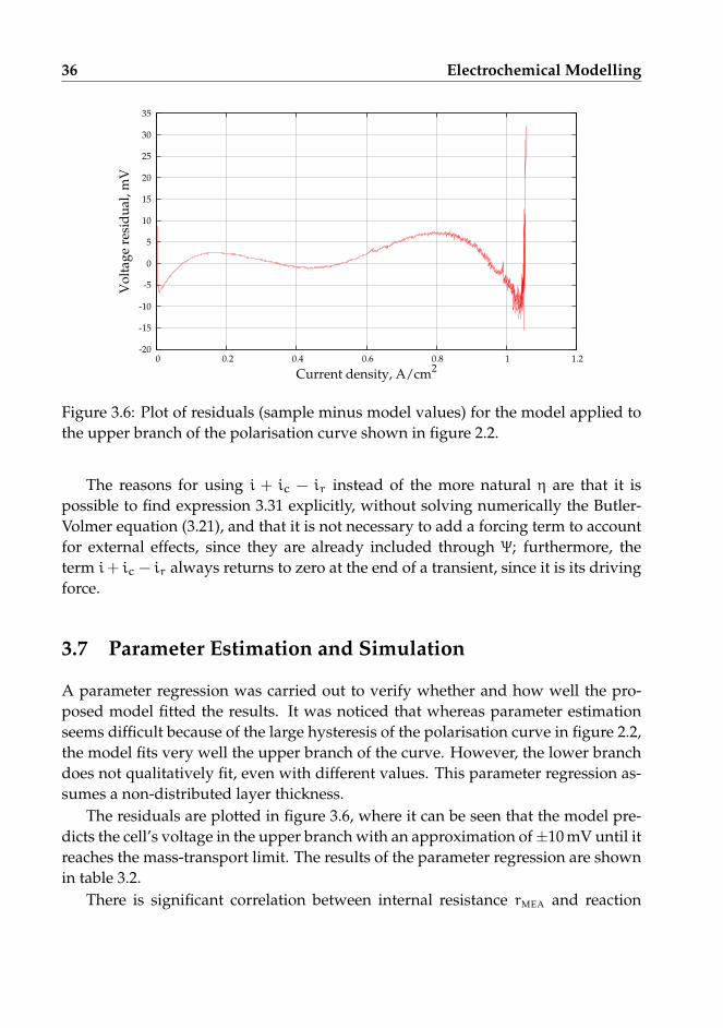
36 Electrochemical Modelling
-20
-15
-10
-5
0
5
10
15
20
25
30
35
0 0.2 0.4 0.6 0.8 1 1.2
Vo
ltag
e re
sid
ual
, mV
Current density, A/cm2
Figure 3.6: Plot of residuals (sample minus model values) for the model applied tothe upper branch of the polarisation curve shown in figure 2.2.
The reasons for using i + ic − ir instead of the more natural η are that it ispossible to find expression 3.31 explicitly, without solving numerically the Butler-Volmer equation (3.21), and that it is not necessary to add a forcing term to accountfor external effects, since they are already included through Ψ; furthermore, theterm i+ ic − ir always returns to zero at the end of a transient, since it is its drivingforce.
3.7 Parameter Estimation and Simulation
A parameter regression was carried out to verify whether and how well the pro-posed model fitted the results. It was noticed that whereas parameter estimationseems difficult because of the large hysteresis of the polarisation curve in figure 2.2,the model fits very well the upper branch of the curve. However, the lower branchdoes not qualitatively fit, even with different values. This parameter regression as-sumes a non-distributed layer thickness.
The residuals are plotted in figure 3.6, where it can be seen that the model pre-dicts the cell’s voltage in the upper branch with an approximation of±10 mV until itreaches the mass-transport limit. The results of the parameter regression are shownin table 3.2.
There is significant correlation between internal resistance rMEA and reaction

3.7. Parameter Estimation and Simulation 37
Estimate Standard Units Correlation matrixdeviation
k 115.7 55.9 µmol/m2 s 1 −0.590 0.672 0.847
λ 25.82 0.349 mm −0.590 1 −0.740 −0.648
ic 33.63 93.94 A/m2 0.672 −0.740 1 0.518
rMEA 26.07 5.96 µΩ m2 0.847 −0.648 0.518 1
Table 3.2: The results of the parameter regression for parameters k, λ, ic and rMEA
with the data of the upper branch of the polarisation curve presented in figure 2.2.
constant k, since in most experimental points the effect of increased resistance issimilar to that of a reduced reaction constant. Similarly, there is high correlation be-tween crossover current density ic and the effective thickness of the diffusion layerλ: since information about λ is gathered mostly at data points close to the mass-transport barrier, an increase in ic will have an effect similar to a reduction in λ,because it will move the barrier to the left in the plot.
To reduce these correlations, one may gather data points from conditions wherethe effects of these parameters are going to vary independently, such as differentvalues of temperature or gas composition.
As noted, the model does not fit the lower branch of the polarisation curve. Itis possible that the lower branch follows different kinetics, or that other factors,such as catalyst deactivation and transients in proton concentration, interfered inthe measurement and caused the hysteresis observable in the scan of figure 2.2.
It was not possible to perform a proper parameter estimation for the cathodiccapacitance, as the slower secondary transients shown in figure 2.5 are not wellunderstood, and would have interfered in the regression procedure. Furthermore,the exact time of switching could not be logged in the measurements with sufficientprecision. However, a value in the range of 1 to 2 kF/m2 seems to reproduce theobserved behaviour with acceptable approximation.
It was found that using a lognormally distributed Λ for the cathode would notresult in an improved fit. The distribution’s standard deviation is very highly cor-related with λ, and the negligible increase in accuracy is considered not to be worththe large overhead in terms of computational effort.

38 Electrochemical Modelling
0.6
0.65
0.7
0.75
0.8
0.85
0 0.02 0.04 0.06 0.08 0.1 0.12 0.14
Vo
ltag
e, V
Current, A
82.25 Ω
5.47 Ω
Polarisation curveResistances
Transient path
Figure 3.7: Simulated transient trying to replicate the experiment in figure 2.4. Thevalue assumed for the capacitance is 1500 F/m2. The markers are spaced by 0.06 s,except those at switching points that are spaced 1 µs.
3.8 Simulation
With the parameters given in table 3.2, a simulation has been carried out to replicatethe experimental measurements of figure 2.4; its results are presented in figure 3.7.
The model allows also to simulate other types of loads, such as MOSFETs. Infigure 3.8, the transient associated to a IRF1404 power MOSFET by InternationalRectifier, Inc. is simulated.
3.9 Impedance Measurements
A common method to extract information from electrochemical systems is measur-ing the electrochemical impedance [14]. With this technique, a fuel cell is initiallykept at a constant base voltage or current, and then small sinusoidal perturbationsof a certain frequency are added. The amplitude ratio and phase shift between volt-age and current oscillations provide a complex function of oscillation frequency,the impedance Z(ω) = R(ω) + iX(ω), whose real part is termed resistance andthe imaginary part reactance. Impedance can also be seen as a transfer functionbetween current and voltage.
The resistance and reactance associated to the model pictured in figure 3.5 arefortunately fairly easy to calculate. For ease of notation, we denote Rc = η/I:

3.9. Impedance Measurements 39
0.6
0.62
0.64
0.66
0.68
0.7
0.72
0.74
0 0.02 0.04 0.06 0.08 0.1 0.12 0.14
Vo
ltag
e, V
Current, A/cm2
Polarisation curve
MOSFET characteristics
Transient path
Figure 3.8: The simulated transient resulting from having changed the gate voltageof a MOSFET from 3.05 to 3.1 volts, when this MOSFET is operating as the load of aPBI fuel cell at 150 °C. The markers are spaced by 0.01 s, except for the switchinginstant when there is a spacing of 1 µs.
R(ω) = RMEA +Rc
1 + (ωRcC)2 (3.33)
−X(ω) =ωR2
cC
1 + (ωRcC)2 (3.34)
These equations do not account for anodic effects and diffusion phenomena; thelatter cannot be modelled explicitly because of the complexity of the Stefan-Maxwellequations. However, in experimental data, a Warburg impedance due to diffusionmay appear at low values of frequency.
We can extract information about RMEA and Rc from an impedance spectroscopyby taking the limits to zero and infinity of the expression given for the cell’s impe-dance:
limω→∞Z(ω) = RMEA (3.35)
limω→0
Z(ω) = RMEA + Rc (3.36)
Calculating the values of impedance for various values of ω, one can plot theimpedance values in the Nyquist plane, as in figure 3.9. The semicircle is a common

40 Electrochemical Modelling
0
0.4
0.8
1.2
0 0.4 0.8 1.2 1.6 2 2.4
−R
ea
cta
nce,
Ω
Resistance, Ω
0.4 V
0.5 V
0.6 V
Figure 3.9: Plot of the impedance of a fuel cell at various values of cell voltage forfrequencies from 10−2 to 103 rad/s. The lowest values of frequency are on the right,and each marker on the curves indicates a ten-fold increase in frequency. Modelparameters are as in table 3.2, cell area is 4 cm2.
result for fuel cells: another (usually much smaller) semicircle may also appear inexperimental data, representing the anode.
Impedance measurements can be a good source of information about the ca-pacitance C of the model: it can be demonstrated that, at the point of minimumreactance (the summit of the semicircle in figure 3.9), the following relation holds:
ωsummit =1RcC
(3.37)
The diameter of the semicircle is Rc; as overvoltage η is not linear with current I,the semicircles will have different diameters for different operating conditions. Atopen circuit, Rc → ∞ since I = 0 and η > 0 (because of the small crossover current):the circle will degenerate into a vertical line passing by R = RMEA.
Since the model can easily calculate the impedance of a fuel cell, it may be possi-ble to perform a parameter estimation for the model’s capacitance C at frequencieswhere the slower transients noticed in figure 2.5 are not important and do not inter-fere with the measurements.

3.10. Instantaneous Characteristics 41
Figure 3.10: The steady-state polarisation curve and the instantaneous characteristicon a V-i plane. The instantaneous characteristic moves up or down depending onthe value of overvoltage η.
3.10 Instantaneous Characteristics
Polarisation curves represent steady-state values2, and do not contain informationabout the way fuel cells behave during transients. To include this information inthe same plot, we define the instantaneous characteristic to be the locus of all pointsin the V-i plane that can be reached instantaneously by the fuel cell. To define it, itis important to examine which terms of the polarisation curve are going to changein a transient, and how so.
The instantaneous characteristic comes from equation 3.14, where the terms Vand i can change stepwise, whereas η evolves dynamically and continuously in timeaccording to equation 3.24. Reaction current density ir, which represents the con-sumption of reactants, is a continuous, strictly increasing function of η, accordingto the Butler-Volmer equation [16]: ir is therefore as continuous in time as η is. Toany value of η corresponds one and one only value of ir, so the state of the fuel cellmay be described by ir just as well as by η: it is possible to express each one as afunction of the other3. The reversible voltage Erev will also not have a discontinuity
2At least ideally so. The slow secondary transients that often appear in laboratory tests (such asthose described by Benziger et al. [15]) are often hidden behind an averaging of the obtained valuesin much of the available literature.
3On the other hand, the Butler-Volmer equation, expressing ir = f(η), cannot be solved explicitlyfor η, and requires an iterative loop. The Tafel equation (3.23) is a very good approximation of η = f(ir)
for sufficiently large values of ir [17].

42 Electrochemical Modelling
Figure 3.11: Transients in the phase plane and in time when stepping (a) the cellcurrent or (b) the cell voltage using a galvanostat or a potentiostat, respectively.
at step time, since it depends on ir.The equation for the cell voltage can be rewritten, highlighting the dynamic and
the algebraic parts:
V(t, i) = Erev − η︸ ︷︷ ︸Vdyn(t)
−rMEA · (i+ ic)︸ ︷︷ ︸Valg(i)
(3.38)
If a stepwise change occurs in i at time t0, Vdyn will remain continuous, and itwill have a single value at that time. Valg will instead change instantaneously withi, and will present a discontinuity.
The instantaneous characteristic described by equation 3.38 can be seen as a linein the V-i plane, rising or descending according to the value of Vdyn(t). It will be astraight line if rMEA is constant, as shown in figure 3.10.
3.10.1 Transient Behaviour
We can now turn our attention to how specific transients develop. The values ofvoltage and current will be determined by the intersection between the instanta-neous characteristics of the cell and the characteristic of the load. If the intersection

3.10. Instantaneous Characteristics 43
Figure 3.12: Transients in the phase plane obtained by changing the external circuit’scharacteristic, on the left with a resistance (stepping from r1 to r2) connected to thefuel cell, and on the right with a MOSFET whose gate voltage is stepped from Vg,1 toVg,2.
point is not on the steady-state polarisation curve, the cell’s instantaneous character-istic will rise or descend until the operating point will be brought to the intersectionbetween the load characteristic and the polarisation curve.
In general, the load may be represented by an instantaneous characteristic aswell, but for ease of treatment we consider only loads with constant characteristics.
In figures 3.11 and 3.12, a few simple transients have been sketched. They allstart from a steady-state point on the polarisation curve, and illustrate the path ofthe operating point to reach the new steady state. All transients can be divided intwo parts:
1. After the step in external load has taken place, the operating point instanta-neously moves to the intersection of the current instantaneous characteristicand the new load;
2. Remaining on the external load’s characteristic, the operating point followsthe movement of the instantaneous characteristic, until it settles on the inter-section between the external load and the polarisation curve.
Whereas the plots in figure 3.11 imply the presence of a current or voltage gener-ator, those in figure 3.12 assume loads that can be changed with little or no external

44 Electrochemical Modelling
power supply. A resistance step may be performed with a simple switch or using arheostat; a step in the gate voltage of a MOSFET4 will require a voltage source, butthis source will have to provide only a negligible amount of power.
3.10.2 Graphical Representation of Time Constants
As previously stated, the catalytic overvoltage varies according to the differentialequation:
dηd t
=i+ ic − ir
C=i− (ir − ic)
C(3.39)
Since the level of the instantaneous characteristic is determined by the valueof η, the right-hand side in equation 3.39 represents also the “speed” at which theinstantaneous characteristics moves vertically on the plot. It is relatively easy tofind i and ir − ic graphically: the circuit current, i, is at the intersection of theinstantaneous characteristic with the external load; the reaction current minus thecrossover current, ir − ic, is at the intersection of the instantaneous characteristicwith the polarisation curve.
The latter claim can be demonstrated as follows: the polarisation curve rep-resents the steady-state points, and the instantaneous-characteristic represents allpoints with the same η and ir: their intersection is the steady state with the samereaction current ir of the transient operating point. Since at steady state, by equa-tion 3.24, ir − ic = i, the projection of this intersection on the i axis is ir − ic, asillustrated in figure 3.13.
An interesting side effect is that some transients may have different time con-stants depending on how “close” to the polarisation curve their trajectory is. If atransient trajectory consists of points “close” to the polarisation curve5, the drivingforce of equation 3.39 (that is i− (ir − ic)) is small, and the transient will be slower.This has been verified experimentally [19], and simulation indicates that times inthe order of 10 s are common to reach steady state in open circuit. Settling times formost transients are in the range between 0.1 and 10 s.
4For a process engineer, MOSFETs can be thought as valves that allow more current through themwhen their gate voltage is increased. For a detailed treatise of MOSFETs, see e.g. Mohan et al. [18].
5More rigorously: points lying on an instantaneous characteristic whose intersection with the po-larisation curve is close, with distance being measured along the i axis.
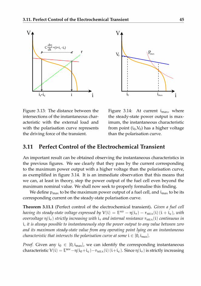
3.11. Perfect Control of the Electrochemical Transient 45
Figure 3.13: The distance between theintersections of the instantaneous char-acteristic with the external load andwith the polarisation curve representsthe driving force of the transient.
Figure 3.14: At current imax, wherethe steady-state power output is max-imum, the instantaneous characteristicfrom point (i0,V0) has a higher voltagethan the polarisation curve.
3.11 Perfect Control of the Electrochemical Transient
An important result can be obtained observing the instantaneous characteristics inthe previous figures. We see clearly that they pass by the current correspondingto the maximum power output with a higher voltage than the polarisation curve,as exemplified in figure 3.14. It is an immediate observation that this means thatwe can, at least in theory, step the power output of the fuel cell even beyond themaximum nominal value. We shall now seek to properly formalise this finding.
We define pmax to be the maximum power output of a fuel cell, and imax to be itscorresponding current on the steady-state polarisation curve.
Theorem 3.11.1 (Perfect control of the electrochemical transient). Given a fuel cellhaving its steady-state voltage expressed by V(i) = Erev − η(ir) − rMEA(i) (i + ic), withovervoltage η(ir) strictly increasing with ir and internal resistance rMEA(i) continuous ini, it is always possible to instantaneously step the power output to any value between zeroand its maximum steady-state value from any operating point lying on an instantaneouscharacteristic that intersects the polarisation curve at some i ∈ [0, imax].
Proof. Given any i0 ∈ [0, imax], we can identify the corresponding instantaneouscharacteristic V(i) = Erev−η(i0+ic)−rMEA(i) (i+ic). Since η(ir) is strictly increasing

46 Electrochemical Modelling
with ir, η(imax + ic) > η(i0 + ic).Subtracting the steady-state characteristic from the instantaneous one at i =
imax, we obtain −η(i0 + ic) + η(imax + ic) > 0, meaning that the instantaneouscharacteristic will have a higher voltage at i = imax, and thereby a larger poweroutput than the steady-state characteristic.
Power along the instantaneous characteristic varies continuously, according tothe formula p(i) = V(i) i, because rMEA(i) is also assumed continuous. It is trivialthat power output can be set to zero by choosing i = 0. For the intermediate-valueproperty, ∃ i : p(i) = p,∀p ∈ [0,pmax].
This theorem guarantees, therefore, that there is a way to immediately change toany value of power output in the complete power range of the fuel cell, from zero tomaximum, under very general conditions. This means there is no inherent limita-tion to how fast control we can achieve in the electrochemical domain, even thoughpractical issues such as measurement time and computation time will eventuallypose a limit.
This has also other implications: if incorrectly controlled, a fuel cell might ex-hibit large spikes in power output, which may damage equipment connected to it.This might be especially important in microelectronics appliances.
3.11.1 Implicit Limitations
Theorem 3.11.1 delivers an important result, but makes some implicit assumptions.The assumption about the form of the function describing the polarisation curve isespecially important, since the curve is expected to be only a function of the cir-cuit and reaction currents: other factors such as temperature, catalyst poisoning,reactant concentration are left out.
Therefore, the theorem is valid only in the context of a certain set of states that definethe polarisation curve: we are only guaranteed that we can instantly reach the max-imum power output for those conditions of temperature, composition, and othervariables defining the cell’s state. This may be less than the nominal power out-put that the fuel cell is supposed to deliver in design conditions. In such a case,other control variables may be used to modify these states, and might pose someperformance limits: for instance, a temperature increase cannot occur stepwise.
3.12 Conclusions
A dynamic model for fuel cells has been developed in this chapter. After evalu-ating the effect of diffusion of reactants through a porous layer, it was concluded

Bibliography 47
that transients in diffusion may be safely assumed to be instantaneous. The datagathered in chapter 2 can be fit with four parameters for steady-state simulation,namely reaction constant and equivalent layer thickness of the cathode, crossovercurrent, and specific ohmic resistance. The possibility of simulating a distributedlayer thickness was added, but it appears that its effect is too small to significantlyimprove the model’s fit. Furthermore, it has a heavy computational cost.
The dynamic part of the model included only the overvoltage transient, becauseit is considered to be the most important. This transient frequently results in over-shoots in power output. It was not possible to make a precise parameter regressionfor the model’s capacitance as secondary unmodelled dynamics would have dis-turbed the result. In future works, impedance spectroscopy may be used to estimatethis parameter in frequency ranges where the secondary dynamics do not interferewith measurements.
The overvoltage transient was illustrated graphically by introducing the conceptof instantaneous characteristic, which has been used to explain qualitatively theshape of some transients. A theorem was demonstrated to show how the powerovershoot associated to the overvoltage transient can make perfect control of thepower output theoretically possible.
Bibliography
[1] Jay B. Benziger, I. G. Kevrekidis, M. B. Satterfield, W. H. J. Hogarth, and J. P. Nehlsen.The power performance curve for engineering analysis of a fuel cell. In AIChE AnnualMeeting, 2005.
[2] M. Ceraolo, C. Miulli, and A. Pozio. Modelling static and dynamic behaviour of protonexchange membrane fuel cells on the basis of electro-chemical description. Journal ofPower Sources, 113:131–144, 2003.
[3] Sampath Yerramalla, Ased Davari, Ali Feliachi, and Tamal Biswas. Modeling and sim-ulation of the dynamic behaviour of a polymer electrolyte membrane fuel cell. Journalof Power Sources, 124:104–113, 2003.
[4] U. Krewer, T. Schultz, and K. Sundmacher. Direct methanol polymer electrolyte fuelcell: Transfer function analysis of current-voltage dynamics. In Fuel Cell Research Sym-posium: Modeling and Experimental Validation. Swiss Federal Institute of Technology,March 2004. http://www.energie-schweiz.ch/internet/03309/index.html.
[5] P. R. Pathapati, X. Xue, and J. Tang. A new dynamic model for predicting transientphenomena in a PEM fuel cell system. Renewable energy, 30:1–22, 2005.

48 Electrochemical Modelling
[6] J. C. Amphlett, R. F. Mann, B. A. Peppley, P. R. Roberge, and A. Rodrigues. A modelpredicting transient responses of proton exchange membrane fuel cells. Journal of PowerSources, 61:183–188, 1996.
[7] Zijad Lemeš, Andreas Vath, Th. Hartkopf, and H. Mäncher. Dynamic fuel cell modelsand their application in hardware in the loop simulation. Journal of Power Sources, 154:386–393, 2006.
[8] Yuyao Shan and Song-Yul Choe. A high dynamic PEM fuel cell model with tempera-ture effects. Journal of Power Sources, 145:30–39, 2005.
[9] Federico Zenith, Helge Weydahl, Ingrid Anne Lervik, Trygve Burchardt, SteffenMøller-Holst, Sigurd Skogestad, and Georg Hagen. Modelling and experimental studyof the transient response of fuel cells. In 9th Ulm ElectroChemical Talks, pages 82–83, 2004.
[10] Zhenyu Liu, Jesse S. Wainright, Morton H. Litt, and Robert F. Savinell. Study of theoxygen reduction reaction (ORR) at Pt interfaced with phosphoric acid doped poly-benzimidazole at elevated temperature and low relative humidity. Electrochimica Acta,51:3914–3923, 2005.
[11] John Newman and Karen E. Thomas-Alyea. Electrochemical Systems, chapter 8: Modelsfor Electrode Kinetics, pages 212–213. John Wiley & Sons, 3rd edition, 2004.
[12] Arvind Parthasarathy, Bhasker Davé, Supramaniam Srinivasan, A. John Appleby, andCharles R. Martin. The platinum microelectrode/Nafion interface: An electrochemicalimpedance spectroscopic analysis of oxygen reduction kinetics and Nafion character-istics. Journal of the Electrochemical Society, 139(6):1634–1641, June 1992.
[13] John Newman and Karen E. Thomas-Alyea. Electrochemical Systems. John Wiley &Sons, 3rd edition, 2004.
[14] J. Ross Macdonald and William R. Kenan. Impedance Spectroscopy, emphasizing solidmaterials and systems. Wiley-Interscience, 1987.
[15] Jay Benziger, E. Chia, J. F. Moxley, and I.G. Kevrekidis. The dynamic response of PEMfuel cells to changes in load. Chemical Engineering Science, 60:1743–1759, 2005.
[16] Carl H. Hamann, Andrew Hamnet, and Wolf Vielstich. Electrochemistry. Wiley-VCH,1998.
[17] James Larminie and Andrew Dicks. Fuel Cell Systems Explained. Wiley, 1st edition, 1999.
[18] Ned Mohan, Tore M. Undeland, and William P. Robbins. Power Electronics: Converters,Applications and Design. John Wiley & Sons, Inc., 2nd edition, 1995.
[19] Federico Zenith, Frode Seland, Ole Edvard Kongstein, Børre Børresen, Reidar Tunold,and Sigurd Skogestad. Control-oriented modelling and experimental study of the tran-sient response of a high-temperature polymer fuel cell. Journal of Power Sources, 162(1):215–227, 2006.

Chapter 4
Mass and Energy Modelling
Most dynamic models of fuel cells published in the open literature are based onmass and energy balances. Some of these are very detailed in the phenomena theymodel, and there are also applications of computational fluid dynamics to obtaintwo- or three-dimensional simulations in which temperature, compositions, pres-sure and current density can have variable values in every point of the fuel cell.
These studies are of high value, but are also computationally demanding. Asthis thesis is concerned with control of fuel cells, a simpler model will be presented.The goal of this model, rather than high accuracy, is to present the essential dy-namic phenomena of interest for control. For this simpler task, a lumped (zero-dimensional) model with some simplifying assumptions was chosen. Any devia-tions between the simple model and the real behaviour of the fuel cell may be takencare of by a feedback loop in the control system.
4.1 Literature Review
One of the first dynamic models for fuel-cell systems was published in the litera-ture by He [1] in 1994. He considered a molten-carbonate fuel-cell stack fed withreformate hydrogen, and focused mostly on mass flows and energy balance of thepre-processing plant and of the cell stack. The electrochemical model was com-paratively simple, with no dynamics and being, essentially, a Thevenin equivalentcircuit with a voltage generator and a resistance.
A dynamic model for PEM fuel cells by Amphlett et al. [2] appeared in 1996, andwas subsequently quoted in a large number of papers. It was a thermal model witha basic, empirical modelling of the overvoltage effects. Current was considereda system input, and the catalytic overvoltage was assumed to vary instantly as a
49

50 Mass and Energy Modelling
Figure 4.1: A possible configuration for the reactant flows of a fuel cell. The anodicflow is pure hydrogen and is dead-ended, whereas the cathodic flow is atmosphericair and has an exhaust to take out water and nitrogen as oxygen in replenished.
function of temperature, oxygen concentration and current. The model predictswell the behaviour of the stack in a time scale of minutes, but, since it does notconsider the transient in overvoltage, it might be less accurate in the scale of secondsand lower.
The issue of managing the water-content dynamics in Nafion membranes wasrecognized by van Bussel et al. [3], who identified the possibility of great variationsin current density in the same cell when operated on dry gases, and stressed thebeneficial effect of higher water content in the anode gas.
The model presented by Meng and Wang [4] provided a detailed simulation offlows in three dimensions using computational fluid dynamics. Their model in-cluded transients in reactant concentration in bulk and diffusion layers for bothelectrodes, water production, diffusion and electro-osmosis, but it did not includethe overvoltage transient. Similar models have been proposed by Nguyen et al. [5]and Zou et al. [6].
A three-dimensional dynamic model focused on water transport has been stud-ied by Wang and Wang [7, 8]. They concluded that anode back-diffusion would takesome seconds to compensate for an anodic dry-out caused by an increase in current,causing significant voltage losses at the anode. In extreme conditions, these lossesmay reverse the cell voltage. Gas-diffusion transient were found to be much faster,in the range of 10−1 to 10−2 s.

4.2. Mass Balances 51
4.2 Mass Balances
Of the many possible flow configurations to deliver reactants to a fuel cell, the onechosen for this thesis is shown in figure 4.1. The essential difference between fuelcells and batteries is that fuel cells have a continuous feed of fuel and oxidant (forexample hydrogen and air), whereas batteries contain the reactants themselves. Therequirement on the presence of species is twofold:
1. Mass balances require that a sufficient amount of reactants is present in bothelectrodes of the fuel cell to sustain the reaction;
2. Reaction kinetics requires reactants to be present in concentrations higher thana certain threshold, ideally as high as possible, in order to reduce the catalyticlosses in voltage and increase efficiency.
As expressed by equation 3.20, the exchange current density depends on thepresence of reactants, and possibly other species. Any variation in exchange currentdensity i0 is going to be directly mirrored into the reaction current density ir, sincethe Butler-Volmer equation (3.21) states that ir ∝ i0. In fact, the expression forexchange current density is the one and only point where the electrochemical modelpresented in chapter 3 interacts with reactant concentration.
Gases are usually fed into a fuel-cell stack through a manifold from which thegases can enter the single cells. The cells may be connected in parallel, with a singlemanifold connecting all the cells, or in series, with each cell’s outlet feeding the nextcell’s inlet, or a mixture of these approaches, possibly with many smaller manifoldsspanning a certain number of cells. If the gas entering a manifold contains inertcomponents, or if reaction products are going to appear on that side of the cell, anexit manifold will be required. We will first consider the mass and energy balancesfor a single cell, and we will then look at how the manifold layouts influence ouranalysis.
4.2.1 Dead-End Flows
Some gas flows do not need an outlet, since all of the entering flow is going to beconsumed and no products will be generated on that side of the fuel cell. This isgenerally the case of pure hydrogen fed to the anode of PEM fuel cells. In the caseof Nafion membranes, hydrogen may also be humidified to improve membraneconductivity and avoid dry-out, and water will permeate to the cathode along withthe protons.

52 Mass and Energy Modelling
For the case of an anode fed on pure hydrogen, the equation of mass conserva-tion is simply:
dnH2
d t= nH2
−irA
2 F(4.1)
Assuming that the ideal gas law is valid, nH2=pH2
V
RT , which after derivationgives:
dnH2
d t=
V
R T
(dpH2
d t−pH2
T
d Td t
)(4.2)
Inserting expression 4.1 and rearranging as a dynamic equation of pressure:
dpH2
d t=R T
V
(nH2
−irA
2 F
)+pH2
T
d Td t
(4.3)
The last term may be neglected if temperature transients are sufficiently slow,since transients in pressure are typically faster than ones in temperature.
In a real system there are always some impurities associated with hydrogen:therefore, some form of periodic purging will be necessary even for dead-end flows.This has not been modelled here because it is assumed to be a discontinuous and rel-atively rapid process. If the fraction of impurities in the entering flow is significant,an open-end flow layout may be more appropriate.
4.2.2 Open-End Flows
When flows passing through the fuel cell contain inert components, poisons, orreceive some reaction products such as water, they require an outlet to remove thesenon-reacting species.
In all types of PEM fuel cells, this is always the case for cathodic gases, as waterforms on the cathode and must be disposed of. In the important case of air-fedcells, inerts in the form of nitrogen represent almost 80 % of the entering molar flow,and in addition to that comes air humidity. This is also the case for anodic gaseswhenever hydrogen is not pure, for instance when hydrogen gas has been producedby a reformer and is still contains amounts of carbon oxides and water vapour.
Diffusion Limits
The main problem posed by inert gases is the appearance of diffusion limits. Sim-plifying the Stefan-Maxwell equations, an approximate limit to the reaction currenthas been obtained in equation 3.9, considering only the cathode. At this limiting

4.2. Mass Balances 53
current, the steady-state partial pressure of oxygen at the reaction surface reacheszero: this limit is often named the mass-transport barrier in the literature.
The limiting current, as can be seen in equation 3.9, is proportional to the partialpressure of oxygen in the bulk (outside the diffusion layer) for small oxygen con-centrations. When oxygen is more dominant, the dependence becomes weaker, andeventually disappears when pure hydrogen is fed and pH2O,b = pN2,b = 0. Even ifthe cell is fed pure oxygen, however, the mass-transport barrier will not disappear,as water still has to exit the diffusion layer. To move the current limit to higher val-ues and allow more power output from the cell, therefore, it is necessary to increasethe fraction of oxygen in the cathode gases. The simplest approach is to increase theinlet flow to purge inerts and bring oxygen closer to its inlet concentration.
For the case of an impure hydrogen flow on the anodic side, in presence of CO,CO2 and H2O (as would be the case for the outlet of a hydrocarbon reformer), anexpression similar to equation 3.9 can be derived:
iL,a = pH2,b2 FλR T
(pCO,b
pDH2,CO+
pCO2,b
pDH2,CO2
+pH2O,b
pDH2,H2O
)−1
(4.4)
Again, to increase the current limit one would have to increase the partial pres-sure of hydrogen in the bulk gas, pH2,b. However, whereas air is obtained for freefrom the environment, the anode exhaust gases would still contain valuable hydro-gen. Therefore, when operating open-ended, the anode outlet may deliver gas to autility that may make use of it, such a gas turbine, a burner for a heating unit, ora purifying unit from which the remaining hydrogen can be extracted and recycledback to the anode.
Effects of Bulk Oxygen Concentration
As the partial pressure of oxygen in the cathode’s bulk influences the shape of thecell’s polarisation curve, a series of simulations has been performed with parame-ters from table 3.2 to determine its effect.
The composition of air in a fuel cell’s cathode changes as oxygen reacts withhydrogen to form water vapour. For a given oxygen conversion, the number ofmoles for the three gas species considered (oxygen, nitrogen and water) and theirtotal is:

54 Mass and Energy Modelling
nO2= n0
O2(1 − X)
nN2= n0
N2
nH2O = n0H2O + 2Xn0
O2∑i
ni =∑i
n0i + Xn0
O2
(4.5)
Where X is conversion and n0i is the initial number of moles of generic species i.
Since the molar fraction of a generic species i is by definition xi = ni∑ini
, the molarfractions will be a function of conversion according to the following relations:
xO2=x0
O2(1 − X)
1 + x0O2X
xN2=
x0N2
1 + x0O2X
xH2O =x0
H2O + 2 x0O2X
1 + x0O2X
(4.6)
We will assume that the initial feed has a total pressure of 101 325 Pa (a standardatmosphere). The partial pressure of water is assumed to correspond to 1700 Pa, thevapour pressure of water at approximately 15 °C, or a relative humidity of 53 % at25 °C. The remaining dry air is assumed to be made up of 20 % oxygen and 80 %nitrogen.
With various values of X, the polarisation curve calculated with equation 3.14changes as shown in figure 4.2. It is noticeable how the mass-transport barrier re-cedes almost linearly with conversion, and that some conversion is actually benefi-cial at low currents: the reason is that an increase in water vapour will increase theexchange current density (3.20), actually promoting the reaction. This latter positiveeffect is however limited in extent.
The maximum power outputs for the polarisation curves of figure 4.2 are shownin figure 4.3 as a function of conversion, along with the corresponding oxygen andwater molar fractions. It is noticeable how the maximum available power variesalmost linearly with all of these variables.
These results are valid for a fuel cell whose cathodic bulk partial pressures areas given by equation set 4.6. This is the case for a fuel cell whose open-end cath-ode manifold operates as a steady-state CSTR (with perfect mixing), and with noperturbations in the entering composition.

4.2. Mass Balances 55
0
0.1
0.2
0.3
0.4
0.5
0.6
0.7
0.8
0.9
0 500 1000 1500 2000 2500 3000
Vo
ltag
e, V
Current density, A/m2
X = 0.0
X = 0.1
X = 0.2
X = 0.3
X = 0.4
X = 0.5
X = 0.6
X = 0.7
X = 0.8
X = 0.9
Figure 4.2: Polarisation curves of a fuel cell as oxygen conversion advances due tothe reaction. The cell’s parameters are those reported in table 3.2.
0
0.2
0.4
0.6
0.8
1
0 200 400 600 800 1000
Maximum power density, W/m2
Conversion
Fraction of oxygen
Fraction of water vapour
Figure 4.3: The maximum allowable conversion in the cathode’s bulk (with corre-sponding molar fractions of oxygen and water vapour) for various levels of poweroutput from a fuel cell.

56 Mass and Energy Modelling
Figure 4.3 can therefore be used to derive a simple rule-of-thumb for fuel cells ofthe type investigated in this thesis: a fuel cell’s maximum power output is approxi-mately proportional to oxygen partial pressure. This implies that the air flow in thecathode should be large in order to produce more power.
Mass-Balance Equations for Open-End Flows
For a generic species i, the dynamic mole balance in an open-end flow is:
dnid t
= nin xini − nout xi + νi
irA
F(4.7)
The stoichiometric factor νi indicates how many moles of the species are pro-duced or consumed for every mole of electrons transferred. Since the anodic andcathodic reactions are, respectively:
12 H2 −−→ H+ + e−
14 O2 + H+ + e− −−→ 1
2 H2O(4.8)
we have that νO2= −1
4 , νH2= −1
2 , νH2O = 12 and νN2
= 0.When pressure is constant, the total outlet molar flow depends only on the tran-
sients in reaction rate and temperature, and can be calculated by the following rela-tion:
nout = nin +
Reaction︷ ︸︸ ︷∑i
νiirA
F+
Heat expansion︷ ︸︸ ︷pV
R T 2d Td t
(4.9)
Inserting this expression for nout into equation 4.7 and assuming constant pres-sure, the molar balance becomes:
pV
R T
d xid t
−
xipV
R T 2d Td t
= nin (xini − xi
)+irA
F
νi − xi∑j
νj
−
xipV
R T 2d Td t
pV
R T
d xid t
= nin (xini − xi
)+irA
F
νi − xi∑j
νj
(4.10)
Fortunately, the heat expansion term cancels out when expressing the dynamicsin terms of molar fraction rather than number of moles. This is a series of differ-ential equations in molar fractions xi. In a control setting, we can view nin as the

4.3. Energy Balance 57
manipulated variable, since it can be set with an air blower or a compressor, and iras a disturbance, since it is a consequence of the external load connected to the fuelcell. It is well worth remarking that this system is nonlinear.
4.3 Energy Balance
Energy balance and temperature dynamics are important topics for PEM fuel cells.Nafion-based PEM cells operate in a narrow temperature range, usually around80 °C (more if pressurised), whereas PBI membranes can operate in a range span-ning from 125 to 200 °C. High temperatures may be exploited to reduce the catalyticovervoltage by increasing the value of reaction constant k in table 3.2, or to increasetolerance to catalyst poisons such as CO.
Temperature control in Nafion-based PEM cells is usually taken care of by a ded-icated cooling system for all but the smallest cell stacks [9]. This cooling systemrequires additional channels to be machined out in the cell’s bipolar plates, whichare the most expensive part of a fuel cell [9], adding to their cost and complicatingdesign. The necessity of such a cooling system arises from the low temperatures ofexhaust gases, which reduce their associated enthalpy flow, making it difficult toremove all the heat generated by the cell only by means of the exhaust flows.
4.3.1 Air Cooling
Fuel cells with PBI instead of Nafion as membrane material operate at higher tem-peratures, and the need for of a separate cooling system could be eliminated bysimply feeding the cell stack additional air at ambient temperature [10]. To quicklyverify this possibility, we will consider a simple back-of-the-envelope calculationfor the case of maximum power output from a PBI fuel cell with parameters fromtable 3.2, at 150 °C and fed with pure hydrogen and dry air at standard ambienttemperature (25 °C). Our goal is to find out what air excess ratio, defined as theratio of air fed to the cell versus the required stoichiometric air flow, is necessary toremove all produced heat at the operating point of maximum power output1.
The overall reaction in the fuel cell is the well-known oxidation of hydrogen:
H2 + 12 O2 −−−− H2O(g) (4.11)
As shown in figure 4.3, the maximum electric power output is about 1 kW/m2;the corresponding polarisation curve in figure 4.2 indicates a voltage of about 0.35 V
1Since the maximum power output is also the point of minimum efficiency for normal operationof fuel cells, it will also be the point of maximum heat output.

58 Mass and Energy Modelling
at maximum power. The standard enthalpy of reaction 4.11 does not change muchwith temperature, and in the temperature range we are interested in (125 to 200 °C)it is about ∆h0
r ≈ −243 kJ/mol. As the energy we are taking out of the system aselectric power is 0.35 V×2 F = 67.5 kJ/mol, a cell at maximum electric power outputwill produce about 175 kJ/mol of heat.
The stoichiometric quantity of air for the reaction is 2.5 moles per mole of prod-uct water, as 0.5 moles of oxygen are required by reaction 4.11. The heat capacity ofair in the temperature range of interest is about 30 J/mol K. Assuming that air en-ters the cell at a standard temperature of 25 °C and leaves it at 150 °C, and that thereaction of oxygen to water does not significantly alter the flow’s heat capacity, a sto-ichiometric air flow will remove 30 J/mol K×2.5 molair
molH2O×(1 50 − 25) K = 9375 J/mol
from the cell. The air excess ratio that will dissipate the cell’s heat output will thenbe about 175000
9375 ≈ 18.6. Whereas this value may appear high, it is not unusual forfuel cells [9], and will be required only in the case of maximum power output.
This approximate calculation has shown that cooling a PBI fuel-cell stack by us-ing only air as a cooling medium is possible.
4.3.2 External Heating for Cold Start-up
When the stack is at low temperatures, typically at start-up, it might be difficultto bring it to operational temperature, as the reaction cannot proceed at too lowtemperatures and internal heat generation is therefore not possible.
In order to provide a separate heat input, we will consider the possibility ofinjecting and burning hydrogen in the air inlet stream to raise its temperature. Thismethod is wasteful of hydrogen, but has the benefit of simplicity in analysis andrealisation, and delivers heat directly where it is needed (the cathode’s reactants),instead of heating first the whole stack and its plates. This layout is presented infigure 4.4.
4.3.3 Enthalpy-Balance Equations
The main sources and sinks of heat for the fuel cell of figure 4.4 are entering andexiting flows, the heat generated by the cell, and losses to the environment. Anenthalpy balance around the stack and the burner yields:
dHd t
= Hin − Hout −
Electric power︷ ︸︸ ︷ir V A −Hloss (4.12)
This simple model assumes only one temperature to be representative of the

4.3. Energy Balance 59
Figure 4.4: Flow layout for a PBI fuel cell with air cooling and heating with hydrogencombustion.
whole cell. Indeed, according to results published by Shan and Choe [11], temper-atures across the various elements of a cell (plates, gas channels, MEA) tend to befairly uniform. In fact, in a later study, the same authors [12] noted that the temper-ature in a whole stack is quite uniform, with the exception of the cells at the ends ofthe stack. Their studies were however focused on low-temperature PEM fuel cells,and should be verified for PBI membranes.
The relationship between enthalpy content of a cell and its temperature may beextracted by data published in the literature [11], where one can find that the heatcapacity per cell area is about 7 kJ/K m2. It is therefore:
dHd t
= A cpd Td t
(4.13)
The entering enthalpy flow also contains the heat generated by the combustionof hydrogen when heating of the cell is required, as for example in a cold start. Itwill therefore be equal to the enthalpy associated to the ambient air plus the enteringhydrogen flow:
Hin = nair hair(T0) +(nH2
+ ncH2
)hH2
(TH2
)(4.14)
Temperature TH2may be significantly different from ambient temperature T0, as
hydrogen from storage may undergo a significant expansion, be evaporated fromliquid state, or heated in order to dissociate it from hydrides. Modelling the dy-namics of hydrogen inlet temperature is beyond the scope of this thesis, and wewill assume that hydrogen has been brought to ambient conditions, and that there-fore TH2
= T0.

60 Mass and Energy Modelling
We assumed that the only output in our fuel cell is the cathode’s. The cathodegas composition will change as oxygen is consumed, and the total outlet molar flowwill be larger or equal than the entering one.
Hout =∑i
nouti hi(T) (4.15)
nouti represents the sum of the entering flow of species i, nin
i , plus the moles cre-ated (or minus the ones consumed) by the reaction between hydrogen and oxygen.Lastly, there is a small effect of thermal expansion of gases if temperature is varying.If pressure is constant, the outlet molar flow for species i is:
nouti =
Entering︷︸︸︷nini +
Reaction with H2︷ ︸︸ ︷νi
(ncH2
+irA
2 F
)+
Heat expansion︷ ︸︸ ︷xipV
R T 2d Td t
(4.16)
The functions hi(T) depend on the temperature T of the cell’s cathode.The heat loss to the environment, Hloss, would generally be a beneficial factor as
the main issue in a functioning PBI fuel-cell stack would be removing heat from thestack rather than withholding it. However, its actual expression will depend on thestack materials and layout: for sake of simplicity, we will assume Hloss = 0.
4.4 Cell Stacks
As fuel cells can produce only limited voltages, usually below 1 V, the obviousmethod to electrically connect a stack of fuel cells is to connect them in series, toproduce larger voltages.
Other networks in need of a layout are the ones used to deliver the reactants atcathodes and anodes. The flows can be arranged in series through all cells, or witha common manifold for all cell inlets, or with a combination of these.
The series flow layout guarantees that the same flow rate will pass through allcells, and obstacles to flow, such as liquid water accumulation in Nafion-based cells,can be removed mechanically by the flow itself. With a parallel layout, instead, thecell in which liquid water accumulates would cause more resistance to flow, leadingto less flow in the cell, less water removal, and lower concentration of reactants thatmight even deplete. In these conditions, reaction would halt in the cell: this hasfar-reaching consequences, as the current through the whole stack would be halted,since the stack is still electrically connected in series.
However, since the series flow layout assumes that all the flow will pass througheach cell, the stack’s pressure drop will rapidly increase with the number of cells.

4.4. Cell Stacks 61
Figure 4.5: Various arrangements of the air flow through a fuel-cell stack: a) parallelflow, b) serial flow, and c) sequentially exhausted flow [13].
If a parallel-connected stack has a pressure drop ∆pparallel, the pressure drop of thesame stack, with a series flow layout and the same total stack flow, will have to bemultiplied with the number of cells n, as the pressure drop through the n cells willsum up from stack inlet to stack outlet, and with its square n2, since the flow of all ncell will pass through each cell and pressure drop increases roughly with the squareof flow. Therefore, the pressure drop of series-connected stacks will be much higherthan for parallel-connected ones:
∆pseries ≈ n3∆pparallel (4.17)
For a stack of 50 cells, not a particularly large number, the series layout’s pres-sure drop will be an impressive 125 000 times the pressure drop of an equivalentparallel-connected stack. Furthermore, the series flow will change its composi-tion and temperature while travelling through the cells, collecting heat and reactionproducts, and causing each cell to be under different conditions. These limitationsof series-flow arrangements were already apparent to Litz and Kordesch [14] in1965, and series layouts are therefore applied in shorter stacks only, such as thoseinvestigated by Dhathathreyan et al. [15]. In larger stacks, such as those that couldbe used in vehicles, compression costs represent the main energy losses of ancillaryplants in the system [16], and a large increase in pressure drop is unacceptable.
Nafion-based PEM fuel-cell stacks need the qualities of both layouts: the water-removal capability of the series layout and the scalability of the parallel layout.Nguyen and Knobbe [13] devised a conceptually simple approach where cells aresequentially exhausted, so that liquid water accumulation is staved off and the gasstream must not travel needlessly through all cells; however, this requires a seriesof regulating valves for each cell. As the cells operate batch-wise between each wa-ter purging, the frequency of this water purging must be sufficiently rapid so thatoxygen is not depleted: with large stacks and high currents, the required switching

62 Mass and Energy Modelling
Figure 4.6: The flow layout considered in this thesis, here exemplified for a three-cellstack.
rate may prove to be very high and unpractical. This approach was further refinedby Knobbe et al. [17], who suggested installing a separate valve at the outlet of eachcell, and the possibility of purging the cells by group rather than one by one. Themain categories of flow layouts are sketched in figure 4.5.
PBI-based PEM fuel cells, instead, do not require any water management, andcan be stacked with much simpler parallel layouts for both anodic and cathodicflows. Karimi et al. [18] have investigated various possible layouts for parallel flowin fuel cells, simulating the pressure drop and voltage spread of a 51-cell stack withdifferent inlet and outlet positionings; they found that one of the best layouts withsingle inlet and outlet is the Z configuration, where the outlet is on the opposite sideof the stack relative to the inlet.
The overall flow network assumed in this thesis is shown in figure 4.6. Hy-drogen is fed in parallel to the cell anodes, whereas the air network (possibly afterburning some hydrogen for heating) is arranged in a Z configuration.
Bibliography
[1] Wei He. A simulation model for integrated molten carbonate fuel cell systems. Journalof Power Sources, 49:283–290, 1994.
[2] J. C. Amphlett, R. F. Mann, B. A. Peppley, P. R. Roberge, and A. Rodrigues. A modelpredicting transient responses of proton exchange membrane fuel cells. Journal of PowerSources, 61:183–188, 1996.

Bibliography 63
[3] Hubertus P. L. H. van Bussel, Frans G. H. Koene, and Ronald K. A. M. Mallant. Dy-namic model of solid polymer fuel cell water management. Journal of Power Sources, 71:218–222, 1998.
[4] Hua Meng and Chao-Yang Wang. Large scale simulation of polymer electrolyte fuelcells by parallel computing. Chemical Engineering Science, 59:3331–3343, 2004.
[5] Phong Thanh Nguyen, Torsten Berning, and Ned Djilali. Computational model of PEMfuel cells with serpentine gas flow channels. Journal of Power Sources, 130:149–157, 2004.
[6] Jiang Zou, Xiao-Feng Peng, and Wei-Mon Yan. Dynamic analysis of gas transport incathode side of PEM fuel cell with interdigitated flow field. Journal of Power Sources,159:514–523, 2006.
[7] Yun Wang and Chao-Yang Wang. Transient analysis of polymer electrolyte fuel cells.Eletrochimica Acta, 50:1307–1315, 2005.
[8] Yun Wang and Chao-Yang Wang. Dynamics of polymer electrolyte fuel cells undergo-ing load changes. Electrochimica Acta, 51:3924–3933, 2006.
[9] James Larminie and Andrew Dicks. Fuel Cell Systems Explained. Wiley, 1st edition, 1999.
[10] Jianlu Zhang, Zhong Xie, Jiujun Zhang, Yanghua Tang, Chaojie Song, Titichai Na-vessin, Zhiqing Shi, Datong Song, Haijiang Wang, David P. Wilkinson, Zhong-ShengLiu, and Steven Holdcroft. High temperature PEM fuel cells. Journal of Power Sources,160:872–891, 2006.
[11] Yuyao Shan and Song-Yul Choe. A high dynamic PEM fuel cell model with tempera-ture effects. Journal of Power Sources, 145:30–39, 2005.
[12] Yuyao Shan and Song-Yul Choe. Modeling and simulation of a PEM fuel cell stackconsidering temperature effects. Journal of Power Sources, 158:274–286, 2006.
[13] Trung Van Nguyen and Mack W. Knobbe. A liquid water management strategy forPEM fuel cell stacks. Journal of Power Sources, 114:70–79, 2003.
[14] Lawrence M. Litz and Karl V. Kordesch. Technology of hydrogen-oxygen carbon elec-trode fuel cells. In George J. Young and Henry R. Linden, editors, Fuel Cell Systems,volume 47 of Advances in chemistry, pages 166–187. American Chemical Society, 1965.
[15] K. S. Dhathathreyan, P. Sridhar, G. Sasikumar, K. K. Ghosh, G. Velayutham, N. Rajalak-shmi, C. K. Subramaniam, M. Raja, and K. Ramya. Development of polymer electrolytemembrane fuel cell stack. International Journal of Hydrogen Energy, 24:1107–1115, 1999.
[16] P. Corbo, F. E. Corcione, F. Migliardini, and O. Veneri. Experimental assessment ofenergy-management strategies in fuel-cell propulsion systems. Journal of Power Sources,157:799–808, 2006.

64 Mass and Energy Modelling
[17] M. W. Knobbe, W. He, P.Y. Chong, and T.V. Nguyen. Active gas management for PEMfuel cell stacks. Journal of Power Sources, 138:94–100, 2004.
[18] G. Karimi, J. J. Baschuk, and X. Li. Performance analysis and optimization of PEM fuelcell stacks using flow network approach. Journal of Power Sources, 147:162–177, 2005.

Part II
Control of Fuel Cells
65


Chapter 5
Control Structure for Fuel Cells
To devise appropriate control algorithms for fuel cells, it is essential to understandthe nature of the control problem first. Once the application environment of fuelcells has been clearly described, it is then necessary to identify the best control vari-ables so that the system will behave as required.
This chapter will focus on a general control structure for fuel cells, using resultsfrom the previous chapters. Once the overall control framework is clear, the nextchapters will consider the specific control algorithms in closer detail.
5.1 Literature Review
Some early interest in control of fuel cells arose in the late sixties, when the main is-sue being investigated was controlling the concentration of hydrazine or methanolin alkaline fuel cells [1, 2], then considered viable portable power sources for battle-field military applications. The issue was complicated by the difficulty of measuringthe actual reactant concentration in the electrolyte, which was the main problem be-ing debated at the time. Ang et al. [2] suggested, for example, to use a dedicatedmeasuring cell. However, these papers did generally not contain much control the-ory (if any at all), and their focus on hydrazine- and methanol-fuelled alkaline fuelcells make them of little relevance for today’s mostly hydrogen-fuelled PEM fuelcells.
Two similar US patents have been granted to Lorenz et al. [3] and Mufford andStrasky [4], both concerning methods to control the power output of a fuel cell.Both these methods use air inflow as the input variable. Whereas this variable canindeed be set by manipulating the air-compressor speed, there are various reasonswhy this choice of input variable is not the best option. First of all, only the fuel cell
67

68 Control Structure for Fuel Cells
Figure 5.1: Experimental data showing the relationship between reactant feed rateto a fuel cell and the cell’s power output (from Johansen [12]).
itself is considered: no information from the utility that will draw power from thecell is being used. Also, while it could seem intuitive that a fuel cell will producemore power the more oxidant it is fed, this neglects a series of phenomena suchas the mass-transport limit, the strong nonlinear effects of oxygen partial pressurein cathode kinetics, diffusion of oxygen through the cathode and accumulation ofoxygen in the cathode manifold; in short, a fuel cell cannot always output as muchpower as the reactant it is fed.
The PhD thesis by Pukrushpan [5] and an article by the same author and others[6] are among the first important contributions to control of PEM fuel cells. Mostof the focus is on air-inflow control, with a significant section about control andmodelling of natural-gas fuel processors. Notwithstanding the high quality of thework, Pukrushpan assumed, based on a presentation by Guzzella [7], that the timeconstants of electrochemical phenomena in fuel cells are in the order of magnitudeof 10−9 seconds1. Pukrushpan did therefore not elaborate further on the electro-chemical transient, whereas other authors have found that the time constants forthe electrochemical transients are actually much higher [8, 9, 10, 11].
1In Pukrushpan’s thesis it is in fact claimed to be 10−19 s, but this is probably due to a transcriptionerror.

5.1. Literature Review 69
Rune Johansen2, a student at the Department of Materials Technology at NTNU,investigated in his master’s thesis [12] the possibility of using reactant feed rate asan input in a control loop. As shown in figure 5.1, when the feed rate3 was shutdown, the fuel cell continued to produce power at an almost undisturbed rate, butdropped later, after about one minute. On the other hand, as soon as the reactantfeed was reopened, the power output immediately reattained the previous values.This indicates that there is a dead time in which reactants in the manifolds must beconsumed before the effect of reduced partial pressure can be apparent; the actualextent of this delay will depend, among other things, on the sizing of the manifoldsand on the rate of consumption of reactants. This effect, which is the same oneencountered at the mass-transport limit when operating a fuel cell in normal con-ditions, is known to be nonlinear with reactant concentration, and its occurrenceroughly corresponds with the depletion of one of the reactants at the reaction sites.It must also be remarked that these effects are often not known precisely, as the cell’sbehaviour depends on many variables such as temperature, humidification, wear,and others.
Johansen’s findings indicate that the feed rate of reactants is a poor control inputfor power-output control. Whereas it can be possible to control a fuel cell in sucha way, the large delays and strong nonlinearities associated with the input’s effecton the system will severely limit the system’s performance in reference trackingand disturbance rejection. Furthermore, such a system would be an energeticallyinefficient control through reactant starvation.
The first publication about fuel cells in the Journal of Process Control was byShen et al. [13]. They modelled a molten-carbonate fuel cell using neural networkstuned with input-output data, and synthesised an adaptive fuzzy controller. Thecontrol problem they considered was to control the stack’s temperature by manip-ulating the reactant flows. Another neural-network approach was considered byEl-Sharkh et al. [14] to control the power output from a fuel-cell unit comprising aDC/AC inverter; in their layout, the fuel cell’s output voltage is controlled by theinflow of reactants.
Golbert and Lewin [15] studied the application of model-predictive control tofuel cells. They claimed that a sign inversion in the static gain between power out-put and current barred the possibility of using a fixed-gain controller with integralaction, since it could not have stabilised such a process. They proceeded therefore to
2Readers interested in contacting Johansen should be aware that he has since changed his surnameinto Hoggen.
3Johansen modified the hydrogen feed rate, but his conclusion is specular for oxygen on the ca-thodic side.

70 Control Structure for Fuel Cells
synthesise a model-predictive controller. Throughout the paper, Golbert and Lewinassume that current is a manipulable input, and use it to control the power output.However, Jay Benziger pointed out that it is not possible to use current (or volt-age, which Golbert and Lewin’s model also allows) as an input: he suggested theimpedance of the external circuit as the variable one should rather use [16].
Caux et al. [17] considered a system comprising a fuel cell, a compressor, valves,and two DC/DC converters (a booster and a buck-boost converter). The analysis ofthe complete system is a step forward from the studies where the fuel cell had beenseen as a separate entity from the rest of the process, but the fuel cell model itself isthe same as from Amphlett et al. [18], and is therefore not considering transients inovervoltage; voltage variations will therefore be caused, directly, only by variationsin temperature, current or oxygen concentration. A similar layout was investigatedby Thounthong et al. [19, 20], with more focus on power electronics control and lesson cell modeling, and some experimental results.
According to Gibson [21], controlling the fuel cell is simply a matter of “match-ing reagent flows to the required current generation, taking into account the fuelcell efficiency factor”. However, the cell efficiency factor influences only voltage,as reactant consumption is proportional to reaction current. Furthermore, for mostPEM fuel cells, high air-excess ratios are used [22].
Serra et al. [23] used linear-control analysis to synthesise controllers for a fuelcell at different linearisation points. They used Pukrushpan’s model [5], and theirobjective was to control the voltage of a large stack by manipulating valve positions,reactant input and humidification. They concluded that few of these controllers hada wide operating range.
Bao et al. [24, 25] developed a dynamic model that considered anode-flow re-circulation as well as cathode-flow and membrane modelling. They neglected tran-sients in overvoltage and temperature of the fuel cell, and in the humidifier unit.Their stated control objective was to control the air stoichiometric ratio, gas pres-sures and power output by manipulating the air compressor and the output valves.They synthesised both a linear and a nonlinear adaptive controller, mostly gearedtowards flow control.
Benziger et al. [26] defined the power-performance curve, which is a plot of thepower output of a fuel cell versus the external resistance applied to it. The workis innovative since it departs from previous assumptions on manipulable variables,but considers only resistive loads. It also claims that the maximum possible effi-ciency for fuel cells at their maximum power-output conditions is 50 %: this resultis due to the way Benziger et al. modelled the fuel cell, that is like a Thevenin equiv-alent circuit. This is a well-known result from electrical science (known as maximum

5.2. Dynamic Modes of Fuel Cells 71
power transfer theorem), but is applicable to fuel cells only for the simple model usedby Benziger: in particular, mass-transport barriers may reduce the maximum poweroutput to areas where efficiency is higher.
Varigonda and Kamat [27] published a review article in which they examinedthe current status for control of both automotive and stationary fuel-cell systems,and identified present challenges in start-up (especially from freeze conditions),flooding, dry-out and fundamental understanding of the dynamic behaviour; theyencouraged an integrated design-and-control approach in addressing these chal-lenges.
The approach of controlling power output by manipulating inlet flows has beenexperimentally investigated by Woo and Benziger [28]. In their layout, a PEM fuelcell was fed oxygen or air on the cathode side, and pure hydrogen for the anode;all outlet gas streams had to bubble through a water column. When reducing thehydrogen flow below the requirements, the reduction of hydrogen pressure causedwater to enter the cell and cover parts of the anode, effectively producing a variable-area cell. The control action resulted in transients in the order of magnitude of 10 s.
Williams et al. [29] tested the dynamic performance of a fuel-cell stack connectedto a DC/DC converter controlled with pulse-width modulation. They tested the sys-tem in a range of frequencies between 1 and 400 Hz, and claimed that the band-width of the fuel-cell system was quite high, about 50 Hz, when controlling it witha PI controller. Unfortunately, there is no clear indication of what type of converterthey used (it would appear to be a boost converter, since at low values of duty cyclethey experienced the highest currents), nor logs of the current density in the fuel cellthrough the tests. Brey et al. [30] also tested a stack connected to a boost converter,but focused more on reduction of the voltage ripple produced by the converter.
Choe et al. [31] should probably be credited with the first paper that considersmore than one aspect of the dynamics of a fuel cell, namely both converter dynam-ics and reactant management, applied to a low-temperature PEM fuel cell. Theyhowever neglected the dynamics of the electrochemical reaction.
5.2 Dynamic Modes of Fuel Cells
Many of the different results and approaches taken in analysing the dynamics andcontrol of fuel cells is due to the multidisciplinarity of the subject. Figure 5.2 tries toplace in a graph the essential dynamic phenomena occurring in a generic fuel-cellsystem.
Proceeding from reactant input, the first layer of dynamics belongs to chemicalengineering, and has been described in chapter 4:

72 Control Structure for Fuel Cells
Chemical Engineering
Electrochemistry Electrical Engineering
Energy balance Mass balance
Diffusion Reaction Converter DC Motor Power
Reactants
Figure 5.2: The various interacting dynamics that make up the complete dynamicsof fuel cells, grouped by their subject of reference.
• The energy balance (4.12) depends on the temperature and compositions ofentering flows, and is influenced by the heat produced by the reaction;
• Mass balances (4.10) also depend on the input flows, and on the reaction de-pleting or producing the various components.
The two types of balances interact to a certain extent, since the flow composi-tions determine the heat capacity of flows, and temperature is a factor in the timeconstant of equation 4.10.
The next block belongs to the domain of electrochemistry, described in chapter3: the multicomponent diffusion through the gas-diffusion layer depends on thebulk partial pressure of components, and determines their partial pressure at thereaction sites: this, together with temperature (on which constant k strongly de-pends) determines the electrode’s exchange current density (equation 3.20). Theexchange current density is the most important factor in determining the reactioncurrent density as a function of overvoltage in the Butler-Volmer equation (3.21).
Once electric power leaves the cell, it is generally not in the appropriate form forits intended user. It will then be necessary to convert it to the appropriate current-voltage ratio, or to transform it in AC power, which falls in the domain of electricalengineering.
5.3 Controlling the Reaction Rate
Fuel cells are essentially power-delivering devices. Their purpose is to deliver elec-tric power to a diverse set of users, such as a car’s electric motor, the electric grid,

5.3. Controlling the Reaction Rate 73
a laptop computer, a mobile phone, or a rural-area local grid not connected to themain national grid. It is clear that one of the main variables of interest in controllinga fuel-cell stack is its power output.
The power output from a fuel cell is generally not in the current-to-voltage ratiorequired by the user: it is instead dictated by the polarisation curve, the number ofcells in the stack, how these cells are electrically connected, the cells’ area, temper-ature, reactant pressure, the presence of catalyst poison and other factors. Some ofthe physical conditions may vary in different cells of the stack, possibly with dis-rupting effects as those investigated by Nguyen and Knobbe [32], where a singleflooded cell blocked the whole stack’s current. For all practical purposes, the largenumber of variables influencing the voltage-to-current ratio of power output froma fuel-cell stack make it very difficult to set it reliably.
The reaction rate, expressed by the reaction current density ir, is determinedby the Butler-Volmer equation (3.21). Upon inspection, we see that its main termsavailable for manipulation are overvoltage, temperature and reactant concentration(through the exchange current density, expressed by equation 3.20). We can im-mediately exclude the possibility of manipulating temperature, since temperaturetransients are generally slow, and causing them would require a heat source, whichwould be detrimental to the energy efficiency of the system.
5.3.1 Manipulating the Reactant Feed
The option of using reactant concentration to control the reaction rate has been con-sidered by a number of authors [3, 4, 28], generally by controlling the flows enteringinto the fuel cell. However, this approach has a series of practical drawbacks:
• Manipulating the flows allows only to increase the reactant concentration: itis not possible to withdraw hydrogen from the anodic side, for example. Onlythe reaction itself will reduce the concentrations, which means that controlperformance will be limited by the reaction rate.
• It is known that many fuel cells have a mass-transport limit, that is a reactionrate at which diffusion limitations reduce the reactant concentration at thereaction sites, causing a rapidly increasing loss in the cell’s output voltage.The effects of reduced reactant concentration are in most cases negligible inother parts of the polarisation curve: this means that it is necessary to operateat the mass-transport limit for the reactant concentration to have a significanteffect on the reaction rate. Control by flow manipulation is therefore controlby reactant starvation, which implies unnecessarily low efficiencies.

74 Control Structure for Fuel Cells
• When operating on the mass-transport limit, a small change in concentrationwill have a relatively large effect on the cell’s voltage loss. Large gains areusually beneficial for control, but they may become a problem when inputuncertainty is present, as in this case. If the flow control system is unable toregulate the reactant concentration in the fuel cell to a very high degree ofprecision, large errors will result.
• Most fuel cells, when in practical applications, will be arranged in stacks. Ifreactant flows are arranged in series through the cells, it will be difficult tocontrol the reactant concentrations in each cell separately, since the reactantsthat have to reach the last cell must first pass through all the other ones. If theflow is instead arranged in parallel, differences in construction details mayresult in different flows through the cells, again hindering precise control ofthe reactant concentration in each cell. Controlling each parallel flow throughthe cells, an approach similar to the one proposed by Nguyen and Knobbe [32]and Knobbe et al. [33], is a possible solution, but requires many control valves(see figure 4.5 for diagrams).
In short, controlling reaction rate with reactant inflow suffers from delays whenreducing the rate, inherently low cell efficiency, large gains whose uncertainty willmake the system difficult to control, and is difficult to apply in stacks. This con-trol layout is in principle realisable, but its performance will be very limited: theuncertainties on its high gains and the actuator delays will require a slow feedbackcontroller.
5.3.2 Manipulating the External Circuit
The last and most important variable influencing the reaction rate is the overvolt-age. The overvoltage is determined by the accumulation of charge in the model’scapacitance (see figure 3.5), which is the integration of the difference between thereaction current ir and the electron flow i+ ic (equation 3.24). The only one of thesevariables that is set from an entity other than the fuel cell is i, which is set by theintersection of the load’s characteristic with the cell’s. It seems natural, therefore, tocontrol the rate of reaction by manipulating in some way the external circuit.
One simple strategy is using linear control, intended as placing a variable load,such as a rheostat or a MOSFET, in the circuit (“line”) between the fuel cell and theload, as illustrated in figure 5.3. The resistance of this new component can thenbe manipulated to control some system variables, such as the voltage applied onthe load or the circuit current. Whereas this layout is simple, it is also inherently

5.4. Controlling Reactant Concentrations 75
Figure 5.3: A linear control layout: the MOSFET increases its resistance to dissipateexcess power that should not reach the load.
inefficient, as the manipulated load is effectively dissipating excess power, and it isalso unable to provide the load with voltages beyond the fuel cell’s.
A more efficient alternative is using power electronics, such as DC/DC convert-ers. Converters have the advantage of being able to modify the voltage-to-currentratio of DC power without significant losses. Depending on the type of converter,it is also possible to increase the output voltage beyond the input’s value. The con-verter’s purpose is usually formulated as to set the output voltage, either to a con-stant set point in the case of connection to a DC bus, or to follow a variable reference.In the latter case, the converter’s output voltage may be used as a manipulated vari-able in a cascade control structure. The main disturbances in this layout will be theinput voltage from the fuel cell and the output current from the load, which wehave left unspecified until this point. As it was shown in theorem 3.11.1, there isno inherent limitation to the power-output performance of fuel cells caused by theelectrochemical transient, that can in theory be instantly set to any value betweenzero and maximum nominal power; the limitations to control performance on theelectric side of the system will come from the DC/DC converter rather than from thefuel cell itself.
5.4 Controlling Reactant Concentrations
Having decided to use a DC/DC converter to control the rate of reaction, it is nec-essary to make sure that reactants are in place in the fuel cell’s electrodes so thereaction may proceed at the required rate. It is natural to do this by manipulating

76 Control Structure for Fuel Cells
the reactant inflows, though one must keep in mind that it is the reactant concen-tration at the reaction sites that counts for the reaction rate: assuming one controlsthe bulk reactant concentration by manipulating the reactant inflow, one has alsoto set this concentration high enough so that reaction-site concentration does notapproach zero by a reasonably safe margin.
Dead-end manifolds, such as those used for pure hydrogen, may be controlledby a simple feedback pressure controller. As pressure dynamics and measurementsare usually fairly fast, tight control should not pose particular problems.
Open-end manifolds, such as those used for air and hydrogen from reforming,are more complex. Our objective is to maintain reactant concentration in the bulkover a threshold value that will sustain the current reaction rate, but also providesufficient reactant in the bulk so that when the reaction rate is stepped, the inputflow has the time to adjust to the new flow rate before the reactant runs out.
For the case of air and reformed hydrogen, the streams entering the cell stackwill be at low (atmospheric) pressure, which means they will have to be forcedthrough the stack. A sensible manipulated variable will therefore be the input flow,assuming certain dynamics for the blower or compressor.
5.5 Controlling Stack Temperature
The stack temperature is influenced essentially by the entering flows (upon whichthe exiting ones depend) and the reaction rate. The reaction rate is already set ac-cording to the requirements of the electric utility, so the only remaining way to in-fluence the stack’s temperature is using the entering flows.
The entering flows are already used to control reactant concentrations, but, sincereactant concentrations higher than the minimum threshold value are not a prob-lem, we can increase the entering flows to cool the stack and remove excess heat.This is going to be the standard operating mode, where we manipulate the enteringflows to maintain stack temperature close to the reference.
As air is obtained essentially for free from the environment, we should use onlythe air flow for temperature control. The fuel gases on the anode manifold are muchmore valuable and should not be wasted more than strictly necessary to maintain asufficient hydrogen partial pressure at the reaction sites.
When the stack temperature needs to be increased and the corresponding con-trol action would be to reduce the entering flows below the minimum set by theconcentration controller, we can either accept a reduced control action or manipu-late other inputs. Another input may be to burn fuel on the cathode inlet, therebyincreasing the entering enthalpy flow. This is a simple strategy to start up a cold

5.6. Conclusions 77
stack, where reaction alone produces no or too little power.A problem with temperature control is actually deciding which temperature
should be the reference for the controller. Higher temperatures reduce the cat-alytic losses, increase tolerance towards poisons such as CO, but also reduce themechanical strength and arguably the durability of the membrane. Currently, noapplicable mathematical model of these phenomena is available in the open litera-ture. Whereas a control system for stack temperature may be built, the criteria fordeciding its set point will be left unspecified.
5.6 Conclusions
The generic control structure devised in this chapter for a fuel-cell system is picturedin figure 5.4, and consists of four control loops:
• The hydrogen pressure in the anode’s manifold will be controlled by a feed-back loop based on a pressure measurement, since these are easy and fast.This choice assumes hydrogen is free of pollutants, otherwise a layout similarto the cathode manifold will have to be adopted.
• The oxygen partial pressure in the cathode manifold is adjusted according tomeasurements in the exiting oxygen concentration. This loop may be chal-lenging because of the delay in measurement of oxygen concentration and thefact that composition measurements are slower than other types of measure-ments. The controller will determine which maximum conversion is allowablebased on the power output (see figure 4.3), and regulate the air inflow bloweror compressor accordingly.
• Temperature will be set by a controller operating on the blower. To resolvethe conflict with the composition controller, a simple maximum selector willpick whichever of the two signals that requires the higher flow. When thisselector prioritises the composition controller, the temperature controller mayeither wait or resort to use another manipulated variable, such as a hydrogenburner.
• The output voltage from a DC/DC converter connected to the stack is con-trolled by manipulating the converter’s input. The output voltage is selectedbecause, as will be shown in section 6.3, this is the most common input to aDC electric motor or a DC bus.
Most of the control loops associated to flow and temperature will benefit fromsome feedforward action, such as estimating the rate of consumption of reactants

78 Control Structure for Fuel Cells
Figure 5.4: The proposed layout for a PBI-membrane fuel-cell stack, with its varioussubsystems.
by measuring the cell’s output current, and the heat generation in the cell usingthe output power and the first-law efficiency. This is especially important for thecathode composition controller, as it relies on a slow measurement for its feedbackloop, yet the dynamics of air composition in the cathode bulk may be very fast athigh rates of reactant consumption.
Bibliography
[1] 22nd Annual Power Sources Conference, May 1968.
[2] P.G. P. Ang, H. H. Ewe, E. W. Justi, and A. W. Kalberlah. A simple miniaturizedmethanol-feed control for fuel cells. Energy Conversion, 12:65–68, 1972.
[3] Helmut Lorenz, Karl-Ernst Noreikat, Thomas Klaiber, Wolfram Fleck, Josef Sonntag,Gerald Hornburg, and Andreas Gaulhofer. Method and device for vehicle fuel celldynamic power control. US patent 5 646 852, July 1997. Assigned to Daimler-BenzAktiengesellschaft.
[4] W. Edward Mufford and Douglas G. Strasky. Power control system for a fuel cellpowered vehicle. US patent 5 771 476, June 1998. Assigned to DBB Fuel Cell EnginesGmbH.
[5] Jay Tawee Pukrushpan. Modeling and control of fuel cell systems and fuel processors. PhDthesis, Department of Mechanical Engineering, University of Michigan, Ann Arbor,Michigan, USA, 2003.

Bibliography 79
[6] Jay Tawee Pukrushpan, Anna G. Stefanopoulou, and Huei Peng. Modeling and controlfor PEM fuel cell stack system. In American Control Conference, 2002. TP09-2.
[7] Lino Guzzella. Control oriented modelling of fuel-cell based vehicles. In NSF workshopon the integration of modeling and control for automotive systems, 1999.
[8] M. Ceraolo, C. Miulli, and A. Pozio. Modelling static and dynamic behaviour of protonexchange membrane fuel cells on the basis of electro-chemical description. Journal ofPower Sources, 113:131–144, 2003.
[9] P. R. Pathapati, X. Xue, and J. Tang. A new dynamic model for predicting transientphenomena in a PEM fuel cell system. Renewable energy, 30:1–22, 2005.
[10] Helge Weydahl, Steffen Møller-Holst, and Georg Hagen. Transient response of a pro-ton exchange membrane fuel cell. In Joint International Meeting of The ElectrochemicalSociety, 2004.
[11] Federico Zenith, Frode Seland, Ole Edvard Kongstein, Børre Børresen, Reidar Tunold,and Sigurd Skogestad. Control-oriented modelling and experimental study of the tran-sient response of a high-temperature polymer fuel cell. Journal of Power Sources, 162(1):215–227, 2006.
[12] Rune L. Johansen. Fuel cells in vehicles. Master’s thesis, Norwegian University ofScience and Technology, 2003.
[13] Cheng Shen, Guang-Yi Cao, Xin-Jian Zhu, and Xing-Jin Sun. Nonlinear modeling andadaptive fuzzy control of MCFC stack. Journal of Process Control, 12:831–839, 2002.
[14] M. Y. El-Sharkh, A. Rahman, and M. S. Alam. Neural-network based control of activeand reactive power of a stand-alone PEM fuel cell power plant. Journal of Power Sources,135:88–94, 2004.
[15] Joshua Golbert and Daniel R. Lewin. Model-based control of fuel cells: (1) regulatorycontrol. Journal of Power Sources, 135:135–151, 2004.
[16] Jay Benziger. oral comment at the annual meeting of the American Institute of Chemi-cal Engineers in Austin, 2004.
[17] S. Caux, J. Lachaize, M. Fadel, P. Shott, and L. Nicod. Modelling and control of a fuelcell system and storage elements in transport applications. Journal of Process Control,15:481–491, 2005.
[18] J. C. Amphlett, R. F. Mann, B. A. Peppley, P. R. Roberge, and A. Rodrigues. A modelpredicting transient responses of proton exchange membrane fuel cells. Journal of PowerSources, 61:183–188, 1996.

80 Control Structure for Fuel Cells
[19] Phatiphat Thounthong, Stéphane Raël, and Bernard Davat. Control strategy for fuelcell/supercapacitors hybrid power sources for electric vehicle. Journal of Power Sources,158:806–814, 2005.
[20] Phatiphat Thounthong, Stéphane Raël, and Bernard Davat. Test of a PEM fuel cell withlow voltage static converter. Journal of Power Sources, 153:145–150, 2006.
[21] A. C. Gibson. Instrument Engineers’ Handbook—Process Control and Optimization, vol-ume II, chapter 8.26, pages 1952–1965. CRC–Taylor & Francis, 4th edition, 2005.
[22] James Larminie and Andrew Dicks. Fuel Cell Systems Explained, chapter 4: ProtonExchange Membrane Fuel Cells, pages 71–77. Wiley, 1st edition, 1999.
[23] Maria Serra, Joaquín Aguado, Xavier Ansede, and Jordi Riera. Controllability analysisof decentralised linear controllers for polymeric fuel cells. Journal of Power Sources, 151:93–102, 2005.
[24] Cheng Bao, Minggao Ouyang, and Baolian Yi. Modeling and control of air streamand hydrogen flow with recirculation in a pem fuel cell system–I. Control-orientedmodeling. International Journal of Hydrogen Energy, 31:1879–1896, 2006.
[25] Cheng Bao, Minggao Ouyang, and Baolian Yi. Modeling and control of air streamand hydrogen flow with recirculation in a pem fuel cell system–II. Linear and adaptivenonlinear control. International Journal of Hydrogen Energy, 31:1897–1913, 2006.
[26] Jay B. Benziger, M. Barclay Satterfield, Warren H.J. Hogarth, James P. Nehlsen, andIoannis G. Kevrekidis. The power performance curve for engineering analysis of fuelcells. Journal of Power Sources, 155:272–285, 2006.
[27] Subbarao Varigonda and Mithun Kamat. Control of stationary and transportation fuelcell systems: Progress and opportunities. Computers and Chemical Engineering, 30:1735–1748, 2006.
[28] Claire H. Woo and Jay B. Benziger. PEM fuel cell current regulation by fuel feed control.Chemical Engineering Science, 62:957–968, 2007.
[29] Keith A. Williams, Warren T. Keith, Michael J. Marcel, Timothy A. Haskew, W. SteveShepard, and Beth A. Todd. Experimental investigation of fuel cell dynamic responseand control. Journal of Power Sources, 163:971–985, 2007.
[30] J. J. Brey, C. R. Bordallo, J. M. Carrasco, E. Galván, A. Jimenez, and E. Moreno. Powerconditioning of fuel cell systems in portable applications. International Journal of Hy-drogen Energy, 2007. (In press).
[31] Song-Yul Choe, Jung-Gi Lee, Jong-Woo Ahn, and Soo-Hyun Baek. Integrated modelingand control of a PEM fuel cell power system with a PWM DC/DC converter. Journal ofPower Sources, 164:614–623, 2007.

Bibliography 81
[32] Trung Van Nguyen and Mack W. Knobbe. A liquid water management strategy forPEM fuel cell stacks. Journal of Power Sources, 114:70–79, 2003.
[33] M. W. Knobbe, W. He, P.Y. Chong, and T.V. Nguyen. Active gas management for PEMfuel cell stacks. Journal of Power Sources, 138:94–100, 2004.

82 Control Structure for Fuel Cells

Chapter 6
Converter Control
As was concluded in chapter 5, the reaction rate in a fuel cell is determined by theexternal load. This chapter focuses on the control of buck-boost converters and theeffect such control will have on fuel cells.
The most common techniques to control a converter are pulse-width modulation[1] and sliding-mode control [2]. Both techniques are based on the manipulation ofa switch that changes the converter’s structure: in sliding-mode control the switchis set to its ON or OFF state depending on a set of logic rules, which are recalculatedat very short intervals. In pulse-width modulation, instead, introduces the conceptof duty ratio(see figure 6.1): it represents the fraction of time the switch is in the ONposition, and varies between 0 and 1. In mathematical terms, sliding-mode controluses the discrete set 0, 1, whereas pulse-width modulation uses the continuous set[0, 1].
In pulse-width modulation, it is common to operate with averaged units [3],as the complete modulation cycle T is usually (though not always) designed to bemuch faster than other transients in the converter.
This chapter will present a series of possible approaches to the control problem:
• Pulse-width modulation, applied with:
– H∞ control with local linearisation;
– Feedforward control and half-delay filtering;
– Input-output linearisation;
• Switching rules based on sliding-mode control.
Another possible technique is model-predictive control, as suggested by Geyeret al. [4]; since the time required for online optimisation largely exceeds the require-
83

84 Converter Control
Figure 6.1: Definition of the duty ratioD as a fraction of the time the switch is left inthe ON position. The total period T is usually very small, but there is a limit to howshort it can be, set by the switching losses.
Figure 6.2: A basic representation of a buck converter, in its ON and OFF configura-tions.
ments, the authors suggested using a state-feedback piecewise affine controller [5].Application of H∞ controllers has also been studied by Naim et al. [6].
6.1 Choice of Converter Type
A DC/DC converter has the objective of transforming the power from a source (inour case a fuel cell) into an appropriate form. According to Luo and Ye [7], there areover 500 different topologies of converters. The most simple are the boost converter,that increases voltage from input to output, and the buck converter, that decreasesit; other relatively simple types are the buck-boost and the Cuk converters.
Buck converters, sketched in figure 6.2, are very simple and easy to build. Thevoltage source, in our case the fuel cell stack, is connected to a switch. When the

6.1. Choice of Converter Type 85
Figure 6.3: A basic representation of a boost converter, in its ON and OFF configu-rations.
switch in ON, the source is connected to the output through an inductance1. Whenthe switch is OFF, the inductance maintains the current in the output, because theinductor current cannot change stepwise. The fraction of time the switch is on willdetermine the output voltage. The buck converter has the convenience of deliveringan output voltage linear in the fraction of time the switch is in the ON position, butthis means that it cannot deliver voltages higher than the stack’s. As we usuallydesire increasing the stack voltage, this converter type is not viable.
On the other hand, the boost converter (pictured in figure 6.3) is able to delivervoltages higher than the stack’s, but not lower ones; the former is however the rangewe are most interested in. When the switch is ON, the source will charge an induc-tor. When the switch is OFF, the inductor’s current will be directed to the outercircuit, where a capacitor maintains a constant voltage. However, a serious issuearises by examining the converter’s mode of operation in figure 6.3: current is al-ways passing through the stack, even if the converter is not delivering any powerto an external load. In particular, when the switch is left in the ON position (the con-dition corresponding to no power being transferred to the output), the stack willcharge the inductor and increase its current until it reaches its mass-transport limit:the stack would consume the maximum amount of reactants when no power is ac-tually required at all. This is clearly unacceptable for efficiency reasons, as mostapplications of fuel cells involve variable loads and will be left idle at some time.
At the price of increased complexity, we can have the advantages of both buckand boost converter types with the buck-boost converter, sketched in figure 6.4. Thevoltage source is connected in parallel, through a switch, to an inductor. When theswitch is ON, the inductor accumulates power by storing energy in its magneticfield. When the switch is OFF, the current is forced into the capacitor (with which
1This inductance can in fact be part of the load connected to the converter, reducing the converteritself to a mere switch.

86 Converter Control
Figure 6.4: A basic representation of a buck-boost converter, in its ON and OFFconfigurations.
the inductor is now in parallel), moving the energy stored in the inductor’s mag-netic field into the capacitor’s electric field. Independently from the switch’s state,the capacitor is continuously exchanging power with an external load, as in theboost converter. Buck-boost converters can convert input voltages into any valueof voltage (though only of opposite sign, and not when accounting for losses), anddo not cause the stack to short circuit when the switch is left OFF. However, theypresent a more difficult control problem as neither the ON state nor the OFF statecan move power from the input to the output by itself: it will be necessary to findan appropriate intermediate value of duty ratio.
Buck-boost converters have been chosen as the converter type to consider inthis thesis. However, in a real-world application, a more complex layout may bepreferred, to include the possibility of regenerative braking and reverse drive. Forsake of simplicity, we will consider only the case of a simple converter, with valuesL = 0.94 mH and C = 3.2 mF [8]. When modelling internal losses, we will assumean internal resistance R = 3 mΩ.
6.2 Effects of Discontinuous Currents in the Input
In buck and buck-boost converters a discontinuous current passes through the in-put, in our case a fuel-cell stack: this causes a particular type of loss in the fuelcell.
If i is the current density passing through the fuel cell, the cell’s overvoltage willbe approximately constant at η ≈ η(iD), that is, it will be a function of the currentaveraged over a modulation period T 2. However, the loss due to internal resistancewill change instantaneously, as the r i term does not involve an integral over time as
2For ease of notation we are neglecting the crossover current density. However, including it wouldhave no consequence on the conclusions.

6.2. Effects of Discontinuous Currents in the Input 87
Figure 6.5: Diagram of a fuel cell’s operating points when connected directly to abuck or buck-boost DC/DC converter.
η does. The voltage obtained by the fuel cell when current is passing will thereforebe:
Vin = E− η(iD) − r i (6.1)
The current passing through the fuel cells is a series of pulses whose average isiD, but the ohmic voltage loss is due to the whole value of i. Figure 6.5 illustratesthe problem: reaction current ir = iD determines the position of the instantaneouscharacteristic, but, when the switch is in the ON position, the operating point willresult in a voltage Vin lower than the steady-state cell voltage corresponding to cur-rent ir.
The additional voltage loss is quantified as r i(1 − D), or equivalently r ir 1−DD .
When quantitative values from table 3.2 are inserted, it turns out that this loss maybe significant, in particular at low values of D. This has been confirmed by simula-tions in which cells dimensioned for a certain maximum power could deliver onlya fraction of that.
The fundamental cause of this additional loss is that current passes in shortpulses instead of continuously: the same amount of charge is transferred in onlya fraction of the available time. It is however possible to work around this problemby letting the fuel cell operate in parallel with a capacitance, which will in turn be

88 Converter Control
Figure 6.6: Effect of the insertion of a capacitance between a fuel cell and a buck-boost converter (only inductor shown). The current through the cell and the con-verter’s input voltage are maintained roughly constant through the modulation cy-cle.
connected to the converter, as shown in figure 6.6.In the layout presented in figure 6.6, capacitance Cin will maintain an approx-
imately constant voltage in parallel with the fuel cell and the converter, while itscurrent will switch back and forth as it is charged by the fuel cell and discharged bythe converter’s inductor.
Capacitance Cin may be designed to be of any value, as long as it is large enoughto maintain an approximately constant value through the modulation cycle. A largecapacitance will reduce the ripple effects induced by the converter’s switching andallow a smoother operation of the cell stack, and may also serve as a buffer betweenthe energy requirements of the converter and the fuel cell, possibly allowing moretime for the system that controls reactant inflow to react and provide a higher con-centration of reactant when the power requirement is stepped up.
This capacitance may be roughly dimensioned as follows: since the capacitor’svoltage depends on the simple differential equation C V = i, we may approximatethis as C ∆V∆t = i. Using a modulation period ∆t = 10−5 s, a worst-case value forcurrent of about 1 kA, and a requirement on V not to oscillate more than 1 V, we canapproximate:
Cin ≈i ∆t
∆V≈ 103 A 10−5 s
1 V≈ 0.1 F (6.2)
6.3 Identifying a Controlled Variable: DC Motors
Since the DC converter will be connected to an utility on its output, it is of interest toshortly examine how such an utility operates. We will consider a DC electric motor.
DC motors have for a long time been the only type of electric motor that could

6.3. Identifying a Controlled Variable: DC Motors 89
Figure 6.7: A typical model of a DC motor [10]. The inner loop is the field winding,and the outer one is the armature winding.
be easily controlled. The reason of this preference is due to the simplicity of con-trolling the main variable of interest in DC motors, the input current, as opposed tothe difficulty of controlling frequency in AC motors. Whereas microelectronics hasmade it practical to control AC motors too, all electric motors can be modelled as DC
motors [9].
Generally speaking, there are two state variables influencing the power outputin a DC motor’s mathematical model (figure 6.7): the armature current and the field-winding current. The armature current, Ia, is directly proportional to the torqueexerted by the motor, divided by the magnetic field Φe. The voltage generator Vmin figure 6.7 represents the counter-electromotive force induced by the rotation ofthe shaft. Its value is directly proportional to the angular velocity multiplied by themagnetic flux Φe.
The field-winding current, which usually absorbs just a small fraction of the totalpower consumption, generates the magnetic field in which the armature currentpasses; by weakening the field, it is possible to increase velocity at the expense oftorque, by modifying the proportionality ratio between armature current and torque[10].
Such a simplified model can be described by the following equations, where

90 Converter Control
c ∈ R is a constant of the system:
Va = Ra Ia + Lad Iad t
+ Vm (6.3)
Vm = cωΦe (6.4)
Ia =1c
T
Φe(6.5)
Rearranging equation 6.3, we can more easily see that Ia is a state of the motor.
Lad Iad t
= Va − Ra Ia − Vm (6.6)
Transposing into the Laplace domain:
Ia =1
La s+ Ra(Va − Vm) (6.7)
Typical values of 20 mH for La and 20 mΩ for Ra can be used. For more data,refer to Larminie and Lowry [11], Leonhard [10], or Ong [12]. From a control en-gineer’s point of view, this dynamic system is a simple lag, with Ia as the outputand Va − Vm as the input. The problem of controlling an electric motor usuallyinvolves the control the armature current [13], and we therefore assume Ia to be ourcontrolled variable.
The counter-electromotive force Vm is a consequence of shaft rotation, which isoften determined by external conditions (such as the speed at which a vehicle istravelling). Vm will therefore be interpreted as a disturbance on the process input,as far as control of the armature current is concerned. It is possible to compensatefor this disturbance by manipulating the input voltage Va. The control problem istherefore to control Ia by manipulating Va, in spite of disturbance Vm.
We can set voltage Va by connecting the motor input to a buck-boost converter’soutput. The converter is in this case acting as an actuator. This is an example of cas-cade control: control of Ia is obtained by controlling Va, which is in turn obtainedby switching between the buck-boost converter’s ON and OFF modes, as illustratedin diagram 6.8.
This brief discussion of the control problem for DC motors indicates thereforethat, when controlling a DC/DC converter, our objective should be to control itsoutput voltage, which we will later use to control armature current and therebymotor torque. The case of a fixed-voltage DC bus is a subset of this problem, inwhich we have a constant set point instead of a variable reference.

6.4. Pulse-Width Modulation 91
Vm
−Irefa
+// // K(s)
V refa // Converter
Va
+// // 1
La s+Ra
Ia//−
OO
Figure 6.8: A cascade control layout in which the DC/DC converter is used as theactuator to control the armature current in a DC motor.
6.4 Pulse-Width Modulation
Having definedD ∈ [0, 1] to be the duty ratio, or the fraction of time the switch is inthe ON position, it is possible to describe the buck-boost converter of figure 6.4 withthe following set of equations (neglecting resistive losses):
L
d ILd t
= −VC(1 −D) + VinD
CdVCd t
= IL(1 −D) − Iout
(6.8)
Where VC is the capacitor (output) voltage, Vin the input voltage, IL the inductor(input) current and Iout the output current.
In this equation system, we assumed that the switching cycle T (as illustrated infigure 6.1) is sufficiently fast that IL and VC do not change significantly over it. Thissystem is clearly nonlinear because of its terms VCD and ILD.
Assuming thatD is kept constant at some value between 0 and 1, and that exter-nal disturbances Vin and Iout remain constant, the trajectory of system 6.8 in the IL-VC phase plane has the shape of an ellipse. In a real system, the elliptical trajectorywill slowly decay to steady state because of losses not modelled in system 6.8. Thesystem is illustrated in figure 6.9: the steady states are aligned on a line with slopeVinIout
, departing from IL = Iin and VC = 0. The elliptical trajectories are centered on apoint corresponding to the current value ofD; whenD = 0 the steady-state point isthe one on the IL axis, when D→ 1 it tends to infinity.

92 Converter Control
Figure 6.9: The trajectory in the IL-VC plane of the equations described in system6.8 when maintaining a constant D. In a real system, ellipses will slowly decay tothe steady-state point, and the steady states will not be on a straight line, becauseVin decreases with increasing reaction rate in the fuel cell.
6.4.1 Oscillation Frequency
Assuming constant D and neglecting disturbances Vin and Iout, system 6.8 is essen-tially in the form:
x = ay
y = −bxa,b ∈ R+ (6.9)
In such a system, a point at coordinates (x,y), at distance ‖r‖ =√x2 + y2 from
the origin, moves along an elliptical trajectory described by:
a
2y2 +
b
2x2 = c c ∈ R+
0 (6.10)
Vector t = 1‖r‖[y −x
]is the unitary vector normal to r. The area swept by the
vector connecting the origin (the steady-state point) to a point on the trajectory, alsoknown as areal velocity, is:
v · t · ‖r‖2
=a
2y2 +
b
2x2 = c (6.11)
This means that the areal velocity of a trajectory is constant and proportional to

6.5. Pulse-Width Modulation: H∞ Linear Control 93
its constant c. As the two semiaxes of an elliptical trajectory are√
2ca and
√2cb , the
area enclosed by a trajectory is:
A = π2 c√ab
(6.12)
Since both areal velocity and area are proportional to constant c, it follows thatfrequency is independent of it:
f =c
A=
√ab
2π(6.13)
Using the values for a and b of system 6.8, where a = 1−DC and b = 1−D
L , wethen find that the system has a frequency, measured in rad/s, equal to:
ω =1 −D√LC
(6.14)
We can therefore notice that a converter controlled with pulse-width modula-tion will exhibit lower oscillation frequencies at higher values of D. The oscillationfrequency does not depend on any other variables.
6.5 Pulse-Width Modulation: H∞ Linear Control
A first possible approach is linearising the set of dynamic equations 6.8 and synthe-sise a H∞ controller for various linearisation points. As the properties of this non-linear system change substantially, it is unlikely that a linear controller will functionsatisfactorily across a wide range of conditions, but use of gain scheduling may beapplied.
H∞ synthesis is a technique to synthesise a linear controller by solving an op-timality problem in which the maximum magnitude of a certain transfer function,usually obtained by applying appropriate performance weights, is minimised. De-tails are available in textbooks such as the one of Skogestad and Postlethwaite [14].
Gain scheduling is a simple form of adaptive control [15] that modifies the cur-rently used controller as a function of the value of some measured parameters. Itsname notwithstanding, it can be used to change other controller properties thanjust its gain. It allows to join linear controllers designed for different conditions,but also implies the risk of cycles induced by the change of controller properties insome situations, and lacks rigorous mathematical tools to evaluate its performance.

94 Converter Control
6.5.1 Plant Linearisation and Controllability Analysis
We first add a small resistance R to system 6.8 to model the natural damping ofoscillations, and the system becomes:
Ld ILd t
= −VC + (VC + Vin)D− R IL
CdVCd t
= IL − Iout − ILD
(6.15)
This system can be linearised around a steady-state point (D, IL,Vin)3, usinglowercase variables (d, iL, vC, vin, iout) for deviations from steady-state values, toobtain:
Ld iLd t
= −vC +D (vC + vin) + (VC + Vin)d− R iL
Cd vCd t
= iL − iout −DiL − IL d
(6.16)
Transposing into the Laplace domain and eliminating state variable iL, the fol-lowing expression for the other state variable vC(s) can be obtained:
vC =(1 −D)Dvin + (L s+ R) iout + (−L IL s+ Vin)d
LC s2 + CRs+ (1 −D)2 (6.17)
Some early remarks can be made about expression 6.17:
• All plant inputs (vin, iout and d) will be subject to two complex conjugate poles,with a variable time constant τp ≈ 1.73 ms
1−D and damping ζ ≈ 0.0111−D ; the positive
value of R, however small, ensures that these poles are stable. When D =
0, the system is oscillatory with maximum natural frequency and minimumdamping. Frequency reduces and damping increases with increasing D, untilthe system becomes an integrating one at D = 1.
• The gain of the transfer function between vin and vC has a different depen-dence on D than the other ones, being proportional to D
1−D instead of 1(1−D)2 .
At both extremes, D = 0 and D = 1, vin has no effect on the output.
• Signal iout has to pass through a left-hand-plane zero that, because of the rela-tively small value of R, can be close to derivative action (with our parameters,
3Only three variables need to be specified, as the other two are given by the steady-state form ofsystem 6.15.

6.5. Pulse-Width Modulation: H∞ Linear Control 95
zLHP = −RL ≈ −3.19 s): rapid variations in iout may therefore cause large oscil-lations in vC. As both L and R are unchanging plant parameters, the locationof this zero will not change during operation.
• Manipulated variable d has to pass through a right-half-plane zero (zRHP =VinLIL
), which will limit the achievable performance. It is important that theposition of d’s positive zero and its gain are the only parts of expression 6.17influenced by IL and Vin, with all other dynamic properties being influencedbyD alone. This RHP zero is highly variable during operation, and representsthe main challenge for control.
Having obtained a linear representation of the plant at a generic linearisationpoint, it is possible to synthesise H∞ controllers for different values of linearisationparameters (D, IL,Vin), and look for patterns in how the optimal design changeswith them.
We can notice this problem seems to be quite difficult: according to Skogestadand Postlethwaite [14], real RHP zeroes limit the achievable bandwidth to abouthalf their value: with typical values IL = 200 A and Vin = 50 V, bandwidth willbe limited to a maximum of about 130 rad/s. Yet, this value is much smaller thanthe natural undamped frequency of the system, which is 289 rad/s for D = 0.5, andreaches a maximum of 578 rad/s atD = 0: it will therefore be difficult to counteractthe system’s oscillations and reject the effect of disturbances for most of the rangeof D.
Controllability will improve with higher values of D, because of the slower os-cillations and the larger damping. It will also improve with higher Vin or smaller IL,since these will increase the value of zRHP and, with it, of the maximum obtainablebandwidth.
6.5.2 Problem Formulation
H∞ controller synthesis requires an appropriate formulation of the optimisationproblem. We consider a mixed-sensitivity problem, in which performance weightsare applied on the signals of the tracking error and of the manipulated variable.
Performance Weights
The weight We(s) on the error signal e is used to set its control bandwidth. Itsinverse 1
|We|will represent a limit to the magnitude of e at various frequencies.
The bandwidth is set at the limit caused by the presence of the RHP zero in themanipulated variable’s channel, 0.5 zRHP:

96 Converter Control
10-2
10-1
100
101
100 101 102 103 104 105 106
Mag
nit
ud
e
Frequency, rad/s
|1/We|
|1/Wu|
Figure 6.10: The absolute values of the inverses of the weights chosen for trackingerror e and input usage u in H∞ synthesis.
We(s) =0.5 s+ 0.5 zRHP
s+ 10−4 × 0.5 zRHP
(6.18)
The weightWu(s) on the input signal has to limit input usage to realistic values:in particular, the bandwidth cannot exceed the modulation frequency (the inverseof period T in figure 6.1). For our calculations we will assume T ≈ 0.1 ms, resultingin a usable bandwidth of up to 2π× 104 rad/s.
Wu(s) =s+ 2π× 104
0.01 s+ 2π× 104 (6.19)
The two weights, inverted, are pictured in the magnitude plot of figure 6.10:these lines are the “roofs” under which H∞ synthesis will try to keep signals e andu of the plant (the assembly of converter and controller).
Plant Definition
Some variables require scaling. vC is scaled to a nominal maximum of 200 V, vin
to 50 V4, and iout to 200 A. As d is always included in the range [0, 1], it does notrequire scaling.
4We are assuming a stack of about 60 cells.

6.5. Pulse-Width Modulation: H∞ Linear Control 97
The H∞ controller will take three inputs: the tracking error e = vref − vC, repre-senting the controller’s feedback part, and two measurable plant disturbances, vin
and iout, which represent the controller’s feedforward parts. The controller’s outputwill of course be the plant’s only manipulated variable, d.
In actual operationD is known, since it is the manipulated variable and is set bythe controller itself, so the controller will use (1−D)Dvin as an input instead of justvin, to filter out some dependency on D.
With the specified weights and scaling, the plant has now the following form:
P =
−WeGv −WeGi We −WeGd
0 0 0 Wu−Gv −Gi 1 −Gd
(1 −D)D 0 0 00 1 0 0
(6.20)
Where Gv, Gi and Gd are the scaled transfer functions to vC from vin, iout and drespectively. The inputs of plant P are:[
w u]T
=[vin iout r d
]T(6.21)
Its outputs are:[z y
]T=[We e Wu d e (1 −D)Dvin iout
]T(6.22)
The first two components, the weighed signals, are the objective of minimisa-tion, whereas the last three are the controller’s inputs.
Controller Synthesis
Four series of syntheses have been carried out, starting from the linearisation pointD = 0.5, IL = 200 A, Vin = 50 V. In the first three, each parameter was variedindependently; in the last one, IL and Vin were changed together so that their ratiowould remain unchanged, thereby affecting only the gain and not the position ofthe RHP zero.
The Bode plots for the H∞ controller synthesised in the case of varying D ispresented in figure 6.11. The other plots are collected in appendix B. From thoseplots, it is possible to notice some regular patterns:
• The optimisation algorithm tries to invert the two complex poles in the processwith two complex zeroes in the feedback loop, that is in the transfer functionbetween e and d. As D changes, these two zeroes will move correspondingly.
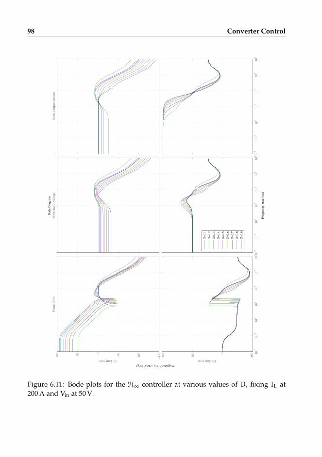
98 Converter Control
Bo
de
Dia
gra
m
Fre
qu
ency
(ra
d/
sec)
Magnitude (dB) ; Phase (deg)
10−
410
−2
100
102
104
106
108
10−
410
−2
100
102
104
106
108
10−
410
−2
100
102
104
106
108
−18
00
180
360
To: Duty ratio
Fro
m: O
utp
ut
curr
ent
Fro
m: I
np
ut
vo
ltag
e
−15
0
−10
0
−50
0
50
100
Fro
m: E
rro
r
To: Duty ratio
D=
0.1
D=
0.2
D=
0.3
D=
0.4
D=
0.5
D=
0.6
D=
0.7
D=
0.8
D=
0.9
Figure 6.11: Bode plots for the H∞ controller at various values of D, fixing IL at200 A and Vin at 50 V.

6.5. Pulse-Width Modulation: H∞ Linear Control 99
The optimisation algorithm’s reason for this is to dampen the system’s naturalfrequency in the feedback loop.
• At high frequencies, all transfer functions are subject to two left-hand-planepoles, whose locations on the frequency axis seems to be roughly coincidentand constant at high frequencies, with some dependence on D and the IL
Vinratio.
• Input voltage signal vin is subject to a left-hand-plane zero occurring at fre-quencies lower than the two poles. Its position is influenced mainly by the IL
Vinratio.
• Interestingly, the optimisation algorithm places a RHP zero on the output cur-rent’s signal, which will cause an inverse response to appear in the controller.Its location on the frequency axis seems to be influenced chiefly byD and IL
Vin.
• The gain for the error signal seems not to be influenced by IL. At low fre-quencies, the large steady-state gain may indicate the opportunity of addingan integrator instead of a pole (an H∞ synthesis algorithm cannot add an in-tegrator by itself, as its H∞ norm is infinite).
• The steady-state gain for channel vin increases with D and decreases with IL.
• The steady-state gain for iout, instead, decreases with both D and Vin.
The step responses of vC and d for various values of IL and Vin, at constant Dand location of zRHP, are presented in figure 6.12. Other step responses for other con-ditions are presented in appendix B. From these plots, the following observationscan be made:
• Low values of D tend to induce oscillations in the responses, especially theresponse to steps in reference.
• Steps in reference have very similar responses in vC when the plant’s RHP
zero andD are constant (figure 6.12), confirming the RHP zero’s importance insetting the control performance’s limits. Furthermore, all plots indicate thatthere is an inverse response to a step in reference, however small; this is be-cause feedback cannot eliminate RHP zeroes.
In conclusion, whereas some patterns have been identified in how optimal H∞controllers vary as a function of the chosen linearisation point, too many controllerparameters change as a function of this point, and they do not suggest a simple and

100 Converter Control
Ste
p R
esp
on
se
Tim
e (s
ec)
Amplitude
00.
005
0.01
0.01
50.
020.
025
0.03
0.03
50.
040.
045
Fro
m: R
efer
ence
sig
nal
00.
005
0.01
0.01
50.
020.
025
0.03
0.03
50.
040.
045
Fro
m: O
utp
ut
curr
ent
00.
005
0.01
0.01
50.
020.
025
0.03
0.03
50.
040.
045
−3
−2
−10123
To: Duty ratio−0.
50
0.51
1.5
Fro
m: I
np
ut
vo
ltag
e
To: Error
IL=
20 A
, Vin
=20
V
IL=
40 A
, Vin
=40
V
IL=
60 A
, Vin
=60
V
IL=
80 A
, Vin
=80
V
IL=
100
A, V
in=
100
V
IL=
120
A, V
in=
120
V
IL=
140
A, V
in=
140
V
IL=
160
A, V
in=
160
V
IL=
180
A, V
in=
180
V
IL=
200
A, V
in=
200
V
Figure 6.12: Step responses for the closed H∞-controlled system at various valuesof IL and Vin, fixing D at 0.5 and the ratio IL
Vinat 1 A/V.

6.6. Pulse-Width Modulation: Feedforward Control 101
Figure 6.13: Feedforward control by filtering of input D.
obvious strategy to find a “good”, almost H∞-optimal controller when a linearisa-tion point is given. A gain-scheduling approach would then have to implement a(possibly cumbersome) set of pre-calculated H∞ controllers for all expected areasof operation.
6.6 Pulse-Width Modulation: Feedforward Control
If the converter is going to be used as an actuator in a larger feedback control loop, asimple control strategy for the inner loop is not to have any feedback control, and letthe external feedback loop take care of disturbance rejection and precise referencetracking.
The simplest strategy to set the output voltage is to measure Vin and set D ac-cording to the steady-state equation:
D =VrefC
VrefC + Vin
(6.23)
However, the system’s oscillations will take some time to decay. One alternativeis adding a lag element, but this will reduce the converter’s dynamic performance5.
5Strictly speaking, left-hand plane poles do not pose fundamental limitations to control perfor-mance, but in this case the manipulable variable has a range of values limited to [0, 1].

102 Converter Control
6.6.1 Half-Delay Filtering
We will consider the possibility of reducing oscillations by filtering the manipulatedvariable’s signal in such a way as to minimise the oscillations induced by it. The ideais to split the signal of manipulated variable D in two parts, so that the second partcounteracts the oscillations caused by the first.
Referring to figure 6.13, we consider a system at steady state withD = D0. Whena step fromD0 toD1 is required by the reference signal,D is set to a “halfway” valueD1/2 for a time π
√LC
1−D1/2, exactly half the oscillation period, after which it is set to its
final value D1.This input filter can be implemented with a partial delay: a fraction of the signal
is delayed by a variable time (half the period of oscillations at D = D1/2), while theother part is immediately sent to the output. The value ofD1/2 can be approximatedby (D0 + D1)/2, but this will cause some residual oscillations when the distancebetween D0 and D1 is large. To obtain a more precise value, we first notice fromfigure 6.13 that the inductor current associated to duty ratio D1/2 has to be halfwaybetween IL(D0) and IL(D1). Therefore:
IL(D1/2) = Iout1
1 −D1/2=IL(D0) + IL(D1)
2=Iout
2
(1
1 −D0+
11 −D1
)(6.24)
It follows than D1/2 can be calculated from D0 and D1 with the relationship:
11 −D1/2
=12
(1
1 −D0+
11 −D1
)(6.25)
The resulting input filter is shown in figure 6.14. Given a reference VrefC , the value
of (1 −D1)−1 is calculated. The signal is then split in two parts, one going directly
to the output and one passing through a delay. After addition, the resulting signalis converted from (1 −D)−1 intoD. The time delay varies depending on the currentvalue of the output.
A series of steps in the reference signal for output voltage has been simulatedin figure 6.15. Input filtering significantly reduces the oscillations associated withthe steps in reference. However, since the steady-state points are not located on astraight line (as simplified in figure 6.9 and 6.13), some oscillations remain. It hasbeen found that adding a low-pass filter with time constant τ =
√LC reduces these
remaining oscillations, at the price of an only slight reduction in rise time (see line“Half delay, low pass” in figure 6.15).
The main drawbacks of this half-delay strategy are its sensitivity to variationsin external current and the loss in phase caused by the delay. Since the half-delay

6.6. Pulse-Width Modulation: Feedforward Control 103
Vin
V refC // f
(VC+VinVin
) 11−D1 // 1
2//
+ e
−π√LC
1−D +// // f
( 11−D
)D //
OO
Figure 6.14: The half-delay input filter. The f() elements represent nonlinearities.
0
20
40
60
80
100
120
140
160
0 0.1 0.2 0.3 0.4 0.5 0.6 0.7
Ou
tpu
t v
olt
age,
V
Time, s
Reference
No input filtering
Half delay
Half delay, low-pass
Figure 6.15: Simulation of a series of steps with feedforward control. No modellingerror or disturbances are considered, and the external current is assumed constantat 20 A.

104 Converter Control
-50
0
50
100
150
200
0 0.5 1 1.5 2 2.5 3 3.5 4
Ou
tpu
t v
olt
age,
V
Time, s
Reference (80 V)
Output voltage
Figure 6.16: The oscillations induced by a step in external current, from 20 to 80 A,on a converter controlled by feedforward half-delay input filtering, with a set pointof 80 V.
filter neither measures the external current nor has any internal form of feedback,variations in external current will induce oscillations that will be dampened onlyby the internal losses, as pictured in figure 6.16. The loss in phase caused by thepresence of a delay in the filter may reduce the achievable performance when anexternal controller is designed using the converter as an actuator.
6.7 Pulse-Width Modulation: Input-Output Linearisation
In order to translate the nonlinear dynamics of buck-boost converters into a moremanageable form, we will try to apply input-output linearisation to this problem.Input-output linearisation is a technique in which a system’s variables are changedso that the system becomes linear in the transformed variables, and the problembecomes treatable by means of linear analysis and synthesis. The general theory ispresented in most books about nonlinear control, such as Slotine and Li [16].
The nonlinear model of a buck-boost converter controlled by pulse-width mod-ulation (6.8) is in the particular form x = f(x)+g(x)D, known as the companion form.This particular form allows the use of some common methods for input-output lin-earisation.

6.7. Pulse-Width Modulation: Input-Output Linearisation 105
6.7.1 Change of Variables
We will adopt the following notation for the linearised system:
• µ is the linearised system’s controlled variable;
• ν is the manipulated variable;
• ψ represents the internal (hidden) dynamics, independent from the manipu-lated variable ν and upon which µ does not depend.
Since we are interested in controlling VC, it is trivial to set:
µ = VC (6.26)
ν can then be chosen as:
ν =IL (1 −D) − Iout
C(6.27)
The rest of the model will be translated into the choice of variable ψ. In order toenforce the hypothesis that ψ does not depend on the manipulated variable, the Liederivative of ψ along the direction identified by g(x) must be zero6. This amountsto:
∇ψ · g(x) =
[∂ψ∂IL∂ψ∂VC
]·[VC+VinL
−ILC
]= 0 (6.28)
This problem accepts the following solution:
ψ =12L I2L +
12C (VC + Vin)2 (6.29)
However, with this choice we lose information on the sign of IL, which maychange in some transients. For conversion purposes, we set ξ = sgn(IL). The pointsidentified by a certain value of ψ in the VC-IL plane are illustrated in figure 6.17.The inverse transformation of equations 6.26 and 6.29 is:
VC = µ
IL = ξ
√2ψ− C (µ+ Vin)2
L
(6.30)
Since∇ψ · g(x) = 0 by construction, the differential equation for ψ can be foundby the relation:
6In other words, ψmust be such that ν cannot bring the system towards different values of ψ.

106 Converter Control
Figure 6.17: The ellipses describing the values of ψ in the VC-IL plane. Functiong(x) is always tangent to the ellipses, and varying ν will not cause the operatingpoint to move to a different value of ψ.
ψ = ∇ψ · x , ∇ψ · f(x)
= −VC IL + (VC + Vin) (IL − Ia)
= Vin IL − (µ+ Vin) Ia
(6.31)
The resulting system of differential equations expressed in the linearised vari-ables is therefore:
ψ = Vin ξ
√2ψ− C (µ+ Vin)2
L− (µ+ Vin) Iout
µ = ν
(6.32)
Only the second equation is actually linear, but it is also the only one that isof interest: ψ has no direct influence on the evolution of µ7, which we can controlby setting ν. However, before we decide to ignore ψ, we must check whether it isstable.
7This is not entirely true, since D is limited between 0 and 1: this means that ν will also be limitedbetween −Iout/C and (IL − Iout)/C, the latter bound ultimately depending on ψ.

6.7. Pulse-Width Modulation: Input-Output Linearisation 107
6.7.2 Internal Dynamics
Unfortunately, the internal dynamics of the linearised system 6.32 is not stable.Naming ψ = w(µ,ψ), we have:
∂w(ψ,µ)
∂ψ=
Vin ξ
L
√2ψ−C (µ+Vin)2
L
=Vin
L IL> 0 for IL > 0 (6.33)
The cause of this instability is the fact that, whenψ is increased at constant µ, thetransient that is begun will bring the operating point to higher values of ψ. In theoriginal system, a step in the input would have caused a spiral-shaped transient thatwould have eventually settled into the steady-state point; in the linearised system,since we use ν instead of D as a manipulated variable, we can easily control µ, butψ is left to itself. Since ν depends on IL, another possible interpretation is that wehave introduced a destabilising feedback loop.
We can illustrate this problem and what it implies in the case of fuel cells byapplying a simple proportional feedback controller in the form ν = Kc (Vref
C − µ) toa converter connected to a fuel-cell stack. Assuming that measurements on IL andIout are free of noise, bias or delay, µwill be stabilised around Vref
C for every Kc > 0.However, according to equation 6.33, ψ will become unstable. When connected toa fuel cell, two scenarios are possible:
1. ψ falls to lower values, and stops only when IL reaches the value of Iout. Atthis point, because of how νwas defined (6.27), µ = ν > 0 would implyD < 0,which is beyond input saturation; D is left to zero as long as Vref
C > µ.
2. ψ rises to higher values, and stops only when IL reaches the fuel cell’s mass-transport limit and the stack produces almost no voltage. The converter willbe able to deliver the required power, but the stack will be operating in ahighly inefficient regime because of the high losses associated with operationat the mass-transport limit. Because of the low stack voltage, D will be veryclose to 1 in order to provide a much higher voltage to the converter output.
These two kinds of failure are illustrated in figure 6.18 and 6.19, using Kc =
100 Hz for the proportional controller. In this figure, two identical, consecutive se-ries of steps in reference from 0 to 200 V and back are simulated. In the first cycle,ψ’s instability makes it fall to lower values, and eventually results in D being setto zero (some residual oscillations can be observed from that point). The currentthrough the fuel cell falls to zero and stack voltage tends to its open-circuit value.
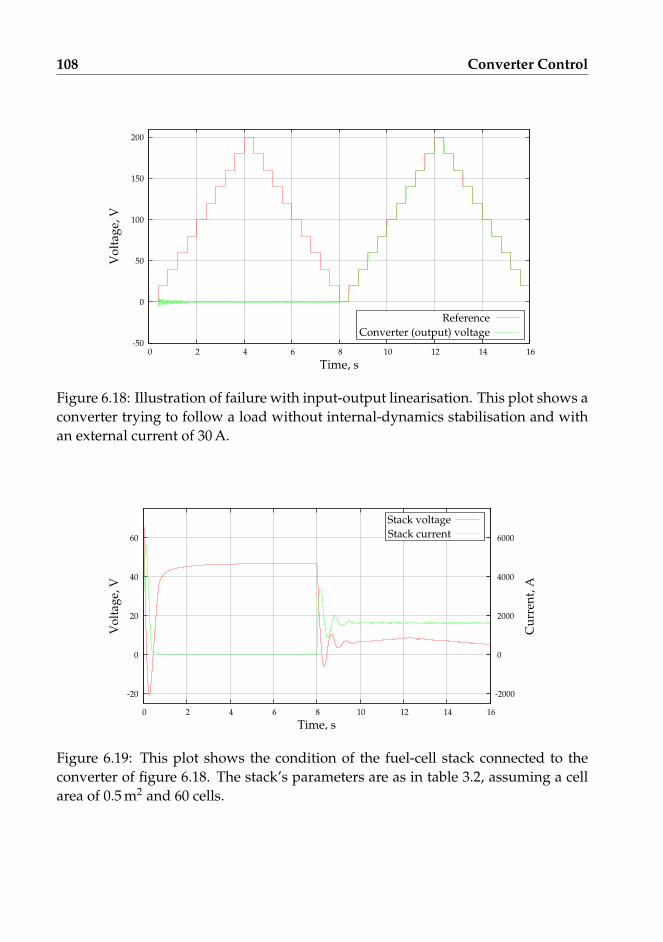
108 Converter Control
-50
0
50
100
150
200
0 2 4 6 8 10 12 14 16
Vo
ltag
e, V
Time, s
Reference
Converter (output) voltage
Figure 6.18: Illustration of failure with input-output linearisation. This plot shows aconverter trying to follow a load without internal-dynamics stabilisation and withan external current of 30 A.
-20
0
20
40
60
0 2 4 6 8 10 12 14 16
-2000
0
2000
4000
6000
Vo
ltag
e, V
Cu
rren
t, A
Time, s
Stack voltage
Stack current
Figure 6.19: This plot shows the condition of the fuel-cell stack connected to theconverter of figure 6.18. The stack’s parameters are as in table 3.2, assuming a cellarea of 0.5 m2 and 60 cells.

6.7. Pulse-Width Modulation: Input-Output Linearisation 109
When the reference returns to zero, D is “unlocked” as ψ falls, this time, on theside of higher values. Tracking proves to be excellent8, yet, as figure 6.19 shows, thestack’s voltage and current indicate that the stack is operating at the mass-transportlimit: at times when higher power is required by the converter, the stack voltagegoes up to match the power demand: we would expect it to go down because ofincreased reactant consumption.
Whereas a fuel-cell stack may deliver power through a converter in these condi-tions, it is hardly an efficient way: in particular, this layout features maximum con-sumption at zero power delivery, all power being used to overcome the diffusion-induced overvoltage.
It should be remarked that there is an important role of numerical noise in de-termining whether ψwill go to the side of high or low values. Figures 6.18 and 6.19could therefore not be exactly reproduced when simulated with slightly differentparameters or even just on different operating systems.
In fact, this approach could in principle not have worked as originally intended,as controlling an integrator process with proportional feedback allows perfect con-trol when the proportionality constant of the controller tends to infinity, but perfectcontrol is theoretically impossible in non-minimum-phase systems. This exampleclearly indicates the need to stabilise the internal dynamics of the linearised systemin order to properly control the reaction rate in the fuel cell.
6.7.3 Stabilisation of the Internal Dynamics
Stabilising the internal dynamics of non-minimum-phase nonlinear systems is anactive field of current research, and there are no general methods to guarantee cer-tain performance requirements on feedback control. In general, however, stabilisingthe internal dynamics means to constrain µ to be a function of ψ so that the totalderivative of w(ψ,µ) is kept negative:
dw(ψ,µ)
dψ=∂w(ψ,µ)
∂ψ+∂w(ψ,µ)
∂µ
dµdψ
< 0 (6.34)
Enforcing this condition will reduce oscillations in the VC-IL phase plane, astrajectories close to the steady-state value of ψ will be attracted by it. If the con-trol algorithm ν(µ,ψ) can be chosen so that dν
dµ < 0 as well, oscillations will beeliminated as both state variables will converge to the steady state.
Since the second partial-derivative term in equation 6.34 is:
8To be fair, we did not model any error in calculations or measurement, so perfect control could beobtained just by applying an infinite gain.

110 Converter Control
∂w(ψ,µ)
∂µ= −
C (µ+ Vin)Vin ξ
L
√2ψ−C (µ+Vin)2
L
− Iout = −C (µ+ Vin)Vin
L IL− Iout (6.35)
We can reformulate condition 6.34 as:
Vin
L IL−
(C(µ+ Vin)Vin
L IL+ Iout
)dµdψ
< 0 (6.36)
Manipulating this expression, the condition on the dependence of µ from ψ be-comes:
dµdψ
>Vin
C (µ+ Vin)Vin + L IL Iout(6.37)
However, µ is determined by ν in the linearised system 6.32. As ν is our manip-ulated variable, it makes sense to translate this condition in terms of ν:
ν = µ =dµdψ
ψ (6.38)
ν sgn(ψ) >Vin |ψ|
C (µ+ Vin)Vin + L IL Iout(6.39)
We have therefore translated the stabilisation ofψ into a requirement on the val-ues that ν can have. At steady state there is no requirement, as ψ = 0 by definitionof steady state. During transients, ν must have the same sign as ψ and must belarger, in absolute value, than a certain lower limit.
6.7.4 Feedback with Input Bounds
Having obtained a bound on ν as a function of measurable quantities (the inputand output currents and voltages), it seems natural to devise a simple feedbackcontrol law for µ (possibly a high-gain proportional controller) and filter the inputν through bound 6.39, to avoid instability. However, this approach runs rapidlyinto problems.
When a simulation is started from a non-steady-state point, the bound on νforces the operating point to µ = 0, IL = Iout; oscillations are induced by the satura-tion constraint D ∈ [0, 1], which the required bound on ν tries to violate. Transientsend invariably with the controller requiring D < 0, with the fuel cell being cut offfrom the converter.

6.7. Pulse-Width Modulation: Input-Output Linearisation 111
The reason for this failure can ultimately be traced to the fact that this systemcannot completely eliminate oscillations, as observed by means of linear controlla-bility analysis in section 6.5.1: if condition 6.39 could be enforced strictly, we wouldhave achieved what it was already demonstrated to be impossible.
6.7.5 Feedforward with Internal Oscillation Dampening
As feedback proved problematic with this non-minimum-phase nonlinear system,another approach was attempted: on one hand, an unfiltered valueD0 is calculatedfrom reference Vref
C and the measurement Vin, as in equation 6.23. This is used tocompute a corresponding ν0 with equation 6.27. Then, this value is added to a νψ,obtained from bound 6.39, that has the function of dampening the oscillations:
νψ =Vin ψ
C (µ+ Vin)Vin + L IL Iout(6.40)
The final D passed to the converter is then obtained inverting equation 6.27 forν = νD + νψ. Since the conversion function is linear in ν, it is possible to separatethe two terms:
D = 1 −Iout + C (ν0 + νψ)
IL= D0 − C
νψ
IL(6.41)
This approach allows for a certain amount of oscillations, since the final ν isnot strictly bounded by equation 6.39, which acts here as a dampening element.Performance is not very good with very low values of Iout, where dynamics areslower. Operation at low values of Iout is however inherently difficult with anyapproach, as Iout is the only term that can reduce the value of VC in its differentialequation.
A series of steps in reference is shown in figure 6.20, where it can be seen thattransients at the highest voltages are somewhat slower, as should be expected fromequation 6.14, which expresses that a converter’s natural oscillation frequency islower for high values of D; overall performance is however satisfactory, and thefuel-cell stack does not operate at the mass-transport barrier, but at lower currents,yielding higher efficiency. As this is a feedforward technique, there is some steady-state offset caused by losses in the converter, which may be evened out by an ex-ternal feedback loop that could use the converter as an actuator. Oscillation damp-ening is excellent, as shown in figure 6.21: compared to figure 6.16, the transient isshortened by two orders of magnitude.
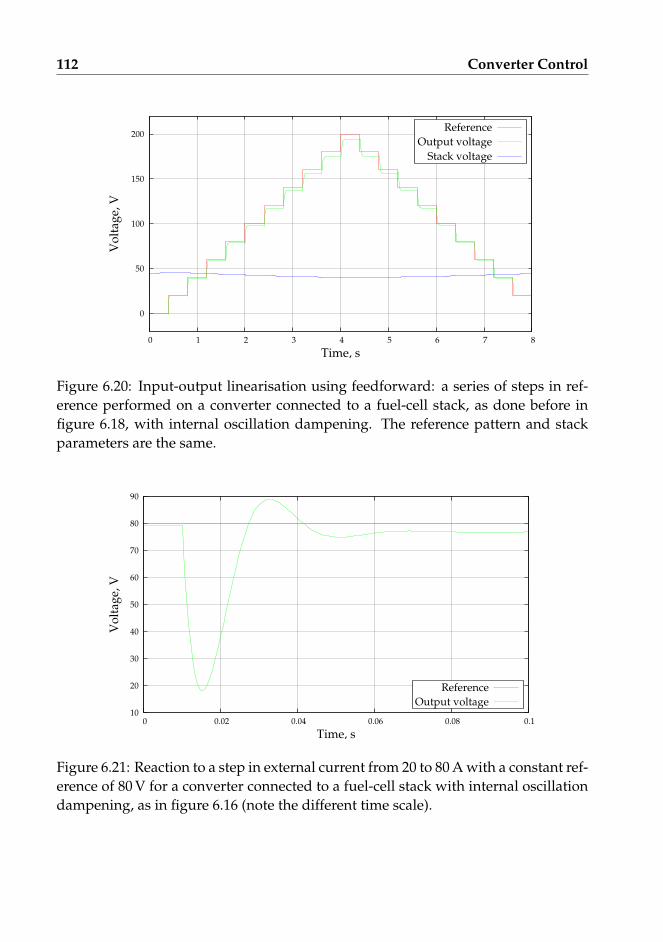
112 Converter Control
0
50
100
150
200
0 1 2 3 4 5 6 7 8
Vo
ltag
e, V
Time, s
Reference
Output voltage
Stack voltage
Figure 6.20: Input-output linearisation using feedforward: a series of steps in ref-erence performed on a converter connected to a fuel-cell stack, as done before infigure 6.18, with internal oscillation dampening. The reference pattern and stackparameters are the same.
10
20
30
40
50
60
70
80
90
0 0.02 0.04 0.06 0.08 0.1
Vo
ltag
e, V
Time, s
Reference
Output voltage
Figure 6.21: Reaction to a step in external current from 20 to 80 A with a constant ref-erence of 80 V for a converter connected to a fuel-cell stack with internal oscillationdampening, as in figure 6.16 (note the different time scale).

6.8. Switching Rules 113
6.8 Switching Rules
We will now attempt a different approach to the problem of controlling a buck-boostconverter. We will try to devise a set of logical rules to determine when the switchshould be in the ON or OFF position, instead of using the duty ratio as a continuousinput variable.
This section will try an approach similar to sliding-mode control by definingsome switching rules. Instead of the usual constant sliding surfaces as described bySpiazzi and Mattavelli [2], a series of variable surfaces were devised to take advan-tage of the shape of trajectories of the system in the VC-IL plane. This is helpful,as their shape can change considerably depending on external disturbances (suchas Iout and Vin), which represent the effect of having a variable voltage source andan unknown load. This is strictly speaking not sliding-mode control, as in fact noone of the defined surfaces will actually be a sliding mode. The rules, however, domake sure that the desired output is attained.
The equations describing our system are, when the fuel-cell stack is connectedto the inductor (the ON position in figure 6.4):
Ld ILd t
= Vin
CdVCd t
= −Iout
(6.42)
Vin and Iout are considered to be external entities with respect to the converter,and are assumed to maintain a positive sign. The trajectories described by theseequations are straight lines, since Iout and Vin are assumed not to depend directlyon IL or VC.
When the switch is positioned so that the inductor is connected to the capacitor(the OFF position in figure 6.4), the equations are instead:
Ld ILd t
= −VC
CdVCd t
= IL − Iout
(6.43)
The trajectories described by these equations are a series of ellipses, centered atthe point (0, Iout), whose parametric equation can be given as:
12L (IL − Iout)
2 +12CV2
C = c c ∈ R+0 (6.44)
Obviously, if Iout were to change during the transient, the centre of the ellipseswould move and the actual trajectory of a point could not resemble an ellipse at all.

114 Converter Control
Figure 6.22: The trajectories of the state variables in a buck-boost converter in theVC-IL plane for given values of external disturbances Vin, Iout.
It would be tempting to define these curves as representatives of the amount ofenergy physically stored in the converter, but the first term in equation 6.44 is notthe energy stored in the inductor’s magnetic field. The value of c, however, canindeed be mathematically interpreted as representative of the system’s energy, ifnot physically.
The trajectories corresponding to these equations are shown in figure 6.22. TheON mode is represented on the left-hand side, where energy is collected from theinput by the inductor. On the right-hand side (the OFF mode), no energy is drawnfrom the source, and the energy stored in the inductor is exchanged with the capaci-tor. The capacitor exchanges power with the output in both configurations. In a realsystem, the trajectories on the right-hand side would be spirals, because of losses inthe switches.
6.8.1 Control Rules
The objective of the switching rules is to maintain a certain value of the converter’soutput voltage by switching the system between its two substructures, as shownin figures 6.4 and 6.22, accounting for the changes in output current, caused by theload, and in input voltage, caused by the fuel-cell stack. The rules will have to becalculated at each iteration, using new measurements for Vin, IL, VC and Iout, andare formulated as follows:
Energy level If the value of c in equation 6.44 is not sufficiently high, the ellipticaltrajectories of the OFF mode will not be able to reach Vref
C . Therefore, the onlypossibility left is to switch to the linear trajectories of the ON mode until asufficiently high energy level is reached. It will then be possible to switch to

6.8. Switching Rules 115
the OFF mode and reach VrefC .
The “sufficiently high” energy level is however not the one correspondingto an ellipse of the OFF mode that has its extreme point in Vref
C . If it wereso, it would not be possible to maintain the operating point at that value byswitching back to the ON mode: the ON mode, which in general has a non-zero component along the VC axis, would cause the system to fall to a lowerenergy level, at which it should maintain the ON state until reaching again ahigh enough energy level. An hysteresis cycle would then result, which wouldyield an unsatisfactory performance.
The correct energy level is therefore the one corresponding to the ellipse that,at the reference voltage Vref
C , is tangent to the lines of the ON mode. The un-avoidable imprecision in parameter estimation and measurement will causesome oscillation, however.
The mathematical formulation of the rule is:
12CV2
C +12L (IL − Iout)
2<
12CVref
C
2+
12L
(VrefC Iout
Vin
)2
⇒ ON (6.45)
High-voltage switch At voltages higher that VrefC , the surface at which one moves
from one substructure to the other is given by the tangent line departing fromthe ellipse described above at voltage Vref
C . Since this line is by constructionparallel to the lines of the ON mode, once the operating point crosses thisline arriving from an elliptical trajectory of the OFF mode, it is not possiblefor it to return back. This is important because there is no guarantee thatthe component of the ON-mode derivatives along a given line are larger thanthe OFF-mode’s, because the former are disturbances that we do not directlycontrol.
The mathematical formulation of the rule is:
VC > VrefC ∧ IL − Iout <
VrefC Iout
Vin−C
L
Vin
Iout
(VC − Vref
C
)⇒ ON (6.46)
Low-voltage switch It is not unlikely that, during transients, voltage VC will reachnegative values. In fact, it is quite a common phenomenon in transients, evenif it lasts only for a short time. A reasonable control objective is to minimisethe inverse response during such a transient. Therefore, if during a transientVC is less than zero, and the energy level is sufficient as defined above, the
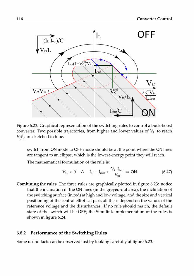
116 Converter Control
Figure 6.23: Graphical representation of the switching rules to control a buck-boostconverter. Two possible trajectories, from higher and lower values of VC to reachVrefC , are sketched in blue.
switch from ON mode to OFF mode should be at the point where the ON linesare tangent to an ellipse, which is the lowest-energy point they will reach.
The mathematical formulation of the rule is:
VC < 0 ∧ IL − Iout <VC Iout
Vin⇒ ON (6.47)
Combining the rules The three rules are graphically plotted in figure 6.23: noticethat the inclination of the ON lines (in the greyed-out area), the inclination ofthe switching surface (in red) at high and low voltage, and the size and verticalpositioning of the central elliptical part, all these depend on the values of thereference voltage and the disturbances. If no rule should match, the defaultstate of the switch will be OFF; the Simulink implementation of the rules isshown in figure 6.24.
6.8.2 Performance of the Switching Rules
Some useful facts can be observed just by looking carefully at figure 6.23.

6.8. Switching Rules 117
1
Vc
ZOH
Ia
Vw
Vc
iL
Slide!
Low−voltageslide
VrefIaVwVciL
Low energy
Low energy?
OR
VrefIaVwVciL
Slide!
High−voltageslide
D
Ia
Vc
iL
Vw
Converter(physical system)
2
Ia
1
Vref
D
Figure 6.24: The Simulink implementation of the switching rules. The rules’ resultis passed through a zero-order hold element (ZOH), whose time parameter sets theswitching frequency. The zero-order hold’s output is then passed to a block mod-elling the converter.
• Steps in VrefC will in general exhibit an inverse response. When Vref
C has toincrease, the operating point has to accumulate enough energy along the ON-mode lines, which will cause an initial reduction of VC. When Vref
C has todecrease, the operating point first follows the OFF-mode elliptical trajectoriesuntil it reaches either their maximum value of voltage, or the switching surfacedescribed by rule 6.46, before decreasing again.
• Steps in Iout will have a similar effect, but this is intuitive: more current atthe output, at the same output voltage, means more power delivered, and theconverter will have to gradually adapt to this new regime.
• The set of rules does not permit to specify a negative VrefC . This is intentional,
because, with a positive Iout, power would be drawn from the outer circuit tothe fuel cell, causing reverse electrolysis, and likely damaging the fuel cell’scatalyst.
A simulated transient is shown in figure 6.25. It can be noticed how the inverseresponse is much more significant at high values of Iout. The transients have fast set-tling times, about 5 ms: this is faster than the 0.2 s required for vehicles (accordingto Soroush and Elabd [17]), and can make this control strategy useful also for mi-croelectronic applications such as laptops and mobile phones. It can also be noticedhow the output becomes more noisy at high values of Iout.
A problem may arise when the converter is required to produce exactly 0 volts,even if Iout is larger than 0. The converter’s switching rules degenerate in a special

118 Converter Control
-150
-100
-50
0
50
100
150
200
250
0 0.01 0.02 0.03 0.04 0.05-150
-100
-50
0
50
100
150
200
250V
olt
age,
V
Cu
rren
t, A
Time, s
Reference voltage
Output voltage
Output current
Figure 6.25: Simulated transient of a buck-boost converter, controlled with switch-ing rules. The switching frequency has been set to 10 µs.
Figure 6.26: The approximate trajectory of the operating point when VrefC = 0 and
Iout = 0. Higher switching frequencies will shrink the trajectory towards the origin.

6.8. Switching Rules 119
case: output voltage oscillates around the origin in an asymmetrical fashion, assketched in figure 6.26, resulting in a net average positive value of VC and possiblywind-up issues in the outer control loop. While the amplitude of such oscillationscan be reduced with a higher switching frequency, their average value will alwaysbe positive.
To address this issue, a new simple rule for the converter can be added:
VrefC 6 0 ⇒ OFF (6.48)
It is important to notice that rule 6.48 takes precedence on all others, since it mightbe contradicting them. The meaning of this rule is that the fuel-cell stack must bedisconnected whenever there is an unachievably low objective. In an actual appli-cation, the voltage will then gradually decrease to zero because of dissipation inexternal load and in the converter switches.
6.8.3 Computational Performance
The simulation times of this controller are relatively long; the transient in figure 6.25requires about 50 seconds to calculate on a 2-GHz, 32-bit desktop computer runningSimulink. This makes simulation over longer time spans unpractical. The fuel cell’sovervoltage, when starting the simulation, needs some time to reach a steady-statevalue from zero, and this initialisation transient may interfere with the transientswe are interested in measuring. In practice, using this method to study how thefuel cell reacts to control is not computationally convenient.
The main reason for such an unsatisfactory computational efficiency is that therules are evaluated every 10 µs (in the case of figure 6.25), and a transient has tobe calculated every time the algorithm requires a switch. When the transients set-tle9, the manipulated variable does not attain a constant value, but is continuouslyswitched between ON and OFF. Integration algorithms for stiff systems do not pro-vide any sensible improvement.
Implementing this control algorithm would likely imply building a dedicatedcircuit to simulate the switching rules, which only require basic arithmetic and log-ical operations: indeed, the actual determination of whether the switch should beON or OFF is a small part of the computational cost. However, the numerical sim-ulation of the converter’s transients with this control strategy is computationallyvery expensive, as every switching cycle implies a sudden change in the model’sequations.
9In reality, only macroscopic transients settle, because the control algorithm is in fact based onrapidly switching between two transients compensating each other.

120 Converter Control
Using the model based on pulse-width modulation, which uses a continuousmanipulated variable, improves the simulation performance, even though the con-trol performance is inferior because of the additional level of abstraction.
6.9 Conclusions
Some insight about control of fuel-cell power output can be obtained from the var-ious approaches analysed in this chapter. The main control issue are the nonlinear,non-minimum-phase dynamics of the buck-boost converter.
Controlling DC motors, a likely appliance for fuel-cell power generation, is usu-ally done by manipulating the input voltage to the motor. Therefore, the controlproblem for the converter was defined as to deliver a certain output voltage in spiteof external disturbances, such as input voltage (changing because of variations inthe stack voltage) and output current (changing because of variations in motor con-ditions, such as angular velocity).
First, a model based on pulse-width modulation was presented. A local lineari-sation around a generic steady state was performed to attempt an H∞ controllersynthesis. The manipulated input (the duty ratio) was proven to be subject to aRHP zero, which is strongly dependent on the linearisation point: this poses inher-ent limitations to control performance. Disturbance rejection is influenced by theposition of the RHP zero, but also by the duty ratio at the linearisation point.
A simple feedforward control strategy has then been attempted, resulting ingood tracking qualities. However, this approach resulted in high sensitivity to dis-turbances because of the low power dissipation in the converter. Input-output lin-earisation was then attempted, proving that the model of the system with pulse-width modulation is non-minimum-phase in the nonlinear sense as well, and re-quires some sort of stabilisation of the internal dynamics. A feedforward approachcoupled with an oscillation-dampening component (in itself a form of feedback)gave satisfactory results in both tracking and oscillation dampening.
Finally, a method based on the evaluation of switching rules has been proposed,and has yielded very good results, with settling times of about 5 ms. This methodmay in practice be realised with relatively simple hardware, as it does not implymore than a few arithmetic and logical operations. However, it is more difficult torigorously evaluate the robustness of this method to uncertain or lagging measure-ments. This method also unsuitable for computer simulations beyond the scale of afew seconds: this means it is difficult to simulate a fuel cell’s operation under thistype of control.

Bibliography 121
Bibliography
[1] Michael Giesselmann, Hossein Salehfar, Hamid A. Toliyat, and Tahmid Ur Rahman.The Power Electronics Handbook, chapter 7 - Modulation Strategies. Industrial electron-ics. CRC press, 2001.
[2] Giorgio Spiazzi and Paolo Mattavelli. The Power Electronics Handbook, chapter 8 -Sliding-Mode Control of Switched-Mode Power Supplies. Industrial electronics. CRCpress, 2001.
[3] Jai P. Agrawal. Power Electronic Systems — Theory and Design. Prentice Hall, 2001.
[4] T. Geyer, G. Papafotiou, and M. Morari. On the optimal control of switch-modeDC-DC converters. Hybrid Systems: Computation and Control, 2993:342–356, March2004. URL http://control.ee.ethz.ch/index.cgi?page=publications;action=details;id=31.
[5] Manfred Morari. Beyond process control. In Proceedings of the 13th Nordic Process ControlWorkshop, Lyngby, Denmark, 2006.
[6] Rami Naim, George Weiss, and Shmuel Ben-Yaakov. H∞ control applied to boostpower converters. Transactions on Power Electronics, 12(4):677–683, July 1997.
[7] Fang Lin Luo and Hong Ye. Advanced DC/DC Converters. CRC press, Boca Raton,Florida, USA, 2004.
[8] S. Caux, J. Lachaize, M. Fadel, P. Shott, and L. Nicod. Modelling and control of a fuelcell system and storage elements in transport applications. Journal of Process Control,15:481–491, 2005.
[9] Sébastien E. Gay and Mehrdad Ehsani. Impact of electric motor field-weakening ondrive train oscillations. In Electric Machines and Drives Conference, volume 2, pages641–646, June 2003.
[10] Werner Leonhard. Control of Electrical Drives. Springer, 2nd edition, 2001.
[11] James Larminie and John Lowry. Electric Vehicle Technology Explained. Wiley, 2003.
[12] Chee-Mun Ong. Dynamic Simulation of Electric Machinery. Prentice Hall, 1998.
[13] C. L. Chu, M. C. Tsai, and H. Y. Chen. Torque control of brushless DC motors appliedto electric vehicles. In Electric Machines and Drives Conference, pages 82–87, 2001.
[14] Sigurd Skogestad and Ian Postlethwaite. Multivariable feedback control. Wiley, 2nd edi-tion, 2005.
[15] Karl Johan Åström and Björn Wittenmark. Adaptive Control. Addison Wesley, 1989.

122 Converter Control
[16] Jean-Jacques E. Slotine and Weiping Li. Applied Nonlinear Control. Prentice-Hall, 1991.
[17] Masoud Soroush and Yossef A. Elabd. Process systems engineering challenges in fuelcell technology for automobiles. In AIChE Annual Meeting, 2004.

Chapter 7
Composition and TemperatureControl
Having considered the control of the reaction rate in chapter 6, we turn our attentionto the control of the conditions that allow the reaction to proceed, namely reactantconcentration and stack temperature.
As outlined in chapter 5, we consider a stack of PBI-membrane PEM fuel cells,fed on pure hydrogen on the anodic side and air (possibly after combustion of somehydrogen to heat up the cell) on the cathodic side (such as in figure 5.4 on page 78).
As we are considering a stack of cells whose flows are connected in parallelthrough manifolds, all cells will receive flows at stack-entrance conditions: it istherefore possible to consider only one cell as representative of the conditions ofall the cells in the whole stack. The three main control issues are then:
1. Control of hydrogen pressure in the anode;
2. Control of oxygen bulk concentration in the cathode;
3. Control of temperature in the cell (anode and cathode are assumed to have thesame temperature).
However, for these three tasks we assume that we only have two manipulatedvariables, which are the entering flows of hydrogen on the anode side and air on thecathode side. Thus, the control strategy proposed in this chapter presents the nov-elty of not having a dedicated cooling system to control temperature: temperaturewill be controlled by means of the air flow.
This will however cause a certain degree of interference between the control ofoxygen concentration and that of stack temperature, which both use air flow as their
123
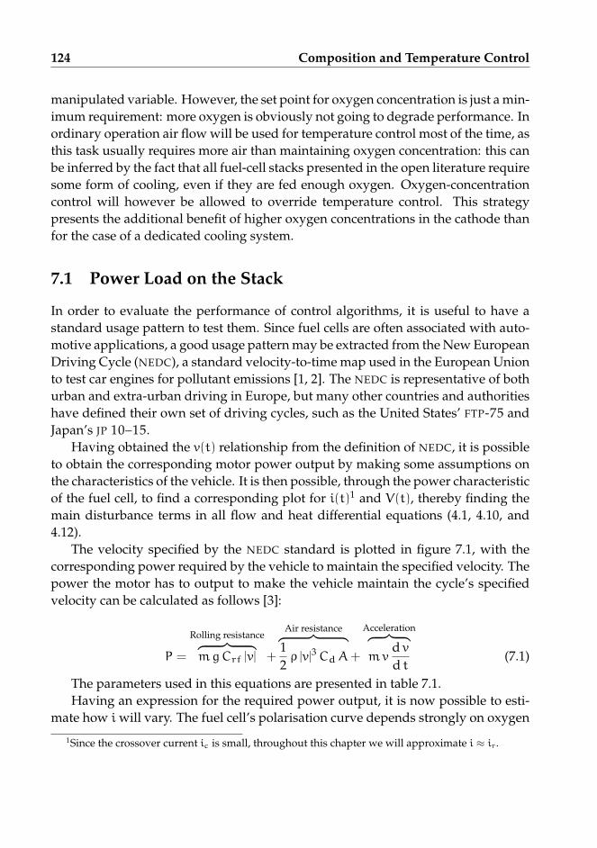
124 Composition and Temperature Control
manipulated variable. However, the set point for oxygen concentration is just a min-imum requirement: more oxygen is obviously not going to degrade performance. Inordinary operation air flow will be used for temperature control most of the time, asthis task usually requires more air than maintaining oxygen concentration: this canbe inferred by the fact that all fuel-cell stacks presented in the open literature requiresome form of cooling, even if they are fed enough oxygen. Oxygen-concentrationcontrol will however be allowed to override temperature control. This strategypresents the additional benefit of higher oxygen concentrations in the cathode thanfor the case of a dedicated cooling system.
7.1 Power Load on the Stack
In order to evaluate the performance of control algorithms, it is useful to have astandard usage pattern to test them. Since fuel cells are often associated with auto-motive applications, a good usage pattern may be extracted from the New EuropeanDriving Cycle (NEDC), a standard velocity-to-time map used in the European Unionto test car engines for pollutant emissions [1, 2]. The NEDC is representative of bothurban and extra-urban driving in Europe, but many other countries and authoritieshave defined their own set of driving cycles, such as the United States’ FTP-75 andJapan’s JP 10–15.
Having obtained the v(t) relationship from the definition of NEDC, it is possibleto obtain the corresponding motor power output by making some assumptions onthe characteristics of the vehicle. It is then possible, through the power characteristicof the fuel cell, to find a corresponding plot for i(t)1 and V(t), thereby finding themain disturbance terms in all flow and heat differential equations (4.1, 4.10, and4.12).
The velocity specified by the NEDC standard is plotted in figure 7.1, with thecorresponding power required by the vehicle to maintain the specified velocity. Thepower the motor has to output to make the vehicle maintain the cycle’s specifiedvelocity can be calculated as follows [3]:
P =
Rolling resistance︷ ︸︸ ︷mgCrf |v| +
Air resistance︷ ︸︸ ︷12ρ |v|3CdA+
Acceleration︷ ︸︸ ︷mv
d vd t
(7.1)
The parameters used in this equations are presented in table 7.1.Having an expression for the required power output, it is now possible to esti-
mate how iwill vary. The fuel cell’s polarisation curve depends strongly on oxygen
1Since the crossover current ic is small, throughout this chapter we will approximate i ≈ ir.
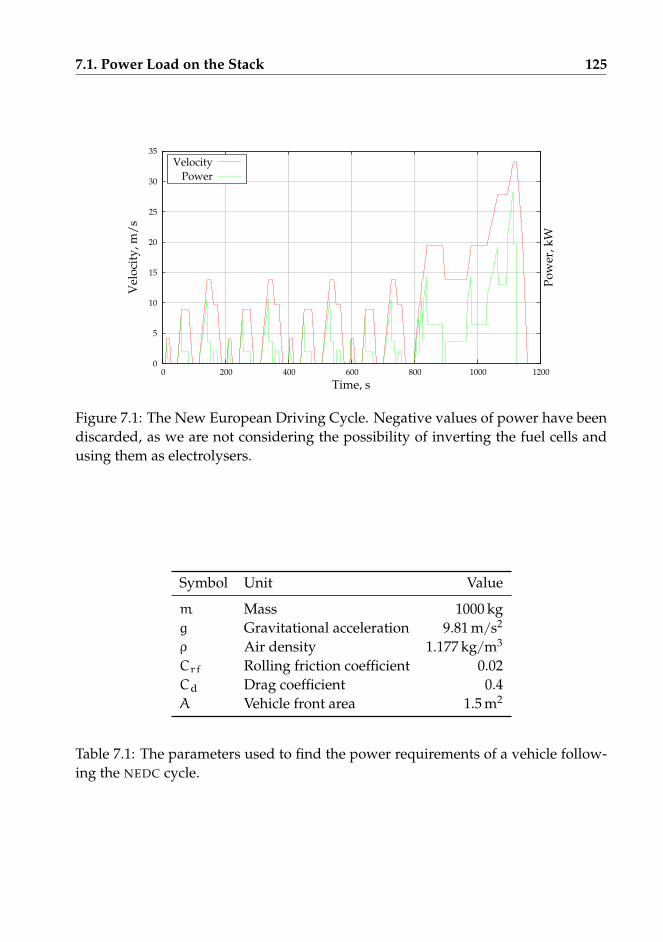
7.1. Power Load on the Stack 125
0
5
10
15
20
25
30
35
0 200 400 600 800 1000 1200
Vel
oci
ty, m
/s
Po
wer
, kW
Time, s
Velocity
Power
Figure 7.1: The New European Driving Cycle. Negative values of power have beendiscarded, as we are not considering the possibility of inverting the fuel cells andusing them as electrolysers.
Symbol Unit Value
m Mass 1000 kgg Gravitational acceleration 9.81 m/s2
ρ Air density 1.177 kg/m3
Crf Rolling friction coefficient 0.02Cd Drag coefficient 0.4A Vehicle front area 1.5 m2
Table 7.1: The parameters used to find the power requirements of a vehicle follow-ing the NEDC cycle.

126 Composition and Temperature Control
0
200
400
600
800
1000
1200
0 500 1000 1500 2000 2500 3000
Po
wer
den
sity
, W/
m2
Current density, A/m2
X = 0.0
X = 0.1
X = 0.2
X = 0.3
X = 0.4
X = 0.5
X = 0.6
X = 0.7
X = 0.8
X = 0.9
Figure 7.2: Effect of conversion on a cell’s power output. The image uses the samedata of figure 4.2.
conversion X in the cathode, as shown in figure 4.2. To invert the relationship P(i,X)
it is therefore first necessary to assume a value for conversion. Figure 4.3 indicatesthat conversion must be low for the highest power outputs to be attainable. Further-more, as shown in figure 7.2, the power output curves do not depend significantlyon X until the mass-transport barrier is actually reached for each curve: each curveseparates from a common envelope when approaching its mass-transport limit. Wewill therefore consider this envelope (X = 0) a representative estimate to invertP(i,X), because we assume that control will be able to keep the stack away from themass-transport limit.
We can now find the rate of oxygen consumption, ir(t)A4F , and heat generation,[∆hr2F − V(t)
]ir(t). In all simulations in the remainder of the chapter, we will as-
sume that the fuel cell stack has a total area of 30 m2, resulting in a theoretical max-imum power output of 31.13 kW, or 9.5 % more than the maximum required powerby NEDC, which is 28.42 kW. Oxygen consumption and heat generation are plottedin figure 7.3, where we can see that they quite closely match the shape of powerrequirement in figure 7.1.
7.2 Pressure Control of Dead-End Flows (Anode)
In the case of dead-end flows, where there is only one reactant and no productsare taken up by the stream, maintaining reactant concentration is equivalent to con-

7.2. Pressure Control of Dead-End Flows (Anode) 127
0
1
2
3
4
5
6
0 200 400 600 800 1000 1200 0
0.5
1
1.5
2
2.5
3
Mo
le C
on
sup
tio
n, m
mo
l/m
2 s
Hea
t G
ener
atio
n, k
W/
m2
Time, s
Oxygen Consumption
Heat Generation
Figure 7.3: The approximate plot of reactant consumption and heat generation alongthe entire NEDC cycle, assuming X = 0. As in practice Xwill be different from 0, realvalues may be slightly higher because of the increased overvoltage.
trolling the gas pressure, assuming negligible temperature variations. In general,but especially in the case of hydrogen coming from a pressurised tank, we wantto avoid excessive pressure difference across the membrane, to reduce mechanicalstress and avoid membrane rupture. As dead-end flows periodically require purg-ing of inert gases, it would be convenient to maintain a pressure slightly higherthan atmospheric: this will have the added benefit of leaking hydrogen out insteadof letting air in, were a leak to occur.
The differential equation we consider is equation 4.3, from which we remove,for simplicity, the term accounting for temperature variation:
dpH2
d t=R T
VnH2
−R T
V
irA
2 F(7.2)
Since the system’s state pH2does not appear in the right-hand term, this is an in-
tegrating process. As integrating processes are not stable, feedback is mandatory: ifthere were no pressure measurement, and we only relied on a current measurementto set the flow to compensate consumption, any error would accumulate over time,and we would eventually either run out of hydrogen or rupture the membrane.
Fortunately, pressure measurements are known to be quick and simple to obtain:Huang and Cheng [4] claim that simple and cheap pressure sensors have responsetimes below 0.5 s. We will model the sensor and actuator lag with a simple delay,θpm = 0.5 s. For this case, Skogestad [5] suggests the following design for a PI

128 Composition and Temperature Control
ir //
//
A2 F
H2 consumption
−
kffA2 F
Feedforward
+pref
H2
+// // Kc
(τI s+1τI s
)+
Feedback// nH2
+// // R T
V1s
pH2//
ooe−θpm
−OO
Figure 7.4: Control diagram for pure hydrogen pressure in a dead-end manifold.
feedback controller:
Kc =V
R T
1τc + θpm
τI = 4 (τc + θpm)
(7.3)
Where the desired response time τc is the tuning parameter, and having definedthe PI control law as:
ufeedback =
K(s)︷ ︸︸ ︷Kc
(τI s+ 1τI s
)(r− y) (7.4)
We can also add some feedforward action, since the only significant disturbancein the process, ir, can be easily and rapidly measured:
ufeedforward = kffirA
2 F(7.5)
Parameter kff is the feedforward implementation error.We are still missing a value for gas volume V. This is the volume downstream
from the control valve that we manipulate to set the molar inflow nH2. As an es-
timate, we assume V = 30 m2 × 1 mm = 30 dm3, where the area is the same weassumed above and 1 mm is the thickness of a gas channel, as reported in Shan and

7.2. Pressure Control of Dead-End Flows (Anode) 129
-100
-50
0
50
100
150
200
250
300
350
0 200 400 600 800 1000 1200
Hy
dro
gen
pre
ssu
re, k
Pa
Time, s
Feedback only
With feedforward, perfect
With feedforward, -20%
With feedforward, +20%
Figure 7.5: The partial pressure of hydrogen as it is controlled by a PI feedbackcontroller, with and without assistance from a feedforward controller (two differentvalues for implementation error are shown), with a set point of 120 kPa, when thefuel cell stack is subject to the NEDC cycle.
Choe [6]. As this estimate neglects the manifold volume, it is expected to be veryconservative. The total gas volume may in fact be increased when designing thestack, to improve control properties by making the dynamics slower and easier todeal with.
To test the performance of this control strategy, we can simulate the effect ofdisturbance ir(t) as calculated previously for an NEDC cycle. We assume a constanttemperature of 150 °C and a set point of p0
H2= 120 kPa, plus the overall loop delay
θpm = 0.5 s.The control system is shown in the control diagram of figure 7.4, with both feed-
forward and feedback control loops, and the simulation results for the NEDC cycleare plotted in figure 7.5. The simulation for the case of feedback-only control indi-cates unsatisfactory performance: in order to cope with integrator wind-up in the PI
controller2, τc was set to a relatively large level, τc = 15 s: larger values would causetoo sluggish control action, whereas lower would result in significant wind-up. Toimprove performance, it was necessary to add feedforward action, also plotted infigure 7.5. Even in the case of large implementation errors (±20 %), feedforwardmakes control performance acceptable. It is however not possible to discard the
2It is possible to set nH2only to values larger than zero, so, if the controller were to require less
than zero values for the manipulated variable, an integrator wind-up may result.
130 Composition and Temperature Control
feedback loop, as system 7.2 is unstable and requires feedback for stabilisation.
7.3 Composition Control of Open-End Flows (Cathode)
Ensuring that oxygen partial pressure in the cathode’s bulk be sufficient is in manyways more challenging than controlling hydrogen pressure. Oxygen’s partial pres-sure is much more critical to the performance of the fuel cell than hydrogen’s, be-cause of the much higher overvoltage on the cathodic side. At the same time, com-position measurements are slower than pressure measurements, resulting in lessavailable bandwidth for feedback control.
The differential equation for the mole fraction of oxygen in a cell’s cathode is aparticular case of equation 4.10:
pV
R T
d xO2
d t= nair
(xin
O2− xO2
)−irA
4 F
(1 + xO2
)(7.6)
This equation presents the additional challenge of being nonlinear, but it has theadvantage, compared to equation 7.2, of being stable: in the right-hand term, thecoefficient of state variable xO2
is strictly negative. This means that feedback is notstrictly necessary, and a pure feedforward approach is possible.
7.3.1 Measurement Dynamics
Measurement of oxygen concentration in gases is frequently reported to be veryfast, with bandwidths in the range of 10 Hz [7], but these are usually papers relatingto measurement of oxygen concentration in off-gases from stacks or car exhausts:these assume temperatures in much higher ranges than the ones we are consider-ing, generally beyond 700 °C: Park et al. [8] published a paper on an oxygen sensorfor “low” temperatures down to 500 °C. Results more relevant for our tempera-ture range (100 to 200 °C) were obtained by Yamamoto et al. [9], who reported thatoxygen sensors operating at 100 °C reached steady state after about three minutes,under various values of composition; their plots indicate that the measurement dy-namics operated roughly as a lag with a time constant of two minutes. These lagsmay be reduced by purpose-built equipment, such as sensors that heat up samplesof the stack’s off-gases to high temperatures to make a faster measurement possible.

7.3. Composition Control of Open-End Flows (Cathode) 131
7.3.2 Time Constants of Composition Dynamics
We can notice that the time constants3 of equation 7.6 are quite fast and do notdepend on xO2
itself:
τO2=
[−
∂
∂xO2
(d xO2
d t
)]−1
=pV
R T
1nair + irA
4F
≈ 9 s (7.7)
Here we assumed atmospheric pressure, ir ≈ 200 A/m2 (roughly the averagevalue through the NEDC with our parameters), nair ≈ 5× irA
4F (since air molar flowhas to be five times the oxygen flow because of its composition), and all other con-ditions as for the hydrogen manifold’s case. This indicates that, once a certain in-put and disturbance are fixed, the system will converge to a steady state: this isespecially beneficial for feedforward control, since feedforward techniques cannotstabilise a system by themselves.
It should be remarked that volume V is, in this case, only the volume inside thegas channels, whereas in the case of hydrogen it was supposed to be all the vol-ume after the control valve, including manifold and piping: that made V = 30 dm3
a very low estimate. The hydrogen manifold and piping after the control valvecould be included because pressure is transmitted almost instantaneously acrossthat whole volume, whereas diffusion occurs only in the gas channels, not in thewhole air manifold. Therefore, in this case, we do not have the option of increasingthe time constants by adding some gas buffer that would increase V, which we mayhave desired to do in order to slow down the plant and reduce the impact of slowmeasurements, making conditions easier for feedback control.
7.3.3 Feedforward Control
Since the system has satisfyingly fast time constants and is stable, we will considerpure feedforward control. In this case, feedforward control presents many advan-tages:
• It does not introduce instabilities (if the controller itself is stable);
• It does not rely on measurements of the system’s state, which in this particularcase are much slower than the system’s own dynamics;
• It relies on a measurement of the system’s only disturbance, ir, which we canobtain inexpensively, with high precision and large bandwidth;
3Being the system nonlinear, the time “constants” are in fact quite variable; the denomination ishowever usually kept in the literature.

132 Composition and Temperature Control
0.12
0.13
0.14
0.15
0.16
0.17
0.18
0.19
0 200 400 600 800 1000 1200
Ox
yg
en m
ola
r fr
acti
on
Time, s
Gain error, -20%
Gain error and lag
Set point
Figure 7.6: Performance of feedforward control in maintaining oxygen molar frac-tion at 15 % in a fuel cell’s cathode through an NEDC cycle. The gain error is −20 %and the actuator lag 1 s.
• In the overall layout sketched in figure 5.4, temperature control competes withthis algorithm for the usage of air inflow as a manipulated variable. In theseconditions, a PI controller for air composition may exhibit integral wind-upproblems.
Even if a feedforward controller cannot reach zero error at steady state as a PI
feedback controller could (since feedforward has, by definition, no measurement ofthe error), we are not concerned about precise tracking, but rather with maintainingan acceptable value of xO2
to guarantee the stack’s capability to produce the desiredpower output.
We may therefore consider setting nair so that it compensates for the effects of irin equation 7.6, ideally making its right-hand term zero. A feedforward control lawis:
nair =irA
4 F
1 + xrefO2
xinO2
− xrefO2
(7.8)
This control strategy is guaranteed not to introduce instabilities, but will suffer(as any feedforward strategy) from gain error and actuator dynamics, in this case ofthe air blower or compressor.
The control strategy’s performance through an NEDC cycle is plotted in figure7.6. Law 7.8 takes full advantage of the relatively fast dynamics of xO2
, and main-

7.4. Temperature Control 133
tains an acceptable approximation of the set point even with a large actuator bias,−20 %4. When adding a significant actuator lag (1 s), some oscillations do appear,yet operation is not significantly disturbed.
One of the reasons why feedforward works so well is that it relies on the sys-tem’s stability: the system’s time constants (7.7) are much faster for high values ofir, resulting in much faster dynamics right when the disturbance is at its strongest.
7.3.4 Dimensioning Criterion Based on Actuator Power Consumption
To apply the proposed feedforward control strategy, it is necessary to provide avalue for xref
O2. Ideally we would want this to be as high as possible in order to
maximise the maximum allowable current, but we cannot simply set xrefO2
= xinO2
: itwould make input usage infinite (7.8). Indeed, too high a setting will reduce thesystem’s overall efficiency because of the power losses in the actuator.
We can establish a simple criterion for an acceptable value of xrefO2
: it should bethe value at which the marginal increase in maximum power output from the fuelcell equals the marginal increase in power lost to the blower. The actual value ofthis set point will however depend on the particular characteristics of the actuatorand of the resistance to flow of the stack, and cannot be established in general.
This criterion for oxygen concentration can be translated to a dimensioning cri-terion for the stack: the maximum available power from the stack will be the oneobtained from the power density curve in figure 4.3 for xref
O2. We can therefore cal-
culate the total area that we need to produce a given power. This maximum powerdensity will always be less than that obtained for xin
O2, which is the one usually mea-
sured under laboratory conditions and reported in the literature.
7.4 Temperature Control
The objective of temperature control is to keep the stack at a given temperature bymanipulating the air flow. Having assumed that temperature is uniform in a stack,the equation determining its dynamics is 4.12. However, in that form the equationis somewhat cumbersome:
• Calculating the entering enthalpy requires making assumptions on the controlalgorithm for the anode flow (not for the cathode flow, which is our manipu-lated variable);
4We did not consider the case of a positive gain error, as we are concerned only with having toolittle oxygen: excess oxygen will not cause problems, even if the overall efficiency of the system maysuffer because of increased input usage.

134 Composition and Temperature Control
• Calculating the exiting enthalpy requires tracking a cumbersome set of differ-ential equations for all involved species.
For control purposes, we will further simplify the model so that flow dynamicsdo not interfere with temperature dynamics. We will assume that:
• The anode (hydrogen) flow is under perfect control, so that nH2≡ irA
2F ;
• There is no composition transient in the cathode (air) flow.
In practice we are assuming a condition of pseudo-steady state, discarding alldynamic modes but the temperature’s. The energy balance can now be translatedinto a more manageable form, splitting the enthalpy difference in two parts, one forsensible heat and one for reaction heat:
A cpd Td t
= Hin(T0) − Hout(T) − ir V A
=
Reaction heat︷ ︸︸ ︷(Hin(T) − Hout(T)
)−
Sensible heat︷ ︸︸ ︷(Hin(T) − Hin(T0)
)−ir V A
≈≈243 kJ/mol︷ ︸︸ ︷−∆hr(T)
(irA
2 F+ ncH2
)−
∑i
cp,i nini (T − T0) − ir V A
(7.9)
In the last line of the equation we assumed that constant-pressure specific heatfor all the species is approximately constant: this is not very accurate, as can beseen from figure 7.7, but for control-oriented modelling we are more interested in agood approximation than in an accurate model. We also implicitly assumed that hy-drogen is the limiting species, something that should hold true with the previouslydiscussed algorithm for composition control.
We can now express the temperature dynamics in the following approximateform, which lends itself well to a control analysis:
A cpd Td t
≈ −cp,air (T − T0) nair −(∆hr(T) + cp,H2
(T − T0))ncH2
+
−
(∆hr(T) + cp,H2
(T − T0)
2 F+ V
)Air (7.10)
The equation may be simplified further, noting that the cp,H2(T − T0) terms are
much smaller than the enthalpy of reaction:

7.4. Temperature Control 135
28
30
32
34
36
250 300 350 400 450 500
Sp
ecif
ic h
eat,
J/
mo
l K
Temperature, K
Oxygen
Hydrogen
Water vapour
Nitrogen
Figure 7.7: The specific heats of the main chemical species in a fuel cell in the tem-perature range of interest.
A cpd Td t
≈ −cp,air (T − T0) nair
≈243 kJ/mol︷ ︸︸ ︷−∆hr(T) n
cH2
+
≈1.26 V︷ ︸︸ ︷
−∆hr(T)
2 F−V
Air (7.11)
Our system is unfortunately nonlinear in our main manipulated variable, nair.On the other hand, the system is stable (as long as T > T0): as in the case of cathodiccomposition, we could rely on feedforward control only. However, as this modelcontains many more approximations, the effects of disturbance ir will deviate moremarkedly from the ones predicted by this equation, or will require a more difficultcalculation to be estimated. We have also discarded any effect of heat loss to theenvironment, meaning that the performance of a pure feedforward approach willbe less predictable.
7.4.1 Optimal Reference Value for Temperature Control
Unfortunately, it is not yet clear how to decide the temperature at which a PBI fuel-cell stack should operate at a particular time. On one hand, high temperatures im-prove catalysis and tolerance to poisons such as CO, but they also reduce the mem-brane’s mechanical strength and may sensibly accelerate the decay of its properties.

136 Composition and Temperature Control
Until precise models of the overall effects of temperature on PBI fuel cells ap-pear in the open literature, it will not be possible to synthesise a sound criterion todetermine the best temperature at which the stack should be kept.
Therefore, in this analysis, we will simply assume that a reference has somehowbeen decided, and we will concentrate on the controller instead.
7.4.2 Hydrogen in the Cathodic Flow as an Input Variable
When using ncH2as a manipulated variable to raise the temperature of the entering
cathodic flow, there is a danger of raising the temperature so much that the mem-brane or other components in the fuel-cell stack may be damaged. It is thereforenecessary to define a maximum input level beyond which control action will beignored. A reasonable criterion may be to limit entering temperatures to Tmax =
200 °C: in that case, the energy balance yields:
(cp,air nair + cp,H2
nH2
)(Tmax − T0) ≈ −∆hr nH2
(7.12)
We have again approximated using constant specific heats. The resulting satu-ration condition is:
nH2<
cp,air (Tmax − T0)
−∆hr − cp,H2(Tmax − T0)
nair ≈cp,air (Tmax − T0)
−∆hrnair (7.13)
In the last term in the previous equation we neglected the heating of hydrogen,as it is negligible compared to the reaction heat: the resulting simplified conditionis both conservative and linear in Tmax. An approximate value for the limit of thehydrogen flow burnt to pre-heat the entering cathode gases is about 2 %mol of theair flow.
7.4.3 Measurement Dynamics
According to Cimerman et al. [10], temperature-measurement dynamics shows acertain dependence on pressure and gas velocity, with the dominant time constantsbeing in the range of 10 to 100 s. Whereas pressure at the outlet of the cell stackwill be fairly constant at atmospheric value, gas velocity may change significantlydepending on the current gas inflow, and to some degree on the reaction rate. Fur-thermore, if the temperature measurement is placed at the stack’s outlet, a delay inmeasurement will occur because of the time outlet gases use to pass through theexit manifold. We will assume a worst-case condition with a lag τTm = 100 s and adelay θTm = 10 s.

7.4. Temperature Control 137
7.4.4 Time Constants of Temperature Dynamics
As for the case of composition control, it is useful to estimate the system’s timeconstants. As ∆hr(T) does not change significantly with temperature, terms relatedto it (ir and ncH2
) will be ignored. The time constants are derived from equation 7.9:
τT =
[−∂
∂T
(d Td t
)]−1
=A cp∑i cp,ini
≈ 19 000 s (7.14)
In this expression, we assumed for approximation that the gases’ specific heatsare all 29 J/mol K, that hydrogen flow is stoichiometric and that air flow is perfectlycontrolled to maintain an oxygen fraction of 0.15 in the cathode gases. Since the av-erage current density through the NEDC cycle is 200 A/m2, this results in an averagevalue
∑i ni =
(1 + 1+0.15
0.2−0.15
)irA4F ≈ 373 mmol/s. This time constant corresponds to
over five hours, but can be made significantly smaller by increasing the air flow,and with it the stoichiometric ratio.
Indeed, if we set nair such as to balance out the approximate differential equation7.11, knowing that the average power density output through the NEDC cycle isV ir ≈ 120 W/m2, and assuming a temperature difference T − T0 ≈ 150 K, we obtaina much larger flow:
nair =−∆hr
2F Air − V irA
cp,air (T − T0)≈ 910 mmol/s (7.15)
This will result in specularly smaller time constants (in this specific example,about two hours).
7.4.5 Controller Synthesis and Simulation
We have seen that, fortunately, the time constants of temperature dynamics aremuch slower than temperature measurements, with a gap of about two orders ofmagnitude. To devise an appropriate controller, we use again Skogestad’s tuningrules [5]; to avoid a too aggressive controller that may saturate the input variable(we cannot have nair < 0), we set a large desired response time, τc ≈ 100 s.
As previously remarked, the system in equation 7.11 is stable but nonlinear. Inorder to apply linear control theory, we first have to change the control variables sothat the system becomes linear. It is straightforward to define the input variable as:
u = −cp,air (T − T0) nair − ∆hr(T) ncH2
(7.16)
It would be then possible to control the system using u, calculating back thevalue of nair (or if necessary ncH2
) to apply when setting the actuator. However, this

138 Composition and Temperature Control
transformation has made the system unstable5: it is now an integrating process, andwill require feedback to be stabilised. The ultimate cause of the induced instabilityis the form of actuator function nair = f(u), that depends on a temperature mea-surement: to remove this internal feedback and make the system stable again, weuse the reference T ref directly, instead of temperature measurement Tm.
We proceed then to synthesise a feedback controller. Since control variable nair isset to be the maximum of the signals coming from the control loops of compositionand the temperature, using a temperature controller containing an integrator maycause wind-up issues. Therefore, we will use a simple proportional controller. Thefeedback control law is then:
nair, feedback = −A cp
cp,air (T ref − T0)
1τc + θTm
(T − Tm) (7.17)
We also add a feedforward term to improve the dynamic properties of the con-troller:
nair, feedforward =
(−∆hr2F − V
)irA
cp,air (T ref − T0)(7.18)
The proposed control structure is then simulated against the original thermalmodel 4.12, which also includes the transients in composition of all cathodic species.The competing feedforward controller for air composition developed in the previ-ous section is assumed to be perfectly implemented and set to xref
O2= 0.15. Ambient
temperature T0 is assumed to be 300 K, the stack’s initial temperature 400 K, and ref-erence T ref is given constant at 450 K. The results, for the cases of feedback-only andfeedback with feedforward, are plotted in figure 7.8 for a series of 10 NEDC cycles.
Even with the many simplifications introduced in controller design, the result-ing feedback controller is able to maintain the stack within 10 K of its set point,with peaks corresponding to the stack’s maximum power outputs in the NEDC cy-cles. The addition of a feedforward component, even with a large ±20 % gain error,manages to keep the oscillations in a narrow band of just 5 K. However, the slowdynamics of stack temperature still require about four NEDC cycles (about one hourand fifteen minutes) to reach 450 K from the starting temperature of 400 K: duringthis time, the temperature controller tries to keep the lowest possible air feed rate,and is superseded by the air composition controller. Using a higher setting for xref
O2
5In fact, the system is still stable: the heat loss Hloss, which we neglected, will most likely increasewith temperature. We also neglected the sensible heat necessary to heat hydrogen up to cell tempera-ture, which will also have a stabilising effect on temperature. However, these contributions are goingto be so small they will have little effect on dynamics.

7.4. Temperature Control 139
400
410
420
430
440
450
460
0 2 4 6 8 10
Sta
ck t
emp
erat
ure
, K
NEDC cycles, 1180 s
Feedback only
With feedforward, -20%
With feedforward, +20%
Figure 7.8: Performance of the proposed feedback and feedforward algorithms fortemperature control. All transients are the same for about the first four NEDC cyclesbecause temperature control is overridden by composition control until then.
will result in a higher minimum air flow, and therefore longer transient time whenstepping up the temperature reference.
The effect of an increasing set point for oxygen molar fraction are pictured infigure 7.9. The feedback-feedforward approach of figure 7.8 (this time with no feed-forward gain error) has been put in competition with feedforward composition con-trollers with increasing set points. As the air composition requirement increasesbeyond 15 %, temperature dynamics rapidly deteriorate. At some setting of xref
O2, in-
creasing or maintaining temperature will eventually become impossible, because ofthe excessive requirements of composition control: this will have consequences forthe stack dimensioning criterion of section 7.3.4, as it places an upper boundary onthe value of xref
O2beyond which temperature control is infeasible.
The composition set point, however, influences the performance of temperaturecontrol only for the case of increasing stack temperature, when composition controlrequires higher minimum thresholds to maintain a certain composition: since com-position control does not set a maximum threshold, the temperature control loop willnot be limited by it when the objective is to decrease the stack temperature, and itwill be able to set an air flow as high as feasible for the actuator.
The air flow required for our test case, assuming no gain error for the feedfor-ward controller component, is plotted in figure 7.10. The most important observa-tion from this figure is that the air flow required to control the stack’s temperature

140 Composition and Temperature Control
400
410
420
430
440
450
460
0 2 4 6 8 10
Sta
ck t
emp
erat
ure
, K
NEDC cycles, 1180 s
5%
10%
15%
17%
18%
Figure 7.9: The influence of the set point for composition control on the perfor-mance of temperature control. All feedforward controllers, both for compositionand temperature control, are modelled without gain error.
is not impractically higher than the one required to maintain the reaction, and is in-deed not higher at all for the case of feedback control only: the first two peaks in airflow are caused by the air composition controller, which is at that time setting thelower bound of air flow (as shown in figure 7.8), whereas the later ones are causedby the feedforward component of temperature control.
The peaks in the air flow required by composition control must actually bestrictly followed, because otherwise the fast composition dynamics at high currentswould rapidly deplete the oxygen supply, and thereby halt the stack’s operation.Instead, the slower dynamics of temperature allows a significant relaxation of thepeaks requested by feedforward temperature control, possibly by using a low-passfilter on the feedforward component or by discarding it entirely: the stack temper-ature may temporarily increase, as it does under feedback control, but this will notdisrupt operation of the stack, whereas oxygen depletion would immediately haltthe reaction current. The heat is then dispersed by maintaining a lower peak airflow over a longer time.
7.4.6 Temperature Control with Hydrogen Combustion
Burning H2 in the cathode inlet to increase the inflow air temperature is a last resortto raise the stack’s temperature when the stack itself cannot generate heat, typically

7.4. Temperature Control 141
0
2
4
6
8
10
12
0 2 4 6 8 10
Inle
t ai
r fl
ow
, mo
l/s
NEDC cycles, 1180 s
Only feedback
With feedforward
Figure 7.10: The air flow required by the joint composition-temperature control sys-tems of figure 5.4, connected by a maximum selector. No gain errors in either com-position or temperature control are modelled.
because it is at too low a temperature for the electrochemical reaction to proceedand generate enough heat by itself. In that case, we also want to limit the inlettemperature so that the cells will not be damaged by excessive temperatures: asseen in section 7.4.2, this may be achieved by limiting the hydrogen flow into thecathode inlet’s burner to 2 %mol of the air flow.
However, it is also necessary to change the control strategy. The previously illus-trated feedback and feedforward controllers were designed to increase temperaturein the stack by maintaining a minimum air flow, which was set according to therequirements of the composition controller. When burning hydrogen in the cathodeinlet, the entering air flow will actually have a temperature higher than the stack, soincreasing flow will increase the stack’s temperature, not reduce it as in the normalcase.
As a possible start-up approach, we will consider a very simple strategy. Whenthe stack temperature is measured to be lower than a preset minimum, in our ex-ample 400 K, cathodic stack inflow will be set to maximum, in our example 5 mol/s(slightly above what strictly required by composition control in figure 7.10) andhydrogen burnt in the entering cathode flow will be exactly 2 % of that. The tem-perature at which the previously defined feedback and feedforward controllers takeover should be below any operational value for temperature, to avoid hysteresis be-tween the two modes. However, this temperature should also be high enough for

142 Composition and Temperature Control
300
320
340
360
380
400
420
440
460
0 2 4 6 8 10
Sta
ck t
emp
erat
ure
, K
NEDC cycles, 1180 s
Figure 7.11: The start-up from ambient temperature of a fuel-cell stack. The burneris active until the stack is measured to reach 400 K (note the measurement lag).
the cell to be able to function and generate heat by itself.Temperature as a function of time is plotted in figure 7.11, where hydrogen is
fed to the cathode inlet burner for 1160 s6. With the assumed maximum flow, itwill take about the duration of an entire NEDC cycle to heat up the stack to theminimum functioning temperature. This rise time may be reduced by increasing themaximum flow during the start-up sequence, which may require modifications tothe stack and its ancillary units. As the ratio of hydrogen and air is fixed, the specificenthalpy of the entering flow is constant with respect to the air flow7: this meansthat the rise time to the minimum operating temperature will be roughly inverselyproportional to the maximum air flow the blower or compressor can produce. Thedesign start-up time will therefore set a requirement on the actuator dimensioning.
As burning hydrogen on the cathode inlet is a particularly wasteful usage ofthe available exergy of hydrogen, we should seek to reduce it as much as possible.It may be found advantageous to add a recuperating heat exchanger to pass heatfrom the cathode’s outlet to the inlet to the burner. In this case, the hydrogen flowwill also have to be carefully adjusted so that the temperature of entering air doesnot exceed the specified limits. Such a recuperating heat exchanger may also beuseful when raising stack temperature, or when trying to maintain temperature
6Hydrogen burning continues for some time after reaching 400 K because of the lag and delay intemperature measurement, which determines burner usage.
7Assuming no significant contribution from the blower or compressor.

7.5. Conclusions 143
at high flow rates (possibly caused by a high set point for xrefO2
). This exchangerwill however be bypassed during normal operation, as it would only hinder thedissipation of reaction heat.
7.5 Conclusions
This chapter has proposed some simple control algorithms for the fuel-cell dynam-ics associated to chemical engineering. Assuming some typical parameters for avehicle, profiles for ir(t) and P(t) based on the New European Driving Cycle weregenerated, and they were used to test all controllers.
As the hydrogen manifold is assumed to be dead-ended, it was decided to useanode pressure as a controlled variable for the hydrogen material balance. As thesystem is unstable, feedback is necessary, and a feedback-feedforward controllerwas synthesised.
Control of air composition was implemented with a feedforward-only approach,as the slow measurement made feedback unpractical.
Temperature in fuel cells is normally controlled with a separate cooling system.We presented a new strategy in which air flow is used to control both air composi-tion and temperature. Since there are two controlled variables but only one manip-ulated variable, a maximum selector is used, as shown in figure 5.4. The maximumselector effectively avoids that oxygen is depleted in the cathode, insuring a mini-mum air flow, and returns control to the temperature controller when it requires ahigher air flow.
Analysis of temperature dynamics required more simplifications than for theother systems to be put into an acceptable form for control. For this reason, eventhough the resulting system is stable, it was chosen to have both a feedback and afeedforward component. The feedback component had only a proportional part, toavoid wind-up issues that an integrator may have caused when air flow had beenset to the minimum required by air composition control for a long period of time, asin figure 7.8. The performance of the temperature controller was acceptable, but alsoinfluenced by the set point assigned to composition control for the case of increasingtemperature.
Finally, a simple control strategy for cold start was devised, in which the stack isheated with the combustion products of air and a small quantity of hydrogen. Theperformance of this strategy depends directly on the maximum cathode throughputthat the actuator can deliver.
144 Composition and Temperature Control
7.5.1 Dimensioning Criteria
Some control-related dimensioning criteria were identified during the analyses:
• A larger anodic gas-manifold volume will slow down hydrogen-pressure dy-namics, making it possible to obtain better control performance by increasingmanifold volume, which acts as a buffer. The controller design was carriedout with the very conservative case of no manifold volume.
• A stack dimensioning criterion based on power density was obtained observ-ing that it is not possible to maintain maximum oxygen partial pressure underoperation. Depending on the energy consumption of the air blower or com-pressor, a stack will need to be oversized in terms of the maximum power itcan deliver, which is roughly linear with the actual oxygen partial pressure inthe cathodic gas bulk.
• The set point for air composition control must be chosen so it does not over-ride temperature control so often as to make it impossible to maintain a giventemperature. In practice this means an upper limit, such as xref
O26 18 %.
• The air blower or compressor will have to be able to deliver at least the maxi-mum flow required by air composition control, as the maintenance of this vari-able is critical to operation of the stack. Further capacity may improve tem-perature control and will be used by its feedforward component. The bloweror compressor’s maximum throughput will directly influence the dynamics ofcold start, which may be specified as a design parameter.
Bibliography
[1] European Economic Community. Council directive 91/441/EEC of 26 june 1991amending directive 70/220/EEC on the approximation of the laws of the Mem-ber States relating to measures to be taken against air pollution by emissions frommotor vehicles, June 1991. URL http://eur-lex.europa.eu/LexUriServ/LexUriServ.do?uri=CELEX:31991L0441:EN:HTML.
[2] European Community. Commission directive 93/116/EC of 17 december 1993 adapt-ing to technical progress council directive 80/1268/EEC relating to the fuel con-sumption of motor vehicles, December 1993. URL http://eur-lex.europa.eu/LexUriServ/LexUriServ.do?uri=CELEX:31993L0116:EN:HTML.
[3] Rune L. Johansen. Fuel cells in vehicles. Master’s thesis, Norwegian University ofScience and Technology, 2003.

Bibliography 145
[4] Jung-Tang Huang and Shao-Chang Cheng. Study of injection molding pressure sensorwith low cost and small probe. Sensors and Actuators A: physical, 101:269–274, 2002.
[5] Sigurd Skogestad. Simple analytic rules for model reduction and PID controller tuning.Journal of Process Control, 13:291–309, 2003.
[6] Yuyao Shan and Song-Yul Choe. A high dynamic PEM fuel cell model with tempera-ture effects. Journal of Power Sources, 145:30–39, 2005.
[7] Kathy Sahner, Ralf Moos, Noriya Izu, Woosuck Shin, and Norimitsu Murayama. Re-sponse kinetics of temperature-independent resistive oxygen sensor formulations: acomparative study. Sensors and Actuators B: chemical, 113:112–119, 2006.
[8] J. S. Park, C. O. Park, H. J. Kim, and N. Miura. Low temperature oxygen sensor usingYSZ|β–β” alumina bielectrolyte. Solid State Ionics, 176:1371–1375, 2005.
[9] Kousuke Yamamoto, Toshihiro Kasuga, and Masayuki Nogami. An oxygen sensorbased on copper(I)-conducting CuTi2(PO4)3 glass ceramics. Applied Physics Letters, 73(22):3297–3299, 1998.
[10] Franc Cimerman, Bogdan Blagojevic, and Ivan Bajsic. Identification of the dynamicproperties of temperature-sensors in natural and petroleum gas. Sensors and ActuatorsA: physical, 96:1–13, 2002.

146 Composition and Temperature Control

Chapter 8
Conclusions
This thesis has tried to present a complete view of the dynamics of a particular typeof high-temperature PEM fuel cell, and the control systems that would be needed topermit its operation.
It was important to realise that fuel cells have many dynamic modes, as illus-trated by figure 5.2 on page 72. These influence each other, but operate in differenttime scales, as summarised in figure 8.1. These time scales are not the only fac-tors to be considered, as the actual shape of the transients is also important: tran-sients in overvoltage have been shown to guarantee the theoretical possibility ofperfect tracking in power output, whereas the dynamics of buck-boost converters,the fastest among the ones studied, were nonetheless the most difficult because ofthe variable RHP zero they presented.
Even if some dynamic modes are very slow, such as temperature’s, this is notnecessarily a relevant factor in determining control performance. In fact, this de-pends very much on how we define performance.
If we were to define the control performance in terms of the temperature tran-sient, we may come to the conclusion that fuel cells are very slow systems; if weconsidered only oxygen concentration, we would conclude that application of feed-back control is impractical due to the large delays in measurement.
However, most users would define the performance of a fuel cell system byits dynamics in its intended task, namely to deliver electric power. This has beenshown not to be limited by the overvoltage transient, but only by the converterdynamics. Once these are controlled, they define the performance of the system, asfar as a user is concerned.
Other dynamic modes, however, cannot simply be ignored. The main objec-tive for the three control loops related to chemical engineering (stack temperature,
147

148 Conclusions
Figure 8.1: Summary of the time scales of the various dynamic modes of fuel cells,as investigated in this thesis.
cathodic oxygen fraction, anodic hydrogen pressure) is to maintain acceptable con-ditions for the reaction to be possible. However, their dynamic requirements are notas stringent as for power production.
8.1 Suggested Control Strategy
The results presented in the previous chapters are summarised in figure 8.2. Thecomplete control system is made out of four separate loops:
• A proportional-integral feedback controller, coupled with feedforward basedon current measurements, to control the hydrogen pressure in the anode;
• A feedforward-only controller to set the minimum air flow that guarantees acertain oxygen molar fraction;
• A proportional feedback controller, optionally complemented by feedforward,manipulating the air flow to control the stack temperature;
• The temperature controller also implements the start-up sequence, with max-imum flow and hydrogen combustion in the burner at the cathode manifold’sinlet;

8.2. Further Work 149
Figure 8.2: The suggested layout for control of a PBI fuel cell stack, with four inde-pendent control loops.
• A converter controller based on switching rules, determining the setting ofthe buck-boost converter’s switch depending on measurements of voltage andcurrent on both sides of the converter.
8.2 Further Work
This thesis considered a small subset of fuel cells. It would be useful to developcontrol strategies for Nafion-membrane PEM fuel cells, where water managementmust be taken into account, or solid-oxide fuel cells, which have radically differentstructure, reactions and purpose.
Even for the polybenzimidazole membranes considered in this thesis, data islacking. It would be of particular interest to implement data regarding anodic resis-tance to CO poisoning and membrane degradation to obtain a reasonable set pointfor temperature.
The dynamics of hydrogen storage and supply have not been considered in thisthesis, but will be of great importance in the actual performance of a fuel-cell sys-tem. It would be useful to model the dynamics of various types of hydrogen storage,such as gas tanks, cryogenic storage, or metal hydrides.
PBI fuel cells are particularly apt to utilise hydrogen produced by steam reform-ing, due to their tolerance for CO. The presented model could be extended for thecase of an open-end anodic manifold, which is necessary to avoid accumulation of

150 Conclusions
poisoning species.A strategy should be developed for the situations when a buck-boost converter
tries to extract more than the maximum power output deliverable by the fuel-cellstack, since this situation may bring the fuel cell to the mass-transport limit andcause inefficient operation. An appropriate exit strategy from this condition mustbe devised.
The C++ library presented in this thesis may also be extended for those processescloser to chemical engineering (which have been studied with Simulink in this the-sis), and to simulate other types of fuel cells.

Appendix A
Model Code
A C++ implementation of the dynamic model presented in chapter 3 has been in-cluded in this thesis as a tar.gz attachment to the PDF file. It was chosen notto include the code in print, because over 4000 lines of code would have signifi-cantly increased the number of pages without making it any easier to import thefiles themselves into other projects.
In addition, Simulink models and Matlab scripts used for simulation and controlof converters, pressure, composition and temperature dynamics are included in theattached archive. The source code of some dynamically linked Octave functions,used as access functions to the library, is also included.
These files are distributed according to the terms of the GNU General PublicLicense: this means that the code is freely available to anyone, with the conditionthat redistribution of this software or derivative works shall follow the same terms1.The C++ code depends on the GNU Scientific Library (GSL) and on Octave; both theGSL and Octave are also licenced according to the GNU General Public License, andcan be downloaded at no cost.
Note that some versions of popular programs (such as Acrobat Reader 7) havea bug that does not allow them to save some types of attachments. In that case,attachments can be extracted from the PDF file using the freely available tool pdftk2
by issuing the command:
$ pdftk t h e s i s . pdf unpack_f i l es output /path/to/ f o l d e r
The C++ code can be compiled on UNIX-compatible systems with the customaryprocedure for GNU programs:
1See http://www.gnu.org/copyleft/gpl.html for the complete text.2Available from http://www.accesspdf.com/pdftk/.
151

152 Model Code
$ t a r −xzvf FC++ −1.0. t a r . gz$ cd FC++−1.0$ ./ conf igure −−p r e f i x =/usr$ make# make i n s t a l l
The last step will install the fuel-cell model as a shared library in the system.Dynamically linked functions, Simulink models and Matlab scripts will not be in-stalled. Dynamically linked functions, stored in the src/ folder, can be compiledafter installing the library with Octave’s build tool for them, mkoctfile:
$ mkoc t f i l e funct ion . cpp − l g s l − l g s l c b l a s − l f u e l c e l l
The code is reasonably portable, and it should be possible to compile it underother operating systems with little additional effort.

Appendix B
H∞ Synthesis Plots
This appendix presents the plots resulting from the H∞ synthesis performed in sec-tion 6.5.2. Linearisations are performed, unless for the variable specified in eachplot, around the point Vin = 50 V, IL = 200 A and D = 0.5. Variables are scaled ason page 96, with vC scaled to a nominal maximum of 200 V, vin to 50 V, iout to 200 Aand no scaling for d.
153

154 H∞ Synthesis Plots
Bo
de
Dia
gra
m
Fre
qu
ency
(ra
d/
sec)
Magnitude (dB) ; Phase (deg)
10−
410
−2
100
102
104
106
108
10−
410
−2
100
102
104
106
108
10−
410
−2
100
102
104
106
108
−18
00
180
360
To: Duty ratio
Fro
m: O
utp
ut
curr
ent
Fro
m: I
np
ut
vo
ltag
e
−15
0
−10
0
−50
0
50
100
Fro
m: E
rro
r
To: Duty ratio
IL=
50 A
IL=
100
A
IL=
150
A
IL=
200
A
IL=
250
A
IL=
300
A
IL=
350
A
IL=
400
A
IL=
450
A
IL=
500
A
Figure B.1: Bode plots for the H∞ controller at various values of IL, fixing D at 0.5and Vin at 50 V.

155
Bo
de
Dia
gra
m
Fre
qu
ency
(ra
d/
sec)
Magnitude (dB) ; Phase (deg)
10−
410
−2
100
102
104
106
108
10−
410
−2
100
102
104
106
108
10−
410
−2
100
102
104
106
108
−18
00
180
360
To: Duty ratio
Fro
m: O
utp
ut
curr
ent
Fro
m: I
np
ut
vo
ltag
e
−15
0
−10
0
−50
0
50
100
Fro
m: E
rro
r
To: Duty ratio
Vin
=20
V
Vin
=40
V
Vin
=60
V
Vin
=80
V
Vin
=10
0 V
Vin
=12
0 V
Vin
=14
0 V
Vin
=16
0 V
Vin
=18
0 V
Vin
=20
0 V
Figure B.2: Bode plots for the H∞ controller at various values of Vin, fixing D at 0.5and IL at 200 A.

156 H∞ Synthesis Plots
Bo
de
Dia
gra
m
Fre
qu
ency
(ra
d/
sec)
Magnitude (dB) ; Phase (deg)
10−
210
010
210
410
610
810
−2
100
102
104
106
108
10−
210
010
210
410
610
8
−18
00
180
360
To: Duty ratio
Fro
m: O
utp
ut
curr
ent
Fro
m: I
np
ut
vo
ltag
e
−15
0
−10
0
−50
0
50
100
Fro
m: E
rro
r
To: Duty ratio
IL=
20 A
, Vin
=20
V
IL=
40 A
, Vin
=40
V
IL=
60 A
, Vin
=60
V
IL=
80 A
, Vin
=80
V
IL=
100
A, V
in=
100
V
IL=
120
A, V
in=
120
V
IL=
140
A, V
in=
140
V
IL=
160
A, V
in=
160
V
IL=
180
A, V
in=
180
V
IL=
200
A, V
in=
200
V
Figure B.3: Bode plots for the H∞ controller at various values of IL and Vin, fixingD at 0.5 and the ratio IL
Vinat 1 A/V. In this way, the RHP zero in the plant remains
constant.

157
Ste
p R
esp
on
se
Tim
e (s
ec)
Amplitude
00.
010.
020.
030.
040.
05
Fro
m: R
efer
ence
sig
nal
00.
010.
020.
030.
040.
05
Fro
m: O
utp
ut
curr
ent
00.
010.
020.
030.
040.
05−
3
−2
−101234
To: Duty ratio
−2
−1.
5
−1
−0.
50
0.51
1.52
Fro
m: I
np
ut
vo
ltag
e
To: Error
D=
0.1
D=
0.2
D=
0.3
D=
0.4
D=
0.5
D=
0.6
D=
0.7
D=
0.8
D=
0.9
Figure B.4: Step responses for the closed H∞-controlled system at various values ofD, fixing IL at 200 A and Vin at 50 V.

158 H∞ Synthesis Plots
Ste
p R
esp
on
se
Tim
e (s
ec)
Amplitude
00.
005
0.01
0.01
50.
020.
025
0.03
0.03
5
Fro
m: R
efer
ence
sig
nal
00.
005
0.01
0.01
50.
020.
025
0.03
0.03
5
Fro
m: O
utp
ut
curr
ent
00.
005
0.01
0.01
50.
020.
025
0.03
0.03
5−
2
−1.
5
−1
−0.
50
0.51
1.52
To: Duty ratio
−1
−0.
50
0.51
1.52
Fro
m: I
np
ut
vo
ltag
e
To: Error
IL=
50 A
IL=
100
A
IL=
150
A
IL=
200
A
IL=
250
A
IL=
300
A
IL=
350
A
IL=
400
A
IL=
450
A
IL=
500
A
Figure B.5: Step responses for the closed H∞-controlled system at various values ofIL, fixing D at 0.5 and Vin at 50 V.

159
Ste
p R
esp
on
se
Tim
e (s
ec)
Amplitude
00.
010.
020.
030.
040.
050.
06
Fro
m: R
efer
ence
sig
nal
00.
010.
020.
030.
040.
050.
06
Fro
m: O
utp
ut
curr
ent
00.
010.
020.
030.
040.
050.
06−
1.5
−1
−0.
50
0.51
1.52
2.53
To: Duty ratio
−1
−0.
50
0.51
1.52
2.53
Fro
m: I
np
ut
vo
ltag
e
To: Error
Vin
=20
V
Vin
=40
V
Vin
=60
V
Vin
=80
V
Vin
=10
0 V
Vin
=12
0 V
Vin
=14
0 V
Vin
=16
0 V
Vin
=18
0 V
Vin
=20
0 V
Figure B.6: Step responses for the closed H∞-controlled system at various values ofVin, fixing D at 0.5 and IL at 200 A.

160 H∞ Synthesis Plots

Index
A
Adaptive control . . . . . . . . . . . . . . . . 70, 93Air flow . . . . . . . 67, 68, 131, 133, 137, 139Anode . . . . . . . . . . . . . . . . . . . 26, 31, 53, 126
B
Bulk composition . . . . . . . . . . . . . . . . 25, 53Butler-Volmer equation . . . . . . . . . . 32, 73
C
Carbon monoxide . . . . . . . . . . . . . . . 5, 135Cathode . . . . . . . . . . . . . . . . . . . . . . . . 31, 130
Capacitance . . . . . . . . . . . . . . . . . 26, 37Kinetics . . . . . . . . . . . . . . . . . . . . . . . . .31
Cell voltage . . . . . . . . . . . . . . . . . . . . . . . . . 30Charge double layer . . . . . . . . . . . . . 24, 33Companion form . . . . . . . . . . . . . . . . . . 104Computational fluid dynamics . . . . . . 50Continuity equations . . . . . . . . . . . . . . . 26Control
Composition . . . . . . . . . . . . . . . . . . 130Power output . . . . . . . . . . . . . . . . . . . 72Pressure . . . . . . . . . . . . . . . . . . . . . . . 126Temperature . . . . . . . . . . . . 57, 76, 133
Cooling. . . . . . . . . . . . . . . . . . . . . . .57Heating . . . . . . . . . . . . . . . . . . . . . . 58Reference . . . . . . . . . . . . . . . . . . . . 135
Control structure. . . . . . . . . . . . . . . . . . . .77Controllability . . . . . . . . . . . . . . . . . . . . . . 95
Converter . . . . . . . . . . . . . . . . 70, 71, 75, 84Boost . . . . . . . . . . . . . . . . . . . . . . . . 71, 85Buck. . . . . . . . . . . . . . . . . . . . . . . . . . . . 84Buck-boost . . . . . . . . . . . . . . . . . . . . . 85Parameters . . . . . . . . . . . . . . . . . . . . . 86
Correlation . . . . . . . . . . . . . . . . . . . . . . . . . 36Crossover current . . . . . . . . . . . . . . . . . . . 31CSTR reactor . . . . . . . . . . . . . . . . . . . . 12, 54
D
Dimensioning criteriaActuator power. . . . . . . . . . . . . . . .133Actuator throughput . . . . . . . . . . 142Anodic manifold volume . . . . . . 129Oxygen composition reference . 139
Distributed layer thickness . . . . . . . . . . 29Dynamic modes . . . . . . . . . . . . . . . . . . . . 71
E
Electric motors . . . . . . . . . . . . . . . . . . 88–90Control . . . . . . . . . . . . . . . . . . . . . . . . . 90
Electrochemical impedance . . . . . . 38–40Energy balance . . . . . . . . . . . . . . . . . . 57, 58Equivalent layer thickness . . . . . . . . . . 28Exchange current density . . . . . . . . 32, 51Experimental uncertainty . . . . . . . . . . . 14
F
Feedback control . . . . . . . 4, 110, 127, 138Feedforward control . . . . . . 101, 129, 138
161

162 Index
Oxygen composition . . . . . . 131–133Fuel cells . . . . . . . . . . . . . . . . . . . . . . . . . . . . . 2
Alkaline . . . . . . . . . . . . . . . . . . . . . . . . 11Alkaline methanol . . . . . . . . . . . . . . 67Direct borohydride . . . . . . . . . . . . . . 3Direct methanol . . . . . . . . . . . . . 11, 12Formic acid . . . . . . . . . . . . . . . . . . . . . . 3Hydrazine . . . . . . . . . . . . . . . . . . . . . . 67Microbial . . . . . . . . . . . . . . . . . . . . . . . . 3Molten carbonate . . . . . . . . . . . . 49, 69Proton-exchange membrane . 2, 49,
71Solid oxide . . . . . . . . . . . . . . . . . . . . . . 2
Fuzzy control . . . . . . . . . . . . . . . . . . . . . . . 69
G
Gain scheduling . . . . . . . . . . . . . . . . 93, 101Gas humidification . . . . . . . . . . . . . . . 3, 70
H
Half-delay filtering . . . . . . . . . . . . 102–104Heat generation rate . . . . . . . . . . . . . . . 126H∞ control . . . . . . . . . . . . . . . . . . . . . . . . . 93
Mixed-sensitivity problem . . . . . . 95Synthesis . . . . . . . . . . . . . . . . . . . . . . . 97Variable scaling . . . . . . . . . . . . . . . . . 96Weights. . . . . . . . . . . . . . . . . . . . . . . . .95
Hydrogen combustion . . . . . 76, 136, 140Hysteresis . . . . . . . . . . . . . . . . . . . . . . . . . . 15
I
Input capacitance . . . . . . . . . . . . . . . . . . . 88Input-output linearisation . . . . . . . . . 104Instantaneous characteristic . . . . . 41–44Integrating process . . . . . . . . . . . . 127, 138Internal dynamics . . . . . . . . . . . . . . . . . 105
Stabilisation . . . . . . . . . . . . . . . . . . . 109
Stability . . . . . . . . . . . . . . . . . . . . . . . 107Inverter . . . . . . . . . . . . . . . . . . . . . . . . . . . . . 69
L
Lie derivative . . . . . . . . . . . . . . . . . . . . . . 105Linear control . . . . . . . . . . . . . . . . . . . . . . . 74Lognormal distribution . . . . . . . . . . . . . 29
M
Manifold . . . . . . . . . . . . . . . . . . . . . . . . . . . 51Dead end . . . . . . . . . . . . . . . 51, 76, 126
Purging . . . . . . . . . . . . . . . . . . . . . 127Open end . . . . . . . . . . . . . . . 52, 76, 130
Mass balance . . . . . . . . . . . . . . . . . 56Volume . . . . . . . . . . . . . . . . . . . 128, 131
Mass-transport limit . . . . . 28, 53, 73, 126Measurement dynamics
Oxygen composition. . . . . . . . . . .130Pressure . . . . . . . . . . . . . . . . . . . . . . . 127Temperature . . . . . . . . . . . . . . . . . . . 136
Model-predictive control . . . . . . . . . . . . 69Modelling assumptions . . . . . . . . . . . . . 26MOSFET . . . . . . . . . . . . . . . . . . . . . . . . . 38, 74Multidisciplinarity. . . . . . . . . . . . . . . .2, 71
N
Nafion . . . . . . . . . . . . . . . 2, 3, 50, 51, 57, 61Neural networks . . . . . . . . . . . . . . . . . . . . 69New European Driving Cycle . . . . . . 124
O
Oscillation dampening . . . . . . . . . . . . . 111Overvoltage . . . . . . . . . . . . . . . . . 24, 32, 74Oxygen conversion . . . . . . . . . . . . . . . . 126
P
Parameter regression. . . . . . . . . . . . . . . .36

Index 163
Phosphoric acid . . . . . . . . . . . . . . . 4, 17, 31Polarisation curve . . . . . . . . . . . . 15, 41, 53Polybenzimidazole . .4–5, 11, 57, 62, 135Porosity . . . . . . . . . . . . . . . . . . . . . . . . . . . . 26Pressure drop . . . . . . . . . . . . . . . . . . . . . . . 61Pseudo-steady state . . . . . . . . . . . . . . . . 134Pulse-width modulation . . . . . 71, 91–93
Frequency . . . . . . . . . . . . . . . 83, 93, 96
R
Reaction current density . . . . . . . . . 28, 32Reaction-site composition . . . . . . . . . . . 25Reversible cell potential . . . . . . . . . . . . . 30Right-hand plane zero . . . . . . . . . . . . . . 95
S
Sliding modes . . . . . . . . . . . . . . . . . . . . . 113Specific resistance . . . . . . . . . . . . . . . . . . . 31Stacks. . . . . . . . . . . . . . . . . . . . . . .3, 5, 60, 74Start-up . . . . . . . . . . . . . . . . . . . . . . . . . . . 141Stefan-Maxwell equations . . . . . 5, 24, 26
Simplified form . . . . . . . . . . . . . . . . . 27Stoichiometric ratio. . . . . . . . . . . . .70, 137Switching rules . . . . . . . . . . . . . . . . . . . . 113
Computational performance . . . 119Control performance . . . . . . . . . . 116Synthesis . . . . . . . . . . . . . . . . . . . . . . 114
Symmetry factor . . . . . . . . . . . . . . . . . . . . 32
T
Tafel equation . . . . . . . . . . . . . . . . . . . 24, 32Temperature profile . . . . . . . . . . . . . 24, 59Thevenin equivalent circuit . . 34, 49, 70Time constants
Diffusion . . . . . . . . . . . . . . . . . . . . . . . 27Overvoltage . . . . . . . . . . . . . . . . . . . . 34
Experimental . . . . . . . . . . . . . . . . . 17
Graphical representation. . . . . .44Oxygen composition. . . . . . . . . . .131Temperature . . . . . . . . . . . . . . . . . . . 137
Tortuosity . . . . . . . . . . . . . . . . . . . . . . . . . . 26
W
Warburg impedance . . . . . . . . . . . . . . . . 39Water management . . . . . . . . . 3–4, 12, 50Wind-up . . . . . . . . . . . . . . . . . . . . . . 129, 132