FIFTH SEMI-ANNUAL REPORT

ON

RESEARCH ON

CONTROL OF FREE-FLYING

SPACE ROBOT MANIPULATOR SYSTEMSN88-27562:NASA-CH-183017) CONTROL OF F R E E - F L Y ^

SPACE ROBOT M A N I P U L A T C H SYSTEMS SeKiai.iiUa.Lheport No. 5, Hair. - Auq. 1987 (StanfordUniv . ) 55 p CSC^ I 31 Onclas

G3/37 015U096

^̂ ^̂ •̂••••••̂ •̂Submitted to

Dr. Henry Lum, Jr., Chief, Information Sciences DivisionAmes Research Center, Moffett Field, CA 94035

by

The Stanford University Aerospace Robotics LaboratoryDepartment of Aeronautics and Astronautics

Stanford University, Stanford, CA 94305

Research Performed Under NASA Contract NCC 2-333During the period March 1987 through August 1987

Professor Robert H. Cannon Jr.Principal Investigator

https://ntrs.nasa.gov/search.jsp?R=19880018178 2019-05-29T08:00:48+00:00Z

FIFTH SEMI-ANNUAL REPORT

ON

RESEARCH ON

CONTROL OF FREE-FLYING

SPACE ROBOT MANIPULATOR SYSTEMS

Submitted to

Dr. Henry Lum, Jr., Chief, Information Sciences DivisionAmes Research Center, Moffett Field, CA 94035

by

The Stanford University Aerospace Robotics LaboratoryDepartment of Aeronautics and Astronautics

Stanford University, Stanford, CA 94305

Research Performed Under NASA Contract NCC 2-333During the period March 1987 through August 1987

Professor Robert H. Cannon Jr.Principal Investigator

Contents

List of Tables v

List of Figures vii

1 Introduction 1

2 Fixed-Base Cooperative Manipulation Experiment 32.1 Introduction .................................... 32.2 Facility Development ............................... 42.3 Computer System ................................ 52.4 Calibration .................................... 62.5 Controllers .................................... 62.6 Future Work ................................... 7

3 Multiple Arm Cooperation on a Free-Flying Robot 93.1 Introduction .................................... 93.2 Dynamical Modelling of Free- Flying Kinematic Chains ............ 103.3 Status ....................................... 103.4 Further Research ................................. 11

4 Navigation and Control of Free-Flying Space Robots 134.1 Introduction .................................... 134.2 Summary of Progress ............................... 144.3 Experimental Hardware ............................. 144.4 Modeling and Simulation ............................ 144.5 Summary ..................................... 184.6 Future Work ................................... 20

5 Locomotion Enhancement via Arm Pushoff (LEAP) 235.1 Introduction .................................... 235.2 The Experiment ................................. 235.3 Vehicle Modelling ................................. 245.4 Simulation ..................................... 255.5 Future Work ................................... 26

PRECEDING PAGE BLANK NOT FILMED iii

^

A Accurate Real-time Vision Sensor 27A.I The Vision Sensor Problem 27A.2 Theoretical Analysis 28A.3 Simulation 29A.4 Preliminary Experimental Results 30A.5 Summary 31

B Serial Chain Manipulator Equations of Motion 33B.I Structure in Dynamical Equations 34B.2 Kinetic Energy and Power Input 36B.3 Formulation of Equations of Motion for Planar Serial Link Manipulators . . 37B.4 Control Specification Equations 40B.5 Nonholonomic Constraints: Closed Chain 41

C Derivations of the Equations of Motion for LEAP Vehicle 45C.I Definitions of the Generalized Speeds 45

Bibliography 55

IV

List of Tables

4.1 Assumed Mass and Inertia Properties Used in Simulation 174.2 Thruster Thresholding and Mapping Function 19

C.I The partial velocities 47C.2 The partial angular velocities 47

List of Figures

4.1 Free body diagram of space robot indicating nomenclature used for dynamicmodelling 15

4.2 Modelling uni-directional thrusters with their bi-directional equivalents ... 194.3 Block diagram of computed torque controller with additional thresholding

and mapping stages 21

5.1 The LEAP Demonstration 245.2 Schematic Drawing of the Robot 25

A.I Simulated Target Reflectivity Profile 30A.2 Simulated Error Histogram 31A.3 Example Target 32

PRECEDING PAGE BLANK NOT FILMED

VII

Chapter 1

Introduction

This document reports on the work done under NASA Cooperative Agreement NCC 2-333during the period March 1987 through August 1987. The research is carried out by a teamof graduate students comprising the Stanford University Aerospace Robotics Laboratoryunder the direction of Professor Robert H. Cannon, Jr. The goal of this research is todevelop and test new control techniques for self-contained, autonomous free-flying spacerobots. Free-flying space robots are envisioned as a key element of any successful long termpresence in space. These robots must be capable of performing the assembly, maintenance,and inspection, and repair tasks that currently require astronaut extra-vehicular activity(EVA). Use of robots will provide economic savings as well as improved astronaut safetyby reducing and in many cased eliminating the need for human EVA.

The focus of our work is to develop and carry out a set of research projects usinglaboratory models of satellite robots. These devices use air cushion technology to simulatein two dimensions the drag-free, zero-g conditions of space. Using two large granite surfaceplates (6' by 12' and 9' by 12') which serve as the platforms for these experiments we areable to reduce gravity induced accelerations to under I0~5g with a corresponding drag-to-weight ratio of about 10~4—a very good approximation to the actual conditions in space.

Our current work is divided into four major projects or research areas: CooperativeManipulation on a Fixed Base, Cooperative Manipulation on a Free-Floating Base, GlobalNavigation and Control of a Free-Floating Robot, and an alternative transport mode calledLEAP (Locomotion Enhancement via Arm Push-Off).

The fixed-base cooperative manipulation work represents our initial entry into multiplearm cooperation and high-level control with a sophisticated user interface. This experimentis just coining on-line and should be fully operational shortly.

The floating-base cooperative manipulation project strives to migrate some of the newtechnologies developed in the fixed-base work onto a floating base. This experiment willbe using our second generation space-robot model which is still under construction.

The global control and navigation experiment seeks to demonstrate simultaneous con-trol of the robot manipulators and the robot base position so that tasks can be accomplishedwhile the base is undergoing a controlled motion.

The LEAP project is a new activity that was started during this report period with

1

2 Chapter 1. Introduction

the goal of providing a viable alternative to expendable gas thrusters for vehicle propulsionwherein the robot uses its manipulators to throw itself from place to place. This work willbe carried out with a slightly revised version of the second generation space robot whichis currently under construction.

The chapters that follow give detailed progress and status reports on a project byproject basis. Also undergoing final preparation is Harold L. Alexander's PhD thesisentitled "Experiments in Control of Satellite Manipulators." This document will providean in-depth report on the initial satellite robotics work done at Stanford University.

Chapter 2

Fixed-Base CooperativeManipulation Experiment

Stan Schneider

2.1 Introduction

To accelerate our development of multi-armed, free-flying satellite manipulators, we are de-veloping a fixed-base cooperative manipulation facility. Although the manipulator arms arefixed, they will manipulate free-flying objects. By allowing allow us to quickly experimentwith cooperative algorithms, this facility will greatly expedite our study of space-based ma-nipulation and assembly. This section describes the progress made to date in our researchon cooperative manipulation.

Progress Summary

The major activities completed during during the period March, 1987 through August 1987were:

• Constructed the cooperating-arms experimental system

• Developed multiprocessor real-time computer system

• Automated the inertia measurement device, and measured arm link parameters

• Began development of the real-time software

• Demonstrated simple single-arm control

Background: research goals

Space construction requires the manipulation of large, delicate objects. Single manipula-tor arms are incapable of quickly maneuvering these objects without exerting large local

4 Chapter 2. Fixed-Base Cooperative Manipulation Experiment

torques. Multiple cooperating arms do not suffer from this limitation. Unfortunately, co-operative robotic manipulation technology is not yet well understood. The goal of thisproject is to study the problem of cooperative manipulation in a weightless environment,and experimentally demonstrate a cooperative robotic assembly.

Four aspects are to be studied in detail:

• The dynamic control of multiple arm manipulation systems

• The utilization of video "vision" data for real-time control

• Real-time software structuring for cooperative robotic systems

• User interfacing: the acquisition and utilization of strategic commands

2.2 Facility Development

During this period, the mechanical hardware and computer system design described inthe previous report was realized. The fixed-base cooperation facility consists of a pair oftwo-link manipulators, affixed to the side of a "small" granite table ( 4 x 8 feet). Each armis of the popular SCARA configuration—basically anthropomorphic, with vertical-axis,revolute "shoulder" and "elbow" joints. The arms are capable of motion in the plane ofthe table, and can interact with air-cushion objects floating on the granite surface.

The arms were designed with two major goals: to be compatible with the SRSV design,and to be as simple as possible. The SRSV design constraints are described elsewhere.

Manipulator design

Each link is directly driven by a limited angle torque motor. These motors were chosenfor their nearly frictionless operation. The elbow joint is driven remotely via a cable andpulley system. This allows the elbow motor to be located at the shoulder base, and thusdrastically reduces the effective inertia of the upper-arm link. It also permits a 3:2 gearreduction in the elbow drive train, extending the range of motion of the elbow joint.

Joint angle sensors

Each joint is equipped with a rotary variable differential transformer (RVDT). These sen-sors provide direct angular position measurements. To provide an estimate of the jointangular velocity, the position signals are passed through a pseudo-differentiation filter.This filter has the transfer function ia+a^a+^ • Thus, at low frequencies (small s), it ap-proximates j£, a differentiation operator. Unfortunately, this filter does introduce somephase lag, but it is not significant at the low (almost D.C.) frequencies of importance tothis rigid body system.

2.3. Computer System 5

Force sensing gripper

In order to be able to manipulate targets in a cooperative manner we have developed a force-sensing end effector. A pneumatic actuator drives a beam assembly in the vertical directionproviding positive attach and release functions. Strain gauges on the beam provide forcesignals in the two planar directions. In preliminary calibration tests, the device was capableof a very high signal-to-noise ratio—on the order of 2000:1. Crosstalk and non-linearitiesin the strain gauges are less ideal.

Vision system

Completion of the tasks required of our robots requires sensing not only the robot's motions,but also those of objects in its environment. To allow this, we are developing a simplecomputer vision system. This system is capable of tracking specially designed variablegray-scale "targets". Considerable theoretical work was done (under a previous contract)to analyze the sub-pixel tracking performance of a vision system employing these targets.An excerpt of that work is attached as appendix A.

Floating object development

Our floating air-cushion objects have also undergone evolutionary development since thelast report. These objects are independent miniature air-cushion vehicles, equipped witha small battery powered aquarium-pump air supply. The arms can manipulate them withtheir grippers, thus providing a two-dimensional simulation of space-based manipulation.

We have developed several prototype models for these objects. The original designhad oval-shaped pads with several air outlet holes and flow restriction orifices. While thisdesign worked under most conditions, we found that the small aquarium pumps developedinsufficient air flow through the orifices. After several iterations, we have settled on a designwith only two outlet holes, but with larger air plenums on the lower surface of the pad.Dual pumps provide each plenum with an independent air supply. This design permitsrelatively large off-center loading, while still permitting fast object motions on the limitedair pressure developed by the portable pump.

2.3 Computer System

Our real-time computer system combines a proven UNIX development environment withhigh performance real-time processing hardware. Motorola 68020/68881 single-board pro-cessors running the real-time kernel pSOS provide inexpensive real-time processing power.VME bus shared-memory communications permit efficient multiprocessor operation. Thereal-time processors are linked, via the VME bus, to our Sun/3 engineering workstations.Thus, we benefit from Sun's superb programming environment, while providing the capac-ity for relatively cheap, unlimited processing expansion.

6 Chapter 2. Fixed-Base Cooperative Manipulation Experiment

Real-time hardware

The fixed-base facility computer system was configured and installed during the reportperiod. This system employs three Motorola MVME-133 processor cards. These cardseach feature a 68020 CPU, a 68881 floating point co-processor, and 1 Mbyte of memory.The system communicates with our Sun workstation via a VME bus repeater.

Both analog and digital interfaces are provided to the robotic hardware. A/D convertersprocess the incoming RVDT and force sensor signals. The motors are driven by a simpleD/A converter and a current amplifier. The pneumatic gripper actuator is interfaced tothe system via a digital interface card.

Real-time software

We are actively developing a software link between our Sun workstations and the real-timecomputer system. We have successfully utilized the Sun's native "C" compiler to produceand down-load real-time system code. A more general and powerful real-time programmingenvironment is under development.

2.4 Calibration

The lab's inertia measurement device was automated during this report period, and allarm inertia and mass parameters were measured. This section describes the calibrationmethodology.

The ARL's inertia measuring device is a simple 3-wire rotary pendulum, with a plateto hold the measured part. The pendulum's period is related to the inertia of the part onthe plate. The pendulum and its dynamics have been described in previous reports.

In the past, the pendulum period had been measured manually, and rather tediouscalculations were required to calculate the unknown part's inertia. By using an LED andphotodiode to sense the motion of the swinging pendulum, the real-time system can calcu-late the pendulum's period. The manual process has been replaced by a simple automatedsequence: After the device is calibrated with two know inertias, unknown inertias maybe quickly measured. All calculations are done automatically by the inertia measurementprogram.

2.5 Controllers

We are examining interfaces between the dynamic forces and motions of the robotic manip-ulators, and higher-level strategic inputs. As a first attempt, we are investigating the appli-cation of Nevill Hogan's[2] impedance control concept to multi-arm—and multi-vehicle—cooperative tasks. Impedance control is very attractive for cooperative tasks because it

2.8. Future Work 7

allows direct control of the interaction between the cooperating agents; control of the me-chanical power flow from manipulation system to environment. The implementation formultiple arms, however, is not well understood.

We were successful in implementing a simple Position-Derivative (PD) controller for asingle arm during this report's period. This accomplishment demonstrated the viability ofall the sensor and actuator sub-systems. It also underlined the need for extensive calibrationand computer software efforts.

2.6 Future Work

During the next period, work will continue on the construction and calibration of thecooperating arms experimental system. This should allow development of much moresophisticated dynamic control algorithms. We will also continue our software development.The second arm should be operational soon, and we expect to implement our first dual-armcontroller during the next report period.

Chapter 3

Multiple Arm Cooperation on aFree-Flying Robot

Ross Koningstein

3.1 Introduction

This chapter summarizes the work performed on multiple arm cooperation on a free-flyingrobot. This work represents one of the basic technologies required for space based manipu-lation. One of the first steps to achieving control of a system is to understand its dynamicproperties. This section and an included appendix discuss the work done in the dynamicmodelling of a typical space robot configuration: the kinematic chain.

3.1.1 Motivation

To achieve fast, precise control of a physical system, accurate dynamical modelling is re-quired. As controlled dynamical systems become increasingly complex, manual derivationby an analyst of the system equations of motion becomes very costly, and human errorlimits the rate at which a dynamical model can be created. Computer codes for gener-ating dynamical equations of motion have appeared, however, these codes have neglectedthe needs of the control system designer since they approach the problem purely from asimulation viewpoint. Automatic equation generation packages are available, however, un-fortunately, in order to control a dynamical system, the system's Jacobian, J as defined

by

vendpoints _ j •

where v is a vector of the speeds of the manipulator endpoints, measured in some coordinatesystem and q are the derivatives of the system generalized coordinates. The Jacobian andits derivative need to be used for computation of the desired controls. We will demonstratethat the Jacobian can be computed from the same terms used to compute the dynamicalequations.

PRECEDING PAGE BLANK NOT FUMED

10 Chapter 3. Multiple Arm Cooperation on a Free-Flying Robot

A secondary motivation is that the dynamical system under study, a dual arm satellitemanipulator model, is essentially a serial chain of rigid bodies and undergoes only minorchanges (in terms of structure) when it grasps an object: it either becomes a longer chainor it becomes a closed chain. If the equations of motion of a chain system have a certainform, then the addition of extra links to the system should result in a small change in thecomputation of the equations of motion and should not necessitate the rederivation of thesystem's equations of motion from scratch. Generating equations of motion and controlalgorithmically is desirable since this task is then no longer a manual procedure. It willrequire significantly less of the analyst's time and will be less susceptable to error.

3.2 Dynamical Modelling of Free-Flying Kinematic Chains

The space robot being considered falls into the class of objects called kinematic chains. Themathematical model for kinematic chains has a special structure allowing an algorithm toformulate dynamical equations for arbitrarily long chains. This algorithm can be highlyefficient, and much of the work done for the dynamic modelling can also be used for controlspecifications and dynamic constraint equations if the chain becomes closed. The theoryfor serial chain manipulators is derived using Kane's dynamical analysis techniques[3]. Thetheory showing the formulation of equations of motion, the system Jacobian, the controlspecifications and closed loop constraints is outlined in appendix B. Using the algorithmdeveloped, it is possible to simulate kinematic chains of arbitrary size by specifying themasses and inertias of the bodies in the chain as well as their interconnections. No furtherwork by the analyst is necessary. Note that the algorithm developed to date is not forgeneral dynamical systems: it does not handle closed chains nor does it handle threedimensional systems. It does, however, provide us with a very powerful tool for the studyof dynamical chain systems, an example of which is the satellite simulator robot on whichwe wish to test control algorithms for free-flying robots.

Simulation runs of a dual armed two-dimensional free-flying robot were performed. Thecorrectness of the algorithm for dynamical modelling was confirmed both by checking theconservation of the system's Hamiltonian and by comparison to runs of similar equationsproduced by SDEXACT[6].

3.3 Status

Equations of motion for a dual-armed free-flying satellite robot simulator have been derivedmanually and numerically formulated using an algorithm which computes terms of theequations of motion. The addition or removal of links of the robot (e.g. to simulate systemconfiguration before and after object catches) requires changing only the kinematic chaindescription data structure.

The algorithm developed has been used to generate numerical dynamical equations forthe free-flying two armed robot. These equations were solved, and the resulting history ofcoordinates and speeds provided an accurate simulation of the robot's dynamics. To date,only free (uncontrolled) motion of the satellite robot model has been simulated.

3.4. Further Research 11

3.4 Further Research

The speed of the numerical solution to the numerical dynamical equations can be improvedfor large systems (e.g. three dimensional multi-armed robots) by using a different typeof numerical dynamical equation. The algorithm derived is an order n3 algorithm forsimulation and control. We also wish to investigate the newer the order n simulationalgorithms being developed [5]. The mastering of this theory will allow us to approachthe control problem of the free-flying robot with fast and accurate dynamics and controlspecification model. Our long run goal is to test this theory on a two-armed two-dimensionalsatellite robot manipulator model in order to investigate the limitations of such theory inreal-world situations.

12

Chapter 4

Navigation and Control ofFree-Flying Space Robots

Marc Ullman

4.1 Introduction

This chapter summarizes the progress to date in our research on global navigation andcontrol of free-flying space robots. This work represents one of the key aspects of ourcomprehensive approach to developing new technology for space automation. Ultimately,we envision groups of fully-self contained mobile robots serving as the core work force inspace.

4.1.1 Motivation

Although space presents us with an exciting new frontier for science and manufacturing,it has proven to be a costly and dangerous place for people. Space is therefore an idealenvironment for sophisticated robots capable of performing tasks that currently require theactive participation of astronauts.

4.1.2 Research Goals

The immediate goals of this project are to:

• demonstrate the ability to simultaneously control vehicle position and arm orientationso that a robot can navigate to a specified location in space while manipulating itsarm(s).

• demonstrate the ability to capture a (possibly moving) free-floating target "on-the-fly" using the manipulator arm while the base is in transit.

• provide a suitable platform for the eventual addition of A.I. based path planning andobstacle avoidance algorithms which will enhance the robustness of task execution.

nuo.

14 Chapter 4. Navigation and Control of Free-Flying Space Robots

4.1.3 Background

This work emphasizes the modeling of robot dynamics and the development of new controlstrategies for dealing with problems of:

• a non-inertially fixed base (i.e. free-floating base)

• redundancy with dissimilar actuators

• combined linear and non-linear actuators

• highly non-linear dynamics

• unstructured environments

Our laboratory work involves the use of a model satellite robot which operates in two-dimensions using air-cushion technology. We have developed a series of satellite robotswhich, in two dimensions, experience the drag-free and zero-g characteristics of space.These robots are fully self-contained vehicles with onboard gas supplies, propulsion, electri-cal power, computers, and vision systems. The latest generation of robots is also equippedwith a pair of two-link arms for acquiring and manipulating target objects.

4.2 Summary of Progress

We have made important strides during the past six month period on both the theoreticaland experimental fronts. In the area of hardware development, the new robot vehiclewhose design was described in our last report has continued to materialize. We havecompleted construction and demonstrated operation of the onboard thrust subsystem. Wehave also had a pair of the manipulator arms fabricated and instrumented. These armsare now mounted on the robot. A successful closed loop controller has been demonstratedin simulation which simultaneously controls the vehicle position (using on-off-on thrusters)and the arm orientation (using torque motors).

4.3 Experimental Hardware

The current generation robot has been designed to accommodate one or two two-link rigidarms mounted between the first and second layers as described in our previous report.These arms have been designed and fabricated and now await final wiring of sensors andmotors. These arms are identical to those used in the fixed-base cooperating-anns exper-iment and are described in greater depth in Chapter 2. This hardware commonality willgreatly simplify the transfer of technology from fixed based to free-floating robots.

4.4 Modeling and Simulation

The complete dynamical equations of motion have been derived and verified for a single-armed version of the robot. These equations haved been coded up and simulated for bothfree and forced motion.

4.4. Modeling and Simulation 15

4.4.1 Analytical Model

The robot has initially been modeled with only one arm since the global control and targetcapturing problems can be addressed with this somewhat simpler configuration. (See thesection on Multi-Arm Cooperation for a derivation of the equations of motion for the two-armed version.) The model consists of three planar rigid bodies connected by two torquemotors. (See Figure 4.1). The base body is capable of translation and rotation in the planevia eight on-off-on thrusters mounted as 90° opposed pairs on each of four corners.

Figure 4.1: Free body diagram of space robot indicating nomenclature used fordynamic modelling.

4.4.2 Equations of Motion

The equations of motion for this five-degree-of-freedom system were derived using Kane'smethod[3] and for verification purposes were also derived using the symbolic equation

16 Chapter 4. Navigation and Control of Free-Flying Space Robots

generation program SDEXACT[6j. The equations are in the form

or

where

F-M(q)u-V(q,u)u =

V(q,u)u)

M(q) is the configuration dependent mass matrix, F(q, u) is the configuration and velocitydependent matrix of non-linear terms, and F is the vector of generalized active forces. Theu's or generalized speeds are defined in terms of the state derivatives, q, by the relation

where

Y =

1 0 0 0 00 1 0 0 00 0 1 0 00 0 1 1 00 0 1 1 1

In order to implement a simulation, we must solve the previous set of equations toobtain

u = M(q)-1(F-F(q,u)u)

The vector of generalized active forces is composed of the net forces and torques appliedto system and is given by

F = cRFnwhere

' -c3-53

ri00

53

-c3

~rJ00

53

-c3rJ00

c353

~ri00

c353ri00

-53

c3-Tj

00

-53

c3ri00

-c3-53

-Tj

00

00

-110

0 '00

-11

and

R = I RI RS R& RB

The .R's are the forces produced by the eight thrusters while the T"s are the torquesproduced by the shoulder and elbow motors respectively.

A listing of the assumed mass and length parameters is given in Table 4.1.

4.4. Modeling and Simulation 17

Table 4.1: Assumed Mass and Inertia Properties Used in Simulation

Mass of BaseMass of Upper ArmMass of Fore ArmRadius of BaseX-axis Base CM OffsetY-axis Base CM OffsetLength of Upper ArmX-axis Upper Arm CM OffsetY-axis Upper Arm CM OffsetLength of Fore ArmX-axis Fore Arm CM OffsetY-axis Fore Arm CM OffsetMoment of Inertia of BaseMoment of Inertia of Upper ArmMoment of Inertia of Fore ArmThruster Action Line Offset

MBMLl

ML2

RBLO:

£ovLlLiz

KL2

L2lL^IB,,IL\ZZ

Iiattriet

110 Ibm2.2 Ibm2.2 Ibm

9.5 in1 in2 in

12 in6 in1 in

12 in6 in1 in5 in

5 in

50kg1kg1kg

.24 m.025 m.051 m.30 m.15 m

.025 m.30 m.15 m

.025m.13 kg ma

.13 kg m'^

.13 kg m*.13 m

4.4.3 Computer Simulation

The equations of motion derived above have been coded in C for computer simulation. Thesimulation activity was carried out using the matrix manipulation program PC-Matlab[4].C and Fortran subroutines can be dynamically invoked from within PC-Matlab allowing forvery rapid algorithm prototyping and development. Two integrators were used to check fornumerical accuracy, namely a two-evaluation improved Euler method and a four-evaluationfixed-step Runga-Kutta method.

4.4.4 Computed Torque Controller

A computed torquefl] controller was implemented as a first cut at closed-loop control. Theinput commands were all of the form of time and amplitude scaled unit step fifth order"minimum jerk" polynomial trajectories in state (joint) space. Fifth order polynomialswere selected so that all trajectories began and ended with zero velocity and acceleration.These are of the form

qd = A(6r5 - 15r4 + 10r3)

4 - 60r3 + 30r2)

qd = (120r3 - 180r2 + 60r)V

where A is an amplitude scale factor and T = t/tj is normalized time.

18 Chapter 4. Navigation and Control of Free-Flying Space Robots

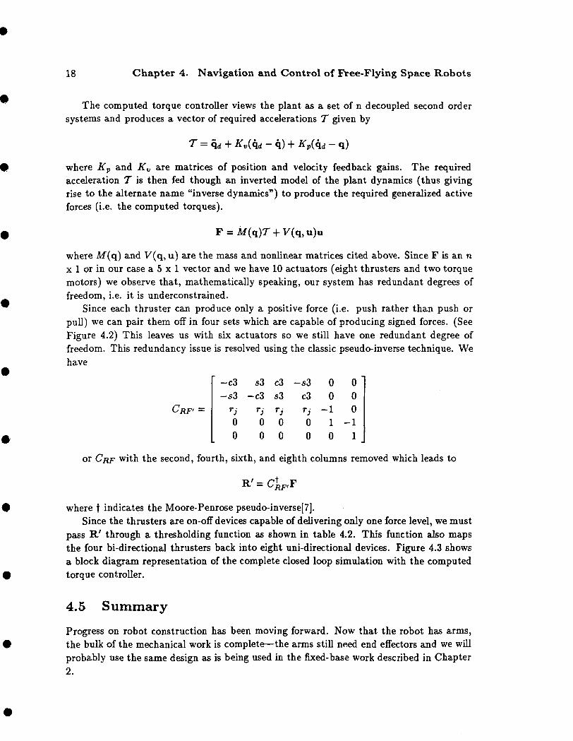
The computed torque controller views the plant as a set of n decoupled second ordersystems and produces a vector of required accelerations T given by

T = - q) - q)

where Kp and Kv are matrices of position and velocity feedback gains. The requiredacceleration T is then fed though an inverted model of the plant dynamics (thus givingrise to the alternate name "inverse dynamics") to produce the required generalized activeforces (i.e. the computed torques).

F = M(q)T + V(q,u)u

where M(q) and V(q, u) are the mass and nonlinear matrices cited above. Since F is an nx 1 or in our case a 5 x 1 vector and we have 10 actuators (eight thrusters and two torquemotors) we observe that, mathematically speaking, our system has redundant degrees offreedom, i.e. it is underconstrained.

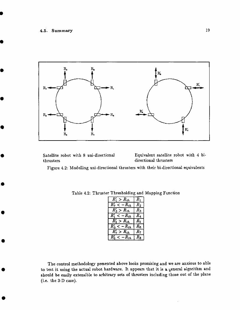
Since each thruster can produce only a positive force (i.e. push rather than push orpull) we can pair them off in four sets which are capable of producing signed forces. (SeeFigure 4.2) This leaves us with six actuators so we still have one redundant degree offreedom. This redundancy issue is resolved using the classic pseudo-inverse technique. Wehave

CRF> —

or CRF with the second, fourth, sixth, and eighth columns removed which leads to

R = ^RF'F

where f indicates the Moore-Penrose pseudo-inverse[7).Since the thrusters are on-off devices capable of delivering only one force level, we must

pass R' through a thresholding function as shown in table 4.2. This function also mapsthe four bi-directional thrusters back into eight uni-directional devices. Figure 4.3 showsa block diagram representation of the complete closed loop simulation with the computedtorque controller.

4.5 Summary

Progress on robot construction has been moving forward. Now that the robot has arms,the bulk of the mechanical work is complete—the arms still need end effectors and we willprobably use the same design as is being used in the fixed-base work described in Chapter2.

' -c3-53

Tj

00

53

-c3Tj

00

c353

00

-53

c3

00

00

-110

0 '00

-11

4.5. Summary 19

R.

•R,

•R.

Satellite robot with 8 uni-directionalthrusters

Figure 4.2: Modelling uni-directional thrusters with their bi-directional equivalents

Equivalent satellite robot with 4 bi-directional thrusters

Table 4.2: Thruster Thresholding and Mapping Function

R(R'7 < -

's > Rth

R{ < -R'

#7 > RthR' < -

Ri

Re

Rs

The control methodology presented above looks promising and we are anxious to ableto test it using the actual robot hardware. It appears that it is a general algorithm andshould be easily extensible to arbitrary sets of thrusters including those out of the plane(i.e. the 3-D case).

20 Chapter 4. Navigation and Control of Free-Flying Space Robots

4.6 Future Work

Now that the arms are nearly complete, our emphasis can shift to the robot's electricalsystems which make up the "analog layer" of our modular design. This layer which wasdescribed in detail in an earlier report will contain replaceable battery packs, DC-to-DCpower converters, and an analog card cage containing sensor and driver electronics, powerdistribution and control circuitry, and safety monitoring and cutout devices.

4.6. Future Work 21

(

<?•r

*̂

1

L

r~»»v .̂c ?o -5

"S 8. .IIIs

L-

>

«— .

s•4\^

\ \•*y

(*,

^

0$

L

ftj

t

"S,f\^y

k

(^

:

»

ia<

^

a~\

— »

?^fc^^4

\

%\ \

•3

5)

j

\

1

5"\

sJ :

2

.'/ ^

^(\ , t

^

?

9>

> cv.

».

.«

ENry

f\

TJ> c

L\ry

1ar

§

ouVs

*

-a0)

toSo

81•8 1

5 £

abO

22

Chapter 5

Locomotion Enhancement viaArm Pushoff (LEAP)

Warren J. JasperRoberto Zanutta

5.1 Introduction

To perform complex assembly tasks, an autonomous vehicle needs to move from one placeto another. The use of propellants may not be ideal because of cost and safety factors. Also,the use of thrusters may disturb the environment by impacting a target which the robot istrying to grasp. Our alternative approach is called LEAP: Locomotion Enhancement viaArm Pushoff. In LEAP, the vehicle pushes itself off from a large space object and "leaps" tothe desired resting place or simply "crawls" along an object. This is the common mode oflocomotion used by the astronauts while in the Space Shuttle. This new project was addedto investigate the problems and issues involved in autonomous space locomotion. The firstphase of the project involves: devising the experiment, deriving the equations of motionand candidate control laws, and then simulating the model to size physical parametersfor the actual experiment. The second phase encompasses design and fabrication of thevehicle, while the third phase is to experimentally verifiy the theoretical development. Thefollowing paragraphs describe the progress onphase one.

5.2 The Experiment

A new air-cushion vehicle is being designed to study LEAP. This vehicle should simulatethe motions that an autonomous space robot would perform while in the space station ormaneuvering out in space. The experiment will consist of the vehicle pushing off a barlocated on one side of the granite table, rotating 180 degs, and catching itself by graspinga bar located at the other end of the table. Ideally, one would like to complete this taskwithout the use of thrusters. However, at the point of initial release from the bar, errors

23

PRECEDING PAGE BLANK NOT FUMED

24 Chapter 5. Locomotion Enhancement via Arm Pushoff (LEAP)

Figure 5.1: The LEAP Demonstration

in the velocity of the center of mass of the vehicle can only be corrected using thrusters.To enhance the robustness of this approach, thrusters will be incorporated into the controllaws for midcourse correction. Figure 5.1 shows the robot in three configurations: pushingoff the bar, rotating, and catching itself at the other end. By incorporating crawling andleaping, the robot can position itself anywhere on the table with a minimum amount ofpropellant. This investigation complements current work done at the Stanford AerospaceRobotic Laboratory by incorporating global navigation and object manipulation into ageneral study of locomotion.

5.3 Vehicle Modelling

A great deal of design work has been done under this NASA contract in the field of multiple-arm autonomous vehicles. Because the underlying philosophy of our current robots allowsfor flexibility in design, the new vehicle will need only a few design modifications. Thesechanges include the addition of a momentum wheel subsystem and grippers. Figure 5.2shows a schematic view of the LEAP robot used for simulation. This vehicle has eightdegrees of freedom, one more than the previous design, due to the addition of a momentumwheel.

The momentum wheel is necessary to perform rotation without the use of thrusters.This reduces the propellant cost and provides linear control authority for rotation. Unfor-tunately, one can not obviate the need for thrusters completely because they are necessaryfor midcourse corrections and deceleration in free space. Also, a new gripper design isneeded which incorporates force sensing and compliance when grasping an object.

5.4. Simulation

12

25

tFigure 5.2: Schematic Drawing of the Robot

5.4 Simulation

The simulation is used as a design tool to derive specifications for the motors and thesensors as well as evaluating different control schemes. After the initial experiments, afurther iteration of the simulator will be done to increase its fidelity and to incorporatesecond-order effects. Using Kane's method, the equations of motion were derived in asimilar manner as those described in Appendix C. These equations were incorporated intothe non-linear dynamic simulation. In addition to plotting the various states of the robot,the computer, a Sun 3/160 workstation, can also produce a real-time graphics display. Thistwo dimensional display allows one to understand how the entire system is responding tovarious control laws.

To simulate the experiment, we implemented the task of leaping from one end of thegranite table to the other as a finite state machine by dividing the entire task into ten sepa-rate states. In each state, the computer uses the appropriate set of boundary conditions and

26 Chapter 5. Locomotion Enhancement via Arm Pushoff (LEAP)

control laws to achieve a desired trajectory. The control laws used are proportional deriva-tive control (PD), proportional integral derivative control (PID), and computed torque.These control laws are modified to account for discontinuities in the state due to changingboundary conditions. These conditions occur when the robot lets go of the bar and goesfrom a nonholonomic closed-loop chain configuration with four degrees of freedom to aholonomic free floating configuration with eight degrees of freedom. A similar conditionarises when the robot grasps the bar at the other end of the table, however, there is alwaysthe possibility that both arms will not grasp simultaneously, and thus we allow for twoadditional conditions.

5.5 Future Work

With the completion of the first phase, we plan to proceed to the second phase of the projectwhich includes fabrication and integration of the various subsystems into a working vehicle.This phase should last well into the Fall of 1988. Also in the second phase, we will lookinto new sensor technologyfor force and rate sensing and incorporate these sensors into thevehicle.

Appendix A

Accurate Real-time Vision Sensor

Stan Schneider

A.I The Vision Sensor Problem

Advanced end-point control of complex systems requires tracking several objects simulta-neously. End-point information to be used for control feedback must be highly accurate,and available at a high sampling rate. To provide this information, we are developing avision system capable of tracking at least four points with an error of less than one partin one thousand. Sample rates will be at least 60 times per second per target. No sys-tems currently commercially available provide sufficient performance. This report describesprogress to date in the development of this vision sensor.

A.1.1 Proposed Solution

Recent advances in CCD camera technology have made pixel-based end point detectionfeasible. At the current time, 440 by 240 pixel arrays are available with sampling ratesgreater than 60 Hz. Coupled with local processing power to provide an intelligent interface,this allows sample rates well within the above specifications. Unfortunately, the accuracy,240:1, is not acceptable for precision control. The problem thus becomes one of gleaningsub-pixel accuracy from the available data.

By utilizing the available gray scale resolution of the camera, this is practicable. In-stead of simple binary (white dot or LED) targets, we propose to use targets that varyin reflectivity, from black at the edges to near white in the center. They span an area ofapproximately 8 by 8 pixels. Thus, each pixel in the 8x8 grid contains information aboutthe location of the center. (In the noise-free case, one could calculate the distance to thecenter from each pixel exactly.) A simple, fast centroid (center-of-brightness) calculationthen yields an estimate of the actual center.

'Summary of work begun in 1986/1987 under AFOSR contract. The vision sensor system describedherein will be developed under the current NASA contract, and incorporated into the fixed-base cooperativemanipulation experiment. This appendix is included for completeness.

27

28 Appendix A. Accurate Real-time Vision Sensor

A. 1.2 Summary of Progress

A probabilistic analysis has been completed. In addition, a full simulation of the targetlocation procedure was implemented to verify the analysis. Finally, a simple experimentalsystem was constructed, and its performance measured. The results are encouraging.With the new camera that has been ordered, the above performance specification shouldbe achievable.

A.2 Theoretical Analysis

For the purposes of this discussion, we assume an JV x N pixel sub-grid. This grid issufficient to encompass the entire target area. The center of the target is calculated as thecentroid of illumination. We will calculate the centroid in one dimension only, the other isidentical.

Let:Pij represent the i, jth pixel,

S = 53 wiPij be the weighted pixel illumination, andT = ^2 p^ be the total illumination.

For our purposes, Wi is simply the distance from the center of the coordinate system,

The centroid is found simply by:

2=f (A.I)

Quantization effects are insignificant in comparison with the camera noise. Thus, thenoise can be assumed to be gaussian, and white. Now, if each pixel is corrupted byindependent gaussian noise of variance <r2, then both S and T are gaussian random variableswith:

2 = *V (A.2)

'-«o)V (A.4)«'.j

A*. = !>((«'-«o)Pv) (A.5)

We now develop an expression for the probability density function of the centroid. Thedistribution function is found by integrating over the region of s/t < z:

Fz(z}= I [°° fta(t,s)dsdt + f°° IZ fts(t,s)dsdt (A.6)J-oo.Jzt JO J-oo

Where

A.3. Simulation 29

Using the relation /^ g(x)dx = f£° g(—x)dx and Liebnitz's rule for differentiation, weobtain:

/,(*) = —Ff(z) = f°° t(fta(t, zt} + /«.(-*, -zt))dt (A.8)UZ Jo

Substitution of A.7 yields:roo _ ^oo

JO JQ

with:

A ~ —^'-rl + zWt) (A.10)

1 2 9\B = 2 (2^t(7j + 2z^3a^) (A.11)

c = sio^ + ^t2) (A.12)

K = ^T (A-13)

After integration and collection of terms, the density function is:

Here, $(x) is the error function,

°° 2-

Note that further simplifications are possible. For example, *—^ ' can be reducedtn (^»-^«)2\l\J ^^^^*)^^^^ •

°?°?In the zero mean case, C = B = 0, this reduces to the well known ratio of gaussian

densities, the Cauchy density. An interesting result is that the best estimate of the centroidis not simply the above ratio of S/T, but the much more complicated expected valueof /z(z). A rough evaluation of the actual best target center estimate can be made bysubstituting reasonable values for all the parameters (which yields //< is large, p, is nearlyzero, and a, is significantly larger than <7t). This rough analysis yields two results: 1) S/Tis a very good estimate of the maximum, and 2) the actual best estimate is always slightlysmaller magnitude (closer to zero) than S/T.

A.3 Simulation

To verify the above analysis, a full simulation of the target center calculation was imple-mented. This program allows rapid variation of such variables as: pixel signal-to-noiseratio, quantization effects, target size, target reflectivity profile, and background illumina-tion variation.

30 Appendix A. Accurate Real-time Vision Sensor

A.3.1 Simulation Description

The target is modeled as a truncated cone of variable intensity. Figure A.I depicts a typicaltarget reflectivity profile. All labeled parameters are user-selectable.

Target locations are selected randomly near the center of the grid. The camera CCDresponse is calculated by integrating the target illumination over each pixel. Gaussian noiseis added, and the value quantized to the user-specified number of levels. The target locationis then determined by the above algorithm. The program outputs raw data, average error,and an error histogram.

1.0 —

Target max.t-j>

cr

0.0 —Target radius

Target min

Background radius

Figure A.I: Simulated Target Reflectivity Profile

A.3.2 Simulation Results

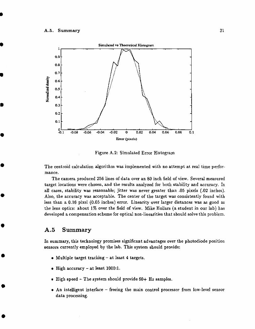
The graph in figure A.2 shows a plot of the histogram of error values obtained over 1000trials. The above probability density function is also plotted for comparison. Under realisticconditions (100:1 signal/noise amplitude; 3 pixel radius linear density targets), the methodlocated the center to better than l/10th of a pixel worst case, l/20th pixel average case.With a 440x240 pixel camera, this represents very respectable accuracy (typically 1 partin 2000!).

The centroid calculation algorithm could be improved slightly. Due to the divisionnonlinearity, the best estimate of the true centroid is not simply S/T, but a value slightlysmaller. Use of a simple scaling factor could reduce the frequency of the larger errors. Inthe case of this system, it is unlikely this effect will be significant.

A.4 Preliminary Experimental Results

Before ordering high speed equipment, a preliminary proof-of-concept experiment was con-ducted. Using an IBM PC with a commercially available low-speed frame digitizer, datafrom a standard format camera was collected. Figure A.3 shows a representative target.

A.5. Summary 31

I'•3

l

0.9

0.8

0.7

0.6

0.5

0.4

0.3

0.2

0.1

Simulated vs Theoretical Histogram

-0.1 -0.08 -0.06 -0.04 -0.02 0 0.02 0.04 0.06 0.08 0.1

Error (pixels)

Figure A.2: Simulated Error Histogram

The centroid calculation algorithm was implemented with no attempt at real time perfor-mance.

The camera produced 256 lines of data over an 80 inch field of view. Several measuredtarget locations were chosen, and the results analyzed for both stability and accuracy. Inall cases, stability was reasonable; jitter was never greater than .05 pixels (.02 inches).Also, the accuracy was acceptable. The center of the target was consistently found withless than a 0.16 pixel (0.05 inches) error. Linearity over larger distances was as good asthe lens optics: about 1% over the field of view. Mike Hollars (a student in our lab) hasdeveloped a compensation scheme for optical non-linearities that should solve this problem.

A. 5 Summary

In summary, this technology promises significant advantages over the photodiode positionsensors currently employed by the lab. This system should provide:

• Multiple target tracking - at least 4 targets.

• High accuracy - at least 1000:1.

• High speed - The system should provide 60+ Hz samples.

• An intelligent interface - freeing the main control processor from low-level sensordata processing.

32 Appendix A. Accurate Real-time Vision Sensor

Figure A.3: Example Target

• Future flexibility - Since the entire scene is available to the image processing system,further functionality could be implemented. For instance, objects in the environmentcould be identified to be used in assemblies, or mapped to be avoided. Use of simplescene analysis could also greatly benefit future cooperative tasks.

Appendix B

Serial Chain ManipulatorEquations of Motion

Ross KoningsteinThis theory for serial chain manipulators is derived using Kane's dynamical analysis

techniques. The analysis that follows assumes that the velocities v of points and angularvelocities u> of bodies in the system under consideration can be expressed in a Newtonianreference frame as follows:

«•' = 5>x«=iThis will be true if no part of the system is undergoing prescribed motions. The partial

angular velocities of bodies, and partial velocities of points, as defined by Kane[3], can beshown to be:

—v

d

This analysis will show that the elements in the matrix equation

Mil = -Nu + F

are highly structured and can be computed numerically with a very straightforward al-gorithm. In order for the algorithm to function, the partial velocities of the first chainelement, and the partial angular velocities of all chain elements need to be specified. Man-ual computation of accelerations, and force components is not required. These derivationsassume all velocities, angular velocities, momenta are expressed in a Newtonian referenceframe.

33

34 Appendix B. Serial Chain Manipulator Equations of Motion

B.I Structure in Dynamical Equations

In the Kane's Dynamical equations

Fr + F; = oThe generalized active forces are

applied appliedforces i torques j

and that the generalized inertia forces are

F;=applied appliedforces i torques j

The generalized inertia force expression, when derived for serial chains, will be examinedmore closely. Expressions for the inertial forces will be derived using the linear and angularmomenta of the bodies in the system. First, the terms due to changes in linear momentumwill be examined, then terms due to changes in angular momentum will be examined.

The linear momentum of the ith body is defined as

L' = m,V*n

where the partial linear momentum is defined by

L; = m,-vrThe inertia force caused by the acceleration of the center of mass of the ith body is:

»=l 8=1

Its contribution to the generalized inertia forces is

a=l

B.I. Structure in Dynamical Equations 35

The contribution of the changes in angular momentum will now be examined. Theangular momentum of the ith body is defined as

' = r/1* -•u?n

where the partial angular momentum is defined by

H; = r/'The inertia torque caused by the angular acceleration of the ith body is

Tt* TTt= —fi.

dt

Its contribution to the generalized inertia forces is

a=l a=l

The generalized inertia forces can be then be expressed as

All a=l a=lBodied

= - EAllBodiesi

The generalized inertia force can be separated into two components, one encompassingthe derivatives of the generalized speeds, and the other comprising all the rest.

^ - EAll 5=1Bodies!

All 5=1 5=1Bodie<i

36 Appendix B. Serial Chain Manipulator Equations of Motion

The inertia and momentum scalars which make up the mass matrix and non-linearcoupling matrix can then be evaluated as follows:

AllBodies i

AllBodies i

The generalized inertia forces can be constructed as follows:

p* _ pM i pAf1 r — x r '^r

where

s=l

The mass matrix and non-linear coupling matrix can then be used to express the equa-tions of motion of the system as:

Mu = -Nu + F

where F is the generalized active force vector which accounts for the effects of externalforces and torques applied to points and bodies in the system:

All external All extern&lforces torques

B.2 Kinetic Energy and Power Input

In a system as discussed in the previous subsections, the kinetic energy can be expressedas:

K = -bodieai

-2* »

bodiesi

rnV'-v1-

allbodieei

B.3. Formulation of Equations of Motion for Planar Serial Link ManipulatorsST

i / n \ / n \- j £ »' fev>, • £v>,*ll \r=l / \a=l /bodiesi

all \r=l / \«=1bodieai

*H r=l *=1bodies!

.bodiesi

n n

Ml . r=l»=lbodiesi

= uTMu

The power input to the system as discussed is due to work done by the actuators (armtorquers), and forces exerted on the manipulator endpoints during contact with externalobjects and can be expressed as follows:

P = F - v + T

Applied AppliedForces Torquea

= EApplied r=l AppliedForces Torques

= E| E F-v r « r +r=l \ Applied Applied

\Forces Torques

r=l

B.3 Formulation of Equations of Motion for Planar SerialLink Manipulators

A system «S, consisting of a set of serially connected rigid links in planar configuration hasa simple relationship relating link endpoint velocity to link basepoint velocity:

endpoint _ basepoint • ,-link ., basepoint to endpoint

if this is expressed using partial velocities,

vendpoint _ ^basepoint i ..link ^ _basepoint to endpoint

38 Appendix B. Serial Chain Manipulator Equations of Motion

If we define unit vector Xj to be along the link, from basepoint to endpoint, and unitvector yj to be perpendicular to Xj and in the plane of the manipulator, then we can definez, a unit vector perpendicular to the plane of the manipulator as:

Az = Xj x yi

Vector z is the same for all links i. Now, the generalized speeds l..n and the angularvelocities are related as follows:

wUnk > = mz

and the endpoint to basepoint velocity relation for link t of length /, becomes:

start to end i _ /r — <t Xj

and the partial velocity relations along the chain from start i = 1 to end n, are asfollows:

v*tarti for i = 1... r - 1*n = /,Xj for i = r

0 for i = r + 1... n

, _ J z for i = 1... r — 1U>r ~ \ 0 for i ^ T

Two additional generalized speeds, un+i,n+2 describe the motion of a designated pointone one of the chain links, for instance, the center of mass of the heaviest body, the 'robotbody'. In order to calculate the partial velocities of the mass center of each link, we definean extra coordinate set, xJ, yjf, and Zj, such that:

_start to end] /» „r — «,• x,

endpoint _ ^basepoint . /^link v -basepoint to endpoint

then, if expressed using partial velocities,

..endpoint vbasepoint i .link ,, —basepointtoendpointvr — vr -r wr A r

v;tar"' for i = 1... r - 1v*' = { /iXj for i = r

) for i = r + 1... n

B.3. Formulation of Equations of Motion for Planar Serial Link Manipulators39

The contribution of body i to the inertia scalar mT3, an element of the mass matrix M .can be determined as follows:

(m^mX'-vr + w'* -i'7'* •<•»:*for the planar system, this reduces to

m V - /

^ " I

- ^bodies i m' vr* ' VJ* for i ± r

" Ebodies i m' vJT - vJT + I'"- for n = r = s

where

and

u>Unki = u,-z

the sum of the effects of all bodies, which build a complete inertia scalar.

bodies icase r = s = j

= m'' vf • vf + m'vf1-1'* • V;>+1)* + . . .

= m

. * (r)'i ( j+1 i J+3 i ^ endj endj

"*" \ "*" ~* ') 3 J

case r 7^ s,k = max(r,s)

= mk lj*y^ •

-I- m + • • • v™k • vf dk

a similar derivation for the 'non-linear' momentum scalar terms:

where

u4* • H' = 0

In the planar configuration, no torques due to changes in orientation of the angularmomentum vector of any of the bodies occur.

If we define

40 Appendix B. Serial Chain Manipulator Equations of Motion

where

k = max(r,s)

then the inertia and momentum scalars for the mass and non-linear coupling termsmatrices can be expressed as:

m — m* vend n vend nmrs — m., v v.+mk C*1—*^ "end n

and if j = r = s

similarly, the expression for the non-linear coupling term matrix scalars is:

„ _ m* vend n -end nnrs — mT3 vr vs

if s> r+mfc (/Jyy v-d n

if r > s

B.4 Control Specification Equations

This section deals with the means whereby control specifications can be expressed in termsof quantities expressed or derived in the previous chapters. We wish to be able to determinethe Jacobian scalars jr, which form a Jacobian matrix of the form:

The endpoint velocity can be expressed in terms of its partials as:

n+2endpoint _ V^ vendpointu

r=l

and therefore endpoint velocity can be expressed in terms of speeds along the inertialV and 'y' directions, that is, along unit vectors x and y:

B.5. Nonholonomic Constraints: Closed Chain 41

n+2...x endpoint X "• endpointv — 7 ^ vr • x. UT

r=ln+2

yy endpoint _ V^ vendpoint . ^

r=l

the elements of the Jacobian are therefore:

3i. = v<ndpoint-x

J2. = v<ndpoint-y

if the endpoint is at the tip of the manipulator, then these partial velocities are exactlythe same as the ones used in the dynamical derivations.

The control specification, assumed here to be an acceleration specification for the end-point, is determined from the following expression:

the derivative of the Jacobian can be determined from quantities used in the dynamicalequation formulation:

B.5 Nonholonomic Constraints: Closed Chain

In a dynamical system with nonholonomic constraints, the generalized speeds Ui..n are notindependent, rather, one (or more) are dependent on the rest. In the system considered, aserial chain of bodies, this condition can arise when the two ends of the chain touch andare held together, either by a pin joint, or rigidly. The case of a pin constraint on the twodimensional manipulator, a nonholonomic constraint situation, will be analyzed, and theconstraint equations wiD be expressed in terms of quantities used in the derivations fordynamical analysis.

The constraint of endpoint closure is described by:

vstarti _ yendn

expanding this into partial velocities,

r=l r=l

42 Appendix B. Serial Chain Manipulator Equations of Motion

It is evident that by dot multiplication with two vectors, this vector equation can bereduced to two scalar equations, for the two-dimensional manipulator we are studying. Ifwe choose the vectors such that each is perpendicular to the partial velocity of the endbodies, then the two equations decouple and the last two generalized speeds can be solvedfor explicitly. Two candidate vectors to accomplish this are the derivatives of the partialvelocity vectors of the last two links: v*ndn and v^""1, since these vectors are guaranteedto be perpendicular to their respective partial velocities. This is proven by the fact that

vbody i _ ^body i x ybody i

If we use these two vectors to separate the vector constraint equation into two scalarconstraint equations, we get:

vstartl . vbody i^ _ yendn . vbody i^

r=l r=l

we note that

=

v*' = oso that the two constraint equations are:

n0 =

r=ln

0 =r=l

These equations are decoupled for u\ and un and can be rearranged to pick out theseterms explicitly:

n-l

r=2n-l

vn . vn _ _ V^ vn • nvr vn ~ / ; vr vn

r=2

such that the reduced set of independent speeds, ui..n, can be expressed as:

.where

B.5. Nonholonomic Constraints: Closed Chain 43

AClr =

ACnr =

if j - 1 = r CJT = 1

if j - 2 = r

• n v iT^n-1 vnZ^r=? vr for r = l..n

r = 1 } forr = n + l , n

Cjr = 0 } for all other j, r

The constrained equations of motion can then be formulated as follows:

Mui..n = -Nui..n+2 + F1--n

where

M = CMCT

N = C (N - MCT)

F A CF

44

Appendix C

Derivations of the Equations ofMotion for LEAP Vehicle

Warren Jasper. J

C.I Definitions of the Generalized Speeds

Using Kane's method for deriving the equations of motion, the following list defines thegeneralized speeds.

Ui = AvB* • bi = qi cos(g3) + qi sin(g3)

u2 = AvB' • 62 = 92 cos(g3) - ft sin(93)

u3 = Au>B • k = 93

u4 = A&C • k = 4s + 94

us = AuD • k = 93 + 94 + 95

ue = AvE • fc = 93 + 96

«? = AuF • k = 93 + 96 + 97

us = Au° • k = q3 + 9s

Using these definitions for the generalized speed, the velocities of the points of interestbecome:

AvB' = U 1 b 1 +u 2 b 2 (C.I)AvPs = «i 61 + u2 62 + «3 /i ^ (C.2)

2 - u4l3ci (C.3)

2 (C.4)

45PRECEDING PAGE BLANK NOT FILMED

46 Appendix C. Derivations of the Equations of Motion for LEAP Vehicle

AvD' = ui&i + u262 + U3/ir2 + u 4 /4C 2 + U5/5d2 - u5l6di (C.5)AVP* = Ui 6j + U2 &2 + «3 'l »*2 + ^4 /4 C2 + U5 /7 <J2 (C-6)

62 + U3 /8 T-4 (C.7)

&2 + u3l&r4 + u6lge2 - u6/10ei (C.8)

&2 + "3*81*4 + U6/11 62 (C.9)

«6 *11 C2 + U7 /12 / 2 - U7/13/J (C.10)

2 + U?Jl4/2 (C.ll)

C.I.I Accelerations

By differentiating the above velocities with respect to time in the reference frame A, thefollowing eight accelerations of interest become:

AaB' = iii &i + u2 62 — u2ua fej + ujua 62

^a0* = ui &i -(- it2 62 — u2U3 61 + ujUs 62 + ^3/1 r2 -(- ti4/2 c2 —

- U42/2Ci - U4

2/3C2

aP' — u\ 61 + u2 62 — u2us 61 + uiuz 62 + 03/1 r2 + i4/4 c2 +

iisk di - u5/6 di - u32/i ri - ti4

2/4 GI - tt52/5 dj - u5

2/6

62 + U3/8 r4 + U6/9 C2 -

= iii 61 + w2 62 — u2U3 61 + uiu3 62 + u3/8 r4 -|- ii6/n e2 +

W?'l2 /2 - "7^13 /I - U32/8 r3 - U6

2/ll C! - W72/i2 /a - U7

2/13

= ill 6l + «2 ^2 - «2"3 &1 + Ul«3 &2 + W3/15 T6 - U32li5 T5

2 + "3^1 »*2 + «4/4C2 +

4 + u6n e2

- U72/14 fl

C.I.2 Partial Velocities and Partial Angular Velocities

The next step in the derivation of the equations of motion is to calculate the partialvelocities AvPi and partial angular velocities Au)B where

V * 2£1 (c.i3)

V =A 8AuB

8UT '̂"'

The following is a table of the partial velocities and partial angular velocities for the robot.

C.I. Definitions of the Generalized Speeds 47

r12345678

A R* A P- 4 /"** A P. A 7")* 4 P•T**«*J 79 3 71 V 75 75 ^

6162000000

Oj.

v9

/ir2

00000

61&2

/ir2

/2 C2 - /3 Ci

0000

61&2

/ ir2

/4C2

0 -000

bib2

•1 **2

/4C2

5 ^2 — k di000

6162

/ 1 T*2

14 C2

/7<*2

0

0

0

A E'

12345678

&i&2

^T-4

0

0

0 I

00

Q-)

vO

/8»"4

0

0

ge 2_/ l o e i

00

Q-j

09

^8^400

/ne2

00

i>i&2

^T-4

0

0

/ne2

^12 /2 ~ ̂ 1

0

Q-t

O1}

I*r4

00

/Uc2

3/1 'l4/2

0

6lOo

^ 1 c T*^;

00000

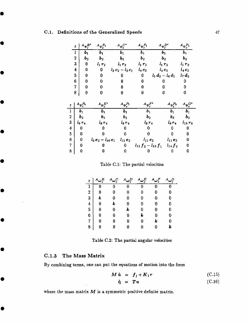
Table C.I: The partial velocities

u?:12345678

00k00000

000k0000

0000k000

00000Ik00

000000k0

0000000k

Table C.2: The partial angular velocities

C.I.3 The Mass Matrix

By combining terms, one can put the equations of motion into the form

Mu = fj + Kir

q = Tu

where the mass matrix M is a symmetric positive definite matrix.

(C.15)

(C.16)

48 Appendix C. Derivations of the Equations of Motion for LEAP Vehicle

M =

' 21 0

0 2j

22 2n

23S4 + 24£4 —

24C4 23C4

25*45 + 2e*45 —

26C45 2sC4s

27«6 + 28*6 —

2sCe 27Ce

2gS67 + 2io*67 —

210^67 2gC67

0 0

22

211

212

213*4 +

2i4C4

215*45 +

216C45

217*6 +

218C6

219*67 +

22QC67

0

23S4 +

24C4

24*4-

23C4

213*4 +

214C4

221

222*5 +

223C5

0

0

0

25*45 + 27*6 +

26C45 28C6

26545- 2856-

2sC45 27^6

2l5*45 + 2l7*6 +

2l6C45 218C6

222*5 + 0

223C5

224 0

0 225

0 226*7 +

227C7

0 0

29567+ 0

210C67

210*67- 0

29C67

219*67+ 0

220C67

0 0

0 0

226*7 + 0

227C7

228 0

0 229 .

(C.17)Where the Zi are constants and have the following definitions:

21

22

24

25

26

27

28

29

= mi + m2 +A , .

A

A

A

A

A

A

A

A

m4

i) -(m4 + m5)/i

212

= (m2 -'• ms)/i cos(^i) + (m4 + ms)/8cos(^2) +

m3)/i2 + (m4 + m5)/82 + m6/is2

?i) — ma/i'/,

^ h

sin(03)

C.I. Definitions of the Generalized Speeds 49

=

sin(0j

= -m3/i/6sin(0i) - m3/i/5cos(0i)

sin(02)

= m4?8fiosin(02) + m5f8JiiCos(02) + m4l&ls cos(02)

220 =

221 =

222 =

223 =

224 =

225 = /4 + m4(/92 + /10

2) + m5/n

226 = -

227 = ms/n/12

228 = /5

229 = ^6

The non-linear terms in u,- are found in the vector //, and with the the definitions of the2, from above, they become:

//(I) = W2U32! + U322n + U4

2(Z4S4 - 23C4) + U52(z6S45 - 25C45)

~ 27C6) + U72(Zi0S67 ~ 29C67)

U3222 - U4

2(23S4 + 24C4) - U

28C6) - U72(Z9S67 + 210C67)

24C4) - U

- Z5C45) + U2U3(Z5S45 + 26C4s)

U42(223«5 -

/7(6) = -

- 226C?)

- 29C67)

/;(8) = 0

50 Appendix C. Derivations of the Equations of Motion for LEAP Vehicle

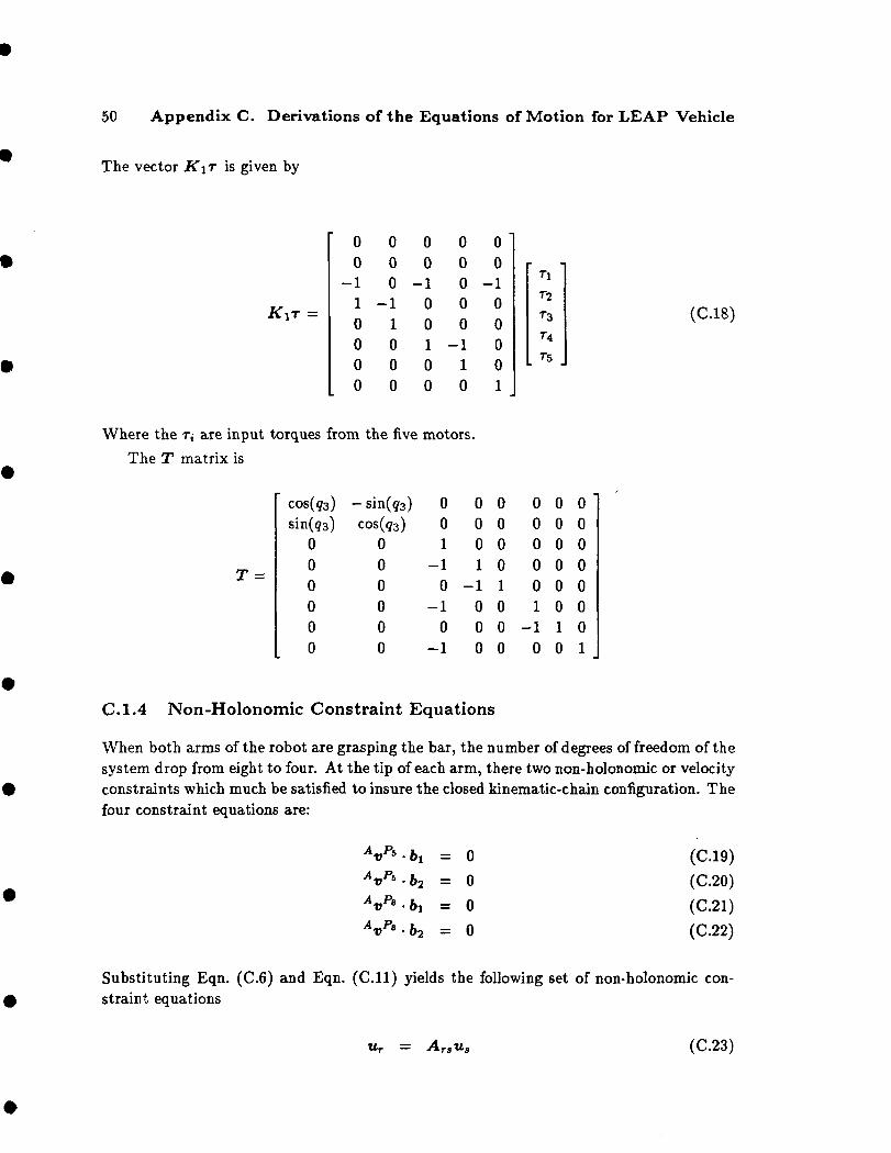
The vector K\T is given by

00

-110000

000

-11000

00

-100100

00000

-110

0 "0

-100001

- -r\T-2

7-314

. TS .

(C.18)

Where the r, are input torques from the five motors.

The T matrix is

T =

cos(g3) - sin(g3)sin(g3) cos(q3)

0 00 00 00 00 00 0

00110101

0001

-1000

00001000

000001

-10

00000010

0 "0000001

C.I.4 Non-Holonomic Constraint Equations

When both arms of the robot are grasping the bar, the number of degrees of freedom of thesystem drop from eight to four. At the tip of each arm, there two non-holonomic or velocityconstraints which much be satisfied to insure the closed kinematic-chain configuration. Thefour constraint equations are:

= 0

= 0

= 0

= 0

(C.19)

(C.20)

(C.21)

(C.22)

Substituting Eqn. (C.6) and Eqn. (C.ll) yields the following set of non-holonomic con-straint equations

ur = ATau3 (C.23)

C.I. Definitions of the Generalized Speeds 51

U4

"6

sin(?s)

sin(97)

sin((j7)

lg sisin(}7)

sin(<j7)

'11 sin(?7

Differentiating the velocities in Eqn. (C.6) and Eqn. (C.ll) with respect to time in referenceframe A and dotting the acceleration vectors with orthogonal unit vectors 61 and 62 givesthe following set of equations which expresses ur in terms of ua,u and q.

Ur = AraUs + brs (C.24)

U4

US

smfijl)

sin(94)[7 sin(g5)

/ii sm(g7)

cos(?e)

4 sin(js)

sin(g4-gilj sin(75)

ltl sm(q7)

Is sinf^e-Sj)

/4sin(?5)

/7 si

III sin(97)

With this constraint equation, one can derive the reduced set of the equations of motionby partitioning Eqn. (C.15) and adjoining the constraint equation as follows

MilM22 K lr

(C.25)

fl,

[Mn+M12^rs + (Mi2Ars)2 us =

(C.26)

52 Appendix C. Derivations of the Equations of Motion for LEAP Vehicle

C.I.5 Force Constraint

The is an alternate but equivalent formulation of the equations of motions which do notinvolve solving for the non-holonomic constraints, but rather impose a force boundarycondition at the tips to insure that the velocity at the tips of the arms is zero when thearms are grasping the bar. If Eqn. (C.15) is modified to include forces at the tip we get

M u = fj + KIT + K2fT (C.27)

is a four vector representing the normal and tangential forces exerted by thearms at points P5 and P&.

Where /j> is a lour vecior represeuuibar on the arms at points P5 and P&.

cos(q4 + 95) 94 + 95)

sin94 + 95 cosq4 +sin(94 + 9s - #1 ) f i cos(94 + 9s

-/4sin(95) -/4cos(9

000

- cos(96 + 97— sin(9e + 97'

—/gsin(96 + 97 —00

-/u sm(g7)00

sin(g6 + g7)- cos(g6 + 97)

00

-In cos(g7)-/14

0

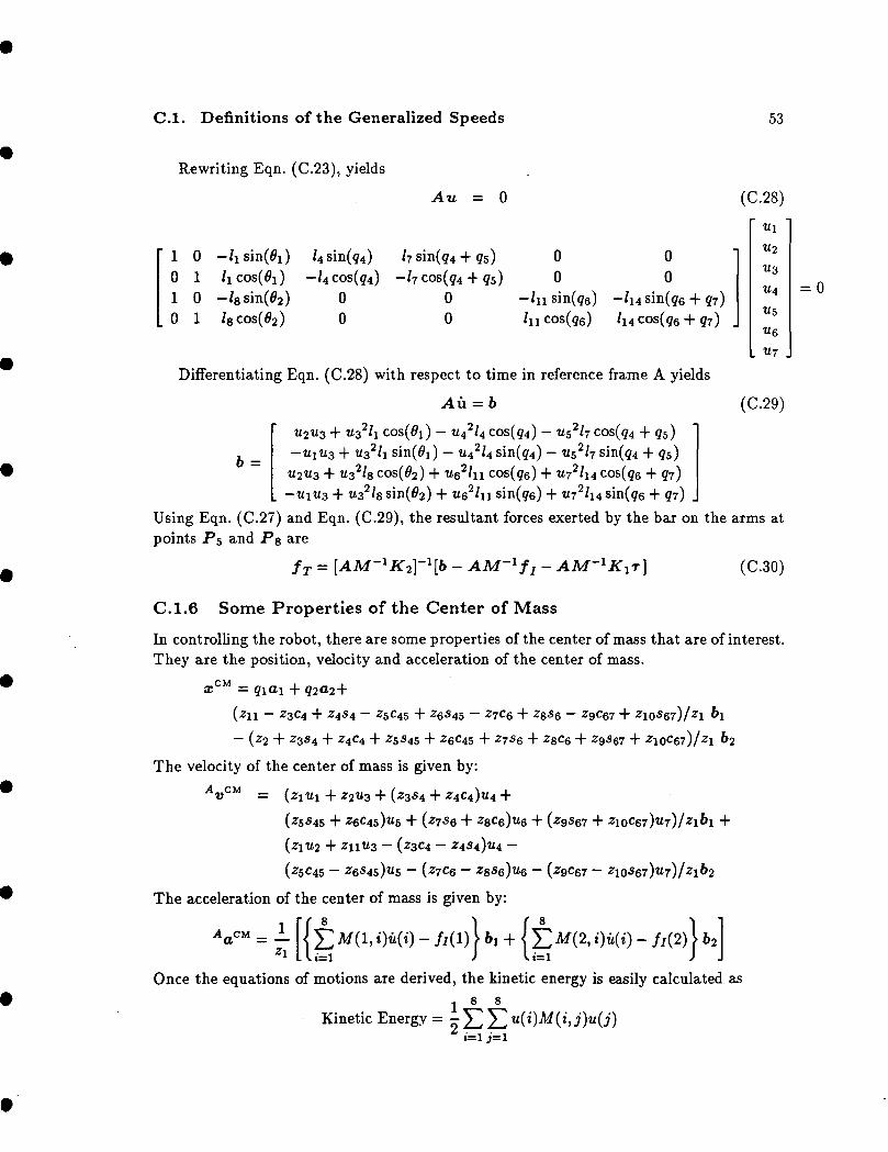
C.I. Definitions of the Generalized Speeds 53

Rewriting Eqn. (C.23), yields

1 0 -/isin(0i) /4sin(94) /?0 1 /icos(#i) -/4cos(94) -/1 0 -J8sin(02) 00 1 /8cos(6>2) 0

Au = 0 (C.28)

00

0 00 0

-In sin(g6) ~/i4 sin(g6 + 97)In cos(g6) /14 cos(g6 + g7)

Differentiating Eqn. (C.28) with respect to time in reference frame A yields

Au = b

= 0

U6

b =

Au = b

i cos(#i) - u42/4 cos(g4)

2/i sin(^i) - u42/4sin(?4)n cos(g6)

(C.29)

cos(q4

7sin(g4 + 9s)4 cos(g6 + 97)

Using Eqn. (C.27) and Eqn. (C.29), the resultant forces exerted by the bar on the arms atpoints P5 and Pg are

fT = [AM-lK2]~l[b - AM"1// - AM-^Kir] (C.30)

C.I. 6 Some Properties of the Center of Mass

In controlling the robot, there are some properties of the center of mass that are of interest.They are the position, velocity and acceleration of the center of mass.

- Z5C45

Z4C4 + Z5S45 + Z6C45

The velocity of the center of mass is given by:

Z4c4)u4

Z8C6

AvCM =

- Z4s4)u4 -

- Z6s45)u5 - (z7c6 - zss6)ue - (zgce7 -

The acceleration of the center of mass is given by:

Aa™ = 1 [(f>(l, •>(••) - //(I)} 61 + (i>(2,iXO - //(2)1 62!Zl LU=i ) Lt=i ) JOnce the equations of motions are derived, the kinetic energy is easily calculated as

, 8 8

Kinetic Energy = - ̂ ^ u(i)M(i, j}u(j)* t=i j=i

54