Control Engineering Practice 53 (2016) 124–138

Contents lists available at ScienceDirect

Control Engineering Practice

http://d0967-06

n CorrE-m

eva.zacecelikovs

journal homepage: www.elsevier.com/locate/conengprac

Bridging the gap between the linear and nonlinear predictive control:Adaptations for efficient building climate control

Matej Pčolka a,n, Eva Žáčeková a,n, Rush Robinett b, Sergej Čelikovský c, Michael Šebek a

a Department of Control Engineering, Faculty of Electrical Engineering, Czech Technical University in Prague, Technická 2, 166 27 Praha 6, Czech Republicb Mechanical Engineering-Engineering Mechanics, Michigan Technological University, United Statesc Institute of Information Theory and Automation, Czech Academy of Sciences, Czech Republic

a r t i c l e i n f o

Article history:Received 7 June 2015Received in revised form23 January 2016Accepted 24 January 2016Available online 5 February 2016

Keywords:Model predictive controlIdentification for controlBuilding climate control

x.doi.org/10.1016/j.conengprac.2016.01.00761/& 2016 Elsevier Ltd. All rights reserved.

esponding authors.ail addresses: matej.pcolka@fel.cvut.cz (M. Pčkova@fel.cvut.cz (E. Žáčeková), rdrobine@mtu@utia.cas.cz (S. Čelikovský), sebekm1@fel.cvu

a b s t r a c t

The linear model predictive control which is frequently used for building climate control benefits fromthe fact that the resulting optimization task is convex (thus easily and quickly solvable). On the otherhand, the nonlinear model predictive control enables the use of a more detailed nonlinear model and ittakes advantage of the fact that it addresses the optimization task more directly, however, it requires amore computationally complex algorithm for solving the non-convex optimization problem. In this pa-per, the gap between the linear and the nonlinear one is bridged by introducing a predictive controllerwith linear time-dependent model. Making use of linear time-dependent model of the building, thenewly proposed controller obtains predictions which are closer to reality than those of linear time in-variant model, however, the computational complexity is still kept low since the optimization task re-mains convex. The concept of linear time-dependent predictive controller is verified on a set of nu-merical experiments performed using a high fidelity model created in a building simulation environmentand compared to the previously mentioned alternatives. Furthermore, the model for the nonlinearvariant is identified using an adaptation of the existing model predictive control relevant identificationmethod and the optimization algorithm for the nonlinear predictive controller is adapted such that it canhandle also restrictions on discrete-valued nature of the manipulated variables. The presented com-parisons show that the current adaptations lead to more efficient building climate control.

& 2016 Elsevier Ltd. All rights reserved.

1. Introduction

Presently, energy savings and reduction of energy consumptionin buildings are some of the most challenging issues facing theengineering community. The reason is straightforward and thenumbers speak for themselves – up to 40% of the total energyconsumption can be owed to the building sector (Perez-Lombard,Ortiz, & Pout, 2008). More than half of this 40% is consumed byvarious building heating/cooling systems. Therefore, the recentsignificant emphasis on the energy savings in this area is right ontarget and can be observed in recent years. For example, thestrategy of the European Union called “20–20–20” (EuropeanEconomic & Social Committee, 2005) should be mentioned. In-tended to be followed by all of Europe through the year 2020, thisstrategy aims at 20% reduction of the use of primary energysources and production of the greenhouse gas emissions, and the

olka),.edu (R. Robinett),t.cz (M. Šebek).

renewable energy sources are expected to provide 20% of theconsumed energy. With the clearly evident need for savings in thearea of the building climate control, improvements can be foundwhen considering the latest control techniques.

Model Predictive Control (MPC) is one of the most promisingcandidates for an energetically efficient control strategy (Pčolka,Žáčeková, Robinett, Čelikovský, & Šebek, 2014a, 2014b). This wasalso demonstrated within the framework of the Opticontrol pro-ject. One research team at ETH Zurich (Switzerland) showed vianumerous simulations that using MPC instead of the classicalcontrol strategies achieves more than 16% savings (Gyalistras &Gwerder, 2010; Oldewurtel et al., 2010) depending on the buildingtype. If one considers real operational conditions, these savingscan be even higher when the MPC is modified appropriately forthe conditions. This was shown by teams from Prague (Prívara,Široký, Ferkl, & Cigler, 2011; Žáčeková & Prívara, 2012 and UCBerkeley (Ma, Kelman, Daly, & Borrelli, 2012) where the actual costsavings were even better than the theoretical expectations (27%and 25% reduction of the energy consumption, respectively).

However, MPC suffers from several drawbacks including thecomplexity of the optimization routine and the need for a reliablemathematical model of the building. In order to be feasible and

M. Pčolka et al. / Control Engineering Practice 53 (2016) 124–138 125

computable, simplified formulations are often considered. More-over, linear models are usually assumed and exploited by theoptimizer. Therefore, in the majority of the MPC applications, theoverall task is formulated as a linear/convex optimization problemeasily solvable by the commonly available solvers for quadratic orsemidefinite programming (Verhelst, Degrauwe, Logist, Van Impe,& Helsen, 2012; Prívara et al., 2011). Although being computa-tionally favorable and able to find the global minimum in case ofthe convex formulation of the optimization task, their dis-advantage is that they do not enable minimization of the non-linear/nonconvex cost criteria and therefore, only certain approx-imation of the real cost paid for the control is optimized. More-over, they resort to the optimization of either the setpoints or theenergy delivered to the heating/cooling systemwhile leaving all itsdistribution to the suboptimal low-level controllers which canlead to a significant loss of the optimality gained by the MPC.

In several recent works, the effort to take the nonlinearities(caused either by the dynamical behavior of the building or by thecontrol requirements formulation) into account within the opti-mization task can be found (Ma et al., 2012, 2011). In this paper,we discuss both possibilities for the zone temperature control (thelinear and the nonlinear MPC) and moreover, we bridge the twobanks of the gap between the nonlinear and the linear variant ofthe MPC by introducing linear model that changes in time. Suchmodel can describe the building dynamics in a more reliable andflexible way than the original linear model while it still keeps thelow complexity of the optimization task (since with the linearmodel, the optimization task to be solved remains convex). Theway of obtaining a time-varying model is described and the resultsof the linear predictive controller with linear model that changesin time are compared with the results of the original (linear andnonlinear) MPCs.

It should be mentioned that a good predictive controller relieson a good system dynamics predictor and therefore, we focus onthe identification of such reliable multi-step predictors as well.The MPC employs optimization over certain given predictionhorizon and this fact should be taken into consideration also in thedesign of the identification procedure. Unlike the commonly usedidentification methods (PEM, Ljung, 1999) which provide modelsthat are able to predict well only over short horizons, the methodsbased on minimization of multi-step prediction errors (MRI –

model predictive control relevant identification, Laurí, Salcedo,Garcia-Nieto, & Martínez, 2010) offer models with more attractiveprediction properties. Therefore, we exploit the MRI for identifi-cation of both linear and nonlinear models. While several pub-lished works deal with application of MRI for estimation of para-meters of linear models (Chi, Fei, Zhao, Zhao, & Liang, 2014; Shook,Mohtadi, & Shah, 1991; Zhao, Zhu, & Patwardhan, 2014), no ex-tension, to the best knowledge of the authors of this paper, hasbeen provided for estimation of parameters of nonlinear models.Moreover, even the linear version of MRI in the literature is usuallyvalidated only on simple artificial examples. On the other hand,this paper presents application of both the linear and the newlyproposed nonlinear MRI versions on much more complex andrealistic example of building model identification.

Furthermore, a very important practical aspect of the buildingtemperature control is addressed in this work as well. In real-lifebuilding applications, water pumps are a crucial part of the ac-tuators used to manipulate the optimized input variables. Thesewater pumps possess nonlinear output dynamics where theamount of mass flow rate which can be provided by the pump isoften quantized. Therefore, the achievable water mass flow ratesbelong to a countable set of discrete values rather than to a con-tinuous interval. The appropriately designed control algorithmshould take this information properly into account. This can beperformed in several ways: (1) mixed-integer programming

techniques can be employed, (2) additional postprocessing afterthe calculation of the optimal inputs can be applied, or (3) the(originally continuous-valued) optimization procedure itself canbe adapted such that discrete-valued input profiles are obtained.

First of all, the mixed-integer programming approach is themost suitable one in case that one of the manipulated variablesshould belong to countable set of discrete values. However, themixed-integer programming problems are known to be NP-hard(Bussieck & Vigerske, 2010; Lenstra, 1983; Pancanti, Leonardi,Pallottino, & Bicchi, 2002) and their solution using mixed-integerprogramming solvers requires massive computational power.Furthermore, the majority of reliable currently available mixed-integer solvers able to handle nonlinear system description/non-linear optimization criterion are not free for industrial use. Sincethe computational burden caused by solving the mixed-integerprogramming task is huge and it is in direct opposite to the ex-tensive effort to simplify the control schemes and systems used inbuildings, this direction is not suitable. Instead of formulating thebuilding temperature control problem as a mixed-integer pro-gramming task, the other two mentioned options (additionalpostprocessing and adaptation of the continuous-valued optimi-zation procedure) are elaborated in the current paper.

The paper is organized as follows: Section 2 illustrates theproblem of the building climate control on a simple example. Boththe building and the heat delivery system description are pro-vided. Furthermore, control performance criterion, comfort re-quirements and restrictions are introduced. In Section 3, themodels supplying predictions to the model-based controllers aredescribed. The nonlinear model is derived in Section 3.1 based onthe thermodynamics while for the linear model, the assumedsimplifications are presented in Section 3.2. The linear time-varying model is presented in Section 3.3. A new approach to es-timating parameters of the nonlinear model with respect to themulti-step prediction error minimization criterion proposed inSection 3.4. Two alternative versions of this approach are pre-sented which are some of the main contributions of this paper. Allmodels are verified on the data set obtained from TRNSYS en-vironment and their results are discussed. Section 4 describes thecontrollers including the low level re-calculation (for the linearMPC) and the nonlinear optimization routine (for the nonlinearMPC). In order to address the discrete-valued nature of part of theconsidered actuators, the nonlinear MPC optimization routine ischanged in two ways: either a naive additional post-processing isemployed or the mid-processing iteration (which is another maincontribution of this paper) is incorporated into the routine. InSection 5, building behaviors of all proposed controllers are in-vestigated and their results are presented and examined. Section 6draws conclusion of the paper.

2. Problem formulation

In this section, the description of the building, constraints andthe evaluative performance criterion are formulated.

2.1. Building of interest

The building under our investigation is a simple mediumweight one-zone building modeled in the TRNSYS16 (University ofWisconsin-Madison, 1979) environment, which is a high fidelitysimulation software package widely accepted by the civil en-gineering community as a reliable tool for simulating the buildingbehavior.

The building considered in this paper is a medium sized onewith a size of 5�5�3 m and a single-glazed window (3.75 m2)placed in the south-oriented wall. The Heating, Ventilation and Air

Fig. 1. A scheme of the modeled building.

Fig. 2. A scheme of heat distribution system.

Table 1List of the specific parameters.

TZmin (°C) 22/20 PW (–) 2.6199

HT (€/kWh) 0.1168 α0 (–) 9LT (€/kWh) 0.0502 α1 (–) × −9.25 10 3

TSt (°C) 60 α2 (–) × −1.875 10 6

[ ]m m, [15,60] ΔT (°C) 5

M. Pčolka et al. / Control Engineering Practice 53 (2016) 124–138126

Conditioning (HVAC) system used in the building is of the so-called active layer type. Technically, the HVAC system consists ofTABS (thermally activated building system) – a set of metal pipesencapsulated into the ceiling distributing the supply water whichthen enables thermal exchange with the concrete core of themodeled building consequently heating the air in the room. Thisconfiguration corresponds to the commonly used building heatingsystem in the Czech Republic. Ambient environmental conditions(ambient temperature, ambient air relative humidity, solar radia-tion intensity and others) are simulated using TRNSYS Type15 withthe yearly weather profile corresponding to Prague, CzechRepublic.

Fig. 1 shows a sketch of the building HVAC system configura-tion, the “building” variables and the environment variables. Re-garding the building inner variables, four of them are consideredto be available – zone temperature TZ, ceiling temperature TC,temperature of the return water TR and temperature of the south-oriented wall TS. From the environmental influences, solar radia-tion Q S and outside-air temperature TO are taken into account asdisturbances while the supply water temperature TSW and themass flow rate of the supply water m are the controlled inputvariables. The TRNSYS model in this configuration offers a goodnumerical test-bed to compare the control approaches, and theresults obtained with this model can be generalized without anyloss of objectivity.

The next step is to describe the heat distribution system. In theapplication presented in this paper, the configuration of theheating system as shown in Fig. 2 is considered. Clearly, the sto-rage tank plays a key role as the sole heat supplier in this system.In fact, having obtained the requirements for the supply watertemperature TSW and the supply water mass flow rate m, these twovalues are “mixed” using the return water with the temperature TRflowing into the building inlet pipe through the side-pipe at themass flow rate ms and the water from the storage tank which iskept at certain constant value TSt (in this paper, = °T 60 CSt isconsidered) and can be withdrawn from the tank at mass flow ratemSt . Based on this, the following set of equations can be written forthe upper three-way valve:

= +

= + ( )mT m T m T

m m m . 1SW St St S R

St S

which can be further rewritten into an expression for the

calculation of the storage water mass flow rate,

= ( − )( − ) ( )

m mT TT T

.2St

SW R

St R

Having the return water temperature values at disposal andextracting the storage water with the temperature of TSt at themass flow rate mSt , both the supply water temperature and supplywater mass flow rate related to the heating requirements can beachieved.

2.2. Control performance requirements

Considering the building climate control, one of the most im-portant tasks is to ensure the required thermal comfort which isspecified by a pre-defined admissible range of temperatures re-lated to the way of use of the building (office building, factory,residential building, etc.). Under the weather conditions of middleEurope with quite low average temperatures where heating isrequired for more than half of year, the thermal comfort satisfac-tion requirement can be further simplified such that the zonetemperature is bounded only from below. Since an office buildingwith regular time schedule is considered, the lowest admissiblezone temperature ( )T tZ

min whose violation will be penalized isdefined as a function of working hours as

( ) = °° ( )

⎧⎨⎩T t22 C from 8 a. m. to 6 p. m .,

20 C otherwise. 3Zmin

Then, the thermal comfort violation is expressed as

( ) = ( ( ) − ( )) ( )CV t T t T tmax 0, . 4Zmin

Z

Besides the comfort violation CV(t), the price paid for the op-eration of the building is penalized in the cost criterion as well.Coming out of the considered structure of the building and itsenergy supply system, the monetary cost includes the price for theconsumed hot water and the electricity needed to operate the twowater pumps. While the hot water price PW is considered constant(see Table 1), the electricity price PE(t) which applies to the op-eration of the supply and storage water pumps is piece-wiseconstant and similar to the lowest admissible zone temperature

M. Pčolka et al. / Control Engineering Practice 53 (2016) 124–138 127

profile, it depends on the working hours as follows:

( ) =( )

⎧⎨⎩P tHT

LT

from 8 a. m. to 6 p. m .,

otherwise. 5E

In order to bring the presented case study closer to reality, thevalues of high and low tariff (HT and LT) have been chosen in ac-cordance with the real prices approved by the Regulatory Officefor Network Industries of Slovak Republic (R.O. for Network In-dustries, 2011). The exact values of HT and LT in €/kWh are listed inTable 1.

Thus, the overall performance criterion over a time interval⟨ ⟩t t,1 2 is formulated as

∫ ∫ ( )ω= ( ) + ( )( ( ) + ( )) + ( )

J CV t t P t P m P m P m td d .6t

t

t

t

E C C St W St1

2

1

2

Here, ω is the virtual price for the comfort violation CV(t) which isdefined by Eq. (4) and P mW St represents the cost paid for theconsumed hot water. Time-varying electricity price is expressed asa function of time by Eq. (5) and the power consumptions of thewater pumps corresponding to m and mSt can be calculated as aquadratic function of the particular mass flow rate,

α α α

α α α

( ) = + +

( ) = + + ( )

P m m m

P m m m

,

. 7

C

C St St St

0 1 22

0 1 22

The parameters α0,1,2 are listed in Table 1.Let us note that since the criterion (6) specifies the control

requirements for the control of a building in a very compact form,all considered controllers will be evaluated and compared ac-cording to this criterion.

2.3. Constraints

In order to ensure proper functionality of the heat distributionsystem depicted in Fig. 2, the following technical constraints im-posed on the manipulated variables need to be taken into account.

First of all, the constraints on mass flow rates which can beachieved by both the supply water pump and storage water tankpump need to be respected. The upper bound of the mass flowrates is given by the maximal power of the considered pumps.Technically, the lower bound on the supply water mass flow rate mand storage tank mass flow rate mSt is zero, however, the supplywater pump is required to always maintain some nonzero supplywater mass flow rate. To prevent the supply water pump fromdamage resulting from water overpressure potentially caused bythe storage tank pump, the storage tank mass flow rate must neverexceed the supply water mass flow rate. Due to this, the mass flowrate of the supply water and the storage tank mass flow rate arebound together by the relation ≤ m mSt . The last mass flow rateconstraint results from a common feature of the water pumps thatare very often multi-valued and cannot set the mass flow rate witharbitrarily small sensitivity. Therefore, the mass flow rate valuesmust belong to a countable admissible set of discrete values.

The second group of constraints is imposed on the supplywater temperature. Since the storage tank is the only source of hotwater and no additional heater that could increase the watertemperature to values higher than TSt is considered, it is obviousthat the highest required supply water temperature must be lowerthan or equal to storage water temperature. However, the heatlosses caused by the transportation of the storage water should bealso reflected and therefore, it is more realistic to consider theupper constraint for the supply water temperature to be severaldegrees lower than the storage water temperature. Last of all, letus note that a situation which requires a value of TSW to be lowerthan the return water temperature TR would mean negative sto-rage water mass flow rate mSt , which can not be practically

realized. On the other hand, it is also obvious that such TSW re-quirement really cannot be satisfied as only the hot water storageis considered in this configuration. With no cold water storageneither water chiller provided, the temperature of the supplywater cannot be decreased below the return water temperatureand the active cooling mode is not allowed.

Since the storage water mass flow rate is not an independentvariable and is uniquely given by the supply water mass flow ratem and supply water temperature TSW, the constraints for storagewater mass flow rate can be omitted. To sum up, the abovementioned technical constraints are mathematically formulated asfollows:

≤ ≤ ∈ = { | = × ∈ }

{ } ≤ ≤ − Δ ( )

m m m

m M m m a q a

T T T T T

, ,

max , . 8st

R SW SW St

adm a a

Parameters m, m and ΔT are provided in Table 1. Several dif-ferent values of quantization steps qst were considered in thiswork and their exact values are specified later.

3. Modeling and identification

In this section, the derivation of models for the particular var-iants of the MPC (being one of the crucial part of the whole controlapproach) is described and explained. A special emphasis is put onexplanation and description of Model Predictive Control RelevantIdentification (MRI) approach, the identification procedure pro-viding mathematical models with good prediction behavior onwider range of prediction horizons.

3.1. Nonlinear model (NM)

In the current paper, the methodology that is widely used formodeling of heat transfer effects in buildings (ASHRAE, 2009;Barták, 2010; Lienhard, 2013) is followed. As explained in thededicated literature, several physical phenomena need to be con-sidered to obtain an appropriate structure reliably describing thebuilding behavior. The most crucial aspects influencing the ther-modynamics within the inspected zone are:

1. Convection from walls: This phenomenon occurs when fluid (inthis case the zone air) moves along the body (wall) with dif-ferent surface temperature. It affects both the heated wall TCand the unheated wall TS and the zone temperature TZ. Derivedfrom the well known Newton's cooling law, the heat flux qW ,convcaused by convection can be expressed as

= ( − )q h T T .W W W Z,conv ,conv

In this expression, hW ,conv denotes the convection heat transfercoefficient and TW refers to temperature of one of the con-sidered walls, i.e. TC or TS.In case that the fluid is externally forced to move, the convec-tion heat transfer coefficient hW ,conv is independent of thetemperature difference −T TW Z . However, in case that the fluidmotion is caused solely by buoyant forces arisen from differenttemperatures of the fluid and the body (and thus temperature-dependent density of the fluid) and the gravitational effects, theconvection heat transfer coefficient hW ,conv is expressed as afunction of this temperature difference (ASHRAE, 2009; Lien-hard, 2013). A common and empirically proven choice is toexpress the convection heat transfer coefficient hW ,conv as aweak function of the temperature difference Δ = −T T TW Z ,typically ∝ |Δ |h TW ,conv

1/4 or ∝ |Δ |h TW ,conv1/3 (Lienhard, 2013;

Zmrhal & Drkal, 2006). Based on the technical specification of

M. Pčolka et al. / Control Engineering Practice 53 (2016) 124–138128

the building examined in this paper (absence of the ventilationfan), the forced convection is neglected and the convection heattransfer coefficient is in accordance with ASHRAE (2009), Barták(2010), and Lienhard (2013) modeled as

= −h h T T ,W W W Z,conv ,conv

13

where hW ,conv accounts also for influence of the surface area ofthe convecting wall AW,conv. Then, the convection heat fluxqW ,conv from particular wall can be summarized as

= − ( − )( )

q h T T T T .9W W W Z W Z,conv

13

2. Mutual interactions of the walls: Out of the three possible heattransfer phenomena – conduction, radiation and convection –,the first two might apply when inspecting the mutual interac-tions between the considered walls (ASHRAE, 2009; Lienhard,2013). Conduction heat flux qcond occurs due to the presence ofcommon edges and vertices of the walls and being the simplerone, it is expressed by a formula resembling Newton's coolinglaw (Balmer, 2010; Lienhard, 2013),

= ( − )q h T T .W S C,cond cond

Here, the conduction heat transfer coefficient hW ,cond is propor-tional to the surface area of the walls and inversely proportionalto the distance between the points at which the temperaturesTC and TS are provided.Regarding the radiation, the well known Stefan–Boltzmann lawapplies:

= ( − )q h T T ,S Crad rad4 4

with hrad embracing (besides the effect of the Stefan–Boltzmannconstant) various influences such as view factor between thetwo irradiating objects, emissivity/absorptivity and the surfacearea (Balmer, 2010). In case that the temperature differencebetween the two objects is relatively small (which holds truealso for the heated and unheated wall temperatures), radiationheat flux qrad can be with sufficient accuracy approximated by alinear function of the temperature difference,

≈ = ( − )q q h T TS Crad rad rad

and the joint conduction/radiation heat flux can be thenexpressed as

= + = ( − ) ( )q q q h T T . 10W S Ccd,rd ,cond rad cd,rd

3. Effects of ambient environment: Here, influences of solar radia-tion and ambient temperature are considered. The values of thefirst of them (solar radiation) are provided in terms of the cor-responding heat flux and therefore, no further derivations arenecessary, = q Q Ssol . The latter one is assumed to be “measured”on the outer surface of the unheated wall and is assumed tovary only negligibly across the wall surface. Then, the heat fluxresulting from the different inner and outer surface tempera-tures of the wall is described in terms of conduction through thewall as

= ( − ) ( )q h T T . 11O O O S,cond

Since the heated wall contains metal piping filled with hotsupply water, the effect of the ambient temperature TO on thetemperature TC of its inner surface is neglected.Due to the presence of the window and possible associated gapsand interstices, the ambient temperature is assumed to directlyinfluence the zone temperature according to the following ex-pression:

= ( − ) ( )q h T T , 12O Z O Z O Z, ,

where the heat transfer coefficient hO Z, reflects all the abovementioned window-related leakage effects.

4. Thermal energy supplied by the manipulated variables: In thecurrently presented case, this energy is provided by the hotsupply water of the temperature TSW circulating at mass flowrate m in the metal piping encapsulated in the concrete core ofthe building. The thermal energy that is transferred from thesupply water into the concrete core can be quantified as fol-lows:

= ( − ) ( )q c m T T . 13w SW Rin

Furthermore, based on the low thermal resistivity of the metals,it is assumed that the metal piping in which the water circulateshas temperature TP only negligibly different from the returnwater, ≈T TP R. Therefore, the return water temperature can beused for expression of the conductive heat transfer from theconcrete core to the heated wall surface,

= ( − ) ( )q h T T , 14R R R C,cond ,cond

with the heat transfer coefficient hR,cond covering the effects ofthe different piping and wall materials and the distance fromthe water piping to the heated wall surface.

Based on this, thermodynamics of each of the considered innervariables of the building can be summarized:

� dynamics of the zone temperature TZ is positively influenced bythe convection from both considered walls and the heat fluxcoming from the ambient environment. Furthermore, the zonetemperature is also increased due to the presence of solar ra-diation entering the room directly through the window,

∝ ∝ ∝ ∝ ( )Tt

qTt

qTt

qTt

qdd

,dd

,dd

,dd

. 15Z

CZ

SZ

O ZZ

,conv ,conv , sol

� heated wall surface temperature TC is decreased by the amountof heat that is transferred into the zone air via convection whileit is increased by the heat resulting from mutual interactionwith the unheated wall and also by the heat transferred fromheated supply water piping,

∝ − ∝ ∝ ( )Tt

qTt

qTt

qdd

,dd

,dd

. 16C

CC C

R,conv cd,rd ,cond

� similar to the heated wall, the unheated wall is cooled down bythe convection into the zone air. Moreover, the unheated wallsurface temperature TS decreases due to the thermal exchangewith the heated wall while it is increased due to the effects ofthe ambient environment (ambient temperature TO and solarradiation qsol),

∝ − ∝ − ∝ ∝ ( )Tt

qTt

qTt

qTt

qdd

,dd

,dd

,dd

. 17S

SS S

OS

,conv cd,rd sol

� finally, the return water temperature TR is affected by the sup-plied thermal energy and further heat transfer with the surfaceof the heated wall,

∝ − ∝ ( )Tt

qTt

qdd

,dd 18

RR

R,cond in

For further use in a mathematical model, all the building innervariables are considered as the state variables of the mathematicalmodel of the building thermodynamics, = [ ]x T T T T, , ,Z C S R .Moreover, inputs = [ ]u T m,SW stand for the manipulated variablesbeing supply water temperature and the mass flow rate of thesupply water and = [ ]d T q,O sol correspond to the predictable

M. Pčolka et al. / Control Engineering Practice 53 (2016) 124–138 129

disturbances, namely the temperature of the ambient environ-ment and the solar radiation. Then, the above mentioned phe-nomena described by Eqs. (15)–(18) are captured by the followingset of differential equations:

= − ( − ) + − ( − ) + ( − ) +

= − − ( − ) + ( − ) + ( − )

= − − ( − ) − ( − ) + ( − ) +

= − ( − ) + ( − ) ( )

x p x x x x p x x x x p d x p d

x p x x x x p x x p x x

x p x x x x p x x p d x p d

x p x x p u u x . 19

1 1 2 1

13

2 1 2 3 1

13

3 1 3 1 1 4 2

2 5 2 1

13

2 1 6 3 2 7 4 2

3 8 3 1

13

3 1 9 3 2 10 1 3 11 2

4 12 4 2 13 2 1 4

To ensure admissible computational complexity of the pre-dictive controller exploiting the nonlinear model, the structure(19) was discretized using Euler discretization method consideringfixed a priori known sampling time ts (Stetter, 1973). In this paper,ts¼15 min is considered. The discretization procedure results in aseries of difference equations expressing the one-step predictionsof the system behavior,

( )

= + − ( − ) + − ( − )

+ ( − ) +

= − − ( − ) + ( − ) + ( − )

= − − ( − ) − ( − )

+ ( − ) +

= − ( − ) + ( − )

+

+

+

+ 20

x x p x x x x p x x x x

p d x p d

x x p x x x x p x x p x x

x x p x x x x p x x

p d x p d

x x p x x p u u x ,

k k k k k k k k k k

k k k

k k k k k k k k k k

k k k k k k k k

k k k

k k k k k k k

1, 1 1, 1 2, 1,

13

2, 1, 2 3, 1,

13

3, 1,

3 1, 1, 4 2,

2, 1 2, 5 2, 1,

13

2, 1, 6 3, 2, 7 4, 2,

3, 1 3, 8 3, 1,

13

3, 1, 9 3, 2,

10 1, 3, 11 2,

4, 1 4, 12 4, 2, 13 2, 1, 4,

which are more suitable for implementation of the predictivecontroller than the continuous-time model (19). To obtain esti-mates of the parameters p of the discretized structure (20), MRIapproach (whose explanation is provided later in this Section)belonging to advanced identification techniques was employed.1

3.2. Linear model (LM)

In order to simplify the model (19), let us adopt the assumptionthat the cubic roots of the temperature differences related to theheat convection are constant over the whole range of the oper-ating points of the building. This simplifies the nonlinear terms asfollows:

( )| − | − ≈ ( − ) ( )p x x x x a x x . 21i j i j i j

13

Furthermore, = ( − )q c m T Tw SW Rin is assumed to be the controlinput instead of the pair m and TSW. Based on these assumptions,the linear version of the model Eq. (20) can be summarized as adiscrete-time state space model as follows:

= + + ( )+x Ax Bu B d 22k k k d k1

with the state matrices having the following structure:

= = =

( )

⎡

⎣

⎢⎢⎢⎢

⎤

⎦

⎥⎥⎥⎥

⎡

⎣

⎢⎢⎢⎢

⎤

⎦

⎥⎥⎥⎥

⎡

⎣

⎢⎢⎢⎢

⎤

⎦

⎥⎥⎥⎥

A

a a aa a a aa a a

a a

B

b

B

b b

b b

0

00 0

,

000

, 0 0

0 0

.

23

d

d d

d d

1 2 3

5 6 8 7

9 10 11

12 13

1 2

3 4

In this model, state and disturbance variables correspond to the

1 Let us note that the parameters pi of the discrete time model (20),∈ { … }i 1, 2, , 13 , differ from the parameters pi of the continuous time model (19)

since they incorporate also the effect of the chosen sampling period ts.

previously mentioned ones and =u qin refers to the optimizedinput. The sampling period of the system has been chosen as

=t 15 mins . The model parameters a, b, bd have been estimated bya multistep prediction error minimization procedure (MRI). Forfurther details on this method, the readers are referred to Žáče-ková & Prívara (2012).

3.3. Switched linearly approximated model (SLM)

The main idea of this approach is that for a combination ofinputs u, disturbances d and state variables x, a linear time-varyingapproximation of model (20) can be found by replacing particularnonlinearities with time-varying terms. In case of a building, thisapproach is even more natural and expected as the nonlinearmathematical description of the building contains terms depend-ing on the differences between two state variables, namely

− ( − )p x x x xi j i j

13 which are likely to vary much less than the

temperatures themselves. As an opposite to the linear modelsdescribed earlier where the nonlinear terms are linearized “beforethe identification” and having the gathered data at disposal,parameters of linear time invariant model are estimated con-sidering the purely linear character of the model, in this case, thenonlinear model is identified off-line and using its parameters, thenonlinearities are continuously approximated on-line dependingon the actual values of the chosen auxiliary variables which leadsto a time-varying linear model.

In order to get rid of the nonlinear terms coupling the states, letus propose an approximation procedure based on the auxiliaryvariables as follows.

Let us introduce two auxiliary variables, δx k,1,2 and δx k,1,3 definedsuch that

δ

δ

= | − |

= | − | ( )

x x

x x , 24

x k k k

x k k k

, 2, 1,

, 3, 1,

m m

m m

1,23

1,33

where ≥k km refers to discrete time and km indicates the timeinstant when the last available values of the state variables arrived.The derived model shall predict the behavior of the building overcertain prediction horizon during which no current values of thestate variables are available. Therefore, at each “measurement”time instant, the values of δx k,1,2 and δx k,1,3 are calculated and theyare used by the optimizer over the whole prediction horizon. Thenecessity of realizing the difference between the real-life time (inwhich the model is time-varying) and the internal time of the op-timizer (in which the model stays constant over the predictionhorizon) is obvious.

Then, the nonlinear terms appearing in the model Eq. (20) canbe approximated as

δ

δ

| − | ( − ) ≈ ( )( − )

| − | ( − ) ≈ ( )( − ) ( )

x x x x x x x

x x x x x x x

,

25

x k k

x k k

2 1 2 1 , 2 1

3 1 3 1 , 3 1

m

m

31,2

31,3

for all ≥k km. Here, the expressions δ ( )xx k k, m1,2 , δ ( )xx k k, m1,3 are usedto emphasize the fact that the values of auxiliary variables dependonly on the last available state values.

The bilinear term in the last differential equation is (similar tothe previous approaches) considered as the new controlled inputqin while the vector of disturbances d remains unchanged. Thelinearized difference equations can be now summarized as:

= ( ) + + ( )+x A x x B u B d , 26k app k k app k d k1 m

where

M. Pčolka et al. / Control Engineering Practice 53 (2016) 124–138130

( )

( )

=

− ( ˜ + ˜ + ) ˜ ˜˜ − ( ˜ + + )˜ − ( ˜ + + )

−

⎡

⎣

⎢⎢⎢⎢⎢

⎤

⎦

⎥⎥⎥⎥⎥ 27

A x

p p p p p

p p p p p p

p p p p p

p p

1 0

1

1 0

0 0 1

,

app km

1 2 3 1 2

5 5 6 7 6 7

8 9 8 9 10

12 12

with

δ δ

δ δ

˜ = ˜ =

˜ = ˜ = ( )

p p p p

p p p p

, ,

, 28

x k x k

x k x k

1 1 , 2 2 ,

5 5 , 8 8 ,

1,2 1,3

1,2 1,3

and

= =

( )

⎡

⎣

⎢⎢⎢⎢

⎤

⎦

⎥⎥⎥⎥

⎡

⎣

⎢⎢⎢⎢

⎤

⎦

⎥⎥⎥⎥

B

p

B

p p

p p

000

, 0 0

0 0

.

29

app d

13

3 4

10 11

At this point, the whole algorithm of obtaining the linear ap-proximated model of the building can be summarized.

At each discrete sample =k km, the values of the state variablesx are provided and the auxiliary variables δ ,x k,1,2 δx k,1,3 , are eval-uated according to Eq. (24). Making use of the calculated auxiliaryvariables, a linear discrete-time model (26) of the building iscreated with the corresponding matrices. This approximatedmodel is used until the new state values arrive, which means thatat each discrete time sample, a new model is approximated andused by the optimizer over the following prediction horizon

∈ { … }k P1, 2, , of the internal time of the optimizer.The readers interested in theoretical properties of the linear

MPC exploiting model belonging to widely used family of lineartime-/parameter-varying models (which SLM also belongs to) arewarmly referred to Falcone, Borrelli, Tseng, Asgari, & Hrovat (2008)where the stability and feasibility of such formulation are dis-cussed in detail. It should be noticed that one of the crucial as-sumption is that on constancy of the model over the predictionhorizon, which is satisfied also by the SLM model and therefore,the results obtained in Falcone et al. (2008) hold also for the caseof LMPC with SLM model.

3.4. MRI identification for nonlinear models

Having the model structures at disposal, it is necessary to es-timate the parameters of these structures from the available input/output data. Since the obtained models are expected to be used bythe predictive controllers as system dynamics predictors, this factneeds to be taken into account as early as at the point of choosingof the identification procedure. Instead of classical identificationmethods performing minimization of one-step prediction error(the so-called prediction error methods or PEMs Ljung, 2007),advanced approach focusing directly on minimization of multi-step prediction error is exploited since it provides models withbetter long-term prediction performance which is highly re-quested when considering use of the model with MPC. The ob-jective is to find such parameters of the given model structurewhich minimize the multi-step prediction error (Laurí et al., 2010)over the whole prediction horizon,

∑ ∑= − ^( )=

−

=+ + |

⎡⎣ ⎤⎦J y y ,30

MRIk

N P

i

P

k i k i k0 1

2

where ^+ |yk i k is the i-step output prediction constructed from data

up to time k, N corresponds to the number of samples and P standsfor prediction horizon considered for identification. In case oflinear model structures which is also the case of structure (22),several reliable approaches can be found. Therefore, one particular

algorithm that has already been successfully used for buildingmodel parameters identification (interested readers are referred toŽáčeková & Prívara, 2012) will be used also in this paper to esti-mate the parameters of the linear structure (22).

When talking about identification of models with nonlinearstructure performing minimization of (30), no methods of solvingof the arisen problem can be found in the available literature ac-cording to authors' best knowledge. The proposed extension of theMRI identification methods (Žáčeková & Prívara, 2012) for non-linear systems is described in the following text.

Without any loss of generality, let us assume nonlinear systemswhere the multi-step predictor ^

+ |yk i k can be formulated in thefollowing way:

θ θ^ = ^ + ^ ∈ … ( )+ | + +y Z Z i P, 1, 2, , , 31k i k L k i L NL k i NL, ,

where = [ … ]+ + − + − + − + −Z u u y yL k i k i nd k i nb k i k i na, 1 and θ = [^ … ^ ^ … ^ ]b b a aL nd nb na1

are regression matrix and the vector of unknown parameters de-scribing the linear part of the model dynamics, respectively. nadenotes the number of past outputs in the regressor, nb is thenumber of inputs in the regressor and nd represents their delaycompared to the outputs. The nonlinear part of the system dy-namics is described by θ θ θ θ^ = [ ^ ^ … ^ ]NL n1 2

T with n being the numberof identified parameters and = [ (·) (·) … (·)]+Z f f fNL k i n, 1 2 .In general,

(·)fi are functions of …+ − + −u u, ,k i k i n1 b NL, and …+ − + −y y, ,k i k i n1 a NL,

with parameters na NL, specifying the number of past outputs in thenonlinear dynamics and nb NL, representing the number of inputs inthe nonlinear structure.

It is important to note that not every output contained in re-gression matrices +ZL k i, and +ZNL k i, is available at time k, thus themulti-step predictions ^

+ |yk i k must be obtained recursively by ap-

plying i-times the expression θ θ^ = ^ + ^+ | + +y Z Zk k L k L NL k NL1 , 1 , 1 with in-

itial conditions yk. Now, the estimate of matrix of parameters θ canbe obtained as a solution of the following optimization task:

∑ ∑θ θ θ θ

θ θ θ θ

[ ^ ^ ] = [ − − ]

∈ ( ) ∈ ( ) ( )

θ θ⁎

[ ] = =

−

+ + +y Z Z, arg min

subject to :

, 32

L NLi

P

k

N i

k i L k i L NL k i NL

L L L NL NL NL

, 1 0, ,

2

L NL

where L and NL correspond to the sets of all admissible estimatedparameters. These constraints enable the user to incorporate certaina priori information into the identification procedure, for exampleto ensure that certain parameters are nonnegative or lie in a con-strained interval, etc. In the currently presented case, two differentmethods of obtaining of ^

+ |yk i k were exploited:

� variant A – for computing of ^+ |yk i k, the output predictions are

used only for recursive calculation of ZL and for calculation ofZNL, the available output data are exploited. In such case, theoptimization task (32) is polynomial in parameters and can besolved employing standard solver for nonlinear programming.This is certain kind of approximation where the nonlinear partof the system dynamics is basically identified just in sense ofminimization of one-step prediction error while the linear partis still identified with respect to the multi-step prediction errorminimization criterion.

� variant B – for computing of ^+ |yk i k, the output predictions are

used for recursive calculation of ZL as well as ZNL. In this case,the parameters of both the linear and nonlinear part of thesystem dynamics are searched such that the multi-step pre-diction errors are minimized. It should be noted that in thiscase, the optimization task (32) is again a nonlinear program-ming problem, however, it might not be only polynomial in theestimated parameters any more.

M. Pčolka et al. / Control Engineering Practice 53 (2016) 124–138 131

3.5. Identification results

Making use of the above mentioned identification procedures,the parameters of all model structures presented in the currentSection were identified from the available identification data set.

At first, the comparison of the nonlinear models obtained usingvariant A and variant B of the nonlinear MRI identification (de-noted as nMRIa and nMRIb, respectively) is presented in Fig. 3. Foridentification purposes, prediction horizon P¼20 samples wasconsidered which with sampling period ts¼15 min corresponds toduration of 5 h. It can be argued that the prediction horizon isshorter than the real prediction horizon of the predictive con-trollers (in the current application, the predictive controllers per-form optimization calculations over 12 h corresponding to 48samples), however, in Žáčeková, Váňa, & Cigler (2014) and Gopa-luni, Patwardhan, & Shah (2004) it was shown that from certainprediction horizon threshold, the increase of the identificationprediction horizon can lead to degradation of the performance ofthe obtained model.

It is obvious that both obtained nonlinear models fit the ver-ification data very well also on longer verification interval withslight superiority of the model identified making use of nMRIb.nMRIa variant provides model with performance which is onlyslightly worse than that of the model obtained by (seemingly)more computationally demanding variant nMRIb. It is true thatwithin the nMRIb, a more general nonlinear programming taskneeds to be solved (which is undoubtedly more computationallydemanding than just solving of polynomially nonlinear pro-gramming performed within nMRIa), however, the overall opti-mization which is solved within nMRIb takes less computationaltime than optimization performed within nMRIa. Although oneiteration of nMRIb is slower (due to solving of the more generaloptimization problem), on the other hand less iterations areneeded to converge to the solution of the optimization problem.This can be explained such that the task formulated withinnMRIb brings the chosen nonlinear structure closer to reality andthus also to the verification data – this of course holds well onlyin case that a reasonable model structure was chosen. Therefore,it might be more advantageous to choose identification of non-linear model in variant nMRIb which can be ultimately faster andprovides a more accurate and reliable model. Based on this, themodel obtained by nMRIb was chosen to be used with the non-linear predictive controller in the role of the system dynamicspredictor.

Now, the graphical and numerical comparison of all abovedescribed models follow. Since the models are intended to be usedwith the MPC, one of their most important features is the ability toprovide reasonable predictions over the whole prediction horizon.In this paper, the prediction horizon =T 12 hP is considered whichwith 15-min sampling corresponds to P¼48 samples. Let us re-mind that in the role of the nonlinear model, nMRIb was chosen.

time

1001050

T (

C)

13

14

15

16

17

18

19

20

21

22

23

Fig. 3. Comparison of nMRIa ( ) and nMRIb (

Fig. 4 shows several weeks of comparison of the models whichare used for the building behavior predictions with the linear timeinvariant (LM model), linear time-varying (SLM model) and non-linear MPC (NM model). At each discrete time sample (ts¼15 min),12-h predictions are calculated based on the provided state values.All the predictions of the models are plotted together with theverification data.

Looking at Fig. 4, it is clear that while the NM behavior con-straints the quality of the prediction behavior from above with thesmallest deviations from the verification data and the LM behaviorexhibits the highest prediction errors, the performance of theperformance of the time-varying model is somewhere in themiddle between these two “limit” cases. The most obvious are thedifferences in the behavior when looking at the 200-th and the300-th hour of the comparison. While the absolute value of pre-diction errors for the off-line identified linear model reaches up to2 °C, the error obviously decreases through the switched linearlyapproximated time-varying model down to the nonlinear modelwhich provides the predictions with the least prediction error outof the three compared models, which in turn justifies the use ofthe predictive controller with the more complex nonlinear model.

In order to compare the models in a more complete way, thestatistical comparison of the models is provided in Table 2. Thelength of the evaluated period was nearly 3 months. In the table,LM specifies the linear model, SLM stands for the switched linearlyapproximated model and NM represents the nonlinear model. Foreach model, εav being the average prediction error over the whole12-h prediction horizon and the maximum prediction error εmax

over the prediction horizon are inspected.The table clearly demonstrates that the most reliable predic-

tions are provided by the NM model. However, this is not a sur-prise as this model takes the whole dynamics of the building intoaccount including the nonlinearities. On the other hand, it can beseen that considering the linear time-dependent model, thequality of the predictions fairly improves compared to the lineartime invariant model. With SLM model, the reduction of εav isalmost 40% and the reduction of εmax is nearly 37%.

4. Model predictive control

In this section, the considered MPC variants are briefly ex-plained and the optimization routines used to solve the corre-sponding optimization problems are presented. At the end of thisSection, the quantized nonlinear predictive control algorithm isproposed.

4.1. Linear MPC

The control requirements which have been chosen for the lin-ear MPC to be satisfied (minimization of both the thermal comfort

(h)

00305200205

) models with the verification data ( ).

time (h)0050040030020010

T Z ( ° C

)

21

22

23

24

time (h)0050040030020010

T Z ( ° C

)

21

22

23

24

time (h)0050040030020010

T Z ( ° C

)

21

22

23

24

Fig. 4. Comparison of TZ predictions of the LM ( ), SLM ( ) and NM ( ) models with the verification data ( ).

Table 2Statistical comparison of the models.

LM SLM NM

ε (° )Cav 0.57 0.34 0.30ε (° )Cmax 1.89 1.20 1.08

M. Pčolka et al. / Control Engineering Practice 53 (2016) 124–138132

violation and the energy consumption) can be mathematicallysummarized as follows:

∑ ∑= ( + )∥ ∥ + ∥ ∥( )=

+=

+J W k i q W CV33

MPC ki

P

k ii

P

k ip p p p,1

1, in,1

2,

( )

≤ ≤ = …^ ≥ −

+ +

+ | + +

q q i P

T T CV

s. t. : linear dynamics 22

0 , 1, ,

.

k i k i

Z k i k Z k imin

k i

in, in,

, ,

This formulation considers a combination of linear and quadraticpenalization indicated by the index ∈ { }p 1, 2 which enables us toshape the penalization criterion conveniently. Time-varyingweighting matrices W reflecting the time dependence of theelectricity tariffs and prediction horizon P stand for the tuningparameters of the controller. Comfort violation is calculated based

on the difference between the zone temperature prediction TZ andits lowest acceptable bound TZ

min and the hard constraints arerelaxed employing an auxiliary variable CV. Exact values of theoptimization problem settings can be found in Table 3.

As the linear version of MPC optimizes supplied heat qin, a post-processing procedure is needed to obtain the particular values of TSWand m which correspond to the true control inputs of the thermallyactivated building system (TABS). This straightforward postprocessing

Table 3Table of controller parameters.

W1,1 (high tariff) 0.01 W1,2 (high tariff) 1.6

W1,1 (low tariff) 0.005 W1,2 (low tariff) 0.8

W2,1 ×2 106 qin ×90 104

W2,2 104 q trin, 700

T SW 20 TSW 50

P 48 mpp 20

holds the mass flow rate fixed = m mpp and it calculates the supplywater command as = +T q mc T/SW w Rin . Should the calculated supplywater command be higher than TSW , =T TSW SW is set and the massflow rate command is calculated as = ( − )m q c T T/ SW Rin . If the heatingeffort is lower than a threshold value q trin, , the TABS manipulatedvariables are set to =T TSW R and = m m. The settings of the post-processing procedure are listed in Table 3.

4.2. Nonlinear MPC

Thanks to the use of nonlinear programming optimizationmethod, the nonlinear MPC can exploit the more reliable non-linear discrete-time state-space description of the building beha-vior and address directly the minimization of the evaluative cri-terion (6). To obtain computationally tractable solution, also thecriterion (6) needs to be discretized in time. This results in thefollowing nonlinear MPC cost criterion:

( )∑ ∑

∑

ω= + ( ( ) + ( ))

+( )

=+

=+ + +

=+

Jt

CVt

P P u P u

tP u

1 1

1,

34

NMPC ks i

P

k is i

P

E k i C k i C k i

s i

P

W k i

,1 1

, 2, 3,

13,

where ts represents the chosen constant sampling period, P standsfor the prediction horizon, (·)PC corresponds to Eq. (7) and u3 re-presents a virtual input which corresponds to the storage watermass flow rate mSt ,

= −−

u uu xT x

.St

3 21 4

4

The obtained optimal profiles u1, u2 are required to satisfy thetechnical limitations which are formulated as box constraints,

{ } ≤ ≤

≤ ≤ ( )

T x u T

m u m

max , ,

. 35

SW k SW

k

4 1,

2,

Last but not least, the dynamics of the building must not beviolated which is represented by the satisfaction of the modeldynamics (20).

In the role of the optimization routine, gradient optimizationalgorithm (Zhou, Doyle, & Glover, 1996; Bryson, & Ho, 1975) withvariable step length is employed. This approach is able to addressoptimization problems in the following form:

Alg1.2.

M. Pčolka et al. / Control Engineering Practice 53 (2016) 124–138 133

∑ ϕ= ( ) + ( )

∈ ⟨ ⟩ ( )=

J L x u x u

u u u

minimize , ,

such that , . 36

i

P

i i P P

i

1

To find the solution of (36), the following idea is employed:starting from an initial estimate of the optimal input profile u0, theopposite direction of the gradient of the minimization cost cri-terion is iteratively followed until convergence to the optimal in-put vector,

α= − ∂∂ ( )

−u uJu

. 37l l l1

Here, l represents the iteration of the gradient algorithm and αl isthe step length at l-th iteration.

To obtain computationally tractable solution of this optimiza-tion task, the Hamiltonian

λ= + ( ) ( )+L f x u, 38k k k k1T

is created. Here, Lk is the integral or in discrete-time case thesummation part of the criterion J, ( )f x u,k k is the vector field re-presenting the dynamics of the controlled system and λ is the so-called co-state vector with the backwards dynamics

λ λ= ∂∂

( ) ( )+Hx

x u, , 39k k k k 1

and the terminal condition

λ = ∂∂ ( )

Jx

.40

PP

It can be shown that the gradients of both the cost criterion J andthe Hamiltonian H with respect to the input vector u are equal,∂ ∂ = ∂ ∂J u H u/ / , and therefore, the iterative search (37) turns into

α= − ∂∂ ( )

−u uHu

. 41l l l1

To satisfy the input constraints, the input profile ul is at eachiteration projected on the admissible input interval ⟨ ⟩u u, . Theiterative search (41) is used until convergence which is usuallydefined as

| ( ) − ( )| ≤ ϵ ( )−J u J u 42l l 1

with some reasonably chosen nonnegative tolerance ϵ > 0.As can be expected, the search step length α significantly in-

fluences the convergence properties of the algorithm. In order toprovide smooth and uniform convergence to the optimum, αshould be small in case that the cost criterion J decreases rapidlyand it should increase in case that the change of the cost criterion| ( ) − ( )|−J u J ul l 1 is small. To satisfy these requirements, the followingformula for the search step length is proposed:

α β γ= − ( Δ ) ( )Jlog . 43l l

Here, Δ = | ( ) − ( )|−J J u J ul l l 1 is the change of the cost function valueand β > 0, γ > 0 are some suitably chosen constants. Last of all, thestep length αl is constrained at each gradient algorithm iteration,

α α α≤ ≤ ( ). 44l

Parameters α > 0 and α > 0 are together with β and γ consideredto be the tuning parameters of the presented optimizationalgorithm.

4.3. Quantized MPC

As was mentioned earlier, the mass flow rate should belong to the

admissible set of discrete values Madm. In case of the linear MPCswhich calculate optimal amount of energy that should be deliveredinto the zone and subsequently perform the postprocessing to obtainthe values of mass flow rate and supply water temperature, thediscrete-valued nature of the mass flow rate can be very straight-forwardly taken into account. However, the situation is more com-plicated in case of nonlinear MPC. As already mentioned in the In-troductory Section, two ways how to obtain discrete-valued massflow rate sequence are considered in this work.

The first of them consists in use of additional postprocessingwhich is performed after the continuous-valued optimization isfinished. The most straightforward postprocessing routine is purerounding of the obtained continuous-valued mass flow rate se-quence u2 away from zero to the nearest multiple of the quanti-zation step,

= ·( )

⎛⎝⎜

⎞⎠⎟u q

uq

round ,45

q stst

2,2

with (·) = (·)⌈|·|⌉round sgn . Major advantage of this approach is itssimplicity – the a posteriori quantization can be performed by ahardware component and therefore, no increase of the computa-tional complexity occurs. However, it can be expected that suchnaive approach significantly degrades the control performance ofthe original controller since the fact that the manipulated variablewill be quantized a posteriori is not taken into account in the usedoptimization routine.

This drawback is solved by the adaptation of the original Ha-miltonian-based method representing the second way of achiev-ing that discrete-valued mass flow rate profile is obtained. Here, aregular mid-processing iteration is performed each I-th iteration ofthe gradient search. Thanks to this, the information about thediscrete-valued nature of one of the manipulated variables is in-corporated into the optimization procedure and the optimality ofthe original continuous-valued optimization technique ispreserved.

The mid-processing is performed at particular iterations= ×l m I, ∈ +m after the gradient step is made and it can be

described as follows: first of all, the quantized mass flow rate se-quence ○ul

2, is obtained by projecting the continuous-valued mass

flow rate vector ul

2 on the admissible set Madm given by (8) withrespect to the chosen quantization step qst,

= ·^

( )○

⎛

⎝⎜⎜

⎞

⎠⎟⎟u q

uq

round .46

lst

l

st2,

2

These P predicted quantized mass flow rate samples are connectedwith nf past mass flow rate samples = [ … ]

←− − − −u u u u, , ,k n k n k2 2, 2, 1 2, 1f f

with k representing the current time step, and vector = [ ]↔ ←

○U u u, l2 2 2, is

received. The vector↔U2 represents all mass flow rate samples that will

have been applied into the system until time +k P and have influenceon the frequency properties of the manipulated variable u2 .

Then,↔U2 is filtered with a suitably defined low-pass filter with

order nf which helps us to suppress the undesired high frequenciesand decrease oscillations in the last P-sample subvector re-presenting the currently optimized input sequence. This P-samplesubvector is extracted and after quantization and projection on itsadmissible range is used for the next iteration of the gradientsearch.

The overall control algorithm is then summarized as follows:

orithm agqNPC

obtain current values of the state variables xcurr k,

consider input profiles from the previous iteration

3.

4.

5.

6.

7.

8.

F

M. Pčolka et al. / Control Engineering Practice 53 (2016) 124–138134

{ }− −u u,l l1

12

1 and obtain state trajectories = [ … ]X x x x, , , P0 1

according to the model (20) with =x xcurr k0 , ;

according to the co-state dynamics (39), obtain the co-state trajectory Λ λ λ λ= [ … ], , , P0 1 with terminal condition(40); calculate gradients ∂ ∂H u/ 1, ∂ ∂H u/ 2, and perform gradient

step (41), obtain u1l and u

l2;

if ( ) =l Imod , 0

then perform the mid-processing:

(i) quantize mass flow rate ul

2 according to (46) with

chosen qst, obtain ○ul2, ,

(ii) create sequence = [ ]↔ ↔

○U u u,l

l2 2 2, ,

(iii) filter↔U

l

2 using a low-pass filter of order nf with the

chosen characteristics, obtain↔U

l

2,filt,

(iv) quantize↔U

l

2,filt with chosen qst, obtain↔

○Ul

2,filt, ,

(v) extract u2l as the last P samples of↔

○Ul

2,filt, ;

else = ^u ul l2 2;

project the sequences u1l and u2

l on the admissible inter-vals ⟨ { } ⟩T x Tmax , ,SW SW4 and ⟨ ⟩m m, ;

if | ({ }) − ({ })| ≤ ϵ− −J u u J u u, ,l l l lI I1 2 1 1

then terminate,

else = +l l 1, repeat from (2); apply the first sample of the calculated input profiles intothe system, in the next time instance repeat from (1).

The performance of both the naive a posteriori quantizationand the algorithm employing the mid-processing iteration is ver-ified in the following section. In order to provide a better com-parison, the results of the original continuous-valued nonlinearMPC are provided together with the results of the linear versionsof predictive controller.

5. Results

First of all, visual comparison of the thermal comfort perfor-mance is presented in Fig. 5.

Fig. 5 shows the zone temperature profiles over a 6-day periodfor the linear predictive controllers with LM and SLM and thenonlinear continuous-valued predictive controller. From this figure,it can be seen that all controllers are carefully tuned to achieve

1 220

21

22

23

24

25

tim

T Z ( ° C

)

ig. 5. Zone temperature control ( – linear MPC with LM, – linear MPC

satisfactory thermal comfort performance since all of them are ableto satisfy the room temperature requirements and maintain thezone temperature within the admissible zone above the zone tem-perature threshold. This feature is very crucial since a controller thatdoes not fulfill the thermal comfort requirements and violates thezone temperature threshold significantly is literally useless forbuilding temperature control. Out of all considered controllers, thenonlinear MPC (NMPC) exhibits the most superior performance – itsatisfies the required thermal comfort keeping the zone temperaturewithin the admissible range and on the other hand, it obviously doesnot waste too much energy keeping the zone temperature just ashigh above the threshold as needed. This result could have beenexpected as the NMPC combines the model with the best predictionperformance out of the considered set and it also directly addressesthe minimization of the optimization criterion corresponding to theultimate evaluative performance criterion (6).

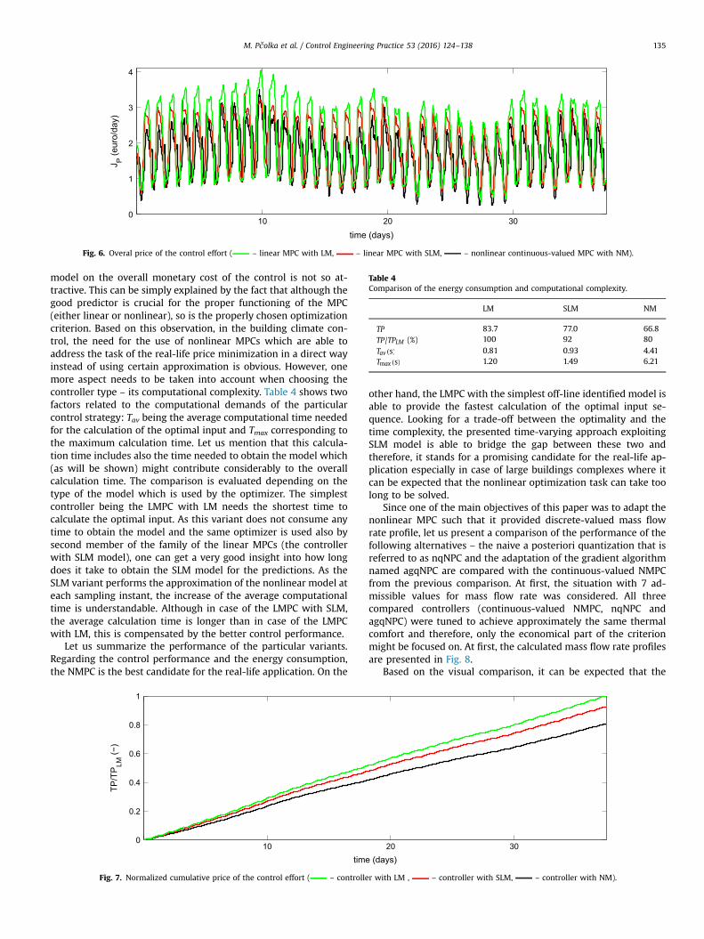
Fig. 6 provides the second part of the visual comparison – itdepicts the monetary cost that is being paid for the control at eachtime instance.

All profiles exhibit sinusoidal-like trends – this is caused by theconsideration of time-varying price of the electricity. The higherparts of the profiles correspond to low-tariff hours while the lowerparts match the non-working hours with cheap electricity. Alsofrom this figure, the monetarily more economical nature of theNMPC can be observed. The NMPC spares significant amount ofexpenses compared to its linear counterparts. This superioritycomes from the use of more precise nonlinear model and it is ofcourse caused also by the nonlinear cost function of the NMPCwhich directly corresponds to the amount of money that is paidfor the control. It can be also seen that the SLM model which iscloser to the nonlinear one enables also the controller with ap-proximated cost function to achieve better economical perfor-mance than the original linear model. For further illustration, thecumulative sum of the monetary cost of the control is depicted inFig. 7. The provided profiles are normalized with respect to thetotal price TPLM that is paid by the linear MPC with the ordinarytime-invariant linear model.

The statistical comparison of the energy consumption can befound in Table 4. TP expresses the overall price paid for zonetemperature control. Moreover, the particular energy consump-tions normalized with respect to the consumption of the linearMPC using the ordinary off-line identified linear model are ex-pressed. Furthermore, also the comparison of the average com-putational time Tav and the maximum computational time Tmax

per discrete time instance is provided.The superiority of the NMPC is demonstrated once again. It can

be seen that although the comparison of the identified models wasvery optimistic in the case of linear time-dependent model versusthe linear time-invariant one, the resulting effect of the good

3 4 5e (h)

with SLM, – nonlinear continuous-valued MPC with NM, – TZmin).

10 20 300

1

2

3

4

time (days)

J P (e

uro/

day)

Fig. 6. Overal price of the control effort ( – linear MPC with LM, – linear MPC with SLM, – nonlinear continuous-valued MPC with NM).

Table 4Comparison of the energy consumption and computational complexity.

LM SLM NM

TP 83.7 77.0 66.8TP TP/ LM (%) 100 92 80

( )T sav 0.81 0.93 4.41( )T smax 1.20 1.49 6.21

M. Pčolka et al. / Control Engineering Practice 53 (2016) 124–138 135

model on the overall monetary cost of the control is not so at-tractive. This can be simply explained by the fact that although thegood predictor is crucial for the proper functioning of the MPC(either linear or nonlinear), so is the properly chosen optimizationcriterion. Based on this observation, in the building climate con-trol, the need for the use of nonlinear MPCs which are able toaddress the task of the real-life price minimization in a direct wayinstead of using certain approximation is obvious. However, onemore aspect needs to be taken into account when choosing thecontroller type – its computational complexity. Table 4 shows twofactors related to the computational demands of the particularcontrol strategy: Tav being the average computational time neededfor the calculation of the optimal input and Tmax corresponding tothe maximum calculation time. Let us mention that this calcula-tion time includes also the time needed to obtain the model which(as will be shown) might contribute considerably to the overallcalculation time. The comparison is evaluated depending on thetype of the model which is used by the optimizer. The simplestcontroller being the LMPC with LM needs the shortest time tocalculate the optimal input. As this variant does not consume anytime to obtain the model and the same optimizer is used also bysecond member of the family of the linear MPCs (the controllerwith SLM model), one can get a very good insight into how longdoes it take to obtain the SLM model for the predictions. As theSLM variant performs the approximation of the nonlinear model ateach sampling instant, the increase of the average computationaltime is understandable. Although in case of the LMPC with SLM,the average calculation time is longer than in case of the LMPCwith LM, this is compensated by the better control performance.

Let us summarize the performance of the particular variants.Regarding the control performance and the energy consumption,the NMPC is the best candidate for the real-life application. On the

100

0.2

0.4

0.6

0.8

1

time

TP/T

PLM

(−)

Fig. 7. Normalized cumulative price of the control effort ( – controlle

other hand, the LMPC with the simplest off-line identified model isable to provide the fastest calculation of the optimal input se-quence. Looking for a trade-off between the optimality and thetime complexity, the presented time-varying approach exploitingSLM model is able to bridge the gap between these two andtherefore, it stands for a promising candidate for the real-life ap-plication especially in case of large buildings complexes where itcan be expected that the nonlinear optimization task can take toolong to be solved.

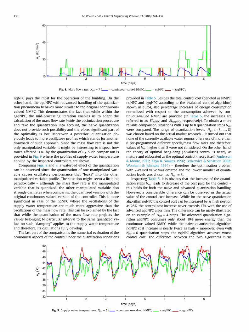
Since one of the main objectives of this paper was to adapt thenonlinear MPC such that it provided discrete-valued mass flowrate profile, let us present a comparison of the performance of thefollowing alternatives – the naive a posteriori quantization that isreferred to as nqNPC and the adaptation of the gradient algorithmnamed agqNPC are compared with the continuous-valued NMPCfrom the previous comparison. At first, the situation with 7 ad-missible values for mass flow rate was considered. All threecompared controllers (continuous-valued NMPC, nqNPC andagqNPC) were tuned to achieve approximately the same thermalcomfort and therefore, only the economical part of the criterionmight be focused on. At first, the calculated mass flow rate profilesare presented in Fig. 8.

Based on the visual comparison, it can be expected that the

20 30 (days)

r with LM , – controller with SLM, – controller with NM).

1 2 3 4 5 6 7 815

30

45

60

time (days)

u 2 (kg/

hm2 )

Fig. 8. Mass flow rates, =N 7qst ( – continuous-valued NMPC, – nqNPC, – agqNPC).

M. Pčolka et al. / Control Engineering Practice 53 (2016) 124–138136

nqNPC pays the most for the operation of the building. On theother hand, the agqNPC with advanced handling of the quantiza-tion phenomena behaves more similar to the original continuous-valued NMPC. This demonstrates the fact that while within theagqNPC, the mid-processing iteration enables us to adapt thecalculation of the mass flow rate inside the optimization procedureand take the quantization into account, the naive quantizationdoes not provide such possibility and therefore, significant part ofthe optimality is lost. Moreover, a posteriori quantization ob-viously leads to more oscillatory profiles which stands for anotherdrawback of such approach. Since the mass flow rate is not theonly manipulated variable, it might be interesting to inspect howmuch affected is u1 by the quantization of u2. Such comparison isprovided in Fig. 9 where the profiles of supply water temperatureapplied by the inspected controllers are shown.

Comparing Figs. 8 and 9, a waterbed effect of the quantizationcan be observed since the quantization of one manipulated vari-able causes oscillatory performance that “leaks” into the othermanipulated variable profile. The situation might seem a little bitparadoxically – although the mass flow rate is the manipulatedvariable that is quantized, the other manipulated variable alsostrongly oscillates when comparing the quantized version with theoriginal continuous-valued version of the controller. This is moresignificant in case of the nqNPC where the oscillations of thesupply water temperature are much more aggressive than theoscillations of the mass flow rate. This can be explained by the factthat while the quantization of the mass flow rate projects thevalues belonging to particular interval to the same quantized va-lue, no such “damping” applies to the supply water temperatureand therefore, its oscillations fully develop.

The last part of the comparison is the numerical evaluation of theeconomical aspects of the control under the quantization conditions

1 2 3 432

34

36

38

40

42

44

46

48

50

time

u 1 (°C

)

Fig. 9. Supply water temperatures, =N 7qst ( – conti

provided in Table 5. Besides the total control cost (denoted as NMPC,nqNPC and agqNPC according to the evaluated control algorithm)shown in euros, also percentage increases of energy consumptionnormalized with respect to the consumption achieved by con-tinuous-valued NMPC are provided (in Table 5, the increases arereferred to as EInqNPC and EIagqNPC, respectively). To obtain a morereliable comparison, situations with 3 up to 8 quantization steps Nqst

were compared. The range of quantization levels ∈ { … }N 3, , 8qst

was chosen based on the actual market research – it turned out thatnone of the currently available water pumps offers use of more than8 pre-programmed different speeds/mass flow rates and therefore,values of Nqst higher than 8 were not considered. On the other hand,the theory of optimal bang-bang (2-valued) control is nearly asmature and elaborated as the optimal control theory itself (Anderson& Moore, 1971; Kaya & Noakes, 1996; Ledzewicz & Schättler, 2002;Wonham & Johnson, 1964) – therefore the optimization problemwith 2-valued valve was omitted and the lowest number of quanti-zation levels was chosen as =N 3qst .

Inspecting Table 5, it is obvious that the increase of the quanti-zation steps Nqst leads to decrease of the cost paid for the control –this holds for both the naive and advanced quantization handling.However, a considerable difference can be observed in the actualvalue of the control cost increase. While for the naive quantizationalgorithm nqNPC the control cost can be increased by as high portionas 28%, the control cost increase never exceeds 17% with the use ofadvanced agqNPC algorithm. The difference can be nicely illustratedon an example of =N 4qst steps. The advanced quantization algo-rithm agqNPC consumes only about 10% more energy than thecontinuous-valued NMPC while the naive quantization algorithmnqNPC cost increase is nearly twice as high – moreover, even with

=N 6qst quantization steps, the nqNPC algorithm achieves worsecontrol cost. The difference between the two algorithms turns

5 6 7 8

(days)

nuous-valued NMPC, – nqNPC, – agqNPC).

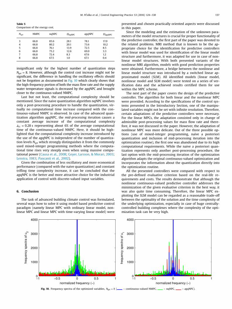
Table 5Comparison of the energy cost.

Nqst NMPC nqNPC EInqNPC agqNPC EIagqNPC

3 66.8 85.6 28.1 78.1 17.04 66.8 80.2 20.1 73.6 10.25 66.8 76.1 13.9 72.5 8.56 66.8 75.2 12.6 69.0 3.37 66.8 72.4 8.3 67.6 1.28 66.8 67.5 1.0 67.1 0.4

M. Pčolka et al. / Control Engineering Practice 53 (2016) 124–138 137

insignificant only for the highest number of quantization steps=N 8qst . However, although the control cost increase might not be

significant, the difference in handling the oscillatory effects shouldnot be forgotten as documented in Fig. 10 which clearly shows thatthe high-frequency portion of both the mass flow rate and the supplywater temperature signals is decreased by the agqNPC and broughtcloser to the continuous-valued NMPC.

Last but not least, the computational complexity should bementioned. Since the naive quantization algorithm nqNPC involvesonly a post-processing procedure to handle the quantization, vir-tually no computational time increase compared with the con-tinuous-valued NMPC is observed. In case of the advanced quan-tization algorithm agqNPC, the mid-processing iteration causes aconstant average increase of the computational complexityΔ = 0.28 sct representing about 6% of the average computationaltime of the continuous-valued NMPC. Here, it should be high-lighted that the computational complexity increase introduced bythe use of the agqNPC is independent of the number of quantiza-tion levels Nqst which strongly distinguishes it from the commonlyused mixed-integer programming methods where the computa-tional time rises very steeply even when using massive compu-tational power (Causa et al., 2008; Geyer, Larsson, & Morari, 2003;Lenstra, 1983; Pancanti et al., 2002).

Given the combination of less oscillatory and more economicalperformance (compared with the naive quantization) and constanttrifling time complexity increase, it can be concluded that theagqNPC is the better and more attractive choice for the industrialapplication of control with discrete-valued input variables.

6. Conclusion

The task of advanced building climate control was formulated,several ways how to solve it using model based predictive controlparadigm (namely linear MPC with ordinary linear model, non-linear MPC and linear MPC with time-varying linear model) were

Fig. 10. Frequency spectra of the optimized variables, =N 8qst (

presented and chosen practically oriented aspects were discussedin this paper.

Since the modeling and the estimation of the unknown para-meters of the model structures is crucial for proper functionality ofthe predictive controller, the first part of the paper was devoted tothe related problems. MRI method that is known to be the ap-propriate choice for the identification for predictive controllerswith linear model was used for identification of the linear modelstructure and furthermore, it was adapted for use in case of non-linear model structures. With both presented variants of thenonlinear MRI algorithm, models with good prediction propertieswere obtained. Furthermore, a bridge between the nonlinear andlinear model structure was introduced by a switched linear ap-proximated model (SLM). All identified models (linear model,nonlinear model and SLM model) were tested on a series of ver-ification data and the achieved results certified them for usewithin the MPC scheme.

The next part of the paper covers the design of the predictivecontroller. The algorithm for both linear and the nonlinear MPCwere provided. According to the specifications of the control sys-tems presented in the Introductory Section, one of the manipu-lated variables might not be set with infinite resolution. Therefore,certain adaptations of the predictive controllers were necessary.For the linear MPCs, the adaptation consisted only in change ofadmissible post-processing values for mass flow rate and there-fore, it was not discussed in the paper. However, the adaptation ofnonlinear MPC was more delicate. Out of the three possible op-tions (use of mixed-integer programming, naive a posterioriquantization and inclusion of mid-processing iteration into theoptimization routine), the first one was abandoned due to its highcomputational requirements. While the naive a posteriori quan-tization represents only another post-processing procedure, thelast option with the mid-processing iteration of the optimizationalgorithm adapts the original continuous-valued optimization andincorporates the information about the quantization directly intothe optimization routine.

All the presented controllers were compared with respect tothe pre-defined evaluative criterion based on the real-life re-quirements and costs. The results demonstrate that although thenonlinear continuous-valued predictive controller addresses theminimization of the given evaluative criterion in the best way, itwas also quite time consuming. Therefore, the linear MPC ex-ploiting the SLM model can be regarded as a reasonable trade-offbetween the optimality of the solution and the time complexity ofthe underlying optimization, especially in case of huge centrally-controlled building complexes where the complexity of the opti-mization task can be very high.

– continuous-valued NMPC, – nqNPC, – agqNPC).

M. Pčolka et al. / Control Engineering Practice 53 (2016) 124–138138

The other part of the comparison was focused on evaluation ofthe performance of the nonlinear controllers under the restrictionson the discrete-valued nature of the mass flow rate. The providedcomparison shows that the advanced of the inspected methodsagqNPC is not only able to keep the economical aspects of thecontrol closer to standard of the original continuous-valued con-trollers but also helps us to reduce the oscillations of the ma-nipulated variables for the cost of a negligible constant timecomplexity increase. Therefore, it can be suggested that the ad-vanced agqNPC algorithm be used in practice instead of naive butcommonly frequently used a posteriori quantization.

Regarding the future work, it would be interesting to examinethe effect of incorporation of the persistent excitation conditioninto the predictive controller procedure. Based on the availableliterature, if the persistent excitation condition is included, moreinformative data are obtained which then turns into a betterability to estimate the model parameters accurately. The suggestedprocedure should be compared with the advanced Kalman filter-ing algorithms such as Extended or Unscented Kalman filtering.Moreover, a procedure for the model parameter update should bedesigned for the nonlinear model. Last but not least, based on theperformed numerical experiments the authors suggest the stra-tegies be tested on a building in real operation.

Acknowledgment

This research has been supported by the Czech Science Foun-dation through the Grant nos. 13-20433S and 13-12726J.

References

Anderson, B. D. & Moore, J. B. (1971). Linear optimal control (Vol. 197). EnglewoodCliffs: Prentice-Hall.

ASHRAE. (2009). ASHRAE-handbook fundamentals. NE Atlanta, GA: American societyof heating, refrigerating and air-conditioning engineers, Inc.

Balmer, R. T. (2010). Modern engineering thermodynamics-textbook with tablesbooklet. Academic Press, Oxford, UK.

Barták, M. (2010). Úvod do přenosových jevu pro inteligentní budovy. Prague, CzechRepublic: CTU Prague.

Bryson, A. E., & Ho, Y. C. (1975). Applied optimal control: optimization, estimation, andcontrol. Taylor and Francis, Oxford, UK.

Bussieck, M. R. & Vigerske, S. (2010). MINLP solver software. InWiley encyclopedia ofoperations research and management science.

Causa, J., Karer, G., Núnez, A., Sáez, D., Škrjanc, I., & Zupančič, B. (2008). Hybrid fuzzypredictive control based on genetic algorithms for the temperature control of abatch reactor. Computers & Chemical Engineering, 32(12), 3254–3263.

Chi, Q., Fei, Z., Zhao, Z., Zhao, L., & Liang, J. (2014). A model predictive control ap-proach with relevant identification in dynamic PLS framework. Control En-gineering Practice, 22, 181–193.

European Economic and Social Committee. (2005). S.M. act: Communication fromthe commission to the council, The European parliament, The European eco-nomic and social committee and the committee of the regions.

Falcone, P., Borrelli, F., Tseng, H. E., Asgari, J., & Hrovat, D. (2008). Linear time-varying model predictive control and its application to active steering systems:Stability analysis and experimental validation. International Journal of Robust andNonlinear Control, 18(8).

Geyer, T., Larsson, M., & Morari, M. (2003). Hybrid emergency voltage control inpower systems. In Proceedings of the European control conference, 2003.

Gopaluni, R., Patwardhan, R., & Shah, S. (2004). MPC relevant identification—Tuning

the noise model. Journal of Process Control, 14(6), 699–714.Gyalistras, D., & Gwerder, M. (2010). Use of weather and occupancy forecasts for

optimal building climate control (OptiControl): Two years progress report.Terrestrial Systems Ecology ETH Zurich, Switzerland and Building TechnologiesDivision, Siemens Switzerland Ltd., Zug, Switzerland.

Kaya, C. Y., & Noakes, J. L. (1996). Computations and time-optimal controls. OptimalControl Applications and Methods, 17(3), 171–185.

Laurí, D., Salcedo, J., Garcia-Nieto, S., & Martínez, M. (2010). Model predictivecontrol relevant identification: Multiple input multiple output against multipleinput single output. Control Theory & Applications, IET, 4(9).

Ledzewicz, U., & Schättler, H. (2002). Optimal bang–bang controls for a two-com-partment model in cancer chemotherapy. Journal of Optimization Theory andApplications, 114(3), 609–637.

Lenstra, H. W., Jr. (1983). Integer programming with a fixed number of variables.Mathematics of Operations Research, 8(4), 538–548.

Lienhard, J. H. (2013). A heat transfer textbook. Courier Corporation, Cambridge,Massachusetts, USA.

Ljung, L. (1999). System identification. Wiley Online Library.Ljung, L. (2007). System identification toolbox for use with {MATLAB}.Ma, J., Qin, S. J., Li, B., & Salsbury, T. (2011). Economic model predictive control for

building energy systems. In 2011 IEEE PES innovative smart grid technologies(ISGT) (pp. 1–6). IEEE, Piscataway, NJ, USA.

Ma, Y., Kelman, A., Daly, A., & Borrelli, F. (2012). Predictive control for energy effi-cient buildings with thermal storage: Modeling, stimulation, and experiments.IEEE Control Systems, Magazine, 32(1), 44–64.

Oldewurtel, F., Gyalistras, D., Gwerder, M., Jones, C., Parisio, A., Stauch, V., et al.(2010). Increasing energy efficiency in building climate control using weatherforecasts and model predictive control. In 10th REHVA world congress clima (pp.9–12).

Pancanti, S., Leonardi, L., Pallottino, L., & Bicchi, A. (2002). Optimal control ofquantized input systems. In Hybrid systems: computation and control (pp. 351–363). Springer, Berlin Heidelberg, Germany.

Perez-Lombard, L., Ortiz, J., & Pout, C. (2008). A review on buildings energy con-sumption information. Energy and Buildings, 40(3), 394–398.

Prívara, S., Široký, J., Ferkl, L., & Cigler, J. (2011). Model predictive control of abuilding heating system: The first experience. Energy and Buildings, 43(2),564–572.

Pčolka, M., Žáčeková, E., Robinett, R., Čelikovský, S., & Šebek, M. (2014). Economicalnonlinear model predictive control for building climate control. In Americancontrol conference (ACC), 2014 (pp. 418–423). IEEE, Piscataway, NJ, USA.

Pčolka, M., Žáčeková, E., Robinett, R., Čelikovský, S., & Šebek, M. (2014). From linearto nonlinear model predictive control of a building. In IFAC world congress 2014(Vol. 19, pp. 587–592).

R.O. for Network Industries. (2011). Approved electricity tariffs for the householdconsumers for 2011 (online). ⟨http://www.urso.gov.sk/doc/dokumenty/PorovnanieMaxCienEEpreDomacnisti2011.pdf⟩, accessed: 03/11/2013.

Shook, D. S., Mohtadi, C., & Shah, S. L. (1991). Identification for long-range pre-dictive control. In IEEE proceedings D (Control theory and applications) (Vol. 138,pp. 75–84). IET, Piscataway, NJ, USA.

Stetter, H. J. (1973). Analysis of discretization methods for ordinary differential equa-tions (Vol. 23). Springer, Berlin Heidelberg, Germany.

University of Wisconsin-Madison, Solar Energy Laboratory, & Klein, S. A. (1979).TRNSYS, a transient system simulation program. Solar Energy Laboratory, Uni-versity of Wisconsin–Madison.

Verhelst, C., Degrauwe, D., Logist, F., Van-Impe, J., & Helsen, L. (2012). Multi-ob-jective optimal control of an air-to-water heat pump for residential heating.Building Simulation, 5, 281–291.

Wonham, W. M., & Johnson, C. (1964). Optimal bang–bang control with quadraticperformance index. Journal of Fluids Engineering, 86(1), 107–115.

Žáčeková, E., & Prívara, S. (2012). Control relevant identification and predictivecontrol of a building. In 2012 24th Chinese control and decision conference (CCDC)(pp. 246–251). IEEE, Piscataway, NJ, USA.

Žáčeková, E., Váňa, Z., & Cigler, J. (2014). Towards the real-life implementation ofMPC for an office building: Identification issues. Applied Energy, 135, 53–62.

Zhao, J., Zhu, Y., & Patwardhan, R. (2014). Some notes on MPC relevant identifica-tion. In American control conference (ACC), 2014 (pp. 3680–3685). IEEE,Piscataway, NJ, USA.

Zhou, K., Doyle, J. C., Glover, K., (1996). Robust and optimal control (Vol. 40). NewJersey: Prentice Hall, Upper Saddle River, New Jersey, USA.

Zmrhal, V., & Drkal, F. (2006). The influence of heat convection on room air tem-perature. In Proceedings of 17th air-conditioning and ventilation conference.