control based sensor management for a multiple radar ...kokar/publications/sensormgmntif04.pdf ·...
TRANSCRIPT

Control Based Sensor Management
for a Multiple Radar Monitoring Scenario
Yong Xun and Mieczyslaw M. KokarDepartment of Electrical and Computer Engineering
Northeastern University, Boston, Massachusetts
[email protected] and [email protected]
Kenneth BaclawskiCollege of Computer Science
Northeastern University, Boston, Massachusetts
Abstract
In this paper we consider the problem of monitoring illuminations of multipleemitters by one electronic receiver located on a moving platform. The emittersexhibit a quasi-periodic radiation pattern, each in a different frequency band andwith a different illumination period and illumination time. The goal is to tunethe receiver to the appropriate frequency band at the appropriate time so as tomaximize the probability of detection of each illumination of each radar (expressedas a quality of service metric). This problem can be viewed as two subproblems:(1) generating tuning requests by particular frequency bands and (2) scheduling thereceiver to satisfy the requests. In our scenario the number of requests from all thebands exceeds the physical capability of one receiver (overload) and thus selectionis needed. The goal is to push the limits on the overload while still maintaininga required level of quality of service metric. This can be achieved by controllingboth the generation of the tuning requests and the scheduling. According to thecontrol theory metaphor of software development, we map this problem onto acontrol architecture with one system-level controller and a collection of emitter-level controllers (one per emitter). We show that our control based sensor managerhas significant advantages over a scheduler without feedback in terms of both theoverload and the quality of service metric. We also discuss design issues of suchsensor management systems.
Keywords: multiple radar monitoring, real-time task generation, real-time scheduling,
real-time resource allocation, sensor scheduling, sensor management
1

1 Introduction
Modern avionics systems carry a number of sensors for collecting data about the environ-
ment. Normally the demands for sensing are much higher than the physical capabilities
that the sensors can provide. As a consequence, the sensors must be used selectively,
balancing the conflicting sensing requests from the point of view of the goal of the mis-
sion of the avionics system. The research domain that deals with scheduling sensors is
called Sensor Management. According to [1], the goal of a sensor management system
is to “select the right sensor to perform the right service on the right object at the right
time”.
In this paper we consider the problem of managing sensors that monitor sources of
electronic radiation in the environment (such as radars). The sources emit radiation in
different frequencies and with various illumination patterns and periodicities. The goal is
to detect each illumination of each emitter. In other words, the goal is one of monitoring
all the emitters and not just detecting active radars. Information about each illumination
of a radar can be used by on-board electronics for countermeasures like deception and
jamming.
In our scenario an omni-directional receiver is tuned to a particular frequency band
to detect a radar emitting in this frequency band. Since we assume that the emitters
operate independently of each other, each frequency band can be treated as a virtual
sensor, each with its own sensing needs. The sensing needs of one sensor can conflict
with other sensors, since more than one sensor can request the same resource at the same
time. However, since we have only one receiver, only one of the sensors can be active
at any specific time. Therefore, the requests for tuning to particular frequency bands
must be scheduled appropriately, so that the receiver is sensing at the time when the
illumination occurs.
Because of the large number of actual and potential emitters in an environment,
it is important to minimize the time spent attempting to observe each emitter, while
also maximizing the probability of detecting each illumination by an emitter. It is also
2

important to keep frequency bands available for other uses, such as jamming. This
results in additional pressure to reduce the time scheduled for the sensors to perform
observations in each frequency band.
The problem considered in this paper is a great simplification (an abstraction) of real
applications of this kind. However, since this is a non-preemptive scheduling problem,
which is known to be NP-complete [2], a full and complete algorithmic solution to this
problem does not exist. Consequently, algorithms that can push the limits in terms of
the quality of solutions of this problem are sought. Moreover, this kind of scenario is
of interest to other domains. For instance, a similar kind of problem is manifest in the
managing of streaming media, which has similar characteristics.
A generally agreed upon model for sensor management (cf. [1]) is to view it as a loop
consisting of three major functions: generate options, prioritize options and schedule
tasks. The first function generates requests for sensor tasks, the second assigns priorities
to the tasks, and the third then assigns the time of execution to each task. In this paper we
consider all three functions. Options are generated separately for each sensor (frequency
band). Priorities for tasks are assigned dynamically; the Quality of Service metric defined
in the paper is used for this purpose. Note that the term “priority” refers here to a metric
that the scheduler uses in selecting tasks for execution and not to the priority of a given
emitter to the mission. The scheduler then fuses the information from all the virtual
sensors and makes a decision on which sensor to schedule. Since in the subject domain
the solution to this sensor management problem is termed as “scheduling”, in the rest
of this paper we use this term to mean inclusively “option generation, prioritization and
scheduling”.
The environment that we deal with is highly dynamic. Emitters are rotating and
the receiver is located on a moving platform. In the general case, emitters can move,
and illumination patterns can vary over time. Furthermore, events can occur over a very
large range of time scales. Individual radiation pulses may be as brief as a nanosecond,
while illumination periodicities can be as long as several seconds. More details about
the scenario used in this study are given in Section 2. Additionally, since the scheduler
3

is decoupled from the task generation and prioritization functions, the scheduler may
introduce delays in scheduling the sensors (cf. [3]).
To compensate for the dynamics of the environment and of the system, we build and
use a resource manager based on the control theory metaphor of software development
[4]; we call this manager Dynamic Scan Scheduler (DSS). We formalize the dynamics of
this resource allocation problem in Section 5.2. In order to map the problem onto the
control architecture, we must also have a well defined quality of service (QoS) metric
that can be used both to specify the required level of service and to measure the actual
level of service achieved. The QoS metric used in our study is discussed in Section 5.3.
The next step is to choose a suitable control architecture and controllers. Our method-
ology is based on a general architecture for self-controlling software [4] which is special-
ized to this particular resource management problem. In this case, we chose a two-level
feedback control architecture. We discuss our rationale for this choice in Section 5.1.
Finally, we evaluate our solution and compare it with other approaches used to solve
this particular problem. The results of our simulations and comparisons are presented in
Section 6. One approach is to develop a schedule off-line in advance of a mission. This
type of resource manager, called a fixed scan scheduler (FSS), is introduced in Section 3.
An algorithm for constructing fixed scan schedules is presented, and some examples are
given. This technique guarantees detection of each illumination for low loads, i.e., when
the number of emitters in the environment is small. This technique does not provide
graceful degradation when the load becomes high.
We also consider another technique, periodic dynamic scheduling, that relies on prior
knowledge about the frequency of illumination of the emitters. This technique is intro-
duced in Section 4. This technique is dynamic but not adaptive. We show that the
control based scheduler outperforms both of the other approaches. Furthermore, our
solution uses only about 10% of the observation time as the fixed scan schedule, and
our solution does not depend as much on the prior knowledge about the emitters as the
periodic dynamic scheduling technique. The main reason for the performance advantages
4

of our solution is that neither of the other two schedulers can adapt to dynamic changes
in the environment. In our scenario, from the point of view of the receiver, the emitters
are only quasi-periodic (due to the motion of the platform) and thus the sensor manager
must compensate for the phase shift in illumination due to the motion. We end the paper
in Section 7 with our conclusions and an outline of future research directions.
Sensor management has been formulated as an optimization problem in [5]. Since then
various attempts have been made both to refine the formulation and to solve this problem.
One of the directions was to use information theory based performance metrics [6, 7].
However, Musick and Malhotra [1] state that “decision theoretic methods do not directly
support scheduling”. Another way to approach this problem is to treat it as a Dynamic
Programming problem (cf. [1]). However, as stated in [1], “dynamic programming does
not begin to resolve the modeling complexities innate in Sensor Management”. Moreover,
in our scenario we cannot even assume that we know the state transition function and
thus estimation of the future states is necessary. When combined with the requirement
of non-preemption of scheduling, this formulation does not solve our problem (one of the
reasons being the NP-completeness of non-preemptive scheduling mentioned above).
Control techniques have also been applied to sensor management in various ways,
e.g., [3, 6], but mainly for scenarios where the goal was to manage sensors used for
tracking moving objects. One of the distinguishing features of our scenario is that our
system has discrete input (detection or non-detection). Although similarly as in [3] in
our scenario we also have an architecture in which the scheduling function is separated
from the option generation function, and thus we have a similar problem with the delays
due to this architecture, we could not apply these results to our scenario mainly because
these results are related to tracking, rather than detection.
Feedback and control based algorithms have also been used in the area of real-time
systems, where there is a need for scheduling the processor for computational tasks
(cf. [8, 9, 10, 11]). This work, however, addresses only one of the problems of sensor
management, i.e., the scheduling part.
5

2 Scenario and Notation
In this section we describe the simulated scenario in more detail, especially the simplifying
assumptions we made, and introduce some notation used throughout the paper.
In Figure 1 we show a typical emitter illumination pattern. The radiation is produced
in short pulses. These, in turn, form batches called illuminations. The pulses are shown
here as square pulses, but the actual pulses are high frequency waveforms. The line over
each illumination group is meant to represent the envelope of the illumination. It is not
another signal.
Figure 1: Signal
While the pulses are produced electronically, we assume that the illuminations are
the result of the mechanical motion of the radar antenna. This has some important
consequences. The time between pulses can be very short and can be very regular. On
the other hand, the time between successive illuminations is typically much longer and
need not be as regular. These assumptions are not valid for other types of emitter, for
instance for phased array antennas, where any illumination pattern is possible. We do
not consider this kind of emitters in our scenario.
The most important emitter parameters are the following: fe - the frequency of the
emitter’s signal (waveform); Ae - signal strength (power level) of the emitter; Tpri - Pulse
Repetition Interval (PRI) of the emitter (time between successive pulses within a single
illumination); Tpw - pulse width (PW) of the emitter; Teip - the illumination period (time
between successive illuminations, determined by the rotation period of the radar); Be -
beam width of the emitter (angle scope within which the emitter is radiating at a given
6

time, determines the angle within which a target can be detected); Teit - illumination
time (duration of a single illumination); τe - the minimum time required for a detection
of the emitter against background noise.
We assume that the kinds of emitter (radar) that might be encountered during a
mission are known in advance. In particular, we assume that the radar monitoring
system has basic data on the frequencies used by the emitters and the times between
successive illuminations when the emitters are operating. Obviously, we do not assume
that the phases for particular radars are known.
Another simplifying assumption is that the monitoring system can recognize the type
of radar by its pulse pattern. This is not necessarily true in more complex and realistic
scenarios. Nevertheless, in our scenario we assume that when an emitter has been de-
tected, an attempt is made to identify the kind of emitter from a database of potential
emitters. If this is successful, then the entry in the database is transferred to a table
called the Active Emitter Table (AET). The AET is the primary output of the sensor,
and it can also be used for scheduling the sensor. If the emitter cannot be identified as
a known kind of emitter, then the system creates a new AET entry as well as a new
database entry. This usually requires that the emitter be detected more than once in
order to obtain an estimate for the illumination period.
Although we do not assume that there is at most one radar operating in each fre-
quency band, we do assume that radars operating in the same frequency band can be
distinguished from one another. The fact that this sensor operates in the same frequency
band as another sensor does not make too much of a difference to the monitoring system.
As we already said in Section 1, even though this scenario is a great oversimplification
of any realistic scenario, due to the fact that this is a case of non-preemptive scheduling,
which is known to be NP-complete [2], it is worthwhile searching for algorithms that per-
form better in specific conditions. In our case the distinguishing conditions are that the
goal is to detect each illumination of multiple emitters and that the system is operating
under relatively high overload.
7

2.1 Tasks and Schedules
Requests for tuning the receiver to the frequency band of a given emitter are called tasks.
Each task is represented by a Control Description Word (CDW). A CDW specifies when
and for how long the receiver is to be tuned to a particular frequency band. Each CDW
is a request for a single dwell of the receiver. Mathematically, a CDW is a triple:
CDW = (tds, τd, ω) (1)
where tds is the time when the dwell should begin and τd is the length of time that the
receiver devotes to this dwell. A scan schedule (SS) is a sequence of CDWs, one per
dwell:
SS = CDW1, CDW2, ..., CDWn (2)
A scan schedule is simply the sequence of commands given to a receiver. Within a scan
schedule, one can define the notion of the revisit time, τrv, the time from the beginning
of the last dwell until the beginning of the next dwell on a particular frequency band.
From the beginning time of the last dwell and the revisit time, one can compute the start
time of the next dwell.
The most basic constraint that a schedule must satisfy is called the capacity constraint.
This constraint simply states in mathematical form the fact that a receiver can only be
tuned to one frequency band at a time. For the virtual sensors it means that only
one sensor can be scheduled at a time. For a scan schedule for which the number of
frequency bands is a fixed number N and for which the dwell time and revisit time for
each frequency band i is fixed, the capacity constraint is:
W =N∑
i=1
τd(i)
τrv(i)≤ 1 (3)
The quantity W is called the workload. Another way to view the capacity constraint
is to introduce the notion of the duty cycle; it is the fraction of the time allocated to
this emitter. More precisely, it is the ratio of the dwell time to the revisit time for this
emitter. The capacity constraint states that the total of all duty cycles can be no larger
than 1.
8
The satisfaction of the capacity constraint is not sufficient to ensure that a scan
schedule exists. This is because the revisit times of different frequency bands may cause
scheduling conflicts: two or more frequency bands may request the receiver at the same
time. For this reason scheduling is an important part of the sensor control.
3 Fixed Scan Scheduling
One of the techniques of monitoring all illuminations of radars is the Fixed Scan Schedul-
ing technique. A fixed scan schedule consists of a fixed sequence of CDWs for the entire
mission of the platform. In this sequence, the CDWs for a specific emitter differ only in
the start time tds, i.e., all the dwell times τd and the revisit times τrv for that emitter
are the same. The main idea behind fixed scan scheduling is that in order to guarantee
detection of each illumination, the receiver dwells should be spaced apart by no more
than the illumination time of the emitter. With multiple emitters, this requirement is
difficult to satisfy since multiple emitters might require dwell at the same time.
There are several ways to construct an fixed scan schedule. A rate monotonic fixed
scan scheduler (RM) [12, 13, 14, 15] is a general task scheduling technique that uses
two pieces of data about tasks: task execution time and period. It is a priority-based
scheduling technique which assigns the highest priority to the task with the shortest
period. For sensors, the execution time is the dwell time and the period is the revisit
time. If one assumes that the dwell time is equal to K pulse repetition intervals (where
K is typically equal to 3), then the following equations describe the rate monotonic scan
scheduler:
τd = K · Tpri (4)
τrv = Teit − τd (5)
This assumes that the emitters emit pulses in a uniform pattern. It would not apply
to emitters that use a non-uniform pattern, such as radars that employ a stagger pattern
9

in which a non-periodic pattern of pulses is emitted repeatedly.
Figure 2 is an example of a rate-monotonic schedule. This schedule includes four
emitters (E1, E2, E3, E4). Their characteristics (dwell time, illumination time) are given
by: E1 : (0.5, 4), E2 : (0.3, 6), E3 : (0.8, 8) and E4 : (0.6, 12), respectively. Since RM
scheduling gives higher priority to tasks with shorter periods, the priorities for these four
emitters are 4, 3, 2 and 1, respectively.
Figure 2: Example: A Fixed Scan Schedule
The computation of a rate-monotonic FSS starts by determining the least common
multiple of the revisit times of the emitters. We call this the scheduling cycle. In the
example of Figure 2, the revisit times are 4, 6, 8 and 12, so that the scheduling cycle is
24. In the next step, the CDW for the emitter having the highest priority is specified.
This process is then repeated for the other emitters in order of priority until the scan
schedule has been determined for the entire scheduling cycle. If the capacity constraint
(Equation 3) is violated, then some revisit times must be increased using some rule, such
as increasing the revisit time of lower priority emitters, until a scan schedule satisfies
the capacity constraint and a schedule can be found. The schedule developed for one
scheduling cycle is then repeated for all consecutive cycles.
In the absence of any new information (i.e., in the absence of any emitter detections),
an FSS has reasonably good performance, especially if the scenario is the same as was
anticipated during the selection of a given schedule. A FSS has the advantage that it is
simple and thus easy to implement. This technique is also important because it is usually
the initial schedule for any other kind of scan scheduling.
10
However, FSS is based on prior knowledge about the environment, so it is not ap-
plicable in unknown environments or environments that change. In particular, since it
does not have a feedback mechanism, it cannot adapt to changes in the environment.
Consider, for example, a rate monotonic FSS and a simple scenario consisting of a single
emitter and a single sensor having the following parameters:
Tpri = 2.0 · 10−3 sec (6)
Tpw = 1.5 · 10−5 sec (7)
Teip = 4.0 sec (8)
Be = 2o (9)
From these equations one can calculate the illumination time to be:
Teit = 4.0 sec · (2o/360o) = 0.02 sec (10)
The dwell and revisit times for a rate monotonic fixed scan schedule will then be:
τd = 3 · Tpri = 6.0 · 10−3 sec (11)
τrv = Teit − τd = 0.0162 sec (12)
In a rate-monotonic FSS for this scenario, there are 246 CDWs for this emitter in each
scheduling cycle. This corresponds to a duty cycle of
d = τd/τrv = 0.37 (13)
for just this one emitter. The 246 receiver dwells corresponding to these CDWs will
detect at most two illuminations of the emitter. Thus only two dwells will be effective;
the other 244 will be wasted. When there are tens or even hundreds of emitters in the
environment, this kind of scheduling will not be efficient. The goal is to reduce the
number of CDWs required to detect each emitter, or, equivalently, to reduce the emitter
duty cycles. Note, however, that we cannot lower the duty cycles by enlarging revisit
times, since this might result in non-detections of emitter illuminations.
11

4 Introducing Dynamics to a Scheduler
One way to lower the number of dwells is to synchronize the dwells with the illumination
period of a given emitter, after first detection of that emitter. However, in the dynamic
environment we still are risking missing illuminations due to dynamic effects (phase
shifts). To compensate for the dynamics of the environment, a dynamic scan scheduler
(DSS) is then used. Rather than being a fixed scheduling pattern, a dynamic scan
scheduler is an algorithm that dynamically modifies the scan schedule in response to
detection events.
There are several ways that one can introduce dynamics into a scan scheduler. One
possibility is to use a pre-computed fixed scan schedule until first detection, and then
recompute an it so that the newly detected emitter is only dwelled upon at the predicted
illumination times as specified by the entry in the AET. After recomputation the CDWs
for a detected emitter differ only in the start time tds, i.e., all the dwell times τd for the
frequency band of this emitter are the same. We will call this technique periodic dynamic
scan scheduling. The only difference between this technique and FSS is that detected
emitters will have a much longer revisit time.
While periodic dynamic scan scheduling seems like it solves the problem of resource
allocation in this case, it has some serious disadvantages. The main problem is that
the illuminations of the emitters, as sensed by the receiver, will vary over time for a
variety of reasons. The radar antenna, being a mechanical device, could speed up or
slow down. However, a more significant effect is due to the motion of the aircraft.
As the aircraft moves relative to the emitter, the apparent time between illuminations
changes. For instance, consider an emitter with a 6 sec illumination period (i.e., the
radar antenna rotates by one full cycle in 6 sec). Now suppose that the aircraft is 60,000
feet away from the radar and is moving in a circle around the radar at 1000 feet/sec, in
a direction opposite to the rotation of the radar. In such a case while the radar rotates
by 360 degrees, the aircraft moves by 6,000 feet, which is equivalent to about 6 degrees.
Consequently, the apparent time between illuminations will be shorter by approximately
12

0.1 sec. This might seem like an insignificant shift, but since the shift is much higher
than the illumination time, this shift is actually quite important. In fact, the illumination
time is about 20% of the 0.1 sec shift, which is more than sufficient to cause a detection
failure.
To address the problem of dynamic changes in the environment, we propose a control-
based DSS.
5 Mapping to a Control Architecture
We now show how the sensor scheduling problem can be mapped to a control based
architecture. We first review some background in the control theory metaphor of software
development. A specific mapping to a control theory architecture is then proposed.
5.1 Control-Based Architecture
The problem addressed in this paper appears at first to be an excellent candidate for the
standard control theory based paradigm. In this paradigm the problem is formulated
using a model, an optimal control law is derived using control theory and the system
is proved to be stable. Unfortunately, this approach is not possible for the problem
addressed in this paper for various reasons. First, like nearly all nontrivial software
systems, this system is far too complex for a complete mathematical model. Second, the
system is a hybrid system (i.e., it includes both continuous and discrete components).
Finally, the system is nonlinear. Consequently, although formulation of the problem
with a mathematical model and derivation of an optimal control law would be highly
desirable, it is not possible to use the standard control theory methodology in this case.
Faced with such a situation, one is tempted to abandon control theory entirely, and this
is the most common approach. There are many examples of software that incorporates
feedback processing without any reference to control theory at all. The approach used
in this paper is in between these two extremes. We call it the control theory metaphor of
13

software development (see [4]).
The main reason for proposing the control theory metaphor was to address the prob-
lem of changes in software requirements. In the case of embedded software, changes in
software requirements come from changes in the environment with which the software
interacts. As we discussed in Section 3, fixed scan schedules do not perform well when the
environment changes dynamically or the workload is heavy. This is due to the high duty
cycle required for each potential emitter and the relatively low probability of detecting
each emitter. The control theory metaphor seems natural for this kind of application.
The main idea behind the control theory metaphor is to treat the basic software
functionality as a Plant, to treat changes in the environment as disturbances, and to use
feedback from the environment to adjust system behavior. In order to compensate for
disturbances, a Controller must be added. From the point of view of software require-
ments, the Controller is a redundancy that is added to the system. The controller is not
part of the original software requirements. Other kinds of (redundant) modules need to
be added to implement a control loop, as shown in Figure 3.
Figure 3: Control Based Sensor Management Architecture
In the control approach a system consists of two basic elements: a Plant (the system
being controlled) and a Controller. To map a problem to a control architecture, it is
14

necessary to identify a controlled output variable. In a control problem such a variable is
always given explicitly. However, when the original problem statement does not include
such a variable, an appropriate quantity needs to be constructed. The selection of this
quantity is not a trivial task. In our approach we proposed to add a special Quality-of-
Service (QoS) module that assesses the Plant’s output in terms of a Quality-of-Service
measure. The selection of the QoS measure for our problem is discussed in Section 5.3.
5.2 Plant
Referring to Figure 3, the plant for this problem includes a receiver, a sensor management
module and an environment. The receiver is viewed as a number of virtual sensors,
one for each emitter. The sensor management module, similarly as in [1], consists of
three functions: generate options, prioritize and schedule. In our mapping, the first
two functions are included in the module called CDW Generator (task generator). The
scheduling function is obviously included in the Scheduler module. By environment, we
mean the potential emitters. We don’t have any control over the environment and in this
sense this is not quite part of the plant. But, on the other hand, we partially model the
emitters, and then the model is taken into consideration in further analysis. There are
at least two reasons to discuss the model. First, we use the model in the selection of the
controller parameters. Note, however, that it is not a typical derivation of a control law,
like in a standard control-theory approach. Second, the model is used in the simulations
used to evaluate the proposed approach.
5.2.1 Emitters and Receiver
The state of the platform and its receiver at a time t is determined by the position of
the platform and by the frequency band to which the receiver is tuned. The position of
the platform is determined by its Cartesian coordinates (x(t), y(t)) over the terrain. The
altitude of the platform is not significant for this problem domain. The trajectory of the
platform can be arbitrary but it is fixed in a particular mission so it is modeled as the
15

input process of the dynamic system. The position as well as the velocity (x′(t), y′(t)) of
the platform can therefore be regarded as known.
The state of the receiver can be represented by a finite discrete set of frequency bands
(sensors), along with one point representing the state in which the receiver is not tuned
to any band. The current frequency band is written ω, and the set of all such bands
(including the “off” state) is written Ω. The state space for the platform is therefore
the product of the (continuous) two-dimensional plane and the set of frequency bands:
R = IR2 × Ω.
We will assume that the emitters run independently. A state for a single emitter
consists of the following three variables:
1. The direction φ in which the emitter is illuminating its environment. The variable
φ is an angle, and therefore its set of values is isomorphic to the unit circle or to
the half-open interval [0, 2π).
2. The distance r between the platform and the emitter.
3. The angle θ of the platform with respect to the emitter.
The state space for emitter i will be denoted E(i). The variables r and θ represent
the position of the platform with respect to the emitter in polar coordinates. It is
sometimes convenient to use Cartesian coordinates, in which case they will be written
(xe(i, t), ye(i, t)).
Since the emitters were assumed to be independent, the overall state space for the
emitters is the product of the state spaces of the individual emitters∏
i E(i). Combining
this with the state space for the platform, the overall state space for the receiver and the
emitters is:
Q = R × ∏i
E(i) = IR2 × Ω × ∏i
E(i) (14)
16

The evolution function of the system has both continuous and discrete components.
The continuous component evolution is determined by the following stochastic differential
equation for emitter i:d
dtφ(i, t) = 2π/Teip + wφ(i) (15)
d
dtxe(i, t) = x′(t) + wxe(i) (16)
d
dtye(i, t) = y′(t) + wye(i) (17)
In this system of equations, wφ(i), wxe(i) and wye(i) are the noise affecting the respective
derivative. For the radar rotation process the noise wφ(i) is assumed to be Gaussian (with
mean 0). It is also assumed that wφ(i) is independent of the other two noise variables.
The discrete component of the evolution of the receiver is characterized by discon-
tinuous “jumps” from one state to another. The receiver evolution is determined by the
scan schedule. Each CDW that is selected by the scheduler generates an event, which in
turn, causes a discontinuous jump from one frequency band, ωi, to another, ωj, at the
time of the event.
The last component of this dynamic system is the output function. This function
determines what function of the variables of Q are observed as the system evolves. In
this case, the output function computes detections. Whenever the receiver satisfies the
requirements for a detection, the function gives the data associated with the detection.
In the following we define the detection function.
For each emitter i there is an upper limit rm(i) on the distance at which it can be
detected. When the platform is beyond the range of the emitter, then no detection is
possible at any angle. The same would be the case if the emitter were not emitting either
because it was not turned on or because the emitter was not deployed. For the purpose
of this problem, it is not possible to distinguish an out of range emitter from one that is
off.
The following are the requirements for detecting emitter i: the emitter must be
operating and within range, the emitter must be illuminating the receiver, and the emitter
17

frequency must be in the current receiver frequency band. The requirements above must
hold for a period of time at least equal to τe. Putting the conditions above together we
can formally define a detection as follows:
Definition 5.1 Consider a dwell commanded by the CDW = (tds, τd, ω). The time td is
called the time of detection of emitter i, if there exists an interval (t0, td) ⊂ (tds, tds + τd)
such that for every t ∈ (t0, td)
1. r(i, t) < rm(i),
2. |θ(i, t) − φ(i, t)| < Be(i),
3. fe(i) ∈ ω(t), and
4. td − t0 ≥ τe.
The receiver actually measures the amplitude of the illumination continuously during
the dwell time, and it determines that an illumination has occurred by simply comparing
the measured signal with a noise threshold. For this reason the measurement noise will
not be considered in the analysis of the model presented in this paper. A more elaborate
model would, of course, consider the measurement noise in addition to the process noise.
When the receiver dwells on a specific emitter and does not detect that emitter, the
output function returns tl(i), i.e., the time of last look at that emitter. The output
function produces the set of detection times and look times for all emitters.
Definition 5.2 The output function g : T × Ω → T × l, d is a function of time and
frequency bands s.t., g(t, i) = (td, d) if emitter i was detected during last dwell and (tl, l),
if emitter i was not detected during last dwell.
For simplicity, we will say that the value of the function is either td or tl. Since the
value of this function will not change between dwells, the set of detection times will be
denoted as Td and the set of non-detections will be denoted as Tl.
18

Note that this definition assumes that when more than one emitter is transmitting
on the same frequency band, the receiver can distinguish them from each other. In other
words, it can determine which of the potential emitters in a band is actually illuminating
the receiver. Because emitters differ from one another in the detailed structure of the
illumination (i.e., the pulse pattern), this is not an unreasonable assumption, although
it might not always be correct. If such discrimination is not possible, then the output
function must be redefined so that it only computes the frequency band that is being
detected, not the specific set of emitters.
Since a detection can only occur during a dwell, one simplification of the output
function is for the output function to produce a sequence of data structures, one for each
CDW. This is, in fact, what many receivers produce. The output is a data structure
called a pulse descriptor word (PDW) which contains detailed information about the
illumination(s) that were detected during the period of time covered by the CDW.
5.2.2 CDW Generator
Another part of the plant is CDW Generator. We have one CDW generator for each
emitter i ∈ 1, . . . , N. The goal of a CDW Generator is to generate requests for tuning
to the frequency of the specific emitter (tasks), where each such task is represented by
a CDW. Two parts of a CDW, τd and ω, are fixed (cf. Equation 1). So the only value
that may need to be recomputed is the time of the start of the next dwell, tds(i, t + ∆t),
where ∆t is the period of the computation loop (in our simulations it was 10µsec). It is
re-computed at or after the beginning of the current dwell:
t ≥ tds(i, t) (18)
If the emitter illumination were perfectly periodic, if there were no phase shifts, if
both the platform and the emitter were stationary, and if we knew the distance between
the emitter and the platform then we would be able to predict exactly the time of the
next dwell as the time of the current dwell tds(t) plus the revisit time for that receiver
19

τrv:
tds(i, t + ∆t) = tds(t) + τrv(i, t) (19)
In order to compensate for the phase shift, we need to adjust τrv. This is achieved by
using the input from the Emitter-Level Controller, δ(i, t) (see Figure 3). An intuitive
way to achieve this adjustment is to multiply the controller output by the illumination
period of this specific emitter, i.e.,
τrv(i, t) = δ(i, t) · Teip(i) (20)
However, since we use a generic proportional controller, the result of this multiplication
could take the revisit time out of the desired bounds. To avoid this effect, and to add
some nonlinearity (explained later) we replace δ(i, t) in Equation 21 with δ(i, t)2,
τrv(i, t) = δ(i, t)2 · Teip(i) (21)
where δ(i, t) is normalized by the following function:
δ(i, t) =
1, if δ(i, t) > 1√Teit(i)Teip(i)
, if δ(i, t) <√
Teit(i)Teip(i)
δ(i, t), otherwise
(22)
As we can see from this equation, in case the controller output is large, the value of
the revisit time is equal to the illumination period, i.e., the receiver dwells on a given
emitter only once per the illumination period. This kind of situation should occur only
when there was a detection on the previous dwell. When the controller output is small,
the receiver dwells on the emitter after one illumination time. This is then equivalent to
having an FSS sensor manager. Moreover, the normalization function is nonlinear. This
has the effect of generating more CDWs closer to the next expected illumination. An
example of this effect on the sequences of CDWs for a control based DSS is shown in
Figure 4 in Section 5.4.3, where we discuss design issues of such sensor managers. The
figure also shows a pattern of CDWs generated by an FSS. Note that since the CDW
Generator shifts starts of dwells, this module also introduces additional dynamics to the
system.
20

5.2.3 Scheduler
The scheduler is responsible for combining information about all emitters and then ad-
justing the workload and selecting CDWs to be executed by the receiver. The CDWs
generated by the CDW Generators are fed into the scheduler’s queue. However, since
the CDWs are generated by a number of independent generators (one per emitter), there
may be too many CDWs for this receiver to execute. The limit on the capacity of the
receiver is defined by the instant workload; it is violated (i.e, the scheduler is overloaded
[16]) if the value of the workload is higher than one (see Equation 3). In other words, the
set of tasks violates the schedulability constraint [17]. The instant workload is defined as
the sum of the duty cycles of the CDWs in the queue:
W (t) =∑
i∈CDW
τd(i)
τrv(i, t)(23)
where CDW denotes the set of CDWs in the queue. The scheduler adjusts the workload
by adjusting the revisit time for each CDW in the queue as follows:
τ ′rv(i, t) =
τrv(i, t)
c(t)(24)
where c(t) is the coverage parameter computed by the system-level controller. When the
scheduler receives a larger value of c(t) from the system-level controller, the revisit times
of all emitters get smaller (Eq. 24), which results in larger duty cycles, and consequently
in a larger instant workload (Eq. 23).
The scheduler is invoked at schedule time, ts. The schedule time is defined as the
completion time of the current dwell, i.e., tds(t−∆t)+ τd(t−∆t) or the beginning of the
next dwell in the queue. We use a priority-based scheduler, where priorities are based
upon the Quality of Service metric computed dynamically. A scheduling decision ω(ts)
is made based upon the current value of the QoS (which will be defined in Section 5.3),
where a specific frequency band j is chosen if the QoS for it is the largest, i.e.,
ω(ts) = j, (25)
QoS(j, ts) = maxi
QoS(i, ts) (26)
21

5.3 The Quality of Service Metric
The QoS is a metric that determines the level of quality exhibited by the system at any
point in time. It can be used to specify the required level of service of the system and
to compare the performance of different algorithms. As noted in Section 5.2 above, the
purpose of the system is to keep the QoS at a given (low) level. In this section we define
this metric. First, we introduce the emitter-level QoS(i, t) metric (for an emitter i at
time t) and then combine all the emitter-level metrics to obtain a system-level metric
QoS(t).
The goal of this sensor system is to detect each illumination of each radar. The success
of this operation depends on the knowledge of one of the state variables of each emitter,
the beam direction of the emitter. Therefore, we want the QoS function to measure
the accuracy of the estimates of this state variable. Since the dynamic system for each
emitter is a linear stochastic dynamic system (cf. Section 5.2.1), the overall measure of
accuracy is the (co)variance of the error estimates.
The rotation of the emitter, which is a mechanical system, is subject to mechanical
noise. The noise term is written wφ(i) in Equation 15. We assume that wφ(i) is indepen-
dent of wφ(j) for j = i. We also assume that the variance of wφ(i) is time-independent.
It follows that the variance σ2b (i, t) of the (error of the) beam direction estimate increases
linearly with time, if the emitter is not being observed.
When the receiver is tuned to a frequency band containing the frequency of emitter
i, then the emitter is being measured. The measurement is extended over a period of
time (the dwell time). As a result of the nonlinearity of the measurement process, the
gain due to the measurement varies with the beam direction as well as the distance from
the emitter. For example, when the emitter is illuminating the platform, the gain will be
much higher than when the emitter is not.
One can summarize these observations as follows:
1. When emitter i is not being observed, its emitter-level QoS increases linearly with
22

time.
2. When emitter i is being observed, its emitter-level QoS decreases with time, but
the decrease depends on the result of the measurement.
A similar model for sensor management was introduced in [18], but in that model the
measurement process was assumed to be linear. As a result, the reduction in the variance
was a linear function of time during a measurement.
As discussed in Section 5.2.1, we assume that the receiver measurement is processed
to produce a discrete two-valued response (detection or non-detection). This simplifies
the effect of a measurement on QoS(i, t) to just two cases: a large gain when the receiver
detects an illumination and a small gain when the receiver does not detect an illumination.
To obtain an explicit formula for the emitter-level QoS metric, we make some as-
sumptions and approximations. We first assume that the beam direction noise variance
is inversely proportional to the rotation period. In other words, we presume that the
error accumulates at the same rate per rotation for every emitter. Therefore, if one is
not observing the emitter, its emitter-level QoS increases at the rate P (i)Teip(i)
, where P (i)
represents the rate of error increase; we made an assumption that this rate is equal to
the priority of the emitter i.
We next assume that when the emitter is detected, its beam direction variance drops
to 0. This is only approximately correct, since a detection only determines the beam
direction within an angular segment determined by the beam width.
The last case to consider is an observation of the emitter that does not detect it.
In this case one has eliminated the possibility that the beam direction is in the interval
covered by the beam width. This assumes that the dwell time is the minimum necessary
for a detection. A longer dwell would reduce the variance by more than the beam
width. Under these assumptions, an observation reduces the beam direction variance by
an amount approximately proportional to the ratio of the beam width to the rotation
period. For simplicity we assume the same constant of proportionality P (i) as above.
23

Under these assumptions, the net effect of such an observation on the emitter-level QoS
is to reduce it by P (i) · Teit(i)Teip(i)
.
We now summarize this analysis with the following formula for the emitter-level QoS
metric:
QoS(i, t) =P (i)
Teip(i)· (t − td(i)) + d(i, tl) (27)
where
d(i, tl) =
P (i) : tl = StartT ime
0 : tl ∈ Td(i)\StartT ime
d(i, t−l ) − P (i) · Teit(i)Teip(i)
: tl ∈ Tl(i)\Td(i)
(28)
In this formula, d(i, t−l ) is the “previous” time (at which the value of the QoS was
computed), td(i) denotes the time of last detection of emitter i, and P (i) denotes the
weight associated with this emitter. P (i) is proportional to the importance of the emitter
to a given mission; it may also be thought of as priority of the emitter. In addition, Td(i)
denotes the set of detection times for this emitter at the start time, and Tl(i) denotes
the set of observation times for this emitter. We consider the observation time to be the
time at the end of the dwell, so Td(i) is a subset of Tl(i). Note that the function d(i, tl)
is updated only at observation times.
The emitter-level QoS metrics can be combined to form the overall QoS metric (called
the system-level QoS). The combination is usually either the maximum (or minimum) of
the individual QoS metrics, or the (weighted) average of the individual QoS metrics.
Other researchers, cf. [19, 20, 6, 7], used an entropy based metric derived from infor-
mation theory. Sensor allocation is then formulated as a linear programming problem.
While this approach has the advantage of being generic and is well based in the theory of
information, the linear programming formulation does not address the dynamics of this
scenario. This scenario is closer to a dynamic programming formulation [21], rather than
linear programming.
The real-time systems community uses the term “QoS” in a somewhat different way.
The QoS there means “the level of service”, i.e., the percentage of CPU time that is
24

assigned to a particular task (cf. [9, 22, 23]).
5.4 Controllers
As shown in Figure 3, the system includes N +1 controllers: N Emitter-Level Controllers
(one per emitter) and a System-Level Controller. Other architectures are known in the
subject literature (cf. [24, 25]), however not for the kind of problem that is addressed
in this paper, i.e., monitoring illuminations of multiple radars. Consequently, we had to
propose an architecture that fits the goals of our problem. One of the constraints here
is that the controllers must be simple in order to allow for fast scheduling of sensors in
real time.
5.4.1 Emitter-Level Controllers
The goal of the Emitter-Level Controllers is to compensate for the phase shift due to
platform movement and scheduling delays. In the system described in this paper we
simply used proportional controllers, with the proportional parameter denoted as K(i).
As shown in Figure 3, the control output, denoted as δ(i, t), is the input to the CDW
Generator module.
The input to this controller is the difference between the reference input and the
QoS computed by the QoS Measure Emitter Level module. Since the QoS represents
uncertainty about illumination times, the reference input for the Emitter-Level Controller
sets an expected level of uncertainty. In our simulations we set the reference input to
the value of priority of a given emitter, P (i) ∈ [0, 1]. This means that the input to this
controller is:
ε = P (i) − QoS(i) (29)
A different policy could be used to set the values of the reference signals. The advantage
of the priority-based approach is that this results in more CDWs generated for the higher-
priority emitters and thus illuminations of these emitters are less likely to be missed by
25

the receiver.
The impact of the Emitter-Level Controllers on the probability of detection of il-
luminations can be explained as follows. First, if a given receiver dwell results in a
non-detection, the QoS for this receiver gets larger (Eq. 27), meaning that the uncer-
tainty about this emitter gets higher. This results in a smaller value of the controller
input ε (Eq. 29), and consequently in a smaller value of the Emitter-Level Controller
output δ(i, t) (since the controller output is proportional to ε). In the CDW Generator,
this makes the revisit time τrv(i, t) shorter (Eq. 21), i.e., more CDWs are generated for
this emitter, which in turn means that the scheduler assigns the receiver to this emitter’s
band more frequently, hence increasing the probability of detection of an illumination.
5.4.2 System-Level Controller
The goal of the System-Level Controller is to compensate for changes in the demand
for the workload (overload) of the receiver. In other words, the goal of this controller
is to ensure that the constraint of schedulability [17] is satisfied when the scheduler is
overloaded (similarly as in [16]). The output of this controller, c(t) ∈ [0, 1], is the input
to the scheduler, as described in Section 5.2.3.
The input to the System-Level Controller is the difference between the reference signal
and the system-level QoS. The system-level QoS is the overall instant workload defined
by Equation 23. The reference input for the System-Level Controller is set to 1. It is the
maximal load for schedulability, or the capacity of the receiver.
We used a PID controller for system-level control. The proportional, integral and
differential parameters for the PID controller are denoted as Kp, Ki and Kd, respectively.
The settings for these parameters are discussed in Section 5.4.4.
The impact of this controller on this sensor management system is as follows. When
the System-Level QoS gets larger than 1, the System-Level Controller’s input gets smaller,
which in turn causes an increase of all the revisit times, and consequently in a smaller
workload. The P component of this controller will increment the controller output pro-
26

portionally to Kp, the I component will take into account previous values of the difference
between the reference signal and the System-Level QoS, and the D component will add
the increment of the control output proportional to the change in that difference.
The idea of controlling the demand for a scheduler is also known in the real-time
scheduling community [26, 27, 28].
5.4.3 Emitter-Level Controllers: Design Issues
The goal of the analysis in this section is to provide guidelines for designing Emitter-
Level Controllers, i.e., selecting the controller parameter Kp. First we focus on the FSS.
As we discussed in Section 3, the FSS dwells follow a fixed dwell pattern. The pattern
is designed in such a way that the dwells are very frequent, only one illumination time
apart. Figure 4 shows examples of dwell patterns for an FSS (middle) and for a DSS
(bottom). Each vertical line represents a dwell. The top signal shows an example of two
consecutive illuminations of an emitter. We can see from this Figure that only one or
two of the CDWs result in a detection.
The DSS pattern is generated according to the model of the CDW Generator (Eqs.
21 and 22) and by the Emitter-Level Controller. This pattern shows dwells generated by
the CDW Generator after the first detection of an illumination.
The goal is to select such a parameter Kp that guarantees detection of each illumina-
tion in spite of the phase shift due to the motion of the platform. This can be achieved
when the revisit time in the vicinity of the expected illumination is small, i.e.,
τrv(i, t) ≤ Teit(i) − τd(i) (30)
To formalize this we need to introduce a variable φ(i) (see Figure 4) representing the phase
shift and a variable t(i) representing time of start of dwell after which the condition (30)
must be satisfied. To achieve this, t must be before the start of the next illumination
(see Figure 4). This is captured by the following condition:
t(i) − td(i) < Teip(i) − φ(i) − τd(i) (31)
27

Putting this all together, a consecutive detection of the illumination (after a detection of
the previous illumination) is guaranteed if
∀t>t(i) • τrv(i, t) < Teit(i) − τd(i) (32)
Figure 4: Example: Phase Shift and a DSS Dwell Pattern
To get an understanding of the role of the controller parameter Kp(i) we show the
following estimates. First we represent Equation 31 as:
t(i) − td(i)
Teip(i)< 1 − φ(i)
Teip(i)− τd(i)
Teip(i)(33)
Assuming that φ(i)Teip(i)
is 0.02 (i.e., the phase shift is 2% of the illumination period, like in
the example of Section 4) and that τd(i)Teip(i)
is negligible, we get the condition:
t(i) − td(i)
Teip(i)< 0.98 (34)
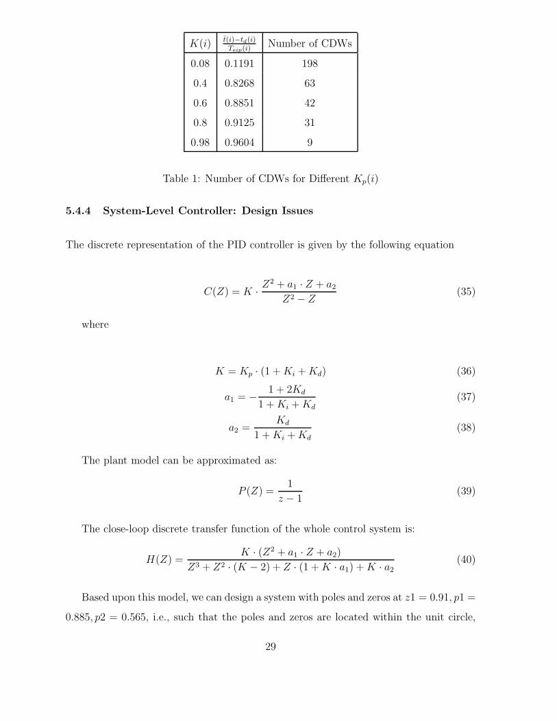
In Table 1 we show how the choice of Kp(i) affects the number of CDWs per one illumi-
nation period. We also show the value of the left hand side of Equation 34 to indicate
that the condition defined by this Equation is satisfied.
If we knew the distance to a given emitter, provided that we know the illumination
period of the emitter and the speed of the platform motion, we should be able to pick
an appropriate K(i), which guarantees detection while not overloading the receiver with
too many requests for dwells (number of CDWs). However, if this kind of knowledge is
not available, we need to select a more conservative approach. For an emitter with a long
illumination period we can choose a controller with a large K(i) resulting in fewer CDWs.
For a system with a shorter illumination period, we can choose a controller with a small
K(i), which can generate more CDWs but will give a higher probability of detection.
28
K(i) t(i)−td(i)Teip(i)
Number of CDWs
0.08 0.1191 198
0.4 0.8268 63
0.6 0.8851 42
0.8 0.9125 31
0.98 0.9604 9
Table 1: Number of CDWs for Different Kp(i)
5.4.4 System-Level Controller: Design Issues
The discrete representation of the PID controller is given by the following equation
C(Z) = K · Z2 + a1 · Z + a2
Z2 − Z(35)
where
K = Kp · (1 + Ki + Kd) (36)
a1 = − 1 + 2Kd
1 + Ki + Kd(37)
a2 =Kd
1 + Ki + Kd(38)
The plant model can be approximated as:
P (Z) =1
z − 1(39)
The close-loop discrete transfer function of the whole control system is:
H(Z) =K · (Z2 + a1 · Z + a2)
Z3 + Z2 · (K − 2) + Z · (1 + K · a1) + K · a2(40)
Based upon this model, we can design a system with poles and zeros at z1 = 0.91, p1 =
0.885, p2 = 0.565, i.e., such that the poles and zeros are located within the unit circle,
29

which results in a stable system. For instance, using Routh-Hurwitz method we can find
the values of the PID parameters Ki = 0.5, Ki = 0.1 and Kd = 0.0.
6 Simulation Results
We simulated a scenario in which a platform was moving along the straight line shown
in Figure 5. The speed of the platform was 1000 miles/hour. It took the platform 230
sec to travel the path.
Figure 5: Simulation Scenario
There were twenty four emitters in the scenario. The characteristics of the emitters
are shown in Table 2. We simulated both light and heavy load scenarios. Since for a
light load the performance of a dynamic scan scheduler is roughly the same as for a FSS,
we focused on heavy workloads.
The strength of the signal at the receiver was changing according to the following
equation:
30

Emitter fe Tpri Tpw Teip Be x, y
ID GHz sec sec sec degree [mile, mile]
1 2.25 2.0 · 10−3 4.5 · 10−5 10.0 4.0 [5.00, 10.0]
2 3.25 3.0 · 10−3 3.5 · 10−5 10.0 4.0 [7.00, 8.00]
3 5.25 4.0 · 10−3 2.5 · 10−5 10.0 4.0 [5.00, 40.0]
4 4.25 3.5 · 10−3 1.3 · 10−5 15.0 3.0 [7.00, 36.0]
5 6.25 2.5 · 10−3 2.6 · 10−5 15.0 3.0 [10.0, 30.0]
6 8.25 1.5 · 10−3 3.9 · 10−5 15.0 3.0 [13.0, 32.0]
7 7.75 2.5 · 10−3 2.0 · 10−5 18.0 3.5 [10.0, 15.0]
8 4.75 3.5 · 10−3 3.0 · 10−5 18.0 3.5 [12.0, 13.0]
9 5.75 4.5 · 10−3 4.0 · 10−5 18.0 3.5 [15.0, 25.0]
10 3.75 0.8 · 10−3 4.0 · 10−5 12.0 3.0 [13.0, 27.0]
11 2.75 1.6 · 10−3 3.0 · 10−5 12.0 3.0 [15.0, 20.0]
12 6.75 2.4 · 10−3 2.0 · 10−5 12.0 3.0 [14.0, 18.0]
13 11.25 2.0 · 10−4 4.5 · 10−6 5.0 2.0 [8.00, 12.0]
14 13.25 3.0 · 10−4 3.5 · 10−6 5.0 2.0 [13.0, 6.00]
15 15.25 4.0 · 10−4 2.5 · 10−6 5.0 2.0 [10.0, 39.0]
16 17.25 3.5 · 10−4 1.3 · 10−6 4.0 2.0 [6.00, 42.0]
17 16.25 2.5 · 10−4 2.6 · 10−6 4.0 2.0 [9.00, 27.0]
18 14.25 1.5 · 10−4 3.9 · 10−6 4.0 2.0 [8.00, 32.0]
19 12.25 2.5 · 10−4 2.0 · 10−6 6.00 2.5 [12.0, 12.0]
20 14.75 3.5 · 10−4 3.0 · 10−6 6.00 2.5 [14.0, 12.0]
21 16.75 4.5 · 10−4 4.0 · 10−6 6.00 2.5 [13.0, 25.0]
22 13.75 0.8 · 10−4 4.0 · 10−6 3.0 2.0 [12.0, 22.0]
23 15.75 1.6 · 10−4 3.0 · 10−6 3.0 2.0 [15.0, 22.0]
24 11.75 2.4 · 10−4 2.0 · 10−6 3.0 2.0 [13.0, 23.0]
Table 2: Characteristics of Simulated Emitters
31

Ar =Ae · e−(θ−φ)2/Be
2
r2(41)
where Ar and Ae are the signal strengths at the receiver and emitter, respectively, φ and
θ are the angle of the beam line of the emitter and the angle between the receiver and the
emitter, respectively, Be is the beam width, and r is the distance between the receiver
and the emitter. The illumination was detected if the strength Ar of the signal at the
emitter exceeded the noise threshold of the receiver.
In Figure 6 we show the distribution of the QoS for a FSS and for a DSS. The workload
for this scenario was 2.7967. From this figure, we can see that the values of the QoS for
the DSS are much lower than for the FSS. Since the QoS represents the uncertainty about
the state of an emitter, the lower the QoS the better.
Figure 6: Distribution of Mean QoS; Workload = 2.7967
In Figure 7 we show the distribution of the average maximal value of the QoS. From
this figure we can see that the system responds to the controllers very well. The maximal
value of the QoS does not cross the reference value of P (i), which in this experiment was
set to 1 for all emitters. The performance of the DSS is much better that of the FSS. The
32

FSS’s maximal QoS has a tendency to grow. The maximal QoS is an indication of the
stability of the system. Roughly, the system is stable if the value of the QoS is bounded.
Figure 7 shows that in the simulations the DSS showed a stable behavior.
Figure 7: Distribution of Max QoS
7 Conclusions and Future Research
In this paper we present a new approach to receiver scheduling based upon the control
theory metaphor of software development. We propose two metrics (the workload and the
quality of service) used to provide feedback on the quality of performance of the scheduler
and as controlled variables. These metrics are based on a simple and analytically tractable
model of quality of service that is integrated into scheduling logic. We also propose to
use a simple control logic for adjusting the parameters of a sensor scheduling policy
with very limited model complexity, making it appropriate for fast real-time scheduling
of sensors. We show that by an appropriate selection of the controller parameters the
system exhibits a stable performance and discuss how to select such parameters.
The experimental results illustrate the value of the approach. From the results of the
simulations it can be seen that the performance of the control based DSS is dramatically
33

better than that of the FSS in both accuracy and the number of CDW s especially when
the system is overloaded. The QoS for the control based DSS is much lower and, at the
same time, the number of CDW s is reduced to only one tenth of the CDW s in the FSS.
This is understandable since our DSS does not assume that the illumination period is
constant. Instead, it settles on a fixed period only through the application of its control
law. This gives it the robustness that is especially important when the environment
undergoes dynamic changes.
Although by using the control theory metaphor we achieved great improvement over
the fixed scan scheduler, we still have room for optimization of this solution. For instance,
we are implementing one more control loop to directly control the time spent for the
computation of schedules. This is a very important issue in our application since the
time scale of the scheduling is comparable to the time scale of computation. And thus
the issue of complexity of computation needs to be addressed. Furthermore, we need to
consider a more complex scenario in which there are multiple receivers as well as multiple
emitters. This leads naturally to a distributed control architecture.
Another problem that needs to be addressed is the development of rules for mapping
applications to the control theory based architectures. The mapping is currently being
performed in an ad hoc manner based on experience. A more systematic approach would
make it much easier for the control theory metaphor to be applied by the general software
community. We made some advances in this direction in [18].
Acknowledgments
This research was partially supported by the Defense Advanced Research Projects Agency
under contract F330602-99-C-0167. We are grateful to many people for helpful conversa-
tions and suggestions, most notably Kevin Passino, Mark MacBeth, Paul Zemany, Artan
Simeqi and Fengming Zhang. Moreover, the we would like to express our gratitude to
the anonymous reviewers whose constructive criticism helped us improve the clarity and
the readability of this paper.
34
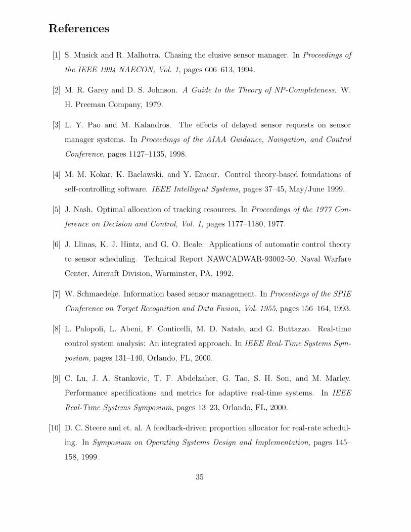
References
[1] S. Musick and R. Malhotra. Chasing the elusive sensor manager. In Proceedings of
the IEEE 1994 NAECON, Vol. 1, pages 606–613, 1994.
[2] M. R. Garey and D. S. Johnson. A Guide to the Theory of NP-Completeness. W.
H. Preeman Company, 1979.
[3] L. Y. Pao and M. Kalandros. The effects of delayed sensor requests on sensor
manager systems. In Proceedings of the AIAA Guidance, Navigation, and Control
Conference, pages 1127–1135, 1998.
[4] M. M. Kokar, K. Baclawski, and Y. Eracar. Control theory-based foundations of
self-controlling software. IEEE Intelligent Systems, pages 37–45, May/June 1999.
[5] J. Nash. Optimal allocation of tracking resources. In Proceedings of the 1977 Con-
ference on Decision and Control, Vol. 1, pages 1177–1180, 1977.
[6] J. Llinas, K. J. Hintz, and G. O. Beale. Applications of automatic control theory
to sensor scheduling. Technical Report NAWCADWAR-93002-50, Naval Warfare
Center, Aircraft Division, Warminster, PA, 1992.
[7] W. Schmaedeke. Information based sensor management. In Proceedings of the SPIE
Conference on Target Recognition and Data Fusion, Vol. 1955, pages 156–164, 1993.
[8] L. Palopoli, L. Abeni, F. Conticelli, M. D. Natale, and G. Buttazzo. Real-time
control system analysis: An integrated approach. In IEEE Real-Time Systems Sym-
posium, pages 131–140, Orlando, FL, 2000.
[9] C. Lu, J. A. Stankovic, T. F. Abdelzaher, G. Tao, S. H. Son, and M. Marley.
Performance specifications and metrics for adaptive real-time systems. In IEEE
Real-Time Systems Symposium, pages 13–23, Orlando, FL, 2000.
[10] D. C. Steere and et. al. A feedback-driven proportion allocator for real-rate schedul-
ing. In Symposium on Operating Systems Design and Implementation, pages 145–
158, 1999.
35

[11] C. Lu, J. A. Stankovic, G. Tao, and S. H. Son. Design and evaluation of a feedback
control EDF scheduling algorithm. In IEEE Real-Time Systems Symposium, pages
56–67, Phoenix, AZ, 1999.
[12] J. W. S. Liu. Real-Time Systems. Prentice Hall, 2000.
[13] M. Klein, T. Ralya, B. Pollak, R. Obenza, and M. G. Harbour. A Practitioner’s
Handbook for Real-Time Analysis: Guide to Rate Monotonic Analysis for Real-Time
Systems. Kluwer Academic Publishers, 1993.
[14] M. G. Harbour, M. H. Klien, and J. P. Lehoczky. Fixed priority scheduling of
periodic tasks with varying execution priorities. Proceedings of IEEE Real-Time
Systems Symposium, pages 116–128, 1991.
[15] J. P. Lehoczky, L. Sha, and Y. Ding. The rate monotonic scheduling algorithm
- exact characterization and average case behavior. In IEEE Real-Time Systems
Symposium, pages 166–171, 1989.
[16] P. Mejia-Alvarez, R. Melhem, and D. Mosse. An incremental approach to scheduling
during overloads in real-time systems. In IEEE Real-Time Systems Symposium,
pages 283–294, 2000.
[17] D. Seto, J. P. Lehoczky, L. Sha, and K. G. Shin. On task schedulability in real-time
control systems. In IEEE Real-Time Systems Symposium, pages 13–21, 1996.
[18] M. M. Kokar, K. M. Passino, K. Baclawski, and J. E. Smith. Mapping an application
to a control architecture: Specification of the problem. Lecture Notes in Computer
Science, 1936:75–89, 2001.
[19] K. J. Hintz. A measure of the information gain attributable to cueing. IEEE
Transactions on Systems, Man and Cybernetics, 21, No. 2:237–244, 1991.
[20] K. J. Hintz and E. S. McVey. Multi-process constrained estimation. IEEE Transac-
tions on Systems, Man and Cybernetics, 21, No. 1:434–442, 1991.
36

[21] D. A. Castanon. Approximate dynamic programming for sensor management. In
Proceedings, IEEE Conference on Decision and Control, pages 1202–1207, 1997.
[22] R. Rajkumar, C. Lee, J. Lehoczky, and D. Siewiorek. Practical solutions for QoS-
based resource allocation problems. In IEEE Real-Time Systems Symposium, pages
296–306, 1998.
[23] D. Hull, A. Shankar, K. Nahrstedt, and J. W. S. Liu. An end-to-end QoS model
and management architecture. In IEEE Real-Time Applications Symposium, pages
176–189, 1997.
[24] C. Aurrecoechea, A Cambell, and L. Hauw. A survey of QoS architectures. In 4th
IFIP International Conference on Quality of Service, pages 138–151, 2001.
[25] S. G. Bier and P. Rothman. Intelligent sensor management for beyond visual range
air-to-air combat. In Proceedings of the IEEE 1988 NAECON, pages 264–269, 1988.
[26] G. Buttazzo, G. Lipari, and G. Abeni. Elastic task model for adaptive rate control.
In IEEE Real-Time Systems Symposium, pages 286–295, 1998.
[27] D. Rosu, K. Schwan, and S. Yalamanchili. FARA - a framework for adaptive re-
source allocation in complex real-time systems. In IEEE Real-Time Technology and
Applications Symposium, pages 79–84, 1998.
[28] D. Rosu, K. Schwan, S. Yalamanchili, and R. Jha. On adaptive resource allocation
for complex real-time applications. In IEEE Real-Time Systems Symposium, pages
320–329, 1997.
37