contributions to the empirical analysis of addictive behaviors · contributions to the empirical...

Contributions to the empirical analysis of addictive behaviors

UVic, Feb 12, 2010Chris Auld

I will present a discussion of three papers which focus on empirical methods to studyaddictive behaviors, narrowly defined in the sense that I mean methods to measureaddiction itself rather than the broader literature on all aspects of addictive goods. Twoof these papers were published a few years ago, the other is a current working paper.The remainder of this document is copies of the papers.

Auld, M. C. and Grootendorst, P. (2004) An empirical analysis of milk addiction.Journal of Health Economics 23(6):1117-1133.

Abstract. We show the estimable rational addiction model tends to yield spurious evi-dence in favor of the rational addiction hypothesis when aggregate data are used. Directapplication of the canonical model yields results seemingly indicative that non-addictivecommodities such as milk, eggs, and oranges are rationally addictive. Monte Carlo simu-lation demonstrates that such results are likely to obtain whenever the commodity underscrutiny exhibits high serial correlation, or when even a small amount of the variation inprices is endogenous, or when overidentified instrumental variables estimators are used,or when commonly imposed restrictions are employed. We conclude that time-seriesdata will often be insufficient to differentiate rational addiction from serial correlationin the consumption series.

Auld, M. C. and Zarrabi, M. (2009) Long term effects of tobacco taxes faced byadolescents. Manuscript (submitted to Health Economics).

Abstract. We estimate the effects of tobacco prices faced in adolescence on smokingpatterns of adults aged 19 to 40. Use of large repeated cross-sectional surveys in Canadain the early 2000s allows us to exploit substantial and plausibly exogenous tax changesacross time and regions which occurred roughly a decade earlier. Results from a varietyof econometric techniques suggest that there is a small but detectable long run effectof price faced during adolescence. A 10% increase in prices faced during adolescence,holding contemporaneous prices constant, leads to at most a 1% reduction in smokingpropensity and intensity in early to mid adulthood, and we cannot reliably reject thehypothesis that the long term effect is zero. The results are sensitive to specificationand to how price during adolescence is measured.

Auld, M. C. (2005) Causal effect of early initiation on adolescent smoking patterns.Canadian Journal of Economics 38(3):709-34.

Abstract. A key concern in policy debates over youth smoking is whether preventingchildren from smoking will stop them from smoking as adults or merely defer initiationinto smoking. This paper estimates determinants of smoking status in late adolescenceviewing smoking at age 14 as an endogenous treatment on subsequent smoking. Thisapproach disentangles causation from unobserved heterogeneity and allows addictivenessto vary across individuals. Exploiting large tax changes across time and across regions inCanada in the early 1990s, the estimated model suggests that smoking is highly addictivefor the average youth but less so for youths who actually do initiate early or who arelikely to be induced to initiate early at the margin. Thus, policies that deter initiationwill reduce eventual smoking rates, but not by as large a magnitude as conventionaleconometric models might suggest.

Journal of Health Economics 23 (2004) 1117–1133

An empirical analysis of milk addiction

M. Christopher Aulda,∗, Paul Grootendorstb

a Department of Economics, Faculty of Social Sciences, University of Calgary,Calgary, Alta., Canada T2N 1N4

b Faculty of Pharmacy, University of Toronto, Toronto, Canada

Received 2 October 2003; accepted 26 February 2004Available online 9 June 2004

Abstract

We show the estimable rational addiction model tends to yield spurious evidence in favor ofthe rational addiction hypothesis when aggregate data are used. Direct application of the canonicalmodel yields results seemingly indicative that non-addictive commodities such as milk, eggs, andoranges are rationally addictive. Monte Carlo simulation demonstrates that such results are likelyto obtain whenever the commodity under scrutiny exhibits high serial correlation, or when even asmall amount of the variation in prices is endogenous, or when overidentified instrumental variablesestimators are used, or when commonly imposed restrictions are employed. We conclude thattime-series data will often be insufficient to differentiate rational addiction from serial correlationin the consumption series.© 2004 Elsevier B.V. All rights reserved.

JEL classification: C15; C32; I12

Keywords: Rational addiction; Monte Carlo simulation; Instrumental variables

1. Introduction

A large literature has arisen followingBecker and Murphy’s (1988)theory of ratio-nal addiction. The model has been implemented empirically to study numerous activi-ties, including use of drugs such as tobacco, alcohol, cocaine, opium, and caffeine, andactivities such as gambling, cinema, and eating.1 Frequently, evidence for rational addic-

∗ Corresponding author. Tel.:+1-403-220-4098; fax:+1-403-282-5262.E-mail address: [email protected] (M.C. Auld).

1 Respectively, see:Becker et al. (1994), Baltagi and Griffin (2002), Grossman and Chaloupka (1998), Liu et al.(1999), Olekalns and Bardsley (1996), Mobilia (1993), Cameron (1999), andCawley (1999).

0167-6296/$ – see front matter © 2004 Elsevier B.V. All rights reserved.doi:10.1016/j.jhealeco.2004.02.003

1118 M.C. Auld, P. Grootendorst / Journal of Health Economics 23 (2004) 1117–1133

tion is found, although the results are often described as less than compelling since unstabledemand, implausible discount rates, and low price elasticities are estimated (Cameron, 1998;Ferguson, 2000; Baltagi and Griffin, 2001). Further,Gruber and Koszegi (2001)show thatreduced form estimates ofBecker et al. (1994)seminal model of cigarette demand is frag-ile to whether it is estimated in levels or differences. We contribute to the discussion byinvestigating the small-sample properties of commonly employed models. First, we pro-pose an ‘anti-test’ of the empirical rational addiction model: We show that its applicationto time-series data on consumption of milk, eggs, oranges, apples, and cigarettes yields“evidence” that milk—by a substantial margin—is the most rationally addictive of thesecommodities. We then explain this result, and many of the anomalous results in the litera-ture, through Monte Carlo simulation of demand models in which rational addiction is notpresent by construction. We show that the standard methodology is generally biased in thedirection of finding rational addiction. Spurious evidence for rational addiction is likely toobtain if: (1) the consumption series is highly autocorrelated, (2) even a small amount ofthe variation in prices is endogenous, (3) a common linear restriction—that the ratio of thecoefficient on the lead of consumption to that on the lag is the discount rate—is imposedon the model, or (4) overidentified instrumental variable estimators are used.

The rational addiction hypothesis holds that individuals have stable preferences andcorrectly anticipate that increases in current consumption of an addictive good will playout in the future as increased marginal utility of consumption. From that simple premise,the model is able to mimic many observed features of addiction, including “cold turkey”quitting behavior, reinforcement, tolerance, and withdrawal. We take no issue with thetheory per se, but rather with the interpretation of some of the empirical evidence relatingto the hypothesis.Becker et al. (1994)present the canonical empirical version of the modelin the context of a careful analysis of US cigarette consumption. Current consumption of apotentially addictive good is regressed on its first lag and lead, current price, and possiblyother demand shifters. The lags and leads of consumption are instrumented with lags andleads of prices. Positive estimates of the coefficients on the lag and the lead are interpretedas evidence for the rational addiction hypothesis, and the ratio of the coefficient on the leadto that on the lag is interpreted as an estimate of the discount rate.

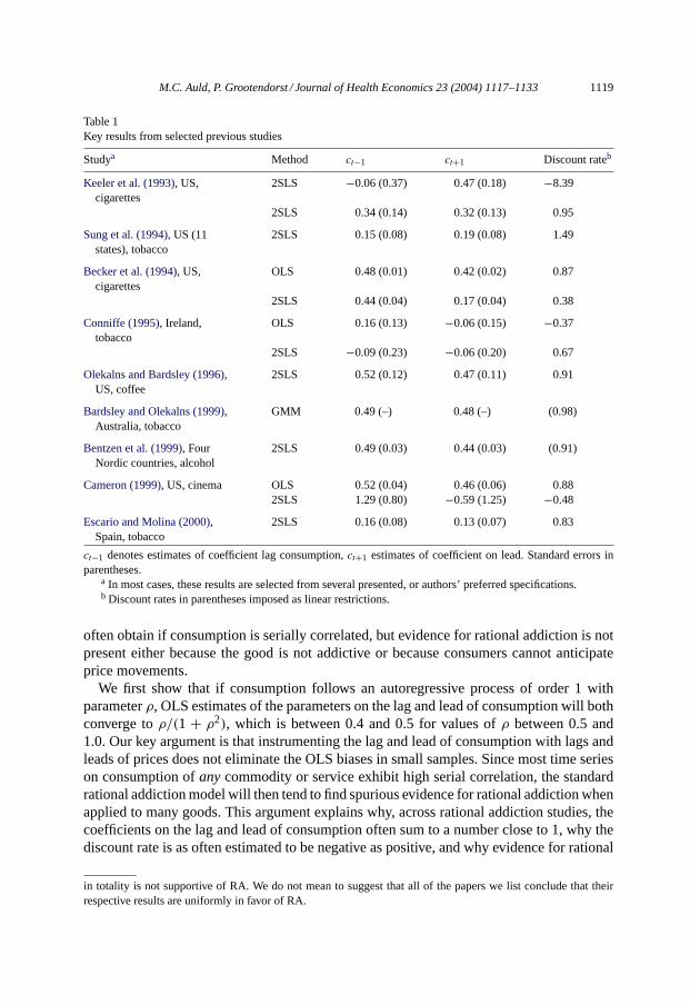
An extensive meta-analysis of the empirical literature on rational addiction is beyondthe scope of this paper, however, inTable 1we present some selected results from selectedstudies using aggregate data to estimate such models for several different goods. Wherepossible, ordinary least squares (OLS) and instrumental variables estimates are compared.Several stylized facts stand out. First, estimates of the discount rate are highly variable,frequently negative, subject to occasional extreme draws, and estimates can be sensitive towhether it is imposed or left free to vary. Second, instrumental variables estimates are muchmore variable than OLS estimates. Third, the coefficients on the lag and lead of consumptionare usually positive and often sum to close to unity, particularly when OLS is employed.Fourth, in all but two of the specifications presented the coefficient on lead consumption ispositive and statistically significant. Such results are typically but not always interpreted asevidence in favor of rational addiction.2 We present evidence that all of these results will

2 Indeed, some authors are skeptical that their results genuinely reflect RA. For example, we have reportedKeeler et al.’s (1993)estimates constrained to be consistent with RA, but the authors argue that their evidence

M.C. Auld, P. Grootendorst / Journal of Health Economics 23 (2004) 1117–1133 1119

Table 1Key results from selected previous studies

Studya Method ct−1 ct+1 Discount rateb

Keeler et al. (1993), US,cigarettes

2SLS −0.06 (0.37) 0.47 (0.18) −8.39

2SLS 0.34 (0.14) 0.32 (0.13) 0.95

Sung et al. (1994), US (11states), tobacco

2SLS 0.15 (0.08) 0.19 (0.08) 1.49

Becker et al. (1994), US,cigarettes

OLS 0.48 (0.01) 0.42 (0.02) 0.87

2SLS 0.44 (0.04) 0.17 (0.04) 0.38

Conniffe (1995), Ireland,tobacco

OLS 0.16 (0.13) −0.06 (0.15) −0.37

2SLS −0.09 (0.23) −0.06 (0.20) 0.67

Olekalns and Bardsley (1996),US, coffee

2SLS 0.52 (0.12) 0.47 (0.11) 0.91

Bardsley and Olekalns (1999),Australia, tobacco

GMM 0.49 (–) 0.48 (–) (0.98)

Bentzen et al. (1999), FourNordic countries, alcohol

2SLS 0.49 (0.03) 0.44 (0.03) (0.91)

Cameron (1999), US, cinema OLS 0.52 (0.04) 0.46 (0.06) 0.882SLS 1.29 (0.80) −0.59 (1.25) −0.48

Escario and Molina (2000),Spain, tobacco

2SLS 0.16 (0.08) 0.13 (0.07) 0.83

ct−1 denotes estimates of coefficient lag consumption,ct+1 estimates of coefficient on lead. Standard errors inparentheses.

a In most cases, these results are selected from several presented, or authors’ preferred specifications.b Discount rates in parentheses imposed as linear restrictions.

often obtain if consumption is serially correlated, but evidence for rational addiction is notpresent either because the good is not addictive or because consumers cannot anticipateprice movements.

We first show that if consumption follows an autoregressive process of order 1 withparameterρ, OLS estimates of the parameters on the lag and lead of consumption will bothconverge toρ/(1 + ρ2), which is between 0.4 and 0.5 for values ofρ between 0.5 and1.0. Our key argument is that instrumenting the lag and lead of consumption with lags andleads of prices does not eliminate the OLS biases in small samples. Since most time serieson consumption ofany commodity or service exhibit high serial correlation, the standardrational addiction model will then tend to find spurious evidence for rational addiction whenapplied to many goods. This argument explains why, across rational addiction studies, thecoefficients on the lag and lead of consumption often sum to a number close to 1, why thediscount rate is as often estimated to be negative as positive, and why evidence for rational

in totality is not supportive of RA. We do not mean to suggest that all of the papers we list conclude that theirrespective results are uniformly in favor of RA.


addiction is found even when it is implausible that consumers have information on futureprice changes.

The paper is organized as follows.Section 2presents estimates of the canonical estimablerational addiction model applied to Canadian time-series data on cigarettes and four pre-sumably non-addictive goods. We find that milk appears to be more rationally addictivethan cigarettes, a result we dismiss out of hand and explain via analysis and simulationspresented inSection 3. Section 4concludes the paper.

2. Rational addiction to milk

In order to be a useful empirical tool, the estimable rational addiction (RA) model must beable to discriminate between addictive and non-addictive goods. In this section we proposean ‘anti-test’ of the RA model’s ability to differentiate addictive and non-addictive goodssimilar in the spirit ofDranove and Wehner’s (1994)tests for supplier-induced demand. Weestimate RA models for both cigarettes, which we assume actually are addictive, and forseveral common staples which should not be found to be addictive.

FollowingBecker, Grossman, and Murphy et al. (1994)(BGM), the canonical empiricalimplementation of the rational addiction model can be sketched as follows. Consumersmaximize lifetime utility

∞∑t=0

βtU(ct, ct−1, yt, et) (1)

subject to a law of motion for assets, wherect is the consumption of a possibly addictivegood in periodt, yt consumption of a numeraire,et represents the influence of variablesobserved by the agent but not the econometrician, andβ the agent’s discount rate. If theperiod return is quadratic, the optimal path for consumption follows a difference equationof the form

ct = θct−1 + βθct+1 + θ1pt + ut, (2)

where theθ’s are parameters which depend on the underlying preferences andut is thenoise. This equation is typically estimated via instrumental variables techniques since theorypredicts that both the lag and lead of consumption are endogenous because a shock toetwill affect marginal utility in all periods. BGM used, variously, lags and leads of prices andtax rates of various orders as instruments. In their preferred specification, the estimate ofθ

is 0.418 and the coefficient onct+1 is 0.138. BGM interpret the former result as verifyingthe addictive nature of the good, and the latter as evidence against myopic behavior, that is,as evidence in favor ofrational addiction.

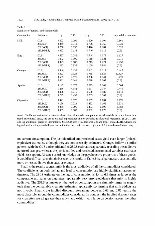
In Table 3, we present estimates ofEq. (2)applied to annual aggregate Canadian dataon cigarettes, and on a number of goods we selected on the basis that rational addictivebehavior can be ruled out a priori: milk, eggs, oranges, and apples. Summary statistics anddetails of the data are presented inTable 2. In each case, we include a linear time trend anda measure of real per-capita outlays on consumer non-durables as a proxy for permanentincome. For each commodity, we consider four estimators: OLS, just identified two-stage


Table 2Summary statistics

Variable Units CANSIM Period n Mean S.D.

Milk quantity Liters D267578 1961–2000 40 94.82 5.32Milk price P100021 1961–2000 40 1.02 0.08

Egg quantity Dozens D267584 1961–2000 40 18.04 2.62Egg price P100026 1961–2000 40 1.42 0.33

Orange quantity kg D265449 1960–2000 41 9.71 1.30Orange price P100040 1960–2000 41 1.19 0.17

Apple quantity kg D264858 1960–2000 41 11.57 1.26Apple price P100039 1960–2000 41 0.82 0.13

Cigarette quantity Cigarettes D2091, D2095 1968–2000 33 2161.61 427.73Cigarette price P200267 1968–2000 33 0.54 0.19

Outlays D16141, D16142 1961–2000 40 10895.89 2344.28

Notes: All data are annual and national-level and were obtained from the Statistics Canada’s CANSIM database.“Outlays” is per-capita spending on consumer non-durable goods and services. Outlays and all prices expressed inreal terms by adjusting by all-items CPI(1992= 100). All quantities in per-capita terms. Cigarette consumptionincludes cigars and is the sum of domestic and export sales, as the vast majority of exports are smuggled back intoCanada (Galbraith and Kaiserman, 1997).

least squares (2SLS) using one lag and lead of prices as instruments for the lags and leadsof consumption (2SLS(JI)), an overidentified 2SLS estimator using three lags and threeleads of prices as instruments (2SLS(OI)), and finally 2SLS estimates imposing the linearrestriction that the coefficient onct+1 equals the discount rate times the coefficient onct−1,again using one lag and lead of price as instruments (2SLS(RES)). We set the discount ratein the last case at 0.9.

The cigarette models confirm the result that cigarettes are rationally addictive. Each of theestimators yields positive coefficients on the lag and lead of consumption, suggesting higherpast or future consumption causes higher current consumption, although the coefficient onthe lag of consumption in the 2SLS(JI) case is not statistically significant. The implieddiscount rates are, however, implausible, ranging from about 1.2 to almost 4.0. BGM andother authors have found similar results and interpreted them, in the phrasing ofBaltagi andGriffin (2001), as “verifying addiction” and “clearly rejecting myopic addiction” despitethe “disquieting anomalies” that appear.

Among the presumably non-addictive commodities, apples provide the least support forRA, as the coefficients on lag and lead consumption are statistically insignificant acrossestimators. However, even in this case one could argue there is weak support for RA. Thecoefficients are always positive, and seem to settle down to values similar to those we recoverfor cigarettes as more instruments or the restriction are used, although the elasticities areimprecisely estimated. Anticipating results discussed in the following section, we note herethat apple consumption exhibits the least serial correlation of our five commodities.

There is evidence for the rational addictiveness of eggs and oranges comparable, albeitsomewhat weaker, to that for cigarettes. In the case of eggs, the OLS and overidentified2SLS estimates indicate large and precisely estimated effects of past and future consumption


Table 3Estimates of rational addiction models

Commodity Estimator ct−1 S.E. ct+1 S.E. Implied discount rate

Milk OLS 0.603 0.099 0.520 0.104 0.8612SLS(JI) 0.849 0.312 0.706 0.365 0.8302SLS(OI) 0.756 0.195 0.476 0.181 0.6282SLS(RES) 0.822 0.132 0.740 0.119 (0.9)

Eggs OLS 0.497 0.086 0.548 0.073 1.1272SLS(JI) 1.472 3.109 1.118 1.021 0.7752SLS(OI) 0.327 0.188 0.713 0.224 2.2302SLS(RES) 1.232 0.938 1.109 0.844 (0.9)

Oranges OLS 0.546 0.133 0.242 0.117 0.4472SLS(JI) 0.023 0.524 −0.735 0.636 −32.8272SLS(OI) 0.555 0.170 0.268 0.144 0.4782SLS(RES) 0.031 0.341 0.028 0.307 (0.9)

Apples OLS 0.147 0.175 0.075 0.202 0.5042SLS(JI) 1.256 4.682 0.567 2.347 0.4462SLS(OI) 0.496 1.010 0.550 1.189 1.1182SLS(RES) 0.295 1.452 0.265 1.307 (0.9)

Cigarettes OLS 0.441 0.078 0.507 0.081 1.1762SLS(JI) 0.128 0.224 0.492 0.162 3.9312SLS(OI) 0.365 0.099 0.493 0.095 1.3882SLS(RES) 0.369 0.087 0.332 0.078 (0.9)

Notes: Coefficient estimates reported as elasticities calculated at sample means. All models include a linear timetrend, current real price, and per-capita real expenditures on non-durables as additional regressors. 2SLS(JI) usesone lag and lead of prices as instruments, 2SLS(OI) uses two additional lags and leads, and 2SLS(RES) uses onelag and lead and imposes the linear restriction that the coefficient onct+1 equals 0.9 times the coefficient onct−1.

on current consumption. The just identified and restricted cases yield even larger (indeed,explosive) estimates, although they are not precisely estimated. Oranges follow a similarpattern, with the OLS and overidentified 2SLS estimators apparently revealing the addictivenature of oranges, whereas the just identified and restricted instrumental variables estimatesyield less support. Absent a priori knowledge on the psychoactive properties of these goods,it would be difficult to maintain based on the results inTable 3that cigarettes are substantiallymore or less addictive than eggs or oranges.

Finally, the results suggest milk is the most addictive of all the commodities considered.The coefficients on both the lag and lead of consumption are highly significant across es-timators. The 2SLS estimate on the lag of consumption is 1.4 to 6.6 times as large as thecomparable estimates on cigarettes, apparently very strong evidence that milk is highlyaddictive. The 2SLS estimates on the lead of consumption are similarly larger in magni-tude than the comparable cigarette estimates, apparently confirming that milk addicts arenot myopic. Finally, the implied discount rates range between 0.63 and 0.86, easily themost plausible among the commodities considered. In contrast, the implied discount ratesfor cigarettes are all greater than unity, and exhibit very large dispersion across the othercommodities.


In short, among the commodities considered, we find apples to be least rationally addic-tive. Eggs, cigarettes, and oranges are apparently comparably addictive, with mixed supportin favor of the RA hypothesis. Milk, however, is very strongly addictive! This is clearly anempirical puzzle since we can rule out the addictiveness of milk over tobacco on the basisof other evidence.

3. Analysis

We first examine the properties of OLS estimates ofEq. (2)when the errors are seriallycorrelated. Ignoring other covariates for the moment, suppose consumption follows anAR(1) process which we express as

ct = ut, ut = ρut−1 + εt, (3)

whereε is the mean-zero white noise with varianceσ2ε and the absolute value ofρ is not

greater than unity. Consider the regression ofct onto its lag and lead

ct = βlct−1 + βf ct+1 + ut. (4)

Notice that by construction there is neither rational addiction nor habit formation present(the true values ofβl andβf are zero). It is well known that the lag of consumption isendogenous when the errors are serially correlated, and the same is true of the lead ofconsumption: the covariance betweenct+1 andut is ρσ2

ε . The true values ofβl andβf arezero, but it can be shown that

plimn→∞

βl = plimn→∞

βf = ρ

1 + ρ2, (5)

whereβi, i = l, f represent the OLS estimates of (4) (seeAppendix A.1for proof). Further,notice that after holding the lag of consumption constant, the errors are serially uncorrelated.Thus, testing for and failing to find autocorrelation after estimating an equation such as (4)does not indicate that serial correlation is not biasing the results. When other covariatesXt are present the same arguments apply; the estimated coefficients on the columns ofXtwill generally not be consistently estimated and the coefficients on the lag and lead ofconsumption will converge to values which depend on bothρ and the covariances betweenthe columns ofXt and the consumption series.

Recall the implied discount rate is the ratio of the coefficient on the lead of consumptionto that on the lag of consumption. Since these coefficients are centered on the same value,OLS estimates of the RA equation will yield estimates of the discount rate centered onroughly unity. However, no moments of this ratio will generally exist even when the meanof the estimator exists (Hinckley, 1969) such that the estimated discount rate will exhibithigh variability and occasional very extreme draws.

We are also now in a position to explainGruber and Koszegi’s (2001)finding that estima-tion of BGMs cigarette demand equations are sensitive to estimation in differences versuslevels. Suppose thatEq. (4)is estimated in differences when the DGP is, as before, givenby Eq. (3). It is possible to show that

plimn→∞

βdl = plim

n→∞βd

f = ρ − 1

ρ2 − ρ + 2, (6)


where superscript d’s denote estimates of the differenced model (seeAppendix A.2forproof). The asymptotic bias is then well approximated by 0.5(−1+ρ) for ρ > 0, where theapproximation is exact atρ = 0 orρ = 1. If consumption has a unit root, the differencedmodel is consistent. The bias is approximately linear inρ, of the opposite sign, smaller inmagnitude forρ > 0.4 than in the levels case, and small for values ofρ typical of mosteconomic time series. For instance, atρ = 0.9, approximately the serial correlation in thecigarette data discussed inSection 2, the asymptotic bias in the differenced model would beapproximately−0.05, whereas in levels it is 0.497. We graph the asymptotic bias for levelsand differences models inFig. 1.

OLS estimates of the RA equation in levels then tend to yield spurious evidence infavor of RA whenever serial correlation is present in the consumption series, along withestimates of the discount rate centered on roughly unity. The endogeneity of both the lag andlead of consumption is well known, following from either serial correlation in the errorsor from optimizing behavior under rational addiction. Instrumental variables techniquesare, then, typically used to estimate (2). It is immediate from the argument above thatanything which biases instrumental variables estimates in the same direction as the OLSbias will yield misleading evidence in favor of the RA hypothesis whenever the consumptionseries exhibits significant serial correlation. If, however, prices are exogenous, instrumental

0 0.1 0.2 0.3 0.4 0.5 0.6 0.7 0.8 0.9 1-0.5

-0.4

-0.3

-0.2

-0.1

0

0.1

0.2

0.3

0.4

0.5

ρ

Bia

s

Levels

Differences

Fig. 1. Asymptotic bias of OLS models. Bias of lead consumption parameter estimate when consumption followsan AR(1) process with parameterρ.


variable estimates of the coefficients on the lag and lead of consumption are consistent. Wenow examine the small-sample properties of these estimators.

4. Monte Carlo simulations

4.1. Experimental design

We consider the data generating process (DGP)

ct = −ηpt + ut, ut = ρut−1 + εt, pt = 0.9pt−1 + νt,εt ∼ NID(0,1), νt ∼ NID(0,1), (7)

and the properties of the regression

ct = βlct−1 + βf ct+1 + βppt + noise. (8)

We are as generous to the rational addiction model as possible while still allowing theprice and consumption series to exhibit serial correlation. We assume prices are strictlyexogenous, we remove other covariates which is equivalent to assuming that we have alreadyperfectly captured and removed all other influences on consumption, and we assume awaymeasurement error (such as due to smuggling or hoarding), consumer uncertainty overfuture prices, and the other problems that previous research has identified in this context.Notice that the population values ofβl andβf are both zero, so there is by construction norational addiction present under DGP (7).

The estimators we consider are OLS(βOLSf ) and several variants of 2SLS: the just identi-

fied case using one lag and lead of prices as instruments(β2SLS(JI)f ), the overidentified case

using two lags and leads of consumption as instruments(β2SLS(OI)f ), and subject to the re-

strictionβf = 0.9βl , again using one lag and one lead of prices as instruments(β2SLS(RES)f ).

Since, as discussed above, the lag and lead of consumption are endogenous whenρ = 0,OLS is inconsistent. Since prices are valid instruments, each of the 2SLS estimators is con-sistent with variance proportional to the second diagonal element of (X′W(W′W)−1W′X)−1,whereX denotes the matrix of regressors in (8) andW the matrix of instruments. The exactsmall-sample properties of the estimates are very difficult to obtain even in considerablysimpler models (in related contexts, seePhillips, 1977; Bekker, 1994), so we simulate theirproperties.

We limit interest to the properties of estimators ofβf , the parameter usually interpretedas reflecting rational addiction, although we note that our findings will usually also apply tothe coefficient on the lag of consumption, which is conventionally interpreted as verifyingaddiction. We characterize the distribution ofβf and the size of thet-test against the (true)null that this parameter is zero using response surfaces. The parameters we are interestedin varying across experiments are the sample sizen, η, which governs the strength of theinstruments andρ, which governs the degree of autocorrelation the consumption seriesexhibits. We stratify by sample size since we expect sample size to interact with the otherparameters in a complex manner.


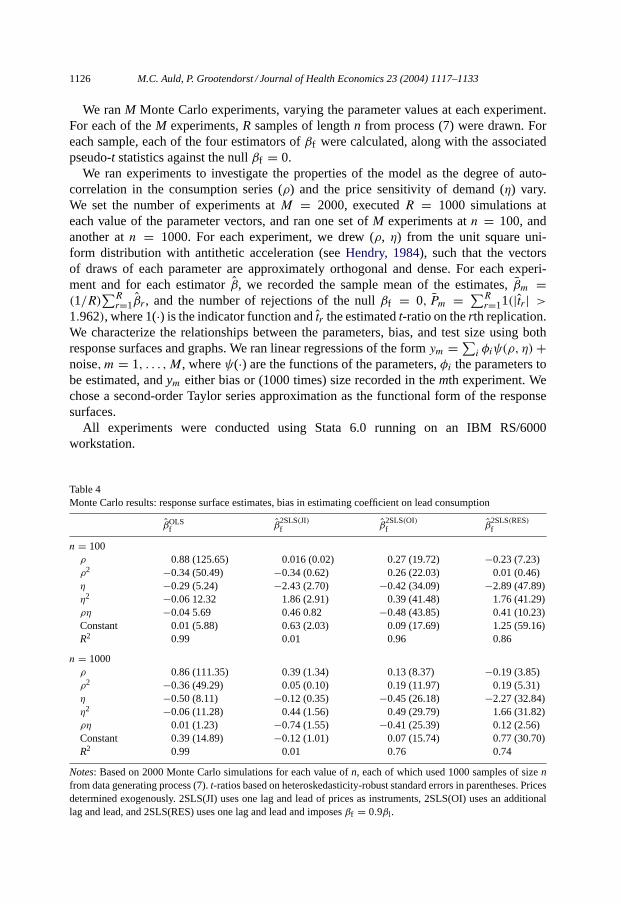
We ranM Monte Carlo experiments, varying the parameter values at each experiment.For each of theM experiments,R samples of lengthn from process (7) were drawn. Foreach sample, each of the four estimators ofβf were calculated, along with the associatedpseudo-t statistics against the nullβf = 0.

We ran experiments to investigate the properties of the model as the degree of auto-correlation in the consumption series (ρ) and the price sensitivity of demand (η) vary.We set the number of experiments atM = 2000, executedR = 1000 simulations ateach value of the parameter vectors, and ran one set ofM experiments atn = 100, andanother atn = 1000. For each experiment, we drew (ρ, η) from the unit square uni-form distribution with antithetic acceleration (seeHendry, 1984), such that the vectorsof draws of each parameter are approximately orthogonal and dense. For each experi-ment and for each estimatorβ, we recorded the sample mean of the estimates,βm =(1/R)

∑Rr=1βr, and the number of rejections of the nullβf = 0, Pm = ∑R

r=11(|tr| >1.962), where 1(·) is the indicator function andtr the estimatedt-ratio on therth replication.We characterize the relationships between the parameters, bias, and test size using bothresponse surfaces and graphs. We ran linear regressions of the formym = ∑

i φiψ(ρ, η)+noise,m = 1, . . . ,M, whereψ(·) are the functions of the parameters,φi the parameters tobe estimated, andym either bias or (1000 times) size recorded in themth experiment. Wechose a second-order Taylor series approximation as the functional form of the responsesurfaces.

All experiments were conducted using Stata 6.0 running on an IBM RS/6000workstation.

Table 4Monte Carlo results: response surface estimates, bias in estimating coefficient on lead consumption

βOLSf β

2SLS(JI)f β

2SLS(OI)f β

2SLS(RES)f

n = 100ρ 0.88 (125.65) 0.016 (0.02) 0.27 (19.72) −0.23 (7.23)ρ2 −0.34 (50.49) −0.34 (0.62) 0.26 (22.03) 0.01 (0.46)η −0.29 (5.24) −2.43 (2.70) −0.42 (34.09) −2.89 (47.89)η2 −0.06 12.32 1.86 (2.91) 0.39 (41.48) 1.76 (41.29)ρη −0.04 5.69 0.46 0.82 −0.48 (43.85) 0.41 (10.23)Constant 0.01 (5.88) 0.63 (2.03) 0.09 (17.69) 1.25 (59.16)R2 0.99 0.01 0.96 0.86

n = 1000ρ 0.86 (111.35) 0.39 (1.34) 0.13 (8.37) −0.19 (3.85)ρ2 −0.36 (49.29) 0.05 (0.10) 0.19 (11.97) 0.19 (5.31)η −0.50 (8.11) −0.12 (0.35) −0.45 (26.18) −2.27 (32.84)η2 −0.06 (11.28) 0.44 (1.56) 0.49 (29.79) 1.66 (31.82)ρη 0.01 (1.23) −0.74 (1.55) −0.41 (25.39) 0.12 (2.56)Constant 0.39 (14.89) −0.12 (1.01) 0.07 (15.74) 0.77 (30.70)R2 0.99 0.01 0.76 0.74

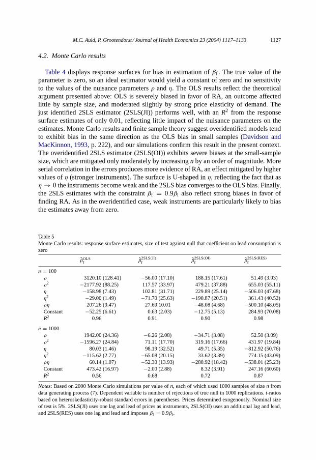
Notes: Based on 2000 Monte Carlo simulations for each value ofn, each of which used 1000 samples of sizenfrom data generating process (7).t-ratios based on heteroskedasticity-robust standard errors in parentheses. Pricesdetermined exogenously. 2SLS(JI) uses one lag and lead of prices as instruments, 2SLS(OI) uses an additionallag and lead, and 2SLS(RES) uses one lag and lead and imposesβf = 0.9βl .


4.2. Monte Carlo results

Table 4displays response surfaces for bias in estimation ofβf . The true value of theparameter is zero, so an ideal estimator would yield a constant of zero and no sensitivityto the values of the nuisance parametersρ andη. The OLS results reflect the theoreticalargument presented above: OLS is severely biased in favor of RA, an outcome affectedlittle by sample size, and moderated slightly by strong price elasticity of demand. Thejust identified 2SLS estimator (2SLS(JI)) performs well, with anR2 from the responsesurface estimates of only 0.01, reflecting little impact of the nuisance parameters on theestimates. Monte Carlo results and finite sample theory suggest overidentified models tendto exhibit bias in the same direction as the OLS bias in small samples (Davidson andMacKinnon, 1993, p. 222), and our simulations confirm this result in the present context.The overidentified 2SLS estimator (2SLS(OI)) exhibits severe biases at the small-samplesize, which are mitigated only moderately by increasingn by an order of magnitude. Moreserial correlation in the errors produces more evidence of RA, an effect mitigated by highervalues ofη (stronger instruments). The surface is U-shaped inη, reflecting the fact that asη→ 0 the instruments become weak and the 2SLS bias converges to the OLS bias. Finally,the 2SLS estimates with the constraintβf = 0.9βl also reflect strong biases in favor offinding RA. As in the overidentified case, weak instruments are particularly likely to biasthe estimates away from zero.

Table 5Monte Carlo results: response surface estimates, size of test against null that coefficient on lead consumption iszero

βOLSf β

2SLS(JI)f β

2SLS(OI)f β

2SLS(RES)f

n = 100ρ 3120.10 (128.41) −56.00 (17.10) 188.15 (17.61) 51.49 (3.93)ρ2 −2177.92 (88.25) 117.57 (33.97) 479.21 (37.88) 655.03 (55.11)η −158.98 (7.43) 102.81 (31.71) 229.89 (25.14) −506.03 (47.68)η2 −29.00 (1.49) −71.70 (25.63) −190.87 (20.51) 361.43 (40.52)ρη 207.26 (9.47) 27.69 10.01 −48.08 (4.68) −500.10 (48.05)Constant −52.25 (6.61) 0.63 (2.03) −12.75 (5.13) 284.93 (70.08)R2 0.96 0.91 0.90 0.98

n = 1000ρ 1942.00 (24.36) −6.26 (2.08) −34.71 (3.08) 52.50 (3.09)ρ2 −1596.27 (24.84) 71.11 (17.70) 319.16 (17.66) 431.97 (19.84)η 80.03 (1.46) 98.19 (32.52) 49.71 (5.35) −812.92 (50.76)η2 −115.62 (2.77) −65.08 (20.15) 33.62 (3.39) 774.15 (43.09)ρη 60.14 (1.07) −52.30 (13.93) −280.92 (18.42) −538.01 (25.23)Constant 473.42 (16.97) −2.00 (2.88) 8.32 (3.91) 247.16 (60.60)R2 0.56 0.68 0.72 0.87

Notes: Based on 2000 Monte Carlo simulations per value ofn, each of which used 1000 samples of sizen fromdata generating process (7). Dependent variable is number of rejections of true null in 1000 replications.t-ratiosbased on heteroskedasticity-robust standard errors in parentheses. Prices determined exogenously. Nominal sizeof test is 5%. 2SLS(JI) uses one lag and lead of prices as instruments, 2SLS(OI) uses an additional lag and lead,and 2SLS(RES) uses one lag and lead and imposesβf = 0.9βl .


Table 5presents response surface estimates for size of thet-test against the nullβf = 0.Again the OLS estimates display the worst properties, severely over-rejecting the null athigh values ofρ. The overidentified and restricted instrumental variables estimators farebetter than OLS, but still tend to over-reject the null when significant autocorrelation inconsumption is present.

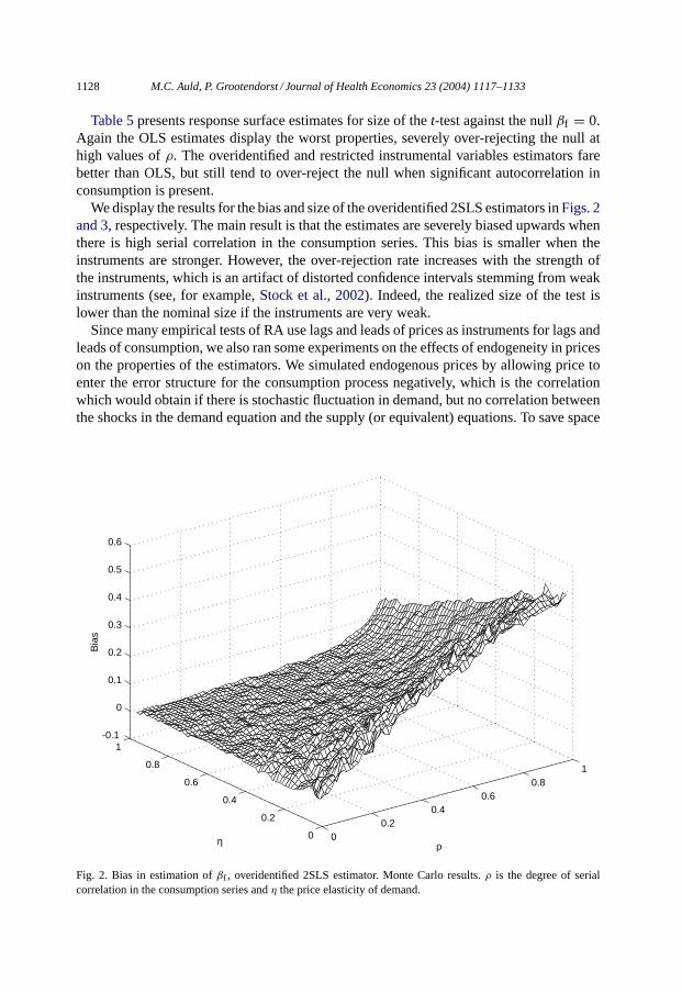
We display the results for the bias and size of the overidentified 2SLS estimators inFigs. 2and 3, respectively. The main result is that the estimates are severely biased upwards whenthere is high serial correlation in the consumption series. This bias is smaller when theinstruments are stronger. However, the over-rejection rate increases with the strength ofthe instruments, which is an artifact of distorted confidence intervals stemming from weakinstruments (see, for example,Stock et al., 2002). Indeed, the realized size of the test islower than the nominal size if the instruments are very weak.

Since many empirical tests of RA use lags and leads of prices as instruments for lags andleads of consumption, we also ran some experiments on the effects of endogeneity in priceson the properties of the estimators. We simulated endogenous prices by allowing price toenter the error structure for the consumption process negatively, which is the correlationwhich would obtain if there is stochastic fluctuation in demand, but no correlation betweenthe shocks in the demand equation and the supply (or equivalent) equations. To save space

00.2

0.40.6

0.81

0

0.2

0.4

0.6

0.8

1-0.1

0

0.1

0.2

0.3

0.4

0.5

0.6

ρη

Bia

s

Fig. 2. Bias in estimation ofβf , overidentified 2SLS estimator. Monte Carlo results.ρ is the degree of serialcorrelation in the consumption series andη the price elasticity of demand.


00.2

0.40.6

0.81

0

0.2

0.4

0.6

0.8

1-100

0

100

200

300

400

500

ρη

Siz

e (r

ejec

tions

per

1,0

00 d

raw

s)

Fig. 3. Size of test againstβf = 0, overidentified 2SLS estimator. Monte Carlo results.ρ is the degree of serialcorrelation in the consumption series,η the price elasticity of demand. Figure shows number of rejections per1000 draws of the true null that rational addiction is not present. Nominal size is 5%.

we do not report these results as, unsurprisingly, even moderate endogeneity produces severebiases in all four of our candidate estimators.

Finally, in light of the high serial correlation often found in time-series consumptiondata andReinhardt and Giles’ (2001)finding that cigarette prices and consumption arecointegrated, we consider the special case in which the consumption process has a unit root.We assume prices are exogenously determined, and set the price elasticity of demand to−0.5, that is, we analyze the results of the experiments described above evaluated at theparameter values(η = 0.5, ρ = 1.0). We set the number of replications to 10,000, and ransimulations at sample sizes ofn = 100 andn = 1000. The results are presented inTable 6.Each estimator at each sample size is severely biased in favor of finding RA, and increasingn by an order of magnitude does little to reduce the bias (indeed, the restricted estimatesappear to becomemore biased asn increases over this range).3 Similarly, the size of the testsagainstβf = 0 are all far greater than the nominal 5%. As in the previous results, the justidentified 2SLS estimator exhibits the best properties, with size of roughly 2.5 times nominalat the larger sample size, whereas OLS always rejects the true null. Both the restricted andoveridentified 2SLS estimators severely over-reject, and the rate of over-rejection becomes

3 A caveat to the apparent large bias in the just identified model is that this model has no moments (Kinal, 1980).Reporting “biases” for such models is then problematic, and this result should be interpreted with caution.


Table 6Monte Carlo results: properties of estimators when consumption process has a unit root

n = 100 n = 1000

Mean S.D. Size Mean S.D. Size

OLS 0.493 0.021 1.000 0.500 0.003 1.0002SLS(JI) 1.846 144.62 0.139 0.758 36.31 0.1192SLS(OI) 0.348 0.247 0.477 0.305 0.220 0.4512SLS(RES) 0.281 0.232 0.683 0.308 0.276 0.551

Notes: Parameter is coefficient on lead of consumption. Results based on 10,000 Monte Carlo replications. 2SLS(JI)uses one lag and lead of prices as instruments, 2SLS(OI) uses an additional lag and lead, and 2SLS(RES) uses onelag and lead and imposesβf = 0.9βl . Nominal size is 5%. The data generating process is as described byEq. (7),with ρ = 1.0, η = −0.5.

worse asn increases, presumably because the standard error falls at a greater rate than thebias over this range.

5. Conclusions

We presented evidence that the canonical rational addiction model tends to yield spuri-ous evidence in favor of rational addiction when estimated using time-series data. We firstshowed that the standard model produces evidence that non-addictive goods such as milk,eggs, and oranges are rationally addictive. Indeed, the results suggest that milk is moreaddictive than cigarettes. From these results we concluded that the standard methodologydoes not reliably discriminate between addictive and non-addictive goods.

We proceeded to explain these results via simple analytics and Monte Carlo simulations.We showed that OLS estimates of the standard model are biased in favor of finding ra-tional addiction, whereas the model estimated in differences has much smaller bias of theopposite sign when there is serial correlation in consumption. In both cases the coefficientson the lag and lead of consumption converge to values which depend solely on the degreeof autocorrelation in the consumption series. To the extent that small-sample 2SLS esti-mates are biased in the same direction as the OLS bias, it follows that 2SLS estimates arealso prone to finding spurious evidence in favor of rational addiction. Monte Carlo simu-lation revealed such biases are large, even when prices are truly exogenous and all othereconometric difficulties, such as measurement error, are assumed away. In particular, wediscovered that overidentified models and models with the discount rate imposed as a linearrestriction perform very badly, exhibiting severe biases and massively over-rejecting thenull of no rational addiction. Exactly identified instrumental variable models, conversely,performed much better. We also argued that testing for autocorrelation in the residuals afterestimating a rational addiction model will not reveal whether serial correlation is generatingspurious results, as controlling for the lag and lead of consumption effectively removes suchcorrelation.

Even under the assumption that the rational addiction hypothesis is true, evidence forrational addiction should not be found if price changes cannot be anticipated, and only


weak evidence should be found if the activity is only weakly addictive. Many previousstudies, however, find evidence of strong rational addiction under such circumstances. Ourresults suggest that such evidence may be spurious and should be interpreted with caution,particularly when overidentified or restricted instrumental variables estimates have beenreported. Short- and long-run price elasticities calculated from such estimates are alsolikely to be biased.

We make several tentative recommendations for future research in light of our findings.First, estimating the model in differences is likely to yield better small-sample propertiesthan estimation in levels for commodities exhibiting moderate to high serial correlationin consumption. Second, exactly identified instrumental variable models are likely to bepreferable to overidentified models. Third, if the goal is to test for rational addiction, thediscount rate should not be imposed as a constraint on the model. Fourth, methods whichdo not succumb to the biases we have identified, such as analysis of anticipated versusunanticipated cigarette tax shifts (Escario and Molina, 2000; Gruber and Koszegi, 2001), arebetter tests of the rational addiction hypothesis than the canonical empirical model. Finally,we emphasize that we have limited attention to rational addiction models estimated fromaggregated time-series data and our results do not necessarily apply to studies exploitingmicrodata, such asChaloupka (1991)or Labeaga (1999).

Acknowledgements

Seminar participants at the 2002 Canadian Economics Association meetings, the 2002Canadian Health Economics Study Group, the 11th European Workshop on Econometricsand Health Economics, Kajal Lahiri, and Lonnie Magee provided many helpful comments.James Bruce provided invaluable research assistance. Auld thanks the Alberta HeritageFoundation for Medical Research for financial support. Grootendorst acknowledges sup-port from the Rx&D Health Research Foundation and the Canadian Institutes of HealthResearch.

Appendix A. Proof of probability limit of OLS estimates

A.1. Model in levels

The OLS estimates ofEq. (4)are (X′X)−1X′c, whereX = [ct−1ct+1] andc denotes theconsumption vector. Substituting the data generating process (3) forc and taking asymptoticprobability limits yields(

βl

βf

)=(ρ

0

)+ 1

σ2l σ

2f − σ2

lf

[σ2

f σlε − σlf σf ε

σ2l σlε − σlf σlε

], (A.1)

where subscript l denotes the lag of consumption, f the lead of consumption,σ2i , i = l, f

asymptotic variances andσij the population covariance between variablesi and j. The


process (3) further impliesσ2l = σ2

ε /(1 − ρ2), σ2f = σ2

ε /(1 − ρ2), σlε = 0, σf ε = ρσ2ε , and

σlf = (ρ2σ2ε )/(1 − ρ2). Substituting these values into (A.1), we find

plimn→∞

(βl

βf

)=(ρ

0

)+

−ρ3

1 + ρ2

ρ

1 + ρ2

=

ρ

1 + ρ2

ρ

1 + ρ2

(A.2)

as asserted in the text.

A.2. Model in differences

In this case, the equation estimated is

ct = βdl ct−1 + βd

f ct+1 + noise, (A.3)

where ct = ct − ct−1. We prove the limit ofβdf , and assert that, as in the levels model,

symmetry implies thatβdl converges to the same limit. It is immediate that

βdf = [((ct+1)(1 − L))′M(ct+1(1 − L))]−1(ct+1(1 − L))′M(ct(1 − L)), (A.4)

whereL is the lag operator andM = I − x(x′x)−1x′, x = ct−1(1 − L). Defining a =(1 − ρL)−1(1 − L) and substituting the DGP, we have

βdf = [(εt+1a)

′(I − (εt−1a)((εt−1a)′(εt−1a))

−1(εt−1a)′)(εt+1a)]

−1

×[(εt+1a)′(I − (εt−1a)((εt−1a)

′(εt−1a))−1(εt−1a)

′)(εta)]. (A.5)

Evaluating this expression asn→ ∞ involves population covariances of the form

C|i−j| = plimn→∞

(1

n

)(εt−ia)′(εt−ja), (A.6)

wherei andj are 0, 1, or−1. Wheni = j, C0 = 2σ2ε /(1 + ρ). When|i − j| = 1, C1 =

−σ2ε (1 − ρ)/(1 + ρ). When|i − j| = 2, C2 = −σ2

ε ρ(1 − ρ)/(1 + ρ). Substituting thesevalues into (A.5) and simplifying yields the result asserted in the text.

References

Baltagi, B., Griffin, J., 2001. The econometrics of rational addiction: the case of cigarettes. Journal of Businessand Economic Statistics 19, 449–454.

Baltagi, B., Griffin, J., 2002. Rational addiction to alcohol: panel data analysis of liquor consumption. HealthEconomics 11, 485–491.

Bardsley, P., Olekalns, N., 1999. Cigarette and tobacco consumption: have anti-smoking policies made a difference?Economic Record 75, 225–240.

Becker, G., Grossman, M., Murphy, K., 1994. An empirical analysis of cigarette addiction. American EconomicReview 84, 396–418.

Becker, G., Murphy, K., 1988. A theory of rational addiction. Journal of Political Economy 96, 675–700.Bekker, P., 1994. Alternative approximations to the distributions of instrumental variables estimators. Econometrica

62, 657–681.


Bentzen, J., Eriksson, T., Smith, V., 1999. Rational addiction and alcohol consumption: evidence from the Nordiccountries. Journal of Consumer Policy 22, 257–279.

Cameron, S., 1998. Estimation of the demand for cigarettes: a review of the literature. Economic Issues 3 (2),51–71.

Cameron, S., 1999. Rational addiction and the demand for cinema. Applied Economics Letters 69 (9), 617–620.Cawley, J., 1999. Rational addiction, the consumption of calories, and body weight. Ph.D. Thesis. University of

Chicago.Chaloupka, F., 1991. Rational addictive behavior and cigarette smoking. Journal of Political Economy 99, 722–742.Conniffe, D., 1995. Models of Irish tobacco consumption. Economic and Social Review 26, 331–347.Davidson, R., MacKinnon, J., 1993. Estimation and Inference in Econometrics. Oxford University Press, Oxford.Dranove, D., Wehner, P., 1994. Physician-induced demand for childbirths. Journal of Health Economics 13, 61–73.Escario, J., Molina, J., 2000. Estimating anticipated and nonanticipated demand elasticities for cigarettes in Spain.

International Advances in Economic Research 6 (4), 782–793.Ferguson, B., 2000. Interpreting the rational addiction model. Health Economics 9, 587–598.Galbraith, J., Kaiserman, M., 1997. Taxation, smuggling, and the demand for cigarettes in Canada: evidence from

time-series data. Journal of Health Economics 16, 287–301.Grossman, M., Chaloupka, F., 1998. The demand for cocaine by young adults: a rational addiction approach.

Journal of Health Economics 17, 427–474.Gruber, J., Koszegi, B., 2001. Is addiction rational? Theory and evidence. Quarterly Journal of Economics 116 (4),

1261–1303.Hendry, D., 1984. Monte Carlo experimentation in econometrics. In: Griliches, Z., Intriligator, M. (Eds.), Handbook

of Econometrics. Elsevier.Hinckley, D., 1969. On the ratio of two correlated normal random variables. Biometrika 56, 635–639.Keeler, T., Hu, T., Barnett, P., Manning, W., 1993. Taxation, regulation, and addiction: a demand function for

cigarettes based on time-series evidence. Journal of Health Economics 12, 1–18.Kinal, T., 1980. The existence of moments ofk-class estimators. Econometrica 48, 241–249.Labeaga, J., 1999. A double-hurdle rational addiction model with heterogeneity: estimating the demand for tobacco.

Journal of Econometrics 93, 49–72.Liu, J.-L., Liu, J.-T., Hammitt, J., Chou, S.-Y., 1999. The price elasticity of opium in Taiwan, 1914–1942. Journal

of Health Economics 18, 795–810.Mobilia, P., 1993. Gambling as a rational addiction. Journal of Gambling Studies 9 (2), 121–151.Olekalns, N., Bardsley, P., 1996. Rational addiction to caffeine: an analysis of coffee consumption. Journal of

Political Economy 104, 1100–1104.Phillips, P., 1977. Approximations to some finite sample distributions associated with a first-order stochastic

difference equation. Econometrica 45, 463–485.Reinhardt, F., Giles, D., 2001. Are cigarette bans really good economic policy? Applied Economics 33, 1365–1368.Stock, J., Wright, J., Yogo, M., 2002. A survey of weak instruments and weak identification in generalized method

of moments. Journal of Business and Economic Statistics 20, 518–529.Sung, H., Hu, T., Keeler, T., 1994. Cigarette taxation and demand: an empirical model. Contemporary Economic

Policy 12, 91–100.

Causal effect of early initiation on

adolescent smoking patterns

M. Christopher Auld Department of Economics, University ofCalgary

Abstract. A key concern in policy debates over youth smoking is whether preventingchildren from smoking will stop them from smoking as adults or merely defer initiationinto smoking. This paper estimates determinants of smoking status in late adolescenceviewing smoking at age 14 as an endogenous ‘treatment’ on subsequent smoking. Thisapproach disentangles causation from unobserved heterogeneity and allows addictive-ness to vary across individuals. Exploiting large tax changes across time and acrossregions in Canada in the early 1990s, the estimated model suggests that smoking ishighly addictive for the average youth but less so for youths who actually do initiateearly or who are likely to be induced to initiate early at the margin. Thus, policies thatdeter initiation will reduce eventual smoking rates, but not by as large a magnitude asconventional econometric models might suggest. JEL classification: I1, C3

Effet causal d’avoir commence a fumer tot sur les comportements de fumeur desadolescents. Un probleme central dans les debats de politique publique sur le fumagechez les jeunes est de savoir si empecher les enfants de fumer va les amener a ne pasfumer a l’age adulte ou tout simplement reporter le commencement du fumage. Cememoire examine les determinants de l’etat de fumeur a la fin de l’adolescence enconsiderant le fait de fumer a 14 ans comme un facteur ayant un impact sur lescomportements ulterieurs. Cette approche distingue la causalite de l’heterogeneitenon-observee et permet a la dependance de varier d’un individu a l’autre. Utilisant levaste eventail de changements dans les taxes sur le tabac dans le temps et d’une region al’autre au Canada au debut des annees 1990, on calibre le modele. Les resultatssuggerent que fumer engendre une forte dependance chez les jeunes en moyenne mais

I gratefully acknowledge many helpful comments from Arild Aakvik, three anonymousreferees, and seminar participants at McMaster University, the University of Illinois atChicago, the U.S. Federal Trade Commission, the 2003 International Health EconomicsAssociation meetings, and the 12th European Workshop on Econometrics and HealthEconomics. The Alberta Heritage Foundation for Medical Research provided financialsupport. Email: [email protected]

Canadian Journal of Economics / Revue canadienne d’Economique, Vol. 38, No. 3August / aout 2005. Printed in Canada / Imprime au Canada

0008-4085 / 05 / 709–734 / � Canadian Economics Association

que c’est moins vrai pour ceux qui ont commence a fumer tot ou ceux qui sontsusceptibles de commencer a fumer tot a la marge. Voila qui suggere que les politiquesqui decouragent le fumage chez les tres jeunes vont reduire le taux de fumeurs dans lapopulation mais que cet effet ne sera pas aussi grand que ce que suggerent les modeleseconometriques conventionnels.

1. Introduction

Consider a policy that successfully reduces smoking rates among 14-year-olds.If the policy merely defers smoking initiation into later adolescence or earlyadulthood, it will fail to have a substantial long-term effect on smoking rates.Whether eventual smoking will be prevented or deferred cannot be determinedfrom correlation in youths’ smoking behaviour over time, because thatcorrelation could be attributable to either a causal effect of past smoking oncurrent smoking (that is, an addictive effect) or by correlation over time inunobserved determinants of smoking. Using a large survey of in and out ofschool adolescents, this paper develops a dynamic structural model todisentangle intertemporal causation from unobserved heterogeneity in youthsmoking patterns.

It is sometimes assumed in the public health literature that deterring youthsmoking must decrease adult smoking, yet this result does not follow from theobserved high correlation in smoking status over time. In the primary dataused in this paper, for example, respondents who begin smoking relativelyyoung are far more likely to report being daily smokers later in adolescence:a youth who reports initiating into smoking by age 14 is 5.5 times more likelyto smoke later in adolescence than a youth who did not begin smoking byage 14. The critical question is whether this pattern obtains because initiatingearly causes higher smoking rates later in adolescence or rather because thesame factors that induce early initiation also induce smoking later in adolescence.If these patterns result because some teenagers are more likely to smoke forreasons other than addiction, preventing initiation at a young age may simplyshift initiation to a later age, and eventual smoking rates will not fall if earlyinitiation into smoking is prevented. If, conversely, deterring smoking at a youngage reduces the probability a person ever smokes, policies aimed at preventingyouth smoking may be highly effective in reducing smoking-related costs.

A secondary goal of this paper is to provide new estimates of demandelasticities for youth smoking participation decisions. Several studies suggestthat youth smoking is considerably more price elastic than smoking by adults(Evans and Huang 1998; Harris and Chan 1999; Tauras and Chaloupka1999). Conversely, DeCicca, Kenkel, and Mathios (2002) report that initiationinto smoking at ages 13 through 16 is not affected by price (albeit onlywhen controlling for state fixed effects); a similar result is reported byGruber (2000). Jones and Forster (2001) find that age of initiation is littleaffected by price, but that price increases smoking cessation rates. However

710 M.C. Auld

Tauras, O’Malley, and Johnston (2001) report that probability of initiation issignificantly reduced by higher prices. There is, then, little consensus in theempirical literature on youth smoking.

Gilleskie and Strumpf (2000) note that such estimates of smoking behaviourare often difficult to interpret because past smoking is usually not modelled,yet theory suggests that addiction decreases elasticity. Gilleskie and Strumpffind that past smoking causes current smoking and emphasize importantdifferences in the price elasticities of never smokers and previous smokers,with previous smokers exhibiting essentially no price sensitivity. The causaleffect of past smoking on current smoking is also discussed by Glied (2002),who focuses on the long-term effects of prices faced at age 14. Glied finds thattaxes at age 14 have substantial effects on contemporaneous smoking, but thatthe effect diminishes quickly over time. Gruber (2000) reports that about one-half of changes in cohort-specific youth smoking rates persist into adulthood.In related contexts, Williams (2004) finds that high school drinking causescollege drinking, and a large literature shows that programs that reduce youthillicit drug use have short- but not long-term effects (e.g., Clayton, Cattarelo,and Johnstone 1996), which implies that preventing early initiation defers butdoes not prevent eventual initiation. The evidence on the causal effect of currentsubstance abuse on future substance abuse is then inconclusive, with studiesfocusing on young teenagers tending to find small or insignificant effects.

The causal effect of smoking at time t on smoking at time t þ 1 is referred toin the economics literature as addiction (a definition that may not be consistentwith physiological or psychological uses of the term). Correlation in smokingstatus over time is also induced by unobserved heterogeneity in smoking deter-minants, that is, some individuals may simply be more likely to take up orcontinue smoking regardless of their past (or future) smoking decisions. Beckerand Murphy’s (1988) canonical model of the consumption of addictive goodsemphasizes that addiction to a given good is a behavioural trait that generallyvaries across people. For policy purposes, it is particularly important to realizethat individuals likely to change their smoking behaviour as a result of policychanges may experience different addictive effects than people farther awayfrom the margin. Thus, an econometric analysis of addictive behaviour shoulddisentangle addiction from unobserved heterogeneity and should allow for thepossibility that addiction varies across individuals.

To that end, this paper exploits recently proposed econometric models thatallow causal effects to differ with observed characteristics and also acrossobservationally identical individuals (Aakvik, Heckman, and Vytlacil 2005).The model may be described as one of endogenously switching binary responseregressions estimated using the method of full information maximum like-lihood under the assumption that the errors are drawn from the class ofmultivariate Student’s-t distributions. Survey data on Canadian youths in the1990s provide information on smoking patterns during a period in which pricesvary substantially over time and over regions.

Adolescent smoking patterns 711

The econometric results suggest that addictiveness varies greatly with bothobserved and unobserved characteristics. Smoking is addictive for almost allrespondents, but much less so for those who do initiate early or who are likelyto be influenced to change early initiation decisions by changes in policy. Achange in incentives that deters early initiation will reduce eventual smokingrates, but by a much smaller amount than might be suggested by methodsthat ignore unobserved heterogeneity or recover average rather than localcausal effects. Youths who initiate early tend to be less prone to addictionthan their counterparts who choose not to initiate early, which is the selectionpattern we would anticipate given that smoking is a harmful addiction.Further, prior smokers are less responsive to changes in both price and non-pecuniary incentives than other youths, which suggests that failing to modelprevious smoking behaviour may yield misleading results. A policy simulationsuggests that transient high tobacco tax rates in Canada between 1991 and1994 reduced eventual smoking rates in this cohort by 1.4 to 2.5 percentagepoints.

2. Causal model for adolescent smoking

Because of its addictive nature, smoking status at any time depends in acomplex manner on the entire sequence of previous starts and quits and thusthe entire sequence of past and future prices. Recasting this complex behaviouras a two-step sequential problem allows the core issue – how much of thecorrelation between current and past smoking behaviour is causal and howmuch reflects unobserved heterogeneity – to be addressed in a feasible manner.Smoking at age 14 is modelled as a non-randomly assigned ‘treatment.’ Quasi-randomization occurs in the form of a natural experiment: Variation in pricesat age 14 affects smoking decisions at age 14, but does not affect subsequentsmoking decisions conditional on decisions at age 14. Intuitively, the causaleffect of past smoking on current smoking is identified by comparing theeventual smoking rates of youths who faced high prices when young withcomparable youths who faced lower prices.

Cast in this manner, smoking decisions over time can be modelled using thewell-developed framework for analysis of heterogeneous treatment effectsrecently developed in numerous papers including Imbens and Angrist (1994),Angrist, Imbens, and Rubin (1996), and Heckman (1997). The analysis heredraws on that of Aakvik, Heckman, and Vytlacil (2005), who develop a modelappropriate for binary outcomes when responses to treatment are heterogeneous,assuming the errors are multivariate normal. A version of this model is imple-mented here, which relaxes the distributional assumption by allowing the errorsto be drawn from the class of multivariate Student distributions. Heckman,Tobias, and Vytlacil (2000) discuss two-step estimation of models with Studenterrors and continuous outcomes. Similar causal models are studied in a Bayesianframework by Imbens and Rubin (1997) and Chib and Hamilton (2001).

712 M.C. Auld

2.1. Latent variable modelThe fundamental inference problem arises because a given respondent is notobserved both smoking by age 14 and not smoking by age 14. Using thenotation

Dt indicator for early initiation into daily smokingY1t indicator for smoking in late adolescence if early initiatorY0t indicator for smoking in late adolescence if not early initiator,

where t indexes individuals, only one of Y0t and Y1t is observed. The observedoutcome, Yt, smoking status in late adolescence, may be written

Yt ¼ DtY1t þ (1�Dt)Y0t: (1)

Figure 1 shows the decisions modelled along with some descriptive statisticsfrom the dataset introduced in the following section. Most youths who initiateearly continue to smoke in late adolescence, and most youths who do notinitiate early do not smoke later in life; D and Y are highly correlated.

949

241

1151

6798

0.80

0.20

0.14

0.86

0.13

0.87

early

not early

late smoker

not late smoker

late smoker

not late smoker

D

Y1

Y0

FIGURE 1 Decision treeNOTES: The first node, labelled D, represents the decision over whether to initiate early into dailysmoking. Nodes Y0 and Y1 represent subsequent state-dependent smoking decisions. Number ofrespondents in the YSS at is noted at each endpoint (n ¼ 9,139), and conditional proportions arelisted on each branch.


If both Y0t and Y1t were observed, it would be trivial to calculate thecausal effect of early initiation on late adolescent smoking behaviour forindividual t,

�t � Y1t � Y0t, (2)

where �t represents the change in late adolescent smoking status resulting froma change in early initiation status. This causal effect can be given an economicinterpretation as the addictiveness of smoking for individual t. Generally, thiseffect will vary across individuals with differing observed characteristics andalso across individuals who are observationally identical.

A model allowing the effect of early initiation on subsequent smoking tovary with observed and unobserved characteristics is developed below.Suppose, instead, conventional econometric models of the form

Yt* ¼ Xt�þ �Dt þ �t (3)

were estimated, where the * superscript denotes a latent outcome, Xt is a vectorof observed smoking determinants, � are parameters, and �t is an error term.The parameter � might be referred to as ‘the’ causal effect of D on Y*. Thisstraightforward interpretation is problematic when we allow that the effect ofD on Y* varies across individuals. Instrumental variables estimates of (3)generally converge to neither the population average effect nor the averageeffect of treatment on the treated. Instead, the instrumental variables estimateof � converges to a difficult-to-interpret weighted average of local averagecausal effects (Imbens and Angrist 1994).

More formally, suppose the causal effect of D on Y* varies across indivi-duals according to the process

�t ¼ Xt�þ "t, (4)

where "t is individual t’s idiosyncratic causal effect and f is a vector ofparameters. Instrumental variables estimates of (3) recover neither the meanof �t nor the mean of �t in the treated subpopulation (D ¼ 1) unless "t does notaffect treatment status or "t has zero variance, in which cases average andmarginal treatment effects are equal (Heckman 1997). In the general case,propensity to initiate early is correlated with the causal effect of initiatingearly. That correlation implies that the effect of early initiation will be not bethe same in the groups who do and do not initiate early – that is, youths whotake up smoking early will generally not experience the same addictive effect ofsmoking as youths who do not take up smoking early. Further, youths inducedto change early smoking initiation by changes in incentives will generallyexperience different addictive effects than youths farther away from themargin. Since we may be most interested in these marginal youths for policypurposes, it is useful to develop an empirical model that explicitly characterizesthe relationship between propensity to initiate early and the effect of initiatingearly on subsequent smoking.

714 M.C. Auld

To develop a model allowing causal effects to vary across individuals, firstnotice that (3), with � replaced by �t, and (4) can be reparametrized

Y*1t ¼ Xt�þ Xt�þ (�t þ "t) ¼ Xt�1 þU1t

Y*0t ¼ Xt�þ �t ¼ Xt�0 þU0t,

(5)

that is, specifying the switching regression (5) for the treatment-dependentoutcomes is analytically equivalent to allowing the effect of D on Y to varywith both observed and unobserved smoking determinants. Furthersuppose that latent early initiation propensity D*

t is generated by a processof the form

D*t ¼ Zt� þUDt, (6)

where Zt is a vector of covariates and UDt is unobserved propensity to initiateearly into daily smoking. Since UDt will generally be correlated with addictive-ness attributable to unobservables (U1t � U0t), the estimated addictiveness fora given individual will generally depend on the value or range of UDt. In section4.3 various concepts of mean causal effects are discussed; these effects differ inthat they condition on different values of UD.

The model to be estimated consists of equations (5) and (6), droppingsubscripts for individuals,

D* ¼ Z� þUD

Y*1 ¼ X�1 þU1

Y*0 ¼ X�0 þU0,

(7)

and the mapping from latent outcomes to observed outcomes,

D ¼ 1½D* > 0�Y1 ¼ 1½Y*

1 > 0�Y0 ¼ 1½Y*

0 > 0�:

(8)

2.2. Error structureThe ‘textbook’ error structure for (7) is the multivariate normal distribution.However, simultaneous equation models with limited dependent variables areoften sensitive to the assumed error distribution (e.g., Goldberger 1983). Toreduce the dependence of the estimates on distributional assumptions, theerrors are allowed to follow a multivariate Student’s-t distribution with degreesof freedom �, where � is an estimated parameter. This distribution has theadvantages that it nests the Gaussian distribution, which obtains as � ! 1,but exhibits ‘thicker tails’ than that of the Gaussian distribution for low valuesof �. The error density can be expressed


t�(u,�) ¼�(1=2(� þ 3))

�(�=2)ffiffiffiffiffiffiffiffiffiffiffiffiffiffiffiffiffij�j(��)3

q 1þ 1

�

� �u0�u

� ��(1=2)(�þ3)

, (9)

where

� ¼1 D1 D0

D1 1 �D0 � 1

0@

1A: (10)

S is the covariance matrix of the errors when � > 2. The covariance betweenU1 and U0 need be neither estimated nor normalized because it does notenter the likelihood and thus has no effect on the parameter estimatesreported in section 4.1, nor does it affect the mean causal effects reported insection 4.3.1

2.3. Identification and estimationBecause of non-linearities, parametric identification obtains from the distribu-tional assumptions without exclusion restrictions. Identification is much moreplausible in the presence of exclusion restrictions on the outcome equations,which induce exogenous variation in propensity to be treated without affectingoutcomes. Price at age 14 is assumed to affect early initiation but not subse-quent smoking behaviour conditional on behaviour at age 14. Theory suggestsfuture price should be included in the initiation equation, but, like the resultsof Gilleskie and Strumpf (2000), current and future price were found to behighly colinear, which made estimates difficult to interpret while adding littleexplanatory power to the model. This result is also consistent with the expla-nation that youths were unable to make good forecasts of prices years into thefuture at the time of initiation.

The structural model was estimated using the method of full informationmaximum likelihood, such that asymptotic efficiency is obtained and theinherent nonlinearities in the model are captured. Estimation proceeds bymaximizing the log of the likelihood over the parameters {�, �0, �1, D0,D1} for a given �, repeating as the value of � is varied to find the Studentdistribution that best fits the data. Specialized quadrature algorithms devel-oped by Genz and Bentz (2002) were used to evaluate rectangle probabilitiesunder the multivariate Student’s-t density. A combination of a gradient-freesimplex method and Newton–Raphson based methods was used to converge tothe maximum. The likelihood is presented in an appendix.

1 This result follows because only the bivariate distributions (D, Y0) and (D, Y1) are requiredto form the likelihood and to calculate conditional means of (Y1 � Y0). The jointdistribution of (Y1, Y0) is required to calculate ‘distributional’ treatment parameters;see Aakvik, Heckman, and Vytlacil (2005, section 3.2) and the references on this issuetherein.

716 M.C. Auld

3. Data

The primary dataset is the 1994 Youth Smoking Survey (YSS). The YSS wasconducted by Statistics Canada in fall 1994 to gather information on youthsmoking behaviour. This paper uses the sample of 15- to 19-year-olds drawn asa supplement to the Labor Force Survey. A key advantage of these data is thatthe sampling universe includes youths who have dropped out of school, asGilleskie and Strumpf (2000) find, using a similarly rich dataset, that thesmoking behavior of dropouts and students differs. Table 1 displays definitionsof the variables used in the analysis and descriptive statistics. The overallresponse rate for the survey was 81.1%; see Statistics Canada (1996) for furtherinformation on the sampling design.2

TABLE 1Variable definitions and descriptive statistics

Variable Definition Mean Std. dev.

smokes0 ¼1 early smoking initiator 0.130 0.336smokes1 ¼1 daily smoker in 1994 0.229 0.420price(age14) real tobacco price at age 14 0.921 0.119price(1994) real tobacco price 1994 0.748 0.179born 1978 ¼1 born in 1978 0.213 0.409born 1977 ¼1 born in 1977 0.202 0.402born 1976 ¼1 born in 1976 0.180 0.384born 1975 ¼1 born in 1975 0.163 0.369father smokes ¼1 father currently smoker 0.341 0.474father former smoker ¼1 father former smoker 0.345 0.475sibling smokers # of siblings or other non-parental household

member who are smokers0.175 0.722

mother smokes ¼1 mother currently smoker 0.312 0.463mother former smoker ¼1 mother former smoker 0.272 0.445non-smoking friends # non-smoking close friends 3.943 4.019smoking friends # close friends who smoke 2.265 3.927smoking teachers ¼1 one-half or more teachers smoke 0.247 0.431taught smoking risky ¼1 taught in school smoking is unhealthy 0.810 0.391good student ¼1 above average school performance 0.287 0.452medium student ¼1 average school performance 0.530 0.499bad student ¼1 below average school performance 0.032 0.178has job ¼1 has a paying job 0.515 0.499hours worked / week # hours works for pay if employed 9.143 13.618health above avg ¼1 health is above average 0.307 0.461health below avg ¼1 health is below average 0.060 0.239workplace restrictions ¼1 smoking restricted at workplace 0.244 0.430smoking risks named # health problems named (max ¼ 10) 2.305 1.310can legally smoke ¼1 R. is old enough to legally buy tobacco 0.264 0.441knows legal smoking age ¼1 R. correctly states legal smoking age 0.813 0.389male ¼1 male 0.510 0.499

NOTES: n ¼ 9,139. Omitted category for student performance measures is non-students.

2 The data are a probability sample but this feature is ignored in most of the analysis.Weighted estimation of single-equation models yielded qualitatively similar results tounweighted estimation.


Early initiation status is ascertained from retrospective questions. Respondentsare classified as early initiators if they responded that they had smoked a wholecigarette, had smoked at least one whole cigarette every day for seven consecutivedays, and they were 14 or younger when they first began such smoking behaviour.3

Respondents were classified as late adolescent smokers if they reported that in1994 (when they were age 15 through 19) they had smoked on at least 21 daysin the last month. Roughly 92% of respondents who were classified as lateadolescent smokers reported that they smoked every day during the precedingmonth.

Socioeconomic controls include dummies for year of birth, self-reported healthstatus, whether respondents were still in school, and whether they consideredthemselves good, average, or poor students if they were still in school. Whetheror not the respondents were still in school, they were classified as having ajob or not, and the hours per week they worked were included if they wereemployed.

The effect of social interactions on smoking is frequently emphasized inboth the economic and public health literatures (Ary and Biglan 1988; Krauth2001). Controls for social interactions include indicators for parents’ currentand past smoking status, number of siblings or other non-parental householdmembers who smoke, and number of close friends who do smoke and who donot smoke. A final social interaction effect is given by a variable indicating therespondent reported that ‘more than half’ or ‘almost all’ the teachers at therespondent’s school smoke. These variables are potentially endogenous, but itis not feasible to expand the model to allow them to be simultaneouslydetermined, owing to both data limitations (further instruments would berequired) and computational feasibility. Very few papers are able to controlfor both price effects and peer effects (Sen and Wirjanto 2003; Powell, Tauras,and Ross 2003), so these variables are of more than nuisance interest. To checkrobustness of the results to the inclusion of these potentially endogenousregressors the model is estimated including and not including the peer andsibling smoking measures.

Finally, measures of perceived non-pecuniary costs of smoking were con-structed. Respondents were asked a sequence of questions regarding whethervarious specific ailments could result if ‘someone smoked for many years,’ suchas lung cancer, heart disease, bronchitis, and so forth. The number of ‘yes’responses to these questions was included as a measure of subjective healthrisks, as is an indicator the student was taught in school that smoking poseshealth risks. If the respondent has a job, an indicator that smoking is restrictedat the workplace was included. To control for variation in the minimum legalsmoking age, an indicator labelled ‘can legally smoke’ was constructed for thecondition that the student is old enough to legally purchase tobacco products

3 A potential concern is misclassification due to the use of retrospective responses. This concern ismitigated by the relatively brief interval and the results of Kenkel, Lillard, and Mathios (2003),who report that the use of retrospective smoking data introduces modest bias.

718 M.C. Auld

in his province of residence. A dummy indicating the respondent correctlystated the provincial legal smoking age is also included.4

Notice that most of these variables are recorded in late adolescence; the YSSdoes not contain repeated observations on sociodemographic information.However, following an argument of DeCicca, Kenkel, and Mathios (2002),these responses were included as covariates in the early initiation equation aswell. Many of these variables vary over time; however, heterogeneity in prefer-ences, influences, school performance, health, and family structure in late adoles-cence is likely to reflect similar heterogeneity at age 14. Further, if respondents areable to forecast future changes in the values of these characteristics, dynamicoptimization implies that future values will predict contemporaneous choices.Indeed, we will find that many of the covariates as reported in late adolescence arehighly significant determinants of early initiation.

Province-specific tobacco product price indexes, deflated by the all-items CPI,as reported by Statistics Canada were merged with the YSS data. Price inSeptember 1994 was used as the relevant price in late adolescence (denoted‘price(1994)’), and price in September of the year the respondent turned 14 wasused to proxy price at age 14 (denoted ‘price(age 14)’). Owing to data limitations,this procedure makes the strong assumption that the respondent has not movedacross provinces between the year they were 14 and 1994. Use of one-year movingaverages of monthly prices instead of these measures produced qualitatively similarresults in preliminary estimation, but with less precisely measured demand slopes.

4. Results

4.1. Structural parameter estimatesModel selection proceeded by repeatedly estimating the structural model as thedegrees of freedom parameter for the multivariate Student’s-t distribution wasvaried. The results of this exercise are presented in table 2. For these data, thetextbook Gaussian model is massively rejected against ‘fatter tailed’ densities.The preferred model is Student with five degrees of freedom.

The structural parameter estimates for the preferred model are displayed intable 3. The slope parameters have been converted to mean marginal effects tofacilitate interpretation.5 Price at age 14 is a statistically significant predictor ofearly initiation into smoking (t ¼ �2.11). In single-equation probits of

4 The legal smoking age in 1994 was 18 in PEI, Quebec, Ontario, Saskatchewan,Manitoba, and Alberta and 19 in all other provinces. In December 1994 Ontario increasedthe legal age from 18 to 19; either response was considered correct and 18-year-oldswere classified as legal purchasers in Ontario.

5 Following Aakvik et al. (2005), the mean marginal effect of a continuous regressorzk in the early initiation equation (D) is defined as EZ [@Pr (D ¼ 1jZ)/@zk], whereEZ denotes the expectation operator taken with respect to the distribution of Z. Inthis paper the mean marginal effect of a dummy regressor zj is calculated asEZ [Pr (D ¼ 1jZ�j, zj ¼ 1) �Pr (D ¼ 1jZ�j, zj ¼ 0)],whereZ�jdenotes the elementsofZ excludingzj. Both expressions are estimated using the arithmetic average over the sample of numericalevaluations of the terms in brackets. Expressions for Y1 and Y0 follow analogously.


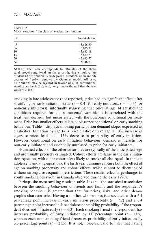
smoking in late adolescence (not reported), price had no significant effect afterstratifying by early initiation status (t ¼ 0.41 for early initiators, t ¼ �0.36 fornon-early initiators), informally suggesting that price at age 14 satisfies theconditions required for an instrumental variable: it is correlated with thetreatment decision but uncorrelated with the outcomes conditional on treat-ment. Price has smaller effects in late adolescence conditional on early smokingbehaviour. Table 4 displays smoking participation demand slopes expressed aselasticities. Initiation by age 14 is price elastic: on average, a 10% increase incigarette prices leads to a 13% decrease in probability of early initiation.However, conditional on early initiation behaviour, demand is inelastic fornon-early initiators and essentially unrelated to price for early initiators.

Estimated effects of the other covariates are typically of the anticipated signand are usually precisely estimated. Cohort effects are large in the early initia-tion equation, with older cohorts less likely to smoke all else equal. In the lateadolescent smoking equations, the birth year dummies capture both the effect ofage on smoking propensity and cohort effects, which cannot be disentangledwithout strong cross-equation restrictions. These results reflect large changes inyouth smoking behaviour in Canada observed during the early 1990s.

Perhaps the most striking result in table 3 is that the statistical associationbetween the smoking behaviour of friends and family and the respondent’ssmoking behaviour is greater than that for prices, risks, and other demo-graphic characteristics. Having a mother who smokes is associated with a 6.1percentage point increase in early initiation probability (t ¼ 7.2) and a 6.4percentage point increase in late adolescent smoking probability if the respon-dent does not initiate early (t ¼ 6.3). Each smoking friend the respondent hasincreases probability of early initiation by 1.0 percentage point (t ¼ 13.5),whereas each non-smoking friend decreases probability of early initiation by3.3 percentage points (t ¼ 21.5). It is not, however, valid to infer that having

TABLE 2Model selection from class of Student distributions

d.f. log-likelihood

5 �5,626.306 �5,635.3010 �5,663.1815 �5,682.2920 �5,693.771 �5,746.27

NOTES: Each row corresponds to estimates of the struc-tural model conditional on the errors having a multivariateStudent’s-t distribution listed degrees of freedom, where infinitedegrees of freedom denotes the Gaussian model. All listeddistributions may be rejected in favour of t5 at conventionalsignificance levels (2½L5 � L� � � 2

1 under the null that the truevalue of � is 5).

720 M.C. Auld

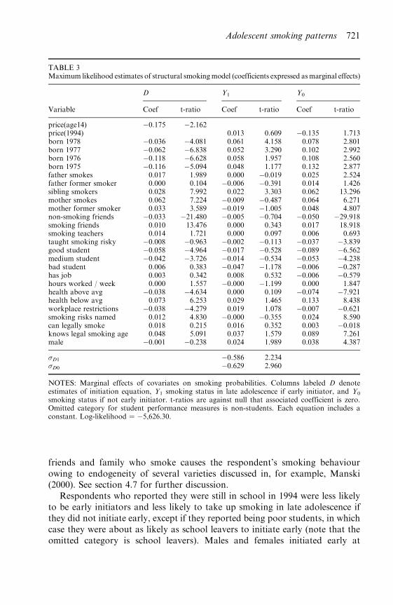
friends and family who smoke causes the respondent’s smoking behaviourowing to endogeneity of several varieties discussed in, for example, Manski(2000). See section 4.7 for further discussion.

Respondents who reported they were still in school in 1994 were less likelyto be early initiators and less likely to take up smoking in late adolescence ifthey did not initiate early, except if they reported being poor students, in whichcase they were about as likely as school leavers to initiate early (note that theomitted category is school leavers). Males and females initiated early at

TABLE 3Maximum likelihood estimates of structural smokingmodel (coefficients expressed asmarginal effects)

D Y1 Y0

Variable Coef t-ratio Coef t-ratio Coef t-ratio

price(age14) �0.175 �2.162price(1994) 0.013 0.609 �0.135 1.713born 1978 �0.036 �4.081 0.061 4.158 0.078 2.801born 1977 �0.062 �6.838 0.052 3.290 0.102 2.992born 1976 �0.118 �6.628 0.058 1.957 0.108 2.560born 1975 �0.116 �5.094 0.048 1.177 0.132 2.877father smokes 0.017 1.989 0.000 �0.019 0.025 2.524father former smoker 0.000 0.104 �0.006 �0.391 0.014 1.426sibling smokers 0.028 7.992 0.022 3.303 0.062 13.296mother smokes 0.062 7.224 �0.009 �0.487 0.064 6.271mother former smoker 0.033 3.589 �0.019 �1.005 0.048 4.807non-smoking friends �0.033 �21.480 �0.005 �0.704 �0.050 �29.918smoking friends 0.010 13.476 0.000 0.343 0.017 18.918smoking teachers 0.014 1.721 0.000 0.097 0.006 0.693taught smoking risky �0.008 �0.963 �0.002 �0.113 �0.037 �3.839good student �0.058 �4.964 �0.017 �0.528 �0.089 �6.562medium student �0.042 �3.726 �0.014 �0.534 �0.053 �4.238bad student 0.006 0.383 �0.047 �1.178 �0.006 �0.287has job 0.003 0.342 0.008 0.532 �0.006 �0.579hours worked / week 0.000 1.557 �0.000 �1.199 0.000 1.847health above avg �0.038 �4.634 0.000 0.109 �0.074 �7.921health below avg 0.073 6.253 0.029 1.465 0.133 8.438workplace restrictions �0.038 �4.279 0.019 1.078 �0.007 �0.621smoking risks named 0.012 4.830 �0.000 �0.355 0.024 8.590can legally smoke 0.018 0.215 0.016 0.352 0.003 �0.018knows legal smoking age 0.048 5.091 0.037 1.579 0.089 7.261male �0.001 �0.238 0.024 1.989 0.038 4.387

D1 �0.586 2.234D0 �0.629 2.960

NOTES: Marginal effects of covariates on smoking probabilities. Columns labeled D denoteestimates of initiation equation, Y1 smoking status in late adolescence if early initiator, and Y0

smoking status if not early initiator. t-ratios are against null that associated coefficient is zero.Omitted category for student performance measures is non-students. Each equation includes aconstant. Log-likelihood ¼ �5,626.30.


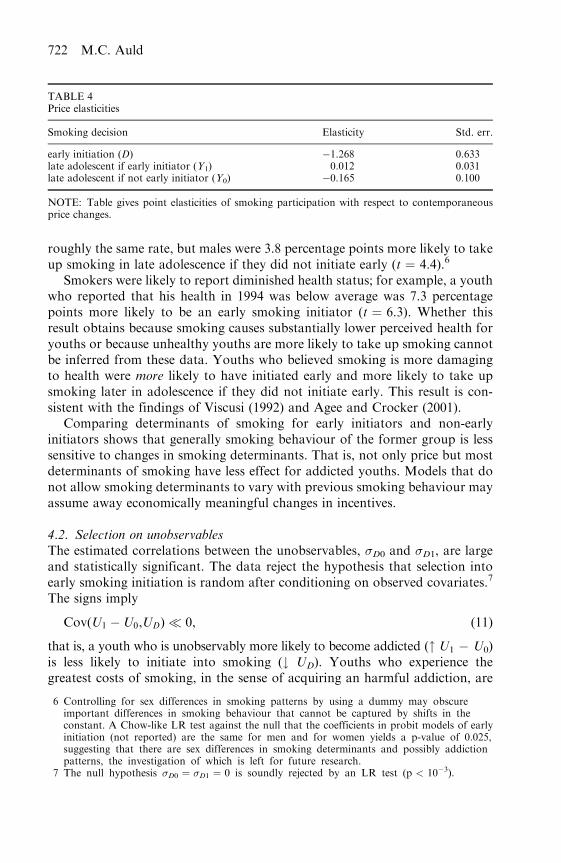
roughly the same rate, but males were 3.8 percentage points more likely to takeup smoking in late adolescence if they did not initiate early (t ¼ 4.4).6

Smokers were likely to report diminished health status; for example, a youthwho reported that his health in 1994 was below average was 7.3 percentagepoints more likely to be an early smoking initiator (t ¼ 6.3). Whether thisresult obtains because smoking causes substantially lower perceived health foryouths or because unhealthy youths are more likely to take up smoking cannotbe inferred from these data. Youths who believed smoking is more damagingto health were more likely to have initiated early and more likely to take upsmoking later in adolescence if they did not initiate early. This result is con-sistent with the findings of Viscusi (1992) and Agee and Crocker (2001).

Comparing determinants of smoking for early initiators and non-earlyinitiators shows that generally smoking behaviour of the former group is lesssensitive to changes in smoking determinants. That is, not only price but mostdeterminants of smoking have less effect for addicted youths. Models that donot allow smoking determinants to vary with previous smoking behaviour mayassume away economically meaningful changes in incentives.

4.2. Selection on unobservablesThe estimated correlations between the unobservables, D0 and D1, are largeand statistically significant. The data reject the hypothesis that selection intoearly smoking initiation is random after conditioning on observed covariates.7

The signs imply

Cov(U1 �U0,UD) � 0, (11)

that is, a youth who is unobservably more likely to become addicted (" U1 � U0)is less likely to initiate into smoking (# UD). Youths who experience thegreatest costs of smoking, in the sense of acquiring an harmful addiction, are

TABLE 4Price elasticities

Smoking decision Elasticity Std. err.

early initiation (D) �1.268 0.633late adolescent if early initiator (Y1) 0.012 0.031late adolescent if not early initiator (Y0) �0.165 0.100

NOTE: Table gives point elasticities of smoking participation with respect to contemporaneousprice changes.

6 Controlling for sex differences in smoking patterns by using a dummy may obscureimportant differences in smoking behaviour that cannot be captured by shifts in theconstant. A Chow-like LR test against the null that the coefficients in probit models of earlyinitiation (not reported) are the same for men and for women yields a p-value of 0.025,suggesting that there are sex differences in smoking determinants and possibly addictionpatterns, the investigation of which is left for future research.

7 The null hypothesis D0 ¼ D1 ¼ 0 is soundly rejected by an LR test (p < 10�3).

722 M.C. Auld

least likely to smoke, such that sample selection occurs in the anticipatedmanner. This result is consistent with the variants of the rational addictionmodel in which individuals have imperfect information on addictiveness andselect accordingly (Orphanides and Zervos 1995; Wang 1999).

4.3. Heterogeneous addictionThis section discusses the causal effect of early initiation on late adolescentsmoking probability. The causal effects of interest are means of Y1 � Y0 overdifferent conditioning sets, as discussed in, for example, Aakvik, Heckman,and Vytlacil (2005). Auld (2002) presents the expressions used to evaluate thecausal effect parameters for the multivariate Student model. In the presentcase, the causal effect may be considered to measure the level of addictivenessof smoking in the sense of Becker and Murphy (1988), who define an activityas addictive if increases in current consumption cause increases in futureconsumption.

As a baseline to contrast with the distributions of results calculated from thestructural model, simple conventional regression models were first estimated.Ordinary least squares estimates equation (3), where X includes the covariateslisted in table 3, yielded an estimate of � of 0.519 (t ¼ 48.11); that is, earlyinitiation is associated with a 52 percentage point increase in the probability oflate adolescent smoking. Probit regression produced similar results. Two-stageleast squares, instrumenting D with past price, gives an estimate of 0.463(t ¼ 0.90). This estimate ignores non-linearities in both stages, is difficult tointerpret when causal effects vary across respondents, and produces an impre-cise estimate because linear models are very sensitive to a lack of stronginstruments (the excluded instrument, price at age 14, has a t-statistic of�2.04 in the linear model). Conventional estimates, then, show that Y and Dare still highly correlated after being residualized with respect to observedcovariates and suggest that treating D as exogenous to Y overestimates thecausal effect of D on Y.

Table 5 summarizes the estimated distributions (induced by variation in X)of each causal effect calculated from the structural model. Standard errors and90% confidence intervals for the mean effects parameters were calculated usinga parametric bootstrap off the estimated asymptotic distribution of the struc-tural parameters; 1,000 bootstrap replications were used.

First, consider the average treatment effect for an individual with character-istics X,

ATE(X) ¼ E[Y1 � Y0jX]; (12)

the causal effect conditional on covariates averaged with respect to the dis-tribution of UD. The ATE measures how a randomly selected youth withcharacteristics X would respond to being forced to initiate early (or to beingprevented from initiating early). Table 5 shows that the mean of this effect –averaging over X and thus providing the empirical analogue of


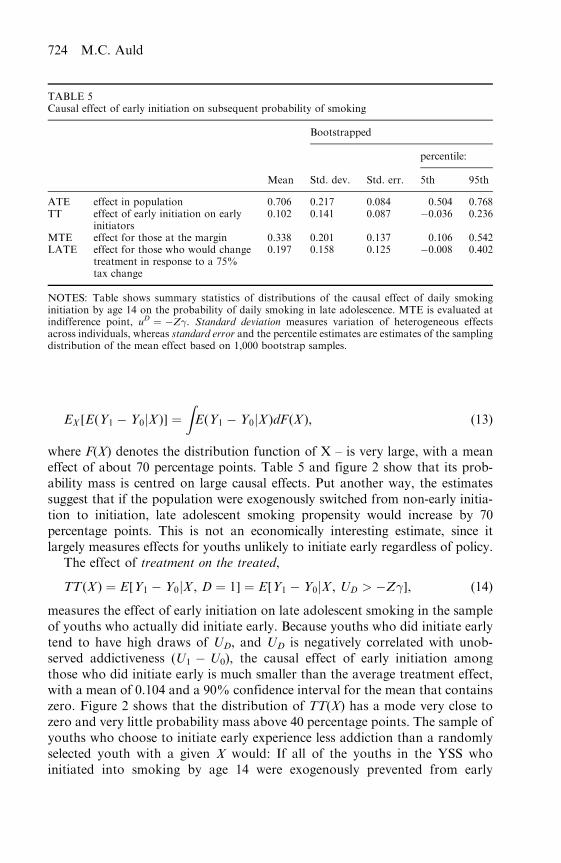
EX [E(Y1 � Y0jX)] ¼ZE(Y1 � Y0jX)dF(X), (13)

where F(X) denotes the distribution function of X – is very large, with a meaneffect of about 70 percentage points. Table 5 and figure 2 show that its prob-ability mass is centred on large causal effects. Put another way, the estimatessuggest that if the population were exogenously switched from non-early initia-tion to initiation, late adolescent smoking propensity would increase by 70percentage points. This is not an economically interesting estimate, since itlargely measures effects for youths unlikely to initiate early regardless of policy.

The effect of treatment on the treated,

TT(X) ¼ E[Y1 � Y0jX , D ¼ 1] ¼ E[Y1 � Y0jX , UD > �Z�], (14)

measures the effect of early initiation on late adolescent smoking in the sampleof youths who actually did initiate early. Because youths who did initiate earlytend to have high draws of UD, and UD is negatively correlated with unob-served addictiveness (U1 � U0), the causal effect of early initiation amongthose who did initiate early is much smaller than the average treatment effect,with a mean of 0.104 and a 90% confidence interval for the mean that containszero. Figure 2 shows that the distribution of TT(X) has a mode very close tozero and very little probability mass above 40 percentage points. The sample ofyouths who choose to initiate early experience less addiction than a randomlyselected youth with a given X would: If all of the youths in the YSS whoinitiated into smoking by age 14 were exogenously prevented from early

TABLE 5Causal effect of early initiation on subsequent probability of smoking

Bootstrapped

percentile:

Mean Std. dev. Std. err. 5th 95th

ATE effect in population 0.706 0.217 0.084 0.504 0.768TT effect of early initiation on early

initiators0.102 0.141 0.087 �0.036 0.236

MTE effect for those at the margin 0.338 0.201 0.137 0.106 0.542LATE effect for those who would change

treatment in response to a 75%tax change

0.197 0.158 0.125 �0.008 0.402

NOTES: Table shows summary statistics of distributions of the causal effect of daily smokinginitiation by age 14 on the probability of daily smoking in late adolescence. MTE is evaluated atindifference point, uD ¼ �Z�. Standard deviation measures variation of heterogeneous effectsacross individuals, whereas standard error and the percentile estimates are estimates of the samplingdistribution of the mean effect based on 1,000 bootstrap samples.

724 M.C. Auld

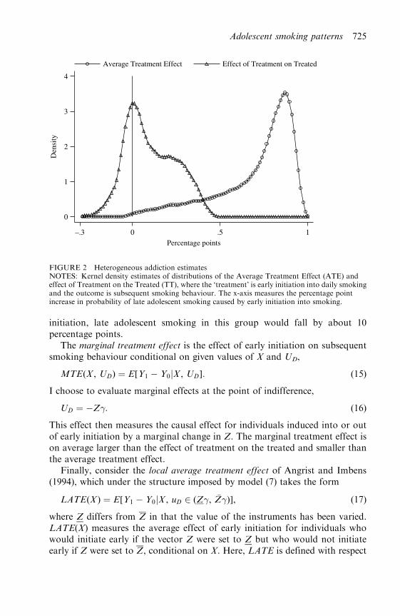
initiation, late adolescent smoking in this group would fall by about 10percentage points.

The marginal treatment effect is the effect of early initiation on subsequentsmoking behaviour conditional on given values of X and UD,

MTE(X , UD) ¼ E[Y1 � Y0jX , UD]: (15)

I choose to evaluate marginal effects at the point of indifference,

UD ¼ �Z�: (16)

This effect then measures the causal effect for individuals induced into or outof early initiation by a marginal change in Z. The marginal treatment effect ison average larger than the effect of treatment on the treated and smaller thanthe average treatment effect.

Finally, consider the local average treatment effect of Angrist and Imbens(1994), which under the structure imposed by model (7) takes the form

LATE(X) ¼ E[Y1 � Y0jX , uD 2 (Z�, �Z�)], (17)

where Z differs from Z in that the value of the instruments has been varied.LATE(X) measures the average effect of early initiation for individuals whowould initiate early if the vector Z were set to Z but who would not initiateearly if Z were set to Z, conditional on X. Here, LATE is defined with respect

Den

sity

Percentage points

Average Treatment Effect Effect of Treatment on Treated

–.3 0 .5 1

0

1

2

3

4

FIGURE 2 Heterogeneous addiction estimatesNOTES: Kernel density estimates of distributions of the Average Treatment Effect (ATE) andeffect of Treatment on the Treated (TT), where the ‘treatment’ is early initiation into daily smokingand the outcome is subsequent smoking behaviour. The x-axis measures the percentage pointincrease in probability of late adolescent smoking caused by early initiation into smoking.


to a 75% change in the price of tobacco faced at age 14. This LATE measuresthe average effect of early initiation on subsequent behaviour among youthswho would choose to initiate into smoking at observed prices but who wouldnot choose to initiate early if tobacco prices had been 75% higher. Table 5shows youths deferred from initiating into smoking by such a price increasewould exhibit an average 20% lower probability of smoking in late adolescenceas a result, holding the price of tobacco in late adolescence constant.

Table 6 breaks this result down by cohort. Older cohorts experience longerintervals of calendar time between age 14 and the time of measurement of theirsubsequent smoking behaviour. Therefore, we should expect older cohorts to beless influenced by their behaviour at age 14. Table 6 shows that each causal effectdecreases with cohort age, monotonically but for one exception. For example, theestimates suggest that youths who choose not to take up smoking by age 14because of a 75% tax increase would by 33.2 percentage points less likely tosmoke at age 15 but only 5.1 percentage points less likely to smoke at age 19. Theestimates suggest the effect of preventing youths from taking up smoking by age14 is largely temporary; smoking behaviour at onset of adulthood is similar towhat it would have been had early initiation not been prevented.

4.4. Effect of covariates on addictionObserved predictors of early initiation are quite similar to observed predictorsof subsequent smoking behaviour. The correlations between the predictedindexes are

Corr(Z�, X�0) ¼ 0:89

Corr(Z�, X�1) ¼ 0:42

Corr(X �0, X�1) ¼ 0:70: (18)

Observed characteristics that increase probability of early initiation also tendto increase probability of smoking in late adolescence regardless of whetherearly initiation occurs, and observed characteristics that lead to greater

TABLE 6Effect of initiation by age 14 on behaviour at ages 15 through 19

Born age in 1994 ATE TT MTE LATE

1979 15 0.735 0.240 0.465 0.3321978 16 0.753 0.147 0.473 0.2991977 17 0.710 0.034 0.318 0.1551976 18 0.684 �0.031 0.202 0.0791975 19 0.620 �0.046 0.160 0.051

NOTES: Table shows means of heterogenous causal effects of early smoking initiation on subsequentsmoking behaviour stratified by cohort. Cohorts born earlier experience longer periods of calendartime between early initiation and observation of subsequent smoking behaviour. LATE is defined withrespect to a 75% increase in cigarette prices. MTE is evaluated at indifference point, uD ¼ �Z�.

726 M.C. Auld

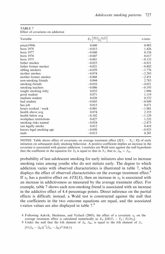
probability of late adolescent smoking for early initiators also tend to increasesmoking rates among youths who do not initiate early. The degree to whichaddiction varies with observed characteristics is illustrated in table 7, whichdisplays the effect of observed characteristics on the average treatment effect.8

If xk has a positive effect on ATE(X), then an increase in xk is associated withan increase in addictiveness as measured by the average treatment effect. Forexample, table 7 shows each non-smoking friend is associated with an increasein the addictive effect of 4.4 percentage points. Direct inference on the partialeffects is difficult; instead, a Wald test is constructed against the null thatthe coefficients in the two outcome equations are equal, and the associatedt-ratios values are also displayed in table 7.9

TABLE 7Effect of covariates on addiction

Variable EX@E(Y1�Y0jX)

@xk

h it-ratio

price(1994) 0.049 0.905born 1978 �0.015 1.426born 1977 �0.048 0.334born 1976 �0.047 0.617born 1975 �0.081 �0.133father smokes �0.025 �0.821father former smoker �0.021 �0.802sibling smokers �0.039 �1.776mother smokes �0.074 �2.295mother former smoker �0.068 �2.431non-smoking friends 0.044 2.783smoking friends �0.016 �4.021smoking teachers �0.006 �0.195taught smoking risky 0.035 1.096good student 0.071 1.119medium student 0.038 0.532bad student �0.043 �0.949has job 0.015 0.671hours worked / week �0.001 �1.901health above avg 0.074 2.355health below avg �0.102 �1.129workplace restrictions 0.027 1.232smoking risks named �0.024 �2.475can legally smoke 0.012 0.418knows legal smoking age �0.050 �0.925male �0.013 0.201

NOTES: Table shows effect of covariates on average treatment effect (E[Y1 � Y0 j X]) of earlyinitiation on subsequent daily smoking behaviour. A positive coefficient implies an increase in thecovariate is associated with greater addiction. t-statistics are Wald tests against the null hypothesisthat the coefficient in the equation for Y0 is equal to that in Y1; that is, �0k ¼ �1k.

8 Following Aakvik, Heckman, and Vytlacil (2005), the effect of a covariate xk on theaverage treatment effect is calculated numerically as EX [@E(Y1 � Y0 j X)/@xk].

9 Under the null that the kth element of �0, �0k, is equal to the kth element of �1,

[V(�1k � �0k)]�1

2(�1k � �0k)�aN(0,1).


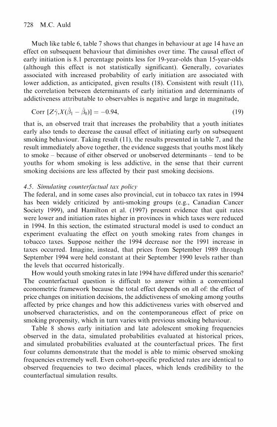
Much like table 6, table 7 shows that changes in behaviour at age 14 have aneffect on subsequent behaviour that diminishes over time. The causal effect ofearly initiation is 8.1 percentage points less for 19-year-olds than 15-year-olds(although this effect is not statistically significant). Generally, covariatesassociated with increased probability of early initiation are associated withlower addiction, as anticipated, given results (18). Consistent with result (11),the correlation between determinants of early initiation and determinants ofaddictiveness attributable to observables is negative and large in magnitude,

Corr [Z�,X(�1 � �0)] ¼ �0:94, (19)

that is, an observed trait that increases the probability that a youth initiatesearly also tends to decrease the causal effect of initiating early on subsequentsmoking behaviour. Taking result (11), the results presented in table 7, and theresult immediately above together, the evidence suggests that youths most likelyto smoke – because of either observed or unobserved determinants – tend to beyouths for whom smoking is less addictive, in the sense that their currentsmoking decisions are less affected by their past smoking decisions.

4.5. Simulating counterfactual tax policyThe federal, and in some cases also provincial, cut in tobacco tax rates in 1994has been widely criticized by anti-smoking groups (e.g., Canadian CancerSociety 1999), and Hamilton et al. (1997) present evidence that quit rateswere lower and initiation rates higher in provinces in which taxes were reducedin 1994. In this section, the estimated structural model is used to conduct anexperiment evaluating the effect on youth smoking rates from changes intobacco taxes. Suppose neither the 1994 decrease nor the 1991 increase intaxes occurred. Imagine, instead, that prices from September 1989 throughSeptember 1994 were held constant at their September 1990 levels rather thanthe levels that occurred historically.

Howwould youth smoking rates in late 1994 have differed under this scenario?The counterfactual question is difficult to answer within a conventionaleconometric framework because the total effect depends on all of: the effect ofprice changes on initiation decisions, the addictiveness of smoking among youthsaffected by price changes and how this addictiveness varies with observed andunobserved characteristics, and on the contemporaneous effect of price onsmoking propensity, which in turn varies with previous smoking behaviour.

Table 8 shows early initiation and late adolescent smoking frequenciesobserved in the data, simulated probabilities evaluated at historical prices,and simulated probabilities evaluated at the counterfactual prices. The firstfour columns demonstrate that the model is able to mimic observed smokingfrequencies extremely well. Even cohort-specific predicted rates are identical toobserved frequencies to two decimal places, which lends credibility to thecounterfactual simulation results.

728 M.C. Auld

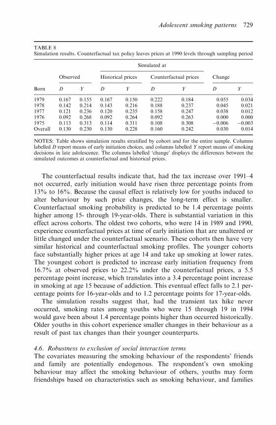
The counterfactual results indicate that, had the tax increase over 1991–4not occurred, early initiation would have risen three percentage points from13% to 16%. Because the causal effect is relatively low for youths induced toalter behaviour by such price changes, the long-term effect is smaller.Counterfactual smoking probability is predicted to be 1.4 percentage pointshigher among 15- through 19-year-olds. There is substantial variation in thiseffect across cohorts. The oldest two cohorts, who were 14 in 1989 and 1990,experience counterfactual prices at time of early initiation that are unaltered orlittle changed under the counterfactual scenario. These cohorts then have verysimilar historical and counterfactual smoking profiles. The younger cohortsface substantially higher prices at age 14 and take up smoking at lower rates.The youngest cohort is predicted to increase early initiation frequency from16.7% at observed prices to 22.2% under the counterfactual prices, a 5.5percentage point increase, which translates into a 3.4 percentage point increasein smoking at age 15 because of addiction. This eventual effect falls to 2.1 per-centage points for 16-year-olds and to 1.2 percentage points for 17-year-olds.

The simulation results suggest that, had the transient tax hike neveroccurred, smoking rates among youths who were 15 through 19 in 1994would gave been about 1.4 percentage points higher than occurred historically.Older youths in this cohort experience smaller changes in their behaviour as aresult of past tax changes than their younger counterparts.

4.6. Robustness to exclusion of social interaction termsThe covariates measuring the smoking behaviour of the respondents’ friendsand family are potentially endogenous. The respondent’s own smokingbehaviour may affect the smoking behaviour of others, youths may formfriendships based on characteristics such as smoking behaviour, and families

TABLE 8Simulation results. Counterfactual tax policy leaves prices at 1990 levels through sampling period

Simulated at

Observed Historical prices Counterfactual prices Change

Born D Y D Y D Y D Y

1979 0.167 0.155 0.167 0.150 0.222 0.184 0.055 0.0341978 0.142 0.214 0.143 0.216 0.188 0.237 0.045 0.0211977 0.121 0.236 0.120 0.235 0.158 0.247 0.038 0.0121976 0.092 0.268 0.092 0.264 0.092 0.263 0.000 0.0001975 0.113 0.313 0.114 0.311 0.108 0.308 �0.006 �0.003Overall 0.130 0.230 0.130 0.228 0.160 0.242 0.030 0.014

NOTES: Table shows simulation results stratified by cohort and for the entire sample. Columnslabelled D report means of early initiation choices, and columns labelled Y report means of smokingdecisions in late adolescence. The columns labelled ‘change’ displays the differences between thesimulated outcomes at counterfactual and historical prices.


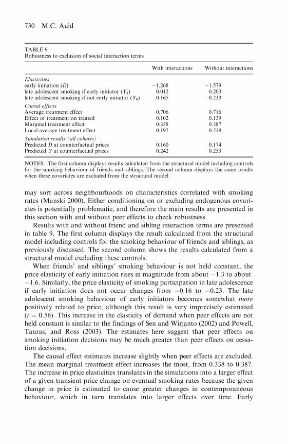
may sort across neighbourhoods on characteristics correlated with smokingrates (Manski 2000). Either conditioning on or excluding endogenous covari-ates is potentially problematic, and therefore the main results are presented inthis section with and without peer effects to check robustness.

Results with and without friend and sibling interaction terms are presentedin table 9. The first column displays the result calculated from the structuralmodel including controls for the smoking behaviour of friends and siblings, aspreviously discussed. The second column shows the results calculated from astructural model excluding these controls.

When friends’ and siblings’ smoking behaviour is not held constant, theprice elasticity of early initiation rises in magnitude from about �1.3 to about�1.6. Similarly, the price elasticity of smoking participation in late adolescenceif early initiation does not occur changes from �0.16 to �0.23. The lateadolescent smoking behaviour of early initiators becomes somewhat morepositively related to price, although this result is very imprecisely estimated(t ¼ 0.56). This increase in the elasticity of demand when peer effects are notheld constant is similar to the findings of Sen and Wirjanto (2002) and Powell,Tauras, and Ross (2003). The estimates here suggest that peer effects onsmoking initiation decisions may be much greater than peer effects on cessa-tion decisions.

The causal effect estimates increase slightly when peer effects are excluded.The mean marginal treatment effect increases the most, from 0.338 to 0.387.The increase in price elasticities translates in the simulations into a larger effectof a given transient price change on eventual smoking rates because the givenchange in price is estimated to cause greater changes in contemporaneousbehaviour, which in turn translates into larger effects over time. Early

TABLE 9Robustness to exclusion of social interaction terms

With interactions Without interactions

Elasticitiesearly initiation (D) �1.268 �1.579late adolescent smoking if early initiator (Y1) 0.012 0.203late adolescent smoking if not early initiator (Y0) �0.165 �0.233

Causal effectsAverage treatment effect 0.706 0.716Effect of treatment on treated 0.102 0.139Marginal treatment effect 0.338 0.387Local average treatment effect 0.197 0.219

Simulation results (all cohorts)Predicted D at counterfactual prices 0.160 0.174Predicted Y at counterfactual prices 0.242 0.253

NOTES: The first column displays results calculated from the structural model including controlsfor the smoking behaviour of friends and siblings. The second column displays the same resultswhen these covariates are excluded from the structural model.

730 M.C. Auld

initiation frequency at (lower) counterfactual prices rises from 0.160 in themodel with peer effects to 0.174 in the model excluding peer effects, and thechange in overall smoking rates is predicted to be 2.5 percentage points, asopposed to 1.4 points in the model without peer effects.

Overall, the major results are very similar with and without conditioningon the behaviour of friends and family. When such behaviour is not heldconstant, youths are estimated to exhibit greater response to price changesand the addictive effect of past behaviour on current behaviour increasesmodestly.

5. Conclusions

Correlation over time in smoking behaviour could be attributable to either acausal effect of past on current smoking (i.e., an addictive effect) or correlationover time in tastes and other incentives to smoke. Preventing youth smokingwill only reduce adult smoking rates to the extent that this correlation reflectscausality. In this paper an econometric model was developed and estimated tomeasure causality over time in the smoking behaviour of Canadian youths inthe 1990s, paying particular attention to the theoretical prediction that addic-tiveness varies across people, and therefore marginal youths whose smokingpatterns are changed by policy may experience different addictive effects thanother youths.

The results suggest that smoking is addictive for almost all youths.However, youths who do start smoking early or who are likely to be preventedor induced to take up smoking early by policy changes experience a muchsmaller addictive effect than other youths. The average youth in the popula-tion, for example, experiences an increase in the probability of late adolescentsmoking of 71 percentage points if she is exogenously induced to initiatesmoking early. However, this effect is only 20 percentage points in the sub-population of marginal youths who would change their smoking status inresponse to a 75% change in tobacco prices. Further, the marginal causaleffect of smoking at age 14 on subsequent smoking behaviour diminishesrapidly with age, essentially vanishing by age 19. Consistent with the resultsof Glied (2002), the estimates suggest that policies that deter early initiationwill not have large effects on eventual smoking rates.

The estimated structural model suggests that initiation decisions in earlyadolescence are price sensitive (with an elasticity of �1.3), but that, conditionalon early smoking status, later decisions are little affected by price. The modelfurther reveals that smoking is less sensitive to changes in incentives other thanprice for addicted youths. If social interaction effects are excluded from themodel, the price elasticity of smoking initiation markedly increases in magni-tude, but, conditional on previous initiation, smoking propensity is inelasticeven when peer behaviour is not held constant.


Appendix: The likelihood function

The observed outcomes for an individual are (Y, D, X, Z). Given the structureimposed by equations (7) and (8) and the assumption that the errors U aredistributed multivariate Student’s t, the contributions to the likelihood take theform of bivariate integrals over the Student density. For example, conditionalon degrees of freedom �, the probability of observing the event (D ¼ 1,Y ¼ 1), given (X,Z) (suppressing subscripting for individuals), is

Pr (D ¼ 1, Y ¼ 1jX , Z, �) ¼Z1

�Z�

Z1

�X�1

t�(s; �D1)ds,

where SD1 denotes the 2 � 2 covariance matrix of (UD,U1) and t�(�) denotesthe bivariate Student density with degrees of freedom �, as given by equation(9) in the text. This expression follows from the properties of the multivariateStudent distribution; see Johnson and Kotz (1972).

The likelihood function conditional on � can be expressed

L ¼Y

D ¼ 0,Y0 ¼ 0

Z�Z�

�1

Z�X�0

�1

t�(s; �D0)ds

xY

D ¼ 0,Y0 ¼ 1

Z�Z�

�1

Z1

�X�0

t�(s; �D0)ds

xY

D ¼ 1,Y1 ¼ 0

Z1

�Z�

Z�X�1

�1

t�(s; �D1)ds

xY

D ¼ 1,Y1 ¼ 1

Z1

�Z�

Z1

�X�1

t�(s; �D1)ds,

(20)

where SDj denotes the 2 � 2 covariance matrix of (UD,Uj).

References

Aakvik, A., J. Heckman, and E. Vytlacil (2005) ‘Estimating treatment effects fordiscrete outcomes when responses to treatment vary: an application to Norwegianvocational rehabilitation programs,’ Journal of Econometrics 125, 15–51

Agee, M., and T. Crocker (2001) ‘Smoking parents’ evaluation of their own andchildrens’ health,’ manuscript

Angrist, J., G. Imbens, and D. Rubin (1996) ‘Identification of causal effects usinginstrumental variables,’ Journal of the American Statistical Association 91, 444–55

Ary, D., and A. Biglan (1988) ‘Longitudinal changes in adolescent cigarette smokingbehavior: onset and cessation,’ Journal of Behavioral Medicine 11, 361–82

732 M.C. Auld

Auld, M. (2002) ‘Robust system estimation of causal effects on binary outcomes withapplication to effect of alcohol abuse on employment,’ manuscript

Canadian Cancer Society, Non-smokers’ Rights Association, Physicians for a Smoke-free Canada, and Quebec Coalition for Tobacco Control (1999) ‘Surveying thedamage: cut-rate tobacco products and public health in the 1990s,’ manuscript

Becker, G., and K. Murphy (1988) ‘A theory of rational addiction,’ Journal of PoliticalEconomy 96, 675–700

Chib, S., and B. Hamilton (2001) ‘Bayesian analysis of cross-section and clusteredtreatment models,’ Journal of Econometrics 97, 25–50

Clayton, R., A. Cattarelo, and B. Johnstone (1996) ‘The effectiveness of Drug AbuseResistance Education (Project DARE): 5-year follow-up results,’ PreventativeMedicine 25, 3–7–318

DeCicca, P., D. Kenkel, A. Mathios (2002) ‘Putting out the fires: will higher taxesreduce the onset of youth smoking?’ Journal of Political Economy 110, 144–69

Evans, W., and L. Huang (1998) ‘Cigarette taxes and teen smoking: New evidence frompanels of repeated cross-sections,’ working paper, University of Maryland

Genz, A., and F. Bretz (2002) ‘Comparison of methods for the computation of multi-variate t probabilities,’ Journal of Computational and Graphical Statistics, 11, 950–71

Gilleskie, D., and K. Strumpf (2000) ‘The behavioral dynamics of youth smoking,’National Bureau of Economic Research Working Paper No. 7838

Glied, S. (2002) ‘Youth tobacco control: Reconciling theory and empirical evidence,’Journal of Health Economics 21, 117–35

Goldberger, A. (1983) ‘Abnormal selection bias,’ in Studies in Econometrics, TimeSeries, and Multivariate Statistics, ed. S. Karlin, T. Amemiya, and L. Goodman(New York: Academic Press)

Gruber, J. (2000) ‘Youth smoking in the U.S.: prices and policies,’ National Bureau ofEconomic Research Working Paper No. 7506

Hamilton, V., C. Levington, Y. St-Piere, and F. Grimard (1997) ‘The effect of tobaccotax cuts on cigarette smoking in Canada,’ Canadian Medical Association Journal 156,187–91

Harris, J. and S. Chan (1999) ‘The continuum of addiction: cigarette smoking inrelation to price among Americans aged 15–29,’ Health Economics 8, 81–6

Heckman, J. (1997) ‘Instrumental variables: a study of implicit behavioral assumptionsused in making program evaluations,’ Journal of Human Resources 32, 441–62

Heckman, J., J. Tobias, and E. Vytlacil (2000) ‘Simple estimators for treatment para-meters in a latent variable framework,’ Review of Economics and Statistics 85, 748–55

Imbens, G., and J. Angrist (1994), ‘Identification and estimation of local averagetreatment effects,’ Econometrica 62, 467–75

Imbens, G., and D. Rubin (1997) ‘Bayesian inference for causal effects in randomizedexperiments with noncompliance,’ Annals of Statistics 25, 305–27

Johnson, N., and S. Kotz (1972) Distribution in Statistics (New York: Wiley)Jones, A., and M. Forster (2001) ‘The role of taxes in starting and quitting smoking:

duration analysis of British data,’ Journal of the Royal Statistical Society: Series A164, 517–47

Kenkel, D., D. Lillard, and A. Mathios (2003) ‘Smoke or fog: the usefulness ofretrospectively reported information about smoking,’ Addiction 98, 1307–14

Krauth, B. (2001) ‘Peers and prices: Explaining the black/white youth smoking gap,’manuscript, Simon Fraser University

Manski, C. (2000) ‘Economic analysis of social interactions,’ Journal of EconomicPerspectives 14, 115–36

Orphanides, A. and D. Zervos (1995) ‘Rational addiction with learning and regret,’Journal of Political Economy 103, 739–58


Powell, L., J. Tauras, and H. Ross (2003) ‘The importance of peer effects, cigaretteprices, and tobacco control policies for youth smoking behavior,’ working paper,University of Illinois at Chicago

Sen, A., and T. Wirjanto (2003) ‘Social interactions, taxes, and youth smoking,’ work-ing paper, University of Waterloo

Statistics Canada (1996) ‘Microdata user’s guide: Youth Smoking Survey 1994,’ mimeoTauras, J., and F. Chaloupka (1999) ‘Determinants of smoking cessation: an analysis of

young adult men and women,’ National Bureau of Economic Research WorkingPaper No. 7262

Tauras, J., P. O’Malley and L. Johnston (2001) ‘Effects of price and access laws onteenage smoking initiation: a national longitudinal analysis,’ National Bureau ofEconomic Research Working Paper No. 8331

Viscusi, K. (1992) Smoking: Making the Risky Decision (Oxford: Oxford UniversityPress)

Wang, R. (1999) ‘The optimal consumption and quitting of harmful addictive goods,’working paper, Queen’s University

Williams, J. (2004) ‘Habit formation and college students’ demand for alcohol,’ HealthEconomics, forthcoming

734 M.C. Auld

Long term effects of tobacco prices faced byadolescents

M. Christopher AuldDepartment of Economics

University of [email protected]

Mahmood ZarrabiFaculty of Medicine

University of [email protected]

Abstract

We estimate the effects of tobacco prices faced in adolescence on smoking patternsof adults aged 19 to 40. Use of large repeated cross–sectional surveys in Canada inthe early 2000s allows us to exploit substantial and plausibly exogenous tax changesacross time and regions which occurred roughly a decade earlier. Results from avariety of econometric techniques suggest that there is a small but detectablelong–run effect of price faced during adolescence. A 10% increase in prices facedduring adolescence, holding contemporaneous prices constant, leads to at mosta 1% reduction in smoking propensity and intensity in early to mid adulthood,and we cannot reliably reject the hypothesis that the long term effect is zero.The results are sensitive to specification and to how price during adolescence ismeasured.

JEL Classification: I12, I18, C2Keywords: smoking, addiction, tobacco tax, adolescents.

Acknowledgements. Auld thanks the Alberta Heritage Foundation for MedicalResearch (AHFMR) for financial support. Herb Emery, Dan Gordon, MingshanLu, and seminar participants at the 2008 Canadian Economics Association meet-ings and at the University of Calgary provided helpful comments. Both authorsthank Statistics Canada for providing access to confidential data.

mailto:[email protected]

mailto: [email protected]

Long Term Effects of Tobacco Prices Facedby Adolescents

1 Introduction.

A policy intervention deters a youth from initiating into smoking. Does the intervention

merely defer initiation, such that the youth will become an adult smoker, or is initiation

deterred? The efficacy of policies targeted at reducing youth smoking hinges on this

question, yet little relevant evidence has been presented in the literature. In this paper

we contribute by estimating the long–run effects of changes in tobacco taxation policy.

Our empirical strategy is designed to exploit large changes in cigarette prices in Canada

from 1991 to 1994. We use data from repeated waves of the Canadian Community Health

Survey (CCHS) data drawn from 2001, 2003 and 2005 to study changes in smoking

status as various cohorts faced highly variable prices at peak initiation ages. Our major

finding is that high prices faced during adolescence exert a small but detectable effect

on smoking patterns later in life: A 10% increase in average cigarette prices faced over

ages 12 through 18 leads to a one percentage point reduction in probability of daily

smoking in adulthood. We show that these results depend on econometric specification,

in particular, that previous studies which focused on price faced at age 14 rather than

over a larger span of adolescence may find misleading small effects.

We are particularly interested in the long–run effect of taxation. Other smoking

control policies such as clean indoor air laws, restrictions on cigarette use for the youth,

and health warnings, may be effective, but taxation is widely considered to be the most

1

effective policy instrument (Warner et al., 1995). A substantial empirical literature on

youth demand typically finds that youth price elasticities are much larger than adult

elasticities.1 It is tempting to conclude that high youth elasticities directly imply that

taxation is an effective control policy. However, if high taxes faced in youth defer instead

of deter initiation, the long run effects will be small even when contemporaneous effects

are large.

High youth elasticities with no long–run effect will occur if correlation in smoking

behavior over time is not due to a causal effect of past smoking on current smoking, but

can rather be attributed to persistence in preferences, peer and social influences, and

contextual effects over time. The literature, conversely, sometimes interprets correlation

between youth smoking outcomes and adult smoking outcomes as evidence of a causal

effect of youth smoking on adult smoking. For example, Paul et al. (2009) find that 14 or

15 year olds who report having experimented with cigarettes are 2.72 times more likely

to report daily smoking two decades later than counterparts who had not experimented.

The authors conclude that reducing experimentation will, therefore, reduce adult smok-

ing. However, the set of youths who choose to experiment is not randomly selected, and

it is possible that reducing experimentation will have less effect than anticipated, or even

no effect, even given that experimentation and early initiation predict higher smoking

propensity much later in life. In the terminology of Becker and Murphy (1988), a causal

effect of past smoking on current smoking for a given person means by definition that

smoking is addictive for that person. If smoking is an addictive behavior in this sense,

then policies which reduce smoking in youth will cause reduced smoking in adulthood.

Conversely, if smoking is not addictive, then policies which reduce youth smoking will

1Carpenter and Cook (2008); Cawley et al. (2004); Harris and Chan (1999); Lewitt and Grossman(1981); Tauras and Chaloupka (1999). However, DeCicca et al. (2008) argue that the “conventionalwisdom may have it exactly backwards” as their results suggest youth smoking initiation is very inelasticand cessation only moderately elastic. Similarly, Sen and Wirjanto (2009) use Canadian data spanningthe tax shocks we also exploit in this paper to show that youth smoking elasticities are modest, around0.10 to 0.14, much lower than reported by previous studies.

2

have no effect, other things equal, on adult smoking. Correlations between youth and

adult smoking patterns generally cannot disentangle causation from correlation.

Previous studies conclude that the long–run effect is small. Auld (2005) estimates a

model in which past smoking is interpreted as an endogenously assigned treatment on

current smoking. Auld shows that marginal smokers are less influenced by past smoking

than average smokers, and in part due to this heterogeneity the causal effect of past

on current smoking diminishes rapidly with age. However, Auld only studies smoking

behavior up to age 19. Gilleskie and Strumpf (2005) treat lagged cigarette consumption

as an endogenous regressor in adolescent cigarette demand models and, similarly, find

past consumption causes current consumption. Glied (2002, 2003) presents estimates of

the effect of price faced at age 14 on adult smoking behavior using the NLSY79 panel.

Glied finds that the effect at age 30 is less than half the contemporaneous effect and

the effect at age 40 is essentially zero. Similarly, Gruber and Zinman (2001) finds that,

in a sample of pregnant women, the effect of taxes at ages 14 through 17 is reduced to

about 25% of the contemporaneous effect by age 24. Eisenberg and Rowe (2009) use the

Vietnam draft lottery as a natural experiment to study the effect of smoking in early

adulthood (age 19 to 22) on smoking later in life. They show military service increases

contemporaneous smoking propensity by 35 percentage points, but this effect dwindles

to 11 percentage points by age 25 to 30 and to essentially nothing by ages 45 to 55. Thus,

the small body of literature to date on long smoking dynamics unanimously suggests

that prior smoking does not substantially cause current smoking over the medium to

long run.

We contribute to this literature in several ways. Our basic approach is similar to

that of Glied (2002): we estimate models of adult smoking in which we include prices

faced during adolescence as covariates. We use Canadian data from 2001 through 2005,

an ideal sampling period for our purposes since very large tax changes across time and

3

regions in Canada roughly a decade prior give us large variation in past price. Our

data are less informative per respondent than those of previous studies using panels

because we cannot control in detail for time–varying characteristics during youth, nor

do we observe region of residence during youth, but our cross–sections provide about

an order of magnitude more observations than are available in most panels. We address

the issue that, theoretically, every past price ought to affect current smoking patterns in

more detail than previous work by assessing the sensitivity of the estimates to various

different measures of youth prices. Finally, we study both participation decisions and

intensity of smoking.

2 Data.

2.1 The Canadian Community Health Survey.

The CCHS is a cross-sectional survey conducted biannually by Statistics Canada since

2001. The CCHS collects information on health status, health care utilization, and

health determinants for the Canadian population. We use the first three cycles, 2001,

2003, and 2005. We restrict the sample to young adults (aged 19 through 40) because

tobacco taxes in Canada exhibited little variation until the early 1990s, so price faced

as youths exhibits little variation for older respondents. Further, we use retrospective

information on smoking experimentation and initiation, and recall bias is presumably

more of a problem as the time interval increases (Kenkel et al., 2004). The key advantages

of using CCHS data are that first, the CCHS sample sizes are large. Since we restrict the

sample to young adults, smaller datasets, including panels, would not provide sufficient

observations. Second, the sampling window 2001 through 2005 occurs roughly a decade

after large Federal and provincial changes in taxes that occurred in 1991 through 1994,

so that we have substantial variation in lagged prices.

4

The CCHS provides rich data on smoking patterns and retrospective questions on

smoking history. We use retrospective information on experimentation as measured by

age at which the respondent reports first smoking a whole cigarette and age at initiation

into daily smoking. Contemporaneous smoking patterns are captured by an indicator for

daily smoking, number of cigarettes smoked per day for daily smokers, and an indicator

for former daily smoking. A person is considered as a daily smoker if he smoked each day

in the month prior to the interview. A former smoker has smoked at least 100 cigarettes

in his life but does not currently smoke. A never-smoker is neither a current nor former

smoker.

Table 1 displays descriptive statistics for the key variables. The ethnicity of a respon-

dent is ascertained from a question addressing his country of birth. Immigration status

is derived based on his current age and year of landing in Canada. If the respondent’s

age upon landing in Canada was less than 12, we set an immigrant dummy to unity. If

the respondent was older than 12, we cannot observe the relevant youth price cleanly and

drop the observation. Socioeconomic variation is captured by a set of dummy variables

indicating educational levels and a set of dummies indicating household income ranges.

Finally, we include indicators for marital status and pregnancy.

2.2 Tobacco taxation in Canada.

Tobacco taxes in Canada in the early 1990s were highly variable. A large Federal tax

increase in 1991 substantially raised prices over the previous year. The price of a carton

of 200 cigarettes rose from roughly $35 in 1990 to almost $50 in 1991. Studlar (2002)

notes that Canadian tobacco taxes from 1984 to 1991 quadrupled while American taxes

increased by less than 50%—taxes in Canada averaged about seven times the U.S. level.

Prices remained uniformly high until 1994. By 1994 concern over smuggling across

the U.S. border resulting from the tax–induced price differential lead to a $14 to $21

5

reduction in the price of a pack of 200 cigarettes in Ontario, Quebec, New Brunswick,

Prince Edward Island, and Novo Scotia, whereas the price of cigarettes remain relatively

high in the Western provinces and in Newfoundland. These large changes in price over

time and regions were not the result of regional health concerns over smoking and can

be considered exogenous to smoking decisions (Hamilton et al., 1997).

Theory suggests the entire sequence of past (and in some models, future) prices

affect current smoking patterns (Becker and Murphy, 1988). Empirical models must

make simplifying assumptions in the interest of tractability. Previous research on long–

run tax effects focuses on prices faced at age 14, the peak of the hazard into smoking. We

investigate the robustness of this simplification by contrasting several different notions

of “price faced during adolescence:”

1. Cigarette price at age 14.

2. Average cigarette price over ages 14 through 16.

3. Average cigarette price over ages 12 through 18.

Figure 1 displays cigarette prices faced by CCHS respondents when they were age

14 against their age at the time of the CCHS interview. Relatively young respondents

tended to face high prices, and the 1991 through 1994 period of particularly high prices

can be observed as a “bump” in price faced at age 14 for respondents in roughly their

late twenties at the time of the CCHS interviews. Also apparent in the graph is high

variability across provinces for respondents in their early twenties, and little variation

across time or provinces for respondents in their mid to late thirties.

Averaging over longer age spans smoothes the price series. Since price at ages other

than 14 affects initiation and cessation behavior, using price at age 14 and ignoring

prices at other ages may introduce a substantial omitted variables problem. We assess

how sensitive estimates are to these various price measures. We use the consumer price

6

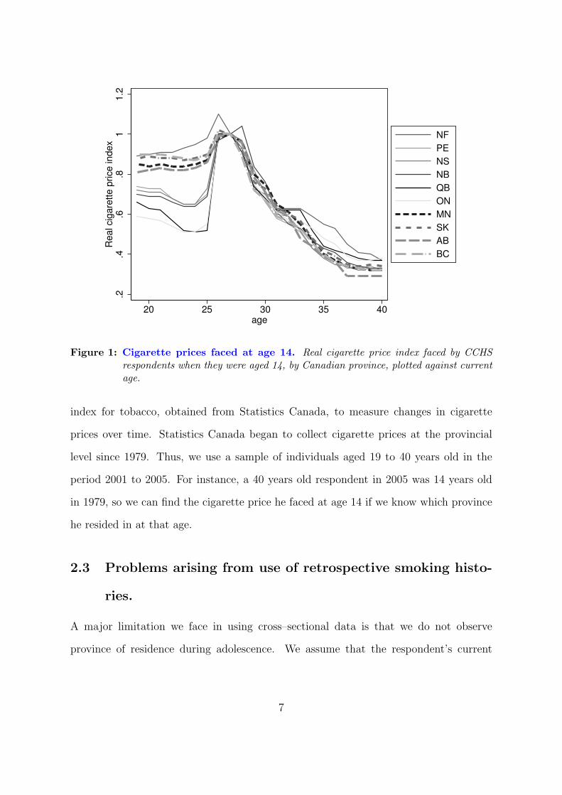
.2.4

.6.8

11

.2R

ea

l cig

are

tte

price

in

de

x

20 25 30 35 40age

NF

PE

NS

NB

QB

ON

MN

SK

AB

BC

Figure 1: Cigarette prices faced at age 14. Real cigarette price index faced by CCHSrespondents when they were aged 14, by Canadian province, plotted against currentage.

index for tobacco, obtained from Statistics Canada, to measure changes in cigarette

prices over time. Statistics Canada began to collect cigarette prices at the provincial

level since 1979. Thus, we use a sample of individuals aged 19 to 40 years old in the

period 2001 to 2005. For instance, a 40 years old respondent in 2005 was 14 years old

in 1979, so we can find the cigarette price he faced at age 14 if we know which province

he resided in at that age.

2.3 Problems arising from use of retrospective smoking histo-

ries.

A major limitation we face in using cross–sectional data is that we do not observe

province of residence during adolescence. We assume that the respondent’s current

7

province of residence was also his province of residence during adolescence, thus intro-

ducing measurement error. The resulting bias is likely to be small. First, from 1995

to 2004 a calculation by the authors using the longitudinal National Population Health

Survey in Canada shows roughly 10% of the respondents aged 12 to 40 years old in

1994 had moved across the provinces from 1994 to 2003. Second, although cigarette

prices in Canada have varied substantially over time, there was not much disparity in

the prices across the provinces during the period 1979-1994 (as can be seen in Figure 1).

Third, prices across provinces are spatially correlated and moves are more likely to be to

nearby than distant provinces. Finally, to assuage remaining concern, we conducted a

small Monte Carlo experiment to make a crude assessment of the magnitude of the bias

given the features of our data. More details are provided in the Appendix. Ignoring the

other two mitigating factors and focusing just on random assignment of price for the

10% of movers in our sample, we find the relative bias introduced by measurement error

is about 10%. The expected ratio of estimated price coefficients using real prices (βtrue)

to coefficients estimated when 10% of prices are randomly assigned (βerror) is estimated

as

E

[βerror

βtrue

]≈ 0.900. (1)

This is not a surprising result since textbook results tell us the ratio of the limit of our

estimator using mismeasured covariates to the limit using the true covariates is equal

to the proportion of variance in the mismeasured covariate attributable to variation in

the true covariate, but it is not obvious how much of the variability in observed prices

is due to noise from unobserved cross-province moves, and the simulation serves as an

illustration of the magnitude of the effect.2 For the reasons above the realized bias in

our sample is likely to be smaller still. Since our sample of roughly 95,000 observations

2That is, if σ2x is the variance of the covariate in a univariate model and σ2

ε is the variance of themeasurement error, then βerror

βtrue→ σ2

x

σ2x+σ

2ε.

8

implies our standard errors will be roughly three times smaller than comparable esti-

mates using one–tenth as many observations, as we might be able to construct using a

panel such as the NLSY, we view the cost of the modest attenuation bias introduced by

our inability to observe province of residence during adolescence to be smaller than the

benefit of increased precision. Nonetheless, we interpret our estimates keeping in mind

that they are slightly biased towards zero.

3 Methods.

The econometric goal is to estimate the effect of youth prices on adult smoking pat-

terns as measured by an indicator for daily smoking and, conditional on daily smoking,

number of cigarettes per day. As part of our empirical strategy, we also estimate the

contemporaneous effect of youth prices on age of experimentation, age of initiation, and

the probability of initiation during adolescence.

Following Auld (2005), we have in mind an underlying structural model of dynamic

smoking decisions of the form,

S0 = X0β0 + θ0P0 + u0 (2)

S1 = X1β1 + θ1P1 + δS0 + u1, (3)

where subscript 0s denote observations during adolescence and subscript 1s adult out-

comes, S is a measure of smoking status, X are vectors of covariates, P is tobacco prices,

u are error terms, and {β, θ, δ} are conformable vectors of unknown parameters. Our

goal here is not to recover estimates of the causal effect of past smoking on current

smoking (δ), so we avoid all of the issues that arise in estimation of simultaneous equa-

tions by estimating reduced forms. Equation (2) is estimable subject to the limitation

that we do not observe time–varying characteristics during youth X0. However, many

9

of the characteristics we condition on do not vary over time, and others (such as edu-

cation and household income) can be considered to proxy characteristics during youth.

Therefore, we estimate equation (2) using various measures of smoking experimentation

and initiation, so that S0 variously measures age of first experimentation with smoking,

age of initiation into daily smoking, or a dummy indicating initiation during various

age windows. We use ordinary least squares (OLS) to estimate these models, which

has the interpretation of linear probability modeling when the outcome is binary. We

avoid models, such as probit, which specify nonlinear relationships to model binary or

otherwise limited outcomes because we are only interested in estimating marginal effects

and specifically not in out of sample forecasting, as advocated by, for example, Angrist

and Pischke (2009).

Substituting equation (2) into equation (3) and noting that we do not observe X0,

the reduced form for adult outcomes is

S1 = X1β1 + θ1P1 + δθ0P0 + ν, (4)

where we abuse notation slightly and let β1 denote a linear combination of the past and

current effects of covariates on smoking and ν = δu0 + u1 is a composite error term.

The parameter of most interest is the coefficient on lagged price. Equation (4) shows

the coefficient on lagged price is the product of the causal effect of youth smoking on

adult smoking, δ, and the effect of youth price on youth smoking, θ0. This coefficient

is the policy–relevant estimand: it tells us how much adult smoking changes as we vary

lagged tobacco prices, holding current prices and personal characteristics fixed. For

example, if the smoking outcome under consideration S1 is a dummy indicating daily

smoking as an adult, then a coefficient on P0 of 0.2 would be interpreted as: a one–unit

increase in youth price, as else equal, induces 20 percentage points lower probability of

adult smoking. In some models we treat S1 as polychotomous, taking ordinal values

10

representing three mutually exclusive states: current former, former smoker, and never

smoker. We estimate these models using standard multinomial logit regressions.

We attempt to learn about the effects of youth prices on adult smoking intensity (as

measured by number of cigarettes smoked per day) as well as smoking participation.

In some models, then, S1 varies continuously on the positive part of the real line and

should be interpreted as censored. As past price varies, the set of respondents observed as

current smokers changes systematically, and estimates which do not correct for this non–

random selection into adult daily smoking confound selection effects with movements

along cigarette demand curves for daily smokers (Jones, 1989). Various simultaneous

nonlinear models have been proposed to address this issue.3 However, these models

typically involve specifying ad hoc distributional assumptions. The data also present a

problem in that we do not observe smoking intensity for smokers who do not smoke on a

daily basis. For these reasons, and for the sake of simplicity, we report OLS estimates of

intensity using the subsample of daily smokers. We expect selectivity bias to be a minor

problem here as we will show that youth participation price elasticities are very small,

which implies that the set of smokers does not vary much as youth price varies. In all

models we base inference on robust covariance matrix estimates adjusted for clustering

at the province–cycle level, and in all models we fully stratify on sex as previous research

suggests men and women respond differently to various smoking incentives (Aristei and

Pieroni, 2009).

In some specifications we are interested in how the effect of youth price on adult

smoking varies with age. We anticipate, for example, that variation in price at age 14

will have a larger effect on the smoking outcomes of a 20 year old than a 40 year old,

all else equal. Our large sample allows us to estimate age–price interactions without

3See for example Cameron and Trivedi (2005), Chapter 16.

11

imposing a functional form. These models take the form

S1 = X1β1 + θ1P1 +40∑

a=19

φad(a)P0 + ν (5)

where d(a) is an indicator equal to unity if the respondent is aged a years and equal

to zero otherwise. The set of estimated coefficients, φa, nonparametrically recover the

pattern of responses to a change in youth price across ages.

Finally, we note that we have attempted to maintain as large a sample size as possible

in all models, and as a result the number of observations differs across models due to

differences in missingness in variables used in the models. We re-ran all models with

consistent sets of observations and found no qualitatively interesting differences.

4 Results.

4.1 Effect of adolescent price on experimentation and initia-

tion.

We begin by investigating whether analysis of the retrospective information in our data

yields estimates of the effect of price faced during youth on experimentation and ini-

tiation consistent with the literature. These estimates do not tell us whether higher

youth taxes defer or deter initiation, but they do shed light on the effect of youth price

on youth smoking, the parameter θ0 in equation (2). If θ0 is very small we should not

expect youth price to have large effects on adult smoking regardless of how addictive

smoking is.

Table 2 displays estimates of experimentation and initiation models. The first two

columns display estimates of age of experimentation as measured by the age the respon-

dent reports first smoking a whole cigarette. For each of the three measures of youth

12

price, higher prices are associated with higher age of experimentation. Youth price is

highly statistically significant, and the pattern of point estimates is stable across men

and women. The magnitude of the price effect becomes larger as we average over longer

intervals, but are always qualitatively small, ranging from an elasticity of 0.03 for price

at age 14 to an elasticity of 0.07 for men when youth price is measured as average price

faced across ages 12 through 18. Put another way, the estimates suggest that a 50%

increase in youth price leads to an increase in mean age of initiation of about five months

for the average respondent.

The second two columns of Table 2 display estimates of age of initiation into daily

smoking. Across measures of price and sex, higher prices are associated with higher

initiation ages, albeit not always statistically significantly. Women’s initiation ages

are more responsive than men’s and, as in the experimentation results, youth price

measures which average over longer intervals yield higher point estimates of elasticities.

The estimated elasticities range from 0.01 to 0.03, which are economically small even

when statistically significant. A 50% increase in youth price increases age of initiation

by roughly four months.

The final two columns in Table 2 reveal that higher youth prices decrease conditional

probability of initiation. For each measure of price, the estimates show the elasticity of

probability of initiation by the upper end of the age interval over which price is measured

to price. For example, for the model in which price is averaged over ages 12 through 18,

the estimates suggest that a 10% increase in price reduces probability of initiation by

age 18 by about 0.44% for men and 0.34% for women. Unlike the age of initiation and

experimentation models, price has smaller point estimates when averaged over longer

periods, and price is not statistically significant when averaged over ages 12 through

18. The largest point estimate suggests that a 10% increase in price faced over ages

14 through 16 decreases probability of initiation by age 16 for females by 0.6%. These

13

estimates are consistent with those of Sen and Wirjanto (2009), who also used Canadian

data spanning the 1991 through 1994 tax shocks and find modest youth participation

elasticities.

We interpret these results as evidence that the retrospective information in our data

on smoking histories is accurate enough to recover estimates of youth smoking demand

consistent with those in the literature. Higher prices faced during peak initiation years

lead to delayed or deferred experimentation with tobacco and delayed or deferred initia-

tion into daily smoking. The contemporaneous effect of price on youth smoking patterns,

θ0, is small but not zero. We now turn examine adult smoking patterns.

4.2 Effect of adolescent price on adult smoking.

Table 3 displays estimates of equation (3). The dependent variable in the first two

columns is an indicator for daily smoking. When we use price at age 14 as our measure

of price faced during adolescence we find no discernable effect on adult smoking—the

elasticity for men is 0.024 and for women -0.01; neither estimate is statistically signifi-

cant. When youth price is averaged over longer intervals, we recover estimates with the

anticipated negative signs, but the magnitudes are qualitatively small. A 10% increase

in price over ages 14 through 16 is associated with a 0.1% decrease in adult smoking for

men, although this estimate is not statistically significant. For women, a 10% increase

in average price faces at ages 14 through 16 leads to a marginally statistically significant

decrease in adult smoking probability of roughly one percent. When we average price

over ages 12 through 18 we find that a 10% increase in price faced during youth reduces

probability of adult smoking by just under one percent for both men and women, with

t–ratios for both sexes just under two.

The second two columns of Table 3 display estimates of the effect of prices faced

during adolescence on the number of cigarettes daily smokers consume per day. Again we

14

find that price at age 14 has economically small and often statistically insignificant effects

on adult smoking behavior—a 10% increase in price faced during youth reduces number

of cigarettes smoked by about 0.2%, or about one–thirtieth of a cigarette at sample

means. When we use average price over ages 14 through 16 increases the magnitude

of the elasticity for women to over -0.03, but the effect remains negligible for men.

Averaging over prices 12 through 18, conversely, increases the elasticity in magnitude to

just under -0.05 for men (t=2.3) whereas the elasticity for women changes little relative

to that estimated using price at ages 14 through 16.

The goal in this paper is not to estimate adult contemporaneous price elasticities,

but in passing note that these elasticities are very small, often of the “wrong” sign, and

not statistically significant. Male smokers smoke fewer cigarettes when they face higher

prices: a 10% increase in prices decreases consumption by about 3%. Female smoking

intensity is less price sensitive, with imprecisely estimated elasticities of around -0.07.

These estimates control for age but average elasticities over all ages. We investigated

differential effects of adolescent prices at different adult ages by fully interacting the set

of age dummies with youth price (see equation (5)). These results are best expressed

as graphs: results are displayed in Figure 2. We anticipate that the effect of prices

faced during youth fall with age, as in Auld (2005); Eisenberg and Rowe (2009); Glied

(2002); Gruber and Zinman (2001). However, the figure show that there is no clear

pattern for either men or women. The point estimates are scattered above and below

zero, are rarely statistically significantly different from zero. For men, only the two most

negative estimates are statistically significant, and these estimates occur for men in their

mid-thirties, not the youngest men in the sample. For women, none of the estimates

are individually statistically significant, nor does the pattern of point estimates suggest

that the effect of past price is larger in magnitude for younger women. We view these

results as evidence against a qualitatively substantial long–run effect of youth price on

15

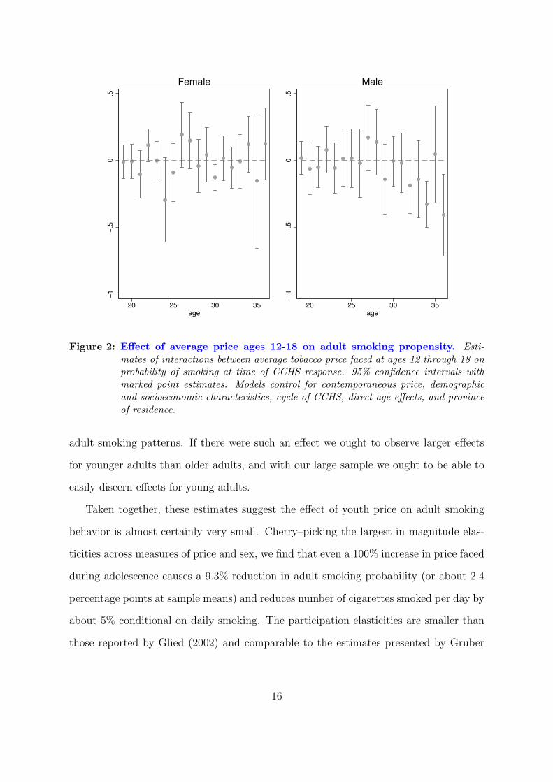
−1

−.5

0.5

20 25 30 35age

Female

−1

−.5

0.5

20 25 30 35age

Male

Figure 2: Effect of average price ages 12-18 on adult smoking propensity. Esti-mates of interactions between average tobacco price faced at ages 12 through 18 onprobability of smoking at time of CCHS response. 95% confidence intervals withmarked point estimates. Models control for contemporaneous price, demographicand socioeconomic characteristics, cycle of CCHS, direct age effects, and provinceof residence.

adult smoking patterns. If there were such an effect we ought to observe larger effects

for younger adults than older adults, and with our large sample we ought to be able to

easily discern effects for young adults.

Taken together, these estimates suggest the effect of youth price on adult smoking

behavior is almost certainly very small. Cherry–picking the largest in magnitude elas-

ticities across measures of price and sex, we find that even a 100% increase in price faced

during adolescence causes a 9.3% reduction in adult smoking probability (or about 2.4

percentage points at sample means) and reduces number of cigarettes smoked per day by

about 5% conditional on daily smoking. The participation elasticities are smaller than

those reported by Glied (2002) and comparable to the estimates presented by Gruber

16

and Zinman (2001) for pregnant women. Unlike Glied, we do not find that men exhibit

higher intertemporal elasticities than women, indeed, our estimates weakly suggest the

opposite.4 However, the comparison is difficult due to differences in samples, ages, and

price measures.

As a final piece of evidence, in Table 4 we report results of a multinomial logit

regression of smoker type on youth and current prices and personal characteristics. We

reason as follows: we have shown that youth prices affect youth smoking behavior,

increasing age of initiation and reducing probability of youth initiation. If initiation is

detered, we should find that adults who, all else equal, faced higher youth prices are

more likely to be never smokers than current or former smokers. If initiation is deferred

but not deterred, we should find that adults who faced higher youth prices are no more

likely to be never smokers than current or former smokers. For example, recall that the

estimates in the last two columns of table 2, bottom row, suggest that a 10% increase

in youth prices reduce probability of initiation by age 18 by three to four percent. If

youths induced not to initiate by age 18 initiate thereafter, so smoking is deferred but

not deterred, we will observe them as current or former smokers, but if they never initiate

we will observe them later in life as never–smokers.

Multinomial logit results are reported in Table 4. When we use price at age 14 as

our measure of youth price we find no statistically or economically significant effects on

smoker type. Average price over ages 14 through 16 modestly increases probability of

never smoker, albeit not statistically significantly, and statistically significantly reduces

probability of current smoking for women. A 10% increase in youth prices reduces

probability of current smoking for women by slightly less than one percent and increases

probability of never smoking by about half of one percent. The results for prices over

ages 12 through 18 are similar, and the probability of never smoking is statistically

4Stehr (2007) studies sex differences in smoking elasticies in detail and finds that women are roughlytwice as responsive as men.

17

Women

Men

.2.2

5.3

.35

Sm

okin

g p

rop

en

sity

20 25 30 35 40age

Figure 3: Simulation results. Actual smoking propensities by age predicted from multi-variate model (solid lines) and counterfactual smoking propensities predicted un-der counterfactual prices (dashed lines). Counterfactual prices hold prices in eachprovince at their 1990 levels through the end of 1994, simulating a world in whichthe 1991 to 1994 increase apparent in Figure 1 did not occur.

significant for women. These estimates are weak evidence of a long–term effect of youth

prices on smoking status later in life. Roughly, the estimates suggest that doubling the

price faced by youth would decrease the probability of current smoking later in life by

10% (or about 2.5 percentage points) and increase the probability of never smoking by

about 7.5% (or about 1.75 percentage points).

4.3 Numerical simulation of counterfactual tax policy.

We have found mixed evidence that cigarette price in youth is a weak determinant of

smoking behavior in adulthood; our largest estimates of the elasticity of adult smoking

to youth prices are around 0.1. To illustrate the magnitude of the long term effects,

18

we simulated the proportion of daily smokers using actual and counterfactual cigarette

prices. Following Auld (2005), we consider the counterfactual case in which the Federal

government did not impose high taxes during 1991 through 1994. We simulate the

proportion of smokers using the estimates of equation (4), assigning cigarette prices in

1991 to 1994 using 1990 levels. The results are illustrated in top panel of Figure 3,

which displays the difference in the proportion of the smokers for both sexes using the

actual and the counterfactual cigarette prices. The figure illustrates the difference in the

proportion of daily smokers at ages 21 to 29 for respondents who faced the actual and the

counterfactual cigarette prices in youth. Counterfactual adult smoking probabilities are

very similar to actual smoking probabilities, although observe that the model predicts a

slight counterfactual increase in smoking propensity. These results are consistent with

those of Auld (2005).

5 Conclusions.

Exploiting large and plausibly exogenous changes in tobacco tax rates in Canada in

the early 1990s and large repeated cross–sections, we present evidence on the effects of

changes in cigarette prices on smoking during youth and early adulthood. We find that

adults in 2001 through 2005 who faced particularly high prices during adolescence due

to a transient Federal tobacco tax between 1991 and 1994 were less likely to initiate into

daily smoking and, conditional on smoking daily, smoke slightly less than observationally

equivalent adults who faced lower prices during peak adolescent initiation years. Higher

youth prices are also associated with slightly higher probability of adults reporting that

they do not and never have smoked, consistent with a small deterrence effect.

However, we find that these effects are qualitatively very small, and the evidence

is mixed. Even with a sample of almost 100,000 individuals price faced during adoles-

cence is often statistically insignificant, and even the largest point estimates suggest the

19

magnitude of the effect is small. The estimates are sensitive to how we measure price

faced during adolescence: previous related research uses price at age 14, but we find

that averaging prices over longer age intervals, such as 14 through 16 or 12 through 18,

tends to yield larger and more precisely measured estimates. Even picking the largest

estimates across sexes, measures of price, measures of smoking propensity and intensity,

and empirical strategies yields estimates of the elasticity of adult smoking to youth price

on the order of 0.1. That is, a 10% increase in youth price leads to at most roughly a 1%

decrease in smoking later in life. Further, we find no clear pattern over age: adults in

their early twenties respond to changes in youth price about the same as those in their

late thirties.

Our analysis has several important limitations. Perhaps of most concern is our

reconstruction of past behavior from retrospective questions. We do not observe time–

varying covariates during adolescence, notably, we do not observe province of residence,

and hence tobacco price, during adolescence and must assume the respondent has not

moved across provinces. Further, retrospective data may be subject to other measure-

ment error, and that error may be more of a problem for older respondents in our sample.

We present simulation evidence suggesting that cross-province moves induce very mod-

est attenuation bias, and our estimates of the effects of adolescent price on adolescent

smoking patterns are consistent with recent estimates which do not rely on retrospective

information, so we believe that our measurement issues are unlikely to be driving the

results. Nonetheless, our estimates of the effect of youth price on adult smoking are

likely to be biased towards zero, so our results should be interpreted with that caveat in

mind.

We conclude that changes in youth smoking patterns induced by tobacco taxation

likely carry over, through addiction, to adult smoking patterns, but that this effect is

qualitatively small.

20

Appendix.

As discussed in section (2.3), we do not observe province of residence during youth and

must assume that the respondent has not moved across provinces when assigning past

prices. Here, we report on a small Monte Carlo experiment constructed to investigate

the magnitude of the resulting attenuation bias in a sampling environment similar to

our data.

To mimic the broad features of the data, we set the number of observations per

replication to n=90,000. In each of 30 province–cycle (10 provinces and three cycles)

cells we assigned a price pij which ranges from -0.25 to 0.072 in steps of 0.024. These

numbers were chosen to yield a mean price of 0.6 and an unconditional price standard

deviation of 0.2, matching the moments of the data (Table 1). The data generating

process was,

yij = −0.1pij + uij, (6)

where i indexes simulated observations, pij is the price assigned in province–cycle j, and

uij ∼ N(0, 1). To simulate unobserved moves across provinces, we construct observed

price, perrorij , which equals pij with probability 0.9 and with probability 0.1 is set to the

price from a randomly drawn province–cycle. We simulated R=10,000 replications from

this process.

In table 5 we report selected statistics from the simulations. Estimates using mismea-

sured prices, βerror, are attenuated by about 10% relative to (unbiased and consistent)

estimates using actual prices (βtrue). Standard errors are not biased by mismeasurement.

t–ratios against the false null that the true coefficient is zero, denoted ttrue and terror

are, therefore, centered on lower values when we use data subject to measurement error,

and tests of the null that the coefficient is equal to zero have diminished power.

We conclude from this exercise that, in our case, measurement error resulting from

not observing province of residence during adolescence is not trivial but neither is it

21

serious. Our point estimates are attenuated by about 10%, with a resulting small loss

in power.

References

Angrist, J. and J. Pischke, Mostly Harmless Econometrics: An Empiricist’s Com-panion, Princeton University Press, 2009.

Aristei, D. and L. Pieroni, “Addiction, social interactions, and gender differences incigarette consumption,” Empirica, 2009. Forthcoming.

Auld, M. C., “Causal effect of early initiation on adolescent smoking patterns,” Cana-dian Journal of Economics, 2005, 38 (3), 709–34.

Becker, G. and K. Murphy, “A theory of rational addiction,” Journal of PoliticalEconomy, 1988, 96, 675–700.

Cameron, A.C. and P.K. Trivedi, Microeconometrics: Methods and applications,Cambridge University Press, 2005.

Carpenter, C. and P.J. Cook, “Cigarette taxes and youth smoking: New evidencefrom national, state, and local Youth Risk Behavior Surveys,” Journal of Health Eco-nomics, 2008, 27 (2), 287–299.

Cawley, J., S. Markowitz, and J. Tauras, “Lighting Up and Slimming Down:The Effects of Body Weight and Cigarette Prices on Adolescent Smoking Initiation,”Journal of Health Economics, 2004, 23 (2), 293–311.

DeCicca, P., D. Kenkel, and A. Mathios, “Cigarette taxes and the transition fromyouth to adult smoking: Smoking initiation, cessation, and participation,” Journal ofHealth Economics, 2008, 27 (4), 904–917.

Eisenberg, D. and B. Rowe, “The effect of smoking in young adulthood on smokinglater in life: Evidence based on the Vietnam Era draft lottery,” Forum for HealthEconomics and Policy, 2009, 12 (2), 1–32.

Gilleskie, D. and K. Strumpf, “The behavioral dynamics of youth smoking,” Journalof Human Resources, 2005, 40 (4), 822–66.

Glied, S., “Youth tobacco control: Reconciling theory and empirical evidence,” Journalof Health Economics, 2002, 21, 117–135.

, “Is smoking delayed smoking averted?,” American Journal of Public Health, 2003,93 (3), 412–416.

Gruber, J. and J. Zinman, “Youth smoking in the U.S.: Evidence and implications,”in J. Gruber, ed., Risky behaviors among youths, University of Chicago Press, 2001.

22

Hamilton, V., C. Levinton, Y. St-Pierre, and F. Grimard, “The effect of tobaccotax cuts on cigarette smoking in Canada,” Canadian Medical Association Journal,1997, 156 (2), 187–91.

Harris, J. and S. Chan, “The continuum of addiction: cigarette smoking in relationto price among Americans aged 15-29,” Health Economics, 1999, 8, 81–6.

Jones, A., “A double–hurdle model of cigarette consumption,” Journal of AppliedEconometrics, 1989, 4 (1), 23–39.

Kenkel, D., D. Lillard, and A. Mathios, “Accounting for misclassification error inretrospective smoking data,” Health Economics, 2004, 13 (10), 1031–44.

Lewitt, E. and M. Grossman, “The effects of government regulation on teenagesmoking,” Journal of Law and Economics, 1981, 24, 545–573.

Paul, S., L. Blizzard, G. Patton, T. Dwyer, and A. Venn, “Parental smokingand smoking experimentation in childhood increase the risk of being a smoker 20 yearslater: the Childhood Determinants of Adult Health Study,” Addiction, 2009, 103 (5),846–853.

Sen, A. and T. Wirjanto, “Estimating the impacts of cigarette taxes on youth smok-ing participation, initiation, and persistence: empirical evidence from Canada,” Healtheconomics, 2009.

Stehr, M., “The effect of cigarette taxes on smoking among men and women,” HealthEconomics, 2007, 16 (12), 1333–1344.

Studlar, D., Tobacco control: Comparative politics in the United States and Canada,Broadview Press, 2002.

Tauras, J. and F. Chaloupka, “Price, Clean Indoor Air, and Cigarette Smoking:Evidence from the Longitudinal Data for Young Adults,” Technical Report 6937,National Bureau of Economic Research 1999.

Warner, K., F. Chaloupka, P. Cook, W. Manning, J. Newhouse, T. Novotny,T. Schelling, and J. Townsend, “Criteria for Determining an Optimal CigaretteTax: The Economist’s Perspective,” Tobacco Control, 1995, 4, 380–86.

23

Table 1: Summary statistics.

Population Female Male

mean s.d. mean s.d. mean s.d.

Age smoked first whole cigarette 15.11 3.23 14.93 3.06 15.31 3.39Age started smoking daily 16.67 3.26 16.41 3.19 16.98 3.32Daily smoker 0.25 0.43 0.24 0.42 0.27 0.45Occasional smoker 0.07 0.26 0.07 0.26 0.08 0.27Cigarettes per day† 14.84 7.70 13.35 7.02 16.33 8.11Current smoker 0.33 0.47 0.31 0.46 0.35 0.48Former smoker 0.33 0.47 0.34 0.47 0.32 0.47Never smoker 0.34 0.47 0.35 0.48 0.33 0.47

Current cigarette price 1.05 0.21 1.05 0.21 1.06 0.21Cigarette price at age 14 0.59 0.21 0.60 0.22 0.59 0.21Cigarette price at age 14-16 0.62 0.20 0.62 0.20 0.61 0.20Cigarette price at age 12-18 0.66 0.17 0.66 0.16 0.65 0.17

Less than high school 0.11 0.31 0.09 0.29 0.12 0.33High school 0.19 0.39 0.18 0.38 0.21 0.41Post secondary 0.11 0.32 0.11 0.32 0.11 0.31University 0.59 0.49 0.62 0.49 0.56 0.50

No household income 0.01 0.06 0.01 0.06 0.01 0.07Income < 5000 0.01 0.11 0.01 0.12 0.01 0.10Income 5,000- 9,999 0.03 0.17 0.04 0.19 0.02 0.15Income 10,000-14,999 0.05 0.21 0.06 0.24 0.03 0.18Income 15,000-19,999 0.06 0.24 0.07 0.26 0.05 0.22Income 20,000-29,999 0.11 0.31 0.11 0.31 0.10 0.30Income 30,000-39,999 0.12 0.32 0.12 0.33 0.12 0.32Income 40,000-49,999 0.11 0.32 0.11 0.31 0.12 0.32Income 50,000-59,999 0.14 0.34 0.13 0.34 0.14 0.35Income 60,000-79,999 0.16 0.36 0.15 0.34 0.24 0.43Income > 80,000 0.21 0.41 0.19 0.39 0.24 0.43

Household size 2.89 1.36 2.97 1.34 2.79 1.38Immigrant 0.10 0.30 0.10 0.30 0.10 0.30Married 0.54 0.5 0.57 0.5 0.51 0.50Pregnant - - 0.06 0.23 - -Depression (scaled 0 to 8) 0.65 1.85 0.81 2.05 0.47 1.58Age 29.42 5.77 29.38 5.69 29.49 5.85

Observations 95,408 50,684 44,313

Notes. Other variables included in the estimated models but not reported here include:dummies indicating ethnicity, province of residence, cycle of the data, and age of respon-dents. †Cigarettes per day calculated over daily smokers only.

24

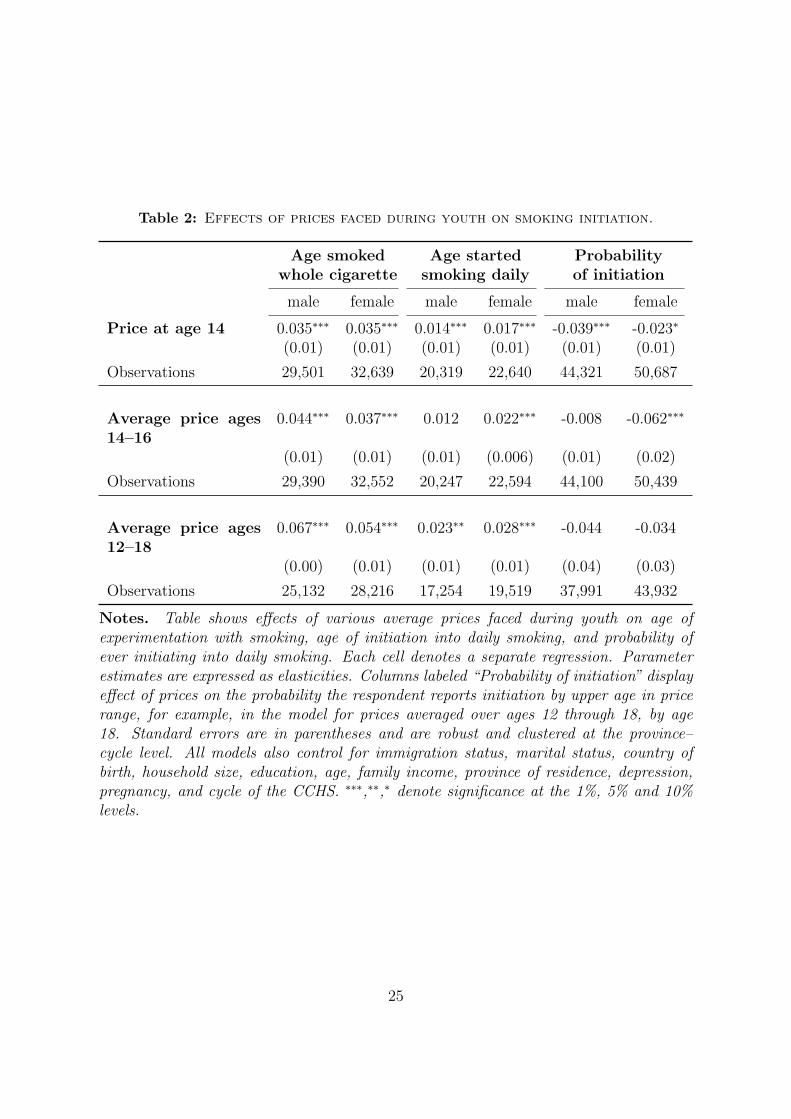
Table 2: Effects of prices faced during youth on smoking initiation.

Age smoked Age started Probabilitywhole cigarette smoking daily of initiation

male female male female male female

Price at age 14 0.035∗∗∗ 0.035∗∗∗ 0.014∗∗∗ 0.017∗∗∗ -0.039∗∗∗ -0.023∗

(0.01) (0.01) (0.01) (0.01) (0.01) (0.01)

Observations 29,501 32,639 20,319 22,640 44,321 50,687

Average price ages14–16

0.044∗∗∗ 0.037∗∗∗ 0.012 0.022∗∗∗ -0.008 -0.062∗∗∗

(0.01) (0.01) (0.01) (0.006) (0.01) (0.02)

Observations 29,390 32,552 20,247 22,594 44,100 50,439

Average price ages12–18

0.067∗∗∗ 0.054∗∗∗ 0.023∗∗ 0.028∗∗∗ -0.044 -0.034

(0.00) (0.01) (0.01) (0.01) (0.04) (0.03)

Observations 25,132 28,216 17,254 19,519 37,991 43,932

Notes. Table shows effects of various average prices faced during youth on age ofexperimentation with smoking, age of initiation into daily smoking, and probability ofever initiating into daily smoking. Each cell denotes a separate regression. Parameterestimates are expressed as elasticities. Columns labeled “Probability of initiation” displayeffect of prices on the probability the respondent reports initiation by upper age in pricerange, for example, in the model for prices averaged over ages 12 through 18, by age18. Standard errors are in parentheses and are robust and clustered at the province–cycle level. All models also control for immigration status, marital status, country ofbirth, household size, education, age, family income, province of residence, depression,pregnancy, and cycle of the CCHS. ∗∗∗,∗∗,∗ denote significance at the 1%, 5% and 10%levels.

25

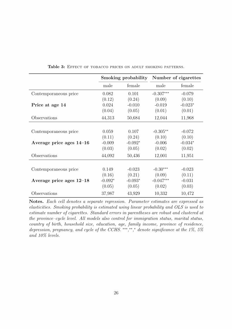
Table 3: Effect of tobacco prices on adult smoking patterns.

Smoking probability Number of cigarettes

male female male female

Contemporaneous price 0.082 0.101 -0.307∗∗∗ -0.079(0.12) (0.24) (0.09) (0.10)

Price at age 14 0.024 -0.010 -0.019 -0.023∗

(0.04) (0.05) (0.01) (0.01)

Observations 44,313 50,684 12,044 11,968

Contemporaneous price 0.059 0.107 -0.305∗∗ -0.072(0.11) (0.24) (0.10) (0.10)

Average price ages 14–16 -0.009 -0.092∗ -0.006 -0.034∗

(0.03) (0.05) (0.02) (0.02)

Observations 44,092 50,436 12,001 11,951

Contemporaneous price 0.149 -0.023 -0.30∗∗∗ -0.023(0.16) (0.21) (0.09) (0.11)

Average price ages 12–18 -0.092∗ -0.093∗ -0.047∗∗∗ -0.031(0.05) (0.05) (0.02) (0.03)

Observations 37,987 43,929 10,332 10,472

Notes. Each cell denotes a separate regression. Parameter estimates are expressed aselasticities. Smoking probability is estimated using linear probability and OLS is used toestimate number of cigarettes. Standard errors in parentheses are robust and clustered atthe province–cycle level. All models also control for immigration status, marital status,country of birth, household size, education, age, family income, province of residence,depression, pregnancy, and cycle of the CCHS. ∗∗∗,∗∗,∗ denote significance at the 1%, 5%and 10% levels.

26

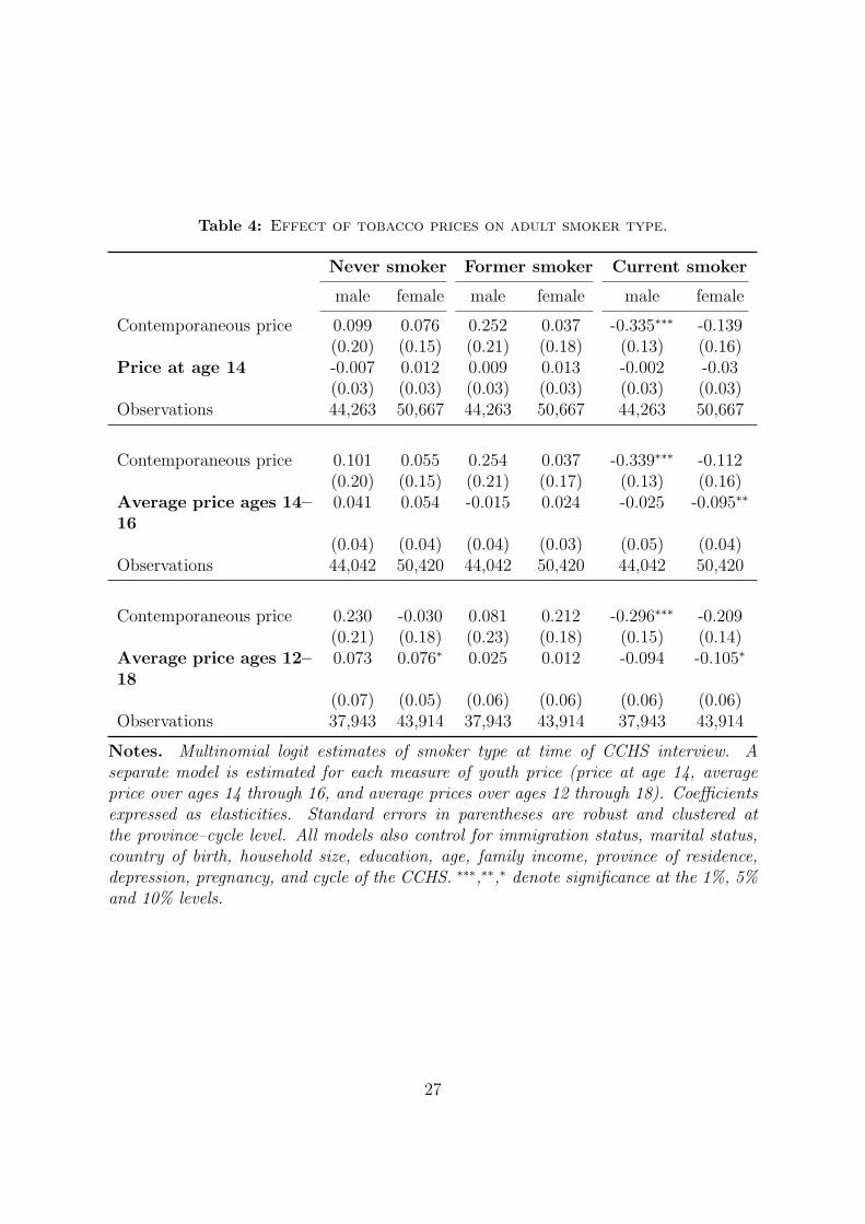
Table 4: Effect of tobacco prices on adult smoker type.

Never smoker Former smoker Current smoker

male female male female male female

Contemporaneous price 0.099 0.076 0.252 0.037 -0.335∗∗∗ -0.139(0.20) (0.15) (0.21) (0.18) (0.13) (0.16)

Price at age 14 -0.007 0.012 0.009 0.013 -0.002 -0.03(0.03) (0.03) (0.03) (0.03) (0.03) (0.03)

Observations 44,263 50,667 44,263 50,667 44,263 50,667

Contemporaneous price 0.101 0.055 0.254 0.037 -0.339∗∗∗ -0.112(0.20) (0.15) (0.21) (0.17) (0.13) (0.16)

Average price ages 14–16

0.041 0.054 -0.015 0.024 -0.025 -0.095∗∗

(0.04) (0.04) (0.04) (0.03) (0.05) (0.04)Observations 44,042 50,420 44,042 50,420 44,042 50,420

Contemporaneous price 0.230 -0.030 0.081 0.212 -0.296∗∗∗ -0.209(0.21) (0.18) (0.23) (0.18) (0.15) (0.14)

Average price ages 12–18

0.073 0.076∗ 0.025 0.012 -0.094 -0.105∗

(0.07) (0.05) (0.06) (0.06) (0.06) (0.06)Observations 37,943 43,914 37,943 43,914 37,943 43,914

Notes. Multinomial logit estimates of smoker type at time of CCHS interview. Aseparate model is estimated for each measure of youth price (price at age 14, averageprice over ages 14 through 16, and average prices over ages 12 through 18). Coefficientsexpressed as elasticities. Standard errors in parentheses are robust and clustered atthe province–cycle level. All models also control for immigration status, marital status,country of birth, household size, education, age, family income, province of residence,depression, pregnancy, and cycle of the CCHS. ∗∗∗,∗∗,∗ denote significance at the 1%, 5%and 10% levels.

27

Table 5: Monte Carlo results.

mean s.d. s.e.

Coefficient estimates (true: β = −0.100):

βtrue -0.099 0.016 0.016

βerror -0.090 0.016 0.016

βerror

/βtrue 0.900 0.073

t-ratios against false null β = 0:ttrue -6.222 1.000terror -5.598 1.000

Notes. 90,000 observations in each of 10,000 replications. Estimates from model withtrue prices are denoted with a subscript “true” and models with simulated measurementerror arising from cross–province moves are denoted with a subscript “error.” s.d. de-notes observed standard deviation and s.e. estimated standard errors.

28

contributions to the empirical analysis of addictive behaviors · contributions to the empirical...

Documents