contributions to the control of hybrid and swithced linear ... · contributions to the control of...
TRANSCRIPT
Contributions to the Control of Hybrid and
Switched Linear Systems
vorgelegt vonM.Sc. Yashar Kouhi Anbarangeboren in Bandaranzali, Iran
von der Fakultat IV -Elektrotechnik und Informatikder Technischen Universitat Berlin
zur Erlangung des akademischen Grades
Doktor der Ingenieurwissenschaften- Dr.-Ing. -
genehmigte Dissertation
Promotionsausschuss:
Vorsitzender: Prof. Dr.-Ing. Clemens GuhmannGutachter: Prof. Dr.-Ing. Jorg RaischGutachter: Prof. Robert ShortenGutachter: Dr. Paul Curran
Tag der wissenschaftlichen Aussprache: 31. Oktober 2014
Berlin 2014D 83

i
Abstract
Hybrid linear systems are a class of hybrid systems where the continuous time evolu-tion is governed by a set of first order linear ordinary differential equations and the jumpdynamics are described by a set of first order linear difference equations. Switched linearsystems are a subclass of hybrid linear systems with a continuous evolution of the systemstates. Due to the large number of physical applications, control of hybrid and switchedlinear systems has received considerable attention over the past years. This dissertationprovides novel contributions to the control of such systems and extends some existingresults in this area. This work focuses on different problems regarding stability andstabilization of switched linear systems and optimal control of hybrid linear systems.
The major part of this thesis concerns stability and stabilization of switched linearsystems. The results are primarily presented in terms of conditions for stability ofautonomous switched systems. Then, stabilization methods aim at designing a localstate feedback for each mode of a controlled switched system to satisfy the stabilitycriteria for the closed loop system modes. Parts of these results rely on the conceptof common left eigenvectors and left eigenstructure assignment. To this end, severaltechniques for eigenstructure assignment in the context of linear systems are developed.Afterwards, these techniques are employed for characterizing exponential stability andfor stabilization of a class of switched linear systems with state dependent switching andcertain restrictions on the switching manifolds. In addition, they are used for quadraticstabilization of a class of controlled switched linear systems with arbitrary switchingsignals where the open loop constituent matrices share an invariant subspace to whicha common quadratic Lyapunov function can be associated. Another stability approachmakes use of the Kalman-Yakubovic-Popov lemma to demonstrate quadratic stabilityof a class of switched linear systems. This class is characterized by arbitrary switchingbetween two modes, where the difference of the constitute matrices is of rank m ≥ 1, andto which a symmetric transfer function matrix can be associated. These results extendexisting results in quadratic stability of rank-1 difference switched linear systems.
The thesis also addresses problems in linear quadratic control of hybrid linear systems.In these problems, cost functions are quadratic, the final time and the number andsequence of switches are given. Constraints are specified by linear (in-)equalities in thestate space. Switching between different dynamics may either occur at fixed or freetime instances. A parameterization method with respect to initial and end points ofeach interval in a generalized time domain is employed. Numerical solutions for suchproblems are suggested.

ii
iii
Zusammenfassung
Hybride lineare Systeme sind eine Klasse von hybriden Systemen, bei denen die kontinu-ierliche Zeitentwicklung durch einen Satz von linearen Differentialgleichungen erster Ordnung,und die Sprungdynamik durch einen Satz von linearen Differenzengleichungen erster Ordnungbeschrieben werden. Geschaltete lineare Systeme sind eine Unterklasse von hybriden linea-ren Systemen mit einer stetigen Zeitentwicklung der Systemzustande. Aufgrund der großenAnzahl physikalischer Anwendungen erfuhr die Regelung von hybriden und geschalteten linea-ren Systemen in den letzten Jahren betrachtliche Aufmerksamkeit. Diese Dissertation stelltneue Beitrage zur Regelung solcher Systeme vor und erweitert einige vorhandene Ergebnissein diesem Bereich. Diese Arbeit konzentriert sich auf verschiedene Aspekte der Stabilitat undStabilisierung geschalteter linearer Systeme sowie der optimalen Regelung hybrider linearerSysteme.
Der großte Teil dieser Arbeit betrifft die Stabilitat und Stabilisierung von geschalteten li-nearen Systemen. Die Darstellung der Ergebnisse bezieht sich in erster Linie auf Bedingungenfur die Stabilitat autonomer geschalteter linearer Systeme. Stabilisierungsverfahren zielen dannauf den Entwurf einer lokalen Zustandsruckfuhrung fur jeden Modus eines geregelten geschal-teten linearen Systems, um die Stabilitatskriterien fur die Modi des geschlossenen Regelkreiseszu befriedigen. Teile dieser Ergebnisse beruhen auf dem Konzept gemeinsamer linker Eigen-vektoren und der Zuweisung linker Eigenstruktur. Zu diesem Zweck werden mehrere Verfahrenzur Zuweisung der Eigenstruktur von linearen Systemen entwickelt. Anschließend werden dieseTechniken zur Charakterisierung exponentieller Stabilitat und zur Stabilisierung einer Klassevon geschalteten linearen Systemen mit zustandsabhangigem Schalten unter bestimmten Ein-schrankungen bezuglich der Schaltmannigfaltigkeiten eingesetzt. Daruber hinaus werden siezur quadratischen Stabilisierung einer Klasse von beliebig schaltenden linearen Systemen ein-gesetzt, in der die Dynamikmatrizen des offenen Kreises einen invarianten Untervektorraumgemeinsam haben, der mit einer gemeinsamen quadratischen Lyapunov-Funktion assoziiertwerden kann. Ein weiterer Stabilitatsansatz nutzt das Kalman-Yakubovic-Popov-Lemma, umquadratische Stabilitat einer Klasse von geschalteten linearen Systemen zu zeigen. Diese Klas-se wird von beliebigem Schalten zwischen zwei Modi gekennzeichnet, fur welche die Differenzder Dynamikmatrizen von Rang m ≥ 1 ist, und mit denen eine symmetrische Ubertragungs-funktionsmatrix assoziiert werden kann. Diese Ergebnisse erweitern vorhandene Ergebnisse zurquadratischen Stabilitat geschalteter linearer Systeme, bei denen die Differenz der Dynamik-matrizen Rang 1 aufweist.
Die Dissertation befasst sich auch mit der linear quadratischen Regelung von hybridenlinearen Systemen. Hierbei sind die Kostenfunktionen quadratisch, der Zeithorizont und dieAnzahl und Reihenfolge des Schaltens gegeben. Einschrankungen sind durch lineare (Un-)Gleichungen im Zustandsraum gegeben. Die Zeitpunkte des Schaltens zwischen unterschiedli-chen Dynamiken konnen entweder vorgegeben oder frei sein. Ein Parametrierungsverfahren inBezug auf Ausgangs- und Endpunkte der einzelnen Intervalle eines generalisierten Zeitbereichswird verwendet. Numerische Losungen werden fur solche Aufgaben vorgeschlagen.

iv

v
Acknowledgements
I would like to gratefully acknowledge my supervisor, Prof. Dr-.Ing. Jorg Raisch, forgiving me the opportunity to be a Ph.D. student in the Control Systems Group atTechnische Universitat (TU) Berlin and to be a member of his group at the Max PlanckInstitute (MPI) for Dynamics of Complex Technical Systems in Magdeburg. Havinghis support and encouragement, I could attend in several summer school courses andscientific conferences during my Ph.D. program, and thereby grow as a better researcher.His guidance, advice, and careful review has also tremendously enhanced the quality ofthis thesis. My thank extends to Prof. Robert Shorten at IBM Research Ireland, one ofthe greatest scientists I have ever met. He introduced me one of his research projects,offered the key idea, and willingly supported me to develop the results of their team. Iam very pleased to acknowledge Prof. Ricardo G. Sanfelice at the University of Arizona.Being a participant in his lectures at HYCON-EECI 2011 in Paris, I got familiar withmany fundamental concepts in the control of hybrid systems, and in a conversationwith him I found a new direction of research in this field. I greatly benefited fromhis extensive knowledge afterwards via phone discussions and receiving comments byEmails. Prof. Shorten and Prof. Sanfelice have truly made huge impacts on my researchcareer in a short period of time. I would like also to express my thanks to the member ofPh.D. exam committee, Dr. Paul Curran from University College Dublin, for acceptingthe evaluation of this thesis. His brilliant suggestions and insightful criticism havesignificantly improved the quality of this work.
I am grateful for getting to know the nice former colleagues at TU Berlin. Inparticular, I would like to thank Dipl.-Ing. Steffen Hofmann for assisting me with hisincredible computer skills, M.Sc. Truong Duc Trung, and Dipl.-Ing. Behrang MonajemiNejad for creating enjoyable moments for me. I appreciate to express my thanks andgratitude to Mrs. Janine Holzmann, the secretary of the group at the MPI Magdeburg.She is very kind, and sincerely helps the other people.
Finally, I would like to mention my parents, Golagha and Tahere, who have beenspiritually supporting me in the entire life. Also, my family members in Germany, mysister, Yalda, her husband, Farough, and my uncle, Bijan, helped me considerably. Withtheir support I never felt alone in my hardships during the doctoral studies.

vi

vii
Publications
Some ideas and figures have appeared previously in the following publications:
• Y. Kouhi, N. Bajcinca, J. Raisch, and R. Shorten. On the quadratic stabilityof switched linear systems associated with symmetric transfer function matrices.Automatica, 50(11):2872–2879, 2014
• N. Bajcinca, D. Flockerzi, and Y. Kouhi. On a geometrical approach to quadraticLyapunov stability and robustness. In Proc. of the 52th Conference on Decisionand Control, pages 1–6, 2013
• Y. Kouhi, N. Bajcinca, J. Raisch, and R. Shorten. A new stability result forswitched linear systems. In Proc. of the European Control Conference, pages 2152–2156, 2013a
• Y. Kouhi, N. Bajcinca, and R. G. Sanfelice. Suboptimality bounds for linearquadratic problems in hybrid linear systems. In Proc. of the European ControlConference, pages 2663–2668, 2013b
• Y. Kouhi and N. Bajcinca. On the left eigenstructure assignment and state feedbackdesign. In Proc. of the American Control Conference, pages 4326–4327, 2011a
• Y. Kouhi and N. Bajcinca. Nonsmooth control design for stabilizing switched linearsystems by left eigenstructure assignment. In Proc. of the IFAC World Congress,pages 380–385, 2011b
• Y. Kouhi and N. Bajcinca. Robust control of switched linear systems. In Proc. ofthe 50th IEEE Conference on Decision and Control and European Control Confer-ence, pages 4735–4740, 2011c

viii
CONTENTS ix
Contents
Abstract i
Zusammenfassung iii
Acknowledgements v
Publications vii
Contents ix
List of Figures xiii
1 Introduction and literature review 1
1.1 Hybrid and switched linear systems . . . . . . . . . . . . . . . . . . . . . 1
1.2 Model of hybrid and switched linear systems . . . . . . . . . . . . . . . 7
1.3 Stability of switched linear systems . . . . . . . . . . . . . . . . . . . . . 9
1.3.1 Common Quadratic Lyapunov function (CQLF) . . . . . . . . . . 9
1.4 Stabilization of switched linear systems . . . . . . . . . . . . . . . . . . . 11
1.5 Optimal control of hybrid linear systems . . . . . . . . . . . . . . . . . . 12
1.6 Organization of the thesis . . . . . . . . . . . . . . . . . . . . . . . . . . 13
2 Left eigenstructure assignment 15
2.1 Introduction . . . . . . . . . . . . . . . . . . . . . . . . . . . . . . . . . . 15
2.2 Left eigenvector assignment . . . . . . . . . . . . . . . . . . . . . . . . . 15
2.2.1 Single-input systems . . . . . . . . . . . . . . . . . . . . . . . . . 16
2.2.1.1 Closed loop stability . . . . . . . . . . . . . . . . . . . . 18
2.2.1.2 Pole placement . . . . . . . . . . . . . . . . . . . . . . . 19
2.2.1.3 Single shift eigenvalue . . . . . . . . . . . . . . . . . . . 20
2.2.1.4 Partial pole placement . . . . . . . . . . . . . . . . . . . 20
2.2.2 Multi-input systems . . . . . . . . . . . . . . . . . . . . . . . . . 21
2.2.2.1 Closed loop stability having (n− 1) inputs . . . . . . . . 23
2.3 Left eigenstructure assignment . . . . . . . . . . . . . . . . . . . . . . . . 25
2.4 Conclusions . . . . . . . . . . . . . . . . . . . . . . . . . . . . . . . . . . 28

x CONTENTS
3 Switched linear systems with state dependent switching 29
3.1 Introduction . . . . . . . . . . . . . . . . . . . . . . . . . . . . . . . . . . 29
3.2 Exponential stability of switched linear systems . . . . . . . . . . . . . . 30
3.3 Exponential stabilization of controlled switched systems . . . . . . . . . . 35
3.3.1 Stabilization of single-input controlled switched systems . . . . . . 35
3.3.2 Stabilization of multi-input controlled switched systems . . . . . . 40
3.4 Conclusions . . . . . . . . . . . . . . . . . . . . . . . . . . . . . . . . . . 42
4 Switched linear systems with arbitrary switching signals 43
4.1 Introduction . . . . . . . . . . . . . . . . . . . . . . . . . . . . . . . . . . 43
4.2 Quadratic stability of switched linear systems . . . . . . . . . . . . . . . 44
4.2.1 Stability of switched systems with a common invariant subspace . 47
4.2.1.1 Stability with (n− 1) common right eigenvectors . . . . 48
4.2.1.2 Stability with (n− 1) common real left eigenvectors . . . 49
4.3 Robust Stability of switched linear systems . . . . . . . . . . . . . . . . . 53
4.3.1 Robust stability with (n− 1) common real left eigenvectors . . . . 54
4.4 Quadratic stabilization of switched linear systems . . . . . . . . . . . . . 56
4.4.1 Block similar controlled switched linear systems . . . . . . . . . . 57
4.4.2 Stabilization and common invariant subspaces . . . . . . . . . . . 58
4.4.2.1 Stabilization for the case of (n− 1) dimensional commoninvariant subspace . . . . . . . . . . . . . . . . . . . . . 61
4.4.2.2 Stabilization based on (n−1) common real left eigenvectors 61
4.4.3 Stabilization and perturbed invariant subspaces . . . . . . . . . . 64
4.5 Robust control design with (n− 1) control inputs . . . . . . . . . . . . . 69
4.6 Conclusions . . . . . . . . . . . . . . . . . . . . . . . . . . . . . . . . . . 70
5 Rank-m difference switched systems 71
5.1 Introduction . . . . . . . . . . . . . . . . . . . . . . . . . . . . . . . . . . 71
5.2 Symmetric transfer function matrices . . . . . . . . . . . . . . . . . . . . 72
5.3 Strictly Positive Real systems (SPR) . . . . . . . . . . . . . . . . . . . . 78
5.3.1 Symmetric SPR systems with nonsingular D . . . . . . . . . . . . 78
5.3.2 Symmetric SPR systems with singular D . . . . . . . . . . . . . . 80
5.4 Stability of a class of switched linear systems . . . . . . . . . . . . . . . 82
5.4.1 Quadratic stability . . . . . . . . . . . . . . . . . . . . . . . . . . 82
5.4.2 Weak quadratic stability . . . . . . . . . . . . . . . . . . . . . . . 86
5.5 Stabilization of controlled switched linear systems . . . . . . . . . . . . . 93
5.6 Conclusions . . . . . . . . . . . . . . . . . . . . . . . . . . . . . . . . . . 95
6 Control of hybrid linear systems 97
6.1 Introduction . . . . . . . . . . . . . . . . . . . . . . . . . . . . . . . . . . 97
6.2 Stability of a class of hybrid linear systems . . . . . . . . . . . . . . . . . 98

CONTENTS xi
6.3 Robust Stability of hybrid linear systems . . . . . . . . . . . . . . . . . . 101
6.4 LQR design for a class of hybrid linear systems (Scenario I) . . . . . . . 105
6.4.1 Suboptimal solutions to flow equations . . . . . . . . . . . . . . . 109
6.4.2 Suboptimal solutions for jumps . . . . . . . . . . . . . . . . . . . 112
6.4.3 Constrained QP problems for the hybrid linear system . . . . . . 116
6.4.3.1 Lower bound for optimal control problem . . . . . . . . 117
6.4.3.2 Algorithm to compute solution and an upper bound . . 118
6.5 LQR design for a class of hybrid linear systems (Scenario II) . . . . . . . 124
6.5.1 Optimal solution for a piece of a trajectory . . . . . . . . . . . . . 126
6.5.2 A QP problem for the hybrid system . . . . . . . . . . . . . . . . 127
6.5.3 Computing optimal switching points . . . . . . . . . . . . . . . . 128
6.5.3.1 Transversality condition and solutions of fixed switchingtimes problem . . . . . . . . . . . . . . . . . . . . . . . . 129
6.5.4 Computation of optimal switching time instances . . . . . . . . . 130
6.6 Conclusions . . . . . . . . . . . . . . . . . . . . . . . . . . . . . . . . . . 134
7 Conclusions 135
A Preliminaries 137
A.1 Vectors . . . . . . . . . . . . . . . . . . . . . . . . . . . . . . . . . . . . . 137
A.2 Matrix properties . . . . . . . . . . . . . . . . . . . . . . . . . . . . . . . 137
A.2.1 Inverse of a matrix . . . . . . . . . . . . . . . . . . . . . . . . . . 138
A.2.2 Positive definite matrices . . . . . . . . . . . . . . . . . . . . . . . 138
A.2.3 Some determinant properties . . . . . . . . . . . . . . . . . . . . . 138
A.2.4 Kronecker product . . . . . . . . . . . . . . . . . . . . . . . . . . 139
A.2.5 Matrix rank . . . . . . . . . . . . . . . . . . . . . . . . . . . . . . 139
A.2.5.1 Sylvester rank inequality . . . . . . . . . . . . . . . . . . 139
A.2.6 Eigenvalues and eigenvectors . . . . . . . . . . . . . . . . . . . . . 139
A.2.7 Eigenvalue decomposition . . . . . . . . . . . . . . . . . . . . . . 140
A.2.8 QR- decomposition . . . . . . . . . . . . . . . . . . . . . . . . . . 140
A.2.9 Real Schur decomposition . . . . . . . . . . . . . . . . . . . . . . 141
A.2.10 Singular value decomposition . . . . . . . . . . . . . . . . . . . . 141
A.2.11 Matrix norm . . . . . . . . . . . . . . . . . . . . . . . . . . . . . . 141
A.2.12 Similarity . . . . . . . . . . . . . . . . . . . . . . . . . . . . . . . 142
A.2.13 Invariant subspace of a matrix . . . . . . . . . . . . . . . . . . . . 142
A.2.13.1 Distance between subspaces . . . . . . . . . . . . . . . . 142
A.3 Controlled linear systems . . . . . . . . . . . . . . . . . . . . . . . . . . . 142
A.3.1 [A B] invariant subspace . . . . . . . . . . . . . . . . . . . . . . . 143
A.3.2 Controlled block similarity . . . . . . . . . . . . . . . . . . . . . . 143
A.4 Input/Output linear systems . . . . . . . . . . . . . . . . . . . . . . . . . 143
A.4.1 Kalman-Yakubovic-Popov (KYP) lemma . . . . . . . . . . . . . 144

xii CONTENTS
A.5 Linear time varying systems . . . . . . . . . . . . . . . . . . . . . . . . . 144
A.6 Differential equations and inclusions . . . . . . . . . . . . . . . . . . . . . 144
A.6.1 Absolute continuity . . . . . . . . . . . . . . . . . . . . . . . . . . 144
A.6.2 Solutions of differential equations . . . . . . . . . . . . . . . . . . 145
A.6.2.1 Caratheodory solutions . . . . . . . . . . . . . . . . . . . 145
A.6.2.2 Filippov solutions . . . . . . . . . . . . . . . . . . . . . . 145
A.6.3 Outer semi-continuous set valued map . . . . . . . . . . . . . . . 146
A.6.4 Convex set valued map . . . . . . . . . . . . . . . . . . . . . . . . 146
A.6.5 Locally bounded set valued map . . . . . . . . . . . . . . . . . . . 146
A.7 Hybrid systems . . . . . . . . . . . . . . . . . . . . . . . . . . . . . . . . 146
A.7.1 Perturbed hybrid systems . . . . . . . . . . . . . . . . . . . . . . 147
A.8 Optimization . . . . . . . . . . . . . . . . . . . . . . . . . . . . . . . . . 148
A.8.1 Projection onto a linear subspace . . . . . . . . . . . . . . . . . . 148
A.8.2 Hamilton-Jacobi-Bellman equation . . . . . . . . . . . . . . . . . 148
A.8.3 Optimal control with fixed time and fixed final state in continuoustime . . . . . . . . . . . . . . . . . . . . . . . . . . . . . . . . . . 149
A.8.4 Optimal control with fixed time and fixed final state in discrete time149
Bibliography 151

LIST OF FIGURES xiii
List of Figures
1.1.1 A DC-DC boost converter. . . . . . . . . . . . . . . . . . . . . . . . . . . 3
1.1.2 Schematic of the moving objects before, during, and after collision. . . . 4
1.1.3 Schematic of the chemical process plant. . . . . . . . . . . . . . . . . . . 5
2.2.1 The possible region for selection of a left eigenvector when n = 2. . . . . 17
3.2.1 Sliding mode on the switching surface. . . . . . . . . . . . . . . . . . . . 30
3.2.2 A trajectory of the switched system in Example 3.2.1. . . . . . . . . . . . 31
3.2.3 The geometry of the invariant subspace Xn−m and the switching manifold. 32
3.3.1 Geometrical construction of the common left eigenvector. . . . . . . . . . 36
3.3.2 A trajectory of the switched system in Example 3.3.1. . . . . . . . . . . 38
4.5.1 Selection of a desired left eigenvector in Example 4.5.1. . . . . . . . . . . 70
5.4.1 The eigenvalues of G(jω) +G(−jω) in Example 5.4.1. . . . . . . . . . . 84
5.4.2 The minimum eigenvalue of G(jω) +G(−jω) in Example 5.4.2. . . . . 85
5.4.3 Directions of the vector fields for the two subsystems in Example 5.4.3. . 86
5.4.4 A switched electrical circuit. . . . . . . . . . . . . . . . . . . . . . . . . . 93
6.4.1 Pictorial description of a generalized time domain in Section 6.4. . . . . . 107
6.4.2 Pictorial description of a desired hybrid trajectory. . . . . . . . . . . . . 108
6.4.3 The trajectories resulting from the suboptimal control policies. . . . . . . 123
6.5.1 The optimal solution to the control policy in Example 6.5.1. . . . . . . . 134

xiv LIST OF FIGURES
Chapter 1. Introduction and literature review 1
Chapter 1
Introduction and literature review
1.1 Hybrid and switched linear systems
After over two decades of research, many problems concerning control of hybridand switched systems still remain unsolved. These problems are important as manyphysical systems have hybrid features. Examples can be found in mechanical, chemical,biological, network systems, etc. Hybrid systems combine multiple dynamics. Typically,such systems involve switches between different flows, between flows and jumps, or onlyswitches between different discrete dynamics. The switching rule is often governed byan external signal or characterized by state space constraints. The external signal canbe caused by different sources. The most common type of this signal depends on timeor states. When the dynamics of a hybrid system is linear, we call the system a hybridlinear system.
Control of hybrid and switched linear systems are particularly interesting from twopoints of view. First, these systems inherit some properties of standard linear systems.Second, the switching nature of these systems gives rise to nonlinear behaviors. Thus,the control approaches developed for these systems borrow concepts from both linear andnonlinear control theory. Numerous examples of these systems can be found in physicalsystems. To gain more intuition about the models of switched and hybrid linear systems,we now illustrate some applications.
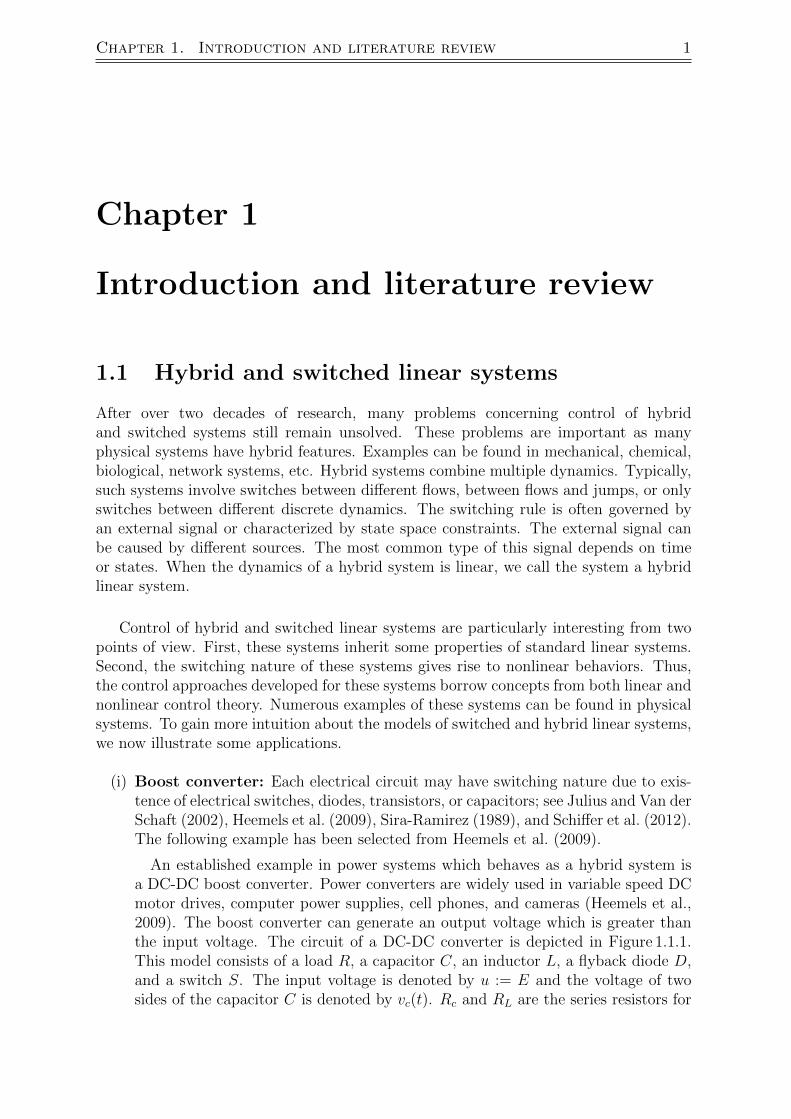
(i) Boost converter: Each electrical circuit may have switching nature due to exis-tence of electrical switches, diodes, transistors, or capacitors; see Julius and Van derSchaft (2002), Heemels et al. (2009), Sira-Ramirez (1989), and Schiffer et al. (2012).The following example has been selected from Heemels et al. (2009).
An established example in power systems which behaves as a hybrid system isa DC-DC boost converter. Power converters are widely used in variable speed DCmotor drives, computer power supplies, cell phones, and cameras (Heemels et al.,2009). The boost converter can generate an output voltage which is greater thanthe input voltage. The circuit of a DC-DC converter is depicted in Figure 1.1.1.This model consists of a load R, a capacitor C, an inductor L, a flyback diode D,and a switch S. The input voltage is denoted by u := E and the voltage of twosides of the capacitor C is denoted by vc(t). Rc and RL are the series resistors for

2 1.1. Hybrid and switched linear systems
the capacitor and the inductor, respectively. The switching period Ts for the switchS is given. The duty cycle α(t) ∈ [0, 1], that is, the ratio of the activation durationof on mode for switch S to the period Ts, is considered as the external input. Whenthe switch S is open, depending on the voltage of two sides of the flyback diode D,this diode may function in on or off modes. Now, assuming x(t) = [iL(t) vc(t)]
> asthe state variables of the boost converter, depending on the status of the diode Dand the switch S, three operation modes for this system can be investigated. Thismodel can be written in the form of
x(t) = Aσ(t,x)x(t) +Bσ(t,x)u σ(t, x) ∈ L := 1, 2, 3, (1.1)
where Ai and Bi for i ∈ L are specified as follows:
1) In the first mode the switch S is closed and the entire current iL passes throughthe switch S, thus iL > 0 or [1 0] x > 0. In this case, the matrix A1 and thevector B1 are given by
A1 =
−RLL 0
0 −1(R+Rc)C
, B1 =
1L
0
. (1.2)
The system works in this mode until time reaches to t = (n− 1 +α)Ts, wheren ∈ N. Then the system switches to mode 2).
2) In this mode the switch S is open and the flyback diode is on. Then, iL > 0or [1 0]x > 0, and the data are computed to be
A2 =
−1L
(RL + RcR
R+Rc
)−1L
RR+Rc
RC(R+Rc)
−1C(R+Rc)
, B2 =
1L
0
. (1.3)
The system can have two transitions from this mode. If iL = 0 or [1 0]x = 0holds, then the system switches to mode 3). Otherwise, after spending timeup to t = nTs the system switches to mode 1).
3) In this mode the switch S is open and the flyback diode is off. It implies thatiL = 0 or [1 0]x = 0, and
A3 =
0 0
0 −1(R+Rc)C
, B3 =
0
0
. (1.4)
The system stays in this mode until the time instance t = nTs. Afterwards,the system switches to mode 1).
As will be explained in Section 1.2, the model of the boost converter (1.1) is in theform of a controlled switched linear system. The switching rules depend on boththe states and time.

Chapter 1. Introduction and literature review 3
L
E
D
vc(t)C
α(t) → S
RL
Rc
iL(t)
R
Figure 1.1.1: A DC-DC boost converter (Heemels et al., 2009).
(ii) Mobile multi-agent systems with switching topology: This example hasbeen selected from Olfati-Saber and Murray (2004). In multi-agent systems, eachagent exchanges information with some other agents called its “neighbors”. Thiscommunication defines a network topology. The network topology is often repre-sented by a directed graph G = (V,E,A), where V = v1, . . . , vn denotes the setof nodes associated to the n agents, E ⊆ V × V is the set of edges which cor-responds to the communication between agents, and A = [aij] with non-negativeentries is the n×n adjacency matrix (Ren and Beard, 2007). The network may havea switching topology perhaps due to the agents’ changing positions or existenceof obstacles between the agents. In this case, one can associate a directed graphGk ⊆ Γ corresponding to each new topology, where Γ is a set of finite collectionsof digraphs with n nodes and k belongs to an index set L := 1, . . . , ⊂ N with := |Γ|. Then, the states of the network evolve with different dynamics, whichcan be expressed by a switched linear system in the form of
x = −Lσ(t,x)x, (1.5)
where σ : R × Rn → L is a switching signal which specifies the active network
topology. The matrix Lk = [lk,ij]n×n with k ∈ L is called the Laplacian of thegraph Gk, which is defined by
lk,ij =
⎧⎪⎪⎨⎪⎪⎩
n∑p=1, p =i
ak,ip j = i,
−ak,ij, j = i.
Note that for two different agents i, j ∈ 1, . . . , n which are not neighbors in Gk,we have ak,ij = 0 for each k ∈ L. The aim of the consensus algorithm consists incharacterizing a communication routine such that all states exponentially convergeto the same variable, namely
x1(∞) = x2(∞) = · · · = xn(∞) =1
n
n∑i=1
xi(0). (1.6)

4 1.1. Hybrid and switched linear systems
v1 v2
d1d2 d∗00
Figure 1.1.2: Schematic of the moving objects before, during, and after collision (Goebelet al., 2009).
Now, note that (1.5) defines a switched linear system, where switching signal de-pends on time and state variables.
(iii) Collisions: The system dynamics of two moving particles may change instantlywhen a collision between them occurs. More precisely, the collision may lead tosudden changes on the velocities of the mobile objects. Examples of such collisionsare billiard balls and bouncing balls (Goebel et al. (2009), Lygeros (2004) andBrogliato (1999)). We now illustrate the following example taken from Goebelet al. (2009).
Consider two particles which are moving towards each other with constant speedsv1 and v2; see Figure 1.1.2. For simplicity, let’s assume that the diameters of bothparticles are zero. The states of this system can be considered as x = [d v],where d = [d1 d2]
and v = [v1 v2] represent the positions and the velocity of the
two particles, respectively. The system dynamics are specified by Newton’s secondlaw as
x =
⎡⎢⎢⎢⎢⎢⎣d1
d2
v1
v2
⎤⎥⎥⎥⎥⎥⎦ =
⎡⎢⎢⎢⎢⎣
0 0 1 0
0 0 0 1
0 0 0 0
0 0 0 0
⎤⎥⎥⎥⎥⎦
⎡⎢⎢⎢⎢⎣d1
d2
v1
v2
⎤⎥⎥⎥⎥⎦ := Ax. (1.7)
Note that the system dynamics evolves in accordance with (1.7) whenever x ∈C := x : d1 ≤ d2. A collision occurs when the positions of the particles are thesame and v1 ≥ v2. In a collision time instance, positions of the particles remainthe same, that is, d+ = d, while the velocities can be derived by the momentumequation
m1v+1 +m2v
+2 = m1v1 +m2v2, (1.8)
and the energy dissipation equation
v+1 − v+2 = −ρ(v1 − v2), (1.9)
where m1 and m2 are the masses of the particles and the constant 0 < ρ < 1is called restitution coefficient. Thus, the model of this system for the points

Chapter 1. Introduction and literature review 5
V1:on/off
V2:on/off
T1
T2
w downstream processingv2
v1v1,max
v1,min
v2,max
v2,min
Figure 1.1.3: Schematic of the chemical process plant (Simeonova et al., 2006).
belonging to the collision set specified by D = x : d1 = d2, v1 ≥ v2 reads
⎡⎢⎢⎢⎢⎢⎣
d+1
d+2
v+1
v+2
⎤⎥⎥⎥⎥⎥⎦ =
⎡⎢⎢⎢⎢⎢⎢⎣
1 0 0 0
0 1 0 0
m1−m2ρm1+m2
m2(1+ρ)m1+m2
0 0
m1(1+ρ)m1+m2
m2−m1ρm1+m2
0 0
⎤⎥⎥⎥⎥⎥⎥⎦
⎡⎢⎢⎢⎢⎢⎣
d1
d2
v1
v2
⎤⎥⎥⎥⎥⎥⎦ := Gx. (1.10)
Consequently, we observe that the model of this system can be represented in theform of
H :
x = A x x ∈ C,
x+ = G x x ∈ D.(1.11)
We talk extensively about stability and optimal control of hybrid systems of thisform in Chapter 6.
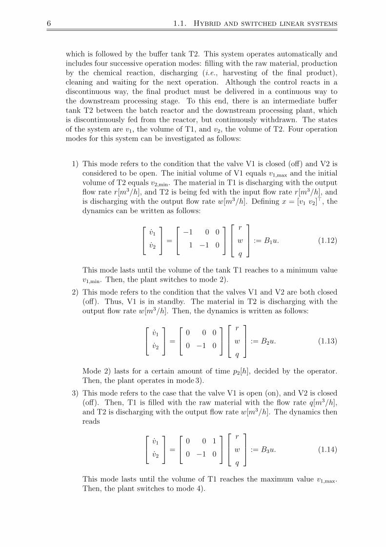
(iv) Chemical process systems: Many chemical process plants can include hybridor switching effects. For example, opening and closing of valves in a plant maysuddenly change inputs, outputs, or states of the system. Different scenarios ofinterconnection of tank systems are introduced in the literature; see Raisch et al.(1999) or Simeonova et al. (2006). The following example has been selected fromSimeonova et al. (2006).
The chemical plant depicted in Figure 1.1.3 is a simplified version of the bench-mark chemical plant (Simeonova, 2008). The tank T1 is a batch chemical reactor
6 1.1. Hybrid and switched linear systems
which is followed by the buffer tank T2. This system operates automatically andincludes four successive operation modes: filling with the raw material, productionby the chemical reaction, discharging (i.e., harvesting of the final product),cleaning and waiting for the next operation. Although the control reacts in adiscontinuous way, the final product must be delivered in a continuous way tothe downstream processing stage. To this end, there is an intermediate buffertank T2 between the batch reactor and the downstream processing plant, whichis discontinuously fed from the reactor, but continuously withdrawn. The statesof the system are v1, the volume of T1, and v2, the volume of T2. Four operationmodes for this system can be investigated as follows:
1) This mode refers to the condition that the valve V1 is closed (off) and V2 isconsidered to be open. The initial volume of V1 equals v1,max and the initialvolume of T2 equals v2,min. The material in T1 is discharging with the outputflow rate r[m3/h], and T2 is being fed with the input flow rate r[m3/h], andis discharging with the output flow rate w[m3/h]. Defining x = [v1 v2]>, thedynamics can be written as follows: v1
v2
=
−1 0 0
1 −1 0
r
w
q
:= B1u. (1.12)
This mode lasts until the volume of the tank T1 reaches to a minimum valuev1,min. Then, the plant switches to mode 2).
2) This mode refers to the condition that the valves V1 and V2 are both closed(off). Thus, V1 is in standby. The material in T2 is discharging with theoutput flow rate w[m3/h]. Then, the dynamics is written as follows: v1
v2
=
0 0 0
0 −1 0
r
w
q
:= B2u. (1.13)
Mode 2) lasts for a certain amount of time p2[h], decided by the operator.Then, the plant operates in mode 3).
3) This mode refers to the case that the valve V1 is open (on), and V2 is closed(off). Then, T1 is filled with the raw material with the flow rate q[m3/h],and T2 is discharging with the output flow rate w[m3/h]. The dynamics thenreads v1
v2
=
0 0 1
0 −1 0
r
w
q
:= B3u. (1.14)
This mode lasts until the volume of T1 reaches the maximum value v1,max.Then, the plant switches to mode 4).

Chapter 1. Introduction and literature review 7
4) This mode refers to the case that both V1 and V2 are closed (off). Only T2is discharging with the output flow rate w[m3/h]. Then, the system dynamicscan be written as follows: v1
v2
=
0 0 0
0 −1 0
r
w
q
:= B4u. (1.15)
Mode 4) lasts for certain amount of time p4[h]. Then, the plant goes againto mode 1), and the cycle continues.
Now, consider that the dynamics of the overall system can be represented as aswitched linear system of the form
x = Bσ(t,x)u σ(t, x) ∈ L := 1, 2, 3, 4, (1.16)
where σ(t, x) : R×R2 → L represents the switching signal which depends on timeand the states of the system.
1.2 Model of hybrid and switched linear systems
As the previous physical applications suggest, a hybrid linear system can be representedby the following general model:
H :
x = Aσ(t,x) x+Bσ(t,x) u x ∈ C,x+ = Gσ(t,x) x+Hσ(t,x) v x ∈ D,
(1.17)
where
σ(t, x) ∈ L := 1, . . . , `, (1.18)
indicates the switching signal between different dynamics (Ai, Bi, Gi, Hi) for i ∈ L. Inthis model, C ⊆ Rn and D ⊆ Rn denote the flow and jump sets, respectively. Notethat from the model (1.17), different models of switched linear systems can be derivedby restricting the parameters, as will be stated in the following.
(i) If D = ∅ and C = Rn, then (1.17) is converted to a continuous switched linearsystem. If σ(t, x) = σ(t), that is, the switching signal is only a function of time,then a switched linear system with arbitrary time-dependent switching signalresults. If σ(t, x) = σ(x), that is, the switching signal is only a function of thestates, then a switched linear system with state dependent switching results. Ifthe control input is not identically equal to zero, that is, Bi 6= 0 for some i ∈ L,then we refer to the system as a controlled switched linear system. Otherwise, werefer to the system simply as a switched linear system. Note that throughout thisthesis, we do not consider the switching signal as a control input.
8 1.2. Model of hybrid and switched linear systems
(ii) If C = ∅ and D = Rn, then we will arrive at a discrete time controlled switchedlinear system. Again, if the switching signal σ is only a function of time, a discretetime controlled switched linear system with arbitrary switching signal results, andif it is only a function of the states, a discrete time controlled switched linearsystem is obtained. If the control input is identically zero for all modes, then wesimply refer to the system as a discrete switched linear system.
From the above statements, we can argue that switched linear systems form a subclassof hybrid linear systems. In this dissertation we discuss different problems associatedwith stability of continuous switched linear systems and optimal control of hybrid linearsystems. Then, depending on the class of switched and hybrid systems, we study thefollowing solutions of these systems.
a) For a (controlled) switched linear system with arbitrary switching signal, weassume a finite number of switching within a finite time interval occurs. Therefore,solutions of such systems are unique for each initial condition and are always ab-solutely continuous, implying that such solutions are continuous and differentiablealmost everywhere. Moreover, these solutions follow the direction of vector fieldalmost everywhere. Thus, for switched linear systems with arbitrary switchingsignals we consider the Caratheodory solutions. For illustration of Caratheodorysolutions, see Appendix A.6.2.1 and Cortes (2008).
b) Solutions of a (controlled) switched linear system with state dependent switchingare always absolutely continuous. However, in this case a trajectory of theswitched system can slide on switching manifolds, and thus may not follow thedirection of vector field almost everywhere. For this reason, for switched linearsystems with state space constraints, we consider the Filippov solutions. For thedefinition of the Filippov solutions, see Appendix A.6.2.2, Filippov (1988), andCortes (2008). It is worth mentioning that Filippov solutions may not be uniquefor switched linear systems with state dependent switching; see Cortes (2008).
c) Solutions of a hybrid linear system can exhibit jumps. Therefore, such solutionsare absolutely continuous within flow evolutions, while they are not necessarilycontinuous during jumps; see Goebel et al. (2012). Thus, for a hybrid linear systemdue to the discontinuity of its solutions and the different nature of flow and jumpdynamics, we investigate the notion of generalized time domain for the domain ofstate variables in the hybrid system (1.17). The generalized time domain consistsof two elements as a subset of R≥0 × N0, where N0 = N ∪ 0. The first elementin the product indicates the actual time, whereas the second ingredient in theproduct counts the jump events. For system modelling and general solutions in ageneralized time domain, see Goebel et al. (2012). Similar to item b), solutions ofa hybrid linear system may not necessarily be unique.
In this dissertation, we tackle three different problems regarding control of hybrid andswitched linear systems: stability and stabilization of switched linear systems, and opti-mal control of hybrid linear systems. We now briefly elaborate these problems and point

Chapter 1. Introduction and literature review 9
out some of the previous results related to these topics. For different stability and stabi-lization problems in the contexts of discrete time linear time varying and switched linearsystems one can refer to, for example, Lin and Antsaklis (2009); Ahmadi et al. (2014);Daafouz et al. (2002); Barabanov (2005); Wirth (2005b) and the references therein.
1.3 Stability of switched linear systems
The stability problem for switched linear systems is perhaps the most well studied topicin the context of switched linear systems. The primary motivation for studying the sta-bility problem for a switched linear system perhaps stems from the fact that Hurwitzstability of constituent matrices is not sufficient for stability of the associated switchedlinear system; see Example 3.2.1 and the references therein. On the other hand, it hasalso been found that even if all matrices of a switched linear system are unstable, onemight be able to construct a routine of switching, such that some or all trajectoriesof the switched linear system exponentially converge to zero (Wicks et al., 1998). Re-search on the stability problem has given rise to many notions such as common quadraticLyapunov function (Shorten and Narendra, 2003; Wulff, 2005), single Lyapunov func-tion (De Schutter and Heemels, 2004), multiple Lyapunov functions (Branicky, 1998),converse Lyapunov theorem (Wirth, 2005a), average dwell time (Hespanha and Morse,1999), common piecewise linear Lyapunov functions (Molchanov and Pyatnitskiy, 1989),copositive Lyapunov functions for a class of rank-1 difference positive switched systemswith arbitrary number of subsystems (Fornasini and Valcher, 2010), etc. In the follow-ing, we briefly represent those approaches which are most closely related to the resultsin this thesis.
1.3.1 Common Quadratic Lyapunov function (CQLF)
The existence of a common quadratic Lyapunov function guarantees exponential stabilityof a switched linear system both under arbitrary and state dependent switching; see,e.g., Griggs et al. (2010). Moreover, it is known that quadratic stability exhibit robustproperties in terms of perturbations of constituent matrices and discretization of switchedlinear systems; see Rossi et al. (2011) and Shorten et al. (2007). The quadratic stabilityproblem for a switched system with arbitrary switching signal can be stated as follows:
Problem 1.3.1. Consider the switched linear system
x = Aσ(t)x(t) σ(t) ∈ L := 1, . . . , `, (1.19)
where all matrices Ai for i ∈ L are Hurwitz and σ is the switching signal between theAi’s. Find conditions on the real matrices Ai ∈ A := A1, . . . , A` such that the switchedsystem (1.19) is quadratically stable, that is, there exists a common quadratic Lyapunovfunction V (x) = x>Px with P = P> > 0 such that
A>i P + PAi < 0 ∀i ∈ 1, . . . , `. (1.20)

10 1.3. Stability of switched linear systems
Note that (1.20) is a linear matrix inequality (LMI) and a common Lyapunov solutionP can be computed numerically. It is known that a set of Hurwitz matrices similar to
1) set of upper (lower) triangular matrices (Shorten and Narendra, 1998),
2) set of pairwise commuting matrices (Narendra and Balakrishnan, 1994),
3) set of matrices which belong to solvable Lie Algebraic conditions (Liberzon et al.,1999; Agrachev and Liberzon, 2001),
4) set of real diagonalizable matrices which any pair of them share at least (n − 1)right eigenvectors (Shorten and Cairbre, 2001),
are classes of matrices that a common quadratic Lyapunov function for the associatedswitched linear system exists. Now, we point out two other important results which arerelated to the stability concepts introduced in Chapters 4 and 5 of this thesis.
1) Rank-1 difference switched systems: One of the well-known results in thecontext of quadratic stability is expressed by the next theorem.
Theorem 1.3.1. (See Shorten and Narendra (2003)) Consider the switched linearsystem
x =
(A− σ(t)
bc
d
)x σ(t) ∈ 0, 1, (1.21)
where A ∈ Rn×n is Hurwitz, b ∈ Rn, c> ∈ Rn, and d > 0 is a scalar. Then, thefollowing statements are equivalent:
a) The switched system (1.21) is quadratically stable,
b) The transfer function g(s) = c(sI − A)−1b+ d is strictly positive real,
c) The matrix A(A− bc
d
)has no real negative eigenvalue.
The proof of this theorem uses the Kalman-Yakubovic-Popov lemma proposedfor strictly positive real systems to guarantee the existence of a CQLF (Shortenand Narendra, 2003). This result has been proven and extended to the class ofcomplex matrices separately by Laffey (2009) and King and Nathanson (2006).
2) Two dimensional switched systems: For a pair of two dimensional matrices,existence of a CQLF is expressed by the following result:
Theorem 1.3.2. (See Shorten and Narendra (2002)) Suppose in Problem 1.3.1 ` =2, and A1, A2 ∈ R2×2 are Hurwitz. Then the switched system (1.19) is quadraticallystable if and only if the matrices A1A2 and A1A
−12 do not have any real negative
eigenvalue.
Stability of second order switched systems including two subsystems under singularperturbations has been considered by El Hachemi et al. (2011).
Despite much effort similar results for matrices with higher dimensions have onlybeen derived recently (Kouhi et al., 2013a).

Chapter 1. Introduction and literature review 11
1.4 Stabilization of switched linear systems
The stabilization problem for switched linear systems has been studied from diversepoints of view. Some research considers stabilization of the switched system (1.19)with Hurwitz constituent matrices, by restricting the rate of the switching signal. Moreprecisely, when all matrix constituents are Hurwitz, it is shown that if the switchingevents are sufficiently far apart in time, then the switched linear system will be stable.This concept is well-known as stability with average dwell time. Finding a reasonableupper bound for the average dwell time has been investigated in Hespanha and Morse(1999), Solo (1994), Geromel and Colaneri (2006), and Chesi et al. (2012). Some otherresearch assumes that the matrices Ai for all i ∈ L in (1.19) are not necessarily stable,and they look for a switching law that makes the switched system exponentially stable(Wicks et al., 1998; Feron, 1996). In this dissertation, however, we follow a standardapproach for quadratic stabilization of a controlled switched linear system using localstate feedback for each mode, similar to Cheng (2004) and De Schutter and Heemels(2004). This problem for a controlled switched system with arbitrary switching signalcan be stated as follows:
Problem 1.4.1. Consider the controlled switched system
x = Aσ(t) x(t) +Bσ(t) u(t) σ(t) ∈ L := 1, . . . , `. (1.22)
Find a local state feedback u = Kσ(t)x such that the resulting closed loop switchedsystem
x =(Aσ(t) +Bσ(t)Kσ(t)
)x, (1.23)
is quadratically stable, that is, there exists a common quadratic Lyapunov functionV (x) = x>Px with P = P> > 0 such that
(Ai +BiKi)>P + P (Ai +BiKi) < 0 ∀i ∈ L. (1.24)
Note that (1.24) is not an LMI due to the existence of the coefficient PBiKi in theinequality, where both P and Ki are unknown parameters. Nevertheless, one can convertthis inequality to the LMI form as follows; see De Schutter and Heemels (2004). Firstby pre-multiplying by P−1 and post-multiplying by P−1, we get
(P−1A>i + P−1K>i B>i ) + (AiP
−1 +BiKiP−1) < 0 ∀i ∈ L. (1.25)
Thus with the assumptions X := P−1 and Yi := KiP−1, we can rewrite (1.25) as
XA>i + AiX + Y >i B>i +BiYi < 0 ∀i ∈ L. (1.26)
Now, it is evident that (1.26) is an LMI and can be solved numerically. However,numerical methods do not provide any insight into the feasibility of such LMI’s. Forthis reason, finding sufficient conditions on Ai and Bi for all i ∈ L under which thesolvability of these LMI’s is guaranteed, is a crucial problem. Several articles dealing
12 1.5. Optimal control of hybrid linear systems
with this problem have been published, e.g., Cheng (2004); Sun and Zheng (2001). Forexample, in Cheng (2004) a necessary and sufficient condition for stabilization of secondorder controlled switched linear systems with single input has been explored.
In this dissertation, we consider stabilization of a class of controlled switched linearsystems where all open loop matrices Ai’s, i ∈ L, share a right invariant subspacewith appropriate dimension to which a common quadratic Lyapunov function can beassociated. Satisfying some rank conditions with respect to Bi’s, for this class weshow that quadratic stabilization can be achieved if sufficient number of input channelsare available. Moreover, we demonstrate that this approach can be employed forstabilization of a class of controlled switched systems, where their open loop matriceshave invariant subspaces which have sufficiently small distances, and a certain form ofRiccati inequalities for the matrices associated with these invariant subspaces hold.
The concept of common controlled invariant subspaces has been previously consideredin the context of linear parameter varying and switched linear systems, often for stabilityof a system in a subspace of the state space or for mode decoupling; see, e.g., Balas et al.(2003), Yurtseven et al. (2010), Haimovich and Braslavsky (2010), and Blanchini (1999).Furthermore, it has also been used for determining a sequence of stabilizable controlledswitched linear systems (Sun and Zheng, 2001). For these purposes, algorithms havebeen developed to compute a largest common controlled invariant subspace of a switchedsystem for a subspace of x ∈ X ⊆ Rn and u ∈ U. The largest common invariant subspacefor such a switched linear system can be computed by an iterative algorithm using fixedpoint theory; see, e.g., Tsatsomeros (2001) and Julius and Van der Schaft (2002).
1.5 Optimal control of hybrid linear systems
Optimal control problems for hybrid systems are recognized as challenging mathematicalproblems. In such problems, one often associates several cost values each of whichcorresponds to a part of a trajectory evolving with a given dynamics. Then, the objectiveis to minimize the sum of these costs over a fixed or free time interval, and fixed or freeswitching time instances. For such optimal control problems, the maximum principlefor hybrid systems holds; see Sussmann (1999); Caines et al. (2006); Azhmyakov et al.(2007); Liberzon (2011); Passenberg et al. (2011). In one of the early works by Sussmann(1999), a general condition for the maximum principle for hybrid systems including fixedswitching sequences and free switching time instances has been proposed. In Caineset al. (2006) the concept is generalized to a setting with guard conditions. Typically,such algorithms extend the classical maximum principle by additional requirements onthe switching manifolds known as transversality conditions. Despite the sound theory,computational difficulties arise even in a setting with quadratic costs for hybrid linearsystems (Riedinger et al., 1999; Azhmyakov et al., 2009; Xu and Antsaklis, 2004).
Linear quadratic regulator (LQR) problems for hybrid and switched linear systems,similar to optimal control problems for the general form of hybrid systems, may havefixed or free switching times, and fixed or free switching sequences; see, for instance,Problem 6.5.1 as a possible scenario. Several results dealing with these problems exist

Chapter 1. Introduction and literature review 13
in the literature (Xu and Antsaklis, 2004; Azhmyakov et al., 2009). For instance, in Xuand Antsaklis (2004), an efficient numerical algorithm for the LQR problem with freeswitching times is obtained by introducing a parameterization in terms of switchingtimes.
Some other research provides numerical solutions for optimal control of systemswhich are closely related to hybrid linear systems. For example, in the context ofpiecewise linear systems, Rantzer and Johansson (2000) suggests lower and upperbounds to the optimal cost by formulating a semi-definite and a convex programmingproblem. Analytic expressions for sub-optimal solutions to an LQR problem for LTI sys-tems with state space and input constraints have been reported in Johansen et al. (2002).
1.6 Organization of the thesis
In Chapter 2, we study different approaches concerning left eigenstructure assignmentfor multi-input systems, pole placement for single input systems, and partial poleplacement for single- and multi-input systems. This chapter can be viewed as the basisfor the upcoming results on the stability and stabilization of switched linear systemsin Chapter 3 and Chapter 4. Moreover, this chapter extends the result by Kouhi andBajcinca (2011a) on left eigenstructure assignment.
In Chapter 3, we study exponential stability and stabilization of switched linearsystems with state dependent switching signals. In these problem settings, we assumecertain restrictions on the geometry of switching manifolds. This chapter extends partsof the results by Kouhi and Bajcinca (2011b) on exponential stability and stabilizationof switched linear systems. Our techniques use the concept of common left eigenvectorsand left eigenstructure assignment introduced in Chapter 2.
In Chapter 4, we apply the concept of common eigenvectors and left eigenstructureassignment for stability and stabilization of switched linear systems under arbitraryswitching. Our approach for stabilization investigates a local state feedback designfor each subsystem of a controlled switched system. The main result in this chapterdiscusses stabilization of a controlled switched system whose open loop constituentmatrices share an invariant subspace to which a common quadratic Lyapunov functioncan be associated. We then use the left eigenstructure assignment technique forimposing a number of desired left eigenvectors that are perpendicular to the commoninvariant subspace, thereby guaranteeing quadratic stability of the closed loop matricesof subsystems. Moreover, we discuss robust stability of a switched linear system whenits Hurwitz matrices share (n− 1) real left eigenvectors. This chapter extends the resultby Kouhi and Bajcinca (2011c) on quadratic stability and stabilization of switchedlinear systems.
In Chapter 5, we extend the results by Shorten and Narendra (2003) on quadraticstability, and Shorten et al. (2009) concerning weak quadratic stability of switching

14 1.6. Organization of the thesis
systems with two modes and rank-1 difference matrices. We show that their resultscan be extended to switched systems with rank m ≥ 1 difference matrices, providedthat a symmetric transfer function matrix can be associated with the pair of matrices.Moreover, we use this approach for computing a set of control inputs which stabilize aclass of controlled switched linear systems. Parts of these results have been publishedin Kouhi et al. (2013a) and Kouhi et al. (2014).
In Chapter 6, we briefly study the stability problem for hybrid linear systems. Weshow that their stability is equivalent to stability of switched linear systems, if bilineartransformations for converting discrete evolutions to continuous dynamics are used.The main results of this chapter, however, are related to the optimal control of hybridlinear systems. We investigate two problem configurations. In the first scenario, theclass of hybrid linear systems is specified by a single flow and a single jump dynamics,and state space constraints are represented by polyhedral sets. For this system, weconsider an optimal control problem with a fixed sequence of switching occurringat fixed time instances. Our solution algorithm determines upper and lower boundsfor the overall cost function of this problem. In the next scenario, we consider anoptimal control problem for hybrid linear systems including multiple flow dynamicswith fixed sequence of switching, such that switches can take place at free timeinstances. This result solves a problem related to maximum principle for hybrid linearsystems. Parts of the results in this chapter have been published by Kouhi et al. (2013b).
In Chapter 7, we provide the conclusions.
In Appendix A, some necessary definitions and existing concepts are given to makethis dissertation necessarily self-contained.

Chapter 2. Left eigenstructure assignment 15
Chapter 2
Left eigenstructure assignment
2.1 Introduction
Eigenstructure assignment for multi-input systems and pole placement for single-inputsystems using static state feedback are old topics in the control systems theory. From aclassical point of view, pole placement for a single input system is often used to assignsome or all eigenvalues of a linear system to stabilize the closed loop system, and/or toimprove the rate of convergence of system solutions (Kailath, 1980; Saad, 1986). Formulti-input systems, due to more freedom on control inputs, eigenstructure assignmenthas given rise to different problem formulations. For example, right eigenstructureassignment is used to shape the solutions of a linear system (Wonham, 1967; Liuand Patton, 1998), and left eigenstructure is used for disturbance attenuation (Choi,1998a,b). In this chapter, however, our motivation is not to provide new results in thissense, nor to be involved fundamentally in different eigenstructure assignment methodsfor LTI systems. Although some of the techniques introduced in this chapter can beused for control of a linear system, some others essentially may not make sense for thispurpose. In fact, the current chapter should be viewed as an introduction for the resultsof the upcoming chapters on stabilization of controlled switched linear systems.
Our main interest in this chapter is how to exploit the potential of control inputs forassigning as many desired left eigenvectors as possible using state feedback, such thatthe closed loop system is stable. It should be mentioned that this aim is different fromconventional left eigenstructure assignment proposed in the literature, including Choi(1998a,b) and the references therein.
2.2 Left eigenvector assignment
First, we present left eigenstructure assignment for single input systems. Then, in thenext part we extend this to multi-input systems.
16 2.2. Left eigenvector assignment
2.2.1 Single-input systems
Consider a single input controllable LTI system given by the state space representation
x = Ax+ bu, (2.1)
where x ∈ Rn and u ∈ R are the state vector and the control input, respectively. Supposewe aim at designing a state feedback u = kx, where k is a row vector, for assigning adesired left eigenvector w ∈ Cn and its corresponding eigenvalue λ1 ∈ C<0 to the closedloop system, where C<0 denotes the open left half plane. Then, by a simple computationwe have
w∗(A+ bk) = λ1w∗ =⇒ k = −w
∗(A− λ1I)
w∗bfor w∗b 6= 0. (2.2)
The left eigenvector w appears nonlinearly in the closed loop system matrix Acl = A+bkas
Acl =
(I − bw∗
w∗b
)A+ λ1
bw∗
w∗b. (2.3)
Note that the matrix I−bw∗/w∗b in (2.3) has one eigenvalue equal to 0 with correspond-ing left eigenvector c1 := w, and n − 1 eigenvalues equal to 1 with corresponding lefteigenvectors ci such that c>i b = 0 for i ∈ 2, . . . , n. Now, a natural problem arising fromthe gain (2.2) and the closed loop description (2.3) is to explore the proper selection ofw and λ1 such that k> ∈ Rn and Acl is a Hurwitz matrix (Kouhi and Bajcinca, 2011a).
Lemma 2.2.1. (Simon and Mitter, 1968) The characteristic polynomial of the closedloop system (2.3) is given by
det (λI − Acl) = (λ− λ1)w∗adj(λI − A)b
w∗b= (λ− λ1)(λn−1 + β1λ
n−2 + · · ·+ βn−1), (2.4)
where the coefficients βi for i ∈ 1, . . . , n− 1 are in the form of
βi =w∗(aiI + ai−1A+ ai−2A
2 + · · ·+ Ai)b
w∗b, (2.5)
and ai for i ∈ 1, 2, . . . , n are the coefficients of the characteristic polynomial of A,i.e., p(λ) = det(λI − A) = λn + a1λ
n−1 + · · ·+ an−1λ+ an.
Proof: The characteristic polynomial of the closed loop system matrix Acl is computedas follows:
det(λI − A− bk) = det(λI − A)det[I − (λI − A)−1bk]
= p(λ) det[I − (λI − A)−1bk
]= p(λ)
[1− k(λI − A)−1b
]= p(λ)
[1 +
w∗(A− λ1I)(λI − A)−1b
w∗b
]= p(λ)
[w∗(λI − A− λ1I + A)(λI − A)−1b
w∗b
]= (λ− λ1)
w∗adj(λI − A)b
w∗b.

Chapter 2. Left eigenstructure assignment 17
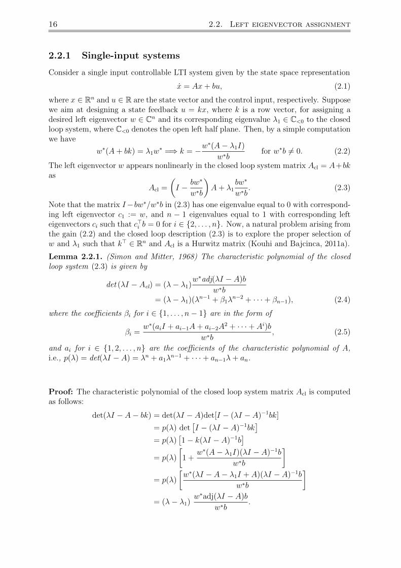
b
(a1 I + A)bΩ
Figure 2.2.1: The interior of the colored region, denoted by Ω, is the proper region forselection of a desired left eigenvector w, when n = 2.
Note that in deriving the last line we used the fact
p(λ)(λI − A)−1 = det(λI − A).(λI − A)−1 = adj(λI − A);
see also AppendixA.2 and Kailath (1980). On the other hand, the Resolvent formula(Kailath, 1980) for the adjoint matrix is given by
adj(λI − A) = An−1 + (λ+ a1)An−2 + · · ·+
(λn−1 + a1λn−2 + · · ·+ an−1)I
= λn−1I + λn−2(a1I + A) + · · ·+ (an−1I + · · ·+ a1An−2 + An−1). (2.6)
Pre-multiplying equation (2.6) by w∗ and post-multiplying by b, and dividing it by w∗bleads to the formulation (2.5).
Now, consider that deriving a simple statement for stability of Acl from the polyno-mial (2.4) based on the Routh-Hurwitz stability criteria is not straightforward. There-fore, we will study this problem in more detail in the sequel. However, in the cases whenn = 2 or n = 3, and λ1 and consequently w are real, we can get particularly simpleillustrative results. For instance, with n = 2, λ1 ∈ R<0, and w ∈ R
2, stability of Acl isequivalent to have
β1 =w(a1I + A)b
wb> 0. (2.7)
This inequality holds if the inner-products of w with b, and w with (a1I +A)b share thesame sign. Hence, the set of all desired left eigenvectors w that makes β1 > 0 can bespecified geometrically, as illustrated by the shaded area Ω in Figure 2.2.1. If n = 3,λ1 ∈ R<0, and w ∈ R
3, then in addition to (2.7), we require
β2 =w(a2I + a1A+ A2)b
wb> 0. (2.8)
Again, the two expressions β1 > 0 and β2 > 0 with respect to the parameter wcharacterize a region in the three dimensional state space. This region can be computedgeometrically (Kouhi and Bajcinca, 2011b).

18 2.2. Left eigenvector assignment
2.2.1.1 Closed loop stability
To solve the problem of selecting a suitable w which stabilizes the closed loop matrixAcl for the general case, we use the linear transformation z = Tx. Then, the closed loopsystem x = (A+ bk)x is converted to the form
z = (Ac + bckc)z, Ac = T−1AT, bc = T−1b, and kc = kT. (2.9)
Consider now the particular case where Ac and bc are in controllable canonical form
Ac =
0 1 0 . . . 00 0 1 . . . 0. . . . .. . . . .. . . . .0 0 0 . . . 1−an −an−1 −an−2 . . . −a1
, bc =
00...01
. (2.10)
Note that for any controllable pair (A, b) this transformation matrix T exists, and isgiven by
T = Φc(A, b)Φ−1c (Ac, bc), (2.11)
where Φc(A, b) and Φc(Ac, bc) are the controllability matrices of the original and of thetransformed systems, respectively. Now, referring to (2.4), the closed loop characteristicpolynomial for the closed loop matrix Ac,cl = Ac + bckc reads
det(λI − Ac,cl) = (λ− λ1)w∗cadj(λI − Ac)bc
w∗cbc,
where wc = [wc,1 . . . wc,n]> is the left eigenvector for the matrix Ac,cl corresponding tothe eigenvalue λ1. On the other hand, one can observe that the closed loop matrix Ac,cl
is also in canonical form
Ac,cl =
0 1 · · · 0
0 0 · · · 0
......
......
0 0 · · · 1
λ1w∗c,1w∗c,n
−w∗c,1+λ1w∗c,2w∗c,n
· · · −w∗c,(n−1)
+λ1w∗c,n
w∗c,n
.
As bc in (2.10) has only one non-zero element, for computing w∗cadj(λI − Ac)bc we onlyrequire to compute the n’th column of adj(λI−Ac). Note that w∗cbc = w∗c,n 6= 0 indicatesthat w∗c,n 6= 0. Thus, the characteristic polynomial of Ac,cl equals
det(λI − Ac,cl) =
= λn +1
w∗c,n
(w∗c,(n−1) − λ1w
∗c,n
)λn−1 + · · · − 1
w∗c,nλ1w
∗c,1
=1
w∗c,n(λ− λ1)
(w∗c,nλ
n−1 + w∗c,(n−1)λn−2 + · · ·+ w∗c,2λ+ w∗c,1
). (2.12)
Chapter 2. Left eigenstructure assignment 19
The last equation reveals the fact that the characteristic polynomial of Ac,cl does not de-pend on the variables a1, a2, . . . , an, but it is determined by the parameters wc,1, . . . , wc,n,and λ1. Therefore, a left eigenvector wc which stabilizes Ac,cl can be characterized bythe coefficients of the following stable polynomial
hc(λ) = w∗c,nλn−1 + w∗c,(n−1)λ
n−1 + · · ·+ w∗c,2λ+ w∗c,1. (2.13)
On the other hand, from the transformation Ac,cl = T−1AclT , it is simple to show thatw = (T ∗)−1 wc. Thus, after finding an appropriate wc from (2.13), we can compute avector w which stabilizes Acl = A+ bk (Kouhi and Bajcinca, 2011a). In the case, whenλ1 is not real, for having a real feedback gain k the eigenvalues of the closed loop matrixAcl must come in complex conjugate pairs. This implies that hc(λ) must have the formof hc(λ) = w∗c,n(λ− λ∗1)hc,1(λ), where hc,1(λ) is a polynomial with real coefficients.
When λ1 and wc are restricted to be real, several contributions in the literatureare available that specify simple sufficient conditions for stability of polynomials in theform of (2.13); for example, the results by Craven and Csordas (1998) and Dimitrovand Pena (2005). Now, we stress one of these results in the next lemma.
Lemma 2.2.2. (See Dimitrov and Pena (2005)). Let γ be the unique real root of thepolynomial γ3−5γ2 +4γ−1 = 0, namely γ = 4.0796. If the coefficients of the polynomialhc(λ) defined by (2.13) are all positive real and the following conditions hold
wc,iwc,i+1 ≥ γwc,i−1wc,i+2 ∀i ∈ 2, . . . , n− 2, (2.14)
then hc(λ) is Hurwitz.
For other results on stability of polynomials, see Katkova and Vishnyakova (2008)and the references therein.
2.2.1.2 Pole placement
In this section, we show that (2.11) and (2.12) can be additionally used for pole place-ment; see Kouhi and Bajcinca (2011a). To this end, consider a controllable linear system(2.1), and let λ1, . . . , λn be a set of numbers including complex conjugate pairs. Wewish to design a state feedback law u = kx, with k> ∈ Rn, which assigns the desiredeigenvalues λi for all i ∈ 1, . . . , n to the closed loop matrix Acl = A+ bk. We performthe following algorithm for achieving this goal.
a) Obtain an appropriate canonical left eigenvector wc corresponding to λ1 from thefollowing relationship
1
w∗c,n
(w∗c,nλ
n−1 + w∗c,(n−2)λn−1 + · · ·+ w∗c,2λ+ w∗c,1
)= (λ− λ2) . . . (λ− λn). (2.15)
b) Obtain the transformation matrix T defined in accordance with (2.11).

20 2.2. Left eigenvector assignment
c) Obtain the desired feedback gain from
k = −w∗cT−1(A− λ1I)
w∗cbc. (2.16)
Note that (2.16) results by inserting the equation w = (T ∗)−1 wc into (2.2).
2.2.1.3 Single shift eigenvalue
Consider again the (not necessarily controllable) linear system (2.1). Suppose the aim isto design a state feedback u = kx that only shifts the real eigenvalue µ1 of the open loopmatrix A and replaces it by a real desired number λ1, while the other eigenvalues of Aremain unchanged. To this end, we choose the open loop left eigenvector w correspondingto the eigenvalue µ1, that is, w>A = µ1w
>, to be the desired left eigenvector for Acl
corresponding to the desired eigenvalue λ1. Then, referring to the computation (2.2),the formula for the appropriate feedback gain reads
k = −w>(A− λ1I)
w>b= −(µ1 − λ1)w>
w>bfor w>b 6= 0. (2.17)
The closed loop characteristic polynomial then will be computed by (2.4). On the otherhand, by following the same procedure on derivation of (2.4), one can argue that theopen loop characteristic polynomial p(λ) equals
p(λ) = (λ− µ1)w>adj(λI − A)b
w>b. (2.18)
Comparing (2.4) and (2.18), we conclude that except one eigenvalue, all other eigenval-ues of the closed loop and open loop matrices are the same.
The single shift eigenvalue technique has been introduced by Simon and Mitter(1968).
2.2.1.4 Partial pole placement
Consider now the linear system (2.1), with controllability of the system to be discussedin the sequel. We want to study the problem of designing a state feedback u = kx thatonly shifts the eigenvalues µ1, . . . , µm of the open loop matrix A, and replaces them bythe desired numbers λ1, . . . , λm for some 1 < m ≤ n, while keeping the other eigenvaluesof A, namely µm+1, . . . , µn, unchanged. To this end, we follow an algorithm introducedby Saad (1986). Let us denote the real Schur decomposition of A> as
A> =[Q1 Q2
] [ L>1 ?
0 L>2
][Q>1
Q>2
], (2.19)
where columns of T = [Q1 Q2] ∈ Rn×n consist of orthonormal vectors, L1 ∈ Rm×m, andL2 ∈ R(n−m)×(n−m); see (Stewart, 2001) and Appendix A.2.9. As T is orthonormal, thatis, T−1 = T>, (2.19) reveals that eigenvalues of L1 are equal to m eigenvalues of A, and

Chapter 2. Left eigenstructure assignment 21
eigenvalues of L2 are the same as other n−m eigenvalues of A. Without loss of generality,let us assume that the set of eigenvalues of L1 and L2 are given by µ1, . . . , µm andµm+1, . . . , µn, respectively. Note that (2.19) implies the following relationships hold:
Q>1 A = L1Q>1 and Q>2 AQ2 = L2. (2.20)
Further, introducing the parametrization k = ηQ>1 , where η> ∈ Rm, we use the trans-formation x = Tz and (2.20) to get the similarity condition
Acl := A+ bk ∼ T>AclT =
[L1 +Q>1 bη 0
? L2
]. (2.21)
This is an indication that the set of eigenvalues µm+1, . . . , µn in Acl remain unchanged,as the eigenvalues of L2 are µm+1, . . . , µn. However, the eigenvalues µ1, . . . , µm can bechanged by means of the parameter η in the term L1 + Q>1 bη. Now, we can employour pole placement technique elaborated in Section 2.2.1.2 in the upper left block forassigning the desired eigenvalues λ1, . . . , λm. To this end, define Lc,1 and bc,L1 to be thecanonical controllable form of L1 and Q>1 b, respectively. Then, we adopt the formula(2.16) for computing η as
η = −w∗c,L1
T−1L1
(L1 − λ1I)
w∗c,L1bc,L1
, (2.22)
where TL1 = Φc(L1, Q>1 b)Φ
−1c (Lc,1, bc,L1), and wc,L1 is the left eigenvector of the matrix
Lc,1 corresponding to the eigenvalue λ1. Note that η in (2.22) exists if the pair (L1, Q>1 b)
is controllable, or the controllability matrix Φc(L1, Q>1 b) has full rank. In fact, by the
definition of the controllability matrix, we have
Φc(L1, Q>1 b) = [Q>1 b L1Q
>1 b . . . (L1)m−1Q>1 b]
= Q>1 [b Ab . . . Am−1b]. (2.23)
Therefore, if
rank(Q>1 [b Ab . . . Am−1b]
)= m,
then partial pole placement is possible.
2.2.2 Multi-input systems
In this section, we generalize the results of single input systems to multi-input systemsin the form of
x = Ax+Bu, (2.24)
where x ∈ Rn and u ∈ Rm are again the state and the control input vectors, respectively.Let wi ∈ Cn for i ∈ 1, . . . ,m be m linearly independent vectors including complexconjugate pairs, and let λi ∈ C<0 for i ∈ 1, . . . ,m be numbers coming in complexconjugate pairs. Define W = [w1 . . . wm] and Λ = diag([λ1, . . . , λm]). Suppose we aim atcomputing a state feedback u = Kx with K ∈ Rm×n, such that the closed loop matrixAcl = A+BK has m assigned left eigenvectors given by the columns of W corresponding
22 2.2. Left eigenvector assignment
to m desired eigenvalues given by the diagonal entries of Λ. It is simple to show thatsuch feedback gain has the form
K = −(W ∗B)−1(W ∗A− ΛW ∗) for det(W ∗B) 6= 0. (2.25)
This design leads to the closed loop system matrix
Acl =(I −B(W ∗B)−1W ∗)A+B(W ∗B)−1ΛW ∗. (2.26)
Note that the columns of −(W ∗B)−1 and the rows of W ∗A− ΛW ∗ consist of conjugatepairs of complex vectors and thus their multiplication, K defined by (2.25), is a realmatrix. The matrix I − B(W ∗B)−1W ∗ in (2.26) has m eigenvalues equal to 0 withcorresponding left eigenvectors ci := wi for i ∈ 1, . . . ,m, and (n−m) eigenvalues equalto 1 with corresponding left eigenvectors ci such that c>i B = 0 for i ∈ m + 1, . . . , n(Kouhi and Bajcinca, 2011a). Now, we explore under which conditions the closed loopdescription Acl given by (2.26) is Hurwitz.
Lemma 2.2.3. (See Kouhi and Bajcinca (2011a)). The characteristic polynomial of theclosed loop system matrix (2.26) is given by
det (λI − Acl) = det(λI − A)1−m det(λI − Λ)W ∗adj(λI − A)B
det(W ∗B). (2.27)
Proof: Defining p(λ) = det(λI − A), the characteristic polynomial of the closed loopsystem is computed as follows:
det(λI −A−BK) = det(λI − A)det[I − (λI − A)−1BK]
= p(λ) det[I − (λI − A)−1BK
]= p(λ) det
[I −K(λI − A)−1B
]= p(λ) det
[I + (W ∗B)−1(W ∗A− ΛW ∗)(λI − A)−1B
]= p(λ) det
((W ∗B)−1
[W ∗B + (W ∗A− ΛW ∗)(λI − A)−1B
])= p(λ) det
((W ∗B)−1
)det([W ∗(λI − A) +W ∗A− ΛW ∗](λI − A)−1B
)= p(λ)
det(λI − Λ).det (W ∗(λI − A)−1B)
det(W ∗B)
= p(λ)1−m det(λI − Λ)det (W ∗adj(λI − A)B)
det(W ∗B),
where in deriving the third line of the proof, we used the general identity
det(In −XY ) = det (Im − Y X),
for any two matrices X ∈ Cn×m and Y ∈ Cm×n; see Appendix A.2.3.
Therefore, for closed loop stability, we propose the following corollary.
Corollary 2.2.1. Assume λi ∈ C<0 for all i ∈ 1, . . . ,m, det(W ∗B) 6= 0, and(A,B) is controllable. The closed loop matrix (2.26) is Hurwitz if and only ifdet (W ∗adj(λI − A)B) has no zero in the closed right half plane.

Chapter 2. Left eigenstructure assignment 23
2.2.2.1 Closed loop stability having (n− 1) inputs
Although designing a convenient W which stabilizes the closed loop system matrix (2.26)for a general m is not straightforward, we introduce a method for the case m = n − 1and W ∈ Rn×(n−1), based on the results by Kouhi and Bajcinca (2011c). Supposethe controller gain K ∈ R(n−1)×n in the form of (2.25) imposes a pre-specified set of(n − 1) linearly independent common real left eigenvectors given by the columns ofW = [w1 . . . wn−1] and the corresponding negative real eigenvalues given by the diagonalentries of Λ = diag([λ1, . . . , λn−1]) to the closed loop system matrix Acl = A + BK.For the closed loop stability, we need to ensure that the last eigenvalue λn is negativereal. Note that λn must be real because a real matrix cannot have only one complexeigenvalue with non-zero imaginary part. Now, let the characteristic polynomials of theopen and closed loop system (2.24) be denoted by p(λ) and q(λ), respectively, that is,
p(λ) = λn + a1λn−1 + · · ·+ an, (2.28)
q(λ) = λn + α1λn−1 + · · ·+ αn. (2.29)
It is a known fact that −α1 in (2.29) is equal to the sum of the closed loop eigenvalues,and simultaneously is equal to the trace of Acl, that is,
tr(Acl) =n∑i=1
λi = −α1;
see Appendix A.2.6 and Kailath (1980). Hence, λn can now be computed as
λn = −α1 −n−1∑i=1
λi = tr(Acl)− tr (Λ) . (2.30)
Further, we compute tr(Acl) from (2.26)
tr(Acl) = tr((I −B(W>B)−1W>)A+B(W>B)−1ΛW>)
= tr(A)− tr(B(W>B)−1W>A
)+ tr
(B(W>B)−1ΛW>) .
Using the identity tr(EF ) = tr(FE) for general matrices E and F , as well as the factthat tr(A) = −a1 = −tr (a1/(n− 1) In−1) = −tr
(a1/(n− 1) (W>B)−1W>B
), we have
tr(Acl) = −a1 − tr(W>AB(W>B)−1
)+ tr
(W>B(W>B)−1Λ
)= −tr
(W> (a1/(n− 1) In + A)B(W>B)−1
)+ tr(Λ).
Consequently, recalling (2.30), we can derive a simple expression for λn
λn = −tr(W>(a1/(n− 1) In + A)B(W>B)−1
). (2.31)
In the sequel we provide an algorithm for designing a matrix W which satisfies λn < 0.To this end, let θ ∈ Rn be a vector belonging to ker(B>), that is,
θ>B = 0, (2.32)
24 2.2. Left eigenvector assignment
and consider the parametrization
W> =W> + µθ>, (2.33)
where W is an arbitrary matrix in Rn×(n−1) and µ ∈ Rn−1 is an unknown vector whichmust be determined. From the definition of θ, it is obvious that
(W>B)−1 = (W>B)−1.
Defining the matrix X ∈ Rn×(n−1) and the vector Y ∈ Rn−1 as
X =(a1/(n− 1) In + A
)B(W>B)−1,
Y > = θ>(a1/(n− 1) In + A
)B(W>B)−1, (2.34)
and substituting W> from (2.33) into (2.31), we get
λn = −tr((W> + µθ>) (a1/(n− 1) In + A)B(W>B)−1
)= −tr (W>X)− tr (µY >).
As θ, µ, and Y are vectors, we can write
tr(µY >) = tr(Y >µ) = Y >µ,
which leads to
λn = −tr (W>X)− Y >µ. (2.35)
Thus, the last equation indicates that the requirement λn < 0 is equivalent to have
Y >µ > −tr (W>X). (2.36)
Note that if we fix W , then X and Y will be known variables. Then, (2.36) representsan inequality with µ as an unknown variable. This inequality indicates that theinner-product of the known vector Y and the unknown vector µ must be greaterthan the known scalar −tr (W>X). The set of vectors µ fulfilling such charac-teristics indeed identifies a geometric cone in the space Rn−1. Now, sweeping overall possibleW ∈ Rn×(n−1) would yield the region Ω ⊆ Rn×(n−1) of all desired matrices W .
In the following example, we explain how we can compute an appropriate W basedon the proposed algorithm.
Example 2.2.1. Consider the controlled linear system (2.24) with
A =
3 −3 −70 −4 01 3 −5
, B =
1 11 02 2
. (2.37)
A has eigenvalues at 2,−4,−4, and thus is not Hurwitz. Suppose we want to determinea state feedback gain K ∈ R2×3 which assigns two eigenvalues at −2,−3, and makesthe closed loop matrix Acl = A + BK Hurwitz. To this end, we assume that the left
Chapter 2. Left eigenstructure assignment 25
eigenvectors corresponding to these two eigenvalues are columns of the matrix W =[w1 w2], where w1, w2 ∈ R2 are unknown. Now, we use the parameterization (2.33). Thevector θ coming from (2.32) and an arbitrary vector W are given by:
W> =
[1 1 11 0 1
], θ = [−2 0 1]>.
Then, from (2.34) the matrix X and the vector Y are computed as
X =
−3 0.333−1 1
3 −4
, Y =[
9 −4.667]>.
As −tr(W>X) = 6.6667, we can select µ> = [2 1] to satisfy the condition of inequality(2.36). This leads to
W> =W> + µθ> =
[−3 1 3−1 0 2
],
K =
[8 −7 −9
−6.667 4 8
].
The closed loop matrix then equals
Acl =
4.333 −6 −88 −11 −9
3.667 −3 −7
,which has the eigenvalues −2,−3, and −8.667.
2.3 Left eigenstructure assignment
In Section 2.2.2.1 we have discovered that finding a set of m desired left eigenvectorswhich can stabilize the closed loop system matrix (2.26) under the feedback gain (2.25),in general, is challenging. Therefore, we leave out this problem and slightly change ourstrategy. In the new scheme, we reduce the number of desired left eigenvectors to m− 1and increase the number of desired eigenvalues to n. Hence, we expect to establish bothleft eigenvectors assignment and closed loop stability.
Consider again the linear system (2.24) with controllability to be discussed in the se-quel. Imagine that the controller gain K is supposed to impose a prespecified set of m−1linearly independent left eigenvectors with complex conjugate pairs given by the columnsof W = [w1 . . . wm−1] corresponding to m − 1 eigenvalues coming in complex conjugatepairs given by the diagonal elements of Λ = diag([λ1, . . . , λm−1]), and to assign all othereigenvalues to be equal to n−m+ 1 numbers λm, . . . , λn with complex conjugate pairs.As we intend to accomplish left eigenvectors assignment and complete pole placement

26 2.3. Left eigenstructure assignment
tasks, we combine the concepts elaborated in Section 2.2.2.1 and Section 2.2.1.4. To thisend, let B = [b1 . . . bj . . . bm] consists of columns bi corresponding to the channel ui inthe control input u> = [u1 . . . uj . . . um] for all i ∈ 1, . . . ,m. We withdraw an inputchannel bj from B, and define the new matrices B ∈ Rn×(m−1) and u ∈ Rm−1 as
B = [b1 . . . bj−1 bj+1 . . . bm], u = [u1 . . . uj−1 uj+1 . . . um]>. (2.38)
We then reformulate (2.24) in the form of:
x = Ax+ Bu+ bjuj. (2.39)
We now consider the structure u = Kx and uj = kjx for the control inputs. Specifically,we use the state feedback gain K ∈ R(m−1)×n for assigning m−1 desired left eigenvectorsgiven by the columns of W and their corresponding eigenvalues λ1, . . . , λm−1, and usekj for assigning the remaining eigenvalues λm, . . . , λn. Thus, if det(W ∗B) 6= 0, thenreferring to (2.25) the controller gain K can be computed as
K = −(W ∗B)−1 (W ∗(A+ bjkj)− ΛW ∗) , (2.40)
yielding to the closed loop matrix
Acl =[(I − B(W ∗B)−1W ∗)A+ B(W ∗B)−1ΛW ∗]+
(I − B(W ∗B)−1W ∗) bjkj. (2.41)
Defining
A =[(I − B(W ∗B)−1W ∗)A+ B(W ∗B)−1ΛW ∗] ,
b = (I − B(W ∗B)−1W ∗)bj, (2.42)
the closed loop matrix in (2.41) can be described by
Acl = A+ bkj. (2.43)
Now, the problem of determining kj can be solved by the partial pole placement algorithmfor single input systems presented in Section 2.2.1.4. The real Schur decompositionof A> defines the transformation matrix T = [Q1 Q2], where Q1 ∈ Rn×(n−m+1) andQ2 ∈ Rn×(m−1), as well as matrices L1 ∈ R(n−m+1)×(n−m+1) and L2 ∈ R(m−1)×(m−1),satisfying: Q>1 A = L1Q
>1 and Q>2 AQ2 = L2. We assume in this description L2 has the
eigenvalues λ1, . . . , λm−1. The appropriate feedback gain kj then has the structure
kj = ηQ>1 , (2.44)
where η> ∈ R(n−m+1) is an unknown parameter. Let (Lc,1, bc,L1) be the controllable
canonical form of the pair (L1, Q>1 b). Then, computation of η can be achieved by adopting
(2.22). This leads to
η = −w∗c,L1
T−1
L1(L1 − λ1I)
w∗c,L1
bc,L1
, (2.45)
where TL1= Φc(L1, Q
>1 b)Φ
−1c (Lc,1, bc,L1
) and wc,L1refers to the left eigenvector of Lc,1
corresponding to the eigenvalue λ1. This is of course possible if Φc(L1, Q>1 b) has full
rank, or
rank(Q>1 [b Ab . . . An−mb]
)= n−m+ 1.

Chapter 2. Left eigenstructure assignment 27
For notational simplicity, we define the matrix
Π = I − B(W ∗B)−1W ∗. (2.46)
Obviously Πk = Π for all k ∈ N and W ∗Π = 0. Therefore, recalling A and b from(2.42), we have
Akb = Π(AΠ)kbj ∀ k ∈ 1, . . . , n−m,
and
Q>1 [b Ab . . . An−mb] = Q>1 [Πbj Π(AΠ)bj . . . Π(AΠ)n−mbj]
= Q>1 ΠΦc(AΠ, bj)
[In−m+1
0
]. (2.47)
In (2.47), Φc(AΠ, bj) is the controllability matrix of the pair (AΠ, bj). Now, for simplicityassume that the matrix ΠA has a full set of (left) eigenvectors. We can therefore choosea set of (n − m + 1) right eigenvectors of ΠA, collected in the columns of the matrixV , which are orthogonal to the left eigenvectors given by the columns of W , that is,W ∗V = 0. It is simple to check that the columns of V are also right eigenvectors of A.Note that the columns of Q1 and V form bases for the left and right A invariant subspacescorresponding to the same eigenvalues, respectively. This implies that rank(Q>1 V ) =n−m+1. Furthermore, having the identities Q>1 ΠV = Q>1 V and rank(Q>1 V ) = n−m+1,we can argue that rank (Q>1 Π) = n − m + 1. Therefore, we reach to the followingstatement.
Lemma 2.3.1. Left eigenstructure assignment can be achieved whenever ΠA has a fullset of eigenvectors, det(W ∗B) 6= 0, and the pair (AΠ, bj) is controllable, that is,
rank Φc(AΠ, bj) = n. (2.48)
After designing the vector kj, the controller gain K can be designed in accordancewith (2.40), leading to the design of a proper controller gain K.
As a result, the algorithm for left eigenstructure assignment reads as follows:
1) extract the channels bj and B, such that ΠA has full set of eigenvectors, thecondition (2.48), and det(W ∗B) 6= 0 are fulfilled.
2) compute the matrix A and the vector b from (2.42).
3) derive the transformation matrix T = [Q1 Q2], L1, and L2 from the real Schurdecomposition of A>.
4) compute kj from (2.44) and (2.45).
5) compute K from (2.40), and re-order the inputs u = Kx and uj = kjx in (2.39)to find the control u = Kx.

28 2.4. Conclusions
Now, we give an example to illustrate this algorithm.
Example 2.3.1. Consider the multi-input system (2.24) with
A =
3 −3 −70 −4 01 3 −5
, B =
1 11 02 2
. (2.49)
The eigenvalues of A are located at 2,−4,−4. Suppose we want to assign the desiredleft eigenvector W = [−1 1 1]> and its eigenvalue at Λ := λ1 = −2, as well as thedesired eigenvalues λ2 = −5 and λ3 = −6 to the closed loop matrix. We choose thefirst control input corresponding to the first column of B, namely B = [1 1 2]>, forassigning W and its corresponding eigenvalue Λ = −2 as W>B 6= 0. Then, the secondinput channel corresponding to the second column of B, namely b2 = [1 0 2]>, isresponsible for partial pole placement. As rank Φc(AΠ, b2) = 3 and ΠA has full set ofeigenvectors, Lemma 2.3.1 implies that left eigenstructure assignment is possible. Basedon this knowledge, we compute the matrix A and the vector b as
A =
5 −5 −92 −6 −25 −1 −9
, b =
0.5−0.5
1
.Now, real Schur factorization of A> gives us
Q>1 =
[0.4082 0.8165 −0.40820.7071 0 0.7071
], Q>2 = [−0.5774 0.5774 0.5774],
and the matrices
L1 =
[−4 0
4.6188 −4
], L2 = −2.
One can now compute the feedback gain k2 = [3 5 − 2] through equations (2.44)and (2.45). Finally, we can use (2.40) to compute K with Λ = −2, yielding the resultK = [0.5 − 4.5 − 1] and
Acl =
6.5 −2.5 −100.5 −8.5 −18 4 −11
.2.4 Conclusions
In this chapter, we have discussed:
a) pole placement and partial pole placement for linear single input systems,
b) left eigenvector assignment for single- and multi-input systems,
c) left eigenstructure assignment for multi-input systems in the sense that all eigen-values and a number of left eigenvectors are assigned to the closed loop systems.
We also spoke about stability of closed loop systems, and explored the required control-lability conditions for accomplishing the tasks in items (a-c). In the next chapters, weutilize the benefits of these techniques for control of switched linear systems.

Chapter 3. Switched linear systems with state dependent switching 29
Chapter 3
Switched linear systems with statedependent switching
3.1 Introduction
Switched linear systems are a class of differential equations
x = f(x) := Aσ(t,x)x σ(t, x) ∈ L = 1, . . . , `, (3.1)
which feature discontinuous right hand side. Although in this equation the vector fieldconsists of a set of linear functions, the discontinuity on f makes the study of suchsystems interesting. One of the challenges associated with switched linear systems isindeed stability. It is known that Hurwitz stability of Ai for i ∈ L is not sufficientfor stability of the switched system (3.1), since nonlinear behaviors such as slidingmode (Khalil, 2002) or fast switching phenomenon may cause instability. Therefore,for gaining better insight into this problem, one can restrict the switching rules to twoscenarios, namely to state dependent switching and time dependent switching behaviors.In the former problem setting the switching rule is specified by some switching manifoldsin the state space, while in the latter problem, in the most general case, the switchedsystem is allowed to arbitrarily switch between different modes over time.
In this chapter, we study a class of switched linear systems whose switching law isgoverned by a given manifold in the state space. This class of systems can be viewed asa particular class of hybrid linear systems with multiple linear vector fields, and statedependent switching. Thus, due to the existence of different directions of the vectorfield in different regions of the state space, Filippov solutions (see Appendix A.6.2.2 andCortes (2008); Filippov (1988)) are particularly of interest. We intend to study underwhich conditions on switching matrices and switching constraints, Filippov solutionsexponentially converge to zero. Our approach in this chapter relies on the concept ofcommon left eigenvectors. The basic idea in our approach stems from the fact that ifall matrices in a switched system share a number of real left eigenvectors correspondingto negative real eigenvalues, then Filippov solutions of the switched system convergeexponentially to an invariant subspace which is orthogonal to the common left eigenvec-tors. Hence, if the switching manifold has a restrictive topology in the sense that it isdisjoint with that invariant subspace, then after passing some certain amount of time,

30 3.2. Exponential stability of switched linear systems
D1
D2
Figure 3.2.1: Sliding mode on the switching surface.
no switching is expected to happen. Thus, the overall switched system is reduced to asingle linear LTI system after lasting finite time. Consequently, stability of the switchedsystem is guaranteed by Hurwitz stability of the subsystem matrices. We then combinethis concept and the left eigenstructure assignment techniques introduced in Chapter 2for stabilization of controlled switched linear systems.
3.2 Exponential stability of switched linear systems
In this section, we consider the stability problem for switched linear systems with statedependent switching laws. Our stability result is based on the concept of common lefteigenvectors. We first express our stability theory, and then discuss our stabilizationapproach in the next section.
Consider the switched linear system
x = Aσ(x) x(t) σ(x) ∈ L := 1, . . . , , (3.2)
where σ : Rn → L represents the switching signal between the constituent matrices
A = A1, . . . , A. Further, assume that switching to a new dynamics can occur whena trajectory of the switched system hits a given manifold (not necessarily consisting ofone part) in the state space defined by
M = x ∈ Rn :M(x) = 0. (3.3)
Our goal is to study exponential stability of such switched linear systems. We say theswitched linear system is exponentially stable if there exist numbers α ≥ 1 and β > 0such that ‖x(t)‖ ≤ αe−βt‖x0‖ for any x0 := x(0) ∈ R
n; see, e.g. , Shorten et al. (2007).Note that even when all matrices Ai for i ∈ L are Hurwitz, the switched system (3.2)might be unstable. Figure 3.2.1 illustrates one possibility how instability may arise dueto the directions of the vector fields on the switching manifold in the boundaries of D1
and D2; see also Cortes (2008). In words, if the vector fields given by f1 := A1x andf2 := A2x are pointing towards different regions in the neighborhood of the switchingmanifold, then the Filippov set valued map, constructed by the convex hull of the vectorfields around the switching manifold, includes the switching manifold itself. This impliesthat the trajectory slides on the surface of this manifold. Now, suppose that the switch-ing manifold is stretched to infinity, and the vector fields are still pointing outwards with

Chapter 3. Switched linear systems with state dependent switching 31
−1000 −800 −600 −400 −200 0 200 400
−1000
−800
−600
−400
−200
0
200
x1
x 2
Figure 3.2.2: A trajectory of the switched system in Example 3.2.1.
respect to the switching manifold. Then, evidently some trajectories of the switched sys-tem move along the manifold and diverge to infinity. Thus, the system becomes unstable.
Sliding on the switching manifold is not the only reason that may cause instability ofthe switched system defined by (3.2). There are some other possibilities regarding thisissue. For instance, it is evident that existence of complex eigenvalues with non-zeroimaginary parts in linear systems leads to trajectories that “circle” around the origin.Then, one can piece together several such systems, and construct some switching rulewhich provides an unstable switched linear system even if the constituent systems arestable. Here, we present such an example taken from De Schutter and Heemels (2004);Branicky (1998).
Example 3.2.1. (See Branicky (1998)) Consider a switched linear system under statedependent switching in the form of
Σ :
x = A1x x1x2 ≤ 0,
x = A2x x1x2 > 0,
where x = [x1 x2] and
A1 =
[ −1 10−100 −1
], A2 =
[ −1 100−10 −1
].
A1 and A2 have eigenvalues at −1 ∓ 31.62i, and thus both are Hurwitz. Furthermore,on the switching manifold the vector fields of the two subsystems point in the samedirection, implying that no sliding mode behavior takes place. However, this switchedsystem is not stable. A trajectory of this system emerging from the initial conditionx0 = [1 1] is depicted in Figure 3.2.2. The picture reveals that the trajectory goesbeyond all bounds.
For such reasons stability of switched linear systems has been considered as a non-trivial problem for many years. In this chapter, we aim at establishing a new approach tothis problem based on the concept of common left eigenvectors. Our basic idea is inspired

32 3.2. Exponential stability of switched linear systems
by the following simple fact. As a special case, suppose all matrices in A = A1, . . . , Aare Hurwitz and share a set of m real left eigenvectors given by the columns of thematrix W = [w1 . . . wm]. We will show that all solutions of such switched systemsconverge exponentially to an invariant set defined by
Xn−m = x ∈ Rn : Wx = 0. (3.4)
Motivated by this fact, we consider the case where the switching manifold has arestricted topology, that is, the invariant subspace Xn−m and the switching manifold aredisjoint, as illustrated by Figure 3.2.3. Then, we can intuitively deduce that the switchedsystem (3.2) is exponentially stable. This argument is stated and proved by the followingtheorem.
Theorem 3.2.1. Consider the switched system (3.2) with the switching manifold definedby (3.3). Assume that the matrices Ai for all i ∈ L are Hurwitz. Furthermore, supposethe sets Xn−m and M defined by (3.4) and (3.3), respectively, are disjoint in the sensethat (Xn−m + εB)∩M = ∅, for some ε > 0 and with B being a closed unit ball. Then, ifall matrices Ai for i ∈ L share a set of real left eigenvectors given by the columns of W ,the system (3.2) and (3.3) is exponentially stable.
Proof: Note that the following property
x ∈ Xn−m ⇒ Wx = WAix = ΛiWx = 0 ∀i ∈ L
indicates that the set Xn−m is invariant for the switched system (3.2). Now, we demon-strate that starting from each initial condition x0, the trajectory of the switching system(3.2) reaches to the interior of the set (Xn−m + εB) in finite time. To this end, we needto show that the distance between the trajectory and the invariant set decreases overtime. Let’s denote the distance between each point x and the invariant set Xn−m bydist(x,Xn−m). As Xn−m represents a linear subspace of the state space, the projectionof a point x onto Xn−m, denoted by ProjXn−m
(x), equals
ProjXn−m(x) = x−W (WW )−1(Wx); (3.5)
switchingmanifold
Xn−m
ε
Figure 3.2.3: The geometry of the invariant subspace Xn−m and the switching manifold.

Chapter 3. Switched linear systems with state dependent switching 33
see Appendix A.8.1 and Boyd and Vandenberghe (2004). Notice the distance from apoint x to the subspace Xn−m is equal to the norm of the difference between the vectorx and its projection onto the subspace Xn−m. Thus, this distance is bounded by:
dist(x,Xn−m) =∥∥∥x− ProjXn−m(x)
∥∥∥ =∥∥∥W (W>W )−1(W>x)
∥∥∥= (x>W (W>W )−1W>x)1/2 ≤ λmax
((W>W )−1
)1/2 ‖W>x‖. (3.6)
We show that ‖W>x‖ is always decreasing over time. Consider a time instance wheremode i is active. Since the columns of W consist of the set of left eigenvectors of Ai,it follows that W>Ai = ΛiW
>, where the diagonal elements of Λi = diag ([λi1, . . . , λim])are the corresponding eigenvalues of Ai. Then, one can write
d
dt
[‖W>x‖2
]=
d
dt[x>WW>x] = x>A>i WW>x+ x>WW>Aix = 2x>WΛiW
>x.
Now, defining M = 1, . . . ,m, we have
d
dt[x>WW>x] = 2x>WΛiW
>x ≤ 2(
maxj∈Mi∈L
λij
)x>WW>x.
Let’s take λ0 = maxj∈Mi∈L
λij, then the last inequality indicates
‖W>x‖2 ≤ e2λ0t‖W>x0‖2 ⇒ ‖W>x‖ ≤ eλ0t‖W>x0‖.
Consequently, the following bound for dist(x,Xn−m) in (3.6) is attained
dist(x,Xn−m) ≤ λmax
((W>W )−1
)1/2eλ0t ‖W>x0‖. (3.7)
As the inequality (3.7) is valid for all modes i ∈ L, it is also valid for the pointsbelonging to the switching manifold, where the vector fields in these points are obtainedby constructing the convex hull of the vector fields around them. Therefore, thetrajectory reaches the interior of the set Xn−m + εB in finite time, say t1. On theother hand, as the vector field of the switched linear system is globally Lipschitz, x(t)cannot have finite escape time. Now, as (Xn−m + εB) ∩ M = ∅, no switching takesplaces after t1, and consequently the switched system (3.2) reduces to a linear systemx = Aix, for some Ai ∈ A. By assumption each subsystem is exponentially stable, andits convergence rate to the origin is not slower than −λ0. Hence, we can argue that theoverall switched system is exponentially stable.
In some situations, Theorem 3.2.1 can be used for testing stability of switched linearsystems for which no common quadratic Lyapunov function (see Problem 1.3.1 for adefinition) exists, as illustrated by the next example.
Example 3.2.2. (See also Kouhi and Bajcinca (2011b)) It is well known that no commonquadratic Lyapunov function for the switched system (3.2) exists, if there exist positivedefinite matrices Ri = R>i , i ∈ L, satisfying
∑i=1
(A>i Ri +RiAi) > 0; (3.8)
34 3.2. Exponential stability of switched linear systems
see Boyd et al. (1994). Consider now an example adopted from De Schutter andHeemels (2004) with matrices Ai and Ri, i ∈ 1, 2, as follows:
A1 =
−0.001 0 00.3 −1 −10 1 −1
, A2 =
−0.01 0 00.05 −1 −10
0 0.1 −1
,
R1 =
0.02 0.01 −0.10.01 0.299 0.704−0.1 0.704 2.470
, R2 =
0.08 0.025 00.025 0.212 −0.553
0 −0.553 1.971
.The matrices A1, A2, R1 > 0, and R2 > 0 satisfy inequality (3.8), as the eigenvalues of∑`
i=1(A>i Ri+RiAi) equal 0.002, 0.2735, 0.7768. Thus, no statement about the stabilityof the switched system (3.2) based on the concept of a common quadratic Lyapunovfunction is possible. However, by defining x = [x1 x2 x3]> and the switching manifold as
M = x ∈ R3 : x22 + x2
3 − ax21 = −1, 0 < a < 10, a ∈ N,
the switched system (3.2) satisfies the following conditions:
(i) w = [1 0 0]> is a left eigenvector for both A1 and A2,
(ii) A1 and A2 are Hurwitz,
(iii) the switching manifold M and the space X2 + εB do not intersect with ε = 0.02and
X2 = x ∈ R3 : w>x = 0.
Then, referring to Theorem 3.2.1, the switched system defined by (3.2) and (3.3) isexponentially stable.
Example 3.2.3. (See Kouhi and Bajcinca (2011a)) Consider the case that n = 2 in(3.2). Assume all matrices are Hurwitz and share a real left eigenvector w correspondingto the eigenvalues λ1i for all i ∈ L. Then, exponential stability of the switched system(3.2) is equivalent to quadratic stability of this system (for the definition of quadraticstability, see Problem 1.3.1) and no restriction on the switching manifold is required. Toclarify this fact, it is evident that Ai’s share a real right eigenvector v corresponding tothe eigenvalue λ2i for i ∈ L, satisfying w>v = 0. Now, employing common quadraticLyapunov function as V (x) = x>Px with P = ww> + εvv> and a scalar ε > 0, we have
1
2
(A>i P + PAi
)= λ1iww
> +1
2ε(A>i vv
> + vv>Ai). (3.9)
Without loss of generality, assume w and v are normal. This implies that the transfor-mation matrix T = [w v] is orthonormal, i.e., T> = T−1. As eigenvalues of a matrixare not affected by exploiting a linear transformation, the matrix A>i P +PAi is negative

Chapter 3. Switched linear systems with state dependent switching 35
definite if and only if T−1(A>i P + PAi)T is negative definite. On the other hand, wehave
1
2T−1(A>i P + PAi)T =
[λ1i
12εv>Aiw
12εv>Aiw λ2iε
]. (3.10)
Having in mind that
trace
(1
2T−1(A>i P + PAi)T
)= λ1i + ελ2i < 0,
the matrix 12T−1(A>i P+PAi)T is negative definite if only if if its determinant is positive,
or
det
(1
2T−1(A>i P + PAi)T
)= ελ1iλ2i −
1
4ε2(v>Aiw)2 > 0. (3.11)
Notice λ1iλ2i = det(Ai); see Appendix A.2.6. Thus, for (3.11) to hold we require
ε < min4det(Ai)
(v>Aiw)2∀i ∈ L. (3.12)
We generalize the result of Example 3.2.3 to the class of switched systems including(n− 1) common real left eigenvectors in the next chapter.
3.3 Exponential stabilization of controlled switched
systems
In this section, we combine the left eigenstructure assignment techniques presented inChapter 2 and the proposed idea on stability of switched linear systems in this chapter,for stabilization of controlled switched linear systems. For this purpose, we use localstate feedbacks to impose common left eigenvectors to all constituent matrices of aswitched linear system. Analogous to the stability approach, the key requirement hereis that the switching manifold and the desired invariant subspace constructed by thedesired common left eigenvectors are disjoint. First, we describe the algorithm for singleinput controlled switched systems. Afterwards, we discuss the problem of multi-inputcontrolled switched linear systems.
3.3.1 Stabilization of single-input controlled switched systems
Consider a single input controlled switched linear system with the switching manifoldM defined by (3.3), and the system dynamics given by
x = Aσ(x)x(t) + bσ(x)u(t), (3.13)
where Aσ(x) ∈ Rn×n, bσ(x) ∈ Rn, and
Aσ(x) ∈ A = A1, ..., A`, bσ(x) ∈ B = b1, ..., b`. (3.14)
To stabilize the switched system (3.13), we use local state feedback design u = kσ(x)xfor σ(x) ∈ L. The following corollary, which is a direct consequence of Theorem 3.2.1,is convenient for this purpose.
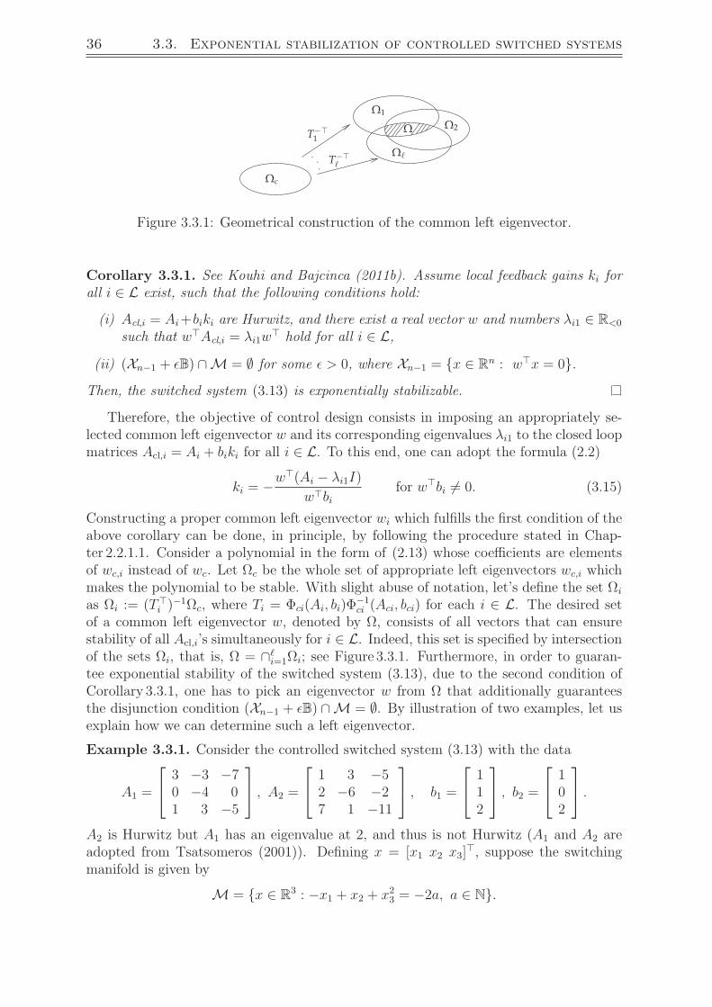
36 3.3. Exponential stabilization of controlled switched systems
Ωc
Ω1
Ω2
ΩT−
T−1
Ω
Figure 3.3.1: Geometrical construction of the common left eigenvector.
Corollary 3.3.1. See Kouhi and Bajcinca (2011b). Assume local feedback gains ki forall i ∈ L exist, such that the following conditions hold:
(i) Acl,i = Ai+biki are Hurwitz, and there exist a real vector w and numbers λi1 ∈ R<0
such that wAcl,i = λi1w hold for all i ∈ L,
(ii) (Xn−1 + εB) ∩M = ∅ for some ε > 0, where Xn−1 = x ∈ Rn : wx = 0.
Then, the switched system (3.13) is exponentially stabilizable.
Therefore, the objective of control design consists in imposing an appropriately se-lected common left eigenvector w and its corresponding eigenvalues λi1 to the closed loopmatrices Acl,i = Ai + biki for all i ∈ L. To this end, one can adopt the formula (2.2)
ki = −w(Ai − λi1I)
wbifor wbi = 0. (3.15)
Constructing a proper common left eigenvector wi which fulfills the first condition of theabove corollary can be done, in principle, by following the procedure stated in Chap-ter 2.2.1.1. Consider a polynomial in the form of (2.13) whose coefficients are elementsof wc,i instead of wc. Let Ωc be the whole set of appropriate left eigenvectors wc,i whichmakes the polynomial to be stable. With slight abuse of notation, let’s define the set Ωi
as Ωi := (Ti )−1Ωc, where Ti = Φci(Ai, bi)Φ
−1ci (Aci, bci) for each i ∈ L. The desired set
of a common left eigenvector w, denoted by Ω, consists of all vectors that can ensurestability of all Acl,i’s simultaneously for i ∈ L. Indeed, this set is specified by intersectionof the sets Ωi, that is, Ω = ∩
i=1Ωi; see Figure 3.3.1. Furthermore, in order to guaran-tee exponential stability of the switched system (3.13), due to the second condition ofCorollary 3.3.1, one has to pick an eigenvector w from Ω that additionally guaranteesthe disjunction condition (Xn−1 + εB) ∩M = ∅. By illustration of two examples, let usexplain how we can determine such a left eigenvector.
Example 3.3.1. Consider the controlled switched system (3.13) with the data
A1 =
⎡⎣ 3 −3 −7
0 −4 01 3 −5
⎤⎦ , A2 =
⎡⎣ 1 3 −5
2 −6 −27 1 −11
⎤⎦ , b1 =
⎡⎣ 1
12
⎤⎦ , b2 =
⎡⎣ 1
02
⎤⎦ .
A2 is Hurwitz but A1 has an eigenvalue at 2, and thus is not Hurwitz (A1 and A2 areadopted from Tsatsomeros (2001)). Defining x = [x1 x2 x3]
, suppose the switchingmanifold is given by
M = x ∈ R3 : −x1 + x2 + x23 = −2a, a ∈ N.
Chapter 3. Switched linear systems with state dependent switching 37
Assume we are interested in designing a control u = kσ(x)x for σ(x) ∈ 1, 2, such thatthe resulting switched system is exponentially stable. Using the transformation z = Tix,with Ti = Φci(Ai, bi)Φ
−1ci (Aci, bci) for i ∈ L := 1, 2, given by
T1 =
−72 −8 1−8 2 1−32 6 2
, T2 =
−4 7 1−8 −2 020 17 2
,the matrices Ai for i ∈ L are converted to control canonical forms; see Chapter 2.2.1.1.Now, let’s denote a desired left eigenvector of the controllable canonical form of the ith
mode by wci = [wci1 wci2 wci3]> for each i ∈ L. For each i ∈ 1, 2, the polynomial
hi(λ) = wci3λ2 + wci2λ+ wci1
is Hurwitz when wc,ij > 0 for j ∈ 1, 2, 3. On the other hand, recall from Chapter 2.2.1.1that the relationship between the left eigenvectors w and wc,i corresponding to the closedloop matrices Acl,i and Ac,cl,i (controllable canonical form of Acl,i), respectively, is givenby w = T−>i wci for each i ∈ L. Therefore, for computing an appropriate common lefteigenvector that stabilizes this switched system, we need to satisfy the following criteria:
T−>1 wc1 − T−>2 wc2 = 0,
wc,ij > 0 ∀ i ∈ 1, 2, j ∈ 1, 2, 3.Define the vector w = [w1 w2 w3]>. To meet the condition (X2 + εB ∩M) = ∅ inaccordance with item (ii) of Corollary 3.3.1, we consider the following restrictions onthe elements of w: w1 + w2 = 0, −2w2 + w3 ≤ 0, w2 ≥ 0, and w3 ≥ 0. Havingthese inequalities in hand, it turns out that the disjoint condition is satisfied. Now, theproblem associated with finding w can be approached by optimization technique. Letus define the vectors w>c = [w>c1 w
>c2], ψ1 = [0 −2 1], ψ2 = [0 −1 0], ψ3 = [0 0 −1],
ν = γ[1 1 1 1 1 1 0 0 0]>, and the matrices
R =
[I3 − I3
1 1 0 0 0 0
][(T>1 )−1 0
0 (T>2 )−1
], S =
−I6
ψ1(T>1 )−1 0 0 0
ψ2(T>1 )−1 0 0 0
ψ3(T>1 )−1 0 0 0
.Then, we introduce the following static optimization problem
minimize ‖wc‖2
subject to
Rwc = 0,
Swc ≤ −ν,for some small γ > 0. Note that the variable ν is added to the problem to rule outcomputation of the zero solution. Now, the optimization problem can be solved by“fmincon” command in the MATLAB optimization toolbox. With γ = 0.01, the resultsof this optimization problem are
wc1 =
0.010.0760.0135
, wc2 =
0.12130.08320.01
, w =
−0.00350.00350.0068
.
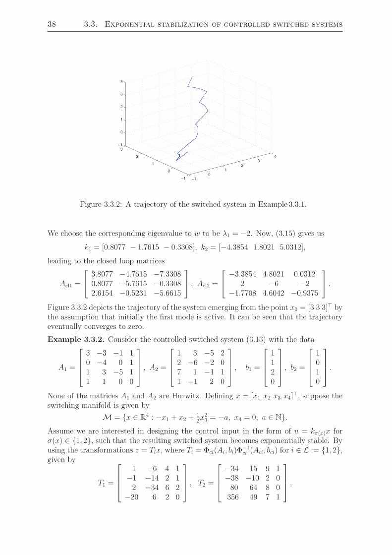
38 3.3. Exponential stabilization of controlled switched systems
−1
0
1
2
3
4
−1
0
1
2
3
−1
0
1
2
3
4
Figure 3.3.2: A trajectory of the switched system in Example 3.3.1.
We choose the corresponding eigenvalue to w to be λ1 = −2. Now, (3.15) gives us
k1 = [0.8077 − 1.7615 − 0.3308], k2 = [−4.3854 1.8021 5.0312],
leading to the closed loop matrices
Acl1 =
⎡⎣ 3.8077 −4.7615 −7.3308
0.8077 −5.7615 −0.33082.6154 −0.5231 −5.6615
⎤⎦ , Acl2 =
⎡⎣ −3.3854 4.8021 0.0312
2 −6 −2−1.7708 4.6042 −0.9375
⎤⎦ .
Figure 3.3.2 depicts the trajectory of the system emerging from the point x0 = [3 3 3] bythe assumption that initially the first mode is active. It can be seen that the trajectoryeventually converges to zero.
Example 3.3.2. Consider the controlled switched system (3.13) with the data
A1 =
⎡⎢⎢⎣
3 −3 −1 10 −4 0 11 3 −5 11 1 0 0
⎤⎥⎥⎦ , A2 =
⎡⎢⎢⎣
1 3 −5 22 −6 −2 07 1 −1 11 −1 2 0
⎤⎥⎥⎦ , b1 =
⎡⎢⎢⎣
1120
⎤⎥⎥⎦ , b2 =
⎡⎢⎢⎣
1010
⎤⎥⎥⎦ .
None of the matrices A1 and A2 are Hurwitz. Defining x = [x1 x2 x3 x4], suppose the
switching manifold is given by
M = x ∈ R4 : −x1 + x2 +
12x23 = −a, x4 = 0, a ∈ N.
Assume we are interested in designing the control input in the form of u = kσ(x)x forσ(x) ∈ 1, 2, such that the resulting switched system becomes exponentially stable. Byusing the transformations z = Tix, where Ti = Φci(Ai, bi)Φ
−1ci (Aci, bci) for i ∈ L := 1, 2,
given by
T1 =
⎡⎢⎢⎣
1 −6 4 1−1 −14 2 12 −34 6 2
−20 6 2 0
⎤⎥⎥⎦ , T2 =
⎡⎢⎢⎣
−34 15 9 1−38 −10 2 080 64 8 0356 49 7 1
⎤⎥⎥⎦ ,

Chapter 3. Switched linear systems with state dependent switching 39
the matrices Ai for i ∈ 1, 2 are converted to controllable canonical forms; see Chap-ter 2.2.1.1. Now, let’s pick a desired left eigenvector of the controllable canonical formwith the following entries: wci = [wci1 wci2 wci3 wci4]> for each i ∈ L. For having thepolynomial
hi(λ) = wci4λ3 + wci3λ
2 + wci2λ+ wci1
to be Hurwitz, we employ Lemma 2.2.2. Sufficient conditions for stability of this poly-nomial are stated by
wc,ij > 0 ∀i ∈ 1, 2, j ∈ 1, 2, 3, 4,wc,i2wc,i3 ≥ 4.0796 wc,i1wc,i4 ∀i ∈ 1, 2.
On the other hand, w = T−>i wci for each i ∈ L is a common left eigenvector of the twosystems, thus
T−>1 wc1 − T−>2 wc2 = 0.
Define w = [w1 w2 w3 w4]>. To satisfy the condition (X2 + εB ∩M) = ∅ in accordancewith item (ii) of Corollary 3.3.1, we impose the following restrictions: w1 + w2 = 0,w2 + w3 ≤ 0, w2 − w3 ≤ 0, and w2 ≥ 0. With these inequalities it turns out thatthe disjoint condition is satisfied. For solving the problem for w, we again employ theoptimization technique. Let us define the vectors w>c = [w>c1 w>c2], ψ1 = [0 1 1 0],ψ2 = [0 1 −1 0], ψ3 = [0 −1 0 0], ν = γ[1 1 1 1 1 1 1 1 0 0 0]>, and the matrices
R =
[I4 − I4
1 1 0 0 0 0 0 0
][(T>1 )−1 0
0 (T>2 )−1
], S =
−I8
ψ1(T>1 )−1 0 0 0 0
ψ2(T>1 )−1 0 0 0 0
ψ3(T>1 )−1 0 0 0 0
.The following static optimization problem now includes all the constraints
minimize ‖wc‖2
subject to
Rwc = 0,
Swc ≤ −ν,−wc,12wc,13 + 4.0796 wc,11wc,14 ≤ 0,
−wc,22wc,23 + 4.0796 wc,21wc,24 ≤ 0.
Note that the vector ν is entered into the problem for excluding computation of zerosolution. Now, the “fmincon” command in the MATLAB optimization toolbox can solvethis optimization problem. The parameters of this optimization problem with γ = 0.01are computed to be
wc1 =
0.00610.00610.04670.0061
, wc2 =
0.75480.58100.12360.0141
, w =
0.0129−0.01290.00310.0013
.

40 3.3. Exponential stabilization of controlled switched systems
One can then choose the eigenvalue associated to w to be λ1 = −2, and then use (3.15)to compute the feedback gains
k1 = [−11.1744 0.3837 3.5930 − 0.9186], k2 = [−2.5202 − 6.4899 2.3283 − 2.2172].
Consequently, the closed loop matrices equal
Acl1 =
−8.1744 −2.6163 2.5930 0.0814
−11.1744 −3.6163 3.5930 0.0814
−21.3488 3.7674 2.1860 −0.8372
1 1 0 0
,
Acl2 =
−1.5202 −3.4899 −2.6717 −0.2172
2 −6 −2 0
7 1 −1 1
−1.5202 −7.4899 4.3283 −2.2172
.Note that Acl1 and Acl2 are both Hurwitz, but no common quadratic Lyapunov functioncan be associated with them. This can be checked by using an appropriate LMI software.
3.3.2 Stabilization of multi-input controlled switched systems
Now, consider a multi-input controlled switched linear system with the switching mani-fold M defined by (3.3), and the system dynamics given by
x = Aσ(x)x(t) +Bσ(x)u(t), (3.16)
where Aσ(x) ∈ Rn×n, Bσ(x) ∈ Rn×m, and
Aσ(x) ∈ A = A1, ..., A`, Bσ(x) ∈ B = B1, ..., B`. (3.17)
The objective of the control design is to exponentially stabilize (3.16) by means of localstate feedbacks u = Kσ(x)x, where Kσ(x) ∈ Rm×n corresponds to the open loop system(Aσ(x), Bσ(x)) for σ(x) ∈ L. For this target, we can again refer to the following corollarywhich is a direct consequence of Theorem 3.2.1.
Corollary 3.3.2. Let Ki for all i ∈ L be local state feedback gains such that
(i) Acl,i = Ai+BiKi are Hurwitz, and there exist a matrix W∈ Rn×(m−1) and a diagonalmatrix Λ = diag([λ1, . . . , λm−1]) with real entries satisfying: W>Acl,i = W>Λ,
(ii) (Xn−m+1 + εB) ∩M = ∅ for some ε > 0, where Xn−m+1 = x ∈ Rn : W>x = 0.Then, the switched system (3.16) is exponentially stabilizable.
We employ the algorithm described in Chapter 2.3 for achieving the criteria of Corol-lary 3.3.2. Namely, we use (m− 1) inputs for assigning an appropriate set of left eigen-vectors given by the columns of W = [w1 . . . wm−1] and their corresponding eigenvaluesgiven by the diagonal entries of Λ = diag([λ1, . . . , λm−1]). In addition, we use a singleinput for assigning the remaining eigenvalues λm, . . . , λn. In summary this algorithmworks as follows:

Chapter 3. Switched linear systems with state dependent switching 41
(i) a set of linearly independent desired left eigenvectors given by the columns ofW = [w1 . . . wm−1] are selected in a manner such that (Xn−m+1 + εB) ∩M = ∅.
(ii) each Ki for i ∈ L splits into two parts, a matrix Ki and a vector kij correspondingto the channels Bi = [bi1 . . . bij−1 bi(j+1) . . . bim] and bij, respectively. The separa-tion is carried out in a way such that ΠiAi has a full set of eigenvectors and thecontrollability matrices Φc(AiΠi, bij) have rank n, where Πi = I−Bi(W
>Bi)−1W>
and det(W>Bi) 6= 0 for all i ∈ L. Note that the index j is not fixed and can bedifferent for each i. Then, we compute the matrix Ai and the vector bi adoptedfrom (2.42) as
Ai =[(I − Bi(W
>Bi)−1W>)Ai + Bi(W
>Bi)−1ΛW>] ,
bi = (I − Bi(W>Bi)
−1W>)bij. (3.18)
(iii) the transformation matrices Ti = [Qi1 Qi2] are acquired from the real Schur de-composition of A>i for all i ∈ L.
(iv) kij is computed by adopting (2.44) and (2.45) for each mode i ∈ L.
(v) Ki is computed by adopting (2.40) for mode i, and the inputs u = Kix anduj = kijx in (2.39) are re-arranged to find the control u = Kix for each i ∈ L.
Now, we provide an example for this algorithm.
Example 3.3.3. Consider a controlled switched system with matrices A1 and A2 asthose in Example 3.3.1 with the switching manifold given by
M = x ∈ R3 : −x1 + x2 + x3 = 2a− 1, a ∈ Z.
The matrices B1 and B2 are
B1 =
1 11 02 2
, B2 =
1 21 01 1
. (3.19)
For stabilization of this switched system, we follow the steps of the above algorithm.By looking at the equation of the switching manifold M, we decide W = [−1 1 1]> tobe the desired common left eigenvector. As (X2 + εB) ∩M = ∅ and det(W>Bi) 6= 0for all i ∈ L and a sufficiently small ε > 0, the requirement of item (i) has alreadybeen fulfilled. For both closed loop matrices Acl1 and Acl2, we choose the closedloop eigenvalues corresponding to W to be λ1 = −2, and the other eigenvaluesto be λ2 = −5 and λ3 = −6. As all the data for the first subsystem is identi-cal to those in Example 2.3.1, we can follow the entire procedure in this example forfinding the appropriate controllers. This gives us k12 = [3 5 −2] and K1 = [0.5 −4.5 −1].
In the second subsystem, we optionally take the first input for partial pole place-ment, whereas the second input is used for assigning the left eigenvector W and itscorresponding eigenvalue λ2. According to this separation, let us define the vectors
42 3.4. Conclusions
b21 = [1 1 1]> and B2 = [2 0 1]>. Define also Π2 similar to Π in (2.46) by signifying theequation with index “2”. As rank Φc(A2Π2, b21) = 3 and Π2A2 has a full set of eigenvec-tors, Lemma 2.3.1 implies that left eigenstructure assignment is possible. Based on thisknowledge, we compute the matrix A2 and the vector b2 in accordance with (2.42)
A2 =
−5 9 1−4 0 4
1 7 −5
, b2 =
312
.Now, computing the real Schur factorization of A>2 defines the matrices Q21, Q22, L21,
and L22 with appropriate dimensions, satisfying Q>21A2 = L21Q>21 and Q>22A2Q22 = L22.
These matrices are numerically computed as
Q>21 =
[0.4082 0.8165 −0.40820.7071 0 0.7071
], L21 =
[−4 0
9.2376 −4
],
Q>22 = [−0.5774 0.5774 0.5774], L22 = −2.
Now, we use (2.44) and (2.45) to compute the appropriate state feedback for this mode,leading to the gain k22 = [−0.9167 −1.5833 0.6667]. Finally, as W>B2 6= 0, we employ(2.40) to obtain K2, yielding the gain K2 = [−6.9167 4.4167 6.6667]. Consequently,the closed loop matrices of the both subsystems equal
Acl1 =
6.5 −2.5 −100.5 −8.5 −18 4 −11
, Acl2 =
−7.75 4.25 3−4.9167 −1.5833 4.6667−0.8333 3.8333 −3.6667
.3.4 Conclusions
In this chapter, we proposed sufficient conditions for stabilization of a class of single- andmulti-input controlled switched linear systems under state dependent switching rules.In this class, the switching signal is specified by a given manifold in the state space.Our proposed approach investigates local state feedback design for each subsystem.The left eigenvectors and eigenstructure assignment techniques for LTI systems are thekey tools for the design. On this basis, we showed that if all closed loop matrices of acontrolled switched linear system share a number of left eigenvectors, then all solutionsof the switched system converge to a known invariant subspace. The idea then lies inthe appropriate selection of the desired common left eigenvectors to ensure Hurwitzstability of the closed loop matrices, and to avoid the situation that the commoninvariant subspace and the switching manifold intersect. Apparently, the structure ofthe switching manifold enforces a significant restriction in this technique. Thus, theproblem of selecting the desired common eigenvectors may include a lot of constraintsespecially when the switching manifold has a complicated topology.

Chapter 4. Switched linear systems with arbitrary switching signals 43
Chapter 4
Switched linear systems witharbitrary switching signals
4.1 Introduction
Despite many interesting results, the stability problem for switched linear systems witharbitrary time-dependent switching signals still remains a challenging research topic.Similar to stability theory for nonlinear systems, Lyapunov’s second theorem is theessential tool for dealing with this problem. It turns out that if there exists a positivedefinite function which decreases in time along the system solutions, then the switchedlinear system is exponentially stable (Shorten et al., 2007). Such a function is calleda common Lyapunov function for the switched system. When the common Lyapunovfunction is quadratic and satisfies separately the Lyapunov function properties for allmodes, it is called a common quadratic Lyapunov function (CQLF), and the switchedsystem is called quadratically stable. It is known that quadratic stability of a switchedsystem implies its exponential stability, and we will also give a short proof for thisfact in this chapter. As a matter of fact, referring to the converse Lyapunov theorem,exponential stability for a switched linear system is equivalent to the existence of acommon Lyapunov function for such system; see Shorten et al. (2007) and the referencestherein.
In this chapter, we study quadratic stability and stabilization (see Problems 1.3.1,and 1.4.1) of several classes of switched linear systems. We show that if all constituentmatrices of a switched linear system are individually Hurwitz and share an (n − m)dimensional right invariant subspace to which a common quadratic Lyapunov functioncan be associated, and if a set of m common left eigenvectors perpendicular to thisinvariant subspace exists, then the switched linear system is quadratically stable.One direct consequence of this result is quadratic stability of switched systems whoseconstituent matrices have (n − 1) common right eigenvectors (Shorten and Cairbre,2001), or (n− 1) common real left eigenvectors (Kouhi and Bajcinca, 2011b). Moreover,we discuss robust stability of switched linear systems, particularly for systems with(n− 1) common real left eigenvectors.
In addition, we propose the notion of block similarity for controlled switched linear

44 4.2. Quadratic stability of switched linear systems
systems, and demonstrate that the quadratic stability problem for block similar matricesis equivalent. This result may particularly be applicable for controlled switched systemswhere the closed loop matrices can be transformed to block triangular form. Then,we identify one such class, namely the class of controlled switched systems where theopen loop matrices share an invariant subspace with appropriate dimension to which acommon quadratic Lyapunov function can be associated. For this class, we utilize the lefteigenvectors assignment approach to design local feedbacks which make the controlledswitched systems quadratically stable. This result extends parts of the results by Kouhiand Bajcinca (2011c), where (n− 1) inputs are assumed for stabilization of a controlledswitched linear system. We develop further this approach for stabilization of a controlledswitched system whose open loop matrices own (n−m) dimensional invariant subspaceswhich are sufficiently close, and all matrices associated with the invariant subspacessatisfy a certain form of Riccati inequalities instead of Lyapunov inequalities.
4.2 Quadratic stability of switched linear systems
We study quadratic stability of switched linear systems under arbitrary time-dependentswitching signals. Our switched linear system is defined as
x = Aσ(t)x(t) Aσ(t) ∈ A := A1, . . . , A`, (4.1)
where x(t0) = x0 ∈ Rn and σ : R≥0 → L := 1, . . . , ` is a piecewise constant functionreferred to as the switching signal between different modes, that is, x = Aix(t) for i ∈ L.Note that the only restriction on the switching is that a finite number of switching occurswithin each finite time interval. Given an initial condition x0, the Caratheodory solution(see Appendix A.6.2.1) of the switched system (4.1) is unique and is given by
x(t) = eAσk (t−tk) . . . eAσ0 (t1−t0)x0, (4.2)
where tk > · · · > t2 > t1 are the switching time instances, t > tk, t1 > t0, and σj := σ(tj)for all j ∈ 0, . . . , k; see (Shorten et al., 2007). The uniqueness of the solution resultsfrom the fact that at each time instance only one subsystem is active, and for any activemode i ∈ L the vector field fi := Aix is locally Lipschitz. It is known that differentialequations with locally Lipschitz vector fields possess unique solutions (Coddington andLevinson, 1955; Cortes, 2008).
Recall from Problem 1.3.1 that the switched linear system (4.1) is called quadraticallystable if and only if there exists a function V (x) = x>Px with P symmetric positivedefinite, such that
A>i P + PAi < 0 ∀Ai ∈ A. (4.3)
Now, we attempt to prove that quadratic stability of switched linear systems impliestheir exponential stability, a fact which was already explored and existed in the literature(Shorten et al., 2007). To see this, assume that all matrices Ai for i ∈ L share a quadraticLyapunov function V (x) = x>Px. As A>i P + PAi < 0 for all i ∈ L, then there exists anumber γ > 0, such that
A>i P+PAi < −γI⇒ V (x) = x>(A>i P + PAi)x ≤ −γ‖x‖2.

Chapter 4. Switched linear systems with arbitrary switching signals 45
On the other hand, as P is symmetric positive definite, the following inequalities arevalid
λmin(P )‖x‖2 ≤ x>Px = V (x) ≤ λmax(P )‖x‖2. (4.4)
Therefore,
V (x) =x>(A>i P + PAi)x ≤ −γ‖x‖2 ≤ −γλmax(P )
V (x)
⇒ V (x) ≤ V (x0)e−β(t−t0),
where β := γ/λmax(P ). Now, paying attention to (4.4), we can deduce
λmin(P )‖x‖2 ≤ V (x) ≤ V (x0)e−β(t−t0) ⇒ ‖x‖2 ≤ V (x0)
λmin(P )e−β(t−t0).
This implies exponential stability of the switched linear system (4.1). Therefore, numer-ous contributions offering sufficient conditions for the existence of a common Lyapunovsolution for a set of Hurwitz matrices have appeared in the literature, including Shortenand Narendra (1998); Narendra and Balakrishnan (1994); Shorten and Cairbre (2001).One of the established results in this context concerns this problem for a set of similarmatrices. The following lemma points out this result in detail.
Lemma 4.2.1. (See also Wulff (2005); Shorten et al. (2007)) Suppose in the switchedlinear system (4.1), each Ai ∈ Rn×n is block similar to Ai ∈ Cn×n for i ∈ L, obtained by asimilarity transformation matrix S ∈ Cn×n. Then, there exists a real common Lyapunovsolution P = P> > 0 for all Ai, if and only if there exists a Hermitian common Lyapunovsolution P = P ∗ > 0 for all Ai, that is, A∗i P + P Ai < 0 for all i ∈ L.
Proof of sufficiency: As Ai is block similar to Ai for all i ∈ L by using a similaritytransformation S ∈ Cn×n, one can write
Ai = S−1AiS; (4.5)
see Appendix A.2.12. Now, suppose there exists a positive definite matrix P = P> suchthat A>i P + PAi < 0. By pre-multiplying this inequality by S∗ and post-multiplying itby S, the sign of the inequality does not change. Therefore, we have
S∗A>i PS + S∗PAiS < 0⇒ A∗i P + P Ai < 0 ∀i ∈ L,
where P = S∗PS > 0 is Hermitian.
Proof of necessity: Suppose there exists a Hermitian P > 0 such that A∗i P + P Ai < 0.Then, by pre-multiplying this inequality by S−∗ and post-multiplying it by S−1, the signof this inequality does not change. Hence, we can write
S−∗A∗i PS−1 + S−∗P AiS
−1 < 0⇒ A>i (S−∗PS−1) + (S−∗PS−1)Ai < 0 ∀i ∈ L.

46 4.2. Quadratic stability of switched linear systems
Now, define P = Re (S−∗PS−1), and consider the function V (x) = x>Px for x ∈ Rn.We show V (x) is indeed a CQLF for the switched linear system (4.1). As S−∗PS−1 isHermitian, P is symmetric. Moreover, for x ∈ Rn\0 we have
V (x) = x>Px = x>S−∗PS−1x > 0,
V (x) = x>(A>i P + PAi)x = x>(S−∗A∗i PS−1 + S−∗P AiS
−1)x < 0.
The first inequality implies that P > 0, and the second inequality implies that V (x) isdecreasing along the solutions of the switched system. Hence, V (x) satisfies the criteriaof a CQLF.
In the sequel, we aim at establishing conditions on the Ai’s, such that these matricesshare a Lyapunov solution. Our approaches rely on the concept of common eigenvectorsand invariant subspaces. To gain more intuition about our approach, we outline thefollowing principle. Consider the special case that all Hurwitz matrices in the switchedlinear system (4.1) share a set of m linearly independent left eigenvectors given by thecolumns of W = [w1 . . . wm] ∈ Cn×m corresponding to a set of eigenvalues given by thediagonal elements of the matrix Λi = diag([λi1, . . . , λim]) for each i ∈ L. Notice when wjfor j ∈ 1, . . . ,m is a left eigenvector of Ai corresponding to the eigenvalue λij, thenwj is also a left eigenvector of the matrix eAit corresponding to the eigenvalue eλijt. Thisfact can be proved via exploiting the Taylor expansion of eAit
eAit = I + Ait+(Ait)
2
2!+ · · · . (4.6)
Then, by pre-multiplication of (4.6) by W ∗ and considering the identity W ∗Ai = ΛiW∗,
we will have
W ∗eAit =
(I + Λit+
(Λit)2
2!+ · · ·
)W ∗ = eΛitW ∗.
Further, pre-multiplying (4.2) by W ∗, the following property holds
W ∗x(t) = eΛσk (t−tk)eΛσk−1(tk−tk−1) . . . eΛσ0 (t1−t0)W ∗x0.
Suppose all eigenvalues λij for i ∈ L and j ∈ 1, . . . ,m have negative real parts, thatis, Re (λij) < 0. Assuming λ0 = max (Re(λij)) for i ∈ L and j ∈ 1, . . . ,m, we canwrite
‖W ∗x(t)‖ =‖eΛσk (t−tk)eΛσk−1(tk−tk−1) . . . eΛσ0 (t1−t0)W ∗x0‖
≤ ‖eΛσk (t−tk)‖.‖eΛσk−1(tk−tk−1)‖ . . . ‖eΛσ0 (t1−t0)‖.‖W ∗x0‖
≤ eλ0(t−tk).eλ0(tk−tk−1) . . . eλ0(t1−t0)‖W ∗x0‖ = eλ0(t−t0)‖W ∗x0‖.This means that all solutions (4.2) converge exponentially to a set defined by
Xn−m = x ∈ Cn : W ∗x = 0, (4.7)
in the worst case with time constant −1/λ0. On the other hand, the following property
x ∈ Xn−m ⇒ W ∗x = W ∗Aix = ΛiW∗x = 0 ∀i ∈ L
indicates that the set Xn−m is invariant for the switched system (4.1).
We consider this principle as the initial step for developing our results in this chapter;see also Kouhi and Bajcinca (2011b).

Chapter 4. Switched linear systems with arbitrary switching signals 47
4.2.1 Stability of switched systems with a common invariantsubspace
Motivated by the previous discussion, we now assume that all matrices in the switchedsystem (4.1) are Hurwitz and share m linearly independent left eigenvectors correspond-ing to m eigenvalues with negative real parts. We explored that the solution startingfrom an initial point x0 outside of Xn−m, defined by (4.7), exponentially converges to thisset. Now, as our switched system consists of linear flows, we hope quadratic stability ofthe system inside the invariant subspace can imply quadratic stability of the switchedsystem in the entire state space. The correctness of this conjecture is established byaccomplishing the proof of the next theorem.
Theorem 4.2.1. Consider the switched linear system defined by (4.1). Let all Ai ∈ Abe Hurwitz, and share m linearly independent left eigenvectors given by the columns ofW = [w1 . . . wm] corresponding to the eigenvalues given by the diagonal entries of thematrices Λi = diag([λi1, . . . , λim]) for all i ∈ L. Furthermore, suppose the columns ofV ∈ Cn×(n−m) are an orthonormal basis for the common invariant subspace of all Ai ∈ A,namely Xn−m ⊂ Cn defined by (4.7), corresponding to the eigenvalues λi,m+1, . . . , λi,n fori ∈ L, that is,
AiV = V Li, and W ∗V = 0, (4.8)
where Li ∈ C(n−m)×(n−m) for all i ∈ L. Moreover, assume that the systems ˙x = Lixshare a CQLF, that is, there exist a function V(x) = x∗Px with P ∈ C(n−m)×(n−m) andP = P∗ > 0, such that the following Lyapunov inequalities hold
L∗iP + PLi < 0 ∀ i ∈ L. (4.9)
Then, the switched linear system (4.1) is quadratically stable.
Proof: Let us define the reduced QR-factorization of W as
W = Q1R1, (4.10)
where R1 is an m×m upper triangular non-singular matrix and Q1 is an n×m matrixwhich has orthonormal columns, that is, Q∗1Q = Im; see Appendix A.2.8. As the columnsof W contain the set of left eigenvectors of Ai, we can write
W ∗Ai = ΛiW∗ ⇒ R∗1Q
∗1Ai = ΛiR
∗1Q∗1 ⇒ Q∗1AiQ1 = R−∗1 ΛiR
∗1.
Since Λi is diagonal and its main diagonal elements have negative real parts, Im is acommon Lyapunov solution for the Λi’s for all i ∈ L. Then, referring to Lemma 4.2.1,R−∗1 ΛiR
∗1 also share a Lyapunov solution in the form of P1 = R1R
∗1 for all i ∈ L. On the
other hand, it follows from
W ∗V = 0⇒ R∗1Q∗1V = 0⇒ Q∗1V = 0, (4.11)

48 4.2. Quadratic stability of switched linear systems
that the matrix T = [Q1 V ] is an orthonormal matrix, i.e., T ∗T = In. Considering thetransformed matrices Ai := T ∗AiT , each Ai ∈ A is similar to
Ai =
[R−∗1 ΛiR
∗1 0
Xi Li
],
where Xi := V ∗AiQ1 ∈ C(n−m)×m. It is inferred from Lemma 4.2.1 that Ai share aLyapunov solution if and only if Ai share a Lyapunov solution for all i ∈ L. Next, weshow that Ai share a Lyapunov solution in the form of
P = 12
[R1R
∗1 0
0 εP
], (4.12)
where P satisfies the inequality (4.9) and ε > 0 is a scalar which must be properlyselected. In fact, we have
A∗i P + P Ai =
[R1Re(Λi)R
∗1
ε2X∗i P
ε2PXi
ε2(PLi + L∗iP)
]. (4.13)
Note that R1Re(Λi)R∗1 < 0 because all Ai ∈ A are individually Hurwitz. Thus, the
matrix in (4.13) is negative definite if and only if its Schur complement with respect tothe upper left block, denoted by Si, is negative definite; see Appendix A.2.2. The Schurcomplement,
Si = ε2(PLi + L∗iP)− ε2
4PXi [R1Re(Λi)R
∗1]−1X∗i P ∀i ∈ L, (4.14)
is negative definite for small ε, for instance with
ε = mini∈L
(λmax(PLi + L∗iP)
λmin(PXi [R1Re(Λi)R∗1]−1X∗i P)
). (4.15)
Thus, referring to Lemma 4.2.1 the existence of a common Lyapunov solution for Ai ∈ Ais guaranteed if we pick P = P> = Re(T PT ∗). Now, substituting P from (4.12), we get
T PT ∗ = 12
[Q1 V ]
[R1R
∗1 0
0 εP
] [Q∗1V ∗
]= 1
2(WW ∗ + εV PV ∗) .
This means that the Lyapunov function has the form V (x) = x>Px, where
P = 12
Re (WW ∗ + εV PV ∗) . (4.16)
A different statement and proof of Theorem 4.2.1 has been presented in Bajcinca et al.(2013).
4.2.1.1 Stability with (n− 1) common right eigenvectors
Now, consider that all matrices Ai ∈ A in the switched system (4.1) are Hurwitz andshare (n − 1) linearly independent right eigenvectors given by the columns of V =
Chapter 4. Switched linear systems with arbitrary switching signals 49
[v1 . . . vn−1] ∈ Cn×(n−1) corresponding to (n−1) eigenvalues given by the diagonal entriesof Λi = diag([λi2, . . . , λin]), satisfying
AiV = V Λi ∀i ∈ L. (4.17)
Then, they share a left eigenvector w corresponding to the eigenvalues λi1 withRe(λi1)< 0 for all i ∈ L, satisfying the property
w∗V = 0.
Let us define the reduced QR-factorization of V as
V = Q2R2,
where R2 ∈ C(n−1)×(n−1) is an upper triangular non-singular matrix and Q2 ∈ Cn×(n−1)
has orthonormal columns, that is, Q∗2Q2 = In−1. As the columns of V contain a set ofeigenvectors of Ai ∈ A, we have
AiV = V Λi ⇒ AiQ2R2 = Q2R2Λi ⇒ AiQ2 = Q2(R2ΛiR−12 ).
Note again that Λi to be diagonal with the entries located in the open left half planeimplies that In−1 is a common Lyapunov solution for Λi for each i ∈ L. Then, referringto Lemma 4.2.1, R2ΛiR
−12 also share a Lyapunov solution in the form of P = R−∗2 R−1
2 forall i ∈ L. Therefore, referring to Theorem 4.2.1, the switched system (4.1) has a CQLFin the form of V (x) = x>Px with
P = 12
Re(ww∗ + εQ2 R
−∗2 R−1
2 Q∗2)
=
= 12
Re(ww∗ + εV
[R−1
2 R−∗2 R−12 R−∗2
]V ∗), (4.18)
where ε is a scalar which can be computed with regard to (4.15).
Quadratic stability of a switched linear system when all its constituent matrices areHurwitz and share (n− 1) right eigenvectors has been previously shown by Shorten andCairbre (2001).
4.2.1.2 Stability with (n− 1) common real left eigenvectors
Now, consider that all Ai’s in the switched system (4.1) share (n−1) linearly independentleft eigenvectors wj ∈ Rn for all j ∈ 1, . . . , n−1 corresponding to the (n−1) eigenvaluesλi1, . . . , λi(n−1) for i ∈ L. Then, they share a right eigenvector vn corresponding to then-th eigenvalues λin for all i ∈ L, satisfying the property
w>j vn = 0 ∀j ∈ 1, . . . , n− 1.
Now we plan to compute the analytical expression of the solutions of switched system(4.1) given in (4.2) with respect to its eigenvalues and eigenvectors; see also Kouhi andBajcinca (2011c). To this end, consider the eigenvalue decomposition
Ai = ViΛiW>i ∀i ∈ L, (4.19)
where Λi = diag([λi1, . . . , λin]), Vi = [vi1 . . . vi(n−1) vn], and Wi = [w1 . . . wn−1 win].We also assume that Vi and Wi have normal columns. Referring to our discussion in

50 4.2. Quadratic stability of switched linear systems
Section 4.2, the diagonal entries of eΛσj are eigenvalues of eAσj for any j ∈ 0, . . . , k.Thus, we can write
eAσj (tj+1−tj) = VσjeΛσj (tj+1−tj)W>
σj,
where by definition of eigenvectors, the following relationships must hold
w>r vσjs = 0, w>r vσjr = 1, w>r vn = 0, w>σjnvn = 1 ∀r, s ∈ 1, . . . , n− 1, r 6= s.
Then, we have
W>σjVσj−1
=
w>1...
w>n−1
w>σjn
[ vσj−11 . . . vσj−1(n−1) vn]
=
1 0 . . . 0 00 1 . . . 0 0...0 0 . . . 1 0
w>σjnvσj−11 w>σjnvσj−12 . . . w>σjnvσj−1(n−1) 1
.
Defining θjq := λσjq(tj+1 − tj) for each q ∈ 1, . . . , n to simplify the notation, a part ofthe expression (4.2) is computed as follows:
eAσj (tj+1−tj)eAσj−1 (tj−tj−1) =(Vσje
Λσj (tj+1−tj)W>σj
)(Vσj−1
eΛσj−1 (tj−tj−1)W>σj−1
)= (4.20)
= Vσj
eθj1 0 . . . 0 00 eθj2 . . . 0 0...0 0 . . . eθj(n−1) 00 0 . . . 0 eθjn
1 0 . . . 0 00 1 . . . 0 0...0 0 . . . 1 0
w>σjnvσj−11 w>σjnvσj−12 . . . w>σjnvσj−1(n−1) 1
×
eθ(j−1)1 0 . . . 0 0
0 eθ(j−1)2 . . . 0 0...
...0 0 . . . eθ(j−1)(n−1) 00 0 . . . 0 eθ(j−1)n
W>σj−1
= Vσj
eθj1+θ(j−1)1 . . . 0 0
...0 . . . eθj(n−1)+θ(j−1)(n−1) 0
eθjn+θ(j−1)1w>σjnvσj−11 . . . eθjn+θ(j−1)(n−1)w>σjnvσj−1(n−1) eθjn+θ(j−1)n
W>σj−1
.

Chapter 4. Switched linear systems with arbitrary switching signals 51
Note that for consistency of notation, we assume tk+1 := t. Now, referring to (4.2) and(4.19) the analytical solution of the switched linear system (4.1) equals
x(t) =(Vσke
Λσk (t−tk)W>σk
)(Vσk−1
eΛσk−1(tk−tk−1)W>
σk−1
). . .(Vσ0e
Λσ0 (t1−t0)W>σ0
)x0
= Vσk
(eΛσk (t−tk)W>
σkVσk−1
eΛσk−1(tk−tk−1)W>
σk−1. . . Vσ0e
Λσ0 (t1−t0)) (W>σ0x0
). (4.21)
Now, recalling (4.20), and considering the following computation
U : = eΛσk (t−tk)W>σkVσk−1
eΛσk−1(tk−tk−1)W>
σk−1· · ·Vσ0eΛσ0 (t1−t0)
=
eθk1+···+θ01 0 . . . 0
...0 . . . eθk(n−1)+···+θ0(n−1) 0
κ1(t) . . . κn−1(t) eθkn+···+θ0n
,where
κr(t) =k∑p=1
eθkn+···+θ(k−p+1)n+θ(k−p)r+···+θ0r(w>σk−p+1nvσk−pr) ∀r ∈ 1, . . . , n− 1,
the analytical solution (4.21) reads
x(t) =[vσk1 . . . vσk(n−1) vn
]U
w>1 x0
...w>n−1x0
w>σ0nx0
.This leads to the more explicit form of the solution, given by
x(t) =n−1∑r=1
(w>r x0) eθkr+···+θ0r vσkr+
+
(n−1∑r=1
(w>r x0)κr(t) + eθkn+···+θ0n(w>σ0nx0
))vn. (4.22)
The expression (4.22) reveals that the shape of the solution is determined by the righteigenvectors of the k-th switching mode, while the speed of the solution is governed bythe eigenvalues of all switching modes. Further, we show that when all Ai are Hurwitz,the solution x(t) eventually converges exponentially to zero. Defining
λ0 = maxi∈L
λ(Ai), ∆t = minj∈0,...,k−1
(tj+1 − tj),
where k ∈ N, and considering that all eigenvalues of Ai ∈ A are real negative, and thefact that ∆t > 0, we can derive the following upper bound for κr(t)
κr(t) ≤ eλ0(k∆t+(t−tk))
k∑j=1
w>σk−j+1nvσk−jr ≤ eλ0(k∆t+(t−tk))k ∀r ∈ 1, . . . , n− 1.

52 4.2. Quadratic stability of switched linear systems
Define t = k∆t+ (t− tk), and notice t→∞ if and only if t→∞ . As limt→∞ eλ0 tk = 0,we must have
limt→∞
kr(t) = 0 ∀r ∈ 1, . . . , n− 1.This implies that the solution (4.22) converges exponentially to zero if all matrices Ai ∈ Aare Hurwitz, that is,
limt→∞
x(t) = 0.
The proof of exponential stability for this switched linear system can alternatively beachieved, by the result of Theorem 4.2.1. Note that a switched linear system with(n − 1) real common left eigenvectors share basically a real right eigenvector whichdefines a common invariant subspace with dimension 1. Then, it immediately followsfrom Theorem 4.2.1 that the switched system (4.1) is quadratically stable.
Now, we compute a CQLF for this class of switched linear systems. We follow theproof of Theorem 4.2.1. Let us denote the normal real common eigenvector of Ai ∈ Acorresponding to λin by vn, and the reduced QR-factorization of W := [w1 . . . wn−1] asW = Q1R1, where R1 ∈ R(n−1)×(n−1) is invertible and Q1 ∈ Rn×(n−1) has orthonormalcolumns. Now, notice in this case, for using Theorem 4.2.1 we should assume Li = λin,V = vn, and Λi = diag([λi1, . . . , λi(n−1)]). Let us define the orthonormal transformationmatrix T = [Q1 vn] and the transformed matrices Ai := T>AiT for i ∈ L. By definition,each Ai is similar to
Ai =
[R−>1 ΛiR
>1 0
v>nAiQ1 λin
].
Next, we argue that Ai share a Lyapunov solution in the form of
P = 12
[R1R
>1 0
0 ε
], (4.23)
where ε > 0 is a scalar. To this end, the Lyapunov equation for each Ai equals:
A>i P + P Ai =
[R1ΛiR
>1
ε2
(v>nAiQ1
)>ε2v>nAiQ1 ελin
]. (4.24)
The Schur complement of (4.24) with respect to the block R1ΛiR>1 reads:
Si = ελin − ε2
4(v>nAiQ1)(R1ΛiR
>1 )−1(v>nAiQ1)> ∀i ∈ L.
Obviously, Si is negative definite for small ε. For instance, with regard to (4.15) we canselect
ε = mini∈L
(2λin
(v>nAiQ1)(R1ΛiR>1 )−1(v>nAiQ1)>
).
Thus, referring to Lemma 4.2.1, we can choose a CQLF as V (x) = x>Px with P = P> =T PT>. Now, substituting P from (4.23), we get
P = T PT> = 12
[Q1 vn]
[R1R
>1 0
0 ε
][Q>1
v>n
]= 1
2(WW> + εvnv
>n ).

Chapter 4. Switched linear systems with arbitrary switching signals 53
This means that the Lyapunov function has the form
V (x) = 12x>(WW> + εvnv
>n
)x = 1
2
n−1∑i=1
(w>i x)2 + 12ε(v>n x)2. (4.25)
This Lyapunov function is consistent with the one introduced in (Kouhi and Bajcinca,2011c) which was derived by using a different approach. The particular case when thedimensions of Ai are two, that is, n = 2, has been already studied in Example 3.2.3.
4.3 Robust Stability of switched linear systems
Consider again the switched linear system (4.1). This system features a discontinuousvector field f : R≥0 × Rn → Rn in the form of
x = Aσ(t)x =: f(t, x).
Such differential equations can be approximated by a convexified differential inclusion
ΣF : x ∈ F (x) := co Ax : A ∈ A =∑i=1
γi Aix, (4.26)
where ∑i=1
γi = 1, γi ≥ 0 ∀i ∈ L,
and co stands for the convex hull (Kouhi and Bajcinca, 2011c; Shorten et al., 2007).Then, the solution (4.2) is contained in the set of Caratheodory solutions of the lineardifferential inclusions (4.26). The set-valued map F (x) in (4.26) satisfies the so called“basic conditions” as it is outer semi-continuous on Rn, and at any x ∈ Rn, F (x) iscompact and convex; see Teel and Praly (2000) and Appendix A.7. Now, we introducethe notion of robust stability for switched linear system (4.1) based on the definition ofrobust stability for differential inclusion (4.26).
Definition 4.3.1. (Teel and Praly, 2000; Cai et al., 2007; Clarke et al., 1997), A smoothfunction V (x) is a robust Lyapunov function for the differential inclusion (4.26) if thereexist two increasing positive definite functions α1, α2 : [0,∞)→ [0,∞) satisfying
α1(‖x‖) ≤ V (x) ≤ α2(‖x‖), (4.27)
maxf∈F (x)
〈∇V (x), f〉 ≤ −V (x). (4.28)
Definition 4.3.2. (Teel and Praly, 2000) The differential inclusion x ∈ F (x) is said tobe robustly asymptotically stable if a continuous perturbation function δ : Rn → R≥0
with δ(x) > 0 for x ∈ Rn\0 exists, such that the perturbed differential inclusion
x ∈ Fδ(x)(x) := co F (x+ δ(x)B) + δ(x)B (4.29)
is asymptotically stable, where B denotes the closed unit ball in Rn.

54 4.3. Robust Stability of switched linear systems
In Teel and Praly (2000) it has been shown that, in general, robust asymptoticstability of a differential inclusion with F satisfying the basic conditions is equivalentto the existence of a robust Lyapunov function. Specifically, it turns out that theexistence of a robust Lyapunov function is a sufficient and necessary condition forrobust exponential stability of (4.26); see also Appendix A.7.1.
Now, we aim at establishing conditions under which quadratic stability of a switchedlinear system implies its robust stability in the sense of Definition 4.3.1 and Defini-tion 4.3.2. Let us assume a CQLF, V (x) = x>Px with P = P> > 0, for the switchedsystem (4.1) exists such that the condition (4.28) also holds. This means
A>i P + PAi + P ≤ 0,
or, equivalently (Ai + 1
2I)>P + P
(Ai + 1
2I)≤ 0 ∀i ∈ L. (4.30)
This implies that all matrices Ai + 12I share a weak Lyapunov solution. Furthermore,
we claim that (4.30) is sufficient for robust stability of the differential inclusion (4.26),and the condition (4.27) automatically holds when the Lyapunov function is quadratic.Indeed, for the CQLF V (x) = x>Px, convenient functions α1 and α2 are
α1(‖x‖) = λmin(P )‖x‖2, α2(‖x‖) = λmax(P )‖x‖2. (4.31)
Then, from the results by Teel and Praly (2000), the differential inclusion (4.26) isrobustly exponentially stable, provided that (4.30) holds.
Although the result by Teel and Praly (2000) provides simple criteria for robuststability of differential inclusion (4.26), the perturbation bound δ, introduced by Def-inition 4.3.2, will be characterized by the eigenvalues of P . Although many articlesconcerning the computations of upper and lower bounds for eigenvalues of a Lyapunovmatrix P exists in the literature, this problem still undergoes more research (Lee, 1997).That means we are not able to describe δ explicitly by the system parameters. Thus,we do not involve ourselves for computing such a perturbation function in the generalcase. Alternatively, we consider a special case of switched systems, where all constituentsAi ∈ A share (n− 1) real left eigenvectors. For such a system, the structure of the Lya-punov function allows us to find a perturbation bound δ(x) which is only represented bythe system parameters.
4.3.1 Robust stability with (n−1) common real left eigenvectors
We have shown so far, that the switched system (4.1) is quadratically stable if all matricesAi ∈ A are Hurwitz and share (n − 1) real left eigenvectors. In this part, we wishto establish conditions under which this class of switched linear systems is robustlyexponentially stable. The next theorem illustrates this result.
Theorem 4.3.1. (Kouhi and Bajcinca, 2011c) Consider the switched system (4.1). Letall Ai ∈ A be Hurwitz, and share (n− 1) real linearly independent left eigenvectors given
Chapter 4. Switched linear systems with arbitrary switching signals 55
by the columns of W = [w1 . . . wn−1], such that w>j wj = 1 for all j ∈ 1, . . . , n − 1.Then, for a continuous perturbation function δ : Rn → R≥0, the convexified linear differ-ential inclusion represented by (4.26) is robustly exponentially stable if the eigenvaluesof Ai satisfy: λij < −1
2for all i ∈ L and j ∈ 1, . . . , n.
Proof: In Section 4.2.1.2 we showed that for a sufficiently small ε, V (x) = x>Px withP = 1
2WW> + 1
2εvnv
>n is a CQLF for the switched linear system (4.1). In other words,
the inequalities A>i P + PAi < 0 hold for all i ∈ L. Employing the same structure ofP , we need again to show that an ε exists, such that the differential inclusion (4.26) isexponentially stable. To this end, we can basically follow the same lines of the previousarguments, by taking into account that
λ(Ai + 1
2I)
= λ(Ai) + 12, (4.32)
and the eigenvectors of Ai and Ai + 12I are equal. Consequently, it turns out that by
referring to (4.15) and choosing
ε < mini∈L
(2(λin + 1
2)
(v>nAiQ1)(R1(Λi + 12In−1)R>1 )−1(v>nAiQ1)>
), (4.33)
V (x) is a robust Lyapunov function for the differential inclusion (4.26).
Note that P = 12WW>+ 1
2εvnv
>n has one eigenvalue equal 1
2ε and its other eigenvalues
are eigenvalues of 12W>W . This can be verified by observing that
P vn = 12εvn,
P W = W (12W>W ).
The first relationship implies that vn is the eigenvector of P corresponding to the eigen-value 1
2ε, and the second one implies that P has an (n − 1) dimensional right invariant
subspace with columns of W as its basis. Thus, it follows from this relation that (n− 1)eigenvalues of P are embedded in 1
2W>W . As W has normalized columns and ε can be
choose sufficiently small, we can write
λmin(P ) = 12ε, and λmax(P ) ≤ tr (1
2W>W ) = 1
2(n− 1); (4.34)
see also Appendix A.2.11. Now, we propose an upper bound for the uncertainty functionδ(x) such that despite its presence exponential stability of the perturbed differentialinclusion defined by (4.29) is ensured. Let’s denote the maximum singular value of Aiby σmax(Ai) and introduce Lipschitz functions δi(x) for all i ∈ L as
δi(x) = ψi.‖x‖, where ψi :=ε
4(n− 1)(σmax(Ai) + 1). (4.35)
We then choose the function δ(x) in (4.29) as
δ(x) = ψ.‖x‖, where ψ = min ψ1, . . . , ψ` . (4.36)

56 4.4. Quadratic stabilization of switched linear systems
The perturbed set valued map defined in (4.29) equals
Fδ(x)(x) =
∑i=1
γiAix+ ψ.‖x‖((∑
i=1
.γiAi
)+ I
)B
,∑i=1
γi = 1, γi ≥ 0 ∀i ∈ L.
Considering (4.34), (4.30), and the definition of ψi in (4.35), for x 6= 0 we have
maxf∈Fδ(x)
〈∇V (x), f〉 = maxf∈Fδ(x)
〈2x>P, f〉
= maxv∈B
(∑i=1
(γix>(A>i P + PAi)x
)+ 2
∑i=1
(γi.ψ.‖x‖.x>P.(Ai + I)v
))
≤ −x>Px+ 2 maxv∈B
(∑i=1
(γiψi.‖x‖.‖x>P‖.‖(Ai + I)v‖
))
≤ −x>Px+ 2∑i=1
(γiψi.‖x‖.λmax(P ).‖x‖. (σmax(Ai) + 1))
≤ −x>Px+1
4ε.‖x‖.‖x‖
≤ −1
2x>Px < 0. (4.37)
Furthermore, it follows from (4.37) that
V (x) ≤ −12x>Px = −1
2V (x)⇒ V (x) ≤ V (x0)e−
12t.
Now, using the inequality λmin(P )‖x‖2 ≤ x>Px and taking into account that 12ε =
λmin(P ), we have
‖x‖2 ≤ 2εV (x0)e−
12t. (4.38)
This is a verification that exponential stability of the perturbed differential inclusion(4.29) is attained.
Note that for this class of switched linear systems the robust Lyapunov function andthe upper bound for the parameter ε are explicitly represented by the system parameters.
4.4 Quadratic stabilization of switched linear sys-
tems
In the second part of the current chapter, we investigate stabilization of controlledswitched linear systems by exploiting the developed concepts in the first part. We con-sider the controlled switched linear system
x = Aσ(t)x+Bσ(t)u, (4.39)
Chapter 4. Switched linear systems with arbitrary switching signals 57
where σ : t → L := 1, . . . , ` is a piecewise constant switching signal, Ai ∈ Rn×n, andwe assume Bi ∈ Rn×m has full column rank for m ≤ n and for each i ∈ L. Our goal isto design local state feedbacks u = Kσ(t)x such that the switched system
x = (Aσ(t) +Bσ(t)Kσ(t))x, (4.40)
is quadratically stable under arbitrary switching signal, i.e., a common quadratic Lya-punov function (CQLF) V (x) = x>Px with P = P> > 0 exists such that
(Ai +BiKi)>P + P (Ai +BiKi) < 0 ∀i ∈ L. (4.41)
To develop our results concerning this problem, in the next step, we introduce the conceptof controlled block similar matrices for controlled switched linear systems.
4.4.1 Block similar controlled switched linear systems
In this part, we introduce the concept of similarity for controlled switched linear sys-tems. For the definition of block similar controlled systems, see Appendix A.3.2 and thereference therein.
Lemma 4.4.1. Suppose in the controlled switched linear system (4.39), each controlledpair [Ai Bi] is block similar to [Ai Bi] for i ∈ L, related by a real similarity transformationmatrix. Then, there exist real state feedback gains Ki ∈ Rm×n and a real matrix P =P> > 0 such that the closed loop matrices Ai + BiKi satisfy the Lyapunov inequalities(4.41), if and only if there exist feedback gains Ki ∈ Rm×n and a real positive definitematrix P = P> > 0 such that (Ai + BiKi)
>P + P (Ai + BiKi) < 0 for all i ∈ L.
Proof of necessity: Since the controlled pairs [Ai Bi] are block similar to [Ai Bi] foreach i ∈ L obtained by a real similarity transformation matrix, there exist a matrix L,and invertible matrices N and M with appropriate dimensions such that
[Ai Bi] = N−1[Ai Bi]
[N 0L M
]
⇒ Ai = N−1(AiN +BiL), Bi = N−1BiM, (4.42)
see Appendix A.3.2. Now, suppose there exists a feedback gain Ki for each i ∈ L anda symmetric positive definite matrix P such that (Ai + BiKi)
>P + P (Ai + BiKi) < 0.Then, by pre-multiplying of this inequality by N> and post-multiplying it by N andutilizing (4.42), we can write
N>(Ai +BiKi)>PN +N>P (Ai +BiKi)N < 0
⇒[N>(Ai +BiKi)
>N−>]N>PN +N>PN
[N−1(Ai +BiKi)N
]< 0
⇒[Ai + BiM
−1(Ki − LN−1)N]>P + P
[Ai + BiM
−1(Ki − LN−1)N]< 0,
where P = N>PN . By choosing Ki = M−1(Ki − LN−1)N , we deduce
(Ai + BiKi)>P + P (Ai + BiKi) < 0 ∀i ∈ L. (4.43)
58 4.4. Quadratic stabilization of switched linear systems
Proof of sufficiency: Suppose there exists a positive P > 0 such that (Ai+ BiKi)>P +
P (Ai + BiKi) < 0 for each i ∈ L. Then, by pre-multiplying of this inequality by N−>
and post multiplying it by N−1, the sign of the inequality does not change. Thus, wehave
N−>(Ai + BiKi)>PN−1 +N−>P (Ai + BiKi)N
−1 < 0
⇒ (Ai +BiM(Ki +M−1L)N−1)>(N−>PN−1)
+ (N−>PN−1)(Ai +BiM(Ki +M−1L)N−1) < 0.
Selecting Ki = M(Ki +M−1L)N−1 , we have
(Ai +BiKi)>(N−>PN−1) + (N−>PN−1)(Ai +BiKi) < 0. (4.44)
Now, take P = N−>PN−1.
Corollary 4.4.1. If [Ai Bi] for all i ∈ L are block similar to a real controllable pair[A B], with the same invertible transformation matrix, then the switched system (4.39)can be quadratically stabilized.
Proof: It follows from Lemma 4.4.1 that the quadratic stabilization problem for theswitched system (4.39) is equivalent to the stabilization problem for the LTI systemx = Ax + Bu. It is well known that any controllable LTI system can be stabilized bydesigning an appropriate state feedback u = Kx.
4.4.2 Stabilization and common invariant subspaces
In this part, we aim to use the left eigenvectors assignment technique for stabilization of aclass of controlled switched linear systems in the form of (4.39). As stated in Chapter 4.4,we use local state feedbacks u = Kix for this purpose. Then, we choose a matrixW = [w1 . . . wm] consisting of m linearly independent columns with complex conjugatepairs to be the set of desired left eigenvectors for Acli = Ai + BiKi. These eigenvectorscorrespond to m desired eigenvalues with complex conjugate pairs and negative realparts given by the diagonal entries of the matrix Λ = diag([λ1, . . . , λm]). RecallingChapter 2.2.2 we can adopt the formula (2.25) for this purpose. This formula then reads
Ki = −(W ∗Bi)−1(W ∗Ai − ΛW ∗) ∀i ∈ L. (4.45)
Such feedbacks are feasible if and only if det(W ∗Bi) for each i ∈ L is nonzero. Now,suppose we impose an additional restriction on W . We would like W to meet thecondition W ∗V = 0, where V ∈ Cn×(n−m) has (n − m) linearly independent columns.This gives rise to the question under which conditions the feedback gain of the form(4.45) is feasible. Lemma 4.4.2 provides an answer to this question.
Lemma 4.4.2. (Bajcinca et al., 2013) Consider the matrices Bi for all i ∈ L in thecontrolled switched linear system (4.39). Given V ∈ Cn×(n−m) with rank (V ) = n −m,a matrix W ∈ Cn×m satisfying det(W ∗Bi) 6= 0 and W ∗V = 0 for all i ∈ L exists, if andonly if there exists a j ∈ L such that for all i ∈ L
rank (B>j QVBi) = m, (4.46)

Chapter 4. Switched linear systems with arbitrary switching signals 59
where QV := I − V (V ∗V )−1V ∗. Moreover, if (4.46) holds then one can choose
W = QVBj for a fixed j ∈ L. (4.47)
Proof of sufficiency: Choose an index j ∈ L such that (4.46) holds for all i ∈ L,and select W = QVBj. Then, W ∗V = 0 follows immediately from the definition ofW . On the other hand, we have W ∗Bi = B>j QVBi for all i ∈ L. Thus, (4.46) impliesrank (W ∗Bi) = m.
Proof of necessity: Suppose there exists a W such that W ∗V = 0 andrank (W ∗Bi) = m for all i ∈ L. It follows from W ∗QVBi = W ∗Bi that rank (QVBi) = mfor all i ∈ L. Now, fix an index j ∈ L. Due to the relationships W ∗V = 0 andB>j QV V = 0, there must exist a non-singular M ∈ Cm×m such that W = QVBjM .Consequently, the equality rank (W ∗Bi) = rank (M∗B>j QVBi) = m implies thatrank (B>j QVBi) = m for all i ∈ L.
Taking advantage of Lemma 4.4.2, by choosing W = QVBj the proposed controlgains (4.45) will take the form
Ki = −(B>j QVBi)−1(B>j QVAi − ΛB>j QV ) ∀i ∈ L, ∃j ∈ L. (4.48)
Now, in the following theorem, we intend to express how using the left eigenvectorsassignment technique can be beneficial for stabilization of controlled switched linearsystems.
Theorem 4.4.1. Consider the controlled switched linear system defined by (4.39). Sup-pose all Ai’s for i ∈ L share an (n−m) dimensional invariant subspace Xn−m ⊂ Cn. Letthe columns of V ∈ Cn×(n−m) with conjugate pairs of complex vectors be an orthonormalbasis for Xn−m, which by definition satisfy the property
AiV = V Li ∀i ∈ L, (4.49)
where Li ∈ C(n−m)×(n−m). Let all systems ˙x = Lix share a CQLF, that is, there existsa V(x) = x∗Px with P = P∗ > 0 and x ∈ Cn−m such that the following Lyapunovinequalities hold
L∗iP + PLi < 0 ∀ i ∈ L. (4.50)
Moreover, assume the rank properties
rank (B>j QVBi) = m ∀i ∈ L, ∃j ∈ L, (4.51)
where QV = I−V V ∗, hold. Then the switched system (4.39) is quadratically stabilizable.
Proof: Our stabilization design method is based on the left eigenvectors assignmentalgorithm. We choose a matrix W = [w1 . . . wm] consisting of m linearly independentcolumns with conjugate pairs of complex vectors and the property W ∗V = 0, to be the setof desired left eigenvectors. These left eigenvectors correspond to m numbers includingcomplex conjugate pairs and negative real parts given by the diagonal elements of the
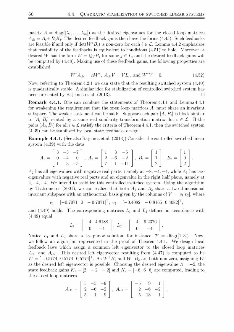
60 4.4. Quadratic stabilization of switched linear systems
matrix Λ = diag([λ1, . . . , λm]) as the desired eigenvalues for the closed loop matricesAcli = Ai+BiKi. The desired feedback gains then have the forms (4.45). Such feedbacksare feasible if and only if det(W ∗Bi) is non-zero for each i ∈ L. Lemma 4.4.2 emphasizesthat feasibility of the feedbacks is equivalent to conditions (4.51) to hold. Moreover, adesired W has the form W = QVBj for some j ∈ L, and the desired feedback gains willbe computed by (4.48). Making use of these feedback gains, the following properties areestablished
W ∗Acli = ΛW ∗, AcliV = V Li, and W ∗V = 0. (4.52)
Now, referring to Theorem 4.2.1 we can state that the resulting switched system (4.40)is quadratically stable. A similar idea for stabilization of controlled switched system hasbeen presented by Bajcinca et al. (2013).
Remark 4.4.1. One can combine the statements of Theorem 4.4.1 and Lemma 4.4.1for weakening the requirement that the open loop matrices Ai must share an invariantsubspace. The weaker statement can be said: “Suppose each pair [Ai Bi] is block similarto [Ai Bi] related by a same real similarity transformation matrix, for i ∈ L. If thepairs (Ai, Bi) for all i ∈ L satisfy the criteria of Theorem 4.4.1, then the switched system(4.39) can be stabilized by local state feedbacks design”.
Example 4.4.1. (See also Bajcinca et al. (2013)) Consider the controlled switched linearsystem (4.39) with the data
A1 =
3 −3 −70 −4 01 3 −5
, A2 =
1 3 −52 −6 −27 1 −11
, B1 =
112
, B2 =
102
.A2 has all eigenvalues with negative real parts, namely at −8,−4,−4, while A1 has twoeigenvalues with negative real parts and an eigenvalue in the right half plane, namely at2,−4,−4. We intend to stabilize this controlled switched system. Using the algorithmby Tsatsomeros (2001), we can realize that both A1 and A2 share a two dimensionalinvariant subspace with an orthonormal basis given by the columns of V = [v1 v2], where
v1 = [−0.7071 0 − 0.7071]>, v2 = [−0.4082 − 0.8165 0.4082]>,
and (4.49) holds. The corresponding matrices L1 and L2 defined in accordance with(4.49) equal
L1 =
[ −4 4.6188
0 −4
], L2 =
[ −4 9.2376
0 −4
].
Notice L1 and L2 share a Lyapunov solution, for instance, P = diag([1, 3]). Now,we follow an algorithm represented in the proof of Theorem 4.4.1. We design localfeedback laws which assign a common left eigenvector to the closed loop matricesAcl1 and Acl2. This desired left eigenvector resulting from (4.47) is computed to beW = [−0.5774 0.5774 0.5774]>. As W>B1 and W>B2 are both non-zero, assigning Was the desired left eigenvector is possible. Choosing the desired eigenvalue Λ = −2, thestate feedback gains K1 = [2 − 2 − 2] and K2 = [−6 6 6] are computed, leading tothe closed loop matrices
Acl1 =
5 −5 −92 −6 −25 −1 −9
, Acl2 =
−5 9 12 −6 −2−5 13 1
.

Chapter 4. Switched linear systems with arbitrary switching signals 61
4.4.2.1 Stabilization for the case of (n − 1) dimensional common invariantsubspace
Consider the special case of the controlled switched linear system (4.39) where the di-mension of the largest common invariant subspace introduced in Theorem 4.4.1 is (n−1)and the system has a single control input. Then, the Ai’s for all i ∈ L share a real lefteigenvector w characterized by
w>V = 0. (4.53)
Note that the open loop matrices are not necessarily Hurwitz, because some eigenvaluesof Ai corresponding to the eigenvector w, denoted by µi1 for i ∈ L, might lie in theright half plane. Therefore, for stabilization of this controlled switched system we preferto shift the eigenvalues µi1 to a point on the negative real axis, while maintaining theother eigenvalues of the matrices Ai unchanged. For this purpose, we use the single shifteigenvalue method elaborated in Chapter 2.2.1.3. Let us denote the desired eigenvaluecorresponding to the left eigenvector w by λ1, and define the vectors bi := Bi with i ∈ Lfor keeping the notation consistent with the one previously introduced. Further, assumew>bi 6= 0 for all i ∈ L. The convenient controller gains then turn out to have the forms
Ki = −(µi1 − λ1)w>
w>bi∀i ∈ L. (4.54)
Now with this control design, Theorem 4.4.1 ensures that the controlled switched system(4.39) is quadratically stable.
Example 4.4.2. Consider again the controlled switched linear system defined in Exam-ple 4.4.1. As explained in that example, both A1 and A2 share a 2 dimensional invariantsubspace. Consequently, they share also a left eigenvector w orthogonal to v1 and v2.This eigenvector is computed as follows:
w = [−0.5774 0.5774 0.5774]>.
Now, we design local state feedback gains each of which only shifts a single eigenvaluecorresponding to the common left eigenvector w of the open loop matrices A1 and A2.As w>B1 and w>B2 are both non-zero, the single shift eigenvalue procedure is possible.Choosing the desired eigenvalue to be λ1 = −2, the same controller gains as the onesderived in Example 4.4.1 result.
4.4.2.2 Stabilization based on (n− 1) common real left eigenvectors
In this part, we plan to incorporate the algorithm developed in Chapters 4.2.1.2 and2.2.2.1 into our stabilization approach for stabilization of controlled switched linear sys-tems with (n−1) control inputs. Our algorithm suggests to assign (n−1) real common lefteigenvectors given by the columns of W = [w1 . . . wn−1] ∈ Rn×(n−1) corresponding to thedesired real stable eigenvalues given by the diagonal elements of Λ = diag([λ1, . . . , λn−1])to the closed loop matrices Acli for all i ∈ L. For the selection of such W , stability ofthe closed loop matrices must be taken into account. For this purpose, we define newvariables W1, . . . ,W`, where Wi = [wi1 . . . wi(n−1)] for i ∈ L are a set of desired left eigen-vectors for Acli, respectively. A common W is obtained whenever W := W1 = · · · = W`.

62 4.4. Quadratic stabilization of switched linear systems
We now employ feedback gains in the form of (4.45). For stability of each closed loopsubsystem, we need that the last eigenvalue of each Acli for i ∈ L, denoted by λin,should also be real negative. It has been shown in Chapter 2.2.2.1 that this condition isequivalent to
λin = −tr(W>i (ai1/(n− 1) I + Ai)Bi(W
>i Bi)
−1)< 0 ∀i ∈ L. (4.55)
We can determine a set of matrices Wi, denoted by Ωi, that satisfy the inequalities (4.55)by using the parameterization method introduced in Chapter 2.2.2.1
W>i =W>i + µiθ
>i ∀i ∈ L,
and follow the algorithm proposed therein. Then, the desired set of W , denoted by Ω,that simultaneously stabilizes all Acli for all i ∈ L, is obtained by intersection of all Ωi,that is, Ω = ∩`i=1Ωi (see Kouhi and Bajcinca (2011c)). The next example illustrateshow this technique can be numerically executed.
Example 4.4.3. Suppose we intend to quadratically stabilize the controlled switchedlinear system (4.39), with the data
A1 =
3 −3 −70 −4 01 3 −5
, A2 =
1 3 −52 −6 −27 1 −11
, B1 =
1 11 02 2
, B2 =
1 21 01 1
.Let the columns of W1 = [w11 w12] and W2 = [w21 w22] be desired left eigenvectors for theclosed loop matrices Acl1 and Acl2, respectively. Note that two common left eigenvectorsgiven by the columns of W = [w1 w2] are obtained when W = W1 = W2. Now, we wantto compute a matrix W such that the closed loop matrices Acl1 and Acl2 constructed bythe state feedback gains in the form of (4.45) are Hurwitz. To this end, we first use theparameterization
W>i =W>i + µiθ
>i i ∈ 1, 2,
where µi and θi are defined in Chapter 2.2.2.1. The parameters θi are computed directlyfrom the equations θ>i Bi = 0 for i ∈ 1, 2
θ1 = [−0.8944 0 0.4472]>, θ2 = [−0.4082 − 0.4082 0.8165]>.
Note that this problem includes several unknown parameters, namely W1, W2, µ1, andµ2. Therefore, for convenience we fix W1 and µ2 to be
W>1 =
[1 1 21 0 2
], µ2 =
[11
],
and compute W2 and µ1 afterwards. From the identity W>1 = W>
2 , we conclude
W>1 + µ1θ>1 =W>2 + µ2θ
>2
⇒W>2 =W>1 + µ1θ>1 − µ2θ
>2 .

Chapter 4. Switched linear systems with arbitrary switching signals 63
This allows us to represent W>2 solely by the unknown parameter µ1 = [µ11 µ12]> as
W>2 =
[1.4082− 0.8944µ11 1.4082 1.1835 + 0.4472µ11
1.4082− 0.8944µ12 0.4082 1.1835 + 0.4472µ12
].
Now, recall from the algorithm presented in Chapter 2.2.2.1 that for stability of the closedloop matrices the following conditions must hold
−Y >1 µ1 − tr(W1X1) < 0, −Y >2 µ2 − tr(W2X2) < 0,
where variables Xi and Yi are defined as follows:
Xi =(ai1/(n− 1) I + Ai
)Bi(W>i Bi)
−1,
Y >i = θ>i
(ai1/(n− 1) I + Ai
)Bi(W>i Bi)
−1,
for each i ∈ 1, 2. X1 and Y1 are known parameters as W1 is given
X>1 =
[−3 −1 31.4 1 −3.6
], Y >1 =
[4.0249 −2.8622
].
X2 and Y2 are parameterized by µ1. Now, we find an appropriate µ1 via solving thefollowing optimization problem:
minimize ‖µ1‖2
subject to
−Y >1 µ1 − tr(W1X1) + γ ≤ 0,
−Y >2 µ2 − tr(W2X2) + γ ≤ 0,
where the positive number γ enters into the problem for ruling out computation of thezero solution for µ1. In this example we assume γ = 0.2. Using the MATLAB command“fmincon” we are able to find a solution for µ1, namely µ1 = [0.6600 − 0.4694]>. Thisidentifies
W> =
[0.4096 1 2.29521.4198 0 1.7901
].
Now, we take the eigenvalues corresponding to the columns of W to be the diagonalentries of Λ = diag([−2,−3]). Thus, the state feedback gains K1 and K2 are computedto be:
K1 =
[5.9656 −2.5458 −3.7658
−8.0274 2.3236 6.4696
], K2 =
[−4.5586 2.9411 6.6617
−0.7727 −3.3458 0.0079
],
and the closed loop matrices are given by
Acl1 =
0.9382 −3.2222 −4.29625.9656 −6.5458 −3.7658−3.1236 2.5557 0.4075
, Acl2 =
−5.1040 −0.7506 1.6774−2.5586 −3.0589 4.66171.6687 0.5953 −4.3305
.
64 4.4. Quadratic stabilization of switched linear systems
The sets of eigenvalues of Acl1 and Acl2 are −0.2,−2,−3 and −7.4933,−2,−3,respectively. This indicates that both matrices are Hurwitz and they share two lefteigenvectors given by the columns of the computed W .
Example 4.4.4. (Kouhi and Bajcinca, 2011c) For the case of n = 2 in the controlledswitched linear system (4.39), we can obtain a simple expressions for stability of theclosed loop matrices. Let’s denote bi := Bi for each i ∈ L, and wi := Wi, where wi is thedesired left eigenvector for the closed loop matrix Acli for each i ∈ L. We can choose λi1any real negative number. Furthermore, recalling (2.8), we must have
λ2i = −w>i (ai1I + Ai)bi
w>i bi< 0 ∀i ∈ L. (4.56)
The criteria (4.56) are met if the inner-products w>i bi and w>i (ai1I+Ai)bi have the samesign. Define Ωi to be the set of all vectors wi that satisfy this condition. Then, theset of a stabilizing common left eigenvector w = w1 = · · · = w`, denoted by Ω, can becomputed by Ω = ∩`i=1Ωi. The region Ωi can be represented geometrically similar towhat were illustrated in Figure 2.2.1.
4.4.3 Stabilization and perturbed invariant subspaces
In this part, we are interested in enlarging the class of controlled switched linearsystems that can be stabilized by left eigenstructure assignment approach. The coreof this section is to show that if all open loop matrices Ai’s with i ∈ L in (4.39) havep := n − m dimensional invariant subspaces which are sufficiently close to each other,we may still be capable of stabilizing the controlled switched system. This argument issubstantiated by accomplishing the proof of the next theorem. Before proceeding, werefer the reader to Appendix A.2.13.1 and Truhar (1996) for the definition of “distancebetween two invariant subspaces”.
Theorem 4.4.2. Define p = n−m. Suppose all Ai’s in the controlled switched system(4.39) possess p-dimensional invariant subspaces Xi,p, such that the distance between Xi,pand Xj,p is sufficiently small for each i, j ∈ L and i 6= j, that is, there exists a smallnumber δ ≥ 0 satisfying
dist (Xi,p,Xj,p) ≤ δ. (4.57)
Moreover, assume that an index j ∈ L and an orthonormal basis with conjugate pairs ofcomplex vectors, given by the columns of a matrix Vj ∈ Cn×p, for the invariant set Xj,pexist such that
rank(B>j QVjBi
)= m ∀i ∈ L, (4.58)
where QVj = I − VjV ∗j . For each i ∈ L and i 6= j, let the columns of Vi ∈ Cn×p be anormal basis (not necessarily orthogonal) for Xi,p, satisfying
AiVi = ViLi, ‖Vi − Vj‖2 ≤√
2p dist(Xi,p,Xj,p), (4.59)

Chapter 4. Switched linear systems with arbitrary switching signals 65
where ‖.‖2 indicates the induced 2-norm (see Appendix A.2.11). Then, if there existscalars γ1, γ2 > 0 and a Hermitian positive definite matrix P ∈ Cp×p, i.e., P = P∗ > 0,such that the following Riccati inequalities hold
L∗iP + PLi + γ21P2 + γ2
2Ip < 0 ∀i ∈ L, (4.60)
and the number γ1γ2 is sufficiently large, the controlled switched system (4.39) can bestabilized by local state feedback controller design.
Proof: The proof consists of two parts. In part A, we show that a Vi ∈ Cn×p exists, suchthat its columns form a basis for the invariant subspace Xi,p and simultaneously satisfy(4.59). In Part B we demonstrate that if (4.60) holds and γ1γ2 is sufficiently large, thenthe controlled switched linear system (4.39) can be quadratically stabilized.
Part A: Fix a j ∈ L and an orthonormal matrix V := Vj ∈ Cn×p such that (4.58) holds.Let’s define an orthonormal matrix Φi ∈ Cn×m such that its columns are perpendicularto the space Xi,p. It is obvious that
Xi,p = x ∈ Cn : Φi∗x = 0 ∀i ∈ L. (4.61)
The projection of a vector vk, the k-th column of V for k ∈ 1, . . . , p, onto the set Xi,pequals
ProjXi,p(vk) = (In − ΦiΦi∗)vk ∀k ∈ 1, . . . , p;
see Appendix A.8.1. Now, we define the following normal vectors
vik =1
‖(In − ΦiΦi∗)vk‖
(In − ΦiΦi∗)vk ∀k ∈ 1, . . . , p, (4.62)
and the collection of them as Vi = [vi1 . . . vip] for i ∈ L. We claim that Vi is defined, itscolumn vectors are linearly independent and form a basis for the set Xi,p for each i ∈ L.To see this, first notice that the following identity is valid
(In − ΦiΦi∗)[V 0] = (In − ΦiΦi
∗)[V Φi].
On the other hand, we should have rank([V Φi]) = n; otherwise, there must exist avector φi ∈ Cn such that φ∗i [V Φi] = 0, implying that both φ∗iV = 0 and φ∗iΦi = 0 musthold. Next, referring to (4.61) the expression φ∗iΦi = 0 implies that φi ∈ Xi,p, and theexpression φ∗iV = 0 implies that φi is perpendicular to all vectors in the space Xj,p. Butthis is impossible since the canonical angle between Xi,p and Xj,p is assumed to be small.Now, we have
rank (Vi) = rank ((In − ΦiΦi∗)V ) = rank ((In − ΦiΦi
∗)[V 0])
= rank ((In − ΦiΦi∗)[V Φi]) = rank(In − ΦiΦi
∗) = p. (4.63)
Next, note that by the definition of vik in (4.62), we can deduce
mink∈1,...,p
v∗kvik = minvk∈v1,...,vp
maxνi∈Xi,p
v∗kνi ≥ minv∈Xj,p
maxνi∈Xi,p
v∗νi = cos(θij), (4.64)

66 4.4. Quadratic stabilization of switched linear systems
where θij is the maximum canonical angle between two spaces Xi,p and Xj,p; see Ap-pendix A.2.13.1. Let’s define ∆Vi := V − Vi for each i ∈ L with i 6= j. Then,
‖∆Vi‖22 = ‖V − Vi‖2
2 = σmax(∆Vi)2 ≤ tr (∆V ∗i ∆Vi) ≤ p max
k∈1,...,p(‖vk − vik‖2);
see Appendix A.2.11. Then, we have
‖∆Vi‖22 ≤ p max
k∈1,...,p(‖vk − vik‖2) = p max
k∈1,...,p(2− 2v∗kvik) =
= 2p(
1− mink∈1,...,p
(v∗kvik)). (4.65)
Now, referring to (4.64) we can write
‖∆Vi‖2 ≤ 2p (1− minv∈Xj,p
maxνi∈Xi,p
(v∗νi)) = 2p(1− cos(θij)), (4.66)
where θij is the greatest canonical angle between Xi,p and Xj,p. On the other hand, using2sin2(θij/2) = 1− cos(θij), we deduce that
‖∆Vi‖2 ≤ 4p sin2(θij/2).
As θij < π/2, the inequality sin(θij/2) ≤ cos(θij/2) is valid. Hence,
‖∆Vi‖2 ≤ 4p sin(θij/2) cos(θij/2) = 2p sin(θij) = 2p dist (Xi,p,Xj,p) . (4.67)
Part B: Now, choosing appropriate matrices Vi for all i ∈ L with regard to the discussionin Part A, we introduce our stabilization method. We choose the columns of W = QVBj
as the set of desired left eigenvectors corresponding to m desired eigenvalues comingwith complex conjugate pairs in the open left half plane given by the diagonal entriesof Λ = diag([λ1, . . . , λm]) for the closed-loop matrix Acli = Ai + BiKi. Referring toLemma 4.4.2, we can argue that W can be assigned to Acli if (4.58) holds. Then, thedesired controller gain Ki has the form (4.48). Next, define the reduced QR-factorizationW = Q1R1, where R1 is an m ×m upper triangular non-singular matrix and Q1 is ann×m matrix which has orthonormal columns. Choosing the orthonormal transformationmatrix T = [Q1 V ], we can define a set of Acli’s which are similar to Acli’s as follows:
Acli = T ∗AcliT =
[R−∗1 ΛR∗1 0V ∗AcliQ1 V ∗AcliV
]∀i ∈ L.
We take a common Lyapunov solution for Acli, i ∈ L, in the form of
P = 12
[R1R
∗1 0
0 εP
],
where P = P∗ ∈ Cp×p is defined in accordance with (4.60). The Lyapunov equation forthe transformed matrices Acli equals
A∗cliP + P Acli =
[R1Re(Λ)R∗1
ε2Q∗1A
>cliV P
ε2PV ∗AcliQ1
ε2(PV ∗AcliV + V ∗A>cliV P)
]∀i ∈ L. (4.68)

Chapter 4. Switched linear systems with arbitrary switching signals 67
As R1Re(Λ)R∗1 < 0, (4.68) is negative definite if and only if Si < 0, where Si stands forits Schur complement with respect to the upper left block as
Si = ε2(PV ∗AcliV + V ∗A>cliV P)− ε2
4(PV ∗AcliQ1) (R1Re(Λ)R∗1)−1 (Q∗1A
>cliV P). (4.69)
Following the proof of Theorem 4.4.1, for a sufficiently small ε > 0, the inequality Si < 0is satisfied if and only if
PV ∗AcliV + V ∗A>cliV P < 0 ∀i ∈ L. (4.70)
We prove the last inequality holds if ‖∆Vi‖2 is sufficiently small. First, note that usingthe feedback gain of the form (4.48), the identity
AcliV =[Ai −Bi(B
>j QVBi)
−1(B>j QVAi − ΛB>j QV )]V
=[I −Bi(B
>j QVBi)
−1B>j QV]AiV = AiV + EiV (4.71)
holds, where we have defined
Ei := −Bi(B>j QVBi)
−1B>j QVAi.
Now, recall that ∆Vi is defined as ∆Vi := V − Vi, where Vi is defined by (4.62). Thus,the property (4.59) also holds. Consequently, the matrices Li for all i ∈ L in (4.59) aredefined and available. Now, suppose a suitable P can be determined such that (4.60)holds. Then, part of the Lyapunov equation for this mode can be written in the form of
PV ∗AcliV = PV ∗(Ai + Ei)V
= P(V − Vi(V ∗i Vi)−1 + Vi(V∗i Vi)
−1)∗Ai(Vi + ∆Vi) + PV ∗EiV= P(V ∗i Vi)
−1V ∗i AiVi + P(V − Vi(V ∗i Vi)−1)∗AiV + P(V ∗i Vi)−1V ∗i Ai∆Vi + PV ∗EiV
= P(V ∗i Vi)−1V ∗i ViLi + P(V − Vi(V ∗i Vi)−1)∗AiV + P(V ∗i Vi)
−1V ∗i Ai∆Vi + PV ∗EiV= PLi + P(V − Vi(V ∗i Vi)−1)∗AiV + P(V ∗i Vi)
−1V ∗i Ai∆Vi + PV ∗EiV= PLi + PFi,
where we have defined Fi as
Fi := (V − Vi(V ∗i Vi)−1)∗AiV + (V ∗i Vi)−1V ∗i Ai∆Vi + V ∗EiV. (4.72)
Referring to (4.60), we can write
PV ∗AcliV + V ∗A>cliV P = PLi + L∗iP + PFi + F ∗i P <
− γ21P2 + PFi + F ∗i P − γ2
2Ip =
−(γ1P −
1
γ1
Fi
)∗(γ1P −
1
γ1
Fi
)+[
1γ21F ∗i Fi − γ2
2Ip
].
The first summand of the above expression is clearly negative semi-definite. We willshow also when ∆Vi is small, the second summand is negative semi-definite. To this end,for a small value of ‖∆Vi‖, we should show
1γ21F ∗i Fi − γ2
2Ip ≤ 0⇒ σmax(Fi) ≤ γ1γ2.

68 4.4. Quadratic stabilization of switched linear systems
On the other hand, referring to the definition of Fi in (4.72), σmax(Fi) is bounded by
σmax(Fi) ≤ σmax
((V − Vi(V ∗i Vi)−1)∗AiV + V ∗EiV
)+ σmax
((V ∗i Vi)
−1V ∗i Ai∆Vi)
≤ σmax
((V − Vi(V ∗i Vi)−1)∗AiV + V ∗EiV
)+ σmax
((V ∗i Vi)
−1V ∗i Ai)‖∆Vi‖2.
Hence, if the norm of the perturbation ∆Vi is bounded by
‖∆Vi‖2 = σmax(∆Vi) ≤γ1γ2 − σmax (V ∗(Ai + Ei)V − (V ∗i Vi)
−1V ∗i AiV )
σmax ((V ∗i Vi)−1V ∗i Ai)
, (4.73)
then the switched system (4.39) is stable. Recalling (4.71), if γ1γ2 is sufficiently large sothat the inequalities γ1γ2 ≥ σmax (V ∗AcliV − (V ∗i Vi)
−1V ∗i AiV ) for all i ∈ L hold, and thedistances between the invariant subspaces Xi,p and Xj,p are less than or equal to someδ ≥ 0, for instance,
dist (Xi,p,Xj,p) ≤ δ, δ :=1
2pmini∈Li6=j
(γ1γ2 − σmax (V ∗AcliV − (V ∗i Vi)
−1V ∗i AiV )
σmax ((V ∗i Vi)−1V ∗i Ai)
)2
, (4.74)
then (4.73) and (4.67) are satisfied. Therefore, quadratic stability of the closed loopswitched linear system (4.39) is deduced.
Example 4.4.5. Consider again the controlled switched linear system (4.39), with thesame matrices A1, B1, and B2 presented in Example 4.4.1. However, we assume that thematrix A2 has been slightly perturbed in the form of
A2 =
1 3 −52 −6 −27 1 −11
+ 10−4 ×
1 2 −12 −1 −17 1 −2
.After finding the two dimensional invariant subspaces of matrices A1 and A2, we realizethat the two dimensional invariant subspaces X1,2 and X2,2 defined by
Xi,2 = x ∈ C3 : Φi∗x = 0 i ∈ 1, 2,
where
Φ1 = [−0.5774 0.5774 0.5774]>, Φ2 = [−0.5658+0.1148i 0.5660−0.1149i 0.5657−0.1148i]>,
corresponding to A1 and A2, respectively, have a fairly small distance dist(X1,2−X2,2) =3.2314× 10⁻⁴. The orthonormal vectors given by the columns of V = [v1 v2] computedin Example 4.4.1 form a basis for X1,2. Likewise, the vectors given by the columns ofV2 = [v21 v22] with v2k = (I3 −Φ2Φ2
∗)vk/‖(I3 −Φ2Φ2∗)vk‖ for k ∈ 1, 2 form a normal
basis for X2,2. These vectors are numerically given by
v21 = [−0.7071 0 − 0.7071]>,
v22 = [−0.4084 − 0.8164 0.4084]>.
Furthermore, one can realize that
‖V − V2‖ = 2.8794× 10⁻⁴ <√
4 dist(X1,2 −X2,2) = 0.0360.
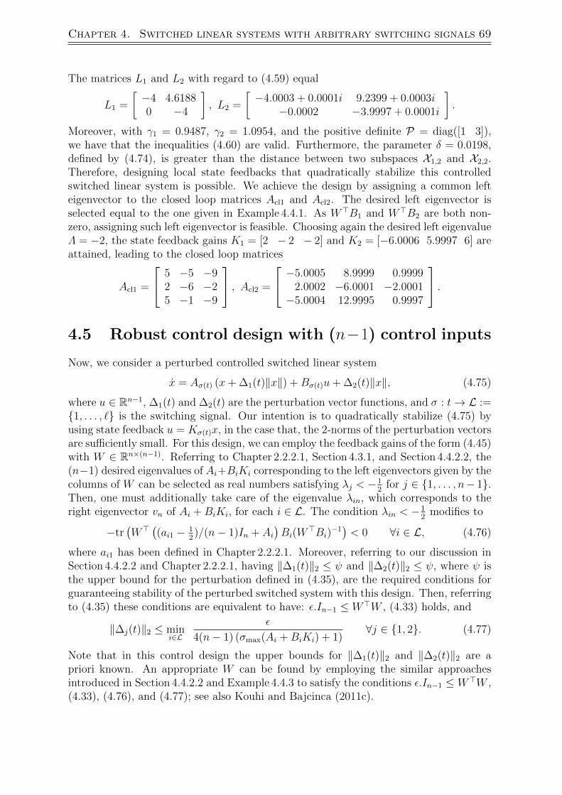
Chapter 4. Switched linear systems with arbitrary switching signals 69
The matrices L1 and L2 with regard to (4.59) equal
L1 =
[−4 4.61880 −4
], L2 =
[−4.0003 + 0.0001i 9.2399 + 0.0003i
−0.0002 −3.9997 + 0.0001i
].
Moreover, with γ1 = 0.9487, γ2 = 1.0954, and the positive definite P = diag([1 3]),we have that the inequalities (4.60) are valid. Furthermore, the parameter δ = 0.0198,defined by (4.74), is greater than the distance between two subspaces X1,2 and X2,2.Therefore, designing local state feedbacks that quadratically stabilize this controlledswitched linear system is possible. We achieve the design by assigning a common lefteigenvector to the closed loop matrices Acl1 and Acl2. The desired left eigenvector isselected equal to the one given in Example 4.4.1. As W>B1 and W>B2 are both non-zero, assigning such left eigenvector is feasible. Choosing again the desired left eigenvalueΛ = −2, the state feedback gains K1 = [2 − 2 − 2] and K2 = [−6.0006 5.9997 6] areattained, leading to the closed loop matrices
Acl1 =
5 −5 −92 −6 −25 −1 −9
, Acl2 =
−5.0005 8.9999 0.99992.0002 −6.0001 −2.0001−5.0004 12.9995 0.9997
.4.5 Robust control design with (n−1) control inputs
Now, we consider a perturbed controlled switched linear system
x = Aσ(t) (x+ ∆1(t)‖x‖) +Bσ(t)u+ ∆2(t)‖x‖, (4.75)
where u ∈ Rn−1, ∆1(t) and ∆2(t) are the perturbation vector functions, and σ : t→ L :=1, . . . , ` is the switching signal. Our intention is to quadratically stabilize (4.75) byusing state feedback u = Kσ(t)x, in the case that, the 2-norms of the perturbation vectorsare sufficiently small. For this design, we can employ the feedback gains of the form (4.45)with W ∈ Rn×(n−1). Referring to Chapter 2.2.2.1, Section 4.3.1, and Section 4.4.2.2, the(n−1) desired eigenvalues of Ai+BiKi corresponding to the left eigenvectors given by thecolumns of W can be selected as real numbers satisfying λj < −1
2for j ∈ 1, . . . , n− 1.
Then, one must additionally take care of the eigenvalue λin, which corresponds to theright eigenvector vn of Ai +BiKi, for each i ∈ L. The condition λin < −1
2modifies to
−tr(W> ((ai1 − 1
2)/(n− 1)In + Ai
)Bi(W
>Bi)−1)< 0 ∀i ∈ L, (4.76)
where ai1 has been defined in Chapter 2.2.2.1. Moreover, referring to our discussion inSection 4.4.2.2 and Chapter 2.2.2.1, having ‖∆1(t)‖2 ≤ ψ and ‖∆2(t)‖2 ≤ ψ, where ψ isthe upper bound for the perturbation defined in (4.35), are the required conditions forguaranteeing stability of the perturbed switched system with this design. Then, referringto (4.35) these conditions are equivalent to have: ε.In−1 ≤ W>W , (4.33) holds, and
‖∆j(t)‖2 ≤ mini∈L
ε
4(n− 1) (σmax(Ai +BiKi) + 1)∀j ∈ 1, 2. (4.77)
Note that in this control design the upper bounds for ‖∆1(t)‖2 and ‖∆2(t)‖2 are apriori known. An appropriate W can be found by employing the similar approachesintroduced in Section 4.4.2.2 and Example 4.4.3 to satisfy the conditions ε.In−1 ≤ W>W ,(4.33), (4.76), and (4.77); see also Kouhi and Bajcinca (2011c).
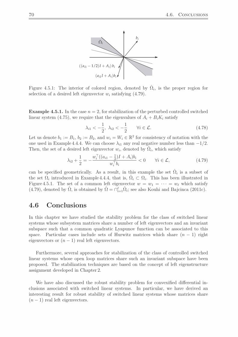
70 4.6. Conclusions
bi
(ai1 I + Ai)bi
((ai1 − 1/2)I + Ai) bi
Ωi
Figure 4.5.1: The interior of colored region, denoted by Ωi, is the proper region forselection of a desired left eigenvector wi satisfying (4.79).
Example 4.5.1. In the case n = 2, for stabilization of the perturbed controlled switchedlinear system (4.75), we require that the eigenvalues of Ai + BiKi satisfy
λi1 < −1
2, λi2 < −1
2∀i ∈ L. (4.78)
Let us denote b1 := B1, b2 := B2, and wi = Wi ∈ R2 for consistency of notation with the
one used in Example 4.4.4. We can choose λi1 any real negative number less than −1/2.Then, the set of a desired left eigenvector wi, denoted by Ωi, which satisfy
λi2 +1
2= −w
i ((ai1 − 1
2)I + Ai)bi
wi bi
< 0 ∀i ∈ L, (4.79)
can be specified geometrically. As a result, in this example the set Ωi is a subset ofthe set Ωi introduced in Example 4.4.4, that is, Ωi ⊂ Ωi. This has been illustrated inFigure 4.5.1. The set of a common left eigenvector w = w1 = · · · = w which satisfy(4.79), denoted by Ω, is obtained by Ω = ∩
i=1Ωi; see also Kouhi and Bajcinca (2011c).
4.6 Conclusions
In this chapter we have studied the stability problem for the class of switched linearsystems whose subsystem matrices share a number of left eigenvectors and an invariantsubspace such that a common quadratic Lyapunov function can be associated to thisspace. Particular cases include sets of Hurwitz matrices which share (n − 1) righteigenvectors or (n− 1) real left eigenvectors.
Furthermore, several approaches for stabilization of the class of controlled switchedlinear systems whose open loop matrices share such an invariant subspace have beenproposed. The stabilization techniques are based on the concept of left eigenstructureassignment developed in Chapter 2.
We have also discussed the robust stability problem for convexified differential in-clusions associated with switched linear systems. In particular, we have derived aninteresting result for robust stability of switched linear systems whose matrices share(n− 1) real left eigenvectors.

Chapter 5. Rank-m difference switched systems 71
Chapter 5
Rank-m difference switched systems
5.1 Introduction
In this chapter, we introduce a tractable condition on pairs of Hurwitz matrices A1 andA2, which guarantees existence of a common Lyapunov solution for them. While it turnsout that A1A2 having no real negative eigenvalue (spectral condition) is a necessarycondition for the existence of a common Lyapunov solution for A1 and A2 (Shortenand Narendra, 2003), this condition is not sufficient. An example that this necessarycondition fails to be sufficient is as follows:
A1 =
−1.8 0.5 0.1 0.4
0.1 −1.8 0.1 0.90.1 0.7 0.6 −2.10.1 0.8 0.9 −1.8
, A2 =
−1.8 0.1 0.9 0.3
0.2 −0.4 −1.7 0.3−0.4 0.7 1.1 −2
0.4 0.6 0.8 −2.8
. (5.1)
A1 and A2 are both Hurwitz, and the eigenvalues of the product A1A2 are4.696, 0.6303 ± 1.5505i, 0.2333. Thus, no real negative eigenvalue for A1A2 exists.However, by using a suitable software, it can be checked that no common solutionP = P> > 0 for the Lyapunov inequalities A>i P + PAi < 0, i ∈ 1, 2, exists.
Therefore, we are interested to characterize a class of matrices that given abovespectral condition is also sufficient for the existence of such a solution. An initial resultin this direction has been given by Shorten and Narendra (2003), stating that anytwo matrices which are Hurwitz, differ by a rank-1 matrix, and satisfy the spectralcondition possess a common Lyapunov solution. In the proof of this result, a transferfunction is associated with A1 and A2. This transfer function is demonstrated to beStrictly Positive Real (SPR). Existence of a common Lyapunov solution for the pairof matrices then results from the Kalman-Yakubovic-Popov (KYP) lemma (see Zhouet al. (1996)) which is tight for the class of SPR systems. Despite much effort, it hasnot been possible to extend this result to more general pairs of matrices until recently(Kouhi et al., 2013a).
In this chapter, we introduce a new pair of matrices for which the above spectralcondition is both sufficient and necessary for having a common Lyapunov solution andthus guaranteeing stability of the switched system x = Aσ(t)x, σ(t) ∈ 1, 2. These are
72 5.2. Symmetric transfer function matrices
pairs of stable matrices which are related by a symmetric transfer function matrix. Fordeveloping the results, we follow a similar approach to the existing one for the class ofrank-1 difference matrices.
5.2 Symmetric transfer function matrices
Symmetric transfer function matrices can be found in many applications. For example,symmetric transfer functions are ubiquitous in the study of electrical systems (Helmkeet al., 2006; Semlyen and Gustavsen, 2009), in systems with collocated sensors and actu-ators (Yang and Qiu, 2002), and in chemical process plants (Shinskey, 1984; Hovd andSkogestad, 1994; Kouhi et al., 2014). Due to this wide range of applications, numerousresults concerning control design for this class of systems exist in the literature; see,e.g., Shinskey (1984); Hovd and Skogestad (1994); Xie et al. (2004); Fuhrmann (1983).In this part, however, we study this class of systems solely from a mathematical pointof view. In fact, the mathematical properties of symmetric transfer function matri-ces play an integral role for the stability theory of switched linear systems in this chapter.
We begin by exploring conditions on the matrix components of a state spacerealization (A,B,C,D) characterizing a symmetric transfer function matrixG(s) = C(sI − A)−1B + D. Lemma 5.2.1 represents a necessary and sufficientcondition for symmetric transfer function matrices with respect to Markov parameters,while Lemma 5.2.2 establishes a link between the symmetry condition and similar statespace realizations. In Lemma 5.2.4 we introduce one of the important properties thatsymmetric transfer function matrices exhibit.
Throughout this chapter we always assume that A ∈ Rn×n, B ∈ Rn×m has fullcolumn rank, C ∈ Rm×n has full row rank, and D ∈ Rm×m for some m ≤ n.
Lemma 5.2.1. (See, e.g., Kouhi et al. (2013a)) The transfer function matrix G(s) =C(sI − A)−1B +D is symmetric, that is, G(s) = G>(s) if and only if
D = D>,
CAiB = (CAiB)> ∀i ∈ 0, 1, . . . , n− 1. (5.2)
Proof: Let’s define the characteristic polynomial of A as
det(λI − A) = λn + a1λn−1 + a2λ
n−2 + · · ·+ an.
Then, referring to (Kailath (1980), pp.67), the following identity holds
C(sI − A)−1B =1
det(sI − A)[sn−1(CB) + sn−2(CAB +a1CB)+
· · ·+ (CAn−1B +· · ·+ an−1CB)].
Hence, it is immediately evident that the condition (5.2) and the assumption D = D>
are necessary and sufficient for the transfer function matrix G(s) = C(sI − A)−1B +D

Chapter 5. Rank-m difference switched systems 73
to be symmetric.
We say that the dynamic systems x = Ax and x = (A − BD−1C)x, where matricesA, B, C, and D satisfy the property of Lemma 5.2.1, are generators of the symmetrictransfer function matrix G(s) = C(sI − A)−1B +D; see Kouhi et al. (2013a).
Lemma 5.2.2. See Kailath (1980). Let (A,B,C,D) be a minimal realization of thetransfer function matrix G(s) = C(sI − A)−1B + D. Then G(s) is symmetric, if andonly if there exists a unique invertible matrix S> = S (not necessarily positive definite),such that
A>S = SA, C = B>S, and D = D>. (5.3)
Proof of necessity: This proof can be found in Kailath (1980); Willems (1972). AsG(s) and
G>(s) = B>(sI − A>)−1C> +D>
are equal, the minimal state space realizations (A,B,C,D) and (A>, C>, B>, D>) aresimilar. This implies that a non-singular unique matrix S exists such that
A> = SAS−1, C> = SB, B> = CS−1, and D> = D.
Therefore, A>S = SA and C = B>S. In addition, we have A>S> = S>A and C =B>S>. This means that S is not unique, unless we have S = S>.
Proof of sufficiency: Suppose there exists a unique invertible symmetric matrix S,such that (5.3) holds. Substituting C = B>S into G(s), and paying attention that in
G(s) = C(sI − A)−1B +D = B>(s S−1 − AS−1)−1B +D (5.4)
S−1, AS−1, and D are symmetric, symmetry of G(s) results. Note that (5.4) in factrepresents the descriptor form of G(s); see Knockaert et al. (2013).
As discussed in the introduction of this chapter, we are interested in developingresults for switched systems associated with symmetric transfer function matrices. Thebasic question now is how to specify the class of matrix pairs A1 and A2, such that asymmetric transfer function can be associated with them? The following lemma providesa tool for specifying this class. Before proceeding, note that ⊗ denotes the Kroneckerproduct of two matrices; see Appendix A.2.4.
Lemma 5.2.3. (See also Kouhi et al. (2014)) Given two matrices A1 ∈ Rn×n andA2 ∈ Rn×n with the controllable pair (A1, A1−A2), a symmetric transfer function matrixG(s) = C(sI − A)−1B + D with the minimal realization (A,B,C,D) can be associatedwith A1 and A2 such that
A1 := A and A2 = A−BD−1C, (5.5)

74 5.2. Symmetric transfer function matrices
if and only if the matrices
E1 := In ⊗ A1 − A1 ⊗ In and
E2 := In ⊗ A2 − A2 ⊗ In (5.6)
share a right eigenvector corresponding to a zero eigenvalue, say
vec(Y ) = [y11 . . . yn1 y12 . . . yn2 . . . y1n . . . ynn]>,
such that
Y =
y11 y12 . . . y1n...
... . . ....
yn1 yn2 . . . ynn
(5.7)
is symmetric and invertible, and (A1 − A2)Y is positive semi-definite.
Proof of necessity: Define A := A1. Suppose there exist matrices B, C, and D suchthat G(s) = C(sI −A)−1B +D is symmetric, (A,B,C,D) is a minimal realization, andA2 = A − BD−1C. Then, referring to Lemma 5.2.2 there exists a matrix S = S>, suchthat
A>S − SA = 0, B>S = C. (5.8)
Replacing C from (5.8) into (5.5), we get
A2 = A−BD−1B>S ⇒ A2S−1 = AS−1 −BD−1B>. (5.9)
Notice (5.8) reveals that AS−1 = S−1A>. This implies that AS−1 − BD−1B> is sym-metric, and therefore from (5.9) we conclude that A2S
−1 is symmetric as well, thatis,
A2S−1 − S−1A>2 = 0. (5.10)
Defining Y = S−1, both A and A2 satisfy the following Sylvester equations
AY − Y A> = 0, A2Y − Y A>2 = 0. (5.11)
For finding a solution of these equations, utilizing the Kronecker product notation andthe vectorization operator vec(Y ) = [y11 . . . yn1 y12 . . . yn2 . . . y1n . . . ynn]>, we canreformulate (5.11) in the form of
(In ⊗ A1 − A1 ⊗ In) vec(Y ) = 0,
(In ⊗ A2 − A2 ⊗ In) vec(Y ) = 0; (5.12)
see Horn and Johnson (1990). It is obvious that (5.12) implies E1 = (In⊗A1−A1⊗ In)and E2 = (In⊗A2−A2⊗In) share a right eigenvector corresponding to a zero eigenvalue,where its associated matrix Y is symmetric and invertible, and (A1 −A2)Y = BD−1B>

Chapter 5. Rank-m difference switched systems 75
is positive semi-definite. Note that as both E1 and E2 are singular, they both have zeroeigenvalues.
Proof of sufficiency: Suppose E1 and E2 share an eigenvector corresponding to azero eigenvalue, say vec(Y ), such that the matrix Y = [yij] ∈ Rn×n defined by (5.7)is symmetric and invertible (Note that the assumption for Y to be symmetric is notrestrictive. In fact, if X is a solution to A1X −XA>1 = 0, then (XA>1 )> = (A1X)> andA1(X + X>) = XA>1 + (A1X)> = XA>1 + X>A>1 = (X + X>)A>1 . It follows that thesymmetric matrix (X +X>) is also a solution to the equation A1X −XA>1 = 0). Then,taking A := A1, Y satisfies (5.11). This implies that the matrix (A−A2)Y is symmetric.Suppose rank ((A− A2)Y ) = m. As (A− A2)Y is symmetric and by the assumption ofthis lemma is positive semi-definite, its eigenvalue decomposition can be written as
(A− A2)Y = T>ΛT, (5.13)
where T> = T−1 ∈ Rn×n and Λ ∈ Rn×n is a diagonal matrix with exactly n −m zeroelements; see Appendix A.2.7. Therefore, there exists a diagonal matrix Λ1 ∈ Rm×n suchthat Λ = Λ>1 Λ1. Consequently, we can write
(A− A2)Y = T>ΛT = (Λ1T )>(Λ1T ).
Defining S = Y −1, and
B = (Λ1T )>, C = B>S, and D = I, (5.14)
we have
A− A2 = (Λ1T )>(Λ1T )Y −1 = BD−1C
⇒ A2 = A−BD−1C, (5.15)
and G(s) = C(sI−A)−1B+D is symmetric. For proving that (A,B,C,D) is a minimalrealization of G(s), first note that
rank Φc(A,B) = rank([B AB . . . An−1B]
)≥ rank
([B AB . . . An−1B](In ⊗B>S)
)= rank
([BB>S ABB>S . . . An−1BB>S]
)= rank
([(A− A2) A(A− A2) . . . An−1(A− A2)]
)= rank Φc(A,A− A2) = n,
where Φc is the controllability matrix; see Appendix A.3. On the other hand, rank of theobservability matrix Φo(C,A) equals
rank Φo(C,A) = rank Φc(A>, C>) = rank Φc(A
>, SB)
= rank([SB A>SB . . . (A>)n−1SB]
)= rank
([SB SAB . . . SAn−1B]
)= rank (S Φc(A,B)) = n;
see Appendix A.4. This implies that (A,B) is controllable and (C,A) is observable, andthus (A,B,C,D) is a minimal realization of G(s).
76 5.2. Symmetric transfer function matrices
Remark 5.2.1. If the eigenvalues of A1 are λ1, . . . , λn, then the eigenvalues of E1
defined in (5.6) are λi − λj for all i, j ∈ 1, . . . , n; see Horn and Johnson (1990).Therefore, E1 has at least n zero eigenvalues. Likewise, such a property holds for E2.However, this does not imply that E1 and E2 share an eigenvector corresponding to azero eigenvalue.
As a result, if two real matrices A1 and A2 are given and one wishes to check whether asymmetric transfer function matrix can be associated with them, the following algorithmcan be utilized:
i) compute a common eigenvector vec(Y ), corresponding to a zero eigenvalue (if oneexists) of the matrices E1 := (In ⊗ A1 − A1 ⊗ In) and E2 = (In ⊗ A2 − A2 ⊗ In).
ii) compute Y by re-arranging vec(Y ). If Y is symmetric and invertible, and (A−A2)Yis positive semi-definite, then associating a symmetric transfer function matrix withA1 and A2 is possible.
iii) define A := A1, and compute the eigenvalue decomposition of (A − A2)Y . Thisdefines matrices T and Λ1 which satisfy (A− A2)Y = T>Λ>1 Λ1T .
iv) compute B, C, and D in accordance with (5.14).
The following example illustrates the steps of the algorithm.
Example 5.2.1. Consider the two matrices
A1 =
[−1 0
5 −1
], A2 =
[1.5 −1.37.5 −5
]. (5.16)
The matrices E1 := (I2 ⊗A1 −A1 ⊗ I2) and E2 := (I2 ⊗A2 −A2 ⊗ I2) are computed asfollows:
E1 =
0 0 0 05 0 0 0−5 0 0 0
0 −5 5 0
, E2 =
0 −1.3 1.3 0
7.5 −6.5 0 1.3−7.5 0 6.5 −1.3
0 −7.5 7.5 0
. (5.17)
A common eigenvector vec(Y ) corresponding to a zero eigenvalue such that Y is sym-metric exists and equals
vec(Y ) = [0 1 1 5]>.
The matrix Y resulting from re-arrangement of vec(Y )
Y =
[0 11 5
],
is invertible and symmetric. Defining A := A1, we have that
(A− A2)Y =
[1.3 44 17.5
]

Chapter 5. Rank-m difference switched systems 77
is positive definite. Next, from the eigenvalue decomposition of (A − A2)Y and using(5.14), we compute
B =
[−0.5892783 −0.97608970.1375708 −4.1810375
], C =
[3.0839625 −0.58927830.6994109 −0.9760897
], D = I.
Therefore, we can associate a symmetric transfer function matrix with A1 and A2 as
G(s) = C(sI − A)−1B +D =1
(s+ 1)2
[s2 + 0.0102s+ 0.838 2.33− 0.546s
2.33− 0.546s s2 + 5.4s+ 9.162
].
Note that such a symmetric transfer function matrix associated with A1 and A2 is notunique. For instance, in this example we can choose
B =
[1 210 5
], C =
[1 0.2−1 0.4
], D =
[2 00 0.667
].
This leads to the symmetric transfer function matrix
G(s) = C(sI − A)−1B +D =1
(s+ 1)2
[2s2 + 7s+ 6 5 + 3s
5 + 3s 0.667s2 + 1.333s+ 4.667
].
Symmetric transfer function matrices and SISO transfer functions share many prop-erties. In particular, we note the following result which is shared by both system classes.
Lemma 5.2.4. (Kouhi et al., 2014) For any symmetric transfer function matrix G(s) =C(sI − A)−1B +D with D = D>, the following equality holds
1
2G(jω) +G>(−jω) = D − C(ω2I + A2)−1AB.
Proof: First, by considering the identity
(jωI − A)−1A = A(jωI − A)−1,
the following relationship holds
12(jωI − A)−1 + (−jωI − A)−1 =
= 12(−jωI − A)−1 (−jωI − A) + (jωI − A) (jωI − A)−1
= −(−jωI − A)−1A(jωI − A)−1
= −(−jωI − A)−1(jωI − A)−1A
= −(ω2I + A2)−1A.
Therefore, as D = D> we can write
1
2G(jω) +G(−jω) =
=1
2D + C(jωI − A)−1B+
1
2D + C(−jωI − A)−1B =
= D +1
2C(jωI − A)−1 + (−jωI − A)−1B = D − C(ω2I + A2)−1AB.

78 5.3. Strictly Positive Real systems (SPR)
5.3 Strictly Positive Real systems (SPR)
Now, we describe the concept of strictly positive real systems, which plays a crucial rolein our stability analysis of switched linear systems. For this reason, in this section westudy some properties of such systems in the context of linear time invariant systems.
Definition 5.3.1. (See, e.g., Corless and Shorten (2010)) An m ×m rational transferfunction matrix G(s) = C(sI − A)−1B + D is said to be strictly positive real (SPR), ifthere exists an α > 0 such that G(s) is analytic in the region of the complex plane whichincludes all s for which Re(s) ≥ −α and
G(jω − α) +G>(−jω − α) ≥ 0 ∀ω ∈ R. (5.18)
The following characterization, inspired principally by Narendra and Taylor (1973),provides a more convenient description of an SPR transfer function matrix.
Lemma 5.3.1. (Corless and Shorten, 2010) Given A Hurwitz, an m×m rational transferfunction matrix G(s) = C(sI − A)−1B +D is strictly positive real if and only if
G(jω) +G>(−jω) > 0 ω ∈ R, (5.19)
and
limω→∞
ω2(m−p)det(G(jω) +G>(−jω)
)> 0, (5.20)
where p = rank(G(∞) +G>(∞)
).
Now, we present some results concerning strictly positive real systems which havesymmetric transfer function matrices.
5.3.1 Symmetric SPR systems with nonsingular D
For symmetric transfer function matrices with invertible D, we have the following simpleresult.
Theorem 5.3.1. (Kouhi et al., 2013a; Semlyen and Gustavsen, 2009) Given a Hurwitzmatrix A, the symmetric transfer function matrix G(s) = C(sI − A)−1B + D withD = D> > 0 is SPR if and only if A(A−BD−1C) has no real negative eigenvalue.
Proof of sufficiency: Suppose A(A − BD−1C) has no real negative eigenvalue, wedemonstrate that G(s) is SPR. By continuity of det (ω2I + A(A−BD−1C)) with respectto ω everywhere, we can write
det(ω2I + A(A−BD−1C)) > 0 (5.21)
⇒ det(ω2I + A2)det(I − (ω2I + A2)−1ABD−1C) > 0
⇒ det(ω2I + A2)det(I − C(ω2I + A2)−1ABD−1) > 0
⇒ det(ω2I + A2)det(D−1)det(D − C(ω2I + A2)−1AB) > 0.

Chapter 5. Rank-m difference switched systems 79
In the third line of the above expression we used the general identity
det(In −XY ) = det(Im − Y X);
see Appendix A.2.3. As A has no eigenvalue on the jω-axis, the identity
det(ω2I + A2) = det(jωI + A).det(−jωI + A),
implies that det(ω2I +A2) 6= 0. Thus, by continuity of det(ω2I +A2) with respect to ωeverywhere, we can deduce
det(ω2I + A2) > 0 ∀ω ∈ R.
On the other hand, the assumption on D to be positive definite implies that D−1 is alsopositive definite and thus det(D−1) > 0. Consequently, by (5.21) we have that
det(D − C(ω2I + A2)−1AB) > 0 ∀ω ∈ R. (5.22)
Using the fact that G(jω) is symmetric, one can conclude from (5.22) and Lemma 5.2.4that
det
(1
2G(jω) +G>(−jω)
)> 0 ∀ω ∈ R. (5.23)
Furthermore, G(jω) +G>(−jω) is a Hermitian matrix, implying that its eigenvalues areall real. Therefore, if for some frequency it fails to be positive definite, then there mustexist an ω = ω1 such that at least one eigenvalue of this matrix equals zero, that is,
det
(1
2G(jω1) +G>(−jω1)
)= 0.
This is obviously in contradiction with (5.23).
Proof of necessity: Suppose G(s) is SPR. Then, from Lemma 5.3.1 and Lemma 5.2.4
det
(1
2G(jω) +G>(−jω)
)> 0
⇒ det(D − C(ω2I + A2)−1AB
)> 0 ∀ω ∈ R.
Using the fact det(ω2I+A2) > 0 for ω ∈ R, det(D−1) > 0, and following the computation(5.21) in reverse, we have
det(ω2I + A(A−BD−1C)) > 0 ∀ω ∈ R.
This verifies that A(A−BD−1C) has no real negative eigenvalue.
Theorem 5.3.1 has been originally stated by (Semlyen and Gustavsen, 2009). Oneadvantage of using Theorem 5.3.1 is to replace the SPR condition expressed in termsof conditions on transfer function matrices (over an infinite set of frequencies) with apoint condition expressed by the spectral condition (Kouhi et al., 2013a; Semlyen andGustavsen, 2009).
80 5.3. Strictly Positive Real systems (SPR)
5.3.2 Symmetric SPR systems with singular D
Now, consider the symmetric transfer function matrix G(s) with a singular matrix D =D> ≥ 0. Our aim is to study under which conditions G(s) is SPR. Obviously, we cannot employ Lemma 5.3.1 as D may not be invertible. Therefore, we look for anotheralternative eigenvalue condition.
Theorem 5.3.2. (Kouhi et al., 2014) Suppose A is Hurwitz. Then, a symmetric transferfunction matrix G(s) = C(sI − A)−1B + D with D = D> ≥ 0, and rank(D) = p ≤ m,is SPR if and only if D − CA−1B > 0, and
M = A−1(A−1 + A−1B(D − CA−1B)−1CA−1
)has no real negative eigenvalue and has exactly m− p eigenvalues equal to zero.
Proof: Theorem 5.3.2 can be proved by developing the ideas in Shorten et al. (2009)presented in Kouhi et al. (2014). For an alternative proof see Bajcinca and Voigt (2013).
Proof of necessity: Suppose G(s) is SPR. Then, always equation (5.19) in Lemma 5.3.1must hold. In particular for ω = 0, the following inequality is correct
1
2G(0) +G>(0) > 0⇒ D − CA−1B > 0. (5.24)
Then, using Lemma 5.2.4 we can write
det(
12G(jω) +G>(−jω)
)= det(D − C(ω2I + A2)−1AB) (5.25)
= det(D − CA−1B − C[(ω2I + A2)−1A− A−1]B)
= det(D − CA−1B + ω2CA−1(ω2I + A2)−1B
)> 0.
As D − CA−1B is positive definite, det(D − CA−1B) > 0. Thus,
det(D − CA−1B + ω2CA−1(ω2I + A2)−1B
)> 0
⇒ det(D − CA−1B).det(I + ω2(D − CA−1B)−1CA−1(ω2I + A2)−1B
)> 0
⇒ det(I + ω2B(D − CA−1B)−1CA−1(ω2I + A2)−1
)> 0
⇒ det((ω2I + A2)−1
)det(ω2I + A2 + ω2B(D − CA−1B)−1CA−1
)> 0
⇒ ω2ndet(A2) det
(1ω2 I + A−1 (A−1 + A−1B(D − CA−1B)−1CA−1)
)det (ω2I + A2)
> 0
⇒ ω2ndet (A)2 det( 1ω2 I +M)
det(ω2I + A2)> 0
⇒ ω2n det( 1ω2 I +M)
det(ω2I + A2)> 0. (5.26)
Now, referring again to Lemma 5.3.1, the conditions (5.19) and (5.20) must hold. Notice,as A does not have any eigenvalue on the jω axis, and with continuity of det(ω2I + A2)everywhere in ω ∈ R, we have det(ω2I + A2) > 0. On the other hand, it is obvious that
limω→∞
det(ω2I + A2) = ω2n. (5.27)

Chapter 5. Rank-m difference switched systems 81
Therefore, substituting ω by 1ω
, the conditions (5.19) and (5.20) are equivalent to
det(ω2I +M
)> 0 ∀ω ∈ R\0, (5.28)
limω→0
1
ω2(m−p) det(ω2I +M) > 0. (5.29)
Now, choosing the parameter λ = −ω2, equations (5.28) and (5.29) lead to
det(λI −M) 6= 0 for λ ∈ R<0, (5.30)
limλ→0
1
λm−pdet(λI −M) 6= 0. (5.31)
This means M does not have any real negative eigenvalue and at most has m − p zeroeigenvalues. Furthermore, as rank(D) = p, there exists a matrix D⊥ ∈ Rm×(m−p) suchthat DD⊥ = 0, and consequently
−CA−1BD⊥ = (D − CA−1B)D⊥.
Then, we have
MBD⊥ = A−1(A−1BD⊥ + A−1B(D − CA−1B)−1CA−1BD⊥)
= A−1(A−1BD⊥ − A−1B(D − CA−1B)−1(D − CA−1B)D⊥) = 0.
This fact implies that the columns of BD⊥ are eigenvectors of M . Therefore, M containsat least m− p zero eigenvalues. As a result, it has exactly m− p zero eigenvalues.
Proof of sufficiency: Assuming that D − CA−1B > 0 and M has no real negativeeigenvalue and has exactly m−p zero eigenvalues implies that det(λI−M) = λ(m−p)q(λ),with q(λ) 6= 0 for all λ ∈ R≤0. Consequently, det(ω2I + M) 6= 0 for all ω 6= 0. Due tocontinuity of the determinant with respect to ω everywhere, we have det(ω2I +M) > 0for all ω 6= 0, implying that (5.28) holds. With the similar argument, we can state that(5.29) holds, and also we have det(ω2I + A2) > 0 as A is Hurwitz. Now, from (5.26),(5.25) and the assumption D = D − CA−1B > 0, it immediately follows that
det(G(jω) +G>(−jω)
)> 0 ∀ ω ∈ R, (5.32)
limω→∞
ω2(m−p)det(G(jω) +G>(−jω)
)> 0. (5.33)
Now, we demonstrate that (5.32) implies G(jω) + G>(−jω) > 0. Indeed, G(jω) +G>(−jω) is a Hermitian matrix, implying that its eigenvalues are all real and at ω = 0is positive definite. Therefore, if for some frequency it fails to be positive definite, thenthere must exist an ω = ω1 ∈ R such that at least one eigenvalue of this matrix equalszero, that is,
det(G(jω1) +G>(−jω1)
)= 0.
This is obviously in contradiction with (5.32). Now, the requirements of Lemma 5.3.1are fulfilled and G(s) to be SPR is inferred.

82 5.4. Stability of a class of switched linear systems
Remark 5.3.1. Note that if a state space realization of G(s) are represented by(A,B,C,D) then a state space realization of G(1
s) is represented by
(A, B, C, D) = (A−1,−A−1B,CA−1, D − CA−1B); (5.34)
see Shorten et al. (2008). Thus, the matrix M introduced in Theorem 5.3.2 is indeedequal to
M = A(A− BD−1C).
Hence, Theorem 5.3.2 reflects the fact that G(s) is SPR if any only if the matrixA(A − BD−1C) does not have any real negative eigenvalue and has exactly m − peigenvalues equal to zero.
5.4 Stability of a class of switched linear systems
We now present our results on the existence of a common quadratic Lyapunov functionfor a certain class of switched linear systems, namely the class of switched systems thata symmetric transfer function matrix can be associated with.
5.4.1 Quadratic stability
Consider the switched linear system
x = (A− σ(t)BD−1C)x σ(t) ∈ 0, 1, (5.35)
where σ is an arbitrary switching signal. We emphasize again that A ∈ Rn×n, B ∈ Rn×m
has full column rank, C ∈ Rm×n has full row rank, and D ∈ Rm×m for some m ≤ n.Both matrices A and A− BD−1C are assumed to be Hurwitz. Exponential stability ofthe switched system (5.35) is guaranteed if there exists a P = P> > 0 such that
A>P + PA < 0, (5.36)
(A−BD−1C)>P + P (A−BD−1C) < 0. (5.37)
We are interested to explore under which condition such a CQLF V (x) = x>Px exists.
Theorem 5.4.1. (Kouhi et al., 2013a) Given two Hurwitz matrices A and A−BD−1Cwith (A,B) controllable and (C,A) observable, satisfying D = D> > 0 and
CAiB = (CAiB)> ∀i ∈ 0, 1, . . . , n− 1, (5.38)
namely the LTI systems x = Ax and x = (A−BD−1C)x are generators of a symmetrictransfer function matrix. Then the switched system (5.35) is quadratically stable if andonly if A(A−BD−1C) has no real negative eigenvalue.
Chapter 5. Rank-m difference switched systems 83
Proof of necessity: Suppose that x = Ax and x = (A − BD−1C)x share a quadraticLyapunov function (CQLF). Then, by pre multiplying the inequality A>P +PA < 0 bythe non-singular matrix A−> and post multiplying it by A−1, we get
A−>P + PA−1 < 0. (5.39)
This means that x = A−1x, x = (A−BD−1C)x, and consequently the family of systems
x = (ω2A−1 + (A−BD−1C))x (5.40)
share the CQLF V (x) = x>Px for all ω ∈ R, that is,[ω2A−1 + (A−BD−1C)
]>P+
P[ω2A−1 + (A−BD−1C)
]< 0 ∀w ∈ R;
see also Shorten and Narendra (2003). Hence, it follows from Lyapunov’s second theoremthat the matrix ω2A−1 +(A−BD−1C) is Hurwitz for all ω ∈ R and thus is non-singular,that is,
det(ω2A−1 + (A−BD−1C)
)6= 0
⇒ det(A−1) det(ω2I + A(A−BD−1C)
)6= 0 ∀w ∈ R.
As A−1 is Hurwitz the latter implies that
det(ω2I + A(A−BD−1C)
)6= 0 ∀w ∈ R,
or equivalently that A(A − BD−1C) has no real negative eigenvalue. Note that for theproof of necessity the symmetry conditions given in (5.38) are not demanded.
Proof of sufficiency: Recall from Theorem 5.3.1 that A(A − BD−1C) having no realnegative eigenvalue and the symmetry conditions stated in Theorem 5.4.1 imply thatG(s) = C(sI − A)−1B + D is SPR. Then, referring to the Kalman-Yakubovic-Popovlemma (see Appendix A.4.1), there must exist a matrix P = P> > 0, a scalar α > 0,and matrices L and W satisfying
A>P + PA = −L>L− αP, (5.41)
B>P +W>L = C, (5.42)
D +D> = W>W. (5.43)
Now, we show the function V (x) = x>Px is a Lyapunov function for both x = Ax andx = (A−BD−1C)x. Notice that A>P +PA < 0 immediately follows from the equation(5.41). Furthermore, (A − BD−1C)>P + P (A − BD−1C) < 0 also holds. To see that,we have
(A−BD−1C)>P + P (A−BD−1C) =
= −αP − L>L− C>D−>(C −W>L)− (C −W>L)>D−1C
= −αP − (L−WD−1C)>(L−WD−1C) < 0, (5.44)

84 5.4. Stability of a class of switched linear systems
−10 −5 0 5 10
0
2
4
6
w
Figure 5.4.1: The eigenvalues of G(jω) +G(−jω) as a function of ω in Example 5.4.1.
where we used the identities (5.41), (5.42), and (5.43). This implies that V (x) is a CQLFfor the switched linear system (5.35). Hence, the proof of Theorem5.4.1 is completed.
Note that as A and A − BD−1C in Theorem5.4.1 are both Hurwitz, we havedet(A(A − BD−1C)) = 0. This indicates that zero can never be in the spectrumof A(A − BD−1C). Moreover, the next corollary is a direct result of the proof ofTheorem5.4.1.
Corollary 5.4.1. Given two Hurwitz matrices A and A − BD−1C with (A,B)controllable, (C,A) observable, and the symmetric transfer function matrixG(s) = C(sI − A)−1B + D, the switched system (5.35) is quadratically stable ifand only if G(s) is SPR.
Example 5.4.1. (Kouhi et al., 2013a) Consider the LTI systems
x = A1x =
[ −2 00 −2
]x, x = A2x =
[ −1 −1−0.5 −3
]x,
where A1 and A2 are Hurwitz, and A1 − A2 has rank 2. Note that with A := A1,
B =
[2 00 2
], C =
[ −0.5 0.50.5 1
], D =
[1 00 2
],
we have that A2 = A− BD−1C. Furthermore, the transfer function matrix
G(s) = C(sI − A)−1B +D =
⎡⎣ s+1
s+21
s+2
1s+2
2(s+3)s+2
⎤⎦
is symmetric. In addition, it is easily verified that (A,B) and (C,A) are controllableand observable, respectively.
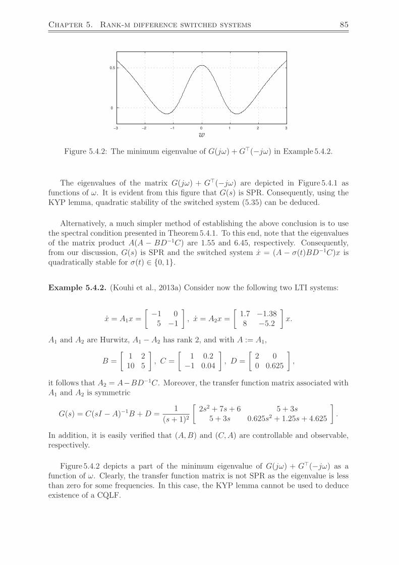
Chapter 5. Rank-m difference switched systems 85
−3 −2 −1 0 1 2 3
0
0.5
w
Figure 5.4.2: The minimum eigenvalue of G(jω) +G(−jω) in Example 5.4.2.
The eigenvalues of the matrix G(jω) + G(−jω) are depicted in Figure 5.4.1 asfunctions of ω. It is evident from this figure that G(s) is SPR. Consequently, using theKYP lemma, quadratic stability of the switched system (5.35) can be deduced.
Alternatively, a much simpler method of establishing the above conclusion is to usethe spectral condition presented in Theorem5.4.1. To this end, note that the eigenvaluesof the matrix product A(A − BD−1C) are 1.55 and 6.45, respectively. Consequently,from our discussion, G(s) is SPR and the switched system x = (A − σ(t)BD−1C)x isquadratically stable for σ(t) ∈ 0, 1.
Example 5.4.2. (Kouhi et al., 2013a) Consider now the following two LTI systems:
x = A1x =
[ −1 05 −1
], x = A2x =
[1.7 −1.388 −5.2
]x.
A1 and A2 are Hurwitz, A1 − A2 has rank 2, and with A := A1,
B =
[1 210 5
], C =
[1 0.2
−1 0.04
], D =
[2 00 0.625
],
it follows that A2 = A−BD−1C. Moreover, the transfer function matrix associated withA1 and A2 is symmetric
G(s) = C(sI − A)−1B +D =1
(s+ 1)2
[2s2 + 7s+ 6 5 + 3s
5 + 3s 0.625s2 + 1.25s+ 4.625
].
In addition, it is easily verified that (A,B) and (C,A) are controllable and observable,respectively.
Figure 5.4.2 depicts a part of the minimum eigenvalue of G(jω) + G(−jω) as afunction of ω. Clearly, the transfer function matrix is not SPR as the eigenvalue is lessthan zero for some frequencies. In this case, the KYP lemma cannot be used to deduceexistence of a CQLF.
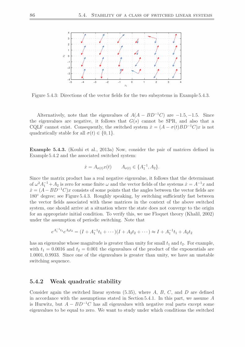
86 5.4. Stability of a class of switched linear systems
−5 −4 −3 −2 −1 0 1 2 3 4
−4
−3
−2
−1
0
1
2
3
4
x1
x 2
Figure 5.4.3: Directions of the vector fields for the two subsystems in Example 5.4.3.
Alternatively, note that the eigenvalues of A(A − BD−1C) are −1.5,−1.5. Sincethe eigenvalues are negative, it follows that G(s) cannot be SPR, and also that aCQLF cannot exist. Consequently, the switched system x = (A − σ(t)BD−1C)x is notquadratically stable for all σ(t) ∈ 0, 1.
Example 5.4.3. (Kouhi et al., 2013a) Now, consider the pair of matrices defined inExample 5.4.2 and the associated switched system:
x = Aσ(t)x(t) Aσ(t) ∈ A−11 , A2.
Since the matrix product has a real negative eigenvalue, it follows that the determinantof ω2A−1
1 +A2 is zero for some finite ω and the vector fields of the systems x = A−1x andx = (A−BD−1C)x consists of some points that the angles between the vector fields are180 degree; see Figure 5.4.3. Roughly speaking, by switching sufficiently fast betweenthe vector fields associated with these matrices in the context of the above switchedsystem, one should arrive at a situation where the state does not converge to the originfor an appropriate initial condition. To verify this, we use Floquet theory (Khalil, 2002)under the assumption of periodic switching. Note that
eA−11 t1eA2t2 = (I + A−1
1 t1 + · · · )(I + A2t2 + · · · ) ≈ I + A−11 t1 + A2t2
has an eigenvalue whose magnitude is greater than unity for small t1 and t2. For example,with t1 = 0.0016 and t2 = 0.001 the eigenvalues of the product of the exponentials are1.0001, 0.9933. Since one of the eigenvalues is greater than unity, we have an unstableswitching sequence.
5.4.2 Weak quadratic stability
Consider again the switched linear system (5.35), where A, B, C, and D are definedin accordance with the assumptions stated in Section 5.4.1. In this part, we assume Ais Hurwitz, but A − BD−1C has all eigenvalues with negative real parts except someeigenvalues to be equal to zero. We want to study under which conditions the switched
Chapter 5. Rank-m difference switched systems 87
system (5.35) possesses a weak CQLF in the sense that there exists a function V (x) =x>Px with P = P> > 0, such that
A>P + PA < 0, (5.45)
(A−BD−1C)>P + P (A−BD−1C) ≤ 0. (5.46)
If such a CQLF exists, then all solutions of the switched system (5.35) are bounded.For this problem we cannot directly exploit Theorem 5.4.1 due to the existence of theequality sign in (5.46). In the next lemma we demonstrate that if (5.45) and (5.46) hold,then A − BD−1C can have at most m eigenvalues equal to zero without having anygeneralized eigenvector. In addition, A−BD−1C cannot have any eigenvalue on the jωaxis for ω 6= 0 provided that G(jω) = C(jωI − A)−1B +D is symmetric for all ω ∈ R.
Lemma 5.4.1. (Kouhi et al., 2014) If (5.45) and (5.46) for a symmetric positivedefinite P hold, G(s) = C(sI − A)−1B + D is symmetric, A is Hurwitz, and D ispositive definite, then A − BD−1C cannot have any eigenvalue on the jω axis forω ∈ R\0. Moreover, A− BD−1C can have at most m eigenvalues equal to 0, and allzero eigenvalues must have linearly independent eigenvectors.
Proof: Suppose A−BD−1C has a non-zero eigenvalue on the jω axis, that is, there existsan eigenvalue jω1 with ω1 6= 0. Note that A being Hurwitz implies det(jω1I − A) 6= 0,and D > 0 implies det(D−1) 6= 0. Then, we have
det(jω1I − (A−BD−1C)
)= 0
⇒ det (jω1I − A) det(I + (jω1I − A)−1BD−1C
)= 0
⇒ det(D−1)det(D + C(jω1I − A)−1B
)= 0
⇒ det(D + C(jω1I − A)−1B
)= 0, (5.47)
which implies that the matrix G(jω1) is singular. Let’s denote the complex eigenvectorcorresponding to eigenvalue 0 of G(jω1) by v ∈ Cm. Similarly, we can show that thematrix G(−jω1) = G>(−jω1) = G∗(jω1) is also singular and has a left eigenvector v∗
corresponding to the eigenvalue 0. Thus, recalling Lemma 5.2.4, the following holds:
1
2v∗[G(jω1) +G>(−jω1)]v =
= v∗[D − C(ω21I + A2)−1AB]v = 0. (5.48)
On the other hand, similar to the situation discussed in the proof of necessity inTheorem 5.3.1, a necessary condition for (5.45) and (5.46) to hold is that the ma-trix ω2A−1 + (A − BD−1C) for ω 6= 0 is non-singular. Hence, by continuity ofdet(ω2I + A(A − BD−1C)) with respect to ω and the fact that det(ω2I + A2) > 0,we can deduce
det(ω2I + A(A−BD−1C)
)> 0
⇒ det(ω2I + A2
)det(D − C(ω2I + A2)−1AB) > 0
⇒ det
(1
2G(jω) +G>(−jω)
)> 0.
88 5.4. Stability of a class of switched linear systems
Now, continuity of the determinant with respect to ω indicates that G(jω) + G>(−jω)is positive definite for all ω ∈ R\0, in particular for ω = ω1. However, this is acontradiction with (5.48).
Now, we prove A−BD−1C can have at most m eigenvalues equal to 0. This proof issimilar to the proof given in Shorten et al. (2009). Since the inequality (5.46) holds, thesystem x = (A−BD−1C)x is stable, that is, the algebraic multiplicity and geometric mul-tiplicity of the zero eigenvalues are the same. Now, suppose that we have more thanm lin-early independent eigenvectors corresponding to zero eigenvalues. Let us define the func-tions g1(x) = x>(A>P +PA)x and g2(x) = x>
((A−BD−1C)>P + P (A−BD−1C)
)x.
Obviously, at least for n−m linearly independent vectors vi ∈ Rn with i ∈ 1, . . . , n−m,we have g1(vi) = g2(vi), for instance, for those vi’s that satisfy v>i PB = 0. Suppose thereare more than m linearly independent vectors x such that g2(x) is zero. Then, the twospaces x : g2(x) = 0 and x : g2(x) = g1(x) intersect at least at one non-zero point,implying that there exists a non-zero vector x such that
g1(x) = g2(x) = 0.
The condition g1(x) = 0 is in contradiction with the choice of P in (5.45).
Now, the following theorem provides sufficient and necessary conditions for theexistence of a weak CQLF for the switched system (5.35).
Theorem 5.4.2. (Kouhi et al., 2014) Assume A is Hurwitz and all eigenvalues of thematrix A − BD−1C have negative real parts or are zero. Furthermore, assume that thezero eigenvalue has a multiplicity of m− p, and associated with the zero eigenvalue is afull set of m− p linearly independent eigenvectors. Suppose also that
CAiB = (CAiB)> ∀i ∈ 0, 1, . . . , n− 1, (5.49)
D = D> > 0, (A,B) is controllable, and (C,A) is observable. Then, the switched system(5.35) is weakly quadratically stable if and only if A(A − BD−1C) has no real negativeeigenvalue and has exactly m− p eigenvalues equal to zero.
Proof of sufficiency: Recall that Lemma 5.2.1 implies that the symmetry conditions(5.49) and D = D> suffice for the transfer function matrix G(s) = C(sI − A)−1B + Dto be symmetric. The remainder of the proof of sufficiency consists of two parts. InPart A, we prove that G(0) ≥ 0 and rank(G(0)) = p. Afterwards, in Part B we useG(1
s) in combination with the KYP lemma to complete the proof of sufficiency.
Part A: Following the proof of sufficiency in Theorem 5.3.1, A(A−BD−1C) having noreal negative eigenvalue implies that
det(ω2I+A(A−BD−1C)) > 0
⇒ det(D − C(ω2I + A2)−1AB) > 0 ∀ω ∈ R \0. (5.50)

Chapter 5. Rank-m difference switched systems 89
Therefore, analogous to the proof of sufficiency in Theorem 5.3.1, we can argue that
1
2G(jω) +G>(−jω) = D − C(ω2I + A2)−1AB > 0 ∀ω ∈ R \0.
By continuity of the eigenvalues with respect to ω around zero, we conclude that thematrix
G(0) = limω→0
1
2G(jω) +G>(−jω) = D − CA−1B
does not have any eigenvalue in the open left half plane, that is, G(0) = D−CA−1B ≥ 0.Next, we prove that G(0) has exactly m − p eigenvalues equal to zero. To this end,consider the equality
(A−BD−1C)A−1B = BD−1(D − CA−1B),
then exploiting the Sylvester rank inequality (see Appendix A.2.5.1 and Horn and John-son (1990)), we have
rank(BD−1(D − CA−1B)
)= rank
((A−BD−1C)A−1B
)≥
rank(A−BD−1C) + rank(A−1B)− n =
[n− (m− p)] +m− n = p.
As rank(BD−1) = m ≥ p, we must have rank(D − CA−1B) ≥ p. On the other hand,A− BD−1C has exactly m− p eigenvalues equal to zero with a full set of eigenvectors,so there exists a matrix W> ∈ R(m−p)×n constructed from the left eigenvectors of A −BD−1C corresponding to the zero eigenvalue, such that W>(A − BD−1C) = 0. Notethat rank(W>BD−1) = m − p since W>A has full rank and W>A = W>BD−1C. Itthus follows from
W>(A−BD−1C)A−1B = 0⇒W>BD−1(D − CA−1B) = 0 (5.51)
that the columns of D−1B>W ∈ Cm×(m−p) are indeed left eigenvectors of G(0) =D − CA−1B corresponding to the zero eigenvalues. Note also that the symmetry ofG(0) excludes the possibility of the existence of any generalized eigenvector for G(0).Consequently, as rank of G(0) ≥ p and (5.51) holds, we have rank(D − CA−1B) = p,indicating that this matrix has exactly m− p zero eigenvalues.
Part B: Define the system G(s) := G(1s) = C(sI − A)−1B + D, with the state space
representation (A, B, C, D),
A = A−1, B = −A−1B, C = CA−1, D = D − CA−1B.
Consequently, the symmetry of G(s) follows from symmetry of G(s). On the other hand,(A, B) and (C, A) by construction are controllable and observable, respectively, and thematrix D ≥ 0 has rank p. Now, Theorem 5.3.2 implies that A(A − BD−1C) havingno real negative and exactly m − p zero eigenvalues, is equivalent to G(s) being SPR.Then, the Kalman-Yakubovic-Popov lemma (see Zhou et al. (1996) and Appendix A.4.1)implies that there exist a scalar α > 0 and matrices P = P> > 0, L, and W such that
A>P + PA = −L>L− αP, (5.52)
B>P +W>L = C, (5.53)
D + D> = W>W. (5.54)
90 5.4. Stability of a class of switched linear systems
The first equation in (5.52) ensures that
A−>P + PA−1 < 0. (5.55)
By pre- and post-multiplying of this equation by A> and A, respectively, we get A>P +PA < 0 , which verifies that (5.45) holds. Next, we show that (5.46) also holds. To thisend, first we claim that [
A−>P + PA−1 PB − C>B>P − C −(D + D>)
]≤ 0. (5.56)
Note that D ≥ 0 and we shall demonstrate that the Schur complement of the abovematrix is less than or equal to zero (see Appendix A.2.2), in other words,
S = −(D + D>)− (B>P − C)(A−>P + PA−1)−1(PB − C>) ≤ 0.
Using equations (5.52-5.54), we get
S = −(D + D>)− (B>P − C)(A−>P + PA−1)−1(PB − C>)
= −W>W +W>L (αP + L>L)−1L>W =
= −W> [I − L(αP + L>L)−1L>]W. (5.57)
In (5.57), the matrix I − L(αP + L>L)−1L> is the Schur complement of the positivedefinite matrix [
αP + L>L L>
L I
]with respect to the upper left block, which is also positive definite and subsequentlyS < 0. Now, let reformulate (5.56) as[
A−1 B−C −D
]> [P 00 I
]+[
P 00 I
] [A−1 B−C −D
]≤ 0. (5.58)
Since D − CAB = D, we have[A−1 B−C −D
]−1
=[A− AB(−D + CAB)−1CA −AB(−D + CAB)−1
(−D + CAB)−1CA (−D + CAB)−1
]=
[A−BD−1C −BD−1
−D−1C −D−1
]; (5.59)
see Appendix A.2.1. By pre-multiplying the inequality (5.58) by the transpose of theabove matrix and by post-multiplying by the above matrix itself, we end up with[
(A−BD−1C)>P + P (A−BD−1C) −(PB + C>)D−1
−D−1(B>P + C) −2D−1
]≤ 0,
Chapter 5. Rank-m difference switched systems 91
from which it immediately follows that
(A−BD−1C)>P + P (A−BD−1C) ≤ 0. (5.60)
Thus, we can say that V (x) = x>Px is a weak Lyapunov function for both x = Ax andx = (A−BD−1C)x. This establishes the proof of sufficiency.
Proof of necessity: The proof of the fact that A(A − BD−1C) does not haveany non-zero real negative eigenvalue is similar to the proof of necessity given inTheorem 5.4.1.
The last part of the proof is concerned with proving that the product AA2, withA2 = A−BD−1C, has exactly m− p zero eigenvalues equal to zero. To show this holds,first notice that AA2 has exactly m − p zero eigenvalues with a full set of eigenvectors.This fact can be derived by considering that
rank(AA2) = rank(A2).
Therefore, if AA2 has more than m − p zero eigenvalues, then it must contain at leastone generalized eigenvector, say v2 ∈ Rn satisfying AA2v2 = v1, and AA2v1 = 0; seeAppendix A.2.7. This implies that
A2v2 = A−1v1, and A2v1 = 0. (5.61)
Moreover, it can be inferred from the inequality A−>P + PA−1 < 0 that the functionf(x) = x>(A−>P + PA−1)x is always negative for all non-zero x ∈ Rn, in particular forx = v1. Recalling (5.61), we have
v>1 (A−>P + PA−1)v1 < 0
⇒ v>2 A>2 Pv1 + v>1 PA2v2 < 0. (5.62)
On the other hand, with regard to (5.46) the inequality g(x) = x>(A>2 P + PA2)x ≤ 0must hold for all x ∈ Rn. Now, choosing x = βv1 + v2 with β ∈ R as a parameter andconsidering A2v1 = 0, we should have
(βv1 + v2)>(A>2 P + PA2)(βv1 + v2) ≤ 0
⇒ β(v>2 A>2 Pv1 + v>1 PA2v2) + v>2 (A>2 P + PA2)v2 ≤ 0. (5.63)
As the inequalities e = v>2 A>2 Pv1 + v>1 PA2v2 < 0 and g(v2) = v>2 (A>2 P + PA2)v2 ≤ 0
both hold, there exists always a β ∈ R which makes the expression βe + g(v2) positive.For instance, one can choose β < −g(v2)/e. However, this is evidently in contradictionwith (5.63).
Example 5.4.4. (Kouhi et al., 2014) Consider two matrices
A1 =
[−1 0
5 −1
], A2 =
[0 −10 −5
].
92 5.4. Stability of a class of switched linear systems
A1 is Hurwitz and A2 has all eigenvalues in the open left half plane except one eigenvalueat zero. In addition A1 − A2 has rank two, and with A = A1
B =
[1 2
10 5
], C =
[1 0.2−1 0.4
], D =
[1 00 1
],
we have A2 = A−BD−1C. Furthermore, the transfer function matrix
G(s) = C(sI − A)−1B +D =1
(s+ 1)2
[s2 + 5s+ 5 3s+ 5
3s+ 5 s2 + 2s+ 5
]
is symmetric. Note that (A,B) and (C,A) are controllable and observable, respectively.The eigenvalues of the matrix A1A2 are 0, 0 indicating that there is no weak CQLF forthe switched system associated with the two matrices A1 and A2.
Example 5.4.5. (Kouhi et al., 2014) Consider two matrices
A1 =
[−0.9 −0.1
4.5 −1.4
], A2 =
[0 −10 −5
].
A1 is Hurwitz and A2 has all eigenvalues in the open left half plane except one eigenvalueat zero. In addition A1 − A2 has rank two, and with A = A1,
B =
[0.9 1.89 4.5
], C =
[1 0.2−1 0.4
], D =
[1 00 1
],
we have A2 = A−BD−1C. Furthermore, the transfer function matrix
G(s) = C(sI − A)−1B +D =1
s2 + 2.3s+ 1.71
[s2 + 5s+ 4.5 2.7s+ 4.5
2.7s+ 4.5 s2 + 2.3s+ 4.5
]
is symmetric. Note that (A,B) and (C,A) are controllable and observable, respectively.The eigenvalues of the matrix A1A2 are 0, 2.5, implying that there is a weak CQLFV (x) = x>Px for the switched system (5.35). For instance, one can choose
P =
[1.48 −0.296−0.296 0.3089
].
Example 5.4.6. (Kouhi et al., 2014) Consider the switched electrical circuit illustratedin Figure 5.4.4. The variables v1(t) and v2(t) are voltages of two capacitors with capacitiesC1 and C2, respectively. Let x(t) := [v1(t) v2(t)]> indicate the vector of the systemstates. Depending on the status of the switch S, the system model can be representedby a switched linear system with two modes x = Aix for i ∈ 1, 2, where
A1 =
−1R1C1
1R1C1
1R1C2
−(R1+R2)R1R2
1C2
, A2 =
0 0
0 −1R2C2
. (5.64)
Chapter 5. Rank-m difference switched systems 93
R1
R2
C1
v1(t)
C2
v2(t)
S
Figure 5.4.4: A switched electrical circuit.
In (5.64) A1 refers to the situation when S is closed and A2 refers to the conditionwhen S is open. Note that A1 is Hurwitz and A2 is singular including exactly one zeroeigenvalue and one real negative eigenvalue. In addition, A1 and A2 have rank onedifference. Defining A := A1, B := [−1/C1 1/C2]
, C := [1/R1 −1/R1], and D := I, wehave A2 = A−BD−1C and the transfer function G(s) = C(sI −A)−1B +D is triviallysymmetric. Furthermore, (A,B) and (C,A) are controllable and observable, respectively.Now, consider that the matrix
A1A2 =
⎡⎢⎣ 0 −1
R1R2C1C2
0 (R1+R2)
R1R22C
22
⎤⎥⎦
has no real negative eigenvalue and has exactly one zero eigenvalue. Hence, accordingto Theorem5.4.2 this electrical circuit is weakly quadratically stable, implying that thevoltages of both capacitors remain bounded in spite of all possible switching events andeach initial condition.
5.5 Stabilization of controlled switched linear sys-
tems
In this part, we employ the theory elaborated for stability of switched systems associatedwith symmetric transfer functions, for stabilization of controlled switched linear systems.We consider the problem of stabilization of a class of switched linear systems defined by
x = Ax+ σ(t)Bu σ(t) ∈ 0, 1, (5.65)
where A ∈ Rn×n is a Hurwitz matrix, B ∈ R
n×m, and the pair (A,B) is controllable. Thegoal is to find a set of feedback controls in the form of u = Kx, such that the switchedsystem
x = (A+ σ(t)BK)x σ(t) ∈ 0, 1, (5.66)
is quadratically stable, that is, there exists a matrix P = P > 0 such that
(A+ σ(t)BK)P + P (A+ σ(t)BK) < 0 σ(t) ∈ 0, 1. (5.67)
94 5.5. Stabilization of controlled switched linear systems
For this purpose, we suppose K has a structure of the form K = −D−1C. This modifies(5.66) into the form
x = (A− σ(t)BD−1C)x σ(t) ∈ 0, 1. (5.68)
Now, our wish is to design the unknown matrices D and C by utilizing Theorem 5.4.1.To this end, we require D = D> > 0, and the transfer function matrix G(s) = C(sI −A)−1B + D to be symmetric and to be strictly positive real. Referring to Lemma 5.2.2the transfer function G(s) is symmetric and has the minimal state space realization(A,B,C,D) if and only if there exists a non-singular matrix S = S> such that
A>S = SA, B>S = C, and D = D>. (5.69)
Therefore, defining Y = S−1, the matrix A satisfies the following Sylvester equation
AY − Y A> = 0. (5.70)
For finding a solution of this equation, similar to the proof of Lemma 5.2.3we use the Kronecker product and the vectorization operator vec(Y ) =[y11 . . . yn1 y12 . . . yn2 . . . y1n . . . ynn]>. We can then reformulate (5.70) in the form of
(In ⊗ A− A⊗ In) vec(Y ) = 0. (5.71)
Define S := Y −1 and C := B>S. As (A,B) is controllable, (C,A) is also observable.Furthermore, we must have G(jω) +G>(−jω) > 0. This is equivalent to the condition
1
2G(jω) +G>(−jω) = D − C(ω2I + A2)−1AB > 0. (5.72)
Therefore, a sufficient condition for the last equation to hold is that
D >(supω σmax
(C(ω2I + A2)−1AB
)).Im. (5.73)
Note that C(ω2I + A2)−1AB is finite as ω2I + A2 is always non-singular, andlimω→∞C(ω2I + A2)−1AB = 0. Consequently, the right hand side of the inequal-ity (5.73) is always finite. This verifies that there exists infinitely many matricesD = D> > 0 such that the inequality (5.73) holds true. This shows that the switchedsystem (5.66) is always quadratically stabilizable.
In a different context using a distinct approach, output feedback design for an LTIsystem has been introduced for making the closed loop system to be SPR (Huang et al.,1999).
Remark 5.5.1. Assume a Hurwitz matrix A is given. One advantage of using thediscussed approach is to specify a set of matrices A2 which differ by a rank-m matrixand share a common Lyapunov solution with A.
Example 5.5.1. Suppose we want to find a set of feedbacks u = Kx, where K ∈ R2×2,which stabilizes the switched linear system (5.66) with the data
A =
[−0.9 −0.1
4.5 −1.4
], B =
[0.9 1.8
9 4.5
].

Chapter 5. Rank-m difference switched systems 95
Note that A is Hurwitz and (A,B) is controllable. Now, a matrix S satisfying A>S −SA = 0 equals
S =
[−0.0025 0.7049
0.7049 −0.0783
].
This allows us to compute C as
C = B>S =
[6.3422 −0.073.1677 0.9167
].
Now, we derive an appropriate matrix D with regard to (5.73). Computingsupω σmax (C(ω2I + A2)−1AB) = 28.41, we can pick D as any two dimensional sym-metric positive matrix whose minimum eigenvalue is greater than 28.41. For instance,we can choose
D =
[30 00 40
].
Then, the resulting state feedback gain and the closed loop matrix are
K = −D−1C =
[−0.2114 0.0023−0.0792 −0.0229
], and A−BD−1C =
[−1.2328 −0.1392
2.2410 −1.4821
].
The eigenvalues of A(A − BD−1C) are equal to 1.170 ± 1.515i, which confirms that aCQLF V (x) = x>Px for the switched linear system (5.66) exists. Using the MATLABLMI Toolbox one such P can be computed as
P =
[5.6408 −1.2073−1.2073 1.4448
].
5.6 Conclusions
In this chapter, we explored conditions under which a symmetric transfer function matrixcan be associated with a given pair of Hurwitz matrices. Furthermore, we showed thatif the symmetric transfer function matrix associated with this pair is strictly positivereal, then a common Lyapunov solution for such pair of matrices exists. On this basis,we introduced an approach for stabilization of a class of switched linear systems whoseconstituent matrices differ by a rank m matrix. In the case that one matrix is Hurwitz,and the other one has all eigenvalues with negative real parts and some eigenvalues equalto zero, we extended our result in terms of a weak common quadratic Lyapunov function.

96 5.6. Conclusions

Chapter 6. Control of hybrid linear systems 97
Chapter 6
Control of hybrid linear systems
6.1 Introduction
In this chapter, we investigate control of hybrid linear systems including linear flowand jump dynamics. We start with stability of such hybrid systems and establisha link between their stability and stability of switched linear systems discussed inthe previous chapters. Moreover, we derive convenient conditions for robust sta-bility of such hybrid systems. It turns out that the concept of stability for hybridlinear systems is very similar to the concept of stability for switched linear systems.In addition, we study some problems concerning optimal control of hybrid linear systems.
In the first optimal control problem in Section 6.4, we find analytic expressionsfor lower and upper bounds of the optimal value of the cost function for a linearquadratic problem in a class of hybrid linear systems. The optimization probleminvolves state space constraints and switches between the continuous evolution andjumps at fixed time instances on the boundaries of flow and jump sets. The basicidea for our approach uses analytical solutions to continuous- and discrete-time LQRproblems with fixed initial and final states over fixed time intervals; see, for instance,Lewis and Syrmos (1995); Bryson and Ho (1975). We show that the optimal cost ofeach time interval can be represented by its initial and final state variables. Using thisfact, we propose a parameterization method with states corresponding to the initialand end points of each generalized time domain as decision variables, and show thatwe can reformulate the problem as a static optimization problem. The lower bound forthe optimal value of the cost function can be computed analytically, whereas the upperbound can be computed numerically via solving a quadratic programming problem.Throughout Section 6.4, we use the restrictive assumption that switching times are fixed.
Therefore, in Section 6.5, we tackle a free switching times optimal control problem fora class of hybrid linear systems. We employ the same approach as the one for the fixedswitching times optimal control problem to describe the switching points with respectto switching time instances. Moreover, we show that the problem of finding switchingtime instances gives rise to solving a differential algebraic equation with given boundaryconditions. The resulting problem, of course, can only be solved numerically.
98 6.2. Stability of a class of hybrid linear systems
6.2 Stability of hybrid linear systems with single
flow and jump dynamics
Consider a simple form of hybrid linear systems consisting of a single flow and a jumpdynamics given by
H :
x = Ax x ∈ C,x+ = Gx x ∈ D, (6.1)
where the sets C ⊆ Rn and D ⊆ Rn denote the flow and jump sets, respectively.In general, C and D can be open or closed sets, but in this section we assume bothare closed. Furthermore, we assume C,D ⊆ Rn, C ∪ D = Rn, A is Hurwitz, and alleigenvalues of G are inside the unit circle.
Given a number K ∈ N0 := N ∪ 0, the domain of x for such a system is a subsetof R≥0 × N0 defined by time instances
0 := t0 ≤ t1 ≤ t2 . . . ≤ tK , (6.2)
as follows:
TK :=K−1⋃k=0
Tk,
where
Tk := [tk, tk+1]× k ∀k ∈ 0, . . . , K − 1. (6.3)
This time domain is called “hybrid time domain”; see, e.g., Goebel et al. (2012). Notethat in (6.2) K and tK are allowed to go beyond all bounds.
Given a number K ∈ N0 and x0 := x(t0, 0) ∈ C ∪ D, we say x : TK → Rn is asolution of the system (6.1) if
a) for each (t, k) ∈ Tk where (tk, tk+1) has nonempty interior and x(t, k) ∈ C, thederivative of x(t, k) with respect to t is defined and the following differential equa-tion holds
d
dtx(t, k) = Ax(t, k) ∀t ∈ (tk, tk+1).
b) for each (t, k) ∈ TK such that (t, k + 1) ∈ TK , and x(tk, k) ∈ D, the followingdifference equation holds
x(tk+1, k + 1) = Gx(tk+1, k).
Note that from item a) in this definition, one can realize that the mapping(t, k) 7→ x(t, k) is absolutely continuous within any interval Tk with nonempty interior.
We say the hybrid system H is quadratically stable if a quadratic function V (x) =x>Px with P = P> > 0 exists such that
A>P + PA < 0, (6.4)
G>PG− P < 0. (6.5)
Chapter 6. Control of hybrid linear systems 99
Analogous to the concept of stability for switched linear systems, one would expect ifsuch a P exists, exponential stability of the system (6.1) is implied. We now give a shortproof for this argument. Without loss of generality assume that x(t, k) ∈ C for some(t, k) ∈ Tk . For exponential stability there must exist numbers α, β > 0 such that
‖x(t, k)‖ ≤ αe−β(t+k−t0)x(t0, 0). (6.6)
We show now that (6.6) holds. If both (6.4) and (6.5) hold, there exists a number0 < γ < λmax(P ), such that
A>P + PA < −γI,G>PG− P < −γI.
This implies that for each (t, k) ∈ Tk, and x ∈ C
V (x) = x>(A>P + PA)x ≤ −γ‖x‖2. (6.7)
As P is symmetric positive definite, we can write
λmin(P )‖x‖2 ≤ x>Px = V (x) ≤ λmax(P )‖x‖2. (6.8)
Therefore, defining γc := γ/λmax(P ), (6.7) gives us the following upper bound for V :
V (x) =x>(A>P + PA)x ≤ −γ‖x‖2 ≤ −γλmax(P )
V (x)
⇒ V (x(t, j)) ≤ V (x(t− tj, j))e−γc(t−tj) ∀(t, j) ∈ Tj, j ≤ k. (6.9)
On the other hand, for each (t, j) ∈ TK , such that x(t, j + 1) ∈ TK and x(t, j) ∈ D forsome j ≤ k, we have
V (x(t, j + 1))− V (x(t, j)) = x>(G>PG−G)x ≤ −γ‖x(t, j)‖2.
Again, recalling (6.8) we can write
−γ‖x(t, j)‖2 ≤ −γV (x(t, j))
λmax(P )∀(t, j) ∈ TK .
Now, defining γd := −ln (1− γ/λmax(P )) > 0, we have
V (x(t, j + 1))− V (x(t, j)) ≤ − γ
λmax(P )V (x(t, j))
⇒ V (x(t, j + 1)) ≤(
1− γ
λmax(P )
)V (x(t, j))
⇒ V (x(t, j + 1)) ≤ e−γdV (x(t, j)) ∀(t, j), (t, j + 1) ∈ TK , j < k. (6.10)
As a result, combining (6.9) and (6.10), we get
V (x(t, k)) ≤ V (x(t0, 0))e−[γc(t−t0)+γdk]. (6.11)

100 6.2. Stability of a class of hybrid linear systems
Now, considering (6.8) and defining β := min(γc, γd), we can write
‖x(t, k)‖2 ≤ V (x(t0, 0))
λmin(P )e−β(t−t0+k) ∀(t, k) ∈ TK . (6.12)
This immediately implies exponential stability of the hybrid linear system (6.1). For suchreason, finding a convenient condition under which a CQLF for this system exists is ourpoint of interest. Note that (6.4) and (6.5) represent continuous and discrete Lyapunovinequalities, respectively. Nevertheless, we can use bilinear transformation as proposedin Mason and Shorten (2004) to unify the two inequalities in the form of continuousLyapunov inequalities.
Lemma 6.2.1. Let all eigenvalues of G be inside the unit circle. Then, P = P> > 0 isa solution of the discrete Lyapunov equation
G>PG− P = −Qd with Qd > 0, (6.13)
if and only if P is the solution of the following continuous Lyapunov equation
C(G)>P + P C(G) = −Qd, (6.14)
where
C(G) = (G− I)(G+ I)−1, and Qd = 2(G+ I)−>Qd(G+ I)−1 > 0.
The mapping G 7→ C(G) = (G − I)(G + I)−1 is known as the bilinear transformation;see Mason and Shorten (2004).
Proof of sufficiency: Note that (6.14) is equivalent to
(G+ I)−>(G− I)>P + P (G− I)(G+ I)−1 = −2(G+ I)−>Qd(G+ I)−1. (6.15)
By pre- multiplying (6.15) by (G+ I)> and post- multiplying it by (G+ I), we deduce
(G− I)>P (G+ I) + (G+ I)>P (G− I) = −2Qd. (6.16)
Thus, after simplification (6.13) results. Due to simplicity, proof of necessity is notgiven.
Lemma 6.2.1 indicates that for checking the existence of a CQLF for the hybridlinear system (6.1), it is necessary and sufficient to consider the common Lyapunovsolution existence problem for the matrix pair (A,C(G)). This problem was extensivelydiscussed in Chapters 4 and 5, on stabilization and stability problems for switched linearsystems.

Chapter 6. Control of hybrid linear systems 101
6.3 Robust Stability of hybrid linear systems
Assume A is Hurwitz and all eigenvalues of G are inside the unit circle. We define thefollowing concept of robust stability for the hybrid linear system (6.1).
Definition 6.3.1. (See Appendix A.7, Cai et al. (2007); Goebel et al. (2012)) A smoothfunction V (x) is a robust Lyapunov function for the hybrid linear system (6.1), if thereexist two increasing positive definite functions α1, α2 : [0,∞)→ [0,∞) satisfying
α1(‖x‖) ≤ V (x) ≤ α2(‖x‖), (6.17)
〈∇V (x), Ax〉 ≤ −V (x) ∀x ∈ C, (6.18)
V (Gx) ≤ e−1V (x) ∀x ∈ D. (6.19)
Now, the following definition of robustness of the hybrid linear system (6.1) is adoptedfrom the general definition of robustness for hybrid systems introduced, for example, byCai et al. (2007); Goebel et al. (2012).
Definition 6.3.2. (See Appendix A.7 and Cai et al. (2007); Goebel et al. (2012)) Thehybrid linear system (6.1) is said to be robustly asymptotically stable if a continuousperturbation function δ : Rn → Rn
≥0 with δ(x) > 0 for x ∈ Rn\0 exists, such that theperturbed hybrid system given by the differential and difference inclusions
Hδ :=
x ∈ Fδ(x) x ∈ Cδ,x+ ∈ Gδ(x) x ∈ Dδ,
(6.20)
with
Cδ := x : (x+ δ(x)B) ∩ C 6= ∅,Fδ(x) := A. ((x+ δ(x)B) ∩ C) + δ(x)B ∀x ∈ Cδ,Dδ := x : (x+ δ(x)B) ∩D 6= ∅,Gδ(x) := v : v ∈ g + δ(g)B, g ∈ G. ((x+ δ(x)B) ∩D) ∀ x ∈ Dδ, (6.21)
is asymptotically stable, where B denotes the closed unit ball in Rn.
From the results by Cai et al. (2007); Goebel et al. (2012), robust asymptotic stabilityof the hybrid linear system (6.1) is equivalent to the existence of a robust Lyapunovfunction; see Theorem A.7.2 in Appendix A. Now, we study the robust stability problemfor the hybrid linear system (6.1) when the robust Lyapunov function is quadratic, thatis, there exist V (x) = x>Px with P = P> > 0 such that (6.18-6.19) hold. Note thatcondition (6.17) does not limit the selection of such a Lyapunov function. Indeed, forany P = P> > 0, two appropriate functions α1 and α2 exist. For instance, one can take
α1(‖x‖) = λmin(P )‖x‖2, α2(‖x‖) = λmax(P )‖x‖2,
102 6.3. Robust Stability of hybrid linear systems
where λmin(P ) and λmax(P ) denote the minimum and maximum eigenvalues of P , re-spectively. Now, (6.18-6.19) can be rewritten as
A>P + PA+ P ≤ 0, (6.22)
G>PG− P + (1− e−1)P ≤ 0. (6.23)
It follows from (6.22-6.23) that the matrix(A+ 1
2I)
does not have any eigenvalue in
the open right half plane, and all eigenvalues of (e12G) lie within the closed unit disc.
Therefore, intuitively one may expect that the system (6.1) exhibits robustness propertiesin the presence of some bounded uncertainties. To verify this formally, we introduce aLipschitz uncertainty function in the form of δ(x) = ψ‖x‖. Then, (6.21) becomes:
Cδ := x : (x+ ψ‖x‖.B) ∩ C 6= ∅, (6.24)
Fδ(x) := A((x+ ψ‖x‖.B) ∩ C) + ψ‖x‖.B ∀ x ∈ Cδ, (6.25)
Dδ := x : (x+ ψ‖x‖.B) ∩D 6= ∅, (6.26)
Gδ(x) := v : v ∈ g + ψ.‖g‖.B, g ∈ G. ((x+ ψ.‖x‖B) ∩D) ∀ x ∈ Dδ. (6.27)
In the following lemma we introduce an upper bound for such a function δ(x) bytaking into account that the perturbed system Hδ should be asymptotically stable.In addition, we show that the perturbed hybrid system is exponentially stable. Notethat our approach for the proof of this lemma is different from the one used inCai et al. (2007); Goebel et al. (2012) for general nonlinear differential/difference in-clusions. We exploit some characteristics of systems with linear flow and jump dynamics.
Lemma 6.3.1. Suppose there exists a function V (x) = x>Px with P = P> > 0 satisfy-ing (6.22−6.23). Then, the perturbed hybrid system Hδ defined by (6.20) and (6.24−6.27)is exponentially stable for
δ(x) = ψ.‖x‖ = min(δc(x), δd(x)
), (6.28)
where
δc(x) = ψc.‖x‖,with ψc :=λmin(P )
4 [λmax(P )(2σmax(A) + 3)], (6.29)
δd(x) = ψd.‖x‖,with ψd :=0.02 λmin(P )
3λmax(P )(σmax(G)2 + 2), (6.30)
and λmax(.) and σmax(.) denote the maximum eigenvalue and singular value of a matrix,respectively.
Proof: Our proof consists of three parts. In Part A, we present a proof for continuousdynamics, while in Part B we state a proof for discrete counterpart. Finally, in Part C,we prove exponential stability of the perturbed hybrid system Hδ.
Part A: Define Cδc and Fδc as Cδ and Fδ in (6.24) and (6.25) by setting ψc instead of

Chapter 6. Control of hybrid linear systems 103
ψ. We demonstrate that the derivative of V (x) for all perturbations bounded by δc(x)is negative. In other words, we show for each x 6= 0
maxf∈Fδc (x)
〈∇V (x), f〉 < 0 ∀x ∈ Cδc .
First, note that by definition of Cδc , for any x ∈ Cδc and y ∈ C such that (y−x) ∈ δc(x)B,there exists a v ∈ B satisfying
y = x+ δc(x)v = x+ ψc‖x‖v. (6.31)
On the other hand, by definition of ψc in (6.29), we have 0 < ψc < 1. This means thatthe closest point of the set x ∈ Cδc : x + ψc‖x‖B to the origin is indeed the pointx1 := x(1− ψc). This implies
‖y‖ ≥ (1− ψc)‖x‖, and (1− ψc)‖x‖.B ⊆ ‖y‖.B. (6.32)
Paying attention to (6.32) and (6.31), one can write
x ∈ y + ψc1‖y‖.B, where ψc1 :=ψc
1− ψc. (6.33)
In addition, from (6.32), we can write
‖x‖ ≤ 1
1− ψc‖y‖ ⇒ ψc‖x‖ ≤
ψc1− ψc
‖y‖ = ψc1‖y‖, (6.34)
and also y 6= 0 when x 6= 0. Now, note that referring to (6.25) and (6.33) any vectorinside the set Fδc(x) can be written as
f = Ay + ψc.‖x‖v3 = Ay + ψc1.‖y‖v2, (6.35)
for x ∈ Cδc , y ∈ C, and some v2, v3 ∈ B. Utilizing (6.18), (6.35), and (6.33) the derivativeof the Lyapunov function is bounded by:
maxf∈Fδc (x)
〈∇V (x), f〉 = maxv2∈B, x∈Cδc
〈2x>P,Ay + ψc1.‖y‖v2〉
= maxv1,v2∈B
〈2(y + ψc1.‖y‖.v1)>P , Ay + ψc1.‖y‖v2〉
= y>(A>P + PA)y + 2ψc1.‖y‖.y>Pv2 + 2ψc1.‖y‖.v>1 P.Ay+ 2ψ2
c1.‖y‖2.v>1 Pv2
≤ −y>Py + 2ψc1.‖y‖.‖y‖.‖Pv2‖+ 2ψc1.‖y‖.‖v>1 P‖.‖Ay‖+ 2ψ2
c1.‖y‖2.‖v1‖.‖Pv2‖.
As P is symmetric and positive definite, its maximum eigenvalue equals its maximumsingular value. Thus, ‖Pv1‖ ≤ λmax(P ) and ‖Pv2‖ ≤ λmax(P ) . Moreover, the inequality‖Ay‖ ≤ σmax(A)‖y‖, in general, holds true. By the definition of ψc in (6.29), we havealso ψc ≤ 1
2and therefore, 2ψ2
c1 ≤ ψc1. Furthermore, by the definition of ψc1 from (6.33),we have ψc1 ≤ 2ψc. Consequently, the following upper bound for the derivative of theLyapunov function results
maxf∈Fδc (x)
〈∇V (x), f〉 ≤ −y>Py + 2ψc
(3 + 2σmax(A)
)‖y‖2λmax(P ).
104 6.3. Robust Stability of hybrid linear systems
Substituting ψc from (6.29) into the last equation and having y 6= 0 lead to
maxf∈Fδc (x)
〈∇V (x), f〉 ≤ −y>Py +1
2λmin(P ).‖y‖2 ≤ −1
2y>Py < 0. (6.36)
Part B: Let us define Dδd and Gδd similar to what defined for Dδ and Gδ in (6.26) and(6.27), respectively, by changing the role of δ to δd. We show that during a jump thefollowing Lyapunov inequality holds
maxg∈Gδd(x)
V (g)− V (x) < 0 ∀x ∈ Dδd\0. (6.37)
With the similar argument as presented in Part A, for each x ∈ Dδd and y ∈ D suchthat (x− y) ∈ δd(x)B, there exists a vector v1 ∈ B satisfying
x = y + ψd1.‖y‖v1, where ψd1 =ψd
1− ψd. (6.38)
Notice also any vector g ∈ Gδd , in accordance with (6.27), can be formulated as
g = Gy + ψd.‖Gy‖v2, y ∈ D, ∃v2 ∈ B. (6.39)
Thus, recalling (6.39) we have
maxg∈Gδd (x)
V (g)− V (x) = maxv1,v2∈B
(Gy + ψd.‖Gy‖v2
)>P(Gy + ψd.‖Gy‖v2
)(6.40)
− (y + ψd1.‖y‖v1)>P (y + ψd1.‖y‖v1)
= y>G>PGy − y>Py+ max
v1,v2∈B
(2ψd.‖Gy‖v>2 P.Gy + ψ2
d.‖Gy‖2v>2 Pv2
− 2ψd1.‖y‖v>1 Py − ψ2d1.‖y‖2v>1 Pv1
).
Note that from the definition of ψd in (6.30), we have ψd ≤ 1/2 . Therefore, from thedefinition of ψd1 in (6.38), we can deduce ψd1 ≤ 2ψd ≤ 1. Moreover, the followinginequalities are valid
maxv2∈B
ψd‖Gy‖v>2 P.Gy ≤ ψd σmax(G)2λmax(P ).‖y‖2,
maxv2∈B
ψ2d‖Gy‖2v>2 Pv2 ≤ ψd σmax(G)2λmax(P ).‖y‖2,
maxv1∈B
(−ψd1.‖y‖v>1 Py
)≤ 2ψd.λmax(P ).‖y‖2,
maxv1∈B
(−ψ2
d1.‖y‖2v>1 Pv1
)≤ 2ψd.λmax(P ).‖y‖2.
Then by substituting the value of ψd from (6.30) into (6.40) and using (6.19) for x ∈Dδd \0 and consequently y ∈ D \0, we have
maxg∈Gδ(x)
V (g)− V (x) ≤ e−1V (y)− V (y) + 3ψd.‖y‖2.(σmax(G)2 + 2)λmax(P )
≤ (e−1 − 1)V (y) + 0.02V (y) ≤ −e−12 V (y) < 0. (6.41)

Chapter 6. Control of hybrid linear systems 105
Now, we observe that if δ(x) is less than δc(x) and δd(x) defined by (6.29) and (6.30), re-spectively, then the two inequalities (6.36) and (6.41) are valid. Therefore, the Lyapunovfunction V (x) and the perturbed hybrid system Hδ satisfy the requirements of Theo-rem A.7.1. Hence, asymptotically stability of the origin for this system is guaranteed.Thus, we confine the perturbation function to the uncertainty δ defined by
δ(x) = min(δc(x), δd(x)
).
Part C: Another interesting characteristic of the system (6.1) satisfying Lemma 6.3.1is that robust asymptotic stability is equivalent to the robust exponential stability forthis system, which indeed is a more appreciated notion of stability in control systemstheory. To show this fact, we can again define a hybrid time domain for Hδ, denoted byTK , for a given number K ∈ N0. For exponential stability, for each given (t, k) ∈ TK ,we must show there exist positive scalars α and β such that (6.6) holds. Let’s define
γc = (1−ψc)2 λmin(P )2λmax(P )
. Referring to (6.36) and then (6.32), in any time interval (t, j) ∈ TK
such that x(t, j) ∈ Cδ, we can write
V (x(t, j)) ≤ −1
2V (y) ≤ −1
2λmin(P )‖y‖2 ≤ −(1− ψc)2 λmin(P )
2λmax(P )V (x(t, j))
⇒ V (x) ≤ V (x(t− tj, j))e−γc(t−tj) ∀(t, j) ∈ TK , j ≤ k. (6.42)
Now, recalling (6.41) and (6.38) for the points (t, j) ∈ TK such that (t, j + 1) ∈ TK andx(t, j) ∈ Dδ, and defining
γd = −ln(
1− (1− ψd)2 λmin(P )
2λmax(P )
),
we can write
V (x(t, j + 1))− V (x(t, j)) ≤ −e−12 V (y) ≤ −(1− ψd)2 λmin(P )
2λmax(P )V (x(t, j))
⇒ V (x(t, j + 1)) ≤ V (x(t, j))e−γd ∀(t, j) ∈ TK , j < k. (6.43)
Thus, from (6.42) and (6.43) and defining β = min(γc, γd), the norm of the states of Hδ
is bounded by
‖x(t, k)‖2 ≤ 1
λmin(P )V (x(t0, 0))e−β(t+k−t0) ∀(t, k) ∈ Tk.
This implies exponential stability of Hδ.
6.4 LQR design for a class of hybrid linear systems
(Scenario I)
In this part, we discuss a linear quadratic control problem for a class of hybrid linearsystems. The results of this section have been published in Kouhi et al. (2013b).
106 6.4. LQR design for a class of hybrid linear systems (Scenario I)
Consider a controlled hybrid linear system defined by
H :
x = Ax+Bu x ∈ C,x+ = Gx+Hv x ∈ D. (6.44)
Suppose the pairs (A,B) and (G,H) are controllable. Let us assume that the setsC,D ⊆ Rn are given by
C = ∪i∈I Ci, D = ∪i∈I Di, (6.45)
where I is a finite index set, and Ci and Di satisfy the following conditions:
1) for each i ∈ I, Ci and Di are polyhedral sets; namely, there exists matrices Ei, Fiand vectors ei, fi with appropriate dimensions such that
Ci := x ∈ Rn : Eix+ ei ≤ 0,Di := x ∈ Rn : Fix+ fi ≤ 0. (6.46)
2) ∪i∈I (Ci ∪Di) = Rn.
3) for each i, i′ ∈ I, the intersection between the interiors of Ci and Di′ , between Ciand Ci′ when i 6= i′, and between Di and Di′ when i 6= i′ are empty.
This particular form of the polyhedral sets implies that there exist matrices Wq andvectors wq such that for each point x on the boundary between two polyhedral sets Ciand Di′ with nonempty intersection the following relationship holds
Wqx+ wq = 0 x ∈ Ci ∩Di′ , (6.47)
where i, i′ ∈ I and q = (i, i′).
Although the hybrid time domain discussed in Section 6.2 can be used as domain ofx, we introduce a different form of generalized time domain for the hybrid linear system(6.44), which is more suitable for our problem in this section. We define the domain ofx for the hybrid system (6.44) as:
TK :=K−1⋃k=0
(Tc,k ∪ Td,k) ⊆ R≥0 × N0,
with the time intervals Tc,k and Td,k defined by
Tc,k := [tk, tk+1]× jk, (6.48)
Td,k := tk+1 × jk, . . . jk+1, (6.49)
where we assume the time instances
0 := t0 < t1 < t2 . . . < tK := T, (6.50)

Chapter 6. Control of hybrid linear systems 107
tK := Tt0 t1 t2 tK−1j0
j1
j2
jK−1
jK := J
. . .
...
Figure 6.4.1: Pictorial description of a generalized time domain in Section 6.4.
the jump indices
0 := j0 < j1 < j2 . . . < jK := J, (6.51)
and the number K ∈ N are given; see Figure 6.4.1. Then, we use the notation (t, j) forexpressing any time instance, where t indicates the flow time and j refers to the jumpindex. Note that the definition of TK is different from the notion of hybrid time domainin Goebel et al. (2012).
Although many classes of solutions can be investigated for the hybrid system(6.44), we only study a particular form of trajectories which are characterized byDefinition 6.4.1. Figure 6.4.2 depicts such a desired trajectory schematically.
Definition 6.4.1. Given inputs u and v, and the fixed indices ik, i′k ∈ I such that
Cik ∩Di′k and Di′k ∩ Cik+1are nonempty for k ∈ 0, . . . , K − 1, we say x : TK → R
n isa desired trajectory of the system (6.44) if
a) x starts at a given point x0 in Ci0 , i.e.,
x0 = x(t0, j0) ∈ Ci0 = x : Ei0x+ ei0 ≤ 0 .
b) x ends at a given point xf in Di′K−1, i.e.,
xf = x(tK , jK) ∈ Di′K−1=
x : Fi′K−1
x+ fi′K−1≤ 0
.
c) for each k ∈ 0, 1, . . . , K − 1, we have
c1) x(t, jk) ∈ Cik = x : Eikx+ eik ≤ 0 ∀t ∈ [tk, tk+1].
c2) (t, jk) → x(t, jk) is continuously differentiable for all t ∈ (tk, tk+1).
c3) ddtx(t, jk) = Ax(t, jk) +Bu(t, jk) for all t ∈ (tk, tk+1).
d) for each k ∈ 0, 1, . . . , K − 1, and (tk+1, j) ∈ Td,k such that (tk+1, j + 1) ∈ Td,k,we have
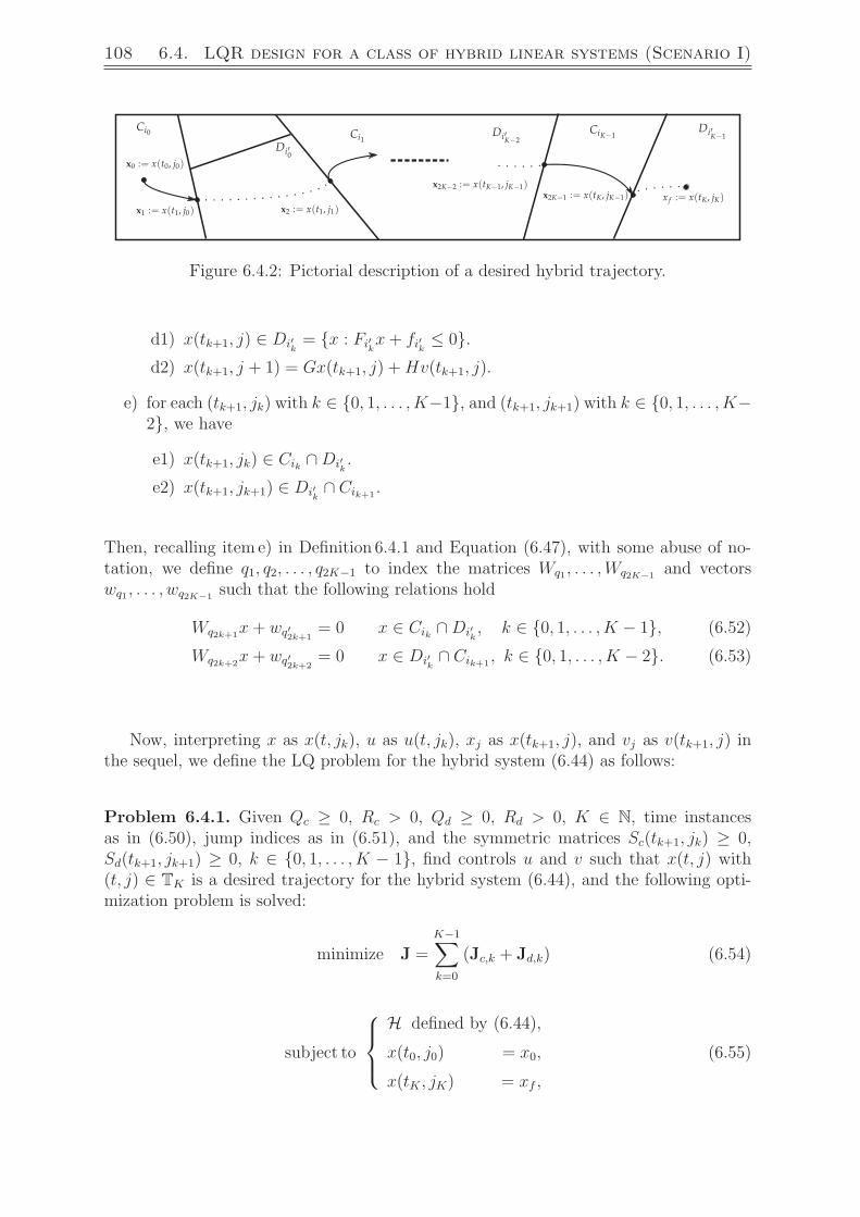
108 6.4. LQR design for a class of hybrid linear systems (Scenario I)
Ci0
Di′0
Ci1CiK−1Di′K−2
Di′K−1
x0 := x(t0, j0)
x1 := x(t1, j0) x2 := x(t1, j1)
x2K−2 := x(tK−1, jK−1)x2K−1 := x(tK, jK−1) x f := x(tK, jK)
Figure 6.4.2: Pictorial description of a desired hybrid trajectory.
d1) x(tk+1, j) ∈ Di′k = x : Fi′kx+ fi′k ≤ 0.d2) x(tk+1, j + 1) = Gx(tk+1, j) +Hv(tk+1, j).
e) for each (tk+1, jk) with k ∈ 0, 1, . . . , K−1, and (tk+1, jk+1) with k ∈ 0, 1, . . . , K−2, we have
e1) x(tk+1, jk) ∈ Cik ∩Di′k .
e2) x(tk+1, jk+1) ∈ Di′k ∩ Cik+1.
Then, recalling item e) in Definition 6.4.1 and Equation (6.47), with some abuse of no-tation, we define q1, q2, . . . , q2K−1 to index the matrices Wq1 , . . . ,Wq2K−1
and vectorswq1 , . . . , wq2K−1
such that the following relations hold
Wq2k+1x+ wq′2k+1
= 0 x ∈ Cik ∩Di′k , k ∈ 0, 1, . . . , K − 1, (6.52)
Wq2k+2x+ wq′2k+2
= 0 x ∈ Di′k ∩ Cik+1, k ∈ 0, 1, . . . , K − 2. (6.53)
Now, interpreting x as x(t, jk), u as u(t, jk), xj as x(tk+1, j), and vj as v(tk+1, j) inthe sequel, we define the LQ problem for the hybrid system (6.44) as follows:
Problem 6.4.1. Given Qc ≥ 0, Rc > 0, Qd ≥ 0, Rd > 0, K ∈ N, time instancesas in (6.50), jump indices as in (6.51), and the symmetric matrices Sc(tk+1, jk) ≥ 0,Sd(tk+1, jk+1) ≥ 0, k ∈ 0, 1, . . . , K − 1, find controls u and v such that x(t, j) with(t, j) ∈ TK is a desired trajectory for the hybrid system (6.44), and the following opti-mization problem is solved:
minimize J =K−1∑k=0
(Jc,k + Jd,k) (6.54)
subject to
⎧⎪⎨⎪⎩
H defined by (6.44),
x(t0, j0) = x0,
x(tK , jK) = xf ,
(6.55)

Chapter 6. Control of hybrid linear systems 109
where
Jc,k =1
2x(tk+1, jk)
> Sc(tk+1, jk) x(tk+1, jk)+
+1
2
∫ tk+1
tk
[x> Qc x+ u> Rcu] dt, (6.56)
Jd,k =1
2x (tk+1, jk+1)> Sd(tk+1, jk+1) x(tk+1, jk+1)+
+1
2
jk+1−1∑j=jk
[x>j Qd xj + v>j Rd vj]. (6.57)
In this problem setting, Jc,k and Jd,k are the cost variables associated to the timeintervals Tc,k and Td,k for k ∈ 0, . . . , K − 1, respectively. The symmetric matricesSc(tk+1, jk) with k ∈ 0, . . . , K − 1, and Sd(tk+1, jk+1) with k ∈ 0, . . . , K − 2 areused to specify the costs on the boundaries of the flow and jump sets, and Sd(tK , jK) isused to specify the cost at the terminal point x(T, J) = xf . Note that Problem 6.4.1incorporates two control objectives: it seeks controls u and v which move the trajectoryfrom the initial condition x0 to the final destination xf with 2K − 1 switching betweenflow and jump dynamics, and additionally minimizes the cost J defined by (6.54).
Due to the state space constraints and hybrid nature of the system (6.44) solvingProblem 6.4.1 is non-trivial. Consequently, we instead determine controls u and v whichprovide suboptimal solutions for the cost (6.54). The approach we follow for findingthese controls, is first to consider the LQR problems associated to each hybrid timeinterval parameterized by their initial and end states. For these problems, we introduceanalytical suboptimal controls by neglecting the inequality constraints arising from thedescription of the polyhedral sets in (6.46). We further show that the closed-loop systemcan be written in affine form with respect to unknown parameters. Later, introducingstatic optimization problems, we compute the parameters and hence derive suboptimalsolutions to Problem 6.4.1.
6.4.1 Suboptimal solutions to flow equations
Consider a piece of a desired trajectory that evolves on the flow set Cik within the intervalTc,k for some k ∈ 0, . . . , K − 1. Recalling the principle of optimality, given the initialand end conditions in Tc,k the control u which solves Problem 6.4.1 must also minimizethe cost Jc,k associated to this time interval. On the other hand, if we assume the initialstate vector x2k := x(tk, jk) and final state vector x2k+1 := x(tk+1, jk) as parameters,then finding the control u which addresses item c) of Definition 6.4.1 as a constraint and

110 6.4. LQR design for a class of hybrid linear systems (Scenario I)
solves the following optimization problem, is motivated by Problem 6.4.1:
minimize Jc,k (6.58)
subject to
x = Ax+Bu,
x(tk, jk) = x2k,
x(tk+1, jk) = x2k+1,
Eikx+ eik ≤ 0.
Here, we formally need the convention x0 = x0 to allow k taking value 0.
Given Sc(tk+1, jk) ≥ 0, Qc ≥ 0, and Rc > 0, a lower bound for this problem canbe given in analytical form by neglecting the inequality constraint in (6.58) and onlyconsidering the fixed initial and end states as the constraints. This solution can bewritten as (see, e.g., Lewis and Syrmos (1995), pp.224)
u = −(Kc −R−1c B>VcP
−1c V >c )x−R−1
c B>VcP−1c x2k+1, (6.59)
where
−Sc = A>Sc + ScA− ScBR−1c B>Sc +Qc,
Kc = R−1c B>Sc,
−Vc = (A−BKc)>Vc,
Pc = V >c BR−1c B>Vc, (6.60)
for (t, jk) ∈ Tc,k, and with the boundary conditions
Vc(tk+1, jk) = I, Pc(tk+1, jk) = 0,
and the given Sc(tk+1, jk); see Appendix A.8.3.
In (6.60), the auxiliary variable Vc ∈ Rn×n is a “modified state transition matrix”for the adjoint of the linear time varying closed loop system, and −Pc(t, jk) ∈ Rn×n isa sort of weighted reachability gramian. If det(Pc(t, jk)) = 0 for all (t, jk) ∈ Tc,k, theproblem is abnormal and no solution exists. For this reason, we assume Pc is non-singularwithin these time intervals. Note that if Qc = 0, non-singularity of Pc is implied bycontrollability of the pair (A,B); see Lewis and Syrmos (1995). Moreover, the variables
θc,k := θc(t, jk) = −Pc(t, jk)−1 [Vc(t, jk)> x− x2k+1]
are constant in the interval Tc,k, and the costate parameters λc(t, jk) are given by
λc(t, jk) = Sc(t, jk) x+ Vc(t, jk) θc,k. (6.61)
Furthermore, referring to (6.59) and (6.61), the relationship between the costate and thecontrol is given by
u = −R−1c B>λc(t, jk).
Chapter 6. Control of hybrid linear systems 111
Note that in (6.60), the first Riccati equation for Sc, as well as the differential equationsfor Vc and Pc, are solved backwards in time up to (tk, jk), within any time interval Tc,k;see Lewis and Syrmos (1995).
Now, a suboptimal value of the cost Jc,k with the state feedback control given by(6.59) can be analytically computed in the following. Note that throughout this chapterthe symbol ∗ denotes an optimal value of a variable and must be distinguished by theconjugate transpose symbol used in the previous chapters.
Lemma 6.4.1. (Kouhi et al., 2013b; Bryson and Ho, 1975)) A lower bound for theoptimal value of the cost Jc,k in Problem (6.58) with the control (6.59) is given by
Jl∗c,k = 1
2x>2k Sc(tk, jk) x2k − 1
2
[Vc(tk, jk)
> x2k − x2k+1
]>× Pc(tk, jk)−1 [Vc(tk, jk)
> x2k − x2k+1]. (6.62)
Proof: Rewrite the control (6.59) in the more convenient form
u = −R−1c B>
(Scx− VcP−1
c z), (6.63)
where for reducing the computation we defined the variable
z(t, jk) = Vc(t, jk)> x− x2k+1.
From the definitions of Kc, Vc, and Pc in (6.60), and the definition of u in (6.59), wehave
z = V >c x+ V >c x
= −V >c (A−BKc) + V >c (Ax+Bu)
= V >c BR−1c B>VcP
−1c [Vc(tk, jk)
> x− x2k+1]
= PcP−1c z.
Consequently, we can obtain the following equality
ddt
[z>P−1
c z]
= 2z>Pcz − z>P−1c PcP
−1c z
= z>P−1c PcP
−1c z. (6.64)
Then, by utilizing (6.60), (6.63) and (6.64), we have
x>Qcx+ u>Rcu =
= x>Qcx+[Sc x− VcP−1
c z]>BR−1
c B>[Sc x− VcP−1
c z]
= x>(−Sc − A>Sc − ScA+ ScBR−1c B>Sc) x
+ x> ScBR−1c B>Sc x− 2x> ScBR
−1c B>VcP
−1c z + z> P−1
c PcP−1c z
=[−x>Sc x− (Ax+Bu)>Sc x− x> Sc(Ax+Bu)
]+ d
dt[z> P−1
c z]
= ddt
[−x> Sc x+ z> P−1c z]. (6.65)

112 6.4. LQR design for a class of hybrid linear systems (Scenario I)
Hence, from the definition of Jc,k in (6.56), the suboptimal cost equals
Jl∗c,k = 12x(tk+1, jk)
> Sc(tk+1, jk) x(tk+1, jk)
− 12[x(t, jk)
> Sc(t, jk) x(t, jk)]tk+1
tk
+ 12
[z(t, jk)
> Pc(t, jk)−1 z(t, jk)
]tk+1
tk
= 12x>2k Sc(tk, jk) x2k − 1
2z(tk, jk)
> Pc(tk, jk)−1 z(tk, jk).
Note that in the last equation we used the fact
z(tk+1, jk)> Pc(tk+1, jk)
−1 z(tk+1, jk) = 0.
Now, with the control (6.59), the resulting closed-loop system turns out to be a lineartime varying system
x = Mc(t, jk) x+Nc(t, jk) x2k+1, (6.66)
with
Mc(t, jk) = A−BR−1c B>
(Sc(t, jk)− Vc(t, jk) Pc(t, jk)−1 Vc(t, jk)
>),
and
Nc(t, jk) = −BR−1c B>Vc(t, jk) Pc(t, jk)
−1.
As a consequence, the solution of (6.66) is affine with respect to x2k and x2k+1; namely
x(t, jk) = Mc(t, tk, jk) x2k + Nc(t, jk) x2k+1, (6.67)
where Mc(t, tk, jk) ∈ Rn×n and Nc(t, jk) ∈ Rn×n are given by
Mc(t, tk, jk) = Mc(t, jk) Mc(t, tk, jk) Mc(τ, τ, jk) = In,
Nc(t, jk) =
∫ t
tk
Mc(t, τ, jk) Nc(τ, jk) dτ ; (6.68)
see Appendix A.5. The function Mc represents the state-transition matrix. The com-putation of Mc(t, tk, jk) can be accomplished by solving the corresponding differentialequation forward in time.
6.4.2 Suboptimal solutions for jumps
Consider a piece of a desired trajectory which evolves on the jump set Di′kand satisfies
item d) in Definition 6.4.1 corresponding to the interval Td,k. Then, the optimal control vwhich solves Problem 6.4.1 must minimize the cost Jd,k in (6.56) associated to this timeinterval. On the other hand, if we consider the initial state vector x2k+1 := x(tk+1, jk)

Chapter 6. Control of hybrid linear systems 113
and final state vector x2k+2 := x(tk+1, jk+1) as parameters, then finding a control v whichminimizes the cost Jd,k in the following problem is required in Problem 6.4.1:
minimize Jd,k
subject to
x+ = Gx+Hv,
x(tk+1, jk) = x2k+1,
x(tk+1, jk+1) = x2k+2,
Fi′kx+ fi′k ≤ 0.
(6.69)
Here, we need the formal convention x2K = xf to allow k taking value K−1. Neglectingthe inequality constraint in (6.69), Problem (6.69) will be again a standard discrete LQRproblem with initial and final states as parameters. Its solution is known and availableanalytically (see Lewis and Syrmos (1995), p.p 250). For simplicity of notation, wedenote
Sd,j = Sd(tk+1, j), Pd,j = Pd(tk+1, j), Vd,j = Vd(tk+1, j).
Then, given Sd(tk+1, jk+1) ≥ 0, Qd ≥ 0, and Rd > 0 the suboptimal control reads
vj = −Kj x+Kvj Vd,j+1 P
−1d,j [V >d,j xj − x2k+2], (6.70)
where
Kj = (H> Sd,j+1 H +Rd)−1 H> Sd,j+1 G,
Sd,j = G> Sd,j+1 (G−HKj) +Qd,
Vd,j = (G−H Kj)>Vd,j+1,
Pd,j = Pd,j+1 − V >d,j+1H (H> Sd,j+1H +Rd)−1 H> Vd,j+1,
Kvj = (H> Sd,j+1 H +Rd)
−1 H>, (6.71)
and the boundary conditions
Pd(tk+1, jk+1) = Pd,jk+1= 0, Vd(tk+1, jk+1) = Vd,jk+1
= I, Sd,jk+1= Sd(tk+1, jk+1),
hold; see Appendix A.8.4. Note that Sd(tk+1, jk+1) according to the assumption ofProblem 6.4.1 is given.
In (6.70), the auxiliary variables Vd,j ∈ Rn×n are the “modified state transition ma-trices” for the adjoint of the time varying closed-loop system, and −Pd,j ∈ Rn×n is asort of weighted reachability gramian; see Lewis and Syrmos (1995). The problem hasa solution if and only if det (Pd(tk+1, jk)) 6= 0. Thus, it is natural to assume that non-singularity of Pd holds within these time intervals. Note that if Qd = 0, controllabilityof (G,H) suffices for non-singularity of Pd; see Lewis and Syrmos (1995). If for somejk < j ≤ jk+1, det (Pd,j) = 0, then the control (6.70) needs to be modified to
vj = −Kj xj +Kvj Vd,j+1 P
−1d,jk
[V >d,jk x2k+1 − x2k+2].

114 6.4. LQR design for a class of hybrid linear systems (Scenario I)
Moreover, in this form of solutions the co-state parameters λd(tk, j) are given in the formof
λd,j = Sd,j xj + Vd,j θd,j, (6.72)
where the variables
θd,k = θd,j := −P−1d,j [V >d,j xj − x2k+2], (6.73)
are constant in each discrete interval Td,k. Furthermore, referring to (6.70) and (6.72),the relationship between the co-state and the control is given by
vj = −R−1d G> λd,j.
Similarly to the continuous evolution, the first Riccati equation for Sd, as well as thedifference equations for Vd and Pd in (6.71) are solved backwards in time up to (tk+1, jk)within any interval Td,k. Now, the suboptimal value of the cost Jd,k with the statefeedback control given by (6.69) can be given in analytical form as follows:
Lemma 6.4.2. (Kouhi et al., 2013b)) A lower bound for the optimal value of the costJd,k in Problem (6.69) with the control (6.70) is given by
Jl∗d,k = 12
x>2k+1 Sd(tk+1, jk) x2k+1 − 12
[Vd(tk+1, jk)> x2k+1 − x2k+2]>×
× Pd(tk+1, jk)−1 [Vd(tk+1, jk)
> x2k+1 − x2k+2]. (6.74)
Proof: Let us define a new variable
zj = V >d,j xj − x2k+2.
Then, recalling the equations for Vd,j from (6.71) and vj in (6.70), we can deduce
zj − zj+1 = V >d,j xj − V >d,j+1 xj+1
= V >d,j+1 (G−HKj) xj − V >d,j+1(Gxj +Hvj)
= −V >d,j+1 H Kvj Vd,j+1 P
−1d,j zj.
Therefore, using the difference equation for Pd,j and the equation of Kvj from (6.71), we
can compute zj+1 as
zj+1 = (Pd,j + V >d,j+1 HKvj Vd,j+1) P−1
d,j zj
= Pd,j+1 P−1d,j zj.
It follows that
z>j P−1d,j (Pd,j − Pd,j+1) P−1
d,j zj =
= z>j P−1d,j zj − z>j+1 P
−1d,j+1 zj+1. (6.75)
Chapter 6. Control of hybrid linear systems 115
Furthermore, from (6.71) we have
x>j+1 Sd,j+1 xj+1 =
= (Gxj +Hvj)> Sd,j+1 (Gxj +Hvj)
= x>j G> Sd,j+1 G xj + 2x>j G> Sd,j+1 H vj
− v>j Rd vj + v>j (H> Sd,j+1 H +Rd) vj. (6.76)
Then, from the last equation we can compute
v>j Rd vj = −x>j+1 Sd,j+1 xj+1 + x>j G> Sd,j+1 G xj
+ 2x>j G> Sd,j+1H vj + v>j (H> Sd,j+1 H +Rd)vj. (6.77)
To prove (6.74), we now exploit (6.70), (6.71), (6.75), and (6.77) for the evaluation ofthe summing terms in the cost variable. To this end, introduce a new variable
yj = x>j Sd,j xj − x>j+1 Sd,j+1 xj+1
to simplify the computations. Then, we have
x>j Qd xj + v>j Rd vj =
= x>j
[Sd,j −G>Sd,j+1 (G−H Kj)
]xj − x>j+1 Sd,j+1 xj+1
+ x>j G> Sd,j+1 G xj + 2x>j G> Sd,j+1 H vj + v>j (H S>d,j+1 H +Rd) vj
= yj + x>j G> Sd,j+1 H (Kj xj + vj)︸ ︷︷ ︸Kvj Vd,j+1 P−1
d,j zj
+ [v>j + x>j G>Sd,j+1 H (H> Sd,j+1 H +Rd)−1︸ ︷︷ ︸
K>j
] (H> Sd,j+1 H +Rd) vj
= yj + [x>j G> Sd,j+1 H + v>j (H> Sd,j+1 H +Rd)︸ ︷︷ ︸z>j P−1
d,j V >d,j+1 Kv>j (H> Sd,j+1 H+Rd)
] Kvj Vd,j+1 P
−1d,j zj
= yj + z>j P−1d,j V
>d,j+1H(H>Sd,j+1H +Rd)
−1H>Vd,j+1︸ ︷︷ ︸Pd,j+1−Pd,j
P−1d,j zj
= yj − z>j P−1d,j zj + z>j+1 P
−1d,j+1 zj+1.
Now summing up the terms resulted from the previous equation with the terminal costof this time interval, Jd,k defined by (6.57) equals
Jd,k = 12x (tk+1, jk+1)> Sd(tk+1, jk+1) x(tk+1, jk+1)+
+ 12
jk+1−1∑j=jk
[x>j Qd xj + v>j Rd vj]
= 12x (tk+1, jk+1)> Sd(tk+1, jk+1) x(tk+1, jk+1)
+ 12
jk+1−1∑j=jk
[yj − z>j P−1d,j zj + z>j+1 P
−1d,j+1 zj+1]
= 12
x>2k+1 Sd(tk+1, jk) x2k+1
− 12z(tk+1, jk)
> Pd(tk+1, jk)−1 z(tk+1, jk),

116 6.4. LQR design for a class of hybrid linear systems (Scenario I)
where we used the identity
z(tk+1, jk+1)> Pd(tk+1, jk+1)−1 z(tk+1, jk+1) = 0.
Note that the closed-loop system with the affine control defined in (6.70) is againdescribed by a linear time varying difference equation:
xj+1 = Md(tk+1, j) xj +Nd(tk+1, j) x2k+2, (6.78)
with the coefficients
Md(tk+1, j) = G−H Kvj (Sd,j+1 G− Vd,j+1 P
−1d,j V
>d,j),
and
Nd(tk+1, j) = −H Kvj Vd,j+1 P
−1d,j .
The solution to (6.78) is an affine function in x2k+1 and x2k+2, that is,
xj = Md(tk+1, j) x2k+1 + Nd(tk+1, j) x2k+2, (6.79)
where the coefficients are given by
Md(tk+1, j) =
j−jk∏r=0
Md(tk+1, j − r), Md(tk+1, jk) = In,
Nd(tk+1, j) =
j−1∑r=jk
j−r−1∏p=1
Md(tk+1, j − p) Nd(tk+1, r),
and Nd(tk+1, jk) = 0. This fact will be utilized in the next section for imposing theinequality constraints for deriving a desired trajectory.
6.4.3 Constrained QP problems for the hybrid linear system
Having discussed the analytical suboptimal solutions to the optimal control problemsseparately for the flow and jump dynamics, in this section we consider them jointlyfor establishing a link to Problem 6.4.1. From the elaborations in the previous twosubsections, we know that neglecting the inequality constraints of the polyhedral sets,the suboptimal cost in each hybrid time interval can be parametrized quadraticallyby parameters x2k and x2k+1 given by (6.62), or x2k+1 and x2k+2 given by (6.74) fork ∈ 0, 1, . . . , K − 1. Hence, the overall suboptimal cost equals
J =K−1∑k=0
(Jl∗c,k + Jl∗d,k
)=
1
2X>PX +QX +R, (6.80)
Chapter 6. Control of hybrid linear systems 117
whereX := [x>1 x>2 . . . x>2K−1]>,
includes all unknown parameters, and P = [Pij] ∈ R(2K−1)n×(2K−1)n is a symmetricmatrix of the form
P =
P11 P12 0 . . . 0P21 P22 P23 . . . 0
0 P32. . . . . .
......
.... . . P2K−2,2K−2 P2K−2,2K−1
0 0 . . . P2K−1,2K−2 P2K−1,2K−1
with the symmetric matrix elements
Pkk =
−Pc(tk−1, jk−1)−1 + Sd(tk, jk−1)− Vd(tk, jk−1)Pd(tk, jk−1)−1 Vd(tk, jk−1)>, k odd,
−Pd(tk, jk−1)−1 + Sc(tk, jk)− Vc(tk, jk)Pc(tk, jk)−1 Vc(tk, jk)>, k even,
and
Pk,k+1 = P>k+1,k =
Vd(tk, jk−1) Pd(tk, jk−1)−1, k odd
Vc(tk, jk) Pc(tk, jk)−1, k even.
The element QX +R in the cost (6.80) appears when k = 0 and k = K are considered.The row vector Q ∈ R1×[(2K−1)n] is given by
Q = [x>0 Vc(t0, j0)Pc(t0, j0)−1 0 · · · 0 x>f Vd(tK , jK−1)Pd(tK , jK−1)−1],
and R is a scalar which is given by
R = 12x>0 Sc(t0, j0) x0 − 1
2x>0 Vc(t0, j0) Pc(t0, j0)−1
× Vc(t0, j0)> x0 − 12x>f Pd(tK , jK−1)−1 xf .
Now, the cost defined in (6.80) is parameterized only by the decision variable X. Notethat since Jl∗c,k+Jl∗d,k > 0 for each k ∈ 1, . . . , K−1, we have that 1
2X>PX+QX+R > 0.
In particular, when x0 = 0 and xf = 0, we have that 12X>PX > 0 for all X 6= 0. This
implies that P > 0.
6.4.3.1 Lower bound for optimal control problem
Now, we intend to determine the unknown parameters x1, . . . ,x2K−1 in a way that weobtain a lower bound for the optimal cost of Problem 6.4.1. To this end, we consider theEquations (6.52) and (6.53) as constraints for the minimization of the cost (6.80). Thus,we define a static optimization problem as follows:
minimize J = 12X>PX +QX +R
subject to CX + R = 0, (6.81)

118 6.4. LQR design for a class of hybrid linear systems (Scenario I)
where matrix C and vector R are given by
C = diag([Wq1 ,Wq2 , . . . ,Wq2K−1
]),
R =[w>q1 w>q2 . . . w>q2K−1
]>. (6.82)
The Lagrangian for Problem (6.81) then reads
L(X,λ) = 12X>PX +QX +R + λ>(CX + R),
where λ is the Lagrange multiplier. As P > 0, Problem (6.81) has always a minimum.For finding this optimal value, we assign ∂L/∂X = 0 and use equality constraint in(6.81) to compute an analytical solution for X, denoted by X∗l , as follows:
X∗l = −P−1[Q> −C>(CP−1C>)−1(CP−1Q> −R)
]. (6.83)
Hence, the optimal value of J in Problem (6.81), denoted by J∗l , is given by
J∗l = 12
[Q+ (QP−1C> −R>)(CP−1C>)−1C
]P−1
×[−Q> + C>(CP−1C>)−1(CP−1Q> −R)
]+R. (6.84)
Note that J∗l is indeed the optimal cost for Problem 6.4.1 when the inequality constraintsgiven in Problems (6.58) and (6.69) for k = 0, . . . , K − 1, which capture the flow andjump sets, are neglected. Therefore, we have J∗l ≤ J∗.
6.4.3.2 Algorithm to compute solution and an upper bound
Now, we aim at determining the controls u and v, such that the solution of the hybridsystem (6.44) becomes a desired trajectory, and an upper bound for the cost J∗ definedin Problem 6.4.1 is derived. To this end, we consider the inequality constraints given inProblems (6.58) and (6.69) for minimization of the cost (6.80) in order to ensure that allcriteria (a-f) in Definition 6.4.1 hold. Notice (6.67) and (6.79) indicate that each pointof the suboptimal trajectory has the affine representation with respect to the decisionvariables x1, . . . ,x2K−1. Now, we insert x(t, jk) from (6.67) into the inequality constraints(6.58),
Eik x(t, jk) + eik ≤ 0 (6.85)
for all time (t, jk) ∈ Tc,k, and insert x(tk+1, j) from (6.79) into the inequality constraintgiven in (6.69), namely
Fi′k x(tk+1, j) + fi′k ≤ 0, (6.86)
for all (tk+1, j) ∈ Td,k. Thus, for each k ∈ 0, . . . , K − 1, (6.85) and (6.86) can beexpressed in the matrix form as
Xc(t, j)X + Yc(t, j) ≤ 0, (6.87)

Chapter 6. Control of hybrid linear systems 119
and
Xd(t, j)X + Yd(t, j) ≤ 0, (6.88)
where
Xc(t, j) =
[Ei0Nc(t, j0) 0 . . . 0] ∀(t, j) ∈ Tc,0,
[0 . . . EikMc(t, tk, jk) EikNc(t, jk) . . . 0] ∀(t, j) ∈ Tc,k, k ≥ 1,
Yc(t, j) =
[x>0 Mc(t, t0, j0)>E>i0 + e>i0 0 . . . 0]> ∀(t, j) ∈ Tc,0,
[0 . . . e>ik . . . 0]> ∀(t, j) ∈ Tc,k, k ≥ 1,
Xd(t, j) =
[0 . . . Fi′kMd(tk, j) Fi′kNd(tk, j) 0 . . . 0] ∀(t, j) ∈ Td,k, k ≤ K − 2,
[0 . . . 0 Fi′K−1Md(tK , j)] ∀(t, j) ∈ Td,K−1,
and
Yd(t, j) =
[0 . . . f>i′k
. . . 0]> ∀(t, j) ∈ Td,k, k ≤ K − 2,
[0 . . . 0 x>f Nd(tK , j)>F>i′K−1
+ f>i′K−1]> ∀(t, j) ∈ Td,K−1.
Now, considering the inequality constraints (6.87) and (6.88) for minimization of the cost(6.80), and for k ∈ 0, . . . , K − 1 we define the following static optimization problem:
minimize J = 12X>PX +QX +R (6.89)
subject to
Xc(t, j)X + Yc(t, j) ≤ 0 ∀(t, j) ∈ Tc,k,
Xd(t, j)X + Yd(t, j)≤ 0 ∀(t, j) ∈ Td,k.
Problem (6.89) consists of a quadratic cost and a set of infinitely many affine inequalitiesdue to the continuity of time. However, note that the matrices Xc(t, j) and the vectorsYc(t, j) implicitly depend on the variables Sc, Pc, and Vc which are computed numericallyvia solving the ODE in (6.60) with certain sample times. Therefore, the number ofinequalities in (6.89) is finite from a numerical point of view. Suppose the number ofthe time samples are N ∈ N. Therefore, (6.89) can be rewritten as
minimize J = 12X>PX +QX +R (6.90)
subject to
Xc X + Yc ≤ 0,Xd X + Yd ≤ 0,

120 6.4. LQR design for a class of hybrid linear systems (Scenario I)
where the matrix Xc ∈ RN×(2K−1)n and the vector Yc ∈ RN , the matrix Xd ∈ RJ×(2K−1)n
and the vector Yd ∈ RJ are defined by
Xc =
Xc(0, 0)...
Xc(T, jK−1)
, Yc =
Yc(0, 0)...
Yc(T, jK−1)
,
Xd =
Xd(0, 0)...
Xd(T, J)
, Yd =
Yd(0, 0)...
Yd(T, J)
.Problem (6.90) consists of a quadratic cost and a finite set of inequalities defining
a standard quadratic program (QP). It is well known that if P is positive definite,then the entire problem is convex and can be solved in polynomial time; otherwise, theproblem is NP hard. Quadratic problems are well understood and plenty of establishednumerical and analytical algorithms are available, including interior point methods,active set, etc; see Nocedal and Wright (2006); Bayon et al. (2010).
Next we want to provide a numerical algorithm for solving Problem (6.90) by employ-ing the dual optimal control theory and gradient projection method (see, e.g., Boyd andVandenberghe (2004)), provided that the problem is feasible. To this end, the Lagrangianof the cost reads
L(X,λc, λd) = 12X>PX +QX +R+
+ λ>c (XcX + Yc) + λ>d (XdX + Yd),
whereλc ≥ 0, λd ≥ 0,
are Lagrange multipliers. Then, the dual problem of (6.90) is given by
maximize g(λc, λd),
subject to λc, λd ≥ 0, (6.91)
where the function g is defined by
g(λc, λd) = infXL(X,λc, λd).
Since all inequalities in (6.90) are affine with respect to X and P > 0, strong dualityis given by the Slater condition (Boyd and Vandenberghe, 2004), implying that optimalsolutions to the dual and primal problems are identical. Starting from an arbitrary initialcondition λ
(0)c and λ
(0)d , the solution to the dual problem is determined by an iterative
algorithm for computation of the Lagrange multipliers
λ(r+1)c = λ(r)
c − α(Xc X(r)u + Yc),
λ(r+1)d = λ
(r)d − α(Xd X
(r)u + Yd). (6.92)
Chapter 6. Control of hybrid linear systems 121
where 0 < α < 1 represents a fixed step size, r represents the rth update of the variables,and the index u in Xu refers to the upper bound control algorithm. After each iteration,the Lagrange multipliers λ
(r)c and λ
(r)d are projected in accordance with
[λ(r+1)c , λ
(r+1)d ] = [max(0, λ(r+1)
c ), max(0, λ(r+1)d )]. (6.93)
The variable X(r)u in the last equation can be analytically computed in terms of the
Lagrange multipliers by differentiating the Lagrangian L(X(r)u , λ
(r)c , λ
(r)d ) with respect to
X(r)u and setting it to zero, that is,
X>c λ(r)c + X>d λ
(r)d +Q> + P X(r)
u = 0
⇒ X(r)u = −P−1(X>c λ(r)
c + X>d λ(r)d +Q>). (6.94)
Now, let us define
Λ(r) := [ λ(r)>
c λ(r)>
d ]>.
Then, replacing (6.94) into (6.92), the update law for the gradient projection methodreads (see Boyd and Vandenberghe (2004)):
Λ(r+1) =
I + αXcP−1X>c αXcP
−1X>dαXdP
−1X>c I + αXdP−1X>d
Λ(r) − α
Yc − XcP−1Q>
Yd − XdP−1Q>
. (6.95)
Equation (6.93) contains a nonlinear operation, thus we are not able to compute Λ(r)
analytically. However, we can describe the equation (6.94) in the matrix form as
X(r)u = −P−1
(Q> + X Λ(r)
), (6.96)
where X := [X>c X>d ]. It follows from the gradient projection method that
limr→∞
X(r)u → X∗u, and lim
r→∞Λ(r) → Λ∗.
Therefore, the optimal cost results to be:
J∗u =1
2(−Q> + XΛ∗)>P−1(Q> + XΛ∗) +R. (6.97)
The cost J∗u indeed provides an upper bound for the optimal cost J∗ in Problem 6.4.1.The reason is that the trajectory which uses the solutions of Problem (6.90) with controlsu, defined by (6.59), and v, defined by (6.70), satisfies all conditions of Definition 6.4.1.Nevertheless, the equality J∗u = J∗ does not necessarily hold since the controls u and vin (6.59) and (6.70) are computed via neglecting the inequalities given on (6.58) and(6.69). Thus, this trajectory is not necessarily optimal in the sense of Problem 6.4.1.
The following theorem summarizes this result.

122 6.4. LQR design for a class of hybrid linear systems (Scenario I)
Theorem 6.4.1. Consider the linear quadratic problem for the hybrid linear system(6.44) defined by Problem 6.4.1. Suppose that the optimization problem (6.90) is feasible.Then, the optimal cost J∗ defined in Problem 6.4.1 is bounded by
J∗l ≤ J∗ ≤ J∗u, (6.98)
with J∗l and J∗u given by expressions (6.84) and (6.97), respectively.
Example 6.4.1. (See also (Kouhi et al., 2013b)) Consider the hybrid linear system
H :
x =
[−1 1
2 −3
]x+
[1 12 1
]u x ∈ C,
x+ =
[0.7 0.50 0.8
]x+
[0.125 0.50.5 0.2
]v x ∈ D,
where denoting x = [x1 x2]>, the sets C and D are specified by
C = x ∈ R2 : 2x1 − x2 ≤ 0, D = R2\C.
The corresponding cost variables are defined by
Jc,k = 12
∫ tk+1
tk
(x>[
2 00 2
]x+ u>
[1 00 1
]u
)dt,
Jd,k =1
2
jk+1−1∑j=jk
x>j
[2 11 1
]xj + v>j
[1 00 1
]vj,
where K = 2 is a fixed parameter, indicating that only three switching between the flowand jump sets must occur. Then, the overall cost J is defined by (6.54). The switchingtime instances are fixed and given by
(t1, j0) = (0.2, 0), (t1, j1) = (0.2, 4), and (t2, j1) = (1, 4),
and the fixed final time equals (t2, j2) := (T, J) = (1, 8). Thus, the time domain equals
TK =([0, 0.2]× 0) ∪ (0.2 × 0, . . . , 4)∪ ([0.2, 1]× 4) ∪ (1 × 4, . . . , 8).
The fixed initial and final states are given by x0 = [3 7]> ∈ C and xf = [3 − 1]> ∈ D,respectively. The cost associated to the switching points and to the terminal point arezero. Two trajectories computed via our algorithm are depicted in Figure 6.4.3. Theflow evolution is represented by the curves with solid lines, and the jump evolution bysmall circles. The top picture refers to the solution obtained by lower bound control forthe hybrid system with neglected inequality constraints arising from the definition of theflow and jump sets. One can observe that inequality constraints in definition of the flow

Chapter 6. Control of hybrid linear systems 123
−2 −1 0 1 2 3 4 5 6
−2
0
2
4
6
8
0 1 2 3 4 5 6
0
2
4
6
8
x1
x 2
x1
x 2
x0
x0
x f
x f
D
D
C
C
Figure 6.4.3: (Top:) The trajectory resulting from the control policy achieves theprovided lower bound of the cost by ignoring the inequality constraints. (Bottom:) Thesystem trajectory resulting from the control policy achieves the provided upper boundof the cost.
and jump sets are violated. Note that this trajectory principally does not belong to thesolution set of this system since a trajectory of the hybrid system cannot jump within theset C. In contrary, in the bottom picture the solution resulting from the upper boundcontrol is a desired trajectory of the hybrid system. The parameters x1, x2, and x3 inthe lower bound optimal control problem defined in Section 6.4.3.1 are computed to be
x1 = [−0.9512 − 1.9024], x2 = [0.60 1.20], x3 = [0.60 1.20],
incidentally, with two latter variables being identical. The parameters for the upperbound control problem defined in Section 6.4.3.2 are computed to be
x1 = [1.0820 2.1640], x2 = [0.0446 0.0893], x3 = [0.0095 0.0189].
For this problem the following upper and lower bounds for the optimal cost J∗ arecomputed as
585.3010 ≤ J∗ ≤ 658.3335.
124 6.5. LQR design for a class of hybrid linear systems (Scenario II)
6.5 LQR design for a class of hybrid linear systems
(Scenario II)
In this section, we address a problem that relates maximum principle (Sussmann, 1999;Caines et al., 2006; Johansen et al., 2002; Liberzon, 2011) to a class of hybrid linearsystems.
Let us consider a hybrid linear system H consisting of different linear flow dynamicsgiven by
H :
x = Aσ(t,x)x+Bσ(t,x)u x ∈ C,x+ = x x ∈ D,
(6.99)
where σ(t, x) ∈ L := 1, . . . , ` is the switching signal between different dynamics. Weassume that switching to a new dynamics can only occur when the states of the systembelong to the jump set. Suppose also
Aσ(t,x) ∈ A ∈ A1, . . . , A`, Bσ(t,x) ∈ B := B1, . . . , B`, (6.100)
where u(t) ∈ Rm, Ai ∈ Rn×n, Bi ∈ Rn×m, and the pairs (Ai, Bi) are controllable for alli ∈ L. Further, we assume C = Rn and
D = ∪i∈I Di, (6.101)
where the jump set D is the union of switching manifolds given by the affine equationsin the state space as
Di = x ∈ Rn : cix+ ri = 0 ∀i ∈ I. (6.102)
In (6.102), I is a finite index set, ci are matrices, and ri are vectors with appropriatedimensions, for all i ∈ I. Given K ∈ N and T ∈ R>0, assume the switching time instancest1, . . . , tK−1 between different dynamics exist such that
0 := t0 < t1 . . . < tK−1 < tK =: T. (6.103)
For this system, we define the hybrid time domain as follows:
TK :=K−1⋃k=0
Tk,
where
Tk = [tk, tk+1]× k ∀k ∈ 0, . . . , K − 1. (6.104)
Note that with these assumptions and the definition of the hybrid system in (6.99), themapping (t, k) 7→ x(t, k) is absolutely continuous over the hybrid time domain. For adefinition of absolute continuity see Appendix A.6.1. Interpreting x as x(t, k), we definean LQ problem for the hybrid system (6.99) as follows:

Chapter 6. Control of hybrid linear systems 125
Problem 6.5.1. Given a number K ∈ N, matrices Qk ≥ 0 and Rk > 0 for eachk ∈ 0, . . . , K − 1, symmetric matrices Sc(tk+1, k) ≥ 0 for each k ∈ 0, 1, . . . , K − 1,and a sequence of switching, that is, Aσ(t,x) = Ajk ∈ A and Bσ(t,x) = Bjk ∈ B for all(t, k) ∈ TK are fixed. Moreover, assume that the final time tK = T is given and either:
a) the time instances t1, . . . , tK−1 satisfying (6.103) are given.
b) the time instances t1, . . . , tK−1 satisfying (6.103) are unknown.
Find the control u (and the switching time instances for case b)), such that the followingoptimization problem is solved:
minimize J =K−1∑k=0
Jk (6.105)
subject to
H defined by (6.99),
x(t0, 0) ∈ Di0 i0 ∈ I,
x(tk+1, k) ∈ Dik+1∀k ∈ 0, . . . , K − 1, ik ∈ I,
(6.106)
where
Jk =1
2x(tk+1, k)>S(tk+1, k)x(tk+1, k) +
1
2
∫ tk+1
tk
[x> Qk x+ u> Rk u] dt, (6.107)
for all k ∈ 0, . . . , K − 1.
In (6.107) the given symmetric matrices S(tk+1, k) for each k ∈ 0, 1, . . . , K − 2 areused to specify the cost variables corresponding to the switching time instances, andS(tK , K−1) is used to specify the cost variable at an end point x(T,K−1) = xf ∈ DiK .Problem 6.5.1 is fairly general and we can solve the following scenarios by finding asolution to this problem.
i) The switching times with regard to case a) in Problem 6.5.1 are fixed. We call thisproblem “fixed switching times problem”.
ii) The switching times are free as represented by case b) of Problem 6.5.1. We referto this problem as “free switching times problem”.
iii) The initial state vector x0 and the terminal state vector xf are fixed. This conditionis equivalent to have
ci0 = I, ri0 = x0, ciK = I, riK = xf .
iv) Item iii), and the conditions Dik = Rn for all k ∈ 1, . . . , K − 1 and ik ∈ Ihold. Then, σ(t, x) = σ(t) and Problem 6.5.1 is reduced to computation ofan optimal control u and switching time instances t1, . . . , tK−1, which minimizethe cost (6.105). In this case, a switching can occur at each point of the state space.

126 6.5. LQR design for a class of hybrid linear systems (Scenario II)
Our solution approach is based on parameterization of the optimal control problemwith respect to initial and end points of each switching time interval, similar to theapproach for solving Problem 6.4.1. To this end, first we represent the LQR problem fora piece of trajectory and parameterize the problem by the initial and end points of eachswitching time interval. We derive an analytical expression for the optimal cost usingthe sweeping method presented by Lewis and Syrmos (1995). This allows us to find ananalytical expression for the entire cost J. Afterwards, we determine the switching timesand states in the next step.
6.5.1 Optimal solution for a piece of a trajectory
Consider a piece of hybrid trajectory that evolves with the dynamics as described by(6.99) within a time interval (t, k) ∈ Tk for some k ∈ 0, . . . , K − 1. Referring tothe principle of optimality, if Problem 6.5.1 has an optimal solution, then each piece ofthe optimal trajectory between two consecutive switching points xk and xk+1 must beoptimal. In other words, if we assume the initial state vector xk := x(tk, k) and the finalstate vector xk+1 := x(tk+1, k) are parameters, then solving the following optimizationproblem for a trajectory x(t, k) that satisfies the differential equation (6.99) for σ(t, x) =jk ∈ L, is motivated by Problem 6.5.1:
minimize Jk
subject to
x = Ajk x+Bjk u,
x(tk, k) = xk,
x(tk+1, k) = xk+1.
(6.108)
Now, Problem (6.108) represents an optimal control problem with initial and endpoints as parameters. The solution is given by (see Lewis and Syrmos (1995), pp.224)
u = −R−1k B>jk
(Sx− V P−1 [V > x− xk+1]
), (6.109)
where
−S = A>jk S + S Ajk − S Bjk R−1k B>jk S +Qk,
Kk = R−1k B>jk S,
−V = (Ajk −Bjk Kk)> V,
P = V > Bjk R−1k B>jkV, (6.110)
for each (t, k) ∈ Tk and with the boundary conditions
V (tk+1, k) = I, P (tk+1, k) = 0, and given S(tk+1, k) ≥ 0.
In the solution (6.110), the auxiliary variable V (t, k) ∈ Rn×n is a “modified statetransition matrix” for the adjoint of the linear time varying closed loop system, and−P (t, j) ∈ Rn×n is a sort of weighted reachability gramian. If det(P (t, k)) = 0 for all
Chapter 6. Control of hybrid linear systems 127
(t, k) ∈ Tk, the problem is abnormal and no solution exists; see Lewis and Syrmos (1995).However, if Qk = 0 for all k ∈ 0, . . . , K − 1, controllability of the pairs (Ajk , Bjk) issufficient for the existence of solutions. Moreover, in this form of the solutions theco-state parameters λ(t, k) are given in the form of
λ(t, k) = S(t, k) x− V (t, k) P (t, k)−1[V (t, k)> x(t, k)− xk+1
], (6.111)
where the elements
θk := θ(t, k) = −P (t, k)−1 [V (t, k)> x(t, k)− xk+1], (6.112)
are constant in the interval (t, k) ∈ Tk. Furthermore, referring to (6.109) and (6.111),the relationship between the co-state and the control is given by
u(t, k) = −R−1k B>jk λ(t, k) ∀(t, k) ∈ Tk;
see Lewis and Syrmos (1995). Note that in (6.110), the first Riccati equation for S, aswell as the differential equations for V and P , are solved backwards in time within anytime interval.
Now, for simplification of notation, in the sequel, we signify the values of the functionsS, V , and P at the specific time instance (tk, k) by the index k. For example, Sk shouldbe interpreted as S(tk, k). As stated by Lemma 6.4.1 the optimal value of the cost Jkwith the state-feedback given by (6.109) can be represented in analytical form as follows:
J∗k = 12x>k Sk xk − 1
2
[V >k xk − xk+1
]>P−1k [V >k xk − xk+1]. (6.113)
6.5.2 A QP problem for finding the switching points
Having discussed the analytical solutions to optimal control for each piece of the trajec-tory, in this section we consider all of them together. Hence, by (6.113) the overall costequals
J =K−1∑k=0
J∗k =1
2X>MX, (6.114)
where X := [x>0 x>1 . . . x>K ]> includes an initial point x0 = x(t0, 0) ∈ Di0 , switchingpoints x1, . . . ,xK−1, and a terminal point xK = x(tK , K − 1) ∈ DiK . M = [Mij] ∈R[n(K+1)]×[n(K+1)] is a symmetric matrix of the form:
M =
M0,0 M0,1 0 . . . 0M1,0 M11 M12 . . . 0
0 M21. . . . . .
......
.... . . MK−1,K−1 MK−1,K
0 0 . . . MK,K−1 MK,K
,

128 6.5. LQR design for a class of hybrid linear systems (Scenario II)
with the matrix elements
M0,0 = M>0,0 = S0 − V0 P
−10 V >0
Mjj = M>jj = Sj − VjP−1
j V >j − P−1j−1 ∀j ∈ 1, . . . , K − 1,
MKK = M>KK = −P−1
K−1,
Mj,j+1 = M>j+1,j = VjP
−1j ∀j ∈ 0, . . . , K − 1.
Note that the cost defined in (6.114) is parameterized by the decision variable X. Now,we add the required constraints to the optimal cost J to ensure that xk ∈ Dik for eachk ∈ 0, . . . , K. This defines a static optimization problem as
minimize J =1
2X>MX
subject to CX + R = 0, (6.115)
where the matrix C and the vector R include the parameters characterizing the equationsof the jump sets Dik for ik ∈ 0, . . . , K, namely
C = blockdiag([ci0 , . . . , ciK ]), R = [r>i0 . . . r>iK ]>. (6.116)
Now, the cost defined in (6.115) is parameterized only by the decision variable X. Notethat since Jk > 0 for each k ∈ 0, . . . , K − 1, we have that 1
2X>MX > 0. This implies
that M > 0 and Problem (6.115) is convex.
Now, introducing the Lagrange multipliers in the form of Λ =blockdiag ([Λ0, . . . , ΛK ]), the Lagrangian of the cost (6.115) reads
L(X,Λ) = 12X>MX + Λ>(CX + R). (6.117)
6.5.3 Computing optimal switching points
Now, if we set the derivative of the Lagrangian (6.117) with respect to X to zero, then theoptimal switching points can be computed. Consequently, as M > 0, Problem (6.115)has a globally optimal value X given by
X∗ = −M−1C>(CM−1C>)−1R := G(S,V,P), (6.118)
where G is a function of S := (S0, . . . , SK−1), V := (V0, . . . , VK−1), and P :=(P0, . . . , PK−1). Hence, the optimal cost equals
J∗ =1
2R>(CM−1C>)−1R. (6.119)
Note that the matrix M is a function of switching times t1, . . . , tK−1. Thus, for theproblem of fixed switching times which is specified by case a) in Problem 6.5.1, M isgiven. However, for the problem of free switching times M is not known so far, and hasto be determined in the following.

Chapter 6. Control of hybrid linear systems 129
6.5.3.1 Transversality condition and solutions of fixed switching timesproblem
Now, we show that our optimal solution u, given by (6.109), satisfies the so called“transversality conditions”(see Sussmann (1999); Caines et al. (2006); Liberzon (2011))for the points belonging to the jump sets. To this end, recalling (6.113) the Lagrangianof Problem (6.115) can be reformulated as
L(X,Λ) =1
2X>MX + Λ>(CX + R) =
= 12
K−1∑j=0
x>k Skxk−[V >k xk−xk+1
]>P−1k [V >k xk − xk+1] +Λ>k (cikxk+rik)
+Λ>K(ciKxK+riK).
Recall that the optimal value of X in Section 6.5.3 was computed by differentiating theLagrangian with respect to xk and setting it to zero. For an initial condition, this isequivalent to have
∂L(X,Λ)
∂x0
= 0⇒(S0 x0 − V0 P
−10 [V >0 x0 − x1]
)+ c>i0 Λ0 = 0. (6.120)
Likewise, for a point belonging to the jump set Dik , we should have
∂L(X,Λ)
∂xk= 0⇒
(Sk xk − Vk P−1
k [V >k xk − xk+1])
+
+(P−1k−1 [V >k−1 xk−1 − xk]
)+ c>k Λk = 0 ∀k ∈ 1, . . . , K − 1, (6.121)
and finally for a terminal point
∂L(X,Λ)
∂xK= 0⇒
(P−1K−1 [V >K−1 xK−1 − xK ]
)+ c>iK ΛK = 0. (6.122)
As discussed previously, the co-states are defined by (6.111) and the variables θ(t, k) in(6.112) are constant in the time interval Tk for all k ≤ K − 1. Therefore, the co-statescan be rewritten in the form of
λ(tk, k) = Sk xk − Vk P−1k [V >k xk − xk+1], ∀k ∈ 0, . . . , K−1,
λ(tk, k − 1) = S(tk, k − 1) xk − P−1k−1 [V >k−1 xk−1 − xk], ∀k ∈ 1, . . . , K. (6.123)
Thus, (6.121) and (6.123) reveal that
λ(t0, 0) + c>i0 Λ0 = 0, (6.124)
λ(tk, k)− λ(tk, k − 1) + S(tk, k − 1) xk + c>ik Λk = 0, (6.125)
− λ(tK , K − 1) + S(tK , K − 1) + c>iK ΛK = 0. (6.126)
In the literature, conditions (6.124-6.126) are referred to as transversality conditionson the initial point, switching points (jump points), and terminal point, respectively(Sussmann, 1999; Liberzon, 2011). Now, we can present a theorem concerning the fixedswitching times problem.

130 6.5. LQR design for a class of hybrid linear systems (Scenario II)
Theorem 6.5.1. The control (6.109), computed by the ordinary differential equations(6.110), and switching parameters, computed by (6.118), solve the case of the fixedswitching times in Problem 6.5.1. Moreover, the optimal cost (6.105) is equal to(6.119).
Now, solving the free switching times case of Problem 6.5.1 entails deriving the ap-propriate switching time instances t1, . . . , tK−1. This will be presented in the sequel.
6.5.4 Computation of optimal switching time instances
For computing the optimal switching times, we set the partial derivative of the costfunction in (6.115) with respect to the switching time tk to zero. In other words,
∂J∗
∂tk= 0⇒ ∂J∗k−1
∂tk+∂J∗k∂tk
= 0 ∀k ∈ 1, . . . , K − 1. (6.127)
Now, we aim at showing that the following relations hold
∂J∗k∂tk
= −H(λ,xk, (tk, k)
)= −
[1
2
(x>kQkxk + u(tk, k)> Rk u(tk, k)
)+
λ(tk, k)> (Ajk xk +Bjk u(tk, k))],
∂J∗k−1
∂tk= H
(λ,xk, (tk, k − 1)
)=
1
2
(x>k Qk−1 xk + u(tk, k − 1)> Rk−1 u(tk, k − 1)
)+ λ(tk, k − 1)>
(Ajk−1
xk +Bjk−1u(tk, k − 1)
). (6.128)
Note that (6.128) in fact represents the Hamilton-Jacobi-Bellman equation at the timeinstances (tk, k) and (tk, k− 1) (see Appendix A.8.2 and Lewis and Syrmos (1995)). Forthis purpose, similar to the computation (6.65), at time instance (tk, k), we can write
12
x>k Qk xk + 12u(tk, k)>Rku(tk, k) = −1
2x>k Sk xk − x>k Sk(Ajk xk +Bjku(tk, k))
+ 12
[V >k xk − xk+1]> P−1k V >k Bjk R
−1k B>jk Vk P
−1k [V >k xk − xk+1]
= −12
x>k Skxk − λ(tk, k)>(Ajk xk +Bjku(tk, k))+
θ>k V>k (Ajk xk +Bjku(tk, k)) + 1
2θkV
>k Bjk R
−1k B>jkVk θk,
where θk is given by (6.112). Using (6.109) for u and (6.113) for the cost J∗k, we deduce
12
x>kQkxk + 12u(tk, k)>Rku(tk, k) + λ(tk, k)>(Ajkxk +Bjku(tk, k)) =
= −12x>k Sk xk + θ>k V >k (Ajk xk −Bjk Kk xk)− 1
2θ>k V >k Bjk R
−1k B>jk Vk θk
= −12
x>k Sk xk − θ>k V >k xk − 12θ>k Pk θk
= −∂J∗k∂tk
.
Furthermore, at time instance (tk, k − 1), we observe that
∂J∗k−1
∂tk= 1
2x>k S(tk, k − 1) xk + θ>k−1 V (tk, k − 1)> xk + 1
2θ>k−1 P (tk, k − 1) θk−1.

Chapter 6. Control of hybrid linear systems 131
Then, similar to the above computation we can show ∂J∗k−1/∂tk=H(λ,xk, (tk, k − 1)
).
Consequently, (6.127) and (6.128) indicate that the Hamiltonian is continuous with re-spect to time. This fact complies with the maximum principle for hybrid systems; seeSussmann (1999); Liberzon (2011). Now, employing (6.123) for λ(tk, k) and λ(tk, k− 1),and substituting into the following equation
H(λ,xk, (tk, k)
)= H
(λ,xk, (tk, k − 1)
),
condition (6.127) can be expressed by the following boundary condition
X>M(k)(S,V,P)X = 0, (6.129)
where the matrix M(k) for each k ∈ 1, . . . , K − 1 has the form
M(k) =
M(k)0,0 M
(k)0,1 . . . M
(k)0,K
M(k)1,0 M
(k)1,1 . . . M
(k)1,K
.... . . . . .
...
M(k)K,1 M
(k)K,2 . . . MK,K
∀k ∈ 1, . . . , K − 1.
M(k)k,k = Qk − [Sk − Vk P−1
k V >k ]>Bjk R−1k B>jk
[Sk − Vk P−1
k V >k]
+[Sk − Vk P−1k V >k ]>Ajk + A>jk [Sk − Vk P−1
k V >k ]−Qk−1
+[S(tk, k − 1) + P−1k−1 ]> Bjk−1
R−1k−1 B
>jk−1
[S(tk, k − 1) + P−1k−1]
−[S(tk, k − 1) + P−1k−1 ]>Ajk−1
− A>jk−1[S(tk, k − 1) + P−1
k−1],
M(k)k,k+1 = M
(k)>k+1,k = [Sk − Vk P−1
k V >k ]> Bjk R−1k B>jk Vk P
−1k − P−1
k V >k Ajk ,
M(k)k+1,k+1 = −P−1
k V >k BjkR−1k B>jk Vk P
−1k ,
M(k)k−1,k−1 = Vk−1 P
−1k−1 Bjk−1
R−1k−1 B
>jk−1
P−1k−1 V
>k−1,
M(k)k−1,k = M
(k)>k,k−1 = −P−1
k−1 V>k−1 Bjk−1
R−1k−1 B
>jk−1
[S(tk, k − 1)− P−1k−1]
+A>jk−1Vk−1 P
−1k−1,
M(k)j,l = 0, j, l ∈ 0, . . . , K otherwise.
Note that in the above formulation all matrices with index “−1”, and “K+1” shouldbe set to zero. Now we can substitute the optimal value X∗ = G(S,V,P) from (6.118)into (6.129), and obtain an expression which is independent of the variable X and onlydepends on the time instances t1, . . . , tK−1. The difficulty still remains that in (6.110)

132 6.5. LQR design for a class of hybrid linear systems (Scenario II)
several ODE’s exist which are defined on different time scales and different initial andend times. To overcome this problem, for each time interval Tk we define a positivevariable αk as
α2k = (tk+1 − tk)/T,
K−1∑k=0
α2k = 1.
and K set of variables (S(k), V (k), P (k)) for k ∈ 0, . . . , K − 1 as
S(k)(t) = S(α2k t+tk, k), V (k)(t) = V (α2
k t+tk, k), P (k)(t) = P (α2k t+tk, k), ∀t ∈ [0, T ].
This definition establishes the following boundary conditions for the variables(S(k), V (k), P (k)):
S(k)(T ) = S(tk+1, k) given, S(k)(0) = S(tk, k),
V (k)(T ) = V (tk+1, k) = I, V (k)(0) = V (tk, k),
P (k)(T ) = P (tk+1, k) = 0, P (k)(0) = P (tk, k), (6.130)
for each k ∈ 0, . . . , K − 1. Now, for finding the switching times t1, . . . , tK−1, we needonly to solve one differential algebraic equation, with given boundary conditions andunknown parameters αk, as follows:
− ˙S(k) = α2k (A>jk S
(k) + S(k) Ajk − S(k) Bjk R−1k B>jk S
(k) +Qk) ∀ t ∈ [0, T ],
K(k) = R−1k B>jk S
(k),
− ˙V (k) = α2k (Ajk −BjkK
(k))> V (k), (6.131)
˙P (k) = α2k V
(k)> Bjk R−1k B>jk V
(k) ∀k ∈ 0, . . . , K − 1.
subject to:
S(k)(T ) = S(tk+1, k) given, V (k)(T ) = In, P (k)(T ) = 0,
G(S, V, P)> M(k)(S, V, P) G(S, V, P) = 0,∑K−1k=0 α
2k = 1,
where S =(S(0), . . . , S(K−1)
), V =
(V (0), . . . , V (K−1)
), and P =
(P (0), . . . , P (K−1)
).
The algorithm (6.131) is solved backwards until its boundary conditions and thecriteria for the numbers αi are satisfied. Solving this differential algebraic equation canbe done by the Matlab command “bvp5c”. Now, we present the next theorem concerningthe free switching times problem.
Theorem 6.5.2. The solution of the differential algebraic equation (6.131) determinesthe switching time instances for Problem 6.5.1. Then, the control (6.109), computedby the ordinary differential equations (6.110), and the switching points, specified by(6.118), solve the free switching times case of Problem 6.5.1. Moreover, the optimal cost(6.105) is equal to (6.119).

Chapter 6. Control of hybrid linear systems 133
Remark 6.5.1. For the free switching times case of Problem 6.5.1, when the switchingsignal does not depend on the states, and the initial state vector x(t0, 0) = x0 and theend state vector x(tK , K − 1) = xf are fixed, that is,
C = blockdiag([I, 0, . . . , 0 I]), R = [x>0 0 . . . 0 x>f ]>, (6.132)
the optimal switching times problem can be computed similar to (6.118), and the wholealgorithm can be followed similar to what discussed in this section. In this case, thetransversality condition (6.125) has a simpler form as:
λ(tk, k − 1)− λ(tk, k) = S(tk, k − 1) xk. (6.133)
Example 6.5.1. Consider the hybrid linear system (6.99) with ` = 3, and the systemparameters
A1 =
[−1 1
2 −3
], B1 =
[1 12 1
],
A2 =
[−1 1
0 −2
], B2 =
[1 10 1
],
A3 =
[−1 0
0 −3
], B3 =
[1 21 1
].
The corresponding cost variables are given by
J0 =1
2
∫ t1
t0
(x>[
2 00 2
]x+ u>
[1 00 1
]u
)dt,
J1 =1
2x>[
2 00 2
]x+
1
2
∫ t2
t1
(x>[
2 11 1
]x+ u>
[1 00 1
]u
)dt,
J2 =1
2x>[
2 00 2
]x+
1
2
∫ t3
t2
(x>[
1 00 1
]x+ u>
[1 00 1
]u
)dt,
where K = 3 has been chosen, indicating that two switches between the different flowdynamics occur. The aim is to minimize the overall cost J defined by (6.105). Definex = [x1 x2]>. Let’s assume that t0 = 0, tK = 3, x0 = [2 7]>, xf = [4 − 1]>, and theequations of the manifolds are given by
D0 =x0, D1 = x ∈ R2 : 2x1 − x2 + 2 = 0,D2 = x ∈ R2 : x1 − x2 = 0, D3 = xf.
The optimal trajectory computed via our algorithm is depicted in Figure 6.5.1. The

134 6.6. Conclusions
−2 −1 0 1 2 3 4 5 6 7
−2
−1
0
1
2
3
4
5
6
7
x1
x 2
x0 := x0 D1
D2
x3 := x f
x1 x2
Figure 6.5.1: The optimal solution to the control policy in Example 6.5.1.
switching times computed via a differential algebraic equation are given as t1 = 1.0942and t2 = 1.5123. Hence, this defines the hybrid time domain as
TK = ([0, 1.0942]× 0) ∪ ([1.0942, 1.5123]× 1) ∪ ([1.5123, 3]× 2).
The switching points for this problem are computed to be
x1 = [−1.5716 − 1.1432], x2 = [0.0169 0.0169].
The optimal costs equal J∗0 = 13.2904, J∗
1 = 1.9566, and J∗2 = 67.2008. Consequently,
J∗ = 82.4478.
6.6 Conclusions
This chapter considers stability, robust stability, and optimal control of several classes ofhybrid linear systems. Concerning the stability problem, we established a link betweenstability of hybrid and switched linear systems. Furthermore, we found an upper boundfor the maximum uncertainty under which stability of a perturbed hybrid linear systemhaving a quadratic robust Lyapunov function is guaranteed.
We discussed two problems regarding optimal control of hybrid linear systems. Inthe first problem, an algorithm for analytical computation of lower and upper boundsfor the fixed initial and end states LQR problem in a class of hybrid linear systemsincluding a single linear flow and linear jump dynamics was proposed. In the nextscenario, we considered the LQ problem for a different class of hybrid linear systems withfree switching time instances. We showed that the switching times can be determinedby solving a differential algebraic equation with given boundary conditions.
Acknowledgement: The results of Sections 6.2, 6.3, and 6.5 have been developedthrough discussions with Prof. Sanfelice at the University of Arizona, and have notyet been published anywhere.
Chapter 7. Conclusions 135
Chapter 7
Conclusions
In Chapter 2 we have dealt with distinct problems concerning left eigenstructureassignment for multi input systems, and partial and complete pole placement for singleinput systems. Special attention has been devoted to systems with (n−1) control inputsdue to the nice mathematical properties. The results of this chapter are particularlysuitable for stabilization of certain classes of switched linear systems.
In Chapter 3 we have studied stability and stabilization of switched linear systemswith state dependent switching signals. In our problem setting, we have assumedcertain restrictions on switching manifolds. The stability analysis and stabilizationof switched systems have been based on the concept of common left eigenvectors andleft eigenstructure assignment introduced in Chapter 2. The main challenge here isto appropriately select a set of desired common left eigenvectors for guaranteeing thesimultaneous stabilization of all linear subsystems, while avoiding the intersection ofthe common invariant subspace of the closed loop subsystems with the given switchingmanifold in the state space. These results are restrictive as an adequate number ofcontrol inputs and special assumptions on the geometry of the switching manifolds arerequired.
In Chapter 4 we have employed the concept of a common invariant subspace and lefteigenvectors assignment for stability and stabilization of switched linear systems witharbitrary time switching signals. Our main result in this chapter discusses stabilizationof controlled switched linear systems whose open loop constituent matrices share aninvariant subspace to which a common quadratic Lyapunov function can be associated.Then, we have broadened this class by assuming that open loop matrices have invariantsubspaces with sufficiently small distances from each other, such that a positive definitematrix which satisfies special forms of Riccati inequalities can be associated to thosesubspaces. For this approach, in addition to the required assumptions on the open loopmatrices, an adequate number of control inputs is needed. Moreover, we have discussedrobust stability of switched linear systems when their Hurwitz matrices share (n − 1)real left eigenvectors.
In Chapter 5 we have investigated the problem of quadratic stability and weakquadratic stability of a class of switched linear systems with two modes. We have

136
shown that the results by Shorten and Narendra (2003) and Shorten et al. (2009) onstability of rank-1 difference switched systems can be extended to the more generalform of switched linear systems whose constituent matrices have rank m ≥ 1 dif-ference, provided that a symmetric transfer function matrix can be associated withthe pair of matrices. Moreover, we have defined sufficient and necessary conditionsfor a pair of matrices for which a suitable symmetric transfer function matrix exists.Finally, we have introduced an approach for computing a set of stabilizing controlinputs for a class of switched systems whose constituent matrices have rank m difference.
In Chapter 6 we have studied stability and stabilization of hybrid linear systems.We have shown that the stability problem for a hybrid linear system is equivalent tothe stability problem for a switched linear system, by using bilinear transformationfor converting the discrete evolution of jumps to continuous dynamics. The mainresults of this chapter, however, have been related to the optimal control of hybridlinear systems. We have investigated two scenarios. In the first scenario, we haveconsidered a problem in which a fixed sequence of switching between flow and jumpsets occurs at fixed time instances. In this problem, the hybrid linear system isspecified by a single flow and jump dynamics, and state space constraints are repre-sented by polyhedral sets. We have found upper and lower bounds for the optimalvalue of the cost function via solving a constrained quadratic programming (QP)problem in which the state variables at switching time instances are the unknownparameters. The lower bound value has been obtained by relaxing the inequalityconstraints, whereas the upper bound value has been computed by solving the dualproblem by means of gradient projection method. In the next scenario, using asimilar approach we have considered an optimal control problem for a class of hybridlinear systems including multiple flows and a fixed sequence of switching with freeswitching time instances. The optimal switching times have been computed via solvinga differential algebraic equation. High dimensions and large number of constraintsin these optimal control problems cause difficulties in computing the numerical solutions.
Appendix A. Preliminaries 137
Appendix A
Preliminaries
A.1 Vectors
Throughout the dissertation, N, Z, R, and C denote the fields of natural, integer, real,and complex numbers, respectively. We denote n-dimensional real (complex) Euclideanspace by Rn (Cn) and the space of n × n matrices with real (complex) entries by Rn×n
(Cn×n). Consider a complex number a = α + jβ, then we denote the real part of a byRe(a) = α, and its imaginary part by Im(a) = β. The complex conjugate of a, denotedby a∗, is defined by a∗ = α− jβ.
Consider a vector v = [ν1 . . . νn]> ∈ Cn. Then, Re(v) = [Re(ν1) . . . Re(νn)]> andIm(v) = [Im(ν1) . . . Im(νn)]> denote the real and imaginary parts of v, respectively. Theconjugate transpose of v is defined by v∗ = [ν∗1 . . . ν∗n]. The vector 2-norm is defined by
‖v‖ =
√√√√ n∑i=1
|νi|2, (A.1)
where |νi| =√
Re(νi)2 + Im(νi)2. Then, the infinity norm of v is defined by
‖v‖∞ = maxi|νi| i ∈ 1, . . . , n. (A.2)
The following inequality between 2-norm and infinity norm holds
‖v‖∞ ≤ ‖v‖ ≤ n‖v‖∞. (A.3)
A.2 Matrix properties
In this part we give some elementary concepts concerning matrix properties.
138 A.2. Matrix properties
A.2.1 Inverse of a matrix
Inverse properties of a matrix can be found, for example, in Horn and Johnson (1990).Consider a non-singular matrix A ∈ Cn×n. The inverse of A, denoted by A−1, equals
A−1 =adj(A)
det(A), (A.4)
where adj(A) is the adjoint of A. Consider a partitioned matrix
A =
[A11 A12
A21 A22
], (A.5)
the inverse of A is computed by
A−1 =
[A−1
11 + A−111 A12S−1A21A
−111 −A11A12S−1
−S−1A21A−111 S−1
], (A.6)
where S is the Schur complement of A with respect to the block A11, that is, S =A22 − A21A
−111 A12; see Horn and Johnson (1990).
A.2.2 Positive definite matrices
See Horn and Johnson (1990). Consider a Hermitian partitioned matrix
A =
[X YY ∗ Z
], (A.7)
Then A is positive definite (A > 0), if and only if X > 0 and its Schur complement withrespect to the block X is positive definite, that is, S = Z − Y ∗X−1Y > 0. A Slightlydifferent statement can be presented for a matrix A to be negative definite (A < 0), byconsidering that −A > 0 .
A.2.3 Some determinant properties
See Horn and Johnson (1990). Let A ∈ Cn×n be nonsingular and A2 ∈ Cn×n. Then, thefollowing relationships hold
det(A−1) = 1/det(A), (A.8)
det(A>) = det(A), (A.9)
det(AA2) = det(A) det(A2). (A.10)
If A ∈ Cn×m and B ∈ Cm×n, then
det(In − AB) = det(Im −BA). (A.11)
Appendix A. Preliminaries 139
A.2.4 Kronecker product
Suppose A is an m× n matrix and B is a p× q matrix. Then, the Kronecker product ofA and B, denoted by A⊗B, is an mp× nq block matrix defined by
A⊗B =
a11B a12B . . . a1nBa21B a22B . . . a2nB
......
. . ....
am1B am2B . . . amnB
. (A.12)
A.2.5 Matrix rank
The rank of a matrix A, denoted by rank(A), is the number of the largest collection oflinearly independent columns of A.
A.2.5.1 Sylvester rank inequality
See Horn and Johnson (1990). Suppose A ∈ Cn×m, B ∈ Cm×q, and m ≥ n. Then, thefollowing property for the rank of matrices holds
rank(AB) ≥ rank(A) + rank(B)−m. (A.13)
A.2.6 Eigenvalues and eigenvectors
For the concept of eigenvalues and eigenvectors see, for example, Horn and Johnson(1990). Consider a matrix A ∈ Cn×n. A number λ1 is an eigenvalue of A if
det(λ1I − A) = 0. (A.14)
For each eigenvalue λ1 there exists a vector v ∈ Cn (called a right eigenvector of Acorresponding to the eigenvalue λ1) satisfying the property
Av = λ1v,
and there exists a vector w ∈ Cn (called a left eigenvector of A corresponding to λ1)which satisfies the equation
w∗A = w∗λ1.
The polynomial
det(λI − A) = λn + a1λn−1 + · · ·+ an, (A.15)
is called the characteristic polynomial of A. The roots of the characteristic polynomialspecify the eigenvalues of A. Therefore, if λ1, . . . , λn are eigenvalues of A, the following

140 A.2. Matrix properties
relationships hold
n∑i=1
λi = tr(A) = −a1, (A.16)
n∑i,j=1i6=j
λiλj = a2, (A.17)
n∏i=1
λi = det(A) = (−1)nan. (A.18)
A ∈ Rn×n is said to be Hurwitz if its eigenvalues have negative real parts, i.e., Re(λi) < 0for all i ∈ 1, . . . , n.
A.2.7 Eigenvalue decomposition
See Horn and Johnson (1990). Any diagonalizable matrix A ∈ Rn×n has a decompositionof the form
A = T−1ΛT = V ΛW ∗, (A.19)
where Λ is a diagonal matrix whose diagonal entries are eigenvalues of A. T−1 = V ∈Cn×n is a matrix whose columns are eigenvectors of A. W ∈ Cn×n is a matrix whosecolumns are the set of left eigenvectors of A.
When A is not diagonalizable, that is, the algebraic multiplicity of at least one eigen-value, say λ1, is greater than its geometric multiplicity, A has a generalized eigenvector.Then, there exist nonzero vectors v1 and v2 such that
(A− λ1I) v1 = 0, (A− λ1I) v2 = v1, (A.20)
where in this formulation v1 is the eigenvector of A corresponding to λ1, and v2 is thegeneralized eigenvector of A corresponding to λ1.
A.2.8 QR- decomposition
The concept of QR-decomposition can be found, for instance, in Horn and Johnson(1990). Any matrix A ∈ Cn×m with n ≥ m can be factorized as the product of an n× nunitary matrix Q, that is, Q∗Q = I, and an n × m upper triangular matrix R, in theform of
A = QR = [Q1 Q2]
[R1
0
]= Q1R1, (A.21)
where R1 is an m × m upper triangular matrix, Q1 is an n × m matrix, and Q2 isn × (n − m) matrix. In this description, Q1 and Q2 both have orthonormal columns.The Q1R1-factorization is called reduced QR- factorization (decomposition).
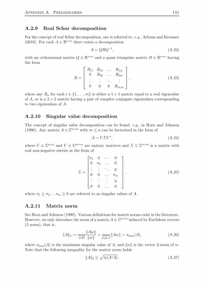
Appendix A. Preliminaries 141
A.2.9 Real Schur decomposition
For the concept of real Schur decomposition, one is referred to, e.g., Arbenz and Kressner(2010). For each A ∈ Rn×n there exists a decomposition
A = QRQ−1, (A.22)
with an orthonormal matrix Q ∈ Rn×n and a quasi triangular matrix R ∈ Rn×n havingthe form
R =
R11 R12 . . . R1m
0 R22 . . . R2m...
.... . .
...0 0 0 Rm,m
, (A.23)
where any Rii for each i ∈ 1, . . . ,m is either a 1× 1 matrix equal to a real eigenvalueof A, or is a 2× 2 matrix having a pair of complex conjugate eigenvalues correspondingto two eigenvalues of A.
A.2.10 Singular value decomposition
The concept of singular value decomposition can be found, e.g., in Horn and Johnson(1990). Any matrix A ∈ Cn×m with m ≤ n can be factorized in the form of
A = UΣV ∗, (A.24)
where U ∈ Cn×n and V ∈ Cm×m are unitary matrices and Σ ∈ Cn×m is a matrix withreal non-negative entries in the form of
Σ =
σ1 0 · · · 00 σ2 . . . 0...
.... . . 0
0 0 . . . σm...
...... 0
0 0 . . . 0
, (A.25)
where σ1 ≥ σ2 . . . σm ≥ 0 are referred to as singular values of A.
A.2.11 Matrix norm
See Horn and Johnson (1990). Various definitions for matrix norms exist in the literature.However, we only introduce the norm of a matrix A ∈ Cn×m induced by Euclidean vectors(2 norm), that is,
‖A‖2 := maxw 6=0
‖Aw‖‖w‖ = max
‖w‖=1‖Aw‖ = σmax(A), (A.26)
where σmax(A) is the maximum singular value of A, and ‖w‖ is the vector 2-norm of w.Note that the following inequality for the matrix norm holds
‖A‖2 ≤√
tr(A∗A). (A.27)
142 A.3. Controlled linear systems
A.2.12 Similarity
The definition of similarity can be found, for example, in Horn and Johnson (1990). Twomatrices A ∈ Cn×n and A ∈ Cn×n are similar if there exists an invertible matrix T suchthat
A = T−1AT. (A.28)
A.2.13 Invariant subspace of a matrix
This information can be found, for example, in Gohberg et al. (2006). An m dimensionalsubspace Xm of Cn is said to be A invariant if for each v ∈ Xm, we have Av ∈ Xm. Letthe columns of V = [v1 . . . , vm] be a basis for Xm, then there exists a matrix L ∈ Cm×m,such that
AV = V L. (A.29)
Moreover, the set of eigenvalues of L is a subset of the set of eigenvalues of A.
A.2.13.1 Distance between subspaces
For this part we refer the readers to Truhar (1996). Let Vi and Vj for some i, j ∈ Nbe bases for the two m dimensional subspaces Xi,m and Xj,m, respectively. Define theorthogonal projection matrices PXi,m = Vi(V
∗i Vi)
−1V ∗i and PXj,m = Vj(V∗j Vj)
−1V ∗j . Then,the distance between the two m dimensional subspaces Xi,m and Xj,m is defined by thenorm of the difference between the corresponding orthogonal projection matrices
dist(Xi,m,Xj,m) := ‖PXi,m − PXj,m‖.
Moreover, we have‖PXi,m − PXj,m‖ = sin θij,
where θij is the greatest canonical angle between Xi,m and Xj,m which is defined by
cos θij = minx∈Xi,mx6=0
maxy∈Xj,my 6=0
y∗x
‖x‖‖y‖ . (A.30)
A.3 Controlled linear systems
Consider an LTI system
x = Ax+Bu, (A.31)
where A ∈ Cn×n and B ∈ Cn×m. The controllability matrix Φc(A,B) for this system isdefined by
Φc(A,B) = [B AB . . . An−1B]. (A.32)
The pair (A,B) is said to be controllable if rank(Φc(A,B)) = n.
Appendix A. Preliminaries 143
A.3.1 [A B] invariant subspace
This part is taken from Gohberg et al. (2006). An m dimensional subspace Xm of Cn issaid to be [A B] invariant, if there exists a matrix F ∈ Rn×m such that for each ν ∈ Xm,(A + BF )ν ∈ Xm. When F = 0, this is interpreted as the familiar relation AXm ⊆ Xm,for A invariant subspace Xm.
A.3.2 Controlled block similarity
This definition has been taken from Gohberg et al. (2006). We say two controlled pairs[A B] ∈ Cn×n × Cn×m and [A B] ∈ Cn×n × Cn×m are block similar, if there exists aninvertible transformation matrix S ∈ C(m+n)×(m+n) in the form of
S =
[N 0L M
], (A.33)
such that
[A B] = N−1[A B]
[N 0L M
]. (A.34)
A.4 Input/Output linear systems
Consider an LTI system x = Ax+Bu,
y = Cx+Du,(A.35)
where A ∈ Cn×n, B ∈ Cn×m, C ∈ Cm×n, and D ∈ Cm×m. The observability matrix isdefined by
Φo(C,A) =
C
CA...
CAn−1
. (A.36)
Then, (C,A) is called observable if rank (Φo(C,A)) = n; see Kailath (1980). The transferfunction matrix of the system (A.35) equals
G(s) = C(sI − A)−1B +D. (A.37)
We say (A,B,C,D) is a realization of the transfer function matrix G(s). This realizationis minimal if and only if (A,B) is controllable and (C,A) is observable.
144 A.5. Linear time varying systems
A.4.1 Kalman-Yakubovic-Popov (KYP) lemma
The KYP lemma gives algebraic conditions for the existence of a certain type of Lyapunovfunctions for strictly positive real systems; see Boyd et al. (1994), and Zhou et al. (1996).
Lemma A.4.1. Consider the LTI system (A.35). Let A ∈ Rn×n be Hurwitz, B ∈ Rn×m,C ∈ Rm×n, D ∈ Rm×m, (A,B) be controllable, and (C,A) be observable. Then, thetransfer function matrix G(s) = C(sI −A)−1B +D is strictly positive real if and only ifthere exist matrices P = P> > 0, matrices L and W , and a number α > 0, satisfying
A>P + PA = −L>L− αP, (A.38)
B>P +W>L = C, (A.39)
D +D> = W>W. (A.40)
A.5 Linear time varying systems
The concept of solutions for linear time varying systems can be found, for instance, in(Kailath, 1980). Consider the linear time varying system
x = A(t)x(t) +B(t)u(t) x(t0) = x0. (A.41)
The solution to this system is given by
x(t) = φ(t, t0)x0 +
∫ t
t0
φ(t, τ)B(τ)u(τ) dτ. (A.42)
In this representation, φ is called state transition matrix and satisfies the conditions
∂φ(t, t0)
∂t= A(t)φ(t, t0), (A.43)
φ(τ, τ) = I. (A.44)
A.6 Differential equations and inclusions
Here, we summarize some important concepts concerning the theory of differentialequations and inclusions. They can be found, for example, in Cortes (2008); Smirnov(2001).
A.6.1 Absolute continuity
The function γ : [a, b] → R is absolutely continuous in the interval [a, b], if there existsa Lebesgue integral function k : [a, b]→ R such that
γ(t) = γ(a) +
∫ t
a
k(τ) dτ t ∈ [a, b]. (A.45)

Appendix A. Preliminaries 145
Absolute continuity is a stronger notion than continuity and weaker than differentiabil-ity. Every continuous differentiable function is absolutely continuous, but the inverseis not true. However, every absolutely continuous function is differentiable almosteverywhere.
A.6.2 Solutions of differential equations
For a definition of the different classes of solutions for differential equations see, e.g.,Cortes (2008). Consider the differential equation
x = f(x(t)) x(t0) = x0, (A.46)
where f : Rn → Rn represents the direction of the vector field at each point x. If f iscontinuous, then the solutions to (A.46) are continuously differentiable. These solutionsare called classical solutions. If f is not continuous, then different notions of solutions fordifferential equation (A.46) are defined. In the following, we point out couple of them.
A.6.2.1 Caratheodory solutions
See Cortes (2008). Caratheodory solutions are absolutely continuous solutions x(t),which result from integrating (A.46)
x(t) = x(t0) +
∫ t
t0
f(x(τ)) dτ. (A.47)
Caratheodory solutions may not always follow the direction of vector fields, for example,at points of measure zero.
A.6.2.2 Filippov solutions
See Cortes (2008) and Filippov (1988). The Filippov set valued map considers thedirections of vector fields around any point in the state space. For defining the Filippovsolutions, the vector field in the right hand side of (A.46) is replaced by the so-calledFilippov set-valued map defined by
F (x) :=⋂δ>0
⋂µ(S)=0
co f(B(x, δ)\S), (A.48)
where co denotes the convex closure and µ denotes the Lebesgue measure. Then, theFilippov solutions are solutions of the following differential equations
x ∈ F (x). (A.49)
For instance, the differential equation
x =
1 x ≥ 0,−1 x < 0,

146 A.7. Hybrid systems
is modified to the differential inclusion defined by
x ∈
1 x > 0,
[−1, 1] x = 0,
−1 x < 0.
Consider a differential inclusion x ∈ F (x). In the theory of differential inclusions,often some restrictions on set valued map F are assumed. We explain some relatedconcepts; See Cai et al. (2008) and Goebel et al. (2012).
A.6.3 Outer semi-continuous set valued map
A set valued map F : Rn → 2Rn is said to be outer semi-continuous at the point x, if
limx→x
sup F (x) ⊂ F (x). (A.50)
A.6.4 Convex set valued map
A set valued map F : Rn → 2Rn is said to be convex, if the set is convex for all x. Inother words, for each x0, x1 ∈ Rn
F ((1− α)x0 + αx1) ⊃ (1− α)F (x0) + αF (x1) ∀ α ∈ [0, 1]. (A.51)
A.6.5 Locally bounded set valued map
A set valued map F : Rn → 2Rn is said to be locally bounded at the point x, if for someneighborhood N (x), for each V ∈ N (x) the set F (V ) ⊂ Rn is bounded. It is calledlocally bounded on Rn if it is locally bounded at every point x ∈ Rn.
A.7 Hybrid systems
Consider a hybrid system described by the four tuples (C,F,D,G), i.e., a differentialand a difference inclusion in the form of
H :
x ∈ F (x) x ∈ C,x+ ∈ G(x) x ∈ D.
(A.52)
The sets C and D are referred to as flow and jump sets, respectively. Typically, it isassumed that the set valued map F : C → 2Rn , which contains the set of all possible flowdirections within the closed set C, is nonempty, convex, and outer semi-continuous. Theset valued map G : D → 2Rn , which represents the set-valued jump function, is assumedto be nonempty and outer semi-continuous. These assumptions on H are called “basicassumptions”; see Goebel et al. (2012).

Appendix A. Preliminaries 147
A.7.1 Perturbed hybrid systems
Given a hybrid system (A.52) and a continuous function δ : Rn → R≥0, the hybridsystem Hδ described by the four tuple (Cδ, Fδ, Dδ, Gδ) and
Hδ :
x ∈ Fδ(x) x ∈ Cδ,x+ ∈ Gδ(x) x ∈ Dδ,
(A.53)
with the data
Cδ := x : (x+ δ(x)B) ∩ C 6= ∅,Fδ(x) := co F ((x+ δ(x)B) ∩ C) + δ(x)B ∀x ∈ Cδ,Dδ := x : (x+ δ(x)B) ∩D 6= ∅,Gδ(x) := v : v ∈ g + δ(g)B, g ∈ G((x+ δ(x)B) ∩D) ∀ x ∈ Dδ, (A.54)
is called the perturbed form of H with respect to the uncertainty function δ. In thisform, B denotes the closed unit ball and the uncertainty δ is typically a continuousfunction.
A function α : R≥0 → R≥0 is said to be increasing positive definite or belong to theclass K∞, if it is continuous, zero at zero, and strictly increasing. We make use of thefollowing theorems, concerning robust stability of the hybrid system H or stability ofthe perturbed hybrid system Hδ.
Theorem A.7.1. See Cai et al. (2008) and Goebel et al. (2012). Consider the hybridsystem H defined by (A.52) satisfying the basic assumptions and C∪D = Rn. Suppose acompact set A ⊂ Rn exists such that G(D ∩ A) ⊂ A. If there exists a smooth Lyapunovfunction V : Rn → R≥0 for the pair (H,A), that is, V is positive on (C ∪ D)\A,limx→A V (x) = 0, and
〈∇V (x), f〉 < 0 x ∈ C\A, f ∈ F (x)
V (g)− V (x) < 0 x ∈ D\A, g ∈ G(x)\A,(A.55)
then the set A is asymptotically stable, and the basin of attraction contains every forwardinvariant compact set.
Theorem A.7.2. See Cai et al. (2008) and Goebel et al. (2012). Consider the hybridsystem H defined by (A.52). If the compact set A is globally asymptotically stable, thenthere exist a smooth function V : Rn → R≥0, and α1, α2 ∈ K∞, such that
α1(‖x‖A)) ≤ V (x) ≤ α2(‖x‖A) ∀x ∈ Rn,
maxf∈F (x)
〈∇V (x), f〉 ≤ −V (x), ∀x ∈ C,
maxg∈G(x)
V (g) ≤ e−1V (x) ∀x ∈ D,(A.56)
where ‖x‖A denotes infy∈A(‖x − y‖). Moreover, the set A is asymptotically stablefor the perturbed hybrid system Hδ = (Cδ, Fδ, Dδ, Gδ) with some continuous functionδ : Rn → Rn
≥0, where δ(x) is positive for x ∈ (C ∪D) \A .

148 A.8. Optimization
A particular case of Theorem A.7.2 is obtained by assigning D = ∅ and C = Rn. Inthis case,
Fδ(x) := co F (x+ δ(x)B) + δ(x)B ∀x ∈ Rn, (A.57)
and the equations (A.56) concerning the Lyapunov function will be modified to
α1(‖x‖A)) ≤ V (x) ≤ α2(‖x‖A),
maxf∈F (x)
〈∇V (x), f〉 ≤ −V (x); (A.58)
see Teel and Praly (2000). We use the former description for robust stability of hybridsystems, and the latter illustration for robust stability of switched linear systems.
A.8 Optimization
Now, we present some basic concepts of optimization.
A.8.1 Projection onto a linear subspace
See Boyd and Vandenberghe (2004). The projection of a point x0 onto the set
X = x ∈ Rn : Ax− b = 0,denoted by ProjX (x0), equals
ProjX (x0) = x0 − A>(AA>)−1(Ax0 − b). (A.59)
A.8.2 Hamilton-Jacobi-Bellman equation
See, e.g., Lewis and Syrmos (1995). Consider the following problem
J(x(0), 0) = minu
∫ T
0
C(x(t), u(t)) dt+D (x(T ))
(A.60)
subject to x(t) = f(x(t), u(t)), (A.61)
where C[.] is the scalar cost function, D[.] is a function that specifies the cost at thefinal state x(T ), x(t) is the system state vector, x(0) is assumed to be given, and u(t)for 0 ≤ t ≤ T is the control input vector that must be computed. For this problem, theHamilton Jacobi Bellman partial differential equation is defined by
J(x, t) + minu∇J(x, t) · f(x, u) + C(x, u) = 0, (A.62)
subject to the terminal condition
J(x, T ) = D(x), (A.63)
where ∇ is the gradient operator.

Appendix A. Preliminaries 149
A.8.3 Optimal control with fixed time and fixed final state incontinuous time
See Lewis and Syrmos (1995) and Bryson and Ho (1975). Consider the optimal controlproblem
J(t0) =1
2x(T )> S(T ) x(T ) +
1
2
∫ T
t0
(x> Q x+ u> R u) dt, (A.64)
subject to
x = Ax+Bu t ≥ t0,
x(t0) = x0,
C x(T ) = r,
(A.65)
with the given initial condition x0, final time T , S(T ) ≥ 0, Q ≥ 0, R > 0, the matrixC, and the vector r. Then, the optimal control law which minimizes the cost (A.64) isgiven as follows:
u(t) = −(K(t)−R−1B>V (t)P (t)−1V (t)>
)x−R−1B>V (t)P (t)−1 r(T ), (A.66)
where
−S = A>S + SA− SBR−1B>S +Q,
K = R−1B>S,
−V = (A−BK)>V t ≤ T,
P = V >BR−1B>V t ≤ T, (A.67)
and the following boundary conditions hold
V (T ) = C>, P (T ) = 0, S(T ) ≥ 0 is given.
If det(P (t)) = 0 for all t ∈ (t0, T ), the problem is said to be abnormal and there is nosolution. Note that the parameter
θ := P (t)−1(r(T )− V (t)>x(t)
), (A.68)
is fixed for any t ∈ [0, T ], where det(P (t)) 6= 0.
A.8.4 Optimal control with fixed time and fixed final state indiscrete time
See Lewis and Syrmos (1995). Consider the optimization problem
J =1
2x>K SK xK +
1
2
K−1∑k=i
[x>k Q xk + u>k R uk], (A.69)
subject to
x+ = Axk +Buk k > i,
xi given,
C xK = rK ,

150 A.8. Optimization
with the given final time K, SK ≥ 0, Q ≥ 0, R > 0, the matrix C, and the vector rK .Then, the optimal control is given by
uk = −Kk xk +Kuk Vk+1 P
−1k [V >k xk − rK ], (A.70)
where
Kk = (B> Sk+1 B +R)−1 B> Sk+1 A,
Sk = A> Sk+1 (A−BKk) +Q,
Vk = (A−B Kk)>Vk+1,
Pk = Pk+1 − V >k+1 B (B> Sk+1 B +R)−1 B> Vk+1,
Kuk = (B> Sk+1 B +R)−1 B>, (A.71)
with the boundary conditions
VK = C>, PK = 0, SK ≥ 0 is given.
If det(Pi) = 0 for all i ≤ k ≤ K, the problem has no solution in the interval i, i +1, . . . , K. In this case the problem is said to be abnormal. Note that the parameter
θ = P−1k (rK − V >k xk), (A.72)
is fixed for any k ∈ i, i+ 1, . . . , K, where det(Pk) 6= 0.

BIBLIOGRAPHY 151
Bibliography
A. A. Agrachev and D. Liberzon. Lie-algebraic stability criteria for switched systems.SIAM Journal on Control and Optimization, 40(1):253–269, 2001.
A. Ahmadi, R. Jungers, P. Parrilo, and M. Roozbehani. Joint spectral radius and path-complete graph Lyapunov functions. SIAM Journal on Control and Optimization, 52(1):687–717, 2014.
P. Arbenz and D. Kressner. Lecture Notes on Solving Large Scale Eigenvalue Problems.2010.
V. Azhmyakov, S. A. Attia, D. Gromov, and J. Raisch. Necessary optimality conditionsfor a class of hybrid optimal control problems. In Hybrid Systems: Computation andControl, volume 4416 of Lecture Notes in Computer Science, pages 637–640. Springer,2007.
V. Azhmyakov, R. Galvan-Guerra, and M. Egerstedt. Hybrid LQ-optimization usingdynamic programming. In Proc. of the American Control Conference, pages 3617–3623, 2009.
N. Bajcinca and M. Voigt. Spectral conditions for symmetric positive real and negativeimaginary systems. In Proc. of the European Control Conference, pages 809–814, 2013.
N. Bajcinca, D. Flockerzi, and Y. Kouhi. On a geometrical approach to quadraticLyapunov stability and robustness. In Proc. of the 52th Conference on Decision andControl, pages 1–6, 2013.
G. Balas, J. Bokor, and Z. Szabo. Invariant subspaces for LPV systems and their appli-cations. IEEE Transactions on Automatic Control, 48(11):2065–2069, 2003.
N. Barabanov. Lyapunov exponent and joint spectral radius: some known and newresults. In Proc. of the 44th IEEE Conference on Decision and Control and EuropeanControl Conference, pages 2332–2337, 2005.
L. Bayon, J. M. Grau, M. M. Ruiz, and P. M. Suarez. An analytic solution for someseparable convex quadratic programming problems with equality and inequality con-straints. Journal of Mathematical inequalities, 4(2):453–465, 2010.
F. Blanchini. Set invariance in control. Automatica, 35(11):1747–1767, 1999.
S. Boyd and L. Vandenberghe. Convex optimization. Cambridge University Press, 2004.

152 BIBLIOGRAPHY
S. Boyd, L. El Ghaoui, E. Feron, and V. Balakrishnan. Linear Matrix Inequalities inSystem and Control Theory, volume 15. PA: SIAM, 1994.
M. S. Branicky. Multiple Lyapunov functions and other analysis tools for switched andhybrid systems. IEEE Transactions on Automatic Control, 43(4):475–482, 1998.
B. Brogliato. Nonsmooth Mechanics: Models, Dynamics and Control. Springer-Verlag,New York, 1999.
A. E. Bryson and Y. C. Ho. Applied optimal control. Hemisphere, New York, 1975.
C. Cai, A. R. Teel, and R. Goebel. Smooth Lyapunov functions for hybrid systems-Part I:Existence is equivalent to robustness. IEEE Transactions on Automatic Control, 52(7):1264–1277, 2007.
C. Cai, A. R. Teel, and R. Goebel. Smooth Lyapunov functions for hybrid systemsPart II: (pre)asymptotically stable compact sets. IEEE Transactions on AutomaticControl, 53(3):734–748, 2008.
P. E. Caines, F. H. Clarke, X. Lie, and R. B. Vinter. A maximum principle for hybridoptimal control problems with pathwise state constraints. In Proc. of the 45th IEEEConference on Decision and Control, pages 4821–4825, 2006.
D. Cheng. Stabilization of planar switched systems. Systems and Control Letters, 51(2):79–88, 2004.
G. Chesi, P. Colaneri, J. C. Geromel, R. Middleton, and R. Shorten. A nonconservativeLMI condition for stability of switched systems with guaranteed dwell time. IEEETransactions on Automatic Control, 57(5):1297–1302, 2012.
J. W. Choi. Left eigenstructure assignment via sylvester equation. Journal of MechanicalScience and Technology, 12(6):1034–1040, 1998a.
J. W. Choi. A simultaneous assignment methodology of right/left eigenstructures. IEEETransactions on Aerospace and Electronic Systems, 34(2):625–634, 1998b.
F. H. Clarke, Y. S. Ledyaev, E. D. Sontag, and A. I. Subbotin. Asymptotic controllabilityimplies feedback stabilization. IEEE Transactions on Automatic Control, 42(10):1394–1407, 1997.
E. A. Coddington and N. Levinson. Theory of Ordinary Differential Equations. NewYork: McGraw-Hill, 1955.
M. Corless and R. Shorten. On the characterization of strict positive realness for generalmatrix transfer functions. IEEE Transactions on Automatic Control, 55(8):1899–1904,2010.
J. Cortes. Discontinuous dynamical systems: A tutorial on solutions, nonsmooth analysisand stability. IEEE Control Systems Magazine, 28(3):36–73, 2008.
T. Craven and G. Csordas. A sufficient condition for strict total positivity of a matrix.Linear Multilinear Algebra, 45(2):19–34, 1998.
BIBLIOGRAPHY 153
J. Daafouz, P. Riedinger, and C. Iung. Stability analysis and control synthesis forswitched systems: a switched Lyapunov function approach. IEEE Transactions onAutomatic Control, 47(11):1883–1887, 2002.
B. De Schutter and W. P. M. H. Heemels. Modeling and control of hybrid systems.Lecture notes of the DISC course, 2004.
D. K. Dimitrov and J. M. Pena. Almost strict total positivity and a class of Hurwitzpolynomials. Journal of Approximation Theory, 132(2):212–223, 2005.
F. El Hachemi, M. Sigalotti, and J. Daafouz. Stability of planar singularly perturbedswitched systems. In Proc. of the American Control Conference (ACC), 2011, pages1464–1469, 2011.
E. Feron. Quadratic stabilizability of switched systems via state and output feedback.Technical report, Center for Intelligent Control Systems, MIT, Cambridge, MA, 1996.
A. F. Filippov. Differential equations with discontinuous righthand sides: Control Sys-tems (Mathematics and its Applications). Springer, 1st edition, 1988.
E. Fornasini and M. E. Valcher. On the stability of continuous-time positive switchedsystems. In Proc. of the American Control Conference (ACC), 2010, pages 6225–6230,2010.
P. A. Fuhrmann. On symmetric rational transfer functions. Linear Algebra and itsApplications, 50(0):167–250, 1983.
J. Geromel and P. Colaneri. Stability and stabilization of continuous time switched linearsystems. SIAM Journal on Control and Optimization, 45(5):1915–1930, 2006.
R. Goebel, R. G. Sanfelice, and A. Teel. Hybrid dynamical systems. IEEE ControlSystems Magazine, 29(2):28–93, 2009.
R. Goebel, R. G. Sanfelice, and A. R. Teel. Hybrid Dynamical Systems: Modeling,Stability, and Robustness. Princeton University Press, New Jersey, 2012.
I. Gohberg, P. Lancaster, and L. Rodman. Invariant Subspaces of Matrices with Appli-cations. Society for Industrial and Applied Mathematics, 2006.
W. M. Griggs, C. K. King, R. Shorten, O. Mason, and K. Wulff. Quadratic Lyapunovfunctions for systems with state-dependent switching. Linear Algebra and its Appli-cations, 433(1):52– 63, 2010.
H. Haimovich and J. H. Braslavsky. Feedback stabilisation of switched systems viaiterative approximate eigenvector assignment. In Proc. of the 49th Conference onDecision and Control, pages 1269–1274, 2010.
W. P. M. H. Heemels, D. Lehmann, J. Lunze, and B. De Schutter. Handbook of HybridSystems Control. Cambridge University Press, 2009.
U. Helmke, J. Rosenthal, and X. A. Wang. Output feedback pole assignment for transferfunctions with symmetries. SIAM J. of Control and Optimization, 45(5):1898–1914,2006.

154 BIBLIOGRAPHY
J. P. Hespanha and A. S. Morse. Stability of switched systems with average dwell-time. In Proc. of the 38th IEEE Conference on Decision and Control, volume 3, pages2655–2660, 1999.
R. A. Horn and C. R. Johnson. Matrix Analysis. Cambridge University Press, 1990.
M. Hovd and S. Skogestad. Control of symmetrically interconnected plants. Automatica,30(6):957–973, 1994.
C. H. Huang, P. A. Ioannou, J. Maroulas, and M. G. Safonov. Design of strictly pos-itive real systems using constant output feedback. IEEE Transactions on AutomaticControl, 44(3):569–573, 1999.
T. A. Johansen, I. Petersen, and O. Slupphaug. Explicit suboptimal linear quadraticregulation with state and input constraints. Automatica, 38(7):1099–1111, 2002.
A. A. Julius and A. J. Van der Schaft. The maximal controlled invariant set of switchedlinear systems. In Proc. of the 41st IEEE Conference on Decision and Control, vol-ume 3, pages 3174–3179, 2002.
T. Kailath. Linear Systems. Prentice Hall, Englewood Cliffs, NJ, 1980.
O. M. Katkova and A. M. Vishnyakova. A sufficient condition for a polynomial to bestable. Journal of Mathematical Analysis and Applications, 347(1), 2008.
H. Khalil. Nonlinear Systems. Prentice Hall, 2002.
C. King and M. Nathanson. On the existence of a common quadratic Lyapunov functionfor a rank one difference. Linear Algebra and its Applications, 419(2–3):400–416, 2006.
L. Knockaert, F. Ferranti, and T. Dhaene. Generalized eigenvalue passivity assessment ofdescriptor systems with applications to symmetric and singular systems. InternationalJournal of Numerical Modeling: Electronic Networks, Devices and Fields, 26(1):1–14,2013.
Y. Kouhi and N. Bajcinca. On the left eigenstructure assignment and state feedbackdesign. In Proc. of the American Control Conference, pages 4326–4327, 2011a.
Y. Kouhi and N. Bajcinca. Nonsmooth control design for stabilizing switched linearsystems by left eigenstructure assignment. In Proc. of the IFAC World Congress,pages 380–385, 2011b.
Y. Kouhi and N. Bajcinca. Robust control of switched linear systems. In Proc. of the50th IEEE Conference on Decision and Control and European Control Conference,pages 4735–4740, 2011c.
Y. Kouhi, N. Bajcinca, J. Raisch, and R. Shorten. A new stability result for switchedlinear systems. In Proc. of the European Control Conference, pages 2152–2156, 2013a.
Y. Kouhi, N. Bajcinca, and R. G. Sanfelice. Suboptimality bounds for linear quadraticproblems in hybrid linear systems. In Proc. of the European Control Conference, pages2663–2668, 2013b.

BIBLIOGRAPHY 155
Y. Kouhi, N. Bajcinca, J. Raisch, and R. Shorten. On the quadratic stability of switchedlinear systems associated with symmetric transfer function matrices. Automatica, 50(11):2872–2879, 2014.
T. J. Laffey. Common Lyapunov solutions for two matrices whose difference has rankone. Linear Algebra and its Applications, 431(1–2):228–240, 2009.
C. H. Lee. New results for the bounds of the solution for the continuous Riccati andLyapunov equations. IEEE Transactions on Automatic Control, 42(1):118–123, 1997.
F. L. Lewis and V. L. Syrmos. Optimal Control. John Wiley and Sons, 2nd edition,1995.
D. Liberzon. Calculus of variations and optimal control theory: A concise introduction.Princeton University Press, 2011.
D. Liberzon, J. P. Hespanha, and A. S. Morse. Stability of switched systems: a Lie-algebraic condition. Systems and Control Letters, 37(3):117–122, 1999.
H. Lin and P. J. Antsaklis. Stability and stabilizability of switched linear systems: Asurvey of recent results. IEEE Transactions on Automatic Control, 54(2):308–322,2009.
G. P. Liu and R. J. Patton. Eigenstructure Assignment for Control System Design. JohnWiley and Sons, 1998.
J. Lygeros. Lecture notes on hybrid systems. 2004.
O. Mason and R. Shorten. On common quadratic Lyapunov functions for stable discretetime LTI systems. IMA Journal of Applied Mathematics, 69(3):271–283, 2004.
A. P. Molchanov and Ye. S. Pyatnitskiy. Criteria of asymptotic stability of differentialand difference inclusions encountered in control theory. Systems and Control Letters,13(1):59–64, 1989.
K. S. Narendra and J. Balakrishnan. A common Lyapunov function for stable LTIsystems with commuting A-matrices. IEEE Transactions on Automatic Control, 39(12):2469–2471, 1994.
K. S. Narendra and J. H. Taylor. Frequency domain criteria for absolute stability. Aca-demic Press Inc., 1973.
J. Nocedal and S. Wright. Numerical Optimization. Springer, 2nd edition, 2006.
R. Olfati-Saber and R. M. Murray. Consensus problems in networks of agents withswitching topology and time-delays. IEEE Transactions on Automatic Control, 49(9):1520–1533, 2004.
B. Passenberg, M. Leibold, O. Stursberg, and M. Buss. The minimum principle fortime-varying hybrid systems with state switching and jumps. In Proc. of the 50thIEEE Conference on Decision and Control and European Control Conference, pages6723–6729, 2011.

156 BIBLIOGRAPHY
J. Raisch, E. Klein, C. Meder, A. Itigin, and S. O Young. Approximating automataand discrete control for continuous systems - two examples from process control. InHybrid Systems V, volume 1567 of Lecture Notes in Computer Science, pages 279–303.Springer Berlin Heidelberg, 1999.
A. Rantzer and M. Johansson. Piecewise linear quadratic optimal control. IEEE Trans-actions on Automatic Control, 45(2):629–637, 2000.
W. Ren and R. W. Beard. Distributed Consensus in Multi-vehicle Cooperative Control:Theory and Applications. Springer Publishing Company, 2007.
P. Riedinger, F. Kratz, C. Iung, and C. Zanne. Linear quadratic optimization for hybridsystems. In Proc. of the 38th IEEE Conference on Decision and Control, volume 3,pages 3059–3064, 1999.
F. Rossi, P. Colaneri, and R. Shorten. Pade discretization for linear systems with polyhe-dral Lyapunov functions. IEEE Transactions on Automatic Control, 56(11):2717–2722,2011.
Y. Saad. A projection method for partial pole assignment in linear state feedback.Technical Report 449, YALEU/DCS, 1986.
J. Schiffer, A. Anta, T. D. Trung, J. Raisch, and T. Sezi. On power sharing and stabilityin autonomous inverter-based microgrids. In Proc. of the 51st IEEE Conference onDecision and Control, pages 1105–1110, 2012.
A. Semlyen and B. Gustavsen. A half-size singularity test matrix for fast and reliablepassivity assessment of rational models. IEEE Transactions on Power Delivery, 24(1):345–351, 2009.
F. G. Shinskey. Distillation Control. McGraw-Hill, 1984.
R. Shorten and F. O. Cairbre. On the stability of pairwise triangularisable and relatedswitching systems. In Proc. of the American Control Conference, volume 3, pages1882–1883, 2001.
R. Shorten and K. S. Narendra. On the stability and existence of common Lyapunovfunctions for stable linear switching systems. In Proc. of the 37th IEEE Conferenceon Decision and Control, volume 4, pages 3723–3724, 1998.
R. Shorten and K. S. Narendra. Necessary and sufficient conditions for the existenceof a common quadratic Lyapunov function for a finite number of stable second orderlinear time-invariant systems. International Journal of Adaptive Control and SignalProcessing, 16(10):709–728, 2002.
R. Shorten and K. S. Narendra. On common quadratic Lyapunov functions for pairs ofstable LTI systems whose system matrices are in companion form. IEEE Transactionson Automatic Control, 48(4):618–621, 2003.
R. Shorten, F. Wirth, K. Wulff, and C. King. Stability criteria for switched and hybridsystems. SIAM, 49(4):545–592, 2007.

BIBLIOGRAPHY 157
R. Shorten, P. Curran, K. Wulff, and E. Zeheb. A note on spectral conditions for positiverealness of transfer function matrices. IEEE Transactions on Automatic Control, 53(5):1258–1261, 2008.
R. Shorten, M. Corless, K. Wulff, S. Klinge, and R. Middleton. Quadratic stability andsingular SISO switching systems. IEEE Transactions on Automatic Control, 54(11):2714–2718, 2009.
I. Simeonova. On-line periodic scheduling of hybrid chemical plants with parallel pro-duction lines and shared resources. PhD thesis at Universite catholique de Louvain,2008.
I. Simeonova, F. Warichet, G. Bastin, D. Dochain, and Y. Pochet. Feedback stabilizationof the operation of an hybrid chemical plant. In Proc. of the 2nd IFAC Conference onAnalysis and Design of Hybrid Systems, pages 191–198, 2006.
J. D. Simon and S. K. Mitter. A theory of modal control. Information and Control, 13(4):316–353, 1968.
H. Sira-Ramirez. A geometric approach to pulse-width modulated control in nonlineardynamical systems. IEEE Transactions on Automatic Control, 34(2):184–187, 1989.
G. Smirnov. Introduction to the Theory of Differential Inclusions (Graduate Studies inMathematics). American Mathematical Society, 1st edition, 2001.
V. Solo. On the stability of slowly time-varying linear systems. Mathematics of Control,Signals and Systems, 7(4):331–350, 1994.
G. W. Stewart. Matrix Algorithms, Volume II: Eigensystems. SIAM, 2001.
Z. Sun and D. Zheng. On reachability and stabilization of switched linear systems. IEEETransactions on Automatic Control, 46(2):291–295, 2001.
H. J. Sussmann. A maximum principle for hybrid optimal control problems. In Proc. ofthe 38th IEEE Conference on Decision and Control, pages 425–430, 1999.
A. Teel and L. Praly. A smooth Lyapunov function from a class-KL estimate involvingtwo positive semidefinite functions. ESAIM: Control, Optimisation and Calculus ofVariations, pages 313–367, 2000.
N. Truhar. Perturbation of invariant subspaces. Lecture presented at the MathematicalCOLLOQUIUM, 1996.
M. Tsatsomeros. A criterion for the existence of common invariant subspace of matrices.Linear Algebra and its Applications, pages 51–59, 2001.
M. Wicks, P. Peleties, and R. DeCarlo. Switched controller synthesis for the quadraticstabilization of a pair of unstable linear systems. European Journal of Control, 4(2):140–147, 1998.
J. C. Willems. Dissipative dynamical systems Part II: Linear systems with quadraticsupply rates. Archive for Rational Mechanics and Analysis, 45(5):352–393, 1972.

158 BIBLIOGRAPHY
F. Wirth. A converse Lyapunov theorem for linear parameter varying and linear switchingsystems. SIAM Journal on Control and Optimization, 44(1):210–239, 2005a.
F. Wirth. The generalized spectral radius is strictly increasing. Linear Algebra and itsApplications, 395(0):141–153, 2005b.
W. M. Wonham. On pole assignment in multi-input controllable linear systems. IEEETransactions on Automatic Control, 12(6):660–665, 1967.
K. Wulff. Quadratic and non-quadratic stability criteria for switched linear systems. PhDthesis, Hamilton Institute, NUI Maynooth, 2005.
G. Xie, Q. Fu, and L. Wang. Stabilization of switched symmetric systems. In Proc. ofthe American Control Conference, volume 5, pages 4535–4536, 2004.
X. Xu and P. J. Antsaklis. Optimal control of switched systems based on parameter-ization of the switching instants. IEEE Transactions on Automatic Control, 49(1):637–640, 2004.
G. H. Yang and L. Qiu. Optimal symmetric H2 controllers for systems with collocatedsensors and actuators. IEEE Transactions on Automatic Control, 47(12):2121–2125,2002.
E. Yurtseven, W. P. M. H. Heemels, and M. K. Camlibel. Disturbance decouplingof switched linear systems. In Proc. of the 49th IEEE Conference on Decision andControl, pages 6475–6480, 2010.
K. Zhou, J. C. Doyle, and K. Glover. Robust and optimal control. Prentice Hall, UpperSaddle River, 1996.