Contributed article

A fast neural-network algorithm for VLSI cell placement

Cevdet Aykanata,*, Tevfik Bultanb, Ismail Haritaog˘lub

aDepartment of Computer Engineering, Bilkent University, Ankara, TR-06533, TurkeybDepartment of Computer Science, University of Maryland, College Park, MD 20742, USA

Received 4 July 1997; accepted 15 May 1998

Abstract

Cell placement is an important phase of current VLSI circuit design styles such as standard cell, gate array, and Field Programmable GateArray (FPGA). Although nondeterministic algorithms such as Simulated Annealing (SA) were successful in solving this problem, they areknown to be slow. In this paper, a neural network algorithm is proposed that produces solutions as good as SA in substantially less time. Thisalgorithm is based on Mean Field Annealing (MFA) technique, which was successfully applied to various combinatorial optimizationproblems. A MFA formulation for the cell placement problem is derived which can easily be applied to all VLSI design styles. Todemonstrate that the proposed algorithm is applicable in practice, a detailed formulation for the FPGA design style is derived, and thelayouts of several benchmark circuits are generated. The performance of the proposed cell placement algorithm is evaluated in comparisonwith commercial automated circuit design software Xilinx Automatic Place and Route (APR) which uses SA technique. Performanceevaluation is conducted using ACM/SIGDA Design Automation benchmark circuits. Experimental results indicate that the proposedMFA algorithm produces comparable results with APR. However, MFA is almost 20 times faster than APR on the average.q 1998 ElsevierScience Ltd. All rights reserved.

Keywords:VLSI circuit design; Cell placement problem; Field programmable gate array; Mean field annealing; Neural-network algorithms

1. Introduction

Cell placement is an important problem arising in variousVLSI circuit design styles such as standard cell, gate arrayand Field Programming Gate Array (FPGA). Given a circuitdescription, the problem is to find a layout of the circuitwhile minimizing some cost function. Usually two closelyrelated criteria are used to construct a cost function: mini-mization of the routing length and minimization of the chiparea. In some design styles (e.g. standard cell), minimizationof the area is equivalent to minimization of the routinglength (Shahookar and Mazumder, 1991), whereas insome others area is fixed (e.g. FPGA). If the area is fixed,minimization of the routing length is necessary for the rout-ability of the circuit using the available routing resources.Minimization of the routing length also minimizes the pro-pagation delays of the circuit, hence increasing its speed(Shahookar and Mazumder, 1991).

Although the cell placement problem has differentcharacteristics related to the technology used in differentdesign styles, key features of the problem remain the

same. This enables a general definition for the cellplacement problem to be made which is valid for all designstyles. The problem is decomposed into two phases suchthat the first phase is same for all design styles and thesecond phase depends on the design style. An instance ofthe first phase of the cell placement problem consists of ahypergraphQ(C, N) representing the circuit to be placed,and a rectangular grid of clusters withP rows andQcolumns where the circuit will be placed. HypergraphQ(C, N) consists of a vertex setC representing the cellsof the circuit, a hyperedge setN representing the nets of thecircuit, a cell weight functionqcell:C → N, and a net weightfunctionqnet:N → N, whereN represents the set of naturalnumbers. The aim is to partition the vertex setC into P 3 Qclusters such that the routing cost is minimized and theweights of the clusters are nearly balanced. The weightof a cluster is the sum of the weights of the cells in thatcluster. In general, cell weight function is used to encodethe areas of cells, and net weight function is used toincrease the importance of some nets which may be crucialfor the performance of the circuit. The rectangular grid ofclusters is used for estimating the final locations of thecells. The computation of routing cost is discussed in detailin Section 2.

* Corresponding author. Tel.: +90-312-266-4133; Fax: +90-312-266-4126; E-mail: aykanat@cs.bilkent.edu.tr

0893–6080/98/$ - see front matterq 1998 Elsevier Science Ltd. All rights reserved.PII: S0893-6080(98)00089-6

Neural Networks 11 (1998) 1671–1684PERGAMON

NeuralNetworks

Fig. 1(a) illustrates an example circuit with 16 cells and19 nets (Shahookar and Mazumder, 1991). The circuit has 3input (I1, I2, I3) and 2 output (O1, O2) pads. Pads may beinterpreted as cells which must be mapped to the boundariesof the cluster grid. The example circuit in Fig. 1(a) may berepresented with a hypergraphQ(C, N) according to theabove definition as:

C ¼{1, 2, 3, 4, 5, 6, 7, 8, 9, 10, 11, 12, 13, 14, 15, 16,I1, I2, I3, O1, O2}N ¼{{ I1, 1, 2, 3, 4}, {I2, 1, 2, 3, 4, 11, 12}, {I3, 6, 10, 11, 12, 13}, {1, 8},

{3, 7}, {11, 13}, {5, 6}, {8, 9}, {9, 15}, {13, 16}, { O1, 15}, {2, 5},{4, 10}, {12, 14}, {6, 8}, {7, 9}, {10, 15}, {14, 16}, { O2, 16}}

Unit cell and net weights are assumed in this example.Fig. 1(b) shows the placement of this circuit to a 43 4 gridof 16 clusters.

The second phase of the cell placement problem is themapping of the cells in the clusters to their final locations inthe layout. In standard cell design style, cells are used forconstructing rows, and in gate array design style, cells aremapped to rows or grid locations according to the type of thegate array used (Sechen, 1988). Some gate arrays consist ofmodules forming a rectangular grid. For this type of gatearrays the second phase of the problem may be skipped bychoosing the number of rows and columns of the cluster gridto be equal to the number of rows and columns of the mod-ule grid, respectively. Symmetrical FPGAs consist of logicblocks forming a rectangular grid (Rose et al., 1992, Rose etal., 1993). Hence, the second phase of the problem can besimilarly skipped for symmetrical FPGAs. This two phasemodeling enables the development of heuristics for the firstphase of the problem which are independent of the designstyle.

Since cell placement problem is NP-Hard (Lengauer,1990), finding efficient placement heuristics is an importantresearch issue. In the last decade, neurocomputingapproaches based on Hopfield model were successfullyapplied to various combinatorial optimization problemssuch as the traveling salesman problem (Peterson andSoderberg, 1989; VandenBout and Miller, 1989; Takahashi,1997), scheduling problem (Gisle´n et al., 1992), mappingproblem (Bultan and Aykanat, 1992), knapsack problem(Ohlsson et al., 1993; Ohlsson and Pi, 1997), communica-tion routing problem (Ho¨kkinen et al., 1998), graph parti-tioning problem (Herault and Niez, 1989; Peterson andSoderberg, 1989; VandenBout and Miller, 1990), graph lay-out problem (Cimikowski and Shope, 1996), circuit parti-tioning problem (Yih and Mazumder, 1990; Bultan andAykanat, 1995). In this paper, the Mean Field Annealing(MFA) technique is applied to the cell placement problem.MFA is a new approach for solving combinatorial optimiza-tion problems (Peterson and So¨derberg, 1989; VandenBoutand Miller, 1989, VandenBout and Miller, 1990; Gisle´n etal., 1992; Bultan and Aykanat, 1992, Bultan and Aykanat,1995; Ohlsson et al., 1993; Ohlsson and Pi, 1997; Ho¨kkinenet al., 1998). MFA combines the collective computationproperty ofHopfield neural networks(Hopfield and Tank,1985) with the annealing notion ofSimulated Annealing(SA) (Kirkpatrick et al., 1983). In MFA, discrete variablescalledspins(or neurons) are used for encoding configura-tions of combinatorial optimization problems. Anenergyfunction written in terms of spins is used for representingthe cost function of the problem. Then, using the expectedvalues of these discrete variables, a nondeterministicgradient descent type relaxation scheme is used to find a

Fig. 1. (a) A circuit with 16 cells, 19 nets and 5 pads. (b) A sample placement of the circuit in (a) to a 43 4 grid of 16 clusters. Bounding box and horizontal andvertical spans of the net {10, 15} are shown in (b).

1672 C. Aykanat et al./Neural Networks 11 (1998) 1671–1684

configuration of the spins which minimizes the energy func-tion associated with them.

In this paper, a MFA-based cell placement algorithm isproposed. In order to show the performance of the proposedalgorithm on concrete examples MFA formulations arederived for symmetrical-array FPGA design style. How-ever, the MFA formulations proposed for FPGAs are gen-eral enough so that they can easily be applied to the firstphase of the cell placement problem in other design styleswith minor modifications.

The organization of the paper is as follows. Section 2discusses the method used for approximating the routing costof the placement. FPGA design style is briefly summarized inSection 3. Section 4 begins with the presentation of the generalguidelines for applying MFA technique to combinatorial opti-mization problems. Then, the proposed formulation and imple-mentation of the MFA algorithm for the cell placementproblem following these guidelines are presented. The encod-ing scheme used in the proposed formulation is discussed inSection 4.1. The proposed energy function formulation andderivation of the mean field theory equations are presentedin Section 4.2 and Section 4.3, respectively. The parameterselection and cooling schedule are discussed in Section 4.4.Finally, experimental results which evaluate the relativeperformance of the proposed algorithm are discussed inSection 5.

2. Routing cost

Computation of the routing cost is the crucial part ofthe cell placement problem. In the first phase of the pro-blem, cells are partitioned toP 3 Q clusters which form arectangular grid. Fig. 1(b) shows the partitioning of the circuitin Fig. 1(a) to a 43 4 grid. Initially, it is assumed that allclusters have the same size, forming a uniform grid as inFig. 1(b). After the cells are mapped to the clusters, areas ofthe clusters may be different, resulting with a nonuniformgrid. If the clusters are balanced, the difference betweenthe uniform grid and the actual nonuniform grid is notsignificant.

In order to calculate the routing cost the exact locations ofthe cells in the layout must be known. Each cell is assumed tobe placed to the center of the cluster to which it is mapped.During the placement, it is not feasible to calculate the exactrouting length for two reasons. Firstly, a feasible placement isnot available during the execution of some algorithms(Dunlop and Kernighan, 1985), secondly, the computationof the exact routing cost necessitates the execution of theglobal and the detailed routing phases which are as hard asthe placement phase. Hence, most of the placement heuristicsuse a method for approximating the routing cost. An efficientand commonly used approximation is thesemi-perimetermethod (Shahookar and Mazumder, 1991; Sherwani, 1993).In this method, the routing cost of a net is approximated bythe semi-perimeter length of the smallest bounding rectangle

(bounding box) enclosing all the cells connected to that net.Fig. 1(b) shows the bounding box of the net {10, 15} withtwo cells. This method gives a good approximation to theSteiner treewhich is the most efficient routing scheme (Sha-hookar and Mazumder, 1991). The shortest way to route anet is to find the minimum length Steiner tree of the cellsconnected to that net. Steiner trees can also be used as anapproximation of the final routing length, but finding theminimum Steiner tree is an NP-Hard problem and its com-putation may not be feasible. Hence, semi-perimeter methodis a good and efficient way of approximating the routinglength.

Another way to view the semi-perimeter method is todefine the vertical and the horizontal spans for each net(Sechen, 1988). The vertical and the horizontal spans of anet are the lengths of the vertical and the horizontal sides ofits bounding rectangle, respectively. Fig. 1(b) shows thevertical and the horizontal spans of the net {10, 15}. Totalrouting cost can be computed by adding the vertical and thehorizontal spans of all the nets. If vertical and horizontalroutings have different costs, then the total routing cost canbe approximated by multiplying the vertical and the hori-zontal spans of the nets by the appropriate unit costs.

3. FPGA design style

Field Programmable Gate Arrays (FPGAs) were widelyused in industry in recent years. Because they provide cheapand flexible usage, fast manufacturing turnaround time andlow prototype cost, many designers prefer to use them intheir applications. Several types of FPGAs were introducedover the last years, which differ from each other by theirprogramming technologies, logic block architectures androuting network architectures (Rose et al., 1992). Theycan be classified into four main categories: symmetrical-array, row-based, hierarchical and sea-of-gates.

A typical symmetrical-array FPGA consists of a two-dimensional grid calledlogic cell array (LCA) which isinterconnected with vertical and horizontal channels asshown in Fig. 2(a). Each point in this two-dimensionalgrid is called aconfigurable logic block(CLB). A CLBcan implement a set of logic functions. In FPGA designstyle, CLBs are used to provide the functionality of thecircuit by mapping the logic gates of the circuit to CLBs.Logic blocks at the boundaries of the LCA are calledinput–output blocks (IOBs). IOBs are used for externalconnections of the circuit. Routing network, which consistsof vertical and horizontal channels placed in between CLBs,makes connections among CLBs and IOBs.Switch blocks(SBs) that connect wire segments in horizontal and verticalchannels are also a part of the routing network. In commer-cial FPGAs, routing resources are fixed and fairly limited(Xilinx, 1994). For example, there are only five tracks ineach routing channel for Xilinx XC3000 series of FPGAs as inFig. 2(a). The placement problem is especially important in

1673C. Aykanat et al./Neural Networks 11 (1998) 1671–1684

designs using such devices, because fixed routing resourcesmake it difficult to achieve 100% automatic routing.

Automated FPGA layout generation can be divided intofour major phases,partitioning, technology mapping, place-mentandrouting(Rose et al., 1993). Partitioning is used forvery large logic circuits that require multiple FPGA chips.In technology mapping phase, a logic circuit is transformedto an optimized, generic logic input format that consists ofCLBs and IOBs. In the placement phase, the circuit that isformed in the technology-mapping phase is assigned to spe-cific CLBs and IOBs in the LCA. This phase of FPGAlayout design is equivalent to the cell placement problemdiscussed earlier. Most commercial automated design toolsfor FPGAs use SA algorithm in the placement phase. SAtechnique provides high quality solutions but it is notablyslow. In this paper, a fast placement algorithm is proposedfor symmetrical-array FPGAs that produces layouts whichare as good as the ones produced by SA.

4. Applying MFA to the cell placement problem

MFA technique merges the collective computation andthe annealing properties of Hopfield neural networks (Hop-field and Tank, 1985) and SA (Kirkpatrick et al., 1983),respectively, to obtain a general algorithm for solving com-binatorial optimization problems. A combinatorial optimi-zation problem consists of a set of configurations and a costfunction. For example, for the cell placement problem theset of configurations corresponds to the set of all possibleplacements of the input circuit. Sometimes, configurationsare also referred to as solutions. Cost function assigns a costto each configuration of the problem. For the cell placementproblem, the cost of each configuration (i.e. placement) isthe routing length of that placement. Optimum solution of acombinatorial optimization problem is the configuration (i.e.

solution) which has the minimum (maximum) cost if the pro-blem is a minimization (maximization) problem. Hence, forthe cell placement problem the optimum solution is the place-ment of the circuit which has the minimum routing length.

In the MFA technique (Peterson and So¨derberg, 1989;VandenBout and Miller, 1989, VandenBout and Miller,1990), discrete variables called spins (or neurons) are usedto encode the configurations of the problem. A configurationin the spin domain is a valuation of these discrete variables.An encoding is defined which is a one-to-one mapping fromthe set of configurations of the problem to the set of config-urations of the spins. Then the cost function of the problemis formulated in terms of spins. This function defines theenergy of a configuration in the spin domain. MFA algo-rithm is a search algorithm in the spin domain which looksfor the configuration with the minimum energy. To achievethis goal, expected values of the spins are updated itera-tively using a nondeterministic gradient descent algorithm.In the following sections, the formulation of the MFA tech-nique for the cell placement problem is described.

4.1. Encoding

The MFA algorithm is derived by analogy toIsing andPottsmodels which are used to estimate the state of a systemof particles, called spins, in thermal equilibrium (Petersonand So¨derberg, 1989; VandenBout and Miller, 1989, Van-denBout and Miller, 1990). In Ising model, spins can be inone of the two-states represented by 0 and 1, whereas inPotts model they can be in one of theK states. For thecell placement problem the Potts model is used for encodingthe configurations of the problem.

In the K-state Potts model ofS spins, the states of spinsare represented usingS K-dimensional vectorsSi ¼

½si1;…; sik;…; siK ÿt, 1 # i # S, where ‘t’ denotes the vectortranspose operation. The spin vectorSi is allowed to be

Fig. 2. (a) A typical architecture of symmetrical FPGA (Xilinx XC3030 chip). (b) FPGA model used in the proposed MFA formulation.

1674 C. Aykanat et al./Neural Networks 11 (1998) 1671–1684

equal to one of the principal unit vectorse1,…,ek,…,eK, andcannot take any other value. Principal unit vectorek isdefined to be a vector which has all its entries equal to 0except itskth entry which is equal to 1. SpinSi is said to bein statek if it is equal toek. Hence, aK-state Potts spinSi iscomposed ofK two-state variablessi1,…,sik,…,sik, wheresik

[ {0,1}, with the following constraint∑Kk¼ 1

sik ¼ 1, 1 # i Q S: (1)

To encode the configuration space of the cell placementproblem using theseK-state Potts spins, one spin is assignedto each cell of the circuit. Each state of a spin corresponds toa location in the layout, i.e. if a spin is in statek this meansthat the cell associated with that spin is placed to locationk.

Two types of cells are considered in FPGA placement,namelyL-cells andIO-cells. That is, in the circuitQ(C,N), C¼ CL ∪ CIO, whereCL andCIO denote the sets ofL-cellsand IO-cells, respectively. Here,L-cells correspond to thelogic cells of the circuit to be placed to CLBs in the LCA.IO-cells correspond to the input/output pads of the circuit tobe placed to the IOBs on the boundaries of the LCA asshown in Fig. 2. Hence, two different encoding schemesare used for theL-cells and theIO-cells.

4.1.1. Logic cell encodingIn order to encode the configuration space of the place-

ment problem, one Potts spin could be assigned to eachL-cell i [ CL of the circuitQ(C,N) to be placed. A (K ¼ PQ)-dimensional Potts spin could be used to encode the locationof eachL-cell, where each state of the Potts spin corre-sponds to a location in theP 3 Q LCA. In this encoding,there would be a total of |CL| (PQ)-dimensional Potts spinsin the system for encodingL-cells. Since each Potts spincould be in one of theK states at a time, there would be aone-to-one mapping between the configuration space of theproblem domain and the spin domain. As each Potts spinconsists ofK two-state variables, a total of |CL|PQ two-statevariables would be required for this encoding. However, amore efficient encoding is to represent the location of eachL-cell with two Potts spins with dimensionsP andQ. Spinswith dimensionP are used to encode the rows of the LCA,and spins with dimensionQ are used to encode the columnsof the LCA. Note that this encoding also constructs a one-to-one mapping between the configuration space of theproblem domain and the spin domain. However, it is moreefficient since it uses a total of |CL|(P þ Q) two-state vari-ables instead of |CL|PQ two-state variables of the previousencoding. Spins with dimensionsP andQ are called row andcolumn spins and labeled asSr

i ¼ [sri1, …,sr

ip, …,sriP]t and

Sci ¼ [sc

i1, …,sciq, …,sc

iQ]t for L-cell i [ CL, respectively.If a row (column) spin is in statep (q) the correspondingL-cell is assigned to rowp (columnq). Hence,sr

ip ¼ 1 (sciq ¼ 1)

means thatL-cell i is assigned to rowp (columnq) of theLCA. That is, if sr

ip ¼ 1 andsciq ¼ 1, this means thatL-cell i

is assigned to the CLB at locationpq. Here and hereafter,row and column spins ofL-cells will be referred asL-rowandL-column spins, respectively.

4.1.2. Input/output cell encodingIn the Xilinx series of FPGAs, there are four IOBs, two on

each side, at the boundaries of each row and column of thelayout as shown in Fig. 2. Therefore, a (P 3 Q)-dimensionalFPGA hasM ¼ 4(P þ Q) IOBs. In IOB encoding, one Pottsspin is assigned to eachIO-cell b [ CIO of the circuitQ(C,N)to be placed. AnM-dimensional Potts spin can be used toencode the position of eachIO-cell, where each state of thePotts spin corresponds to a unique IOB location in the layout.There will be a total of |CIO| M-dimensional Potts spins in thesystem for encodingIO-cells. Since each Potts spin consists ofM two-state variables, a total of |CIO|M two-state variables areneeded for this encoding. Spins with dimensionM are calledIO spins and labeled asSio

b ¼ [siob1, …,sio

bm, …,siobM]t for IO-cell

b [ CIO. If an IO spin is in statem the correspondingIO-cellis assigned to IOB at locationm in the layout. In order tosimplify the encoding, the FPGA model is extended by addingtwo new boundary columns and two new boundary rows asshown in Fig. 2(b). Rows 0 andPþ 1, and columns 0 andQþ

1 are allocated to IOBs. AnL-cell can be assigned to anyinternal rowp, 1 # p # P, and any internal columnq, 1 #q # Q. An IO-cell can only be assigned to boundary rows 0andP þ 1 or boundary columns 0 andQ þ 1. IOB locationsare numbered in clockwise direction starting from the upperleft corner of the layout from 1 to 4P þ 4Q. Two new func-tionsrow(m) andcol(m) are defined to show the IOB locationm in terms of its row and column locations. Using this num-bering scheme,sio

bm¼ 1 means thatIO-cell b is assigned toIOB at locationm, that isIO-cell b is assigned to one of thetwo IOBs at locationpqof the LCA wherep ¼ row(m) andq¼ col(m). Note that eitherp [ {0,P þ 1} or q [ {0 ;Qþ 1} :

4.2. Energy function formulation

In the MFA algorithm, the aim is to find the spin valuesminimizing the energy function of the system. In order toachieve this goal, the average (expected) values of the spinvectorsSr

i , Sci andSio

b are iteratively updated using a non-deterministic gradient descent algorithm. Iterations con-tinue until the system stabilizes at some fixed point. Define

V ii ¼ vr

i1, …,vrip, …,vr

iP

� �t¼ Sr

i

�¼ sr

i1

�, …, sr

ip

�, …, sr

iP

�� �t,Vc

i ¼ vci1, …,vc

iq, …,vciQ

� �t¼ Sc

i

�¼ sc

i1

�, …, sc

iq

�, …, sc

iQ

�� �t,V io

b ¼ viob1, …,vio

bm, …,viobM

� �t¼ Sio

b

�¼ sio

b1

�, …, sio

bm

�, …, sio

bM

�� �t,

1675C. Aykanat et al./Neural Networks 11 (1998) 1671–1684

where Vri , Vc

i andV iob denote the expected values of

the spins Sri , Sc

i andSiob , respectively. Note thatsr

ip,sciq, sio

bm [ {0 ,1} , i:e:, srip, sc

iq andsiobm are discrete vari-

ables taking only two values 0 and 1, whereasvr

ip, vciq, vio

bm [ [0, 1], i:e:, vrip, vc

iq andviobm are continuous

variables taking any real value between 0 and 1. As the systemis a Potts glass the following constraints are similar to Eq. (1):∑P

p¼ 1vr

ip ¼ 1,∑Qq¼ 1

vciq ¼ 1,

∑Mm¼ 1

viobm¼ 1, (2)

for all i [ CL andb [ CIO. These constraints guaranteethat given an L-cell i and an IO-cell b, Potts spinsSr

i , Sci andSio

b are in one of theP, Q and M states at atime, respectively, i.e.,L-cell i is assigned to only one rowand one column, andIO-cell b is assigned to only one IOBfor our encoding of the placement problem. Note thatvr

ip ¼ 〈srip〉, i:e: vr

ip is the expected value ofsrip. Hence,

vrip ¼ P{ sr

ip ¼ 0} 3 0þ P{ srip ¼ 1} 3 1¼ P{ sr

ip ¼ 1}

¼ P{ L-cell i is in row p} :Similarly,

vciq ¼ P{ L-cell i is in columnq} ,

viobm¼ P{ IO-cell b is in IOB m} :

That is,vrip is the probability of findingL-cell i in one of theQ

CLB locations at rowp, andvciq is the probability of findingL-

cell i in one of the P CLB locations at columnq. Ifvr

ip ¼ 1 andvciq ¼ 1, then corresponding configuration is

Sri ¼ ep andSc

i ¼ eq, respectively, which means thatL-cell iis placed to the CLB at locationpq of the LCA. Similarly,vio

bm is the probability of findingIO-cell b at IOB locationm.Note thatvio

bm also denotes the probability of findingIO-cell b inone of the two IOB slots at locationpqof the LCA, wherep ¼

row(m) andq ¼ col(m). If viobm¼ 1 then the corresponding con-

figuration isSiob ¼ em which means that theIO-cell b is assigned

to the IOB at locationm. This also means that theIO-cell b isassigned to one of the two IOBs at locationpq of the LCA.

The encoding scheme defined here ensures thatL-cellsare assigned to the CLBs in the internal rows and columns ofthe LCA. Similarly, it ensures thatIO-cells are assigned tothe IOBs in the boundary rows and columns of the LCA.However, for the sake of both simplicity of presentation andthe efficiency of implementationP þ 2 andQ þ 2 dimen-sional vectors are maintained for row and column spins,respectively, for eachL-cell i [ CL;

Vri ¼ vr

i0, vri1, …,vr

ip, …,vriP, vr

i,Pþ 1

� �t,Vc

i ¼ vci0, vc

i1, …,vciq, …,vc

iQ, vci,Qþ 1

� �t: ð3Þ

Note that vri0, vr

i,Pþ 1,vci0 andvc

i, Qþ 1 are initialized to andremain as all 0s sinceL-cells cannot be assigned to the bound-ary rows and columns. Here,vr

ip for 1 # p # P andvciq for 1 #

q # Q correspond to the actual spin variables iterativelyupdated during the MFA algorithm. For similar reasons,Pþ 2 and Q þ 2 dimensional row and column vectors aremaintained and updated for eachIO-cell b [ CIO

Vrb ¼ vr

b0, vrb1, …,vr

bp, …,vrbP, vr

b,Pþ 1

� �t,Vc

b ¼ vcb0, vc

b1, …,vcbq, …,vc

bQ, vcb,Qþ 1

� �t, ð4Þ

wherevrbp (vc

bq) corresponds to the probability of findingIO-cell b in an IOB location at rowp (columnq) of the LCA.Note that there are 2P (2Q) IOBs in the boundary rows(columns) 0 andP þ 1 (Q þ 1). However, there are only4 IOBs in each internal rowp (columnq) for 1 # p # P (1 #q # Q). The row vectorVr

b can easily be computed usingactualIO-spin values as follows:

vrb0 ¼

∑2P

m¼ 1vio

bm, vrb,Pþ 1 ¼

∑4Pþ 2Q

m¼ 2Pþ 2Qþ 1vio

bm, (5)

vrbp ¼ vio

bk þ viob,kþ 1 þ vio

b, þ viob, , þ 1 for 1 # p # P, (6)

wherek ¼ 2P þ (2p ¹ 1) and, ¼ M ¹ (2p ¹ 1). Thecolumn vectorVc

b can be similarly computed as

vcb0 ¼

∑Mm¼ 4Pþ 2Qþ 1

viobm, vc

b,Qþ 1 ¼∑2Pþ 2Q

m¼ 2Pþ 1vio

bm, (7)

vcbq ¼ vio

bk þ viob,kþ 1 þ vio

b, þ viob, , þ 1 for 1 # q # Q, (8)

wherek ¼ (2q ¹ 1) and, ¼ (M ¹ 2Q) ¹ (2q ¹ 1). Thisrepresentation scheme is chosen forIO-cells sinceIO-cellsassigned to the IOBs in the same row and column of theLCA incur the same vertical and horizontal routing cost,respectively.

As mentioned earlier, energy function in the MFA algo-rithm corresponds to formulation of the cost function of thecell placement problem in terms of spins. Since the MFAalgorithm iterates on the expected values of the spins theexpected value of the energy function is formulated. Thegradient of the expected value of the energy function is usedin the MFA algorithm to compute the direction of maximumenergy decrease, and the expected values of the spins areupdated accordingly. The expected value of the energyfunction is defined as follows for the cell placement prob-lem. Using the expected values of the spin variables definedearlier the following probabilities can be computed:

P{no cell of net n is in row p} ¼ Pi[n

P{cell i is not in rowp}

¼ Pi[n

(1¹ vrip),

P{one or more cells of netn is in row p} ¼ 1¹ P{no cell of net n is in row p}

¼ 1¹ Pi[n

(1¹ vrip),

1676 C. Aykanat et al./Neural Networks 11 (1998) 1671–1684

wherei [ n denotes a cell that is in netn. These values maybe computed for the columns of the LCA similarly.pr

np isdefined as the probability of the event that no cell of netn isin row p andpc

nq as the probability of the event that no cell ofnet n is in columnq, i.e.

prnp ¼ P

i[n(1¹ vr

ip), pcnq ¼ P

i[n(1¹ vc

iq): (9)

Note that, ifi [ n is anL-cell thenvrip andvc

iq correspond to theactualL-row andL-column spin variables for 1# p # P and 1# q# Q, respectively, and to dummy 0 variables forp¼ 0,Pþ

1 andq¼ 0,Qþ 1 respectively, in our representation scheme. Ifi [ n is anIO-cell, then these values correspond to the respec-tive entries of the row and column vectors maintained forIO-spins as discussed earlier. The vertical and horizontal routingcosts of a netnare defined asqv 3 qn 3 (vertical span of netn)andqh 3 qn(horizontal span of netn), respectively. Here,qv

andqh are the unit vertical and horizontal routing costs betweentwo successive cell (cluster) locations on the same column androw, respectively. In FPGA design style,qv ¼ qh ¼ 1 is used.Formulation of the vertical routing cost of netn as an energytermEvn using these definitions is:

Evn ¼ qvqn

∑P

k¼ 0

∑Pþ 1

, ¼ kþ 1

(, ¹ k)

3P{vertical span of netn is between rowsk and,}

¼ qvqn

∑P

k¼ 0

∑Pþ 1

, ¼ kþ 1

(, ¹ k)P{net n is in row k}

3 P{net n is in row ,}

3 P{net n is not in first k¹ 1 rows}

3 P{net n is not in lastP¹ (, þ 2) rows}

¼ qvqn

∑P

k¼ 0

∑Pþ 1

, ¼ kþ 1

(, ¹ k)P{net n is in row k}

3 P{net n is in row ,}

3 Pk¹ 1

s¼ 0P{net n is not in rows}

3 PPþ 1

t ¼ , þ 1P{net n is not in row t}

¼ qvqn

∑P

k¼ 0

∑Pþ 1

, ¼ kþ 1

(, ¹ k)(1¹prnk)(1¹ pr

n,)

3 Pk¹ 1

s¼ 0pr

ns PPþ 1

t ¼ , þ 1pr

nt: ð10Þ

Here, netn is in rowk if and only if one or more cells of netnis in row k, otherwise netn is not in rowk. Similarly, energyformulation for the horizontal routing cost of netn is:

Ehn ¼qhqn

∑Qk¼ 0

∑Qþ 1

, ¼ kþ 1

(, ¹ k)(1¹ pcnk)(1¹ pc

n,)

3 Pk¹ 1

s¼ 0pc

ns PQþ 1

t ¼ , þ 1pc

nt: ð11Þ

Total vertical and horizontal routing cost terms of theenergy function (i.e.Ev and Eh) can be derived using theformulation given in Eq. (10) and Eq. (11) as

Ev ¼∑n[N

Evn, Eh ¼∑n[N

Ehn: (12)

If the routing cost is used as the only factor in the costfunction, the optimum solution is mapping all cells of thecircuit to one location in the layout. This placement willreduce the routing cost to zero but obviously it is not fea-sible. Hence, a term in the cost function is needed which willpenalize the placements that put more than one cell to thesame location. This term is called the overlap cost. Theenergy term is formulated corresponding to the overlapcost for CLBs and IOBs as:

Eclbo ¼

12

∑i[CL

∑j[CL, jÞi

qiqj

3P{ L-cells i and j are in the same CLB location}

¼12

∑i[CL

∑j[CL, jÞi

qiqj

∑P

p¼ 1

∑Qq¼ 1

3 P{ L-cell i is in CLB locationpq}

3 P{ L-cell j is in CLB locationpq}

¼12

∑i[CL

∑j[CL, jÞi

qiqj

∑P

p¼ 1

∑Qq¼ 1

vripvc

iqvrjpvc

jq, ð13Þ

Eiobo ¼

12

∑a[CIO

∑b[CIO, bÞa

qaqb

3P∑M

m¼ 1{ IO-cellsa; b are in the same IOB locationm}

¼12

∑a[CIO

∑b[CIO, bÞa

qaqb

∑Mm¼ 1

vioamvio

bm: ð14Þ

Note that this overlap cost term becomes equal to the sum ofthe inner products of the weights of the cells at each cell(cluster) location when the system converges. In generalplacement, this term is minimized when weights of all theclusters are equal. If there is an imbalance among the clusterweights, this term increases with the square of the amount ofimbalance, penalizing imbalanced clusterings. In FPGA pla-cement, all cell weights are equal to 1 and only oneL-celland one IO-cell can be placed to one CLB and oneIOB location, respectively. In addition, |CL| # (P 3 Q),|CIO| # M. Hence, the overlap cost is minimized when eithera single or noL-cell (IO-cell) is located to each CLB (IOB)location. If there is an overlap in a location, the overlap costterm increases with the square of the amount of overlap,penalizing the overlapped locations. Total energy term canbe defined in terms of the routing cost terms and the overlapcost term as:

E¼ Ev þ Eh þ b 3 Eo, whereEo ¼ Eclbo þ Eiob

o : (15)

Parameterb is used to balance the two conflicting objectives

1677C. Aykanat et al./Neural Networks 11 (1998) 1671–1684

of the energy function: minimizing the routing cost and theoverlap cost. Note that allocating all cells to the same loca-tion minimizes the routing cost while maximizing the over-lap cost. Minimization of the above energy functioncorresponds to distributing the cells of the circuit to thelocations in such a way that the semi-perimeter and overlapcosts are minimized.

The derivation of the gradient of the energy functionusing the formulation discussed earlier results in substan-tially complex expressions. Hence, the total energy functiongiven in Eq. (15) is simplified in order to get more suitableexpressions for the gradient. Simplification of theEv andEh

terms given in Eq. (12) is as follows. A close examination ofEq. (10) and Eq. (11) reveals the symmetry betweenEvn andEhn terms. In fact, expressions forEvn and Ehn can beobtained from each other by interchanging ‘r’ with ‘ c’,‘P’ with ‘ Q’, and ‘qv’ with ‘ qh’. Hence, algebraic simplifi-cations will only be discussed for theEvn term. Similar stepscan be followed for theEhn term. The following notation isintroduced for the sake of simplification of the routing costterms:

Frnk ¼ P

k

s¼ 0pr

ns, Lrnk ¼ P

Pþ 1

s¼ kpr

ns, Fcnk ¼ P

k

s¼ 0pc

ns, Lcnk ¼ P

Qþ 1

s¼ kpc

ns:

(16)

Here,Frnk andLr

nk denote the probabilities that netn has nocells in the firstk þ 1 rows (rows 0,1,2,…,k) and the lastP¹

k þ 2 rows (rows k,k þ 1,…,P,P þ 1), respectively. Simi-larly, Fc

nk andLcnk denote the probabilities that netn has no

cells in the firstk þ 1 and the lastQ ¹ k þ 2 columns,respectively. Using this notation,Evn in Eq. (10) can berewritten as:

Evn¼wvwn

∑Pþ 1

k¼ 1(1¹ pr

nk)Frn, k¹ 1

∑Pþ 1

, ¼ kþ 1

(, ¹ k)(1¹ prn,)Lr

n, , þ 1:

(17)

Since,

(1¹ prnk) P

k¹ 1

s¼ 0pr

ns ¼ Pk¹ 1

s¼ 0pr

ns¹ Pk

s¼ 0pr

ns¼ Frn,k¹ 1 ¹ Fr

nk,

(18)

(1¹ prn,) P

P

t ¼ , þ 1pr

nt ¼ PP

t ¼ , þ 1pr

nt ¹ PP

t ¼ ,pr

nt ¼ Lrn, , þ 1 ¹ Lr

n,,

(19)

Eq. (17) becomes:

Evn ¼ qvqn

∑P

k¼ 1Fr

n, k¹ 1 ¹ Frnk

ÿ � ∑Pþ 1

, ¼ kþ 1

(, ¹ k)(Lrn, , þ 1 ¹ Lr

n,):

(20)

The innermost summation in Eq. (20) telescopes to:∑Pþ 1

, ¼ kþ 1

(, ¹ k) Lrn, , þ 1 ¹ Lr

n,

ÿ �¼

∑Pþ 1

, ¼ kþ 1

(1¹ Lrn,), (21)

sinceLn,Pþ2 ¼ 1. Substituting Eq. (21) into Eq. (20):

Evn ¼ qvqn

∑P

k¼ 1Fr

n,k¹ 1 ¹ Frnk

ÿ � ∑Pþ 1

, ¼ kþ 1

(1¹ Lrn,): (22)

After computing the telescoping outer sum in Eq. (22) andthrough some algebraic manipulations, expression forEvn

simplifies to:

Evn ¼ qvqn

∑P

k¼ 01¹ Fr

nk

ÿ �1¹ Lr

n,kþ 1

ÿ �: (23)

Similarly, the expression forEhn in Eq. (11) simplifies to:

Ehn ¼ qhqn

∑Qk¼ 0

1¹ Fcnk

ÿ �1¹ Lc

n,kþ 1

ÿ �: (24)

Note that Eq. (23) and Eq. (24) compute the vertical andhorizontal routing cost of netn, respectively, in an incre-mental manner. Hence, total energy function in Eq. (15) canbe rewritten as:

E¼ qv

∑n[N

qn

∑P

k¼ 0(1¹ Fr

nk)(1¹ Lrn,kþ 1)

þ qh

∑n[N

qn

∑Qk¼ 0

(1¹ Fcnk)(1¹ Lc

n,kþ 1)

þb

2

∑i[CL

∑j[CL, jÞi

qiqj

∑P

p¼ 1

∑Qq¼ 1

vripvc

iqvrjpvc

jq

þb

2

∑a[CIO

∑b[CIO,bÞa

qaqb

∑Mm¼ 1

vioamvio

bm: ð25Þ

4.3. Derivation of the mean field theory equations

The expected valuesVri ,Vc

j andV iob of eachL-row, L-

column and IO spinsSri , Sc

j andSiob are iteratively updated

using the Boltzmann distribution as:

(a) vrip ¼

efrip=T

r

∑P

k¼ 1efr

ik =Tr

, (b) vcjq ¼

efcjq=T

c

∑Qk¼ 1

efcjk =T

c

,

(c) viobm¼

efiobm=T

io

∑Mk¼ 1

efiobk=T

io

, ð26Þ

for p ¼ 1,2,…,P, q ¼ 1,2,…,Q andm ¼ 1,2,…,M, respec-tively. Here,fr

ip, fcjq andfio

bm denote the elements of themean field vectors corresponding to the variablesvr

ip, vcjq andvio

bm, respectively. In Eq. (26),Tr, Tc and Tio

denote the temperature parameters used for annealing theL-row, L-column, and IO spins, respectively. Recall that thenumber of states of theL-row, L-column andIO spins aredifferent (P, Q andM, respectively) in the proposed encod-ing. As the convergence time and the temperature parameter

1678 C. Aykanat et al./Neural Networks 11 (1998) 1671–1684

of the system depend on the number of states of the spins,theL-row, L-column andIO spins are interpreted as differ-ent systems. Note that Eqs. (26)a–c enforce eachL-row, L-column andIO spinsSr

i , Scj andSio

b to be in one of theP, QandM states, respectively, when they converge. In the pro-posed MFA formulation,L-row, L-column andIO spins areupdated in an alternate manner, i.e., eachL-row spin updateis followed by anL-column spin update which is followedby anIO-spin update.

In the proposed formulation,L-row, L-column andIOmean field vectorsFr

i , Fcj andFio

b are computed inL-row,L-column and IO iterations, respectively. Each elementfr

ip, fcjq andfio

bm of the L-row, L-column and IO meanfield vectorsFr

i ¼ [fri1, …,fr

ip, …,friP]t, Fc

j ¼ [fcj1, …,fc

jq,…,fc

jQ]t andFiob ¼ [fio

b1, …,fiobm, …,fio

bM]t experienced byL-row, L-column andIO Potts spins denote the decreasein the energy function by assigningSr

i to ep,Scj to eq

andSiob to em, respectively. Hence,¹fr

ip, ¹ fcjq and

¹ fiobm may be interpreted as the decrease in the overall

solution quality by placingL-cell i to row p, L-cell j tocolumnq, andIO-cell b to the IOB locationm, respectively.Then, in Eqs. (26)a–c,vr

ip, vcjq andvio

bm are updated such thatthe probabilities of placingL-cell i to row p, L-cell j tocolumn q and IO-cell b to the IOB locationm increasewith increasing mean field valuesfr

ip, fcjq andfio

bm, respec-tively. Using the simplified expression for the proposedenergy function in Eq. (25) the following is derived:

frip ¼ E(Vr , Vc, V io)jVr

i ¼ 0 ¹ E(Vr ,Vc,V io)jVri ¼ ep

¼ ¹ qv

∑n[Ni

qnZirnp ¹ brqi

∑j[CL, jÞi

qjvrjp

∑Qq¼ 1

vciqvc

jq,

(27)

where

Zirnp ¼

∑p

k¼ 1Lir

nk(1¹ Firn, k¹ 1) þ

∑P

k¼ p

Firnk(1¹ Lir

n,kþ 1), (28)

fcjq ¼ E(Vr ,Vc,V io)jVc

j ¼ 0 ¹ E(Vr ,Vc,V io)jVcj ¼ eq

¼ ¹ qh

∑n[Nj

qnZjcnq ¹ bcqj

∑i[CL, iÞj

qivciq

∑P

p¼ 1vr

jpvrip,

(29)

where

Zjcnq ¼

∑q

k¼ 1Ljc

nk(1¹ Fjcn, k¹ 1) þ

∑Qk¼ q

Fjcnk(1¹ Ljc

n,kþ 1) (30)

fiobm ¼ E(Vr ,Vc,V io)jV io

b ¼ 0 ¹ E(Vr ,Vc,V io)jV iob¼em

¼ ¹qv

∑n[Nb

qnZbrnp¹ qh

∑n[Nb

qnZbcnq ¹ bioqb

∑a[CIO,aÞb

qavioam:

(31)

Here,Ni denotes the set of nets connected to celli, andp ¼

row(m), q ¼ col(m). Note that different balance parameters

b r, bc andb io are used in Eq. (27), Eq. (29) and Eq. (31)sinceL-row, L-column andIO spins are treated as differentsystems. Here,Fir

nk,Lirnk,F

jcnk andLjc

nk are defined as:

Firnk ¼ P

k

s¼ 0pir

ns, Lirnk ¼ P

Pþ 1

s¼ kpir

ns, Fjcnk ¼ P

k

s¼ 0pjc

ns, Ljcnk ¼ P

Qþ 1

s¼ kpjc

ns,

(32)where

pirns¼ P

j[n, jÞi(1¹ vr

js), pjcns¼ P

i[n, iÞj(1¹ vc

is): (33)

In Eq. (28),Zirnp computes the increase in the vertical span of

netn by assigning itsL-cell i to rowp (i.e. settingVri to ep) in

an incremental manner. Similarly, in Eq. (30),Zjcnq computes

the increase in the horizontal span of netn by assigning itsL-cell j to column q (i.e. settingVc

j to eq). In Eq. (31),Zbr

np andZbcnq correspond to the increase in the vertical and

horizontal spans of netn, respectively, by assigning itsIO-cell b to one of the two IOBs at locationpq(i.e. settingVio

b toem) wherep ¼ row(m) andq ¼ col(m). The expressions forZbr

np andZbcnq can be obtained by replacing ‘i’ and ‘j’ with ‘ b’

in Eq. (28) and Eq. (30), respectively. Note that row (col-umn) assignment of a cell does not affect the horizontal(vertical) spans of the nets connected to that cell. The lastsummation terms in Eqs. (27) and (29) and Eq. (31) repre-sent the increase in the overlap cost term by assigningL-celli to rowp, L-cell j to columnq andIO-cell b to IOB locationm, respectively.

Fig. 3 illustrates the pseudo-code for the MFA algorithmproposed for the placement problem. At step 1, temperatureparametersTr, Tc andTio are initialized to sufficiently hightemperatures for the annealing ofL-row, L-column andIOspins, respectively. At step 2, an initial high temperaturespin average is assigned to each Potts spin. In general,each spin variable is initialized to 1/K plus a small distur-bance term which varies between¹0.1/K andþ0.1/K. Here,K ¼ P, K ¼ Q andK ¼ M for L-row, L-column andIO spinvariables, respectively. Note thatvr

ip, vcjq andvio

bm spin vari-ables updated according to Eq. (26) will approach to 1/P, 1/Q and 1/M with Tr → `, Tc → ` andTio → `, respectively.Then, outermostwhile-loop(step 3) iterates whileTr, Tc andTio are all in the cooling range. At each iteration of theinnermostrepeat-loop(step 3.1.2), the mean field vectoreffecting on a randomly selectedL-row spin is computed(step 3.1.2.1), then the respectiveL-row spin average vectoris updated (step 3.1.2.2). Similar operations are performedfor randomly selectedL-column andIO spins as shownin steps 3.1.2.3–3.1.2.6. These spin update operations arerepeated for random sequences ofL-row, L-column andIO spins as shown in therepeat-loop (step 3.1.2). Thesystem is observed at the end of eachrepeat-loop inorder to detect the convergence to an equilibrium stateat the current temperature. If the average energydecrease caused by the spin updates performed in therepeat-loop is below a threshold value, this means thatthe system is stabilized for the current temperature.Then, Tr, Tc and Tio are decreased according to the

1679C. Aykanat et al./Neural Networks 11 (1998) 1671–1684

cooling schedule (step 3.2) and the overall iterative pro-cess (step 3.1) is re-initiated.

As mentioned earlier, the proposed MFA algorithm is aniterative process. The complexity of MFA iterations ismainly caused by the mean field computations. As seen inEqs. (27) and (29) and Eq. (31), calculations of mean fieldvalues are computationally very intensive. In this work, anefficient implementation scheme is used which reduces thecomplexity of individualL-row, L-column andIO iterationsto QðdavgPþ PQÞ; Q(davgQþ PQ) andQ(davg(Pþ Q) þ M),respectively. Here,avg denotes the average cell degree, i.e.average number of nets connected to a cell. This scheme isbased on the techniques developed in (Bultan and Aykanat,1995) for circuit partitioning problem, and can be derivedfrom the formulations in (Bultan and Aykanat, 1995).Therefore, its details will not be given here. Note that asequence ofL-row, L-column andIO spin updates can beconsidered as a single MFA iteration. Hence, a single MFAiteration takesvðdavgðPþ QÞ þ PQþ MÞ ¼ (davg(P þ Q) þ

PQ) time in our implementation scheme sinceM ¼ 4(P þ

Q) # PQ for sufficiently largeP andQ values.

4.4. Parameter selection and cooling schedule

The parametersb r, bc, b io used in mean field computa-tions and the initial temperaturesTi

0, Tc0, Tio

0 used in spinupdates are estimated using initial random spin averages.Recall that parameterb in the energy function formulationin Eq. (25) is introduced to determine a balance between thetwo conflicting optimization objectives of the placementproblem. Also recall that different balance parametersb r,bc, b io are used in theL-row, L-column andIO mean field

computations sinceL-row, L-column andIO spins are trea-ted as different systems. For example, in theL-row meanfield computations in Eq. (27),b r determines a balancebetween the terms:

fr(v)ip ¼ qv

∑n[Ni

qnZirnp andf

r(o)ip ¼ qi

∑j[CL, jÞi

qjvrjp

∑Qq¼ 1

vciqvc

jq,

where frip ¼ fr(v)

ip þ br fr(o)ip . Note that ¹ fr(v)

ip and ¹ fr(o)ip

represent the increases in the vertical routing cost termand overlap cost term, respectively, by assigningL-cell ito row p. Then, compute the averages:

fr(v)ip

D E¼

∑i[CL

∑P

p¼ 1f

r(v)ip

!�(jCLjP),

fr(o)ip

D E¼

∑i[CL

∑P

p¼ 1f

r(o)ip

!�(jCLjP)

of these two terms using the initial random spin averagesand computeb r as:

br ¼ g fr(v)ip

D E.f

r(o)ip

D E,

where constantg is chosen as 0.8. The parametersbc andb io

are computed similarly. The sameg ¼ 0.8 is used in thesecomputations.

Selection of initial temperatures is crucial for obtaininggood quality solutions. In previous applications of MFA(Peterson and So¨derberg, 1989; VandenBout and Miller,1990), it is experimentally observed that spin averagestend to converge at a critical temperature. It is suitable tochose initial temperatures slightly greater than these critical

Fig. 3. MFA algorithm proposed for the placement problem.

1680 C. Aykanat et al./Neural Networks 11 (1998) 1671–1684

temperatures. Although there are some methods proposedfor the estimation of critical temperature (Peterson andSoderberg, 1989; VandenBout and Miller, 1990), an experi-mental way of computing the initial temperatures is pre-ferred here. After the balance parametersb r, bc, b io arefixed, averageL-row, L-column andIO mean fields:

frip

�¼

∑i[CL

∑Pp¼ 1f

rip

jCLjP, fc

jq

�¼

∑j[CL

∑Qq¼ 1f

cjq

jCLjQ,

fiobm

�¼

∑b[CIO

∑Mm¼ 1f

iobm

jCIOjMð34Þ

are computed using initial random spin averages, respec-tively. Then,Tr

0, Tc0, Tio

0 are computed as:

Tr0 ¼ j fr

ip

�=P, Tc

0 ¼ j fcjq

�=Q, Tio

0 ¼ j fiobp

�=M, (35)

wherej is a constant. Our experiments indicate that it issuitable to chose the parameterj as 100. Note that initialtemperatures are inversely proportional to the dimensions ofthe respective Potts spins which is also observed for thecritical temperature formulations presented in other imple-mentations (Peterson and So¨derberg, 1989; VandenBoutand Miller, 1990). The same cooling schedule is adoptedfor L-row, L-column andIO iterations. At each temperaturelevel,L-row,L-column andIO iterations proceed in an alter-nate manner for randomly selected unconvergedL-row, L-column andIO spin updates. Here, a temperature level cor-responds to a particular set ofTr, Tc and Tio values. Spinvariables are tested for convergence after each spin update.If the kth variable (for anyk, 1# k # K) of a spin is detectedto be greater than 0.95, that spin is assumed to converge tostatek. At the end of each random sequence ofL-row, L-column andIO spin updates, the total decreaseDE in theenergy caused by these spin updates is computed. Note thata random sequence ofL-row, L-column andIO spin updates

corresponds to a single iteration of therepeat-loop(step3.1.2) in Fig. 3. For each iteration of therepeat-loop(step3.1.2) the average energy decrease per spin update isDE/Wwhere W is the total number of spin updates performedduring the random sequence ofL-row, L-column andIOspin updates. If (DE/W) # e wheree is a small constantchosen ase ¼ 0.1, it is concluded that the energy is stabi-lized for the current temperature level, and the temperaturevalues are decreased according to the cooling schedule.

The cooling process is realized in two phases, slow cool-ing followed by fast cooling, similar to the cooling sche-dules used for SA. In the slow cooling phase, temperaturesare decreased usinga ¼ 0.95 untilT , T0/1.5. Then, in thefast cooling phase,a is set to 0.85. The cooling processcontinues until either 90% of the spins are converged orTreduces below 0.01T0. At the end of this process, the vari-able with maximum value in each unconverged spin is set to1 and all other variables are set to 0. Then, the result isdecoded as described in Section 4.1 and the resulting place-ment is obtained.

The resulting placement may be infeasible, i.e. more thanoneL-cell or IO-cell may be allocated to the same CLB orIOB location, respectively. In such cases, the spins causinginfeasible allocations are re-initialized to random initialvalues together with the set of unconverged spins at theend of the cooling process. Then, MFA algorithm is exe-cuted only for these spins starting from the initial high tem-peratures according to the same cooling schedule. Note thatconverged spins are held in their decoded values during thisre-heating process. This re-heating process is continueduntil a feasible placement is found.

Fig. 4 illustrates the evolution of the energy correspond-ing to the total placement cost with MFA iterations for theplacement of circuitc432onto a 103 10 FPGA. This figureis constructed by computing the total energy term (Eq. (25))

Fig. 4. Evaluation of the total energy with MFA iterations for the placement ofc432.

1681C. Aykanat et al./Neural Networks 11 (1998) 1671–1684

at the end of each random sequence ofL-row, L-column andIO spin updates. Three curves in Fig. 4 correspond to theevolution of the total placement cost for three differentinitial temperatures computed usingj ¼ 10 000,j ¼ 100andj ¼ 1 in Eq. (35). In Fig. 4, the major decrease in theenergy terms for all three cases occurs at the same tempera-ture which corresponds to the critical temperature men-tioned earlier. In this figure,j ¼ 10 000 andj ¼ 100correspond to initial temperatures which are significantlyand slightly greater than the critical temperature,respectively. As seen in this figure, both initial temperaturesyield almost the same solution quality. Note that initialtemperatures corresponding toj ¼ 10 000 andj ¼ 100yield placement solutions with semi-perimeter costs of408 and 407, respectively. In contrast,j ¼ 1 correspondsto an initial temperature smaller than the critical tempera-ture. This case results in a significantly worse solution qual-ity with a semi-perimeter cost of 553. In general, startingfrom initial temperatures which are slightly greater than thecritical temperature is sufficient for obtaining good solu-tions.

5. Experimental results

This section presents experimental performance evalua-tion of the proposed MFA algorithm in comparison withXilinx Automated Placement and Routing(APR 3.30)program which uses simulated annealing algorithm inplacement. Our MFA algorithm was implemented inC lan-guage and run on Sun-4 ELC workstations. Seven MCNCbenchmark circuits were used to test the performance and

efficiency of both programs. Xilinx 3000 series chips wereused as the target FPGAs. The circuits were mapped into3000 series logic blocks by using Xilinx XACT tools andthese mapping results were used as inputs to the placementprograms.

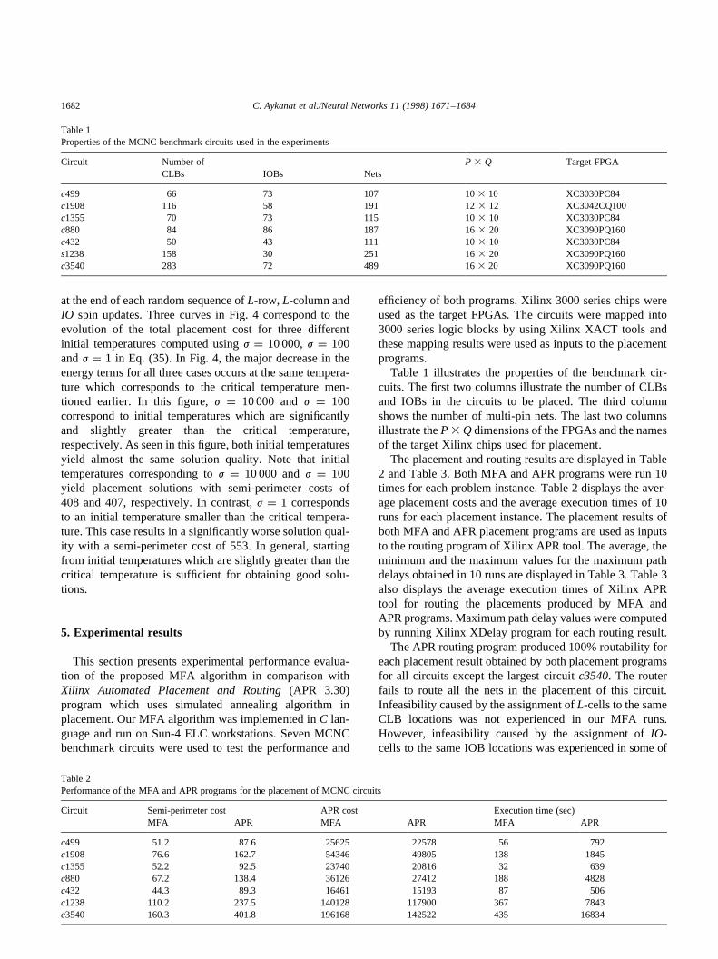
Table 1 illustrates the properties of the benchmark cir-cuits. The first two columns illustrate the number of CLBsand IOBs in the circuits to be placed. The third columnshows the number of multi-pin nets. The last two columnsillustrate theP 3 Q dimensions of the FPGAs and the namesof the target Xilinx chips used for placement.

The placement and routing results are displayed in Table2 and Table 3. Both MFA and APR programs were run 10times for each problem instance. Table 2 displays the aver-age placement costs and the average execution times of 10runs for each placement instance. The placement results ofboth MFA and APR placement programs are used as inputsto the routing program of Xilinx APR tool. The average, theminimum and the maximum values for the maximum pathdelays obtained in 10 runs are displayed in Table 3. Table 3also displays the average execution times of Xilinx APRtool for routing the placements produced by MFA andAPR programs. Maximum path delay values were computedby running Xilinx XDelay program for each routing result.

The APR routing program produced 100% routability foreach placement result obtained by both placement programsfor all circuits except the largest circuitc3540. The routerfails to route all the nets in the placement of this circuit.Infeasibility caused by the assignment ofL-cells to the sameCLB locations was not experienced in our MFA runs.However, infeasibility caused by the assignment ofIO-cells to the same IOB locations was experienced in some of

Table 1Properties of the MCNC benchmark circuits used in the experiments

Circuit Number of P 3 Q Target FPGACLBs IOBs Nets

c499 66 73 107 103 10 XC3030PC84c1908 116 58 191 123 12 XC3042CQ100c1355 70 73 115 103 10 XC3030PC84c880 84 86 187 163 20 XC3090PQ160c432 50 43 111 103 10 XC3030PC84s1238 158 30 251 163 20 XC3090PQ160c3540 283 72 489 163 20 XC3090PQ160

Table 2Performance of the MFA and APR programs for the placement of MCNC circuits

Circuit Semi-perimeter cost APR cost Execution time (sec)MFA APR MFA APR MFA APR

c499 51.2 87.6 25625 22578 56 792c1908 76.6 162.7 54346 49805 138 1845c1355 52.2 92.5 23740 20816 32 639c880 67.2 138.4 36126 27412 188 4828c432 44.3 89.3 16461 15193 87 506c1238 110.2 237.5 140128 117900 367 7843c3540 160.3 401.8 196168 142522 435 16834

1682 C. Aykanat et al./Neural Networks 11 (1998) 1671–1684

our runs. However, a single re-heating pass was sufficient forobtaining feasible solutions in all these placement instances.

The semi-perimeter cost values displayed in Table 2 cor-respond to the average normalized semi-perimeter costscomputed for the placement results of both programs asdescribed in Section 2. Here, normalization refers to assum-ing a unit square layout. That is, vertical and horizontalspans of the nets are normalized by multiplying them with1/Q and 1/P, respectively, during the computation of totalsemi-parameter cost values for Table 2. The APR costvalues correspond to the average costs computed for theplacement results of both programs according to APR’splacement cost definition. The semi-perimeter costs of theplacement results obtained by the MFA program are 105%better than those of the APR program. However, APR-costsof the placement results obtained by the APR program are16% better than those of the MFA program.

Table 4 illustrates the normalized relative performanceresults of the two placement programs. In this table, theaverages of the maximum path delay values obtained by

the Xilinx XDelay program after routing the placementresults of APR placement program are normalized withrespect to those of the MFA program. This table also illus-trates the execution times of the APR placement programnormalized with respect to those of the MFA program. Asseen in this table, the MFA placements yield slightly betterrouting results in 3 circuits out of seven circuits. APR place-ments yield 3% better routing results on the overall average.However, as seen in Tables 2 and 4, MFA placement pro-gram is significantly faster than the APR placement programin all instances. MFA placement program is 19.8 times fas-ter than the APR placement program on the overall average.Fig. 5 illustrates sample routing results of the circuitc432for placements obtained by APR and MFA.

6. Conclusions

In this paper, a fast nondeterministic cell placementalgorithm was proposed for VLSI design automation

Fig. 5. Routing results of the circuitc432for the placements obtained by (a) APR, (b) MFA.

Table 3Routing results obtained by Xilinx APR tool for placements produced by MFA and APR programs

Cicuit Maximum path delay (ns) Execution time (sec)MFA APRAvg Min Max Avg Min Max MFA APR

c499 94.9 93.0 99.6 98.5 94.8 100.4 136 85c1908 159.6 145.6 168.5 166.2 157.8 172.1 796 853c1355 94.5 92.9 98.3 91.5 84.0 93.8 98 78c880 151.2 141.1 164.6 139.1 137.2 142.6 187 266c432 173.5 162.1 192.5 178.3 174.4 185.8 202 314c1238 198.3 184.5 214.5 165.3 154.7 174.7 428 986c3540 243.5 239.6 264.4 238.5 221.9 269.5 4380 5726

1683C. Aykanat et al./Neural Networks 11 (1998) 1671–1684

based on Mean Field Annealing (MFA). The performance ofthe proposed placement algorithm was evaluated incomparison with the commercial automated circuit designsoftwareXilinx Automatic Place and Route(APR) tool forthe placement of seven MCNC benchmark circuits. Theresults show that neurocomputing approaches such as theMFA technique can be applied to practical problems andcan compete with the commercially available tools success-fully. Experimental results indicate that our algorithmachieves comparable placements with APR. However, ouralgorithm is significantly faster than APR.

Acknowledgements

This work is partially supported by the Commission of theEuropean Communities, Directorate General for Industryunder contract ITDC 204-82166, and the Turkish Scienceand Research Council under grant EEEAG-160. The authorswould like to thank Jonathan Rose for helpful discussions onFPGAs.

References

Bultan, T., & Aykanat, C. (1992). A new mapping heuristic based on meanfield annealing.Journal of Parallel and Distributed Computing, 16,292–305.

Bultan, T., & Aykanat, C. (1995). Circuit partitioning using mean fieldannealing.Neurocomputing, 8, 171–194.

Cimikowski, R., & Shope, P. (1996). A neural-network algorithm for agraph layout problem.IEEE Transactions on Neural Networks, 7 (2),341–345.

Dunlop, A. E., & Kernighan, B. W. (1985). A procedure for placement ofstandard-cell VLSI circuits.IEEE Transactions on Computer-AidedDesign, 4, 92–98.

Gislen, L., Peterson, C., & So¨derberg, B. (1992). Complex scheduling withPotts neural networks.Neural Computation, 4, 805–831.

Hokkinen, J., Lagerholm, M., Peterson, C., & So¨derberg, B. (1998). A Pottsneuron approach to communication routing.Neural Computation, 10,1587–1599.

Herault, L., & Niez, J. (1989). Neural networks and graphk-partitioning.Complex Systems, 3, 531–575.

Hopfield, J.J., & Tank, D.W. (1985). Neural computation of decisions inoptimization problems.Biological Cybernetic, 52, 141–152.

Kirkpatrick, S., Gellat, C.D., & Vecchi, M.P. (1983). Optimization bysimulated annealing.Science, 220, 671–680.

Lengauer, T. (1990).Combinatorial algorithms for integrated circuitlayout. Chichester and New York: Wiley.

Ohlsson, M., & Pi, H. (1997). A study of the mean field approach toknapsack problems.Neural Networks, 10 (2), 263–271.

Ohlsson, M., Peterson, C., & So¨derberg, B. (1993). Neural networks foroptimization problems with inequality constraints—the knapsackproblem.Neural Computation, 5 (2), 331–339.

Peterson, C., & So¨derberg, B. (1989). A new method for mappingoptimization problems onto neural networks.International Journal ofNeural Systems, 1 (3), 3–22.

Rose, J., Francis, R.J., Brown, S., & Vranesic, Z.G. (1992).Field-programmable gate arrays. Boston, MA: Kluwer Academic.

Rose, J., Elgamal, A.E., & Sangiovanni-Vincentelli, A. (1993). Architec-ture of field-programmable gate-array.Proceedings of IEEE, 81, 1013–1029.

Sechen, C. (1988).VLSI placement and global routing using simulatedannealing.Boston, MA: Kluwer Academic.

Shahookar, K., & Mazumder, P. (1991). VLSI cell placement techniques.ACM Computing Surveys, 23 (2), 142–220.

Sherwani, N. (1993).Algorithms for VLSI physical design automation.Boston, MA: Kluwer Academic.

Takahashi, Y. (1997). Mathematical improvement of the Hopfield modelfor TSP, feasible solutions by synapse dynamical systems.Neurocomputing, 15 (1), 15–43.

VandenBout, D.E., & Miller, T.K. (1989). Improving the performance ofthe Hopfield-Tank neural network through normalization and anneal-ing. Biological Cybernetics, 62, 129–139.

VandenBout, D.E., & Miller, T.K. (1990). Graph partitioning usingannealing neural networks.IEEE Transaction on Neural Networks, 1(2), 192–203.

Xilinx. (1994). The programmable gate array data book. San Jose, CA:Xilinx Inc.

Yih, J.S., & Mazumder, P. (1990). A neural network design for circuitpartitioning.IEEE Transactions on Computer-Aided Design, 9, 1265–1271.

Table 4Normalized average performance measures for the placement results obtained by MFA and APR

Circuit Maximum path delay (ns) Execution time (sec)MFA APR MFA APR

c499 1.00 1.03 1.00 14.1c1908 1.00 1.04 1.00 13.4c1355 1.00 0.96 1.00 19.9c880 1.00 0.91 1.00 25.6c432 1.00 1.03 1.00 5.8c1238 1.00 0.83 1.00 21.3s3540 1.00 0.98 1.00 38.7

Avg 1.00 0.97 1.00 19.8

1684 C. Aykanat et al./Neural Networks 11 (1998) 1671–1684