contract elements, growing conditions, and anomalous
TRANSCRIPT

Contract Elements, Growing Conditions, and Anomalous Claims Behavior in U.S. Crop Insurance
Sungkwol Park, Korean Ministry of Strategy and Finance ([email protected])
Barry K. Goodwin, North Carolina State University ([email protected])
Xiaoyong Zheng, North Carolina State University ([email protected])
Roderick M. Rejesus, North Carolina State University ([email protected])
Selected Paper prepared for presentation at the 2019 Agricultural & Applied Economics Association Annual M eeting, Atlanta, GA, July 21 – July 23
Copyright 2019 by Park, Goodwin, Zheng, and Rejesus. All rights reserved. Readers may make verbatim copies of this document for non-commercial purposes by any means, provided that this copyright notice appears on all such copies.
Contract Elements, Growing Conditions, andAnomalous Claims Behavior in U.S. Crop
Insurance
May 10, 2019
Abstract
We investigate contract elements and growing conditions associated with anomalousclaims behavior in the U.S. Federal crop insurance program. In this study, the mea-sure of “anomalous claims behavior” is based on the number of producers (in a county)placed on the “Spot Check List” (SCL) – a list generated from a government compli-ance effort that aims to detect and deter fraud, waste, and abuse in U.S. crop insurance.Using county-level data and various econometric approaches that control for featuresof this data set (e.g., count nature of the dependent variable, censoring, and potentialendogeneity), we find that the following crop insurance contract attributes influencethe extent of anomalous claims behavior in a county: (a) the ability to insure smallerfields through “optional units”, (b) the coverage level choice, and (c) the total numberof acres insured. In addition, our empirical analysis suggest that anomalous claims be-havior statistically increases when extreme weather events occur (e.g., droughts, floods)and when economic conditions are unfavorable (i.e., high input costs that lower profitlevels). Results from this study have important implications for addressing potentialunderwriting vulnerabilities in crop insurance contracts, and the frequency of morerigorous compliance inspections.
Keywords: Spot Check List; Insurance fraud; Crop Insurance; Simulated MaximumLikelihood Estimation; Control function approach
JEL Classification Numbers: Q14; Q18; G22
1
1 Introduction
The Risk Management Agency (RMA) of the U.S. Department of Agriculture (USDA) is
the government agency in charge of administering the US crop insurance program. As part
of its efforts to detect and deter fraud, waste, and abuse in the Federal crop insurance pro-
gram, the RMA developed and implemented the so-called “Spot Check List” (SCL) program
in 2001(USDA-RMA, 2006). Under this SCL effort, the RMA and their partners utilize
complex and proprietary algorithms to analyze their massive data warehouse that contains
extensive crop insurance contract data, as well as information from other related databases
(e.g. weather data and/or other administrative data from other USDA agencies). The aim
of the SCL process is to detect individual producers whose claims behavior demonstrate
atypical patterns indicative of potential fraud, waste, and abuse.
One of the main outputs from this process is the SCL itself – an annual list of insured
farmers, identified based on objective and data-driven statistical techniques, whose loss ex-
periences are considered “anomalous” relative to similar producers in the same geographic
area (i.e., typically within a county), producing the same crop and using the same cropping
practices. Therefore, the number of SCL producers in a county can be regarded as a measure
of “anomalous claims behavior” suggestive of the extent of crop insurance fraud, waste, and
abuse in that county.1 Everything else being equal, larger numbers of SCL producers (in
a county) potentially indicate that there are likely more fraudulent claims or more claims
misrepresentation in that county.
The objective of this study is to examine crop insurance contract elements and growing
conditions that likely influence the degree of anomalous claims behavior in a county. We
first examine whether the underwriting design of the crop insurance contract itself is a
contributing factor, since opportunistic abuses and misrepresentations can be prompted by
1As mentioned in USDA-RMA (2018), being included on the SCL does not indicate that a producerhas explicitly engaged in fraud. Rather, it implies that the claim behavior of a producer on the SCL is notconsistent with those of other similar producers in the same geographic area and warrants more extensiveinvestigation.
2

flexible insurance options and provisions. We focus on the unit structure, coverage level, and
type of insurance chosen by the insured farmers. The unit structure defines how acres are
insured.2 Indeed, Knight and Coble (1999) found that the loss cost ratios3 tend to be higher
for optional units than those for basic units. Considering that producers can choose their
coverage level between 50% and 85% (in 5% increments) under the buy-up coverage option in
US crop insurance, we also examine whether higher coverage levels lead to more anomalous
claims behavior.4 Walters, Shumway, Chouinard and Wandschneider (2015) found evidence
that producers obtained excess returns by selecting optional units and buy-up coverage.
Lastly, producers can choose between yield-based and revenue-based policies. Revenue-based
policies insure against losses due to both low crop yields and price declines, while yield-based
policies offer protection against low yields only. We consider whether less exposure to price
risk under the revenue-based policies contributes to a decrease in anomalous claims behavior.
It is also possible for more revenue-based policies to lead to more anomalous claims behavior,
as revenue-based polices are more costly than yield-based ones.
In addition to crop insurance contract characteristics, we also examine the roles of two ad-
ditional categories of variables in determining anomalous claims behavior. First, unfavorable
economic or profit conditions in a particular year may be another motivating factor for pro-
ducers to commit insurance claims fraud, waste, and abuse. For this, we use a county-level
net income variable (the difference between income and expenses) as a measure of produc-
ers’ profits (and the general economic environment). Also, anomalous claims behavior can
be triggered by extreme weather conditions. Given the fact that not all claims are audited,
2Under the current federal crop insurance program, producers have four options: optional, basic, enter-prise, and whole-farm units. Under the optional unit, each field and crop can be insured separately whileunder other options, several units are combined. Specifically, basic units combine all of the owned and cashrented acres in the same county by the same producer, but share-leased units or units of a different cropcannot be combined. Enterprise units combine all acreage of the same crop by the insured in a countyinto one unit. In other words, share-leased acres can be combined with owned and cash rented acres inone enterprise unit. Whole-farm units combine all crops by the insured in the same county. All four unitstructures are illustrated in section 2.1 with an example.
3Loss cost ratio is the ratio of indemnities to liabilities.4Producers can purchase the minimum catastrophic coverage (CAT) that will protect up to 50% of their
expected yield/revenue, if a loss occurs. Producers can buy-up to higher levels of coverage with the optionto insure up to 85% of the expected yield/revenue.
3

when severe drought or extremely wet conditions (e.g., floods) occur, producers may be more
likely to engage in fraudulent activities because the extreme weather conditions make it more
difficult to distinguish between fraudulent claims and legitimate ones. For this reason, we
include a rich set of weather variables in our empirical analysis.
Empirically estimating the effects of crop insurance contract elements and growing con-
ditions on the extent of county-level anomalous claims behavior is challenging for a number
of reasons. First, the data available to us has three important features (and limitations)
that need to be taken into account in the estimation: (1) our dataset is at the county-level
with a panel (or longitudinal) structure, (2) our dependent variable, the number of SCL
producers in a county, is a count variable, and (3) our dependent variable is left censored
due to government regulations on data confidentiality when reporting SCL data. To accom-
modate the three data features described, we estimate a random effects count model with
censoring, using the simulated maximum likelihood approach.5 Another important feature
of the data set (and the variables included in the specification) is that several explanatory
variables in our regression models are potentially endogenous. Therefore, we also employ
the control function approach (Hausman, 1978; Wooldridge, 1997, 2014; Terza, Basu, and
Rathouz, 2008) to correct for possible bias due to endogeneity.
Our results provide strong evidence that county-level variables associated with character-
istics of the crop insurance contracts producers purchase are strong predictors of anomalous
claims behavior. For instance, a larger proportion of acres insured as optional units is associ-
ated with more anomalous claims behavior. Higher average coverage levels (in a county) and
larger number of insured acres are also strongly linked with increased incidence of anomalous
claims behavior. In addition, our empirical analysis also indicate that unfavorable economic
and weather conditions strongly influence the extent of anomalous claims behavior in a
county. The crop insurance contract elements associated with anomalous claims behavior
5Although this is our “preferred” estimation procedure (since it accounts for all three data featuresabove) we also utilized fixed effects linear models and fixed effects count models that accounts for some (butnot all) of the data features described above.
4

are potential underwriting vulnerabilities that RMA needs to address to further discourage
fraud, waste, and abuse in the system. Further study is required to determine the appro-
priate underwriting or premium-rating adjustments needed to curb the anomalous claims
behavior linked to these “vulnerable” contract elements. On the other hand, our empirical
results regarding insureds potentially taking advantage of unfavorable economic and weather
conditions to undertake fraud, waste, or abuse, indicate that fraud auditing standards and
compliance inspection efforts may need to be tightened in times of adverse economic and
weather conditions affecting the agricultural economy.
The remainder of this paper is organized as follows. The next section introduces the SCL
program and the unit structure in US federal crop insurance. In section 3, we describe the
data and variables used in our empirical analyses. In section 4, we discuss the econometric
model developed to account for the special features of our data. In section 5, the main
findings from our estimations are discussed. Concluding comments and policy implications
are provided in the final section.
2 Background
Objective and data-driven statistical techniques are employed to annually develop the list of
SCL producers whose loss experience is considered “anomalous” relative to similar producers
in the same geographic area (typically within a county), producing the same crop and using
the same cropping practices. To develop the SCL, previous research and “on-the-ground”
observations gathered by RMA field staff and partner insurance companies (called Approved
Insurance Providers (AIPs)) are first utilized to identify different “scenarios” that are sugges-
tive of potential fraud, waste, or abuse. For example, one scenario-based detection algorithm
may pertain to finding those producers that have large multi-year losses that are consistently
higher than their peers in the same county. Another algorithm may aim to detect behavior
consistent with known fraud schemes that have previously been recognized.
5
All producers flagged by these detection procedures are then used to create a pool of
producers to be included in the SCL. The SCL developed for producers of spring-planted
crops (e.g. corn, soybeans) that are based on data analyzed through a particular crop year
(say, in 2017, where data through December 2017 is analyzed) is typically finalized no later
than the first quarter of the following year (i.e., no later than April 1, 2018). The finalized
SCL is then forwarded to the local USDA Farm Service Agency (FSA) county offices where
the SCL farmers are located, and to the AIPs whose clients are included in the list. Soon
after, the AIPs send a formal written letter to their clients on the list informing them of
their inclusion, and that their operations are subject to inspection and/or review during the
growing season. The FSA county offices and/or the AIPs then conduct infield inspections
and/or policy reviews of the SCL producers, although typically not all SCL farmers are
inspected/reviewed due to time and resource constraints.6
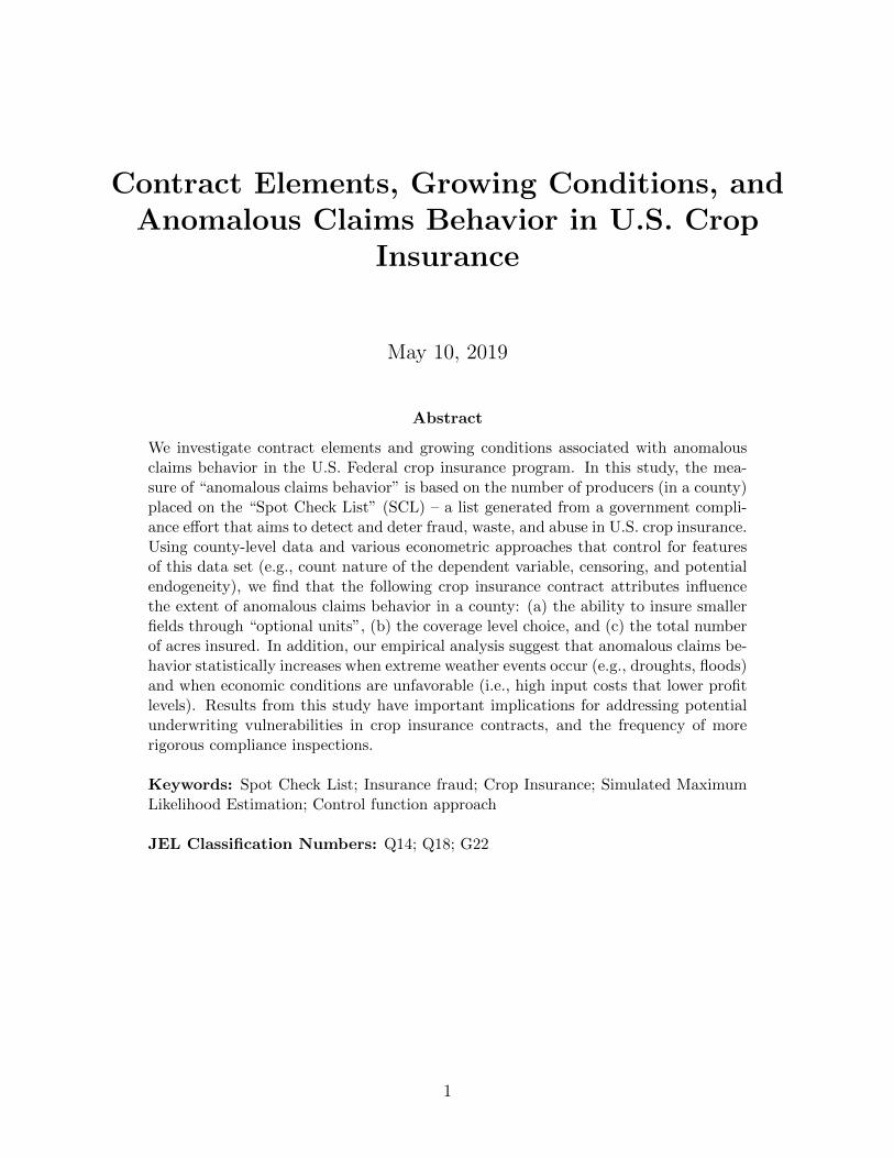
2.1 Unit Structure
Since unit structure is one of the main contract element we examine in this study and many
readers may not be familiar with it, here we provide detailed definitions of the different
unit structure options available in the US federal crop insurance program using an example.
Suppose a producer has cropland units in a county shown in Figure 1. The producer has six
units, identified with letters A through F. The fields for corn are from A to C and those for
soybeans are from D to F. In addition, since unit choices are based on ownership structure
as well as the geographic location, we need to know whether each field is owned, cash-rented,
or share-rented by the producer. Assume that the producer owns fields A and D, rents fields
B and E on a cash basis, and has a crop share arrangement on fields C and F.
6Note that from 2001 to 2011 the FSA had sole responsibility for conducting infield inspections of allSCL producers (i.e., both growing season and pre-harvest inspections) to assess whether the condition ofthe insured crop is consistent with other non-SCL producers in the area. Beginning in 2012, AIPs assumedresponsibility for inspecting a subset of producers on the SCL, with the FSA still responsible for the remainingproducers. The AIP inspection is more comprehensive than the FSA in the sense that they perform bothinfield inspections and a full policy review. For a more detailed description of what is involved in an AIPinspection and full policy review, see: https://www.rma.usda.gov/pubs/ra/sraarchives/19sra.pdf.
6

In this example, the producer could choose to insure his/her fields with six optional units
if field-specific production records are available and the boundaries of the units are readily
discernible (i.e., three for corn and three for soybeans). An insurance guarantee is assigned to
each optional unit and each unit would stand alone when determining indemnities. However,
the optional units are not eligible for a premium discount.
The farmer could also choose to insure his/her fields with three other unit structures. A
basic unit7 consists of all croplands of a single crop that are either owned or cash rented.
In the case of a single crop share arrangement, a separate basic unit is available. Thus, the
producer in our example can have two basic units of corn and two basic units of soybeans
(i.e., a total of four basic units). The first corn basic unit consists of fields A and B. The other
basic unit consists of field C. The first soybean basic unit consists of fields D and E. The
second basic unit consists of field F. Each basic unit has its own insurance guarantee. The
move to basic units from optional units may decrease the frequency with which indemnities
are received. Because of this potential decrease in indemnities, insurance premiums are lower
for basic units than for optional units.8
An enterprise unit consists of all acreage of the same crop in the county. Therefore, our
producer could form two enterprise units: one for corn and one for soybeans. The expected
indemnities are lower under enterprise units than under basic units because the losses from
owned or cash rented units may be made up by gains on the share rented units. Enterprise
insurance premiums are lower than those of basic units to reflect the lower magnitude of
loss.
A whole-farm unit consists of all croplands in the same county being placed into a single
insurance unit. Thus, the farm in our example could insure all acres of cropland together,
that is, the corn and soybeans fields would be insured together in one whole-farm unit.9
7The insured automatically qualifies for basic units without exception (2015 Crop Insurance Handbook).8Since 1988, producers have received a fixed 10% discount on their premiums if they do not insure
optional units.9For more information on unit structure, see Babcock and Hart (2005), which offer a detailed explanation
that includes a calculation of liabilities and indemnities for each unit choice.
7

3 Data
We obtained county-level “Spot Check List” (SCL) data from USDA-RMA over the 2001-
2015 time period through a Freedom of Information Act (FOIA) request and special agree-
ment. Because data on county-level unit structure, a key contract element examined in this
study, are only available from 2002,10 our regression analysis only utilizes data from 2002
to 2015. The SCL data cover insured producers of the four major row crops (corn, soy-
beans, wheat, and cotton), in addition to tobacco. Also, only yield-based and revenue-based
individual policies are considered.11 As a result, our data account for 69.59 % of all crop
insurance policies for which acreage had been reported to USDA-RMA between 2002 and
2015. These data come from 2,162 counties across all U.S. states, except Alaska, Hawaii,
and Rhode Island.12
More importantly, due to government regulations regarding data confidentiality, the num-
ber of SCL producers in a county is only reported in our data set if the county had at least
four producers on the SCL in that year. We therefore cannot exactly identify the number
of producers on the SCL in a county for a particular year when the number of producers on
the SCL was less than four. Our empirical specification below is designed to accommodate
this important data feature. The numbers of counties with more than three SCL producers
from 2001 to 2015 are presented in Table 1. The numbers ranged from 124 to 308 during the
sample period. On average, 235 counties had at least four SCL producers in a particular year
and these counties had approximately seven SCL producers every year. Table 2 summarizes
the detailed frequency distribution of counties with each number of SCL producers by year.
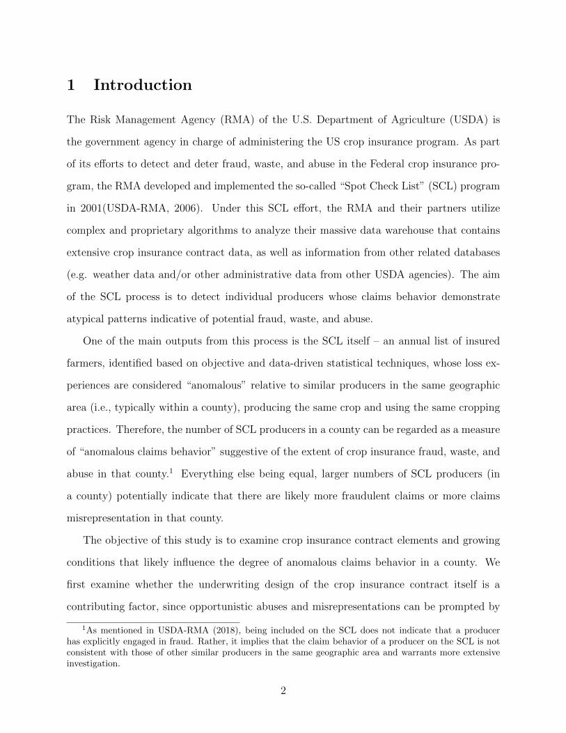
Figure 2 provides the spatial distribution of the total number of SCL producers from 2001
to 2015.13 We note that counties with substantial SCL producers are scattered throughout
10See: https://www.rma.usda.gov/data/sob/scc/index.html.11Other “less-popular” plans like the Area Risk Protection Insurance (ARPI) and Whole Farm Revenue
Protection (WFRP) Insurance policies are not considered in this study.12Crop insurance policies from 2002 to 2015 were sold in 2,831 counties across all 50 U.S. states.13Given the limitation on the number of SCL producers reported in our data, if the number of SCL
producers in a year was less than four for a county, then the number of SCL producers in this figure was
8

the continental U.S. with some clustering in the upper Midwest, the Dakotas, the Plains
(i.e., Kansas, Nebraska and the Texas Panhandle), and the Southeastern States (i.e., North
Carolina, South Carolina, Georgia, and Florida).
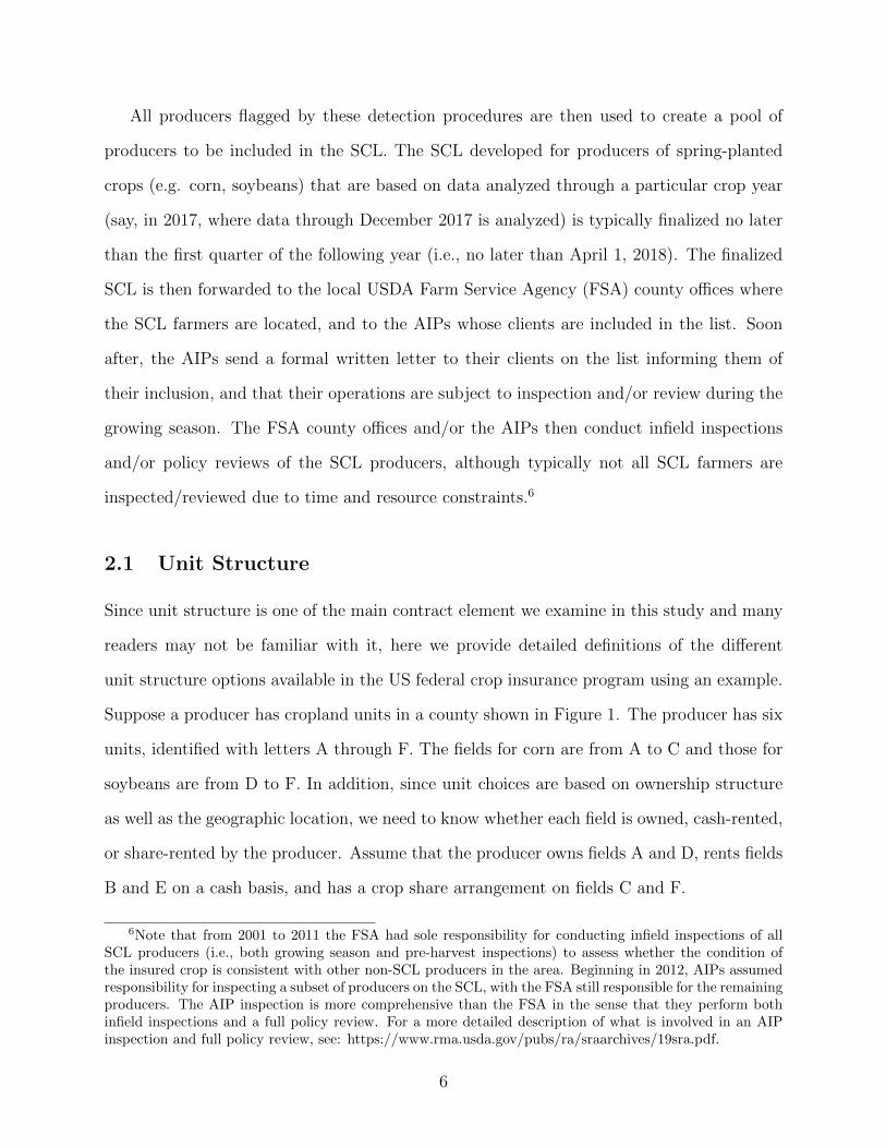
Figure 3 and 4 provide the spatial distributions of the number of SCL producers for
selected years between 2001 and 2015. When the SCL program started in 2001, the Dakotas
and the Plains had larger numbers of SCL producers, but the clusterings gradually disap-
peared during the 10-year period from 2001 to 2010 (as seen in Figure 3). Figure 4 presents
the spatial distributions of the number of SCL producers from 2012 to 2015. It appears
that for these four years, a number of SCL producers were in Iowa, Missouri, Illinois, and
Kansas.14
We constructed a number of county-level variables to represent contract elements and
growing conditions that could potentially influence anomalous claims behavior. First, for
factors related to crop insurance contract design, we use the county-level crop insurance ex-
perience data publicly available from USDA-RMA. As discussed in the introductory section,
we focus on unit structure, coverage level, and insurance type. To examine whether the
ability to separately insure smaller fields through optional units influence the potential risk
of fraud, waste, and abuse, we use the county-level percentage of acres insured as optional
units as our main county-level variable. Figure 5 shows the percentages of acres insured
under the four different types of units from 2002 to 2015, and Figure 6 presents the percent-
ages of acres insured as optional units by crop over time. In 2002, on average, 57% of the
acres insured were contracted as optional units and then this percentage increased to 62%
in 2008. However, it decreased considerably between 2008 and 2015, partly because the gov-
ernment raised the premium subsidies for the use of enterprise units by a significant amount
in 2009 (the effect can be clearly seen in Figure 5), and in 2015, only 32% of the acres were
coded as zero.14It is important to emphasize here that the SCL procedure is national in scope. Even with these
geographical SCL “clusterings” observed over time, there was no explicit attempt to “target” a specificregion in the US or a particular set of crops. These SCL “clusterings” over time are simply a result ofobjective and data-driven algorithms applied nationally in order to detect anomalous behavior.
9
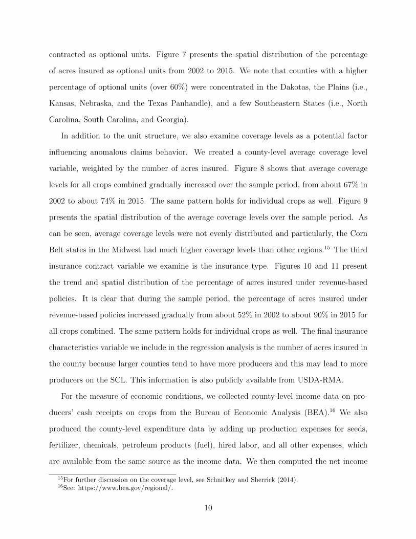
contracted as optional units. Figure 7 presents the spatial distribution of the percentage
of acres insured as optional units from 2002 to 2015. We note that counties with a higher
percentage of optional units (over 60%) were concentrated in the Dakotas, the Plains (i.e.,
Kansas, Nebraska, and the Texas Panhandle), and a few Southeastern States (i.e., North
Carolina, South Carolina, and Georgia).
In addition to the unit structure, we also examine coverage levels as a potential factor
influencing anomalous claims behavior. We created a county-level average coverage level
variable, weighted by the number of acres insured. Figure 8 shows that average coverage
levels for all crops combined gradually increased over the sample period, from about 67% in
2002 to about 74% in 2015. The same pattern holds for individual crops as well. Figure 9
presents the spatial distribution of the average coverage levels over the sample period. As
can be seen, average coverage levels were not evenly distributed and particularly, the Corn
Belt states in the Midwest had much higher coverage levels than other regions.15 The third
insurance contract variable we examine is the insurance type. Figures 10 and 11 present
the trend and spatial distribution of the percentage of acres insured under revenue-based
policies. It is clear that during the sample period, the percentage of acres insured under
revenue-based policies increased gradually from about 52% in 2002 to about 90% in 2015 for
all crops combined. The same pattern holds for individual crops as well. The final insurance
characteristics variable we include in the regression analysis is the number of acres insured in
the county because larger counties tend to have more producers and this may lead to more
producers on the SCL. This information is also publicly available from USDA-RMA.
For the measure of economic conditions, we collected county-level income data on pro-
ducers’ cash receipts on crops from the Bureau of Economic Analysis (BEA).16 We also
produced the county-level expenditure data by adding up production expenses for seeds,
fertilizer, chemicals, petroleum products (fuel), hired labor, and all other expenses, which
are available from the same source as the income data. We then computed the net income
15For further discussion on the coverage level, see Schnitkey and Sherrick (2014).16See: https://www.bea.gov/regional/.
10

as the difference between income and expenditure.
Lastly, we created a rich set of weather variables to be included in the specification (and
are used to examine whether adverse weather conditions affect anomalous claims behavior).
First, we created several variables that represent yearly weather disasters, averaged from
monthly extreme heat, extreme drought, and extreme wet conditions. For the measure
of extreme heat conditions, we use county-level total degree days above 30 ◦C during the
months of June-September using the method of Schlenker and Roberts (2006).17 For extreme
drought and extreme wet conditions (e.g. flood), we collected the monthly Palmer Drought
Severity Index18 from April to October at the state-level from the National Oceanic and
Atmospheric Administration (NOAA) and constructed two variables, one for dryness and
the other for wetness. In addition, we also collected monthly county-level data on average
precipitation (mm), minimum temperature (◦C), and maximum temperature (◦C) for the
growing months (from April to October), based on the work of Schlenker and Roberts (2009)
and available data from PRISM.19 Table 3 lists all the variables used in our estimation and
the corresponding data sources. Summary statistics are displayed in Table 4.
4 Estimation
There are three main features of our dataset. First, our data is a panel dataset at the county
level. Second, the dependent variable, the number of producers on the SCL in each county,
is a count variable. Third, the dependent variable is left censored, that is, it takes the value
of zero when the number of producers on the SCL is less than 4 (i.e., we only know that the
number can be 0, 1, 2, or 3). We estimate three empirical models. Each model has its own
advantages and disadvantages.
17For a detailed derivation and further discussion, see Schlenker and Roberts (2006) and SI Appendix ofSchlenker and Roberts (2009).
18To identify the abnormality of a drought in a region for a particular month, short-term drought index(i.e., the Palmer Z index) is used. It indicates that the Z-index represents monthly drought conditions withno memory to previous monthly moisture deficits or surpluses.
19See http://www.prism.oregonstate.edu. Further note that the “average” values here were averagedacross the days in a mont and across different weather stations in a county.
11

Formally, let yit denote the number of producers on the SCL in county i and year t (i.e.,
SCLit). First, we estimate the following fixed effects linear model,
yit = X′
itΘ + αi + εit, (1)
where Xit is a vector of explanatory variables including the year fixed effects. The term αi is
the county fixed effect to control for the time-invariant county level unobserved heterogeneity.
For example, similar claim filing practices may be common in a county since producers’
attitudes can be influenced by their peers and neighbors within the same county.20 Finally,
εit denotes an idiosyncratic error term. The linear model does not take into account the count
data generating process and the fact that the dependent variable is left censored. However,
it requires the least assumptions among the three models we estimate.
The second model we estimate is the fixed effects Poisson model, which accommodates
the first two features of our data discussed above. More specifically, in this model, we assume
yit follows the Poisson probability density distribution,
f(yit|λit, αi) =exp(−αiλit) · (αiλit)
yit
yit!,
where λit = exp(X′itΘ). A nice feature of the Poisson model is that Wooldridge (1999) shows
that estimates from the Poisson maximum likelihood estimation (MLE) are consistent as
long as the conditional expectation assumption E(yit|Xit, αi) = αi exp(X′itΘ) holds. As a
result, the fixed effects Poisson model requires much less assumptions than it seems. In
contrast, another popular count data model, the fixed effects negative binomial (NB) model
(Hausman, Hall, and Griliches, 1984), requires the full distributional assumption for the
estimates to be consistent.
Finally, to accommodate all three data features at the same time, we employ the random
effects Poisson model with censoring. In this model, the probability function for the observed
20e.g., An “every one does it” attitude may result in a higher potential risk of fraud, waste, and abuse.
12
dependent variable yit (i.e., the censored number of producers on the SCL) is
Pr(yit|Xit; Θ, αi) =
f(y∗it = 0, 1, · · · , or L|Xit; Θ, αi) if yit ≤ L,
f(y∗it = yit|Xit; Θ, αi) if yit > L,(2)
where y∗it is the latent dependent variable (i.e., the true number of producers on the SCL)
left censored at L. In this case,
Pr(yit ≤ L|Xit; Θ, αi) = f(0|Xit; Θ, αi)+f(1|Xit; Θ, αi)+· · ·+f(L|Xit; Θ, αi) = g(L|Xit; Θ, αi).
Therefore, assuming the independence between observations conditional on covariates and
unobserved heterogeneity, the likelihood function for all observations from county i is
Pr(yi1, ..., yiTi|Xi1, ..., XiTi
; Θ, αi) =
Ti∏t=1
f(yit|Xit,Θ, αi)dit · g(L|Xit; Θ, αi)
(1−dit)
=
Ti∏t=1
[exp(−αiλit)(αiλit)
yit
yit!
]dit· g(L|Xit; Θ, αi)
(1−dit),
where dit = 1 if yit > L, dit = 0, otherwise.
Assuming that the unobserved heterogeneity αi follows a distribution h(αi), we can fur-
ther derive the likelihood function conditional only on the observed covariates as,
Pr(yi1, ..., yiTi|Xi1, ..., XiTi
; Θ)
=
∫ Ti∏t=1
[exp(−αiλit)(αiλit)
yit
yit!
]dit· g(L|Xit; Θ, αi)
(1−dit)h(αi) dαi.(3)
In order to approximate the integral in (3), we further assume that the unobserved het-
erogeneity αi follows a log-normal distribution with log mean µ and log variance σ2 (i.e.,
αmi = exp(µ + σumi )) and draws umi , m = 1, 2, · · · ,M randomly from a standard normal
distribution based on Halton sequences.21 Then we maximize the following log-likelihood
21For further discussion on Halton draws, see Cappellari and Jenkins (2003), Haan and Uhlendorff (2006),
13
function,
N∑i=1
log
{1
M
M∑m=1
Ti∏t=1
[exp(−αm
i λit)(αmi λit)
yit
yit!
]dit· g(L|Xit; Θ, αm
i )(1−dit)
}
where N is the number of counties in our dataset.
4.1 Endogeneity
The second challenge we face in our empirical analysis is that several of the explanatory
variables are potentially endogenous. First, the county-level percentage of acres insured as
optional units is likely to be endogenous since there may exist unobservable latent variables
that influence both this variable and the dependent variable yit (i.e., the number producers
on the SCL). For example, if on-site inspections were heavily enforced in the preceding year,
but differently among acres insured under unit structures (e.g. focused on acres insured
as optional units), then in the current year, producers may be less likely to insure acres
as optional units and the number of producers on the SCL can also be affected. Similarly,
average coverage level, percentage of acres insured under revenue-based policies, and number
of acres insured are also likely to be endogenous as they are all decision variables by the
producers. In addition, the net income variable depends on farmers’ decisions for input
expenditure and hence is also potentially endogenous.
To correct for the potential bias caused by endogeneity, for the linear panel data fixed
effects model, we use the two-stage least squares (2SLS) estimator. For the other two non-
linear models, we employ the control function approach (Hausman, 1978; Wooldridge, 1997,
2014; Terza, Basu, and Rathouz, 2008). More specifically, the first stage of the control
function approach is the same as that of 2SLS where each endogenous variable is regressed
on the exogenous variables in the model as well as a set of instrumental variables. After
estimation, the residual is retained. In the second stage of the control function approach,
and Train (2003).
14

the residuals from all first stage regressions for the endogenous variables are included in
the main regression as additional explanatory variables. Terza, Basu, and Rathouz (2008)
show that in a non-linear framework, the control function estimator is consistent, while the
nonlinear 2SLS approach is not. The intuition of the control function approach is it divides
the variation in each endogenous variable into two parts. The first one is the portion of
the variation explained by the set of exogenous and instrumental variables. The second one
is the remaining variation and source of endogeneity. By including the residual from the
first stage regression in the main model, the remaining variation in the endogenous variable
can be regarded as exogenous. Also, the standard errors for the second-stage estimation are
obtained using the bootstrapping procedure.22
To implement the control function approach, we created several instrumental variables.
USDA-RMA’s publicly available county-level crop insurance experience data (i.e., the Sum-
mary of Business) report the amounts of subsidized premiums for policies with different
characteristics. We divide all the policies in the data into eight groups along the following
three dimensions: optional versus non-optional units, low (below 70%) versus high (from
70% to 85%) coverage levels, and revenue-based versus yield based policies. We then created
eight per acre subsidy variables for the eight groups, one for each group. But in estimation
below, we only use six (first-lagged) variables because two combinations (the combination of
optional units, low coverage level coverage, and revenue-based policies and the combination
of optional units, high coverage level, and yield-based policies) have relatively smaller num-
ber of observations and using them would result in a significant loss of of observations. Due
partly to the fact that insurance premiums in a county are determined by producers’ liabil-
ities in the county and the loss cost ratio (i.e., indemnities/liabilities) history of the county
and then the subsidy amounts are percentages of the premiums, there are both temporal and
county-level variations in the per-acre subsidy variables.23 Table 5 presents the summary
22For details about bootstrapping in the two-stage regression with instrumental variables, see Guan (2003).23The subsidy rate, which is the ratio of subsidy to liabilities, also depends on the coverage levels and
types of insurance plans producers choose.
15

statistics for the per acre subsidy variables. The amounts of subsidies for different kinds
of policies influence which type of policies producers purchase and hence the county-level
percentage of acres insured as optional units, the average coverage level and percentage of
acres insured under revenue rather than yield based policies. Also, the overall increase and
decrease of the subsidies affect how many acres are insured. On the other hand, it is unlikely
for the subsidies to have a direct effect on the number of producers on the SCL.
The second set of instruments we use is the lagged weather variables. When farmers
choose insurance policies and make decisions on inputs in the current year, their decisions
may be influenced by their experiences in the previous year, especially the weather conditions.
On the other hand, it is unlikely that weather conditions last year would affect producers’
claims filing behavior and hence the number of producers on the SCL this year.
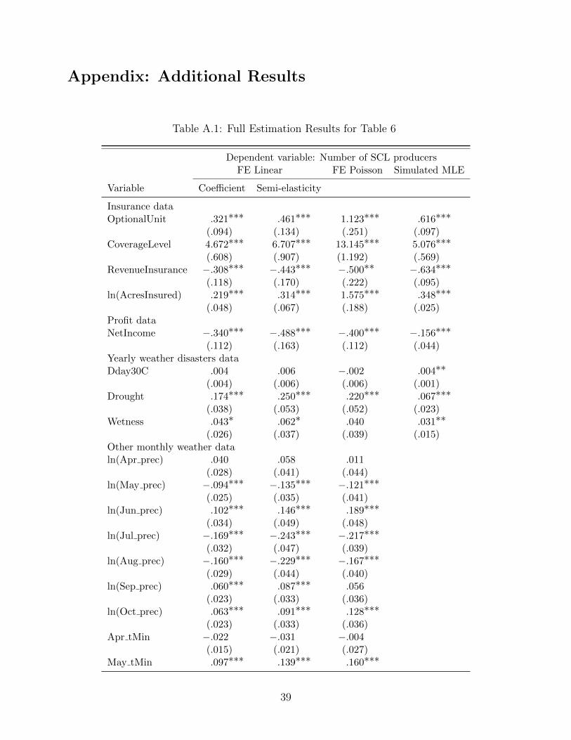
5 Results
We first estimated the three econometric models assuming all explanatory variables are ex-
ogenous. The coefficient estimates are reported in Table 6. The regressions for the fixed
effects linear and Poisson models include all variables listed in Table 4 and the year dum-
mies, but the coefficients for the monthly precipitation and temperature variables and year
dummies are omitted for brevity. On the other hand, the regression for simulated maxi-
mum likelihood estimation (MLE) does not include monthly precipitation and temperature
variables and year dummies to avoid computational difficulties, but yearly extreme heat,
drought and wetness condition variables are still included. The full results are reported in
Table A.1 in the appendix. Furthermore, to make the results from the three models compa-
rable with one another, using the estimates, we further computed the semi-elasticity of the
dependent variable with respect to each explanatory variable, that is,∂ lnE(yit|·)
∂xitwhere xit
is one explanatory variable. For the linear fixed effects model, the semi-elasticities and the
coefficient estimates are different, while the two are the same for the other two models. All
16

the results are reported in Table 6. The semi-elasticity has the interpretation as the effect
of one unit increase in xit on the percentage change in E (yit).
As we can see from the table, in general, the results are robust across different models
in terms of the signs and statistical significances of the coefficient estimates. However, the
magnitudes of the estimates do differ somewhat across different models. As the simulated
ML estimator takes into account all three of the main features of our dataset, below we
focus our discussion on results from this model. First, 1% increase in the percentage of acres
insured as optional units increases the number of producers on the SCL by 0.62%. Second,
when the average coverage level in a county increases by 1%, the number of producers on the
SCL in the county will increase by 5.08%. Third, the percentage of acres insured under the
revenue based rather than yield based policies is estimated to have a negative and statistically
significant effect on the number of producers on the SCL. This finding is different from the
study of Walters, Shumway, Chouinard, and Wandschneider (2015), who argue that the
decision to purchase revenue-based policies did not lead to opportunistic behaviors. Fourth,
1% increase in the number of acres insured increases the number of producers on the SCL by
0.35%. This result implies that the incidence of anomalous claims behavior increases with
the number of acres insured.
With regards to other factors, our results show that net income has a negative effect on
anomalous claims behavior. When the net income for the county increases by $100 million,
the number of producers on the SCL decreases by 15.6%. Our results also reveal that weather
disasters in a particular period increase anomalous claims behavior. Specifically, the more
severe or extreme weather producers encounter during the months of April-October, the
higher the number of producers on the SCL. For example, when monthly average number
of degrees days above 30 ◦C between June and September increases by one, the number of
producers on the SCL will increase by 0.4%. In the case of drought, when monthly averaged
drought level between April and October increases by one, the number of producers on the
SCL will increase by 6.7%. They are all statistically significant at the 1% or 5% level. These
17

findings provide strong evidence that unfavorable weather conditions lead to more anomalous
claims behavior. Insured producers seem to be taking advantage of these adverse weather
conditions as the backdrop to submit anomalous claims (since it is harder for non-legitimate
claims to be recognized in this situation).
5.1 Correcting for Endogeneity
We then re-estimated the three models above using the 2SLS or the control function approach
to correct for the possible bias from the potentially endogenous variables. In the first stage
of the 2SLS or the control function approach, each endogenous variable is regressed on the
instrumental variables (the six lagged subsidy variables and lagged weather variables in
our context) and the exogenous variables in our main model. Results from the first stage
regressions are collected in Table A.2 in the appendix. As we can see from the table, by and
large, the instrumental variables appear to be associated with the potentially endogenous
variables with the expected signs and they are statistically significant. For example, higher
per acre subsidy for the optional units leads to an increase in the percentage of acres insured
as optional units. On the contrary, per acre subsidy for the non-optional units shows the
opposite effect on the percentage of acres insured as optional units. Table A.2 also reports
the F statistics for the null hypothesis that the coefficients of the instrumental variables are
equal to zero. All of these first-stage F statistics have very small p-value and reject the null
hypothesis that our instrumental variables are weak.
Results from the second-stage of the control function approach are reported in Table 7
with the associated semi-elasticities for the fixed effects linear model.24 Again, the results
are robust across different models in terms of the signs and statistical significance of the coef-
ficient estimates. Therefore, we again focus our discussion on the results from the simulated
ML estimator reported in Table 7. Compared with the results in Table 6, we note that our
main results are robust with respect to whether endogeneity is controlled for or not, in terms
24The full results for Table 7 are reported in Table A.3 in the appendix.
18

of the signs and statistical significance of the coefficient estimates. The magnitudes, however,
are generally larger when potential endogeneity is controlled, as compared to when potential
endogeneity is ignored, except for the case of the optional unit variable (i.e., although the
magnitude of the optional unit coefficient is fairly similar in both estimations). For example,
1% increase in the average coverage level and the number of acres insured, increases the
number of producers on the SCL by 6.05% and 0.41%, respectively. A 1% increase in the
proportion of optional unit acres also increase the number of SCL producers in the county by
about 5%. On the other hand, 1% increase in the percentage of acres insured with revenue-
based policies (rather than yield based policies), decrease the number of producers on the
SCL by 1.30%. In addition, the results in Table 7 show a much larger effect of county-level
net income on anomalous claims behavior. It is estimated that when the net income for the
county increases by $100 million, the number of producers on the SCL decreases by 20.3%.
These results show that it is important to correct for bias from potential endogeneity, when
estimating the effects of insurance contract variables on anomalous claims behavior. Fi-
nally, with regards to the effects of adverse weather, our results from Table 7 again show
that weather disasters in a particular period do increase anomalous claims behavior, and
the results are similar to those from Table 6, in terms of signs, statistical significance and
magnitudes.
6 Conclusions
This study empirically examines whether certain crop insurance contract elements and grow-
ing conditions influence the occurrence of anomalous claims behavior in the U.S. crop insur-
ance program. “Anomalous claims behavior” is measured here using the number of producers
included in the SCL for a county. These SCL producers are identified based on claims be-
havior that is not consistent with other producers in a county, producing the same crop and
using the same practices (i.e., hence they are deemed “anomalous”). County-level variables
19

representing contract elements and growing conditions are then merged together with the
SCL data to construct a county-level panel data set that is used to achieve the study ob-
jective. Several econometric procedures are then implemented to accomodate several unique
features of this county-level data set (e.g., the count nature and censoring in the dependent
SCL variable, and potential endogeneity of the independent variables), which consquently
allows one to have more precise parameter estimates.
Our results provide strong evidence that several contract components producers choose
strongly affects the extent of anomalous claims behavior in a county. For instance, as the
percentage of acres insured as optional units increase, the number of SCL producers in a
county also increase. Our analysis also show that average county-level coverage levels, pro-
portion of revenue-based policies, and total number of insured acres in a county are also
positively related to the number or SCL producers (and consequently the degree of anoma-
lous claims behavior in a county). These contract elements strongly related to anomalous
claims behavior provides indication of potential underwriting vulnerabilities that may merit
further investigation and study. The adverse claims behavior likely due to optional unit
choice suggest that the premium “surcharge” for insuring optional units may not be ad-
equate. An updated analysis akin to the approach in Knight et al. (2010) is needed, but
utilizing more recent data that accounts for the higher enterprise unit subsidies implemented
in the 2008 Farm Bill. Re-examining the coverage level relativities used in establishing pre-
miums for yield- and revenue-based policies may also be appropriate given the finding that
coverage level choices have an impact on anomalous claims behavior. Moreover, these po-
tential underwriting vulnerabilities may also be utilized to improve the compliance efforts
of RMA. Producers in the spot-check list with revenue-policies, high coverage levels (say
80%-85%), many optional units, and large acreage may automatically be flagged such that
on-site inspections for these insureds will be required.
The growing condition results, where anomalous claims behavior tend to increase during
general downturns in the agricultural economy and during extreme weather events, imply
20

that use of more compliance resources during these periods would also be appropriate. More
on-site and in-season inspections for SCL producers during economic downturns and in areas
with widespread adverse weather events may be a good use of compliance resources. In
addition, it may also be reasonable to “cast a wider net” in terms of the number of producers
to include in the SCL for years with economic downturns and areas with widespread adverse
weather, given that our findings suggest that insureds may be taking advantage of these
adverse conditions to possibly misrepresent claims.
Lastly, although our research have provided an initial first step in understanding factors
that are related with anomalous claims behavior (and potential fraud, waste and abuse) in
crop insurance, there are still a number of directions for future research. First, given that we
used county-level data in this study, an analysis using individual-level administrative data
would be a potentially fruitful avenue for future research. In addition, a crop-specific evalu-
ation of factors that influence anomalous claims behavior (using individual- or county-level
data) would also be useful. Second, given the recommendations above for increased inspec-
tions and auditing, another topic for future research is to examine how RMA inspections
and auditing strategies affect anomalous claims behavior.
21

References
Atwood, J. A., Robinson-Cox, J. F., and Shaik, S., 2006. Estimating the prevalence and
cost of yield-switching fraud in the Federal crop insurance program. American Journal of
Agricultural Economics, 88 (2), 365-381.
Babcock, B.A., and Hart, C.E., 2005. ARPA subsidies, unit structure, and reform of the
U.S. crop insurance program. Briefing Paper 05-BP 45, Center for Agricultural and Rural
Development, Iowa State University, Ames, IA.
Cappellari, L., and Jenkins, S., 2006. Calculation of multivariate normal probabilities by
simulation. The Stata Journal: Promoting communications on statistics and Stata, 6 (2),
156-189.
Gilles, R., and Kim, S., 2017. Distribution-free estimation of zero-inflated models with un-
observed heterogeneity. Statistical Methods in Medical Research, 26 (3), 1532-42.
Guan, W., 2003. From the desk: Bootstrapped standard errors. The Stata Journal, 3 (1),
71-80.
Haan, P., and Uhlendorff, A., 2006. Estimation of multinomial logit models with unobserved
heterogeneity using maximum simulated likelihood. The Stata Journal: Promoting commu-
nications on statistics and Stata, 6 (2), 229-245.
Hausman, J., Hall, B. H., and Griliches, Z., 1984. Econometric models for count data with
an application to the patents-R&D Relationship. Econometrica, 52 (4).
Hausman, J., 1978. Specification tests in econometrics. Econometrica, 46, 1251-1271.
Knight, T. O., and Coble, K. H., 1999. Actuarial Effects of Unit Structure in the U.S.
Actual Production History Crop Insurance Program. Journal of Agricultural and Applied
Economics, 31 (3), 519-535.
22
Knight, T.O., Coble, K.H., Goodwin, B.K., Rejesus, R.M., Seo, S. 2010. Developing Vari-
able Unit-Structure Premium Rate Differentials in Crop Insurance. American Journal of
Agricultural Economics. 92 (1), 141-151.
Lambert, D., 1992. Zero-inflated Poisson regression, with an application to defects in man-
ufacturing. Technometrics, 34, 1-14.
Lancaster, T., 2000. The incidental parameter problem since 1948. Journal of Econometrics,
95 (2), 391-413.
Neyman, J., and Scott, E. L., 1948. Consistent estimates based on partially consistent ob-
servations. Econometrica, 16 (1), 1-32.
NOAA (National Oceanic and Atmospheric Administration), Palmer Drought Severity Index
(https://www7.ncdc.noaa. gov/CDO/CDODivisionalSelect.jsp]).
PRISM Climate Group, Oregon State University (http://prism.oregonstate.edu).
Schlenker, W., Roberts, M. J., 2006. Nonlinear effects of weather on corn yields. Review of
Agricultural Economics, 28 (3), 391-398.
Schlenker, W., and Roberts, M.J., 2009. Nonlinear Temperature Effects indicate Severe
Damages to U.S. Crop Yields under Climate Change. Proceedings of the National Academy
of Sciences, 106 (37), 15594-15598.
Schnitkey, G., and Sherrick, B., Coverage Levels on Crop Insurance and the SCO Alternative.
farmdoc daily (4): 78, Department of Agricultural and Consumer Economics, University of
Illinois at Urbana-Champaign, April 29, 2014.
Staub. K.E., and Winkelmann. R., 2013. Consistent estimation of zero-inflated count models.
Health Economics, 22, 673-686.
U.S. Department of Commerce-BEA (Bureau of Economic Analysis), Regional Economic
Accounts, CA45 Farm Income and Expenses (https://www.bea.gov/regional/).
23

USDA (United States Department of Agriculture), 2011. Program Compliance and Integrity.
Annual Report to Congress, January-December 2006.
USDA-RMA (Risk Management Agency), 2015 Crop Insurance Handbook.
USDA-RMA (Risk Management Agency), “Summary of Business (1989-2015),”
(https://www.rma.usda.gov/data/sob/scc/index.html).
USDA-RMA (Risk Management Agency), 2018. Federal Crop Insurance Program - Spot
Check List Study.
Terza, J., Basu, A., and Rathouz, P., 2008. Two-stage residual inclusion estimation: Address-
ing endogeneity in health econometric modeling. Journal of Health Economics 27, 531-543.
Train, K., 2003. Discrete Choice Methods with Simulation. Cambridge: Cambridge Univer-
sity Press.
Walters, C. G., Shumway, C. R., Chouinard, H. H., Wandschneider, P. R., 2015. Asymmetric
Information and Profit Taking in Crop Insurance. Applied Economic Perspectives and Policy,
37 (1), 107-129.
Wooldridge, J. M., 1997. Quasi-likelihood methods for count data. In: Pesaran M, Schmidt
P (eds) Handbook of applied econometrics, vol II: Microeconometrics. Blackwell Publishers
Ltd., Malden, MA.
Wooldridge,J., Distribution-free estimation of some nonlinear panel data models. 1999. Jour-
nal of Econometrics, 90, 77-97.
Wooldridge, J. M., 2014. Quasi-maximum likelihood estimation and testing for nonlinear
models with endogenous explanatory variables. Journal of Econometrics, 182, 226-234.
24

Table 1: Number of Counties with more than 3 SCL Producers
Year Number of Counties Percent (%) Mean Std. Dev. Max
2001 210 9.57 10.71 12.07 982002 205 9.34 6.63 2.86 172003 288 13.13 7.31 3.91 262004 218 9.94 7.28 4.27 382005 178 8.11 6.43 3.52 232006 124 5.65 7.01 3.80 272007 265 12.08 6.24 2.49 172008 289 13.17 6.31 3.17 302009 228 10.39 6.01 2.15 142010 191 8.71 6.06 2.40 182011 239 10.89 5.69 2.13 142012 236 10.76 5.55 1.95 132013 306 13.95 6.33 2.23 142014 308 14.04 6.21 2.18 112015 233 10.62 5.50 1.78 12
Note: SCL data include 2,194 counties each year.
Table 2: Frequency Distribution of Counties with Different Numbers of SCL Producers
Number of SCL Producers
Year ≤ 3 4 5 6 7 8 9 10 11-20 21-30 >30
2001 1,984 55 28 23 12 19 7 9 37 6 142002 1,989 56 38 29 21 18 12 14 17 0 02003 1,906 78 45 39 30 22 9 14 48 3 02004 1,976 63 39 25 21 11 15 6 36 1 12005 2,016 59 45 19 15 12 5 5 16 2 02006 2,070 35 27 14 10 9 4 7 17 1 02007 1,929 77 66 34 18 20 14 23 13 0 02008 1,905 96 52 46 29 17 18 15 14 2 02009 1,966 71 49 38 20 14 15 13 8 0 02010 2,003 60 46 30 13 11 7 13 11 0 02011 1,955 91 56 35 20 12 4 9 12 0 02012 1,958 96 50 37 23 8 6 5 11 0 02013 1,888 83 61 40 34 26 23 28 11 0 02014 1,886 98 57 33 24 36 23 31 6 0 02015 1,961 92 53 36 19 11 12 7 3 0 0
25
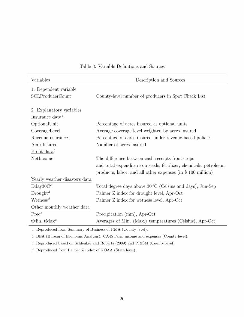
Table 3: Variable Definitions and Sources
Variables Description and Sources
1. Dependent variable
SCLProducerCount County-level number of producers in Spot Check List
2. Explanatory variables
Insurance dataa
OptionalUnit Percentage of acres insured as optional units
CoverageLevel Average coverage level weighted by acres insured
RevenueInsurance Percentage of acres insured under revenue-based policies
AcresInsured Number of acres insured
Profit datab
NetIncome The difference between cash receipts from crops
and total expenditure on seeds, fertilizer, chemicals, petroleum
products, labor, and all other expenses (in $ 100 million)
Yearly weather disasters data
Dday30Cc Total degree days above 30 ◦C (Celsius and days), Jun-Sep
Droughtd Palmer Z index for drought level, Apr-Oct
Wetnessd Palmer Z index for wetness level, Apr-Oct
Other monthly weather data
Precc Precipitation (mm), Apr-Oct
tMin, tMaxc Averages of Min. (Max.) temperatures (Celsius), Apr-Oct
a. Reproduced from Summary of Business of RMA (County level).
b. BEA (Bureau of Economic Analysis): CA45 Farm income and expenses (County level).
c. Reproduced based on Schlenker and Roberts (2009) and PRISM (County level).
d. Reproduced from Palmer Z Index of NOAA (State level).
26

Table 4: Summary Statistics for the Full Sample
Variable Mean Std. Dev. Min. Max.
Dependent variableSCLProducerCount .70 2.20 .00 38.00Insurance dataOptionalUnit .44 .25 .00 1.00RevenueInsurance .64 .29 .00 1.00CoverageLevel .67 .07 .50 .85AcresInsured 92,142.61 110,188.30 2.00 1,740,836.00Profit dataNetIncome -.19 .43 -6.42 13.74Yearly Weather dataDday30C 11.44 13.54 .00 138.43Drought .73 .61 .00 3.62Wetness 1.02 .78 .00 3.78Other Monthly Weather dataApr prec 89.48 55.29 .63 584.87May prec 103.69 60.79 .47 555.21Jun prec 106.52 60.79 .22 728.44Jul prec 95.41 56.10 .37 452.25Aug prec 89.93 56.31 .29 500.61Sep prec 84.66 60.61 .66 536.09Oct prec 79.18 56.13 .90 552.78Apr tMin 5.57 4.42 -8.38 20.94May tMin 10.90 4.05 -1.42 23.53Jun tMin 16.07 3.62 3.34 24.98Jul tMin 18.17 3.16 6.80 28.68Aug tMin 17.33 3.48 5.17 27.65Sep tMin 13.19 3.92 .46 25.09Oct tMin 6.70 4.12 -5.48 21.56Apr tMax 19.29 4.76 1.54 34.33May tMax 24.04 3.88 11.38 37.88Jun tMax 28.78 3.43 17.88 42.16Jul tMax 30.95 2.94 21.08 43.66Aug tMax 30.34 3.17 20.24 43.59Sep tMax 26.71 3.39 16.39 40.52Oct tMax 19.88 4.57 5.13 36.18
Note: All variables have 29,799 observations from 2,162 counties and years 2002-2015.
27

Table 5: Summary Statistics for the Per Acre Subsidy Variables from 2002 to 2015
Variable Obs. Mean Std. Dev. Min. Max.
Optional+Low Level+Revenue 24,701 18.053 10.972 0.562 174.050Optional+Low Level+Yield 26,113 15.184 17.480 0.832 312.778Optional+High Level+Revenue 25,996 25.836 13.463 4.227 184.789Optional+High Level+Yield 23,218 25.233 40.221 2.562 1,211.684NonOptional+Low Level+Revenue 26,429 15.765 9.750 1.199 108.333NonOptional+Low Level+Yield 28,912 9.427 19.937 0.338 901.853NonOptional+High Level+Revenue 27,133 25.591 14.410 2.867 169.497NonOptional+High Level+Yield 25,397 24.642 46.502 1.857 1,311.519
28
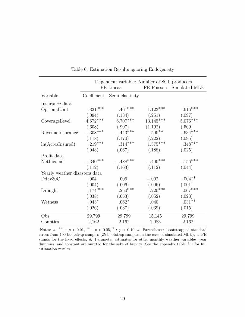
Table 6: Estimation Results ignoring Endogeneity
Dependent variable: Number of SCL producersFE Linear FE Poisson Simulated MLE
Variable Coefficient Semi-elasticity
Insurance dataOptionalUnit .321∗∗∗ .461∗∗∗ 1.123∗∗∗ .616∗∗∗
(.094) (.134) (.251) (.097)CoverageLevel 4.672∗∗∗ 6.707∗∗∗ 13.145∗∗∗ 5.076∗∗∗
(.608) (.907) (1.192) (.569)RevenueInsurance −.308∗∗∗ −.443∗∗∗ −.500∗∗ −.634∗∗∗
(.118) (.170) (.222) (.095)ln(AcresInsured) .219∗∗∗ .314∗∗∗ 1.575∗∗∗ .348∗∗∗
(.048) (.067) (.188) (.025)Profit dataNetIncome −.340∗∗∗ −.488∗∗∗ −.400∗∗∗ −.156∗∗∗
(.112) (.163) (.112) (.044)Yearly weather disasters dataDday30C .004 .006 −.002 .004∗∗
(.004) (.006) (.006) (.001)Drought .174∗∗∗ .250∗∗∗ .220∗∗∗ .067∗∗∗
(.038) (.053) (.052) (.023)Wetness .043∗ .062∗ .040 .031∗∗
(.026) (.037) (.039) (.015)
Obs. 29,799 29,799 15,145 29,799Counties 2,162 2,162 1,083 2,162
Notes: a. *** : p < 0.01, ** : p < 0.05, * : p < 0.10, b. Parentheses: bootstrapped standarderrors from 100 bootstrap samples (25 bootstrap samples in the case of simulated MLE), c. FEstands for the fixed effects, d. Parameter estimates for other monthly weather variables, yeardummies, and constant are omitted for the sake of brevity. See the appendix table A.1 for fullestimation results.
29
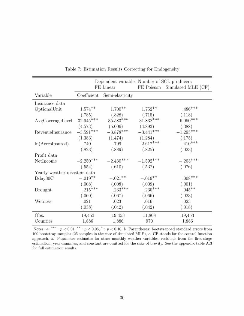
Table 7: Estimation Results Correcting for Endogeneity
Dependent variable: Number of SCL producersFE Linear FE Poisson Simulated MLE (CF)
Variable Coefficient Semi-elasticity
Insurance dataOptionalUnit 1.574∗∗ 1.700∗∗ 1.752∗∗ .486∗∗∗
(.785) (.828) (.715) (.118)AvgCoverageLevel 32.945∗∗∗ 35.583∗∗∗ 31.838∗∗∗ 6.050∗∗∗
(4.573) (5.006) (4.893) (.388)RevenueInsurance −3.591∗∗∗ −3.878∗∗∗ −3.441∗∗∗ −1.295∗∗∗
(1.383) (1.474) (1.284) (.175)ln(AcresInsured) .740 .799 2.617∗∗∗ .410∗∗∗
(.823) (.889) (.825) (.023)Profit dataNetIncome −2.250∗∗∗ −2.430∗∗∗ −1.592∗∗∗ −.203∗∗∗
(.554) (.610) (.532) (.076)Yearly weather disasters dataDday30C −.019∗∗ −.021∗∗ −.019∗∗ .008∗∗∗
(.008) (.008) (.009) (.001)Drought .215∗∗∗ .233∗∗∗ .230∗∗∗ .045∗∗
(.060) (.067) (.066) (.023)Wetness .021 .023 .016 .023
(.038) (.042) (.042) (.018)
Obs. 19,453 19,453 11,808 19,453Counties 1,886 1,886 970 1,886
Notes: a. *** : p < 0.01, ** : p < 0.05, * : p < 0.10, b. Parentheses: bootstrapped standard errors from100 bootstrap samples (25 samples in the case of simulated MLE), c. CF stands for the control functionapproach, d. Parameter estimates for other monthly weather variables, residuals from the first-stageestimation, year dummies, and constant are omitted for the sake of brevity. See the appendix table A.3for full estimation results.
30

Figure 1: Example of Unit Structure
31
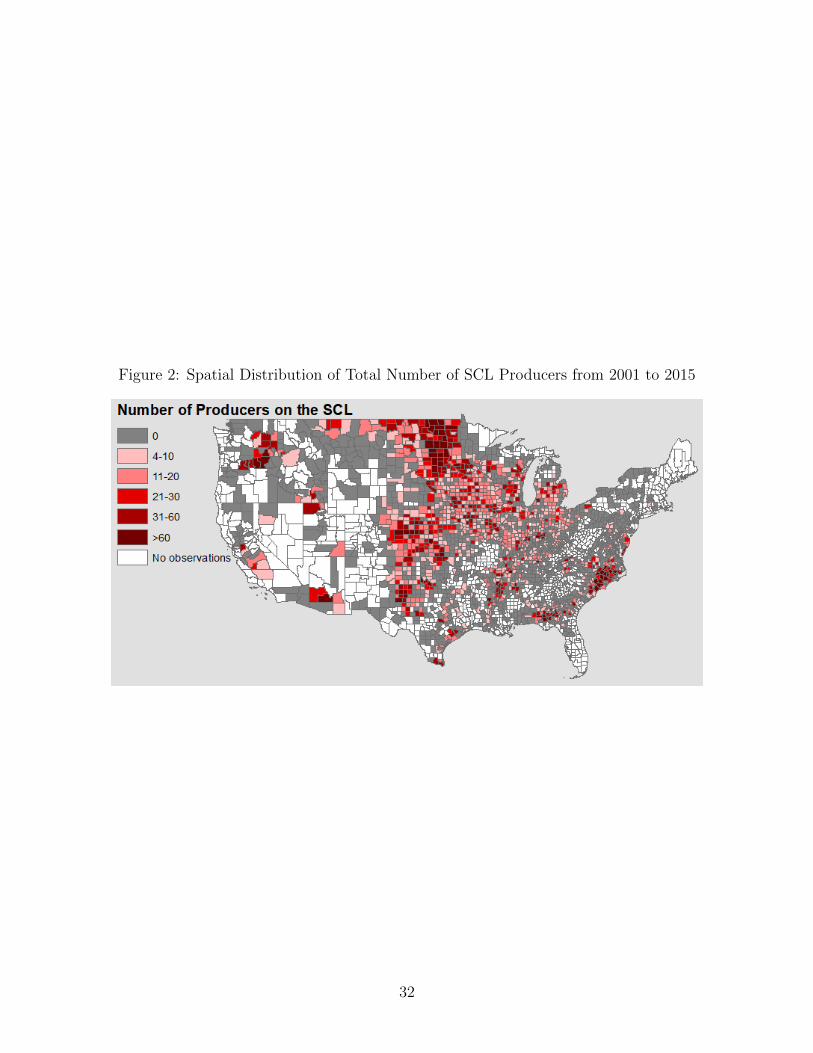
Figure 2: Spatial Distribution of Total Number of SCL Producers from 2001 to 2015
32

Figure 3: Spatial Distributions of Number of SCL Producers for Selected Years between 2001 and 2010

Figure 4: Spatial Distributions of Number of SCL Producers from 2012 to 2015

Figure 5: Percentages of Acres Insured as Different Types of Units from 2002 to 2015
35

Figure 6: Percentages of Acres Insured as Optional Units by Crop from 2002 to 2015
Figure 7: Spatial Distribution of Percentages of Acres Insured as Optional Units from 2002to 2015
36

Figure 8: Average Coverage Levels from 2002 to 2015
Figure 9: Spatial Distribution of Average Coverage Levels from 2002 to 2015
37

Figure 10: Percentages of Acres Insured under Revenue-based Policies from 2002 to 2015
Figure 11: Spatial Distribution of Percentages of Acres Insured under Revenue-based Policiesfrom 2002 to 2015
38
Appendix: Additional Results
Table A.1: Full Estimation Results for Table 6
Dependent variable: Number of SCL producersFE Linear FE Poisson Simulated MLE
Variable Coefficient Semi-elasticity
Insurance dataOptionalUnit .321∗∗∗ .461∗∗∗ 1.123∗∗∗ .616∗∗∗
(.094) (.134) (.251) (.097)CoverageLevel 4.672∗∗∗ 6.707∗∗∗ 13.145∗∗∗ 5.076∗∗∗
(.608) (.907) (1.192) (.569)RevenueInsurance −.308∗∗∗ −.443∗∗∗ −.500∗∗ −.634∗∗∗
(.118) (.170) (.222) (.095)ln(AcresInsured) .219∗∗∗ .314∗∗∗ 1.575∗∗∗ .348∗∗∗
(.048) (.067) (.188) (.025)Profit dataNetIncome −.340∗∗∗ −.488∗∗∗ −.400∗∗∗ −.156∗∗∗
(.112) (.163) (.112) (.044)Yearly weather disasters dataDday30C .004 .006 −.002 .004∗∗
(.004) (.006) (.006) (.001)Drought .174∗∗∗ .250∗∗∗ .220∗∗∗ .067∗∗∗
(.038) (.053) (.052) (.023)Wetness .043∗ .062∗ .040 .031∗∗
(.026) (.037) (.039) (.015)Other monthly weather dataln(Apr prec) .040 .058 .011
(.028) (.041) (.044)ln(May prec) −.094∗∗∗ −.135∗∗∗ −.121∗∗∗
(.025) (.035) (.041)ln(Jun prec) .102∗∗∗ .146∗∗∗ .189∗∗∗
(.034) (.049) (.048)ln(Jul prec) −.169∗∗∗ −.243∗∗∗ −.217∗∗∗
(.032) (.047) (.039)ln(Aug prec) −.160∗∗∗ −.229∗∗∗ −.167∗∗∗
(.029) (.044) (.040)ln(Sep prec) .060∗∗∗ .087∗∗∗ .056
(.023) (.033) (.036)ln(Oct prec) .063∗∗∗ .091∗∗∗ .128∗∗∗
(.023) (.033) (.036)Apr tMin −.022 −.031 −.004
(.015) (.021) (.027)May tMin .097∗∗∗ .139∗∗∗ .160∗∗∗
39

Table A.1 (continued)
Dependent variable: Number of SCL producersFE Linear FE Poisson Simulated MLE
Variable Coefficient Semi-elasticity
(.015) (.021) (.028)Jun tMin −.033 −.047 −.143∗∗∗
(.023) (.033) (.036)Jul tMin .026 .038 .085∗∗
(.019) (.027) (.036)Aug tMin −.025 −.036 −.064∗∗
(.019) (.028) (.031)Sep tMin −.050∗∗∗ −.072∗∗∗ −.072∗∗∗
(.015) (.022) (.027)Oct tMin −.055∗∗∗ −.080∗∗∗ −.099∗∗∗
(.016) (.022) (.026)Apr tMax −.032∗∗ −.046∗∗ −.038∗
(.013) (.019) (.020)May tMax −.059∗∗∗ −.085∗∗∗ −.110∗∗∗
(.014) (.020) (.028)Jun tMax .021 .030 .104∗∗∗
(.019) (.028) (.029)Jul tMax .025 .036 .057∗
(.020) (.029) (.029)Aug tMax −.036∗∗ −.052∗∗ −.025
(.018) (.026) (.024)Sep tMax −.004 −.006 .004
(.014) (.020) (.021)Oct tMax .043∗∗∗ .062∗∗∗ .045∗
(.016) (.023) (.024)Year and ConstantYear 2003 .079 .114 .212∗
(.080) (.114) (.117)Year 2004 .013 .018 .308∗
(.096) (.138) (.160)Year 2005 −.079 −.113 .024
(.064) (.093) (.098)Year 2006 −.504∗∗∗ −.723∗∗∗ −.889∗∗∗
(.089) (.130) (.148)Year 2007 −.054 −.077 .165
(.095) (.136) (.138)Year 2008 −.161 −.231 −.927∗∗∗
(.113) (.162) (.192)Year 2009 −.152∗ −.218∗ −.106
(.085) (.121) (.135)Year 2010 −.317∗∗∗ −.455∗∗∗ −.407∗∗∗
(.106) (.151) (.145)
40

Table A.1 (continued)
Dependent variable: Number of SCL producersFE Linear FE Poisson Simulated MLE
Variable Coefficient Semi-elasticity
Year 2011 −.523∗∗∗ −.750∗∗∗ −.774∗∗∗(.108) (.154) (.132)
Year 2012 −.603∗∗∗ −.865∗∗∗ −1.225∗∗∗(.103) (.148) (.155)
Year 2013 −.113 −.162 −.256∗(.104) (.149) (.154)
Year 2014 −.067 −.096 −.066(.120) (.172) (.166)
Year 2015 −.351∗∗∗ −.504∗∗∗ −.569∗∗∗(.111) (.158) (.166)
Constant −2.471∗∗ −4.849∗∗∗(1.084) (.308)
Obs. 29,799 29,799 15,145 29,799Counties 2,162 2,162 1,083 2,162
Notes: a. *** : p < 0.01, ** : p < 0.05, * : p < 0.10, b. Parentheses: bootstrapped standard
errors from 100 bootstrap samples (25 samples in the case of simulated MLE), c. FE stands
for the fixed effects.
41

Table A.2: Estimation Results of the First-Stage Regression
Dependent VariableVariable Optional Level Revenue ln(Acres) NetIncome
First-lagged subsidy variablesL ln(Opt+Low+Yield) .003 −.008∗∗∗ −.017∗∗∗ −.065∗∗∗ −.011
(.005) (.001) (.004) (.011) (.008)L ln(Opt+High+Revenue) .013 −.007∗∗∗ −.052∗∗∗ −.018 −.004
(.008) (.002) (.010) (.013) (.019)L ln(NonOpt+Low+Revenue) −.012∗∗ −.010∗∗∗ −.008 −.028∗∗∗ .021∗
(.006) (.001) (.006) (.009) (.012)L ln(NonOpt+Low+Yield) −.002 −.004∗∗∗ −.020∗∗∗ .019∗ .013
(.006) (.001) (.006) (.011) (.013)L ln(NonOpt+High+Revenue) −.113∗∗∗ .006∗∗∗ .008 .056∗∗∗ −.030
(.009) (.002) (.009) (.013) (.023)L ln(NonOpt+High+Yield) −.027∗∗∗ .001 .011∗∗ .011 .014∗∗
(.004) (.001) (.004) (.007) (.007)First-lagged yearly weather variablesL Dday30C −.001∗∗∗ .001∗∗∗ .003∗∗∗ .001∗∗∗ −.004∗∗∗
(.000) (.000) (.000) (.000) (.001)L Drought −.015∗∗∗ .004∗∗∗ −.005∗ −.023∗∗∗ −.056∗∗∗
(.002) (.000) (.002) (.004) (.008)L Wetness .000 .002∗∗∗ −.002 −.004∗∗ −.009∗∗∗
(.002) (.000) (.002) (.002) (.003)Other monthly weather variablesL ln Apr prec −.001 .001∗∗ −.006∗∗∗ .012∗∗∗ −.001
(.002) (.000) (.002) (.003) (.004)L ln May prec .004∗ −.002∗∗∗ −.003 −.003 −.022∗∗∗
(.002) (.000) (.002) (.003) (.004)L ln Jun prec −.005∗∗∗ .002∗∗∗ −.005∗∗∗ .009∗∗∗ .015∗∗
(.002) (.000) (.002) (.003) (.007)L ln Jul prec .000 .001∗∗ .011∗∗∗ .000 −.006
(.002) (.000) (.002) (.003) (.004)L ln Aug prec .008∗∗∗ −.005∗∗∗ −.018∗∗∗ −.006∗∗ −.024∗∗∗
(.002) (.000) (.002) (.003) (.004)L ln Sep prec .011∗∗∗ .000 −.001 −.002 −.009∗
(.001) (.000) (.002) (.002) (.005)L ln Oct prec −.005∗∗∗ .002∗∗∗ .005∗∗∗ .018∗∗∗ .007∗∗
(.001) (.000) (.002) (.002) (.003)L Apr tMin .001 .000∗ .004∗∗∗ −.004∗∗ .009∗∗
(.001) (.000) (.001) (.002) (.004)L May tMin −.010∗∗∗ .001∗∗∗ .009∗∗∗ .009∗∗∗ −.006∗∗
(.001) (.000) (.001) (.002) (.003)L Jun tMin .001 .005∗∗∗ .018∗∗∗ .016∗∗∗ −.011∗∗∗
(.002) (.000) (.002) (.002) (.004)L Jul tMin .004∗∗∗ −.004∗∗∗ −.011∗∗∗ −.015∗∗∗ −.003
42

Table A.2 (continued)
Variable Optional Level Revenue ln(Acres) NetIncome
(.001) (.000) (.001) (.002) (.005)L Aug tMin .003∗∗ .001∗∗∗ −.003∗∗ −.011∗∗∗ .007∗
(.001) (.000) (.001) (.002) (.004)L Sep tMin .005∗∗∗ .001∗∗∗ .005∗∗∗ −.003∗ −.004
(.001) (.000) (.001) (.002) (.005)L Oct tMin .001 −.001∗∗∗ −.006∗∗∗ −.003∗ .010∗∗
(.001) (.000) (.001) (.002) (.005)L Apr tMax .007∗∗∗ −.001∗∗∗ .000 .000 .000
(.001) (.000) (.001) (.001) (.002)L May tMax −.003∗∗∗ .001∗∗ −.003∗∗∗ .008∗∗∗ −.002
(.001) (.000) (.001) (.002) (.003)L Jun tMax .010∗∗∗ −.004∗∗∗ −.012∗∗∗ −.005∗∗ .019∗∗∗
(.002) (.000) (.002) (.002) (.004)L Jul tMax .000 .003∗∗∗ .010∗∗∗ .003 .006∗
(.001) (.000) (.001) (.002) (.003)L Aug tMax .000 −.002∗∗∗ −.012∗∗∗ −.004∗∗ −.006∗∗
(.001) (.000) (.001) (.002) (.003)L Sep tMax .005∗∗∗ −.002∗∗∗ −.006∗∗∗ −.011∗∗∗ −.008∗∗∗
(.001) (.000) (.001) (.002) (.002)L Oct tMax −.004∗∗∗ .002∗∗∗ .005∗∗∗ .005∗∗∗ −.003
(.001) (.000) (.001) (.001) (.003)
F-statistics 120.75 177.34 120.50 2,073.99 37.58(p-value) (.000) (.000) (.000) (.000) (.000)Obs. 19,453 19,453 19,453 19,453 19,453Counties 1,886 1,886 1,886 1,886 1,886
Notes: a. *** : p < 0.01, ** : p < 0.05, * : p < 0.10, b. Parenthesis: county-level clustered robust
standard errors, c. Parameter estimates for exogenous variables in the main model, year dummies,
and constant are omitted for the sake of brevity.
43

Table A.3: Full Estimation Results for Table 7
Dependent variable: Number of SCL producers2SLS FE Poisson (CF) Simulated MLE (CF)
Variable Coefficient Semi-elasticity
Insurance dataOptionalUnit 1.574∗∗ 1.700∗∗ 1.752∗∗ .486∗∗∗
(.785) (.828) (.715) (.118)AvgCoverageLevel 32.945∗∗∗ 35.583∗∗∗ 31.838∗∗∗ 6.050∗∗∗
(4.573) (5.006) (4.893) (.388)RevenueInsurance −3.591∗∗∗ −3.878∗∗∗ −3.441∗∗∗ −1.295∗∗∗
(1.383) (1.474) (1.284) (.175)ln(AcresInsured) .740 .799 2.617∗∗∗ .410∗∗∗
(.823) (.889) (.825) (.023)Profit dataNetIncome −2.250∗∗∗ −2.430∗∗∗ −1.592∗∗∗ −.203∗∗∗
(.554) (.610) (.532) (.076)Yearly weather disasters dataDday30C −.019∗∗ −.021∗∗ −.019∗∗ .008∗∗∗
(.008) (.008) (.009) (.001)Drought .215∗∗∗ .233∗∗∗ .230∗∗∗ .045∗∗
(.060) (.067) (.066) (.023)Wetness .021 .023 .016 .023
(.038) (.042) (.042) (.018)Other Monthly weather dataln(Apr prec) −.030 −.032 −.101∗∗
(.039) (.042) (.050)ln(May prec) −.015 −.016 −.006
(.045) (.049) (.050)ln(Jun prec) .146∗∗∗ .158∗∗∗ .207∗∗∗
(.053) (.059) (.047)ln(Jul prec) −.218∗∗∗ −.235∗∗∗ −.212∗∗∗
(.044) (.050) (.047)ln(Aug prec) −.051 −.056 −.057
(.040) (.043) (.050)ln(Sep prec) .017 .019 .023
(.038) (.041) (.039)ln(Oct prec) .086∗∗ .093∗∗ .119∗∗∗
(.034) (.037) (.038)Apr tMin .000 .000 .038
(.028) (.030) (.030)May tMin .037 .040 .079∗∗
(.028) (.030) (.034)Jun tMin −.122∗∗∗ −.132∗∗∗ −.183∗∗∗
(.034) (.038) (.038)Jul tMin .131∗∗∗ .141∗∗∗ .155∗∗∗
44

Table A.3 (continued)
Dependent variable: Number of SCL producers2SLS FE Poisson (CF) Simulated MLE (CF)
Variable Coefficient Semi-elasticity
(.033) (.038) (.037)Aug tMin −.134∗∗∗ −.144∗∗∗ −.133∗∗∗
(.030) (.034) (.034)Sep tMin −.078∗∗∗ −.085∗∗∗ −.071∗∗
(.025) (.028) (.031)Oct tMin −.037 −.040 −.053∗
(.027) (.029) (.030)Apr tMax −.067∗∗∗ −.073∗∗∗ −.065∗∗∗
(.021) (.023) (.023)May tMax −.070∗∗ −.076∗∗ −.106∗∗∗
(.027) (.030) (.032)Jun tMax .101∗∗∗ .109∗∗∗ .150∗∗∗
(.030) (.034) (.031)Jul tMax .052∗ .056∗ .066∗∗
(.028) (.031) (.033)Aug tMax .053∗∗ .057∗ .058∗∗
(.027) (.030) (.027)Sep tMax .015 .016 .019
(.023) (.025) (.026)Oct tMax .006 .006 −.006
(.022) (.024) (.025)Year and ConstantYear2004 .194 .210 .301
(.169) (.184) (.196)Year2005 −.379∗∗∗ −.409∗∗∗ −.324∗
(.125) (.138) (.175)Year2006 −.733∗∗∗ −.792∗∗∗ −.973∗∗∗
(.134) (.149) (.159)Year2007 .227 .246 .297
(.193) (.210) (.214)Year2008 −.353 −.381 −1.590∗∗
(.625) (.675) (.622)Year2009 −.240 −.259 −.295
(.194) (.210) (.198)Year2010 −.176 −.191 −.378
(.297) (.322) (.297)Year2011 −.725∗∗ −.783∗∗ −.933∗∗∗
(.314) (.348) (.317)Year2012 −1.127∗∗∗ −1.218∗∗∗ −1.495∗∗∗
(.346) (.390) (.319)Year2013 −.610∗ −.659∗ −.721∗∗
(.355) (.391) (.355)
45
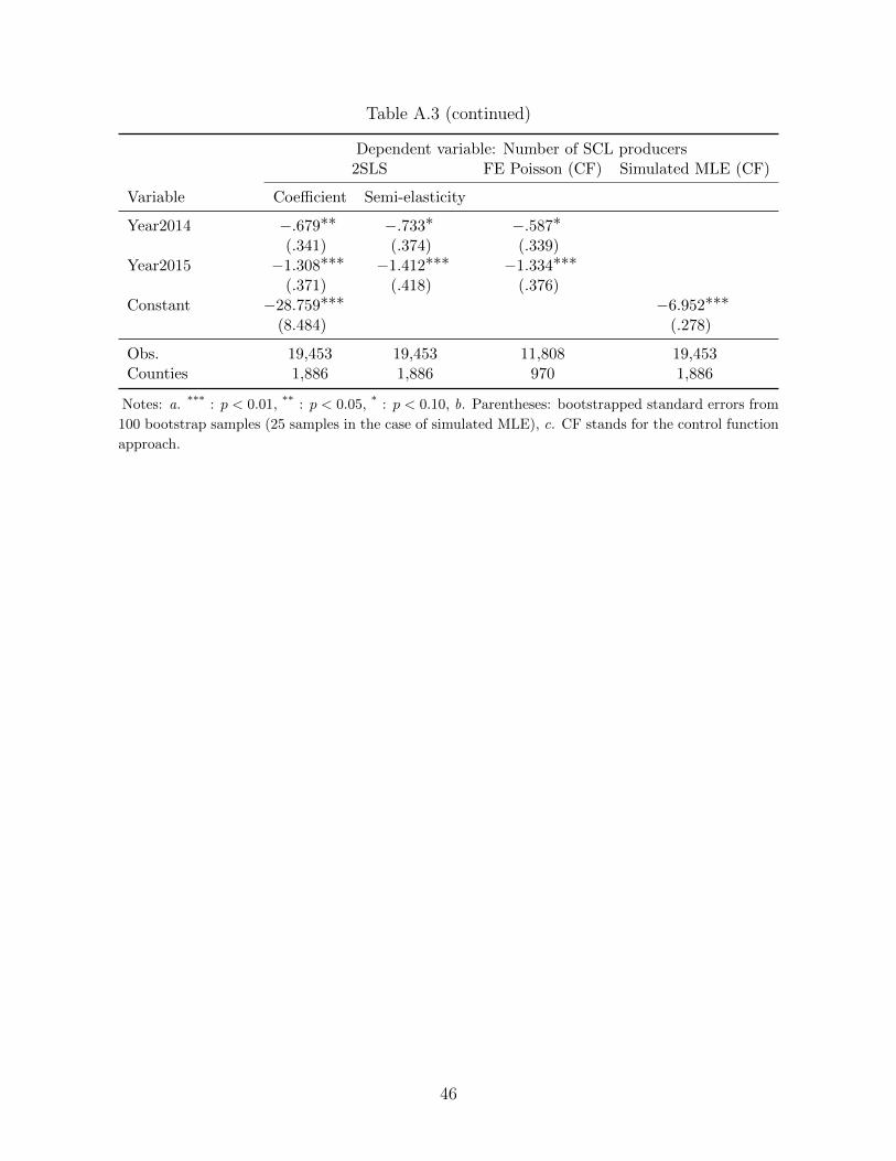
Table A.3 (continued)
Dependent variable: Number of SCL producers2SLS FE Poisson (CF) Simulated MLE (CF)
Variable Coefficient Semi-elasticity
Year2014 −.679∗∗ −.733∗ −.587∗(.341) (.374) (.339)
Year2015 −1.308∗∗∗ −1.412∗∗∗ −1.334∗∗∗(.371) (.418) (.376)
Constant −28.759∗∗∗ −6.952∗∗∗(8.484) (.278)
Obs. 19,453 19,453 11,808 19,453Counties 1,886 1,886 970 1,886
Notes: a. *** : p < 0.01, ** : p < 0.05, * : p < 0.10, b. Parentheses: bootstrapped standard errors from
100 bootstrap samples (25 samples in the case of simulated MLE), c. CF stands for the control function
approach.
46