continuous wavelet transform matlab & simulink

8/28/2015 Continuous Wavelet Transform MATLAB & Simulink

http://www.mathworks.com/help/wavelet/gs/continuouswavelettransform.html 1/30

Continuous Wavelet Transform

Definition of the Continuous Wavelet TransformLike the Fourier transform, the continuous wavelet transform (CWT) uses inner products to measure the similarity between

a signal and an analyzing function. In the Fourier transform, the analyzing functions are complex exponentials, . Theresulting transform is a function of a single variable, ω. In the shorttime Fourier transform, the analyzing functions are

windowed complex exponentials, , and the result in a function of two variables. The STFT coefficients, represent the match between the signal and a sinusoid with angular frequency ω in an interval of a specified lengthcentered at τ.

In the CWT, the analyzing function is a wavelet, ψ. The CWT compares the signal to shifted and compressed or stretchedversions of a wavelet. Stretching or compressing a function is collectively referred to as dilation or scaling and correspondsto the physical notion of scale. By comparing the signal to the wavelet at various scales and positions, you obtain afunction of two variables. The twodimensional representation of a onedimensional signal is redundant. If the wavelet iscomplexvalued, the CWT is a complexvalued function of scale and position. If the signal is realvalued, the CWT is a realvalued function of scale and position. For a scale parameter, a>0, and position, b, the CWT is:

where denotes the complex conjugate. Not only do the values of scale and position affect the CWT coefficients, thechoice of wavelet also affects the values of the coefficients.

By continuously varying the values of the scale parameter, a, and the position parameter, b, you obtain the cwt coefficientsC(a,b). Note that for convenience, the dependence of the CWT coefficients on the function and analyzing wavelet has beensuppressed.

Multiplying each coefficient by the appropriately scaled and shifted wavelet yields the constituent wavelets of the originalsignal.

There are many different admissible wavelets that can be used in the CWT. While it may seem confusing that there are somany choices for the analyzing wavelet, it is actually a strength of wavelet analysis. Depending on what signal featuresyou are trying to detect, you are free to select a wavelet that facilitates your detection of that feature. For example, if you aretrying to detect abrupt discontinuities in your signal, you may choose one wavelet. On the other hand, if you are interestingin finding oscillations with smooth onsets and offsets, you are free to choose a wavelet that more closely matches thatbehavior.

ScaleLike the concept of frequency, scale is another useful property of signals and images. For example, you can analyzetemperature data for changes on different scales. You can look at yeartoyear or decadetodecade changes. Of course,you can examine finer (daytoday), or coarser scale changes as well. Some processes reveal interesting changes on longtime, or spatial scales that are not evident on small time or spatial scales. The opposite situation also happens. Some ofour perceptual abilities exhibit scale invariance. You recognize people you know regardless of whether you look at a largeportrait, or small photograph.

e jωt

w(t)e jωt F (ω, τ),

C(a, b; f (t), ψ(t)) =∞

−∞f (t) 1G

aψ∗(t−b

a) dt

∗



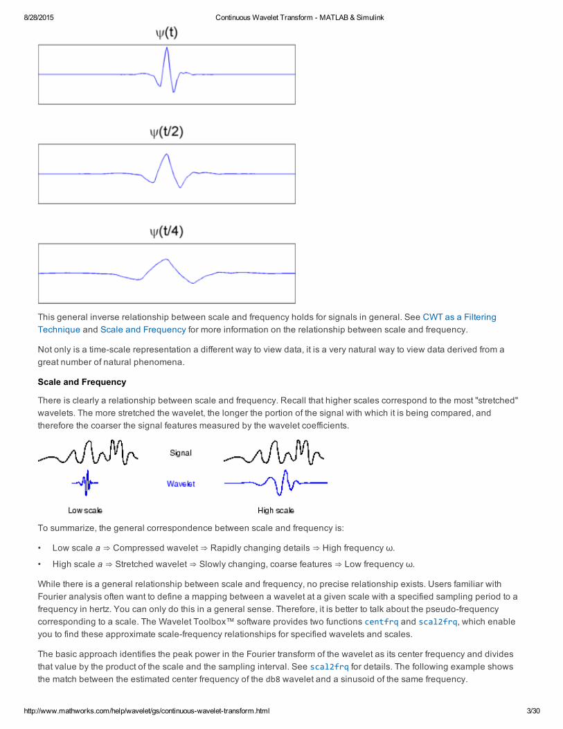
To go beyond colloquial descriptions such as "stretching" or "shrinking" we introduce the scale factor, often denoted by theletter a. The scale factor is a inherently positive quantity, a>0. For sinusoids, the effect of the scale factor is very easy tosee.

In sin(at), the scale is the inverse of the radian frequency, a.

The scale factor works exactly the same with wavelets. The smaller the scale factor, the more "compressed" the wavelet.Conversely, the larger the scale, the more stretched the wavelet. The following figure illustrates this for wavelets at scales1,2, and 4.



•

•

This general inverse relationship between scale and frequency holds for signals in general. See CWT as a FilteringTechnique and Scale and Frequency for more information on the relationship between scale and frequency.

Not only is a timescale representation a different way to view data, it is a very natural way to view data derived from agreat number of natural phenomena.

Scale and Frequency

There is clearly a relationship between scale and frequency. Recall that higher scales correspond to the most "stretched"wavelets. The more stretched the wavelet, the longer the portion of the signal with which it is being compared, andtherefore the coarser the signal features measured by the wavelet coefficients.

To summarize, the general correspondence between scale and frequency is:

Low scale a ⇒ Compressed wavelet ⇒ Rapidly changing details ⇒ High frequency ω.

High scale a ⇒ Stretched wavelet ⇒ Slowly changing, coarse features ⇒ Low frequency ω.

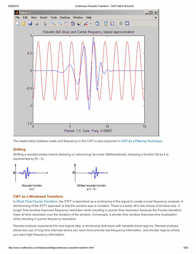
While there is a general relationship between scale and frequency, no precise relationship exists. Users familiar withFourier analysis often want to define a mapping between a wavelet at a given scale with a specified sampling period to afrequency in hertz. You can only do this in a general sense. Therefore, it is better to talk about the pseudofrequencycorresponding to a scale. The Wavelet Toolbox™ software provides two functions centfrq and scal2frq, which enableyou to find these approximate scalefrequency relationships for specified wavelets and scales.

The basic approach identifies the peak power in the Fourier transform of the wavelet as its center frequency and dividesthat value by the product of the scale and the sampling interval. See scal2frq for details. The following example showsthe match between the estimated center frequency of the db8 wavelet and a sinusoid of the same frequency.

http://www.mathworks.com/help/wavelet/ref/scal2frq.html

http://www.mathworks.com/help/wavelet/ref/scal2frq.html

http://www.mathworks.com/help/wavelet/ref/centfrq.html



The relationship between scale and frequency in the CWT is also explored in CWT as a Filtering Technique.

ShiftingShifting a wavelet simply means delaying (or advancing) its onset. Mathematically, delaying a function f(t) by k isrepresented by f(t – k):

CWT as a Windowed TransformIn ShortTime Fourier Transform, the STFT is described as a windowing of the signal to create a local frequency analysis. Ashortcoming of the STFT approach is that the window size is constant. There is a trade off in the choice of window size. Alonger time window improves frequency resolution while resulting in poorer time resolution because the Fourier transformloses all time resolution over the duration of the window. Conversely, a shorter time window improves time localizationwhile resulting in poorer frequency resolution.

Wavelet analysis represents the next logical step: a windowing technique with variablesized regions. Wavelet analysisallows the use of long time intervals where you want more precise lowfrequency information, and shorter regions whereyou want highfrequency information.

http://www.mathworks.com/help/wavelet/gs/from-fourier-analysis-to-wavelet-analysis.html#bsoozdn-3



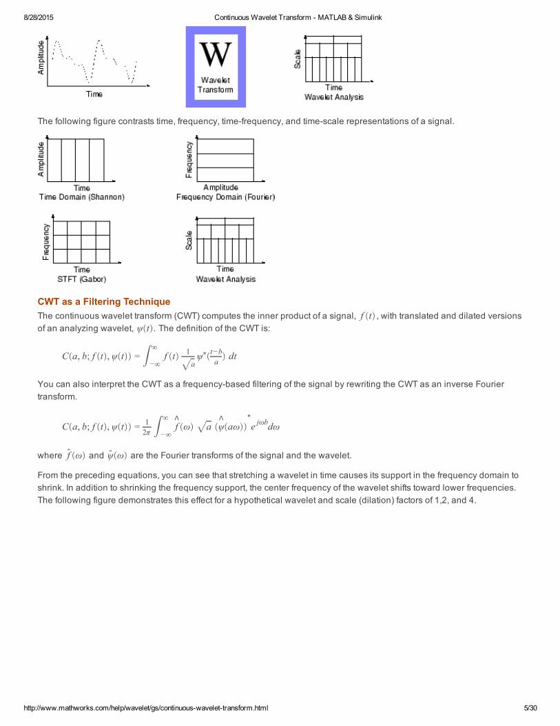
The following figure contrasts time, frequency, timefrequency, and timescale representations of a signal.

CWT as a Filtering TechniqueThe continuous wavelet transform (CWT) computes the inner product of a signal, , with translated and dilated versionsof an analyzing wavelet, The definition of the CWT is:

You can also interpret the CWT as a frequencybased filtering of the signal by rewriting the CWT as an inverse Fouriertransform.

where and are the Fourier transforms of the signal and the wavelet.

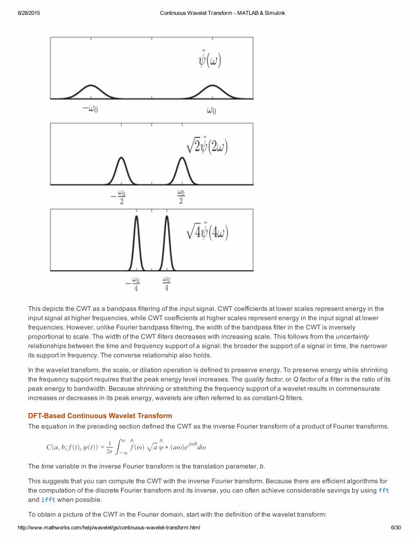
From the preceding equations, you can see that stretching a wavelet in time causes its support in the frequency domain toshrink. In addition to shrinking the frequency support, the center frequency of the wavelet shifts toward lower frequencies.The following figure demonstrates this effect for a hypothetical wavelet and scale (dilation) factors of 1,2, and 4.

f (t)ψ(t).

C(a, b; f (t), ψ(t)) =∞

−∞f (t) 1G

aψ∗(t−b

a) dt

C(a, b; f (t), ψ(t)) = 12π

∞

−∞

∧f (ω)

Ga (

∧ψ(aω))

∗e jωbdω

f (ω) ψ(ω)



This depicts the CWT as a bandpass filtering of the input signal. CWT coefficients at lower scales represent energy in theinput signal at higher frequencies, while CWT coefficients at higher scales represent energy in the input signal at lowerfrequencies. However, unlike Fourier bandpass filtering, the width of the bandpass filter in the CWT is inverselyproportional to scale. The width of the CWT filters decreases with increasing scale. This follows from the uncertaintyrelationships between the time and frequency support of a signal: the broader the support of a signal in time, the narrowerits support in frequency. The converse relationship also holds.

In the wavelet transform, the scale, or dilation operation is defined to preserve energy. To preserve energy while shrinkingthe frequency support requires that the peak energy level increases. The quality factor, or Q factor of a filter is the ratio of itspeak energy to bandwidth. Because shrinking or stretching the frequency support of a wavelet results in commensurateincreases or decreases in its peak energy, wavelets are often referred to as constantQ filters.

DFTBased Continuous Wavelet TransformThe equation in the preceding section defined the CWT as the inverse Fourier transform of a product of Fourier transforms.

The time variable in the inverse Fourier transform is the translation parameter, b.

This suggests that you can compute the CWT with the inverse Fourier transform. Because there are efficient algorithms forthe computation of the discrete Fourier transform and its inverse, you can often achieve considerable savings by using fftand ifft when possible.

To obtain a picture of the CWT in the Fourier domain, start with the definition of the wavelet transform:

C(a, b; f (t), ψ(t)) = 12π

∞

−∞

∧f (ω)

Ga∧ψ ∗ (aω)e jωbdω

∞

http://www.mathworks.com/help/matlab/ref/fft.html

http://www.mathworks.com/help/matlab/ref/ifft.html



If you define:

you can rewrite the wavelet transform as

which explicitly expresses the CWT as a convolution.

To implement the discretized verion of the CWT, assume that the input sequence is a length N vector, x[n]. The discreteversion of the preceding convolution is:

To obtain the CWT, it appears you have to compute the convolution for each value of the shift parameter, b, and repeat thisprocess for each scale, a.

However, if the two sequences are circularlyextended (periodized to length N), you can express the circular convolutionas a product of discrete Fourier transforms. The CWT is the inverse Fourier transform of the product

where Δt is the sampling interval (period).

Expressing the CWT as an inverse Fourier transform enables you to use the computationallyefficient fft and ifftalgorithms to reduce the cost of computing convolutions.

The cwtft function implements the CWT using an FFTbased algorithm. See cwtftinfo for information pertaining to thesupported analyzing wavelets.

Inverse Continuous Wavelet TransformThe icwtft function implements the inverse CWT. Using icwtft requires that you obtain the CWT from cwtft. TheWavelet Toolbox does not support the inverse CWT for a general CWT obtained using cwt.

Because the CWT is a redundant transform, there is not a unique way to define the inverse. The inverse CWT implementedin the Wavelet Toolbox utilizes a discrete version of the single integral formula due to Morlet.

The inverse CWT is classically presented in the doubleintegral form. Assume you have a wavelet with a Fourier transformthat satisfies the admissibility condition:

For wavelets satisfying the admissibility condition and finiteenergy functions, f(t), you can define the inverse CWT as:

For analyzing wavelets and functions satisfying the following conditions, a single integral formula for the inverse CWTexists. These conditions are:

< f (t), ψa,b(t) >=1Ga

∞

−∞f (t)ψ∗(t−b

a)dt

ψa(t) =1Gaψ∗(−t/a)

(f ∗ ψa)(b) =∞

−∞f (t)ψa(b − t)dt

W a[b] =N−1

n=0x[n] ψa[b − n]

W a(b) =1N

G2πaΔt

N−1

k=0

∧X (2πk/NΔt)

∧ψ ∗ (a2πk/NΔt)e j2πkb/N

Cψ =∞

−∞

|∧ψ(ω)|

2

|ω| dω < ∞

f (t) = 1Cψ

a

b< f (t), ψa,b(t) > ψa,b(t) db

da

a2

http://www.mathworks.com/help/wavelet/ref/cwtft.html

http://www.mathworks.com/help/wavelet/ref/cwt.html

http://www.mathworks.com/help/wavelet/ref/cwtftinfo.html


http://www.mathworks.com/help/matlab/ref/fft.html

http://www.mathworks.com/help/wavelet/ref/icwtft.html

http://www.mathworks.com/help/matlab/ref/ifft.html



•

•

The analyzed function, f(t), is realvalued and the analyzing wavelet has a realvalued Fourier transform.

The analyzed function, f(t), is realvalued and the Fourier transform of the analyzing wavelet has support only on the setof nonnegative frequencies. This is referred to as an analytic wavelet. A function whose Fourier transform only hassupport on the set of nonnegative frequencies must be complexvalued.

The preceding conditions constrain the set of possible analyzing wavelets. If you inspect the list of wavelets supported bycwtft, each wavelet is either analytic or has a realvalued Fourier transform. Because the toolbox only supports theanalysis of realvalued functions, the realvalued condition on the analyzed function is always satisfied.

To motivate the single integral formula, let ψ and ψ be two wavelets that satisfy the following twowavelet admissibilitycondition:

Define the constant:

INote that the above constant may be complexvalued. Let f(t) and g(t) be two finite energy functions. If the twowaveletadmissibility condition is satisfied, the following equality holds:

where < , > denotes the inner product, * denotes the complex conjugate, and the dependence of ψ and ψ on scale andposition has been suppressed for convenience.

The key to the single integral formula for the inverse CWT is to recognize that the twowavelet admissibility condition canbe satisfied even if one of the wavelets is not admissible. In other words, it is not necessary that both ψ and ψ beseparately admissible. You can also relax the requirements further by allowing one of the functions and wavelets to bedistributions. By first letting g(t) be the Dirac delta function (a distribution) and also allowing ψ to be the Dirac deltafunction, you can derive the single integral formula for the inverse CWT

where Re denotes the real part.

The preceding equation demonstrates that you can reconstruct the signal by summing the scaled CWT coefficients over allscales.

By summing the scaled CWT coefficients from select scales, you obtain an approximation to the original signal. This isuseful in situations where your phenomenon of interest is localized in scale.

icwtft implements a discretized version of the above integral.

Continuous Wavelet Transform AlgorithmThe following outlines the basic algorithm for the CWT:

1. Take a wavelet and compare it to a section at the start of the original signal.

1 2

∧ψ∗1(ω)

∧ψ2(ω)

ω

dω < ∞

Cψ1,ψ2=

∧ψ∗1(ω)

∧ψ2(ω)ω dω

Cψ1,ψ2< f, g >=

< f, ψ1 >< g, ψ2 >

∗ dbdaa2

1 2

1 2

2

f (t) = 2   Re

1Cψ1,δ

∞

0< f (t), ψ1(t) >

da

a3/2

http://www.mathworks.com/help/wavelet/ref/icwtft.html




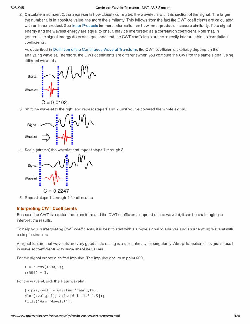
2. Calculate a number, C, that represents how closely correlated the wavelet is with this section of the signal. The largerthe number C is in absolute value, the more the similarity. This follows from the fact the CWT coefficients are calculatedwith an inner product. See Inner Products for more information on how inner products measure similarity. If the signalenergy and the wavelet energy are equal to one, C may be interpreted as a correlation coefficient. Note that, ingeneral, the signal energy does not equal one and the CWT coefficients are not directly interpretable as correlationcoefficients.

As described in Definition of the Continuous Wavelet Transform, the CWT coefficients explicitly depend on theanalyzing wavelet. Therefore, the CWT coefficients are different when you compute the CWT for the same signal usingdifferent wavelets.

3. Shift the wavelet to the right and repeat steps 1 and 2 until you've covered the whole signal.

4. Scale (stretch) the wavelet and repeat steps 1 through 3.

5. Repeat steps 1 through 4 for all scales.

Interpreting CWT CoefficientsBecause the CWT is a redundant transform and the CWT coefficients depend on the wavelet, it can be challenging tointerpret the results.

To help you in interpreting CWT coefficients, it is best to start with a simple signal to analyze and an analyzing wavelet witha simple structure.

A signal feature that wavelets are very good at detecting is a discontinuity, or singularity. Abrupt transitions in signals resultin wavelet coefficients with large absolute values.

For the signal create a shifted impulse. The impulse occurs at point 500.

x = zeros(1000,1);x(500) = 1;

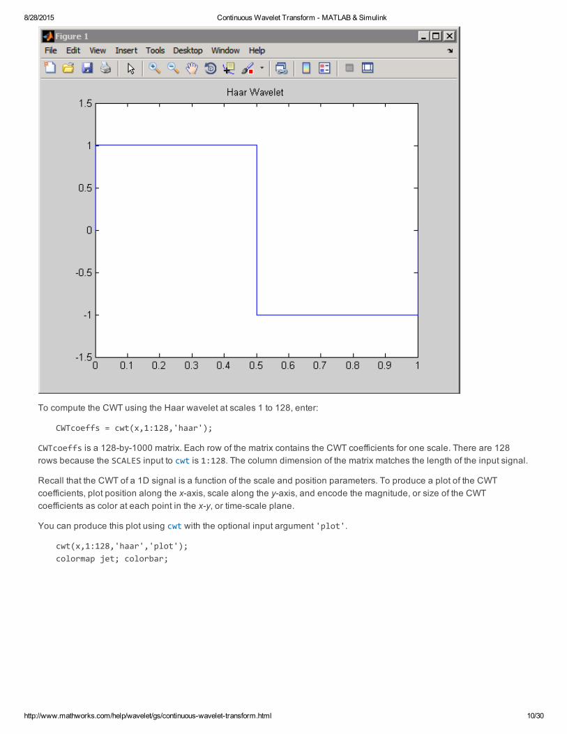
For the wavelet, pick the Haar wavelet.

[~,psi,xval] = wavefun('haar',10);plot(xval,psi); axis([0 1 ‐1.5 1.5]);title('Haar Wavelet');

http://www.mathworks.com/help/wavelet/gs/from-fourier-analysis-to-wavelet-analysis.html#bsos_xr



To compute the CWT using the Haar wavelet at scales 1 to 128, enter:

CWTcoeffs = cwt(x,1:128,'haar');

CWTcoeffs is a 128by1000 matrix. Each row of the matrix contains the CWT coefficients for one scale. There are 128rows because the SCALES input to cwt is 1:128. The column dimension of the matrix matches the length of the input signal.

Recall that the CWT of a 1D signal is a function of the scale and position parameters. To produce a plot of the CWTcoefficients, plot position along the xaxis, scale along the yaxis, and encode the magnitude, or size of the CWTcoefficients as color at each point in the xy, or timescale plane.

You can produce this plot using cwt with the optional input argument 'plot'.

cwt(x,1:128,'haar','plot'); colormap jet; colorbar;





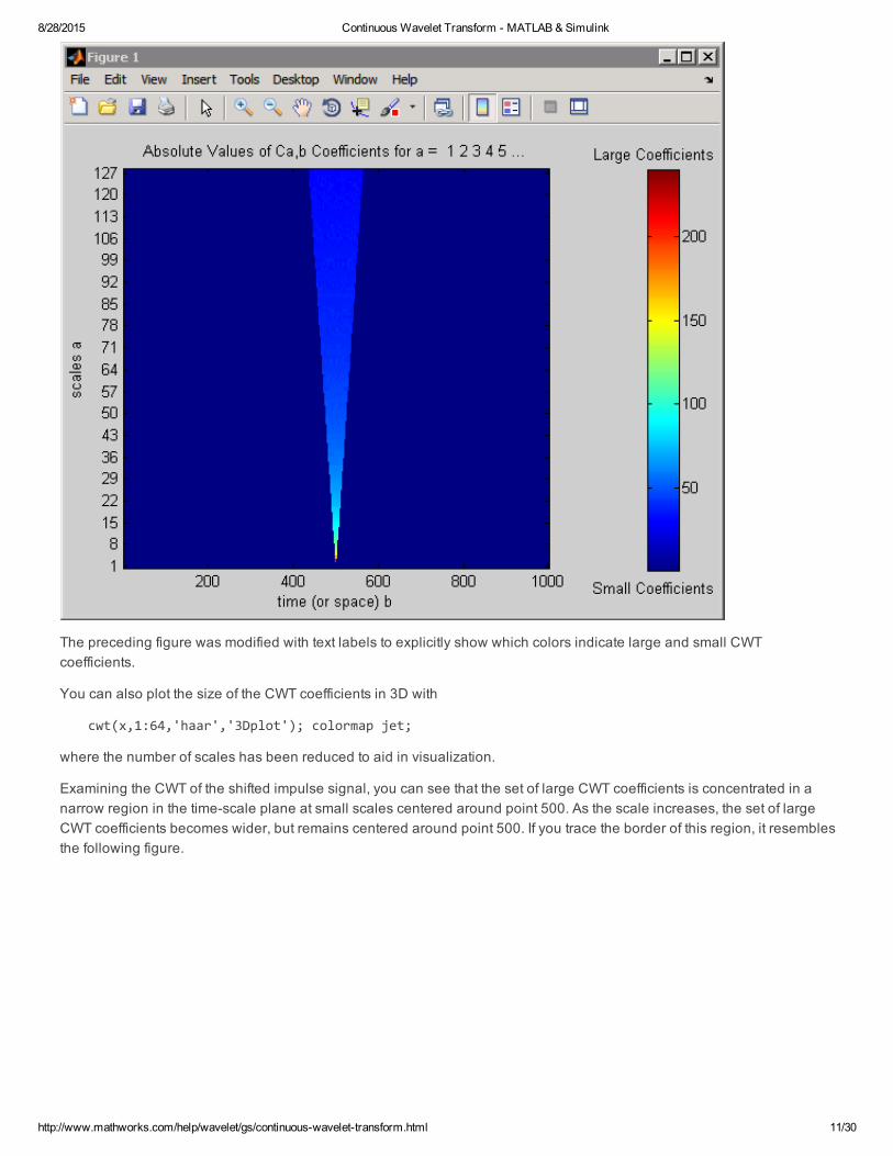
The preceding figure was modified with text labels to explicitly show which colors indicate large and small CWTcoefficients.

You can also plot the size of the CWT coefficients in 3D with

cwt(x,1:64,'haar','3Dplot'); colormap jet;

where the number of scales has been reduced to aid in visualization.

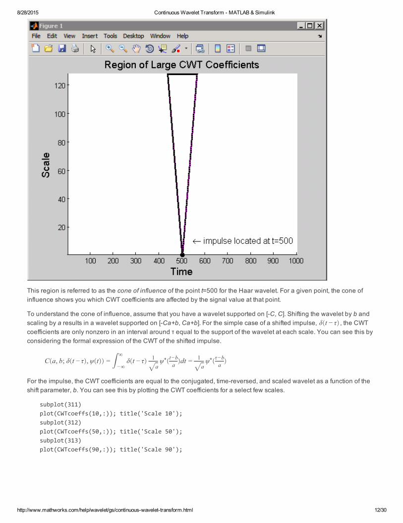
Examining the CWT of the shifted impulse signal, you can see that the set of large CWT coefficients is concentrated in anarrow region in the timescale plane at small scales centered around point 500. As the scale increases, the set of largeCWT coefficients becomes wider, but remains centered around point 500. If you trace the border of this region, it resemblesthe following figure.



This region is referred to as the cone of influence of the point t=500 for the Haar wavelet. For a given point, the cone ofinfluence shows you which CWT coefficients are affected by the signal value at that point.

To understand the cone of influence, assume that you have a wavelet supported on [C, C]. Shifting the wavelet by b andscaling by a results in a wavelet supported on [Ca+b, Ca+b]. For the simple case of a shifted impulse, , the CWTcoefficients are only nonzero in an interval around τ equal to the support of the wavelet at each scale. You can see this byconsidering the formal expression of the CWT of the shifted impulse.

For the impulse, the CWT coefficients are equal to the conjugated, timereversed, and scaled wavelet as a function of theshift parameter, b. You can see this by plotting the CWT coefficients for a select few scales.

subplot(311)plot(CWTcoeffs(10,:)); title('Scale 10');subplot(312)plot(CWTcoeffs(50,:)); title('Scale 50');subplot(313)plot(CWTcoeffs(90,:)); title('Scale 90');

δ(t − τ)

C(a, b; δ(t − τ), ψ(t)) =∞

−∞δ(t − τ) 1G

aψ∗(t−b

a)dt = 1G

aψ∗(τ−b

a)



The cone of influence depends on the wavelet. You can find and plot the cone of influence for a specific wavelet withconofinf.

The next example features the superposition of two shifted impulses, . In this case, use theDaubechies' extremal phase wavelet with four vanishing moments, db4. The following figure shows the cone of influencefor the points 300 and 500 using the db4 wavelet.

δ(t − 300) + δ(t − 500)

http://www.mathworks.com/help/wavelet/ref/conofinf.html



Look at point 400 for scale 20. At that scale, you can see that neither cone of influence overlaps the point 400. Therefore,you can expect that the CWT coefficient will be zero at that point and scale. The signal is only nonzero at two values, 300and 500, and neither cone of influence for those values includes the point 400 at scale 20. You can confirm this byentering:

x = zeros(1000,1);x([300 500]) = 1;CWTcoeffs = cwt(x,1:128,'db4');plot(CWTcoeffs(20,:)); grid on;



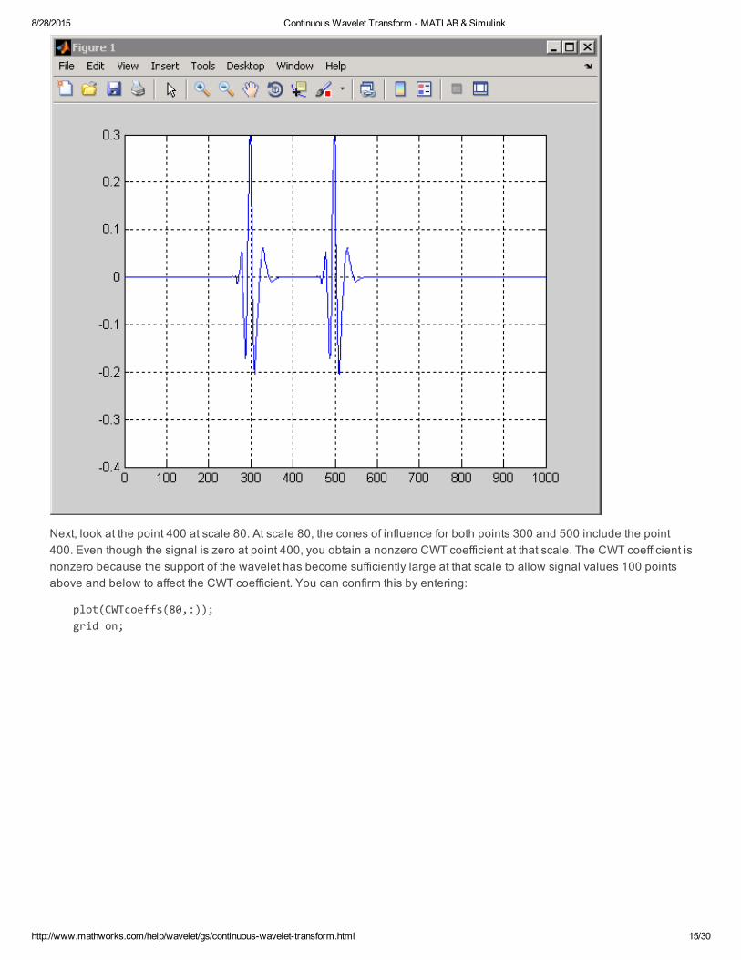
Next, look at the point 400 at scale 80. At scale 80, the cones of influence for both points 300 and 500 include the point400. Even though the signal is zero at point 400, you obtain a nonzero CWT coefficient at that scale. The CWT coefficient isnonzero because the support of the wavelet has become sufficiently large at that scale to allow signal values 100 pointsabove and below to affect the CWT coefficient. You can confirm this by entering:

plot(CWTcoeffs(80,:));grid on;



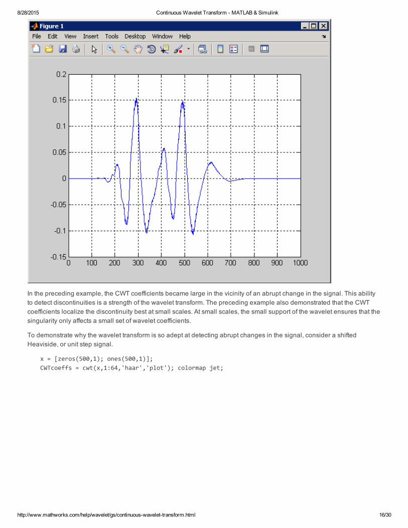
In the preceding example, the CWT coefficients became large in the vicinity of an abrupt change in the signal. This abilityto detect discontinuities is a strength of the wavelet transform. The preceding example also demonstrated that the CWTcoefficients localize the discontinuity best at small scales. At small scales, the small support of the wavelet ensures that thesingularity only affects a small set of wavelet coefficients.

To demonstrate why the wavelet transform is so adept at detecting abrupt changes in the signal, consider a shiftedHeaviside, or unit step signal.

x = [zeros(500,1); ones(500,1)];CWTcoeffs = cwt(x,1:64,'haar','plot'); colormap jet;



Similar to the shifted impulse example, the abrupt transition in the shifted step function results in large CWT coefficients atthe discontinuity. The following figure illustrates why this occurs.



In the preceding figure, the red function is the shifted unit step function. The black functions labeled A, B, and C depict Haarwavelets at the same scale but different positions. You can see that the CWT coefficients around position A are zero. Thesignal is zero in that neighborhood and therefore the wavelet transform is also zero because any wavelet integrates tozero.

Note the Haar wavelet centered around position B. The negative part of the Haar wavelet overlaps with a region of the stepfunction that is equal to 1. The CWT coefficients are negative because the product of the Haar wavelet and the unit step isa negative constant. Integrating over that area yields a negative number.

Note the Haar wavelet centered around position C. Here the CWT coefficients are zero. The step function is equal to one.The product of the wavelet with the step function is equal to the wavelet. Integrating any wavelet over its support is zero.This is the zero moment property of wavelets.

At position B, the Haar wavelet has already shifted into the nonzero portion of the step function by 1/2 of its support. Assoon as the support of the wavelet intersects with the unity portion of the step function, the CWT coefficients are nonzero. Infact, the situation illustrated in the previous figure coincides with the CWT coefficients achieving their largest absolutevalue. This is because the entire negative deflection of the wavelet oscillation overlaps with the unity portion of the unitstep while none of the positive deflection of the wavelet does. Once the wavelet shifts to the point that the positivedeflection overlaps with the unit step, there will be some positive contribution to the integral. The wavelet coefficients arestill negative (the negative portion of the integral is larger in area), but they are smaller in absolute value than thoseobtained at position B.

The following figure illustrates two other positions where the wavelet intersects the unity portion of the unit step.



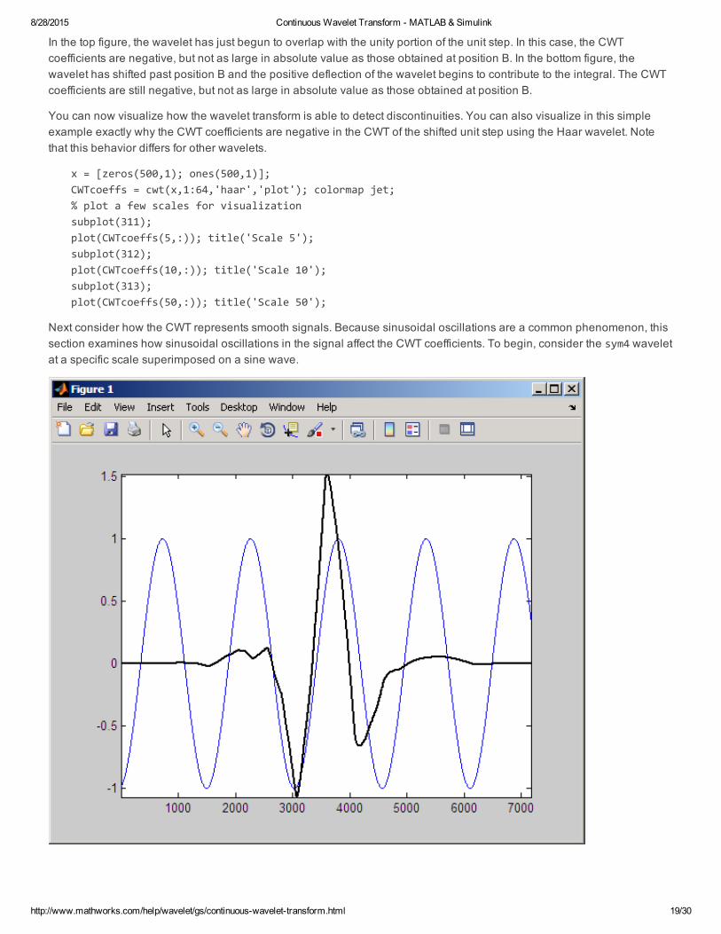
In the top figure, the wavelet has just begun to overlap with the unity portion of the unit step. In this case, the CWTcoefficients are negative, but not as large in absolute value as those obtained at position B. In the bottom figure, thewavelet has shifted past position B and the positive deflection of the wavelet begins to contribute to the integral. The CWTcoefficients are still negative, but not as large in absolute value as those obtained at position B.

You can now visualize how the wavelet transform is able to detect discontinuities. You can also visualize in this simpleexample exactly why the CWT coefficients are negative in the CWT of the shifted unit step using the Haar wavelet. Notethat this behavior differs for other wavelets.

x = [zeros(500,1); ones(500,1)];CWTcoeffs = cwt(x,1:64,'haar','plot'); colormap jet;% plot a few scales for visualizationsubplot(311);plot(CWTcoeffs(5,:)); title('Scale 5');subplot(312);plot(CWTcoeffs(10,:)); title('Scale 10');subplot(313);plot(CWTcoeffs(50,:)); title('Scale 50');

Next consider how the CWT represents smooth signals. Because sinusoidal oscillations are a common phenomenon, thissection examines how sinusoidal oscillations in the signal affect the CWT coefficients. To begin, consider the sym4 waveletat a specific scale superimposed on a sine wave.



Recall that the CWT coefficients are obtained by computing the product of the signal with the shifted and scaled analyzingwavelet and integrating the result. The following figure shows the product of the wavelet and the sinusoid from thepreceding figure.

You can see that integrating over this product produces a positive CWT coefficient. That results because the oscillation inthe wavelet approximately matches a period of the sine wave. The wavelet is in phase with the sine wave. The negativedeflections of the wavelet approximately match the negative deflections of the sine wave. The same is true of the positivedeflections of both the wavelet and sinusoid.

The following figure shifts the wavelet 1/2 of the period of the sine wave.



Examine the product of the shifted wavelet and the sinusoid.



You can see that integrating over this product produces a negative CWT coefficient. That results because the wavelet is 1/2cycle out of phase with the sine wave. The negative deflections of the wavelet approximately match the positive deflectionsof the sine wave. The positive deflections of the wavelet approximately match the negative deflections of the sinusoid.

Finally, shift the wavelet approximately one quarter cycle of the sine wave.



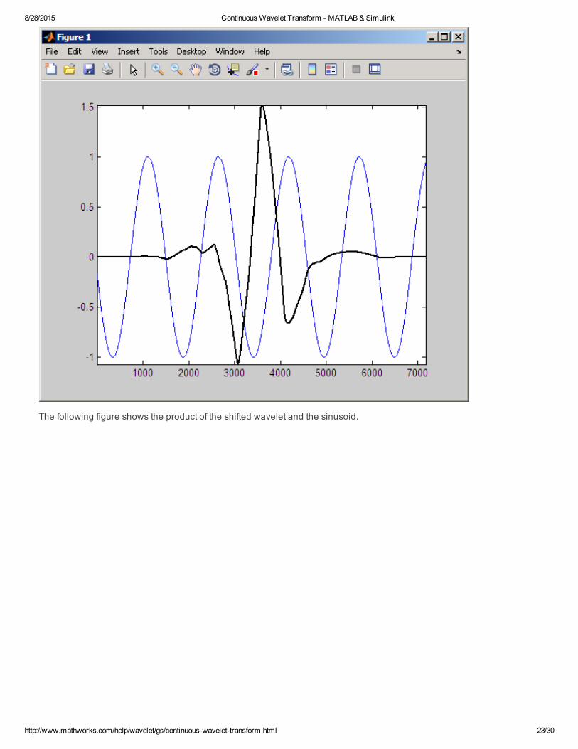
The following figure shows the product of the shifted wavelet and the sinusoid.



Integrating over this product produces a CWT coefficient much smaller in absolute value than either of the two previousexamples. That results because the negative deflection of the wavelet approximately aligns with a positive deflection of thesine wave. Also, the main positive deflection of the wavelet approximately aligns with a positive deflection of the sine wave.The resulting product looks much more like a wavelet than the other two products. If it looked exactly like a wavelet, theintegral would be zero.

At scales where the oscillation in the wavelet occurs on either a much larger or smaller scale than the period of the sinewave, you obtain CWT coefficients near zero. The following figure illustrates the case where the wavelet oscillates on amuch smaller scale than the sinusoid.



The product shown in the bottom pane closely resembles the analyzing wavelet. Integrating this product results in a CWTcoefficient near zero.

The following example constructs a 60Hz sine wave and obtains the CWT using the sym8 wavelet.

t = linspace(0,1,1000);x = cos(2*pi*60*t);CWTcoeffs = cwt(x,1:64,'sym8','plot'); colormap jet;



Note that the CWT coefficients are large in absolute value around scales 9 to 21. You can find the pseudofrequenciescorresponding to these scales using the command:

freq = scal2frq(9:21,'sym8',1/1000);

Note that the CWT coefficients are large at scales near the frequency of the sine wave. You can clearly see the sinusoidalpattern in the CWT coefficients at these scales with the following code.

surf(CWTcoeffs); colormap jet;shading('interp'); view(‐60,12);



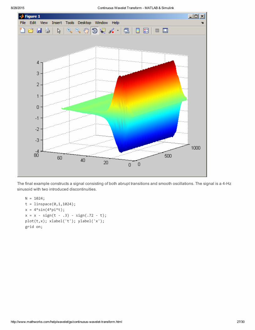
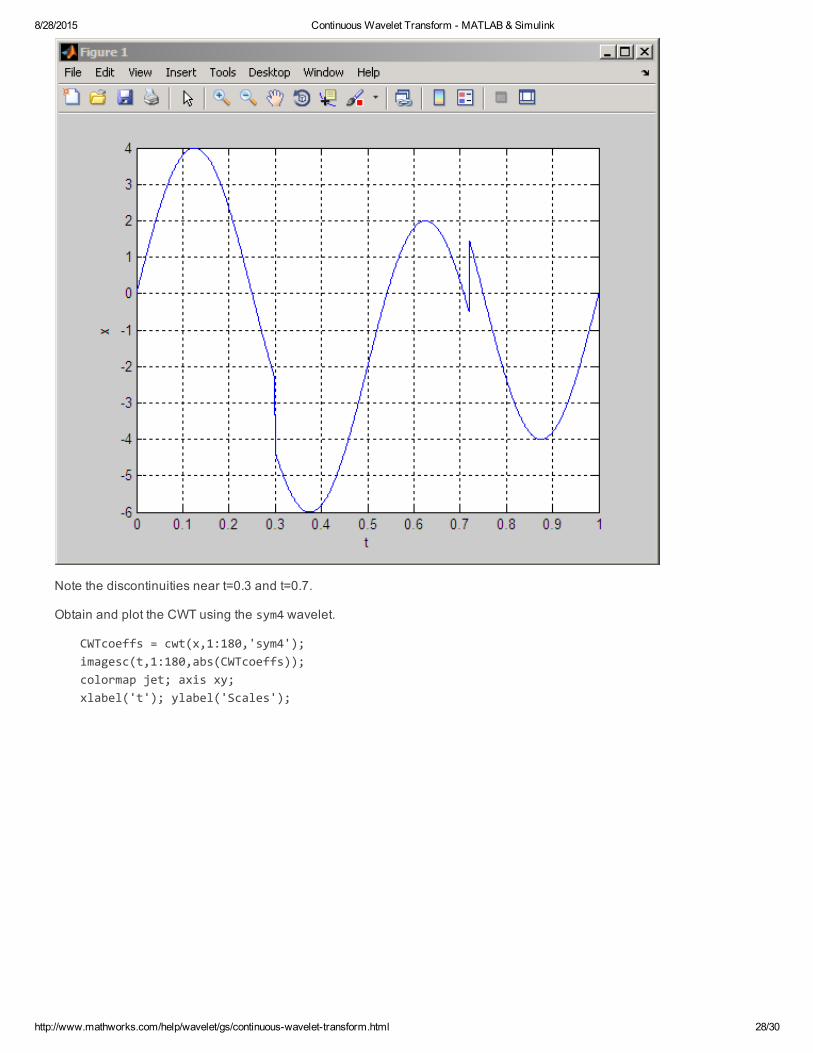
The final example constructs a signal consisting of both abrupt transitions and smooth oscillations. The signal is a 4Hzsinusoid with two introduced discontinuities.

N = 1024;t = linspace(0,1,1024);x = 4*sin(4*pi*t);x = x ‐ sign(t ‐ .3) ‐ sign(.72 ‐ t);plot(t,x); xlabel('t'); ylabel('x');grid on;



Note the discontinuities near t=0.3 and t=0.7.

Obtain and plot the CWT using the sym4 wavelet.

CWTcoeffs = cwt(x,1:180,'sym4');imagesc(t,1:180,abs(CWTcoeffs)); colormap jet; axis xy;xlabel('t'); ylabel('Scales');



•

•

•

Note that the CWT detects both the abrupt transitions and oscillations in the signal. The abrupt transitions affect the CWTcoefficients at all scales and clearly separate themselves from smoother signal features at small scales. On the other hand,the maxima and minima of the 2–Hz sinusoid are evident in the CWT coefficients at large scales and not apparent at smallscales.

The following general principles are important to keep in mind when interpreting CWT coefficients.

Cone of influence— Depending on the scale, the CWT coefficient at a point can be affected by signal values at pointsfar removed. You have to take into account the support of the wavelet at specific scales. Use conofinf to determine thecone of influence. Not all wavelets are equal in their support. For example, the Haar wavelet has smaller support at allscales than the sym4 wavelet.

Detecting abrupt transitions— Wavelets are very useful for detecting abrupt changes in a signal. Abrupt changes in asignal produce relatively large wavelet coefficients (in absolute value) centered around the discontinuity at all scales.Because of the support of the wavelet, the set of CWT coefficients affected by the singularity increases with increasingscale. Recall this is the definition of the cone of influence. The most precise localization of the discontinuity based onthe CWT coefficients is obtained at the smallest scales.

Detecting smooth signal features— Smooth signal features produce relatively large wavelet coefficients at scaleswhere the oscillation in the wavelet correlates best with the signal feature. For sinusoidal oscillations, the CWTcoefficients display an oscillatory pattern at scales where the oscillation in the wavelet approximates the period of thesine wave.

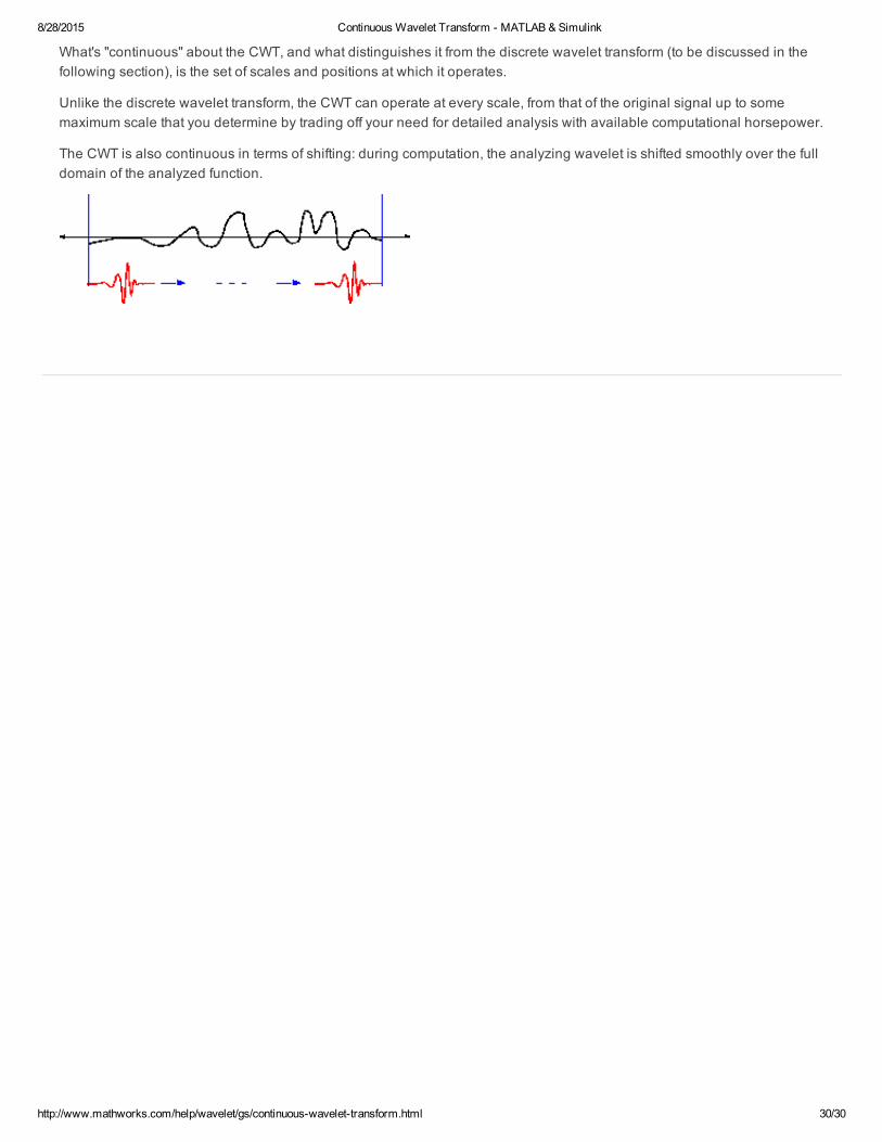
Redundancy in the Continuous Wavelet TransformAny signal processing performed on a computer using realworld data must be performed on a discrete signal — that is, ona signal that has been measured at discrete time. So what exactly is "continuous" about the CWT?

http://www.mathworks.com/help/wavelet/ref/conofinf.html



What's "continuous" about the CWT, and what distinguishes it from the discrete wavelet transform (to be discussed in thefollowing section), is the set of scales and positions at which it operates.

Unlike the discrete wavelet transform, the CWT can operate at every scale, from that of the original signal up to somemaximum scale that you determine by trading off your need for detailed analysis with available computational horsepower.

The CWT is also continuous in terms of shifting: during computation, the analyzing wavelet is shifted smoothly over the fulldomain of the analyzed function.

continuous wavelet transform matlab & simulink

Documents