Final chapter for `Recent Developments in Biologically Inspired Computing’, Leandro Nunes de Castro & Fernando J. Von Zuben ( eds.)

Oct.23, 2003

Continuous Attractor Neural Networks Thomas P. Trappenberg Faculty of Computer Science Dalhousie University 6050 University Avenue Halifax, Nova Scotia Canada B3H 1W5 tt@cs.dal.ca Phone: +902-494-3087 Fax: +902-429-1517 Keywords from list http://www.idea-group.com/assets/keywords.asp Neural Networks Cybernetics Additional Keywords: Computational Neuroscience Machine Learning Memory (short term memory, working memory) Attractor Networks Recurrent Networks Network Dynamics Biographical Sketch: Dr. Trappenberg is an associate professor in Computer Science and the director of the electronic commerce program at Dalhousie University, Canada. He received a doctoral degree in natural science in theoretical high energy physics from Aachen University in Germany, before moving to Canada as postdoctoral fellow. Dr. Trappenberg worked for several years in the IT industry before moving to Japan as researcher in the RIKEN Brain Science Institute and becoming the computational neuroscientist at the Centre for Cognitive Neuroscience at Oxford University, England. His research interests are computational neuroscience and data mining, and he is the author of Fundamentals in Computational Neuroscience published by Oxford University Press, 2002.

1

CONTINUOUS ATTRACTOR NEURAL NETWORKS Abstract In this chapter a brief review is given of computational systems that are motivated by information processing in the brain, an area that is often called `neurocomputing’ or `artificial neural networks’. While this is now a well studied and documented area, specific emphasis is given to a subclass of such models, called continuous attractor neural networks, which are beginning to emerge in a wide context of biologically inspired computing. The frequent appearance of such models in biologically motivated studies of brain functions gives some indication that this model might capture important information processing mechanisms used in the brain, either directly or indirectly. Most of this chapter is dedicated to an introduction to this basic model and some extensions that might be important for their application, either as model of brain processing, or in technical applications. Direct technical applications are only emerging slowly, but some examples of promising directions are highlighted in this chapter. INTRODUCTION Computer Science was, from its early days, strongly influenced by the desire to build intelligent machines, and a close look at human information processing was always a source of inspiration. Walter Pitts and Warren McCulloch published a paper in 1943 entitled `A Logical Calculus of Ideas Immanent in Nervous Activity’, in which they formulated a basic processing element that resembled basic properties of neurons that are thought to be essential for information processing in the brain (McCulloch & Pitts, 1943). Such nodes, or similar nodes resembling more detailed neuronal models, can be assembled into networks. Several decades of neural network research have shown that such specific networks are able to perform complex computational tasks. An early example of biologically inspired computation with neural networks is some work by Frank Rosenblatt and colleagues in the late 1950s and early 1960s (Rosenblatt, 1962). They showed that a specific version of an artificial neural network, which they termed perceptron, is able to translate visual representations of letters (such as the signal coming from a digital camera) into signals representing their meaning (such as the ASCII representation of a letter). Their machine was one of the first implementations of an optical character recognition solution. Mappings between different representations are common requirements of advanced computer applications such as natural language processing, event recognition systems, or robotics. Much of the research and development in artificial neural networks has focused on perceptrons and their generalization, so called multilayer perceptrons. Multilayer perceptrons have been shown to be universal approximators in the sense that given enough nodes and the right choice of parameters, such as the individual strength of

2

connection between different nodes, multilayer perceptrons can approximate any function arbitrarily close (Hornik et al., 1989). Much progress has been made in the development and understanding of algorithms that can find appropriate values for the strength of connections in multilayer perceptrons based on examples given to the system. Such algorithms are generally known as (supervised) learning or training algorithms. The most prominent example of a training algorithm for multilayer preceptrons, which is highly important for practical applications of such networks, is the error-backpropagation algorithm that was widely popularized in the late 1980s and early 1990s (Rumelhart et al., 1986). Many useful extensions to this basic algorithm have been made over the years (see for example Watrous, 1987; Neal, 1992, Amari, 1998), and multilayer-perceptrons in the form of back-propagation networks are now standard tools in computer science. Multi-layer perceptrons, which are characterized by strict feed-forward processing, can be contrasted with networks that have feedback connections. A conceptually important class of such networks has been studied considerably since the seventies (Grossberg, 1973; Wilson & Cowan , 1973; Hopfield, 1982; Cohen & Grossberg, 1983). Systems with feedback connections are dynamical systems that can be difficult to understand in a systematic way. Indeed, systems with positive feedback are typically avoided in engineering solutions, as they are known to create the potential for systems which are difficult to control. The networks studied in this chapter are typically trained with associative learning rules. Associative learning, which seems to be a key factor in the organization and functionality of the brain, can be based on local neural activity, which was already suggested in 1948 by Donald Hebb in his famous and influential book `The Organization of Behavior’ (Hebb, 1948). The locality of the learning rules are useful also in artificial systems as they allow efficient implementation and parallelization of such information processing systems. Recurrent networks of associative nodes have attractive features that can solve a variety of computational tasks. For example, these networks have been proposed as a model of associative memory, where the memory states correspond to the point attractors in these dynamical systems that are imprinted by Hebbian learning. These type of recurrent networks are therefore frequently called (point) attractor neural networks (ANNs). The associative memory implemented by such networks has interesting features such as the ability to recognize previously stored pattern from partial input, a high degree of fault tolerance with respect to a partial loss of the network, and the efficiency of learning from single examples; all features that are of major interest to computer scientists. Another closely related class of recurrent network models have a specifically organized connectivity structure and are now commonly termed continuous attractor neural network (CANN) models. Such models have been studied in conjunction with many diverse brain functions including local cortical processing (Hansel & Sampolinski, 1998), saccadic motor programming (Kopecz & Schöner, 1995), working memory (Compte et al., 2000; Wang, 2001), and spatial representation (Skaggs et al, 1995; Redish et al, 1996; Zhang, 1996). The diversity of application of this model in computational neuroscience indicates that related mechanisms are used widely in the information processing in the brain. In this chapter we outline some of the features of such networks and only start to

3

explore how these mechanisms can be used in technical applications. Some examples of basic operations implemented by such networks are briefly outlined, specifically the implementation of an arg max function through cooperation and competition in such networks, and the maximum likelihood decoding of distributed information representations. COMPUTATIONAL NEUROSCIENCE AND BIOLOGICALLY FAITHFUL MODELING While artificial neural networks, especially in the form of backpropagation networks, have been developed into useful engineering tools, they have been developed in a direction that is not strictly biologically plausible. This is acceptable in technical applications that do not have to claim biological relations. However, the study of biologically plausible information processing has important aspects that should not be forgotten. This includes the desire to understand how the brain works, which will, for example, enable the development of new treatment methods for brain deceases. The experimental knowledge of brain functions has increased tremendously over the last several decades, and has particularly accelerated recently after the arrival of powerful new brain imaging techniques such as functional Magneto Resonance Imaging (fMRI) and advanced single cell recording methods. Such methods advanced considerably our understanding of where and how information is represented in neuronal activity, and the scientific area of computational neuroscience seeks to understand how the processing of such information is achieved in the brain. Of course, modeling of complex systems such as the brain has to be done on multiple levels. Indeed, the art of scientific explanations is to find the right level of abstraction rather than the detailed reproduction of nature. It can be questioned if rebuilding a complete brain in silicon would advance our knowledge; I would argue that this would mainly demonstrate the state of our knowledge. In contrast, finding the right level of description can considerably enhance our understanding and technical abilities. A good example is the advent of thermodynamics that describe large particle systems on a macroscopic level, by Ludwig Boltzmann and J Willard Gibbs in the late 19th century. Surely, a gas is a system of weakly interacting particles, but their macroscopic description has advanced our technical abilities considerably. Modeling of brain functions has to be viewed in a similar way. Some models are abstract representations of high level mental processes, while other models describe the detailed biophysics of neurons. Backpropagation networks have made head-waves in cognitive science as useful metaphors of cognitive processes (Parallel Distributed Processing). It does, however, become questionable that such learning algorithms describe metal processes on a level of networks of neurons. Although some attempts have been made to justify their biological plausibility (see for example O’Reilley & Munakata, 2000), several questions remain when it comes to the biological justification of such networks on a neuronal level. This does not only include the learning rule itself, which requires the

4

questionable backpropagation of error signal through the network, but also includes other constrains on network architectures, including the typical drastic constraint on the number of hidden nodes in multilayer feedforward networks required to facilitate generalization in such networks. While the brain might still use information processing along the lines of mapping networks, networks that translate a distributed representation of some kind into another, it seems that the majority of cortical processing is based on different principles of network operations, including diverging-converging chains (Abeles, 1991) and Hebbian-type learning (Hebb, 1949). A well recognized fact of brain networks, which is conceptually very different to multilayer perceptrons, is that there is an abundance of reciprocal connections between brain areas that defy the strict layered architecture of perceptrons. While the role of feedback connections between distinct brain areas is still under investigation with regards to the system-level implementation of information processing in the brain, some progress has been made in understanding local organizations of brain networks that exhibit local (collateral) feedback connections (see for example Grossberg & Williamson, 2001). A prime example of this is the processing in the CA3 area of the hippocampus (Rolls & Treves, 1998). The models described in this chapter fall in the category of network level models that can be related to brain networks comprised of a few cubic millimeters of brain tissue with internal recurrent connections. THE BASIC PROCESSING ELEMENT The basic processing element in the networks described here is called a node to remind ourselves that these are typically only rough approximations of biological neurons. The term artificial neuron is also commonly used to label such processing elements, although it has been argued extensively in recent years that such nodes, most commonly used in neural network computing, are better interpreted as describing the average behavior of a population of neurons (Wilson & Cowan, 1973, Gerstner 2000). A basic node is illustrated in Figure 1A. This node receives input values on each of its input channels, and each of the input values is then multiplied by the weight value associated with the respective input channel. The node then sums all the weighted input values and generates an output based on a gain function g(x), where the argument of this function is the sum of the weighted input values. The gain function thus describes the specific activation characteristics of the node. Some examples of frequently used gain function are summarized in the table shown in Figure 1B. This simple node is only a very rough abstraction of a biological neuron. A schematic example of a biological neuron is illustrated in Figure 1C. The analogy of these processing elements stems from the basic facts that a neuron can receive input signals from different neurons through the release of chemical at the end of the sending neurons. These chemicals, called neurotransmitters, can produce a change in the potential of the receiving neuron. The strength of the generated potential change can thereby vary for different input channels. Changes of the electrical potential from different sources simply

5

add to each other, so that the neuron is in its simplest abstraction basically summing all the weighted inputs. An output signal, which typically takes the form of an electrical impulse called a spike, is generated by the neuron if the potential change generated by all the inputs in a certain time window reaches some threshold. The generated spike can then trigger the release of neurotransmitters at the sending ends of this neuron.

igure 1: A. Basic node in a neural network that represents population activity. B. Examples of gain

any of the biochemical mechanisms of the information transduction of a neuron

Ffunctions frequently used in technical applications of artificial neural network. C. Schematic outline of a biological neuron.

Moutlined above are known in much more detail and can be incorporated in more detailed models of neurons (Hodgkin & Huxley, 1952; FitzHugh, 1961; Nagumo et al., 1962; Connor & Stevens, 1971; Wilson, 1999). Indeed, models of spiking neurons (see Maass and Bishop, 1998, for some general introduction), that have been first introduced in the early 20th century (Lapicque, 1907), are becoming increasingly incorporated in detailed models of brain tissue. However, many of the information processing principles in the brain, specifically on a larger system level that comprises many thousand of neurons, are often studied with networks of nodes that represent average firing rates of neurons. Indeed, it can be shown that a node of the type illustrated in Figure 1A can properly represent the average response of a collection of neurons with similar response properties if various conditions are fulfilled, including slow varying changes in the population and the absence of spike synchronization effects (Gerstner, 2000). The basic message here is that the population averages of neuronal responses of brain tissue can be modeled to some degree with simple processing elements as illustrated in Figure 1A, and that it is possible that many different forms of gain functions can be realized by small neuronal

6

networks. We could study the specific realization of specific nodes in biological terms in more detail, but we choose here to move forward in the direction of exploring the computational consequences of specific networks of such simple nodes. FEED-FORWARD VERSUS RECURRENT NETWORKS

s mentioned in the introduction, a very popular organization of nodes into networks is

nother network organization of simple nodes, which is the focus of this chapter, is

Athe layered structure as outlined in Figure 2A. Such networks operate in a strictly feedforward manner, in which each node in each layer receives inputs from the previous layers and generate outputs that are used in the subsequent layers. An input pattern fed to such a network can take the form of a vector with one component for each of the input nodes. The output can be represented as a vector with the number of components equal to the number of output nodes. With this formulation of the system a feedforward network can be seen as implementing a mapping function from one vector space into another. As mentioned above, a multilayer perceptron can in principle realize any mapping between two vector spaces with the proper assignment of parameters (Hornik et al., 1989). Finding the appropriate parameters in order to realize a specific mapping function is the task of a learning algorithm, of which the error-backpropagation algorithm is the most prominent example for such networks. This algorithm is based on the maximization of an objective function (or minimization of an energy function) with a gradient-ascent (or gradient-descent) method. Many training samples are typically required to discover the statistical structure of the underlying mapping function.

Figure 2: Two principal network architecture used frequently in neural network computing, that of a multilayer perceptron (A) and a recurrent network (B).

Aillustrated in Figure 2B. There is only one layer in this network architecture, and the output of this layer is fed back as input to the network in addition to potential external

7

input such networks can receive. Thus, even with a constant input, the state of the network can change within each execution step as the effective input of the network might change over time. Such a network is a dynamical system, and it turns out that the behavior of this system depends strongly on the values of the connection weight parameters. There are many possible choices of weight values, and we will meet two procedures in this chapter to choose specific values, either setting these parameters in an organized way according to a predefined function, or using a learning procedure to adapt these parameters based on examples shown to the network. The learning algorithms typically used with such network architectures are so called

ecurrent networks trained on random patterns with a Hebbian learning rule have

OINT ATTRACTOR VERSUS CONTINUOUS ATTRACTOR

nother way in which the basic recurrent networks discussed here are used to model

Hebbian rules, which are learning algorithms that change the weight values according to the state (activity) of the nodes that frame a specific connection (the link between the nodes). Such rules are local because the change in the connection strength depends only on information firing in the framing nodes of each link. The network activity during the learning phase is kept clamped to constant values supplied by the external input. The recurrent connections have therefore no effect during this learning phase. This is important as the recurrent connections could otherwise modify the node values in complex ways and thereby destroy the information that we seek to store in such networks. Note that the resulting weight values in Hebbian rules will ultimately be symmetric in the sense that a connection from node a to node b will have the same value as a connection from node b to node a. Rinteresting properties when it comes to a retrieval phase after learning. In such a phase the network is initialized with a possible noisy version of one of the training patterns that was used during learning. During the updating of the network the state of the network evolves with each update-iteration, until the network reaches a point where the node activities do not change any more. Such a state is a point attractor in the dynamical system of this recurrent network, and such networks are therefore often called (point) attractor neural networks (ANNs). ANNs are useful devices because the point attractors can correspond to stored pattern in such networks. Thus, stored patterns can be retrieved from partial information (associative memories) or noisy versions of a stored pattern (noise reduction). An example program that demonstrates the associative storage abilities of an ANN network is detailed in APPENDIX A. PNETWORKS Abrain functions are models in which the weight values are pre-assigned with specific values. A common choice in neuroscience is thereby marked by a specific interaction structure, that of local cooperation and global competition. This is implemented with weight values that only depend on the distance between nodes: nodes that are `close’

8

have a positive weight value (excitatory), whereas weight values of mutually `distant’ nodes have negative (inhibitory) weight values. We will discuss below in more detail the meanings `close’ and `distant’ can have, but for now it is sufficient to think of a chain of nodes as illustrated in Figure 2B and to use the Euclidean distance between the nodes as a measure of their closeness.

Figure 3: A. Time evolution of network states in a CANN model; B. Isolated point attractors and

positive weight value between close nodes creates localized positive feedback loops in

ow many different attractor states exist in this network? In networks with perfectly shift invariant interaction structures it is possible to stabilize an activity packet around each

basin of attractions in ANN models; C. A line of point attractors in a CANN model.

Awhich any initial node activity gets reinforced between such nodes. We call such activity an activity packet. The effect of an activity packet on other nodes in the network is that it suppresses other network activity through the long-range inhibition. This balance between local excitation and global inhibition is the source of the formation of an activity packet in the network. An example of the time evolution of the network activity in such a network is shown in Figure 3A. A corresponding example MATLAB program that specifies the details of the model is given in the APPENDIX B. The network was, in the shown experiment, initialized with equal node activity, but an external input centered around the central nodes in the network was applied for the first 10 iterations (time-steps). The strong response in node activity to the external input is clearly visible, but what is most important for our following discussions is that an activity packet persists even after the external input is removed. This activity packet is an attractor state of the network. Any external input that is symmetric around the center of this attractor state will lead to the same asymptotic activity packet after the external input is removed. H

9

node of the network by applying an initial external input centered around the node on which the activity packet should be stored. The number of attractor state does thus scale with the number of nodes in the network. It follows that it is possible to increase the number of attractor states by increasing the density of nodes in the network. Mathematically it is possible to think about a continuum of nodes that represents a neural field. Such a neural field model has then a continuous manifold of point attractors, which motivated the name continuous attractor neural networks (CANNs) for such models. Those networks are still point attractor neural networks but with a specific point attractor structure, that of a continuous manifold of point attractors. Although truly continuous manifolds of point attractors exist only in the limit of an infinite number of nodes, the name CANN is also used for discrete models when the number of nodes is sufficiently large to approximate the continuous case sufficiently. This convention is adopted in the following. The different attractor structures of recurrent networks discussed here are illustrated in

igure 3B and C. The previously discussed associative memory networks have point

RAINING CONTINUOUS NEURAL NETWORKS

with pre-assigned eight vales. A typical example of the weight profiles is a Gaussian function of the

al systems. Such structure can, for example, evolve from the growth of neural structures in a systematic

Fattractors that are surrounded by a basin of attraction. The network state evolves to the point attractor that lies within the basin of attraction in which the network is started. This is why a point attractor structure with separated point attractors is useful as associative memory. A continuous attractor network is not useful as associative memory because perturbations of a network state that are not symmetric to an initial activity packet can trigger different attractor states. However, these networks can still be used as memories in the sense that they can hold information given to the network over a period of time. Such networks are therefore short-term (erasable) memory stores, and there are indications that the brain uses these mechanisms for such purposes (Compte et al., 2000; Wang, 2001). However, there are also several other features of such networks that might not only be utilized in the brain, but might allow the use of such networks in technical applications. Some of the features and possible applications will be explored below. T CANN models in the neuroscience literature are commonly employed wweight values as a function of the Euclidean distance as illustrated in Figure 4. We mentioned above that it is necessary for CANN to have interaction structures with short distance excitation and long-distance inhibition, but we can always absorb the negative values for long distances in a global inhibition constant that shifts the Gaussian toward negative values. We can therefore simplify the following description by outlining the following thoughts with only positive weight values while keeping in mind that a global constant inhibition is part of the network operation (see APPENDIX B). The pre-assigned interaction structure can be well motivated in biologicaway, with short excitatory neurons that project to local neurons, and inhibitory neurons that project to more distant neurons. Cortical organizations are not obviously consistent

10

with this view as inhibitory interneurons are typically short-ranged. However, it is possible that the long-range inhibition is an emerging property of the pool of inhibitory interneurons. It is also possible that the cortex employs the mechanisms discussed in the following only on a local level. The basic CANN model discussed here should be viewed as a simplified model that allows the outline of some general properties of such networks. Nevertheless, some brain areas have been shown to be consistent with an effective interaction structure typical to CANN models. An example is the superior colliculus, a midbrain area that is important in the integration of information to guide saccadic eye movements (Trappenberg et al., 2001, see Figure 4B).

Figure 4: A. Illustration of the connection strength between nodes in a one-dimensional CANN model with Gaussian profile. The solid line represents the connection strength between the center node and

atic euronal interaction structures in the brain, such a pre-assignment is not possible if the

all the other nodes in the network. This node is connected most strongly to itself, followed by the connection to it nearest neighbors. The dotted lines represent the corresponding curves for the other nodes in the network. B. Normalized effective interaction profile in the monkey superior colliculus (see Trappenberg et al., 2001). The data points with different symbols are values derived from different cell recordings, while the solid line is a model fit.

Although there are many biologically plausible mechanisms to assign very systemneffective network architecture has to be able to adapt to changing environments. Adaptive mechanisms of weight values are then mandatory, and training algorithms become central for such applications. An area in the brain that has an unusual number of feedback connections to the same brain area is the CA3 structure in the hippocampus, a brain area that is associated with episodic memories. Episodic memories are memories of specific events as opposed to memories with more generic content such as acquired motor skills. The anatomic organization of this brain structure, as well as many experimental findings from cell recordings, strongly suggests that associative memories of the recurrent network type discussed here might be a mechanism used in this brain area to support episodic memories, and that Hebbian learning could be the principal biological mechanism that supports the adaptation in this brain structure. Indeed, the hippocampus was the area where long-term potentiation (LTP) and long-term depression (LTD), the

11

synaptic expression underlying Hebbian learning in the brain, was first discovered (Bliss & Lomo, 1973). Interestingly, studies of the hippocampus in rodents indicate that this brain structure is

sed to represent spatial information of specific environments in these animals. Neurons

again that the network has to be trained on all attractor states, hich is an infinite number in the case of a true continuous attractor network for a neural

uthat respond in a specific way to the location of an animal have been termed place cells. The physiological properties of place cells have long been modeled with CANNs. However, a topographical structure that relates the physical location of a cell to the feature values it represents with its activity response has not been found. This indicates that if CANN models are the underlying mechanisms of place cells, the systematic interaction structure in CANN models must be able to evolve through learning. As the hippocampus exhibits LTP and LTD it is obvious that Hebbian learning should be able to form the specific interaction structures from specific training examples. Indeed, applying Hebbian learning to all attractor states of a continuous attractor does result in weight values that only depend on the distance of neurons with respect to their response properties (e.g. distance in feature space) with local excitation and global inhibition (Stringer et al., 2002). It is worth highlightingwfield model. The number of attractor states can still be very large in the discrete approximation of such models with a finite number of nodes. However, the training on all possible states is only necessary in a strict mathematical sense. With small modifications of the model, which are outlined in the next section, it is possible to achieve sufficient training with a small fraction of the possible states in the network.

OISE AND TRAINING ON SMALL TRAINING SETS: NMDA TABILIZATION

of attractors in recurrent network models only exists if the weight rofile is shift invariant. This means that the weight values do only depend on the

NS A continuous manifoldpdistance between nodes and not on their index numbers. For example, a weight value between node number 12 and 17 has to be exactly the same as the weight value between node 240 and 245 if the nodes are spaced equidistantly and numbered in sequence. Any small fluctuation of the strict equivalence results in a drift of an activity packet, and the model has then isolated point attractors instead of the continuous manifold of point attractors. An example of the drift of the activity packets is shown in Figure 5A. In this experiment a Gaussian weight function was augmented by noise. The figure displays several lines, each line represents the time evolution of the center of mass of the network activity after initializing the network with an activity packet at a different node in the network. Figure 5B shows an example of a similar experiment where the network was trained on only a subset of all possible states (10 out of 100). No noise was added to the resulting weight values, but the training on the subset of possible training patterns resulted again in an attractor structure with isolated point attractors.

12

Figure 5: Drifting activity packet in a network with noisy connections (A) and partially trained network (B). C. Inclusion of some NMDA stabilization in the partially trained network.

To solve the problem of drifting activity packets in such CANN models, Stringer et al.

001) proposed a modification of the basic CANN model in which the firing threshold is ecreased for the nodes that were active in the previous time step. A possible neuronal

nly a subset of all possible training atterns, an increase of the number of attractor states can be seen (Figure 5C). It is

s mentioned above, the point attractor states in ANN models are useful as associative memory states because they correspond to patterns on which the network was trained,

(2dequivalent of such a mechanism is provided by the voltage dependence of NMDA-mediated ion channels. A NMDA receptor is a specific subclass of a glutamate receptor that can be activated with the pharmacological substance N-methyl-D-aspartic acid (NMDA). Most important for the mechanisms explored here is the characteristic of the associated ion channels that their permeability for ions depends on the postsynaptic potential. When these ion channels are opened by glutamate while the postsynaptic potential is at rest, then the ion channel is blocked by magnesium ions. Depolarization of the membrane removes this blockage so that sodium and potassium ions, as well as a small number of calcium ions, can enter the cell. NMDA synapses are typically co-located with non-NMDA synapses that do not depend on the postsynaptic potential. The net effect of these two channels is thus a lower excitation threshold of the neuron following previous excitation, which is the mechanism implemented in the simulations. We refer to this mechanism as NMDA-stabilization. When including NMDA-stabilization in the computer simulations of the previous experiment, in which the network was trained on oppossible to achieve a different number of attractor states by varying the amount by which the firing threshold is decreased after a node becomes active. However, it is important to adjust this amount carefully to not disrupt the CANN features in this network. LOAD CAPACITY OF ATTRACTOR MODELS A

13

and these memories can be triggered by patterns with some sufficient overlap with the ained patterns. The number of stored patterns P relative to the number of connections

d above, these attractor states are only of limited use with respect associative memory states. Nevertheless, these states are still memory states in the

el (Stringer et al, 2003; Trappenberg 2003). However, activity packets have still be sufficiently distant from each other, for they would otherwise attract each other and

trper node C in the network is called the load α=P/C of the network. It is possible to add attractor states through Hebbian learning in such networks until a critical load αc is reached; at which point all the attractor states related to the stored pattern become unstable. This critical load is also called the load capacity of the network. The load capacity achieved with Hebbian learning on random binary patterns is αc=k/(a log(a)), where k is a constant with value k ≈ 0.2-0.3, and a is the average sparsness of the pattern, which is the ratio of ones to zeros in the case of binary patterns (Rolls & Treves, 1998). The maximal possible load capacity, which can be achieved with an optimal learning rule, is k=2 (Gardner, 1987). We are considering here fully connected networks in which the number of connections per node is equal to the number of nodes in the network. The load capacity of these point attractor networks does therefore scale with the number of nodes in the network. Attractors can be stabilized around each node in CANN models, and the load capacity of CANN models does therefore also scale with the number of nodes in the network. However, as mentionetosense that they keep the information that was given to them by an initial input that subsequently disappeared. This is the basis for using CANN models as short-term memory stores. Hence, rather than counting the number of attractor states in these networks, it is more crucial to ask how many short-term memories can be stored simultaneously in such networks. The answer is one and only one. The competitive nature of network activity in these networks enforces the survival of only one activity packet after external input to the systems is removed, even if the external input has several peaks in the activity distribution. Indeed, this is a major feature of these networks that can be used for specific information processing implementations discussed further below. Before we leave the load capacity issue it is worth mentioning that the number of concurrent activity packets can be increased with the inclusion of NMDA -stabilization in the modtomerge to one activity packet. The possible number of concurrent activity packets does thus depend on the size of the activity packet, which is in turn a function of the width of the weight function. Typical values of such widths, which are consistent with physiological evidence in the brain, allow only a small number of concurrent activity packets in such networks even with the inclusion of stabilization mechanisms along the lines discussed in the previous section. This is a possible explanation of the source of the limited storage capacity of human working memory (Trappenberg, 2003), which is know to be severely limited to a small number such as 7±2 (Miller, 1956).

14

APPLICATIONS OF CANNS: WINNER-TAKES-ALL AND OPULATION DECODING

computational ications that such mechanisms are used frequently for

formation processing in the brain (Wilson & Cowan, 1973; Grossberg, 1973; Amari,

tivity packet, where the position of the activity packet is determined by the upport it gets from the initial input pattern. Through the cooperation between close

. An example can be seen when two initial activity packets ith similar magnitude are supplied as initial input. If such initial activity packets are

et Zhang, 1997; Deneve et al., 1999, 2001; Wu et al., 2002). It is well established that the

P Continuous attractor neural networks are of central importance in neuroscience as there are strong indin1977; Taylor & Alavi, 1995; Compte et al., 2000; Trappenberg et al 2001). The study of CANN models, in general as well as in specific computational circumstances, is important in order to see if such models can explain measured effects, or if, on the contrary, the experimental data indicate that other mechanisms must be at work in the brain. While there are strong beliefs that CANN mechanisms are central for information processing in the brain, the exploration of their potential in technical applications has only begun. A basic feature of CANN models it that an initial distributed input will evolve into stereotyped acsnodes and the competition between distant nodes, locations with the strongest support will win the competition. The support is thereby a combination of the initial activity of single nodes in combination with the activity of neighboring nodes, and the CANN models implement thereby a specific version of a winner-take-all algorithm. This winner-take-all algorithm could be of practical use in many applications. A standard winner-take-all algorithm relies basically on an arg max function that returns the index of the largest component of a vector. This is a global operation and as such computationally inefficient. CANN models offer an interesting version of such functions with the potential of efficient implementations in a distributed system. The utilization of CANN in applications that rely on winner-take-all or winner-take-most algorithms should be explored in further research. Note that CANNs can be even more flexible than functions that look strictly only for the largest component of a vectorwclose to each other, then it is possible that the two activity packets merge under the dynamics of the system into an activity packet somewhere in between the two initial stimuli locations (see Figure 6). This is a form of vector averaging often observed in related psychophysical processes such as rapid saccades made to two close targets. The location of the asymptotic activity packet can be a complicated function of the initial input pattern, and several different solutions are possible with different choices of weights used in specific networks. There are thus many possible applications of such networks in systems that need to implement complicated conflict-resolution strategies. A related interesting application of CANN models, with potential relevance for brain processes and technical applications was recently explored in a variety of papers (Poug&brain represents information, such a sensory input, in a distributed way in the activity of neural responses (see Abbott & Sejnowski, 1999). Many neurons are typically involved

15

in the stimulus representation rather than a single neuron, which is the basis of the distributed nature of information encoding in the brain. Distributed representations have interesting features for technical applications; not only can such system be designed to operate in a more efficient way through parallel processing of chunks of information, but they allow in addition the design of systems which are robust in terms of losing complete information due to partial system errors. The challenge with distributed codes is the decoding of the information, the process of deducing the most likely stimulus given a certain activity pattern of the nodes.

Figure 6: Experiment with two external Gaussian signals that are given to the CANN until t=10. The resulting activity packet after equilibration is an average of the two external locations.

ponses with spect to a feature value conveyed by a stimulus. This function is often called the tuning

with population ode to be decoded. The CANN model is then an implementation of a fitting procedure of

Population decoding can be a computationally expensive task, and the process is certainly simplified if we know the principal form of the function of the node resrecurve of a node. There is however another factor that makes population decoding challenging in the brain, which is the large amount of noise present in the activation of neurons. In other words, there is only a certain probability that a specific stimulus initiates a certain activity of a node. It is hence appropriate and useful to formulate population decoding in statistical terms, and many statistical methods have been devised to solve decoding in noisy environments (see for example Abbott & Sejnowski, 1999). One important method is based on the maximum likelihood estimation. This specific method is equivalent to a least square fit of the tuning curve to the node responses in the case that the conditional activation probabilities are Gaussian functions. The use of CANN models for population decoding is based on the idea that a specific form of an activity packet will appear after initializing such networks ca function, which is given by the shape of the attractor states, to data, which are given as initial states to the network. Tuning curves of neurons in the brain often appear to be approximately Gaussian-shaped, and the asymptotic activity packets in CANN models

16

can have a similar form. Indeed, the attractor states can be made exactly Gaussian with a proper normalization of the weight values in the training procedure (Deneve et al., 1999). Thus, CANN models can be an efficient implementation of maximum likelihood decoding of distributed codes (Wu et al., 2002). A simplified example is shown in Figure 7. A Gaussian signal (dashed line) was thereby convoluted with additive white noise, which resulted in the noisy signal shown as dotted

ne in the figure. This signal was given to a CANN as initial stimulus, and the network liwas allowed for several time steps to evolve after the initial input was removed. The resulting activity packet (solid curve) resembles closely the initial noiseless signal.

Figure 7: Illustration of the application of CANN for noisy population decoding. The original signal (dashed line) is convoluted with additive white noise. This noisy input signal (dotted line) is given to a CANN network as initial state. Resulting firing pattern of the network is shown s solid line, which

TIONS FROM DIFFERENTIAL FORMATION: PATH-INTEGRATION

e hippocampus

in the environment. Such models are o used in a similar way to model cells that represent head directions of the rodents.

aresembles closely the original signal.

UPDATING REPRESENTAIN

As mentioned above, CANN models are used to model place fields in thof rodents that represent the location of the animalalsSuch cells are a good example of how the state of an animal, in this case spatial information, is represented internally in the brain. Of course, such external representations have to be updated when the position of the animal changes. This can be achieved efficiently by external stimuli such as the sight of a specific landmark in the environment. In the CANN model, this corresponds to a new external input to the network that would trigger the corresponding attractor state.

17

However, it is also well known that internal spatial representations, such as the sense of location or direction, can be updated in the dark where visual cues cannot be used. Self-

enerated (idiothetic) cues have therefore to be the source of updating the states of

of the basic model that result in an effectively asymmetric weight function. was mentioned above that the symmetry of the weight function is required to enable

gCANN models. An obvious source of such information is the vestibular system, which is based on motion sensors in the ears. Such idiothetic information does not represent absolute geographic coordinates but rather the change of positions or orientations in time. Hence, there must be a mechanism to integrate this information with the absolute positioning information represented by place or head direction cells. This mechanism was termed path-integration in the area of place representation, and the term is now often used generically for updating absolute representations from signals representing differential information. The basic idea of enabling path-integration in CANN models is based on a specific modification Itstable, non-shifting activity packets. Asymmetric weight functions support one kind of neighboring nodes more than others, which results in a shift of the activity packet. The basic method of enabling path-integration in CANN models is hence to modulate the asymmetry of a basic symmetric weighting function. This can be achieved through predefined, specifically organized networks (Skaggs et al., 1995), but it is also possible to achieve such organizations through learning procedures in CANN models (Zhang, 1996; Stringer et al., 2002).

Figure 8: A. Outline of the network architecture to enable path-integration in CANN models. B. Effective weights between CANN nodes without input from the rotation nodes (solid line) and with

18

input from the clockwise rotation node (dashed line). C. Evolution of an activity packet in the path-integration network. A clockwise rotation node is activated at time t=20τ, which drives the activity packet towards positive node numbers until the rotation node activity is rest to zero. A counter -clockwise rotation node is then activated more strongly at t=50τ, which increases the velocity of the reverse movement.

The key ingredient in the path-integration algorithm for CANN networks is the addition of connections from cells that have activity related to the motion information. In the case of a head direction system they are called rotation nodes. Activities in the rotation nodes have the effect of modulating the recurrent connections in the CANN model. The modified network architecture is illustrated in Figure 8A. Only connections between neighboring nodes in the recurrent network, and the corresponding connections between rotation nodes and the CANN nodes, are shown for simplicity. The connections between the rotation nodes and the CANN nodes can be trained with Hebbian learning based on the co-activation between the rotation nodes and the CANN nodes. An example of resulting weight values is shown in Figure 8B. The solid line represents the symmetric excitatory weights between CANN nodes if none of the rotation nodes are active. The effective weights between the CANN nodes for some activity of the clockwise nodes are shown as a dotted line. This asymmetric nature of these weights drives the activity packet in a clockwise direction. An example of the resulting network activity is shown on Figure 8C. The network isinitialized after training, with an external input at node number 50 and no activity in the

city. The movement of the activity packet stops as soon as the activity the rotation node is withdrawn. Stimulation of the counter-clockwise rotation node

world of technical applications. Examples are robot navigation and speech generation, and many other areas of applications can be explored.

rotation nodes. After withdraw of the external input the network maintains the location of the activity packet through the baseline connections in the network that are symmetric. An external activation in the clockwise rotation node is then introduced at time t=20τ. This results in an effective asymmetric weight profile between CANN nodes, which in turn results in a movement of the activity packet towards higher node numbers with constant veloofresults in a movement of the activity packet in the opposite direction. The velocity of the movement depends thereby on the activity strength of the rotation node. The activity of the counter-clockwise rotation node was set to twice the value in the clockwise movement in the specific example shown in Figure 8C. This resulted in an increased movement velocity of the activity packet in the reverse direction. Path-integration can be realized in different, more direct ways on computer systems, and it is obvious to ask how such a network implementation of an integration algorithm could be useful in technical applications. It is, of course, crucial to have such an algorithm if we want to update feature values that are represented in CANNs, with all their advantages of distributed systems in terms of fault tolerance and computational efficiency. However, in addition to these obvious advantages it is also interesting to note that the above path-integration algorithm is adaptive, as the weight values are learned from specific examples (Stringer et al., 2002). Such systems can hence be used to learn motor sequences, which

pen the doors to a wholeo

19

Neuroscientific research indicates that nature does use such mechanisms in the brain, but more research into the specific advantages and applications of such networks is required. HIGHER-DIMENSIONAL MODELS Most of the discussions in this chapter have been made exemplary for one-dimensional CANN models that can store one continuous feature value (or attribute) through the location of an activity packet. However, all the mentioned features of CANN models can be generalized to higher-dimensional CANN models. Instead of a line of nodes, leading to a line of point attractors, a two-dimensional sheet of neurons with corresponding weight structure gives rise to a two-dimensional sheet of point attractors, and higher-dimensional arrangements of nodes can be used to realize higher-dimensional attractor manifolds. Predefined weight structures are only one way to

realize such attractor odels, and we stressed in this chapter that a training algorithm with specific training

at the effective model is high dimensional just based on the number of nodes that are ost strongly connected. At some point we might want to choose appropriate definitions

e the principal idea without giving ecific numbers.

shown with line widths that are proportional to the weight strength. No rganized structure can be found in this example. However, in Figure 9C the nodes are

reorganized so that nodes with strong connections are plotted close to each other, and

msets can be used to set up this weight structure. This opens the door to an interesting application of such networks in the discovery of the association structure of the underlying problem, in particular, the effective dimensionality of data used to train the networks. Recurrent networks, in which every node is connected to all the nodes in the network, can be viewed as a high-dimensional model if we take the number of neighbors as the defining characteristic of the dimensionality. For example, each node in a chain of nodes with Gaussian weight profiles has two distinguished neighbors if we take only the strongest connections into account. A two dimensional grid of nodes with the corresponding two-dimensional Gaussian weight profile has 4 neighbors. If we set the weight values before learning to equal numbers for all connections, than we could say thmfor dimensionality, but for now it is sufficient to outlinsp The dimensionality discovery ability of the Hebbian-trained recurrent networks is outlined with an example shown in Figure 9. There we choose a network of 20 nodes that are arbitrarily numbered and arranged in a circle. The initial equal connection strength between the nodes is illustrated with connecting lines of equal width in Figure 9A. Each node was given randomly one of the directions for which it would respond most vigorously (random preferred directions). The learning phase consisted of presenting Gaussian activity profiles for all possible direction to the network. That is, for each pattern the nodes were clamped to a value that decayed according to a Gaussian function with respect to the distance of the preferred direction of this node with the direction represented by the training pattern. The resulting weight values of the connections after training on these training data are shown in Figure 9B, where only the strongest weight values are o

20

nodes with weaker connections are plotted more remotely. The resulting structure is one dimensional, reflecting the structure of the training space. If the activation of the nodes during training had been caused by a two-dimensional training set structure, then there would be connections between the nodes outside the one-dimensional arrangement of nodes, and a two dimensional re-arrangement of nodes would have to be performed to find an orderly organization of the connections proportional to their strength values. Even without realizing the arrangement it is possible to use some form of appropriate counting of nodes with similar weight values as an indicator of the dimensionality of the underlying feature space.

Figure 9: A. Fully connected network of 20 nodes before training when all connections have the same weight. B. The network after training, where the weight strength is indicated with the line-width of the connections. C. Network after training when the nodes are arranged so that neighboring nodes have strong weights (see also Trappenberg, 2002).

Note that this procedure is complementary to a self-organizing map (SOM) as proposed, for example, by Kohonen (1994). The dimensionality of SOM model is predefined by the dimensionality of the SOM grid. This can be viewed as a predefined lateral (recurrent) interactions structure. Indeed, a major step in SOM algorithms is to find the node that is most activated by a specific training stimulus (winner-takes-most), and this step can be viewed as a shortcut to a possible neural implementation based on CANN models. The major difference between the SOM model and CANN model is that the SOM model

ains the receptive fields (input connections) to the recurrent networks based on a fixed interaction structure in the SOM layer, whereas the trained CANN model adapts the interaction structure within the recurrent network with fixed receptive fields. An interesting class of models known as neural gas models (Matinetz & Schulten, 1991) are set up to train both type of connections. However, this is only useful if different timescales of the adaptation time for the different type of connections are used. SUMMARY AND OUTLOOK Continuous attractor neural networks have been discussed in the neuroscience related literature for nearly 30 years, and it is increasingly evident that such mechanisms are used

tr

21

in the brain. Such mechanisms must therefore be useful for information processing in distributed systems. Continuous attractor networks implement cooperation and competition between input stimuli, and the network dynamics drive initial input to one of many attractor states based on some dominating input features. Such networks can be used to resolve competition in various ways. This is closely related to winner-take-all mechanisms, but such networks can certainly implement more complicated versions of such mechanisms than only looking for the largest component in a vector. The recently explored application of CANNs for population decoding is a good example. CANNs represent thereby efficient implementations of a maximum likelihood estimator, and similar applications of such algorithms are likely to emerge. More research into theapplication of such networks in related problem domains could be a fruitful endeavor.

ANNs have a strict regularity of the connection weights that defines the network, which

patterns as mentioned in the text, which should be explored further. This is, of course, losely related to associative learning, and it is good to stress again the close relation of

s solve specific computational problems.

EFERENCES

Ccan often be set according to a function so that there is no need for lengthy training algorithms. However, it is also possible to use Hebbian learning to define the weights. A possible application of such training is the discovery of the relation structure of training

cCANN networks to the more commonly known ANN (attractor or Grossberg-Hopfield neural networks). Many additions to the basic CANN model have been proposed in recent years that are destined for further explorations into various application areas. Among these additions is an elegant way of updating the memory in such networks from differential information, commonly known as path-integration. Such mechanisms have many potential applications in motor control and navigation, as is evident form their possible role in related biological systems. It is possible to train such networks on specific examples and thus implement memories of specific movement patterns. Many applications of such mechanisms are possible, and such mechanisms might be at work in the brain, for example in the acquisition of motor primitives. Further research is necessary to explore these possibilities and to establish more specific algorithms based on CANN mechanismto R Amari S. (1977). Dynamics of pattern formation in lateral inhibition type neural field. Biological Cybernetic 27, 77-87. Amari S. (1998). Natural gradient works efficiently in learning. Neural Computation 10, 251-276. Abbott, L. & Sejnowski, T.J. (eds.) (1999). Neural Codes and Distributed Representations: Foundations of Neural Computation (Cambridge, MA, MIT Press)

22

Abeles, M. (1991). Corticonics: neural circuits of the cerebral cortex (Cambridge, Cambridge University Press). Bliss, T. V. P. & Lomo, T. (1973). Long-lasting potentation of synaptic transmission in the dendate area of anaesthetized rabbit following stimulation of the perforant path. Journal of Physiology 232, 551-556. Cohen, M.A. & Grossberg, S. (1883). Absolute stability of global pattern formation and parallel memory storage by competitive neural networks}, IEEE Trans. on Systems, Man and Cybernetics SMC-13, 815-26. Compte, A., Brunel, N., Goldman-Rakic, P.S. & Wang, XJ. (2000). Synaptic mechanisms

e Neuroscience 2, 740-745.

eneve S., Latham, P.E. & Pouget, A. (2001). Efficient computation and cue integration n codes. Nature Neuroscience 4, 826-831.

, 445-466.

481-485.

Studies in Applied Mathematics 52, 217-257.

ebral Cortex 11, 37-58.

e, MA, MIT Press).

and network dynamics underlying spatial working memory in a cortical network model. Cerebral Cortex 10, 910-23. Connor, J.A. & Stevens, C.F. (1971). Prediction of repetitive firing behaviour from voltage clamp data on an isolated neuron soma. Journal of Physiology 213, 31-53. Deneve S., Pouget A. & Latham, P.E. (1999). Divisive Normalization, Line Attractor Networks and Ideal Observers. Advances in Neural Information Processing Systems 11. Deneve S., Latham, P.E. & Pouget, A. (1999). Reading population codes: a neural implementation of the ideal observer, Natur Dwith noisy populatio FitzHugh, R. (1961). Impulses and physiological states in theoretical models of nerve membranes. Biophysics Journal 1 Gardner, E. (1987). Maximum storage capacity in Neural Networks. Electrophysics Letters 4, Gerstner, W. (2000). Population Dynamics of Spiking Neurons: Fast Transients, Asynchronous States, and Locking. Neural Computation 12, 43-89. Grossberg, S. (1973). Contour enhancement, short-term memory, and constancies in reverberating neural networks, Grossberg, S. & Williamson, J.R. (2001). A neural model of how horizontal and interlaminar connections of visual cortex develop into adult circuits that carry out perceptual groupings and learning. Cer Hansel, D. & Sampolinsky, H. (1998) .Modeling feature selectivity in local cortical circuits. In Koch, C. & Segev, I (eds), Methods in neural modeling: From Ions to networks, second edition (Cambridg

23

Hebb, D. O. (1949). The Organization of Behavior: A neuropsychological theory (New York, Wiley). Hodgkin, A.L. & Huxley, A.F. (1952). A quantitative description of membrane current

,

9, 2554-8.

d networks are niversal approximators. Neural Networks 2, 359-366.

ntegrating visual formation and pre-information on neural, dynamic fields. Biological Cybernetics

ohonen, T. (1984). Self-Organization and Associative Memory (Berlin, Springer-

apicque, L. (1907). Recherches quantitatives sur l’excitation electrique des nerfs traitee 5.

aass, W. & Bishop, C.M. (eds.) (1998). Pulsed Neural Networks. (Cambridge, MA,

artinetz, T.M. & Schulten, K.J. (1991). A neural-gas network learns topologies. etworks

cCulloch, W. & Pitts, W. (1943). A logical calculus of the ideas immanent in nervous

minus two: Some limits on our apacity for processing information. Psychological Review 63, 81-97.

rimoto, S. & Yoshizawa, S. (1962). An active pulse transmission line imulating nerve axon. Proc IRE 50, 2061-2070.

od, Report CRG-TR-92-1, University of Toronto, Toronto, Canada.

O’Reilly, R.C. & Munakata, Y. (2000). Computational Exploration in Cognititve Neuroscience (Cambridge, MA, MIT Press)

and its application to conduction and excitation in nerves. Journal of Physiology, 117500-544. Hopfield, J.J. (1982) Neural networks and physical systems with emergent collective emergent computational abilities. Proceeding of the National Academy of Science PNAS 7 Hornik, K., Stinchcombe, M. & White, H. (1989). Multilayer feedforwaru Kopecz, K. & Schöner, G. (1995). Saccadic motor planning by iin73, 49-60. KVerlag). Lcomme une polarization. Journal de Physiologie et Pathologie Général 9, 620-63 MMIT Press). MIn Kohonen, T., Mäkisara, K., Simula, O., &. Kangas, J. (eds), Artificial Neural N(Amsterdam, North-Holland). Mactivity. Bulletin of Mathematical Biophysics 5, 115-133. Miller, G.A. (1956). The magical number seven, plus or c Nagumo, J.S., As Neal R.M. (1992). Bayesian training of backpropagation networks by the hybrid MonteCarlo meth

24

Pouget, A. & Zhang, K. (1997). Statistically Efficient Estimations Using Cortical Lateral Connections. In Mozer, M.C., Jordan, M.I., Petsche, T. (eds), Advances in Neural

formation Processing Systems 9, 97.

8). Statistically Efficient stimation Using Population Coding. Neural Computation 10, 373-401.

t on system, Network: Computation in Neural Systems 7, 671—685.

ford Press).

umelhart, D. E., Hinton, G. E. & Williams, R. J. (1986). Learning

kaggs, W.E., Knierim, J.J., Kudrimoti, H.S. & McNaughton, B.L. (1995). A Model of een,

tringer, S.M., Trappenberg, T.P., Rolls, E.T. & Araujo, I.E.T. (2002). Self-organising

, 217-242.

, 161-182.

itted

ls in itive Neuroscience 13, 256-271.

radient neural

etworks, M. Caudill and C. Butler (eds.), Vol. 2, 619-627, New York, IEEE.

In Pouget, A., Zhang, K., Deneve, S. & Latham, P.E. (199E Redish, A., Elga, A. & Touretzky, D. (1996). A coupled attractor model of the rodenhead directi Rolls, E. T. & Treves, A. (1998). Neural Networks and Brain Function (Oxford, OxUniversity Rosenblatt, F. (1962). Principles of Neurodynamics (Spartan, New York).

Rrepresentations by back-propagating errors. Nature 323, 533--536.

Sthe Neural Basis of the Rat's Sense of Direction. In Tesauro, G., Touretzky, D., & LT. (eds.), Advances in Neural Information Processing Systems 7, 173-180. Scontinuous attractor networks and path integration: One-dimensional models of head direction cells. Network: Computation in Neural Systems 13 Stringer S.M., Rolls E.T., Trappenberg T.P. & de Araujo I.E.T. (2003). Self-organizing continuous attractor networks and motor function. Neural Networks 16 Taylor, J.G. & Alavi, F.N. (1995). A global competitive neural network. Biological Cybernetics 72, 233-248. Trappenberg, T.P. (2002). Fundamentals of computational neuroscience (Oxford, OxfordUniversity Press). Trappenberg, T.P. (2003). Why is our capacity of working memory so large? Submto Neurocomputing: Letters & Reviews. Trappenberg, T.P, Dorris, M., Klein, R.M, & Munoz, D.P. (2001). A Model of saccade initiation based on the competitive integration of exogenous and endogenous signathe superior colliculus. Journal of Cogn Watrous, R.L. (1987). Learning algorithms for connectionist networks: Applied gmethods of nonlinear optimization. IEEE first international conference inn

25

Wang, X.-J. (2001). Synaptic reverberation underlying mnemonic persistent activity.

rends in Neuroscience 24, 455-463.

wan, J. D. (1973). A mathematical theory of the functional dynamics f cortical and thalamic nervous tissue, Kybernetik 13, 55-80.

Wilson, H.R. (1999). Simplified dynamics of human and mammalian neocortical

Wu, S., Amari, S. & Nakahara H. (2002). Population coding and decoding in a neural

mics of head-irection cell ensembles: a theory. Journal of Neuroscience 16, 2112-2126.

T Wilson, H. R. & Coo

neurons. Journal of Theoretical Biology 200, 375-88.

field: a computational study. Neural Computation 14, 999-1026. Zhang, K. (1996). Representation of spatial orientation by the intrinsic dynad

26

APPENDIX A: A MATLAB IMPLEMENTATION OF AN ATTRACTNEURAL NETWORK SIMULATION

OR

d a fy the details of such

etworks. The aim of this section is to run a simple computer experiment that

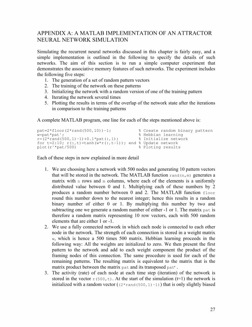
1. The generation of a set of random pattern vectors 2. The training of the network on these patterns 3. Initializing the network with a random version of one of the training pattern 4. Iterating the network several times 5. Plotting the results in terms of the overlap of the network state after the iterations

in comparison to the training patterns

A complete MATLAB program, one line for each of the steps mentioned above is: pat=2*floor(2*rand(500,10))-1; % Create random binary pattern w=pat*pat'; % Hebbian learning r=(2*rand(500,1)-1)+0.1*pat(:,1); % Initialize network for t=2:10; r(:,t)=tanh(w*r(:,t-1)); end % Update network plot(r'*pat/500) % Ploting results Each of these steps in now explained in more detail

1. We are choosing here a network with 500 nodes and generating 10 pattern vectors that will be stored in the network. The MATLAB function rand(n,m) generates a matrix with n rows and m columns, where each of the elements is a uniformly distributed value between 0 and 1. Multiplying each of these numbers by 2 produces a random number between 0 and 2. The MATLAB function floor round this number down to the nearest integer; hence this results in a random binary number of either 0 or 1. By multiplying this number by two and subtracting one we generate a random number of either -1 or 1. The matrix pat is therefore a random matrix representing 10 row vectors, each with 500 random elements that are either 1 or -1.

2. We use a fully connected network in which each node is connected to each other node in the network. The strength of each connection is stored in a weight matrix w, which is hence a 500 times 500 matrix. Hebbian learning proceeds in the following way: All the weights are initialized to zero. We then present the first pattern to the network and add to each weight component the product of the framing nodes of this connection. The same procedure is used for each of the remaining patterns. The resulting matrix is equivalent to the matrix that is the matrix product between the matrix pat and its transposed pat’.

3. The activity (rate) of each node at each time step (iteration) of the network is stored in the vector r(500,t). At the start of the simulation (t=1) the network is initialized with a random vector ((2*rand(500,1)-1)) that is only slightly biased

Simulating the recurrent neural networks discussed in this chapter is fairly easy, ansimple implementation is outlined in the following to specindemonstrates the associative memory features of such networks. The experiment includesthe following five steps:

27

with the first training pattern (0.1*pat(:,1)). The starting state of the network ishence a random version of one of the ar

bitrarily chosen training pattern.

4. The state of the nodes is then updated for nine additional time steps. In each time

e the development of evolution of the network states we plot the at we used during training. We

t between the state of the network r

A r

step we calculate the new state of a node by first summing the weighted inputs to this node from all the other nodes (w*r(:,t-1)). The new state value of the node is then given by the hyperbolic tangent of this value, where tanh is the specific choice of the transfer function used in this simulation.

5. Finally, to examinoverlap of the network state with all the patterns ththereby defined the overlap as the dot producand each training pattern r'*pat/500.

esulting plot of running the program is shown in Figure 10.

0: Results from an ANN simulation. Each of the 10 lines in the plot correspond to the overlap

distance) between the network state at each time step (abscissa) and a pattern that was used arning phase for training. The network state has initially only a small overlap with all of the atterns, but one of the stored patterns was retrieved completely at time step 9. This is an with a rather long convergence time

Figure 1(cosine in the lestored pexample . Many other examples have much smaller convergence tim

es.

28

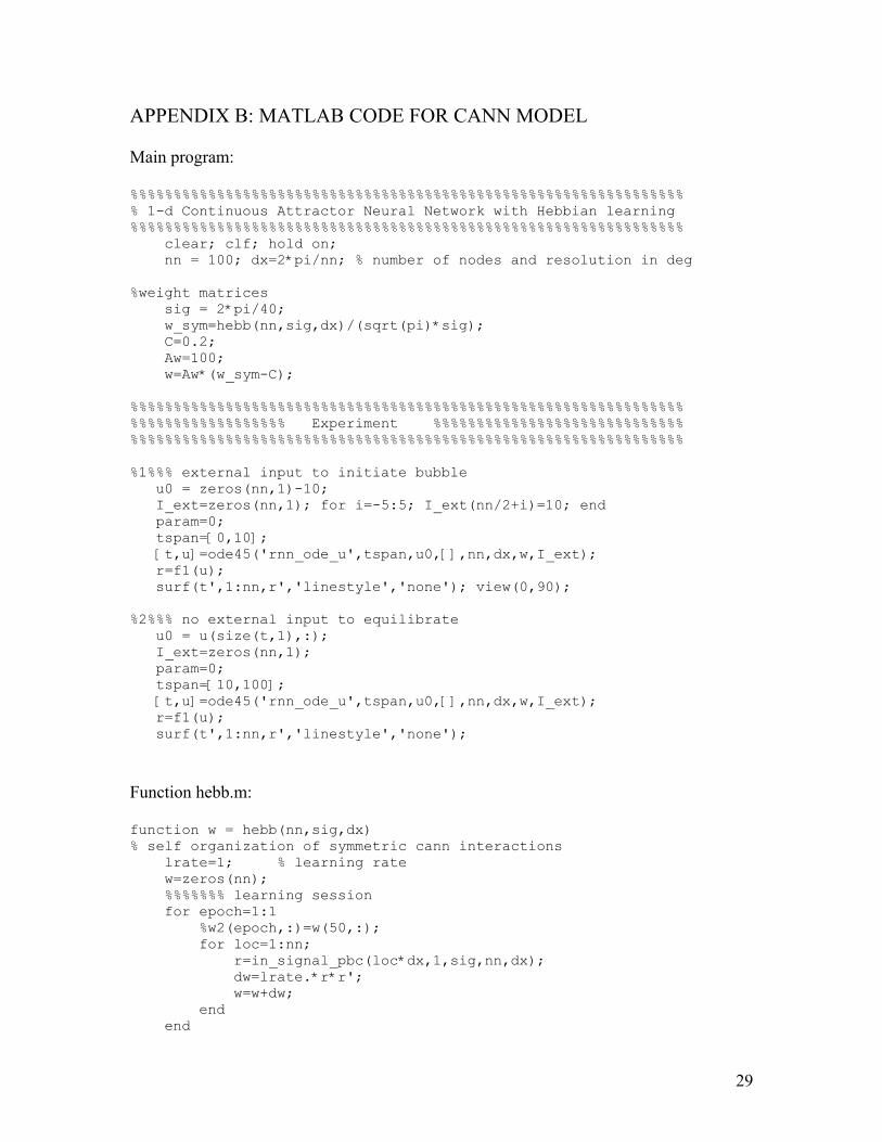
APPE Ma %%%%%%% 1-d %%%%%%%%%%%%%%%%%%%%%%%%%%%%%%%%%%%%%%%%%%%%%%%%%%%%%%%%%%%%%%%% %weigh si w_sym=hebb(nn,sig,dx)/(sqrt(pi)*sig);

w=Aw*(w_sym-C); %%%%%%%%%%%%%%%%%%%%%%%%%%%%%%%%%%%%%%%%%%%%%%%%%%%%%%%%%%%%%%%% %%%%%%%%%%%%%%%%%% Experiment %%%%%%%%%%%%%%%%%%%%%%%%%%%%% %%%%%%%%%%%%%%%%%%%%%%%%%%%%%%%%%%%%%%%%%%%%%%%%%%%%%%%%%%%%%%%% %1%%% external input to initiate bubble u0 = zeros(nn,1)-10; I_ext=zeros(nn,1); for i=-5:5; I_ext(nn/2+i)=10; end param=0; tspan=[0,10]; [t,u]=ode45('rnn_ode_u',tspan,u0,[],nn,dx,w,I_ext); r=f1(u); surf(t',1:nn,r','linestyle','none'); view(0,90); %2%%% no external input to equilibrate u0 = u(size(t,1),:); I_ext=zeros(nn,1); param=0; tspan=[10,100];

hebb.m:

function w = hebb(nn,sig,dx) % self organization of symmetric cann interactions lrate=1; % learning rate w=zeros(nn); %%%%%%% learning session for epoch=1:1 %w2(epoch,:)=w(50,:); for loc=1:nn; r=in_signal_pbc(loc*dx,1,sig,nn,dx); dw=lrate.*r*r'; w=w+dw; end end

NDIX B: MATLAB CODE FOR CANN MODEL

in program:

%%%%%%%%%%%%%%%%%%%%%%%%%%%%%%%%%%%%%%%%%%%%%%%%%%%%%%%%%% Continuous Attractor Neural Network with Hebbian learning

clear; clf; hold on; nn = 100; dx=2*pi/nn; % number of nodes and resolution in deg

t matrices g = 2*pi/40;

C=0.2; Aw=100;

[t,u]=ode45('rnn_ode_u',tspan,u0,[],nn,dx,w,I_ext); r=f1(u); surf(t',1:nn,r','linestyle','none'); Function

29

w=w*dx; return

unction rnn_ode_u.m:

t; sum+I_ext);

F function udot=rnn(t,u,flag,nn,dx,w,I_ext)

etwork % odefile for recurrent n tau_inv = 1./1; % inverse of membrane time constant

=f1(u); r sum=w*r*dx+I_ex udot=tau_inv*(-u+return

:

dx-loc));

nction f1=rnn(u)

(u-alpha)));

Function in_signal_pbc.m function y = in_signal_pbc(loc,ampl,sig,nn,dx) y=zeros(nn,1); for i=1:nn; di=min(abs(i*dx-loc),2*pi-abs(i*

di^2/(2*sig^2)); y(i)=ampl*exp(- end return

Function f1.m: fu% gain function: logistic beta =.1; alpha=.0; f1=1./(1+exp(-beta.*return

30