electronics

Article

Context-Aware Link Embedding with Reachabilityand Flow Centrality Analysis for Accurate SpeedPrediction for Large-Scale Traffic Networks

Chanjae Lee 1 and Young Yoon 2,3,*1 Department of Artificial Intelligence, Big Data, Hongik University, 94 Wausan-ro, Sangsu-dong, Mapo-gu,

Seoul 04068, Korea; arisel117@gmail.com2 Department of Computer Engineering, Hongik University, 94 Wausan-ro, Sangsu-dong, Mapo-gu,

Seoul 04068, Korea3 Neouly Incorporated, 94 Wausan-ro, Sangsu-dong, Mapo-gu, Seoul 04068, Korea* Correspondence: young.yoon@hongik.ac.kr; Tel.:+82-2-320-1659

Received: 26 September 2020; Accepted: 28 October 2020; Published: 29 October 2020�����������������

Abstract: This paper presents a novel method for predicting the traffic speed of the links on large-scaletraffic networks. We first analyze how traffic flows in and out of every link through the lowest costreachable paths. We aggregate the traffic flow conditions of the links on every hop of the inbound andoutbound reachable paths to represent the traffic flow dynamics. We compute a new measure calledtraffic flow centrality (i.e., the Z value) for every link to capture the inherently complex mechanismof the traffic links influencing each other in terms of traffic speed. We combine the features regardingthe traffic flow centrality with the external conditions around the links, such as climate and time ofday information. We model how these features change over time with recurrent neural networks andinfer traffic speed at the subsequent time windows. Our feature representation of the traffic flow forevery link remains invariant even when the traffic network changes. Furthermore, we can handletraffic networks with thousands of links. The experiments with the traffic networks in the Seoulmetropolitan area in South Korea reveal that our unique ways of embedding the comprehensivespatio-temporal features of links outperform existing solutions.

Keywords: link embedding; traffic speed prediction; traffic flow centrality; reachability analysis;spatio-temporal data; artificial neural network; deep learning; context-awareness

1. Introduction

Accurate prediction of speed on traffic networks helps improve traffic management strategiesand generate efficient routing plans. However, precisely estimating the traffic speed in advance hasbeen a non-trivial task since various factors determine traffic flows in many ways.

Various approaches have been used for traffic speed prediction using statistical methods [1–7]and machine learning with neural networks with deep hidden layers [8–18]. However, the existingsolutions are mostly limited to estimating traffic speed for either a single road link or a small-scalesub-network with only a handful of traffic links (e.g., a crossroad). In reality, a road system is alarge-scale connected graph with the traffic links affecting each other’s traffic flow over time in amore complicated fashion that cannot be explained easily with a simple statistical model. The workswithout a broader view of the traffic links may not adequately unravel the hidden, but critical speedprediction factors.

In this paper, we adapt the node embedding techniques introduced by Hamilton et al. [19].We represent the relationship between links with a feature vector whose size is invariant even whencertain changes are made to the traffic networks’ structure, such as the addition or deletion of roads.

Electronics 2020, 9, 1800; doi:10.3390/electronics9111800 www.mdpi.com/journal/electronics

Electronics 2020, 9, 1800 2 of 16

We analyze how the traffic flows in and out of a link through reachable multi-hop paths computedwith the Floyd–Warshall algorithm [20]. How the links impact each other given the traffic flow analysisis quantified through a novel metric we refer to as Traffic Flow Centrality (TFC). We combine the datarelated to TFC with the external conditions around each link, such as climate and time information(e.g., time of day, the indication of holidays). We use a recurrent neural network algorithm to correlatebetween the composite feature’s temporal transition and the traffic speed of each link. Our methodcaptures the traffic flow dynamics through sub-networks around every link without embeddingthe entire adjacency matrix. Therefore, our method is much more space efficient, and it can handlelarge-scale traffic networks with thousands of links. We also do not face the problem of consideringirrelevant information such as the hollow points around traffic networks when they are representedeither with a sparse adjacency matrix or raster graphics [10,18]. Our solution assesses the impact of theremote links in addition to the adjacent neighbors on traffic flows. Hence, with the broader contextualview and the exclusion of unnecessary information, we expect to outperform the works that basedtheir speed prediction only on the limited view of adjacent links.

This paper is structured as follows: In Section 2, we first review the related work. In Section 3,we introduce the method for inferring traffic speed given the temporal transitions of links’ compositecontextual features that are modeled with a novel link embedding technique. In Section 4, we benchmarkthe performance of our approach against existing works, and we conclude in Section 5.

2. Related Works

In this section, we put our work in the context of various related research works on traffic speedprediction. Recently, artificial neural networks with deep hidden layers have gained popularity,as they are effective at modeling the non-linear traffic speed dynamics. Some of the notable workshave employed FNNs (Fuzzy Neural Networks) [8,9], DNNs (Deep Neural Networks) [11,21],RNNs (Recurrent Neural Networks) [13,14], DBNs (Deep Belief Networks) [12,15], and the IBCM-DL(Improved Bayesian Combination Model with Deep Learning) [17] models. These works have shownmore accurate speed prediction than the approaches that are based on classic statistical methodssuch as ARIMA (Auto-Regressive Integrated Moving Average) models [1–3], SVR (Support VectorRegression) [4,5], and K-NN (K-Nearest Neighbor) [6,7].

When the models are obtained by learning the pattern on a single specific link [1–3,13–15,17],the distinct features of other links may not be adequately accounted for. Thus, modeling the trafficspeed pattern per individual link was discussed in [22]. Nonetheless, the work by Kim et al. [22] stilldid not reflect the substructure of the traffic network around each link.

The works presented in [10,16,23,24] extracted spatial features from a visual representation oftraffic networks. In particular, Zheng et al. [23] used a two-dimensional traffic flow that is embeddedin Convolutional Neural Networks (CNN). They also used a Long Short-term Memory (LSTM) [25]algorithm to model long-term historical data. Similarly, Du et al. [16] represented the passenger flowsamong different traffic lines in a transportation network into multi-channel matrices with deep irregularconvolutional networks. Guo et al. [10] analyzed the congestion propagation patterns based on thetraffic observations recorded at fixed intervals in time and fixed locations in space. They representedthe traffic observation in raster data. Then, all the raster data were fed into a 3D convolutional neuralnetwork to model the spatial information. They used a 3 × 3 convolutional kernel that includes thehollow points where no road lies and no traffic flows. The hollow points in the convolutional kernelmay accidentally reflect stale traffic flows. Instead, Du et al. [16] used an irregular convolution kernelthat refers to the traffic flow values from the adjacent traffic lines to fill in the values of the hollow points.These methods commonly exploit the CNN architecture that effectively models visual imagery [26–28].Furthermore, a family of RNN algorithms such as GRU [29] and LSTM [25] was used so that repetitivetemporal patterns can be discovered. However, these works did not capture the relation between theflow points on the two-dimensional spaces such as junctions, crossroads, and overpasses. Therefore,these models are susceptible to errors by correlating between irrelevant traffic flows. For instance,

Electronics 2020, 9, 1800 3 of 16

they may confuse overpasses and overlapping roads as crossroads. Furthermore, these works did notaddress the impact of the external conditions on the traffic flow. Learning the correlation betweentraffic flows and weather parameters was useful for flow prediction, as presented in [12,30]. However,they overlooked the impact of the substructure around traffic links on traffic flows.

More recently, modeling the traffic flow based on the graph representation of the traffic networkshas emerged. The works presented in [18,31–33] combined GNNs (Graph Neural Networks) [34,35]and RNNs to capture the temporal flow transition patterns given adjacency matrices that explicitlyreflect the complex interconnections. These methods do not have to unnecessarily deal with theinformation irrelevant to the traffic flow, such as the hollow points in the visual traffic networks thatDu et al. [16] had to consider forcefully.

ST-TrafficNet [33] used Caltrans PeMS (Performance Measurement System) data from around20 links between intersection points and predicted traffic speed with stacked LSTM using aspatially-aware multi-diffusion convolution block. This PeMS data were from 350 loop detectorsat 5 min intervals from 1 January 2017 to 31 May 2017. This model reflects spatial influence throughmulti-diffusion convolution with forward, backward, and attentive channels.

TGC-LSTM was used by Cui et al. [18] to predict the traffic speed on four connected freewaysin the Greater Seattle Area. They used publicly available traffic state data from 323 sensor stationsover the entirety of 2015 at 5 min intervals. With their model, traffic speed was predicted with theRMSE (Root Mean Squared Error) as low as 2.1. However, the GNN architecture has to be restructuredwhenever the traffic networks undergo some changes. This is because TGC-LSTM uses the entireadjacency matrix as an input to the GNN instead of embedding the features of individual traffic links.Upon any change to the traffic networks, we have to re-train from scratch with the newly updatedGNN architecture. Furthermore, since TGC-LSTM uses a very large adjacency matrix, both the timeand space complexity of modeling the network structure becomes high. However, more importantly,the larger the adjacency matrix is, the more sparse it becomes. Therefore, TGC-LSTM still faces theproblem of incorporating unnecessary data such as the hollow points captured in a regular convolutionkernel, as discussed in [10]. The shortcomings of these GNN-based approaches motivated us to devisea new method for embedding the characteristics of the traffic network.

We adapt the node embedding techniques introduced by Hamilton et al. [19]. We represent therelationship between links on the traffic network with a feature vector whose size is invariant evenwhen any part of the network structure changes. We analyze how the traffic routes through a linkvia reachable lowest cost multi-hop paths that are computed with the Floyd–Warshall algorithm [20].We compute every link’s relative impact on other links based on its inbound/outbound traffic flowpatterns and its neighbors’ collective conditions. We refer to the relative cross-link impact value asTraffic Flow Centrality (TFC). We combine the features related to TFC with the external conditionsaround each link, such as climate and time information. We use a recurrent neural network algorithmto learn how such a composite feature change over time determines the traffic speed of each link.

Our method does not involve the process of embedding the entire adjacency matrix. Therefore,our solution is more space efficient and can easily handle large-scale traffic networks with thousandsof links. Furthermore, it avoids incorporating irrelevant information such as the hollow pointsthat can be present in traffic networks when they are represented with a sparse adjacency matrixor raster graphics [10,18]. Our solution considers the conditions of the remote links beyond theadjacent neighbors. By ruling out irrelevant information and having the broader contextual view,we expect to outperform the works that base their speed prediction myopically on the conditions ofthe adjacent links.

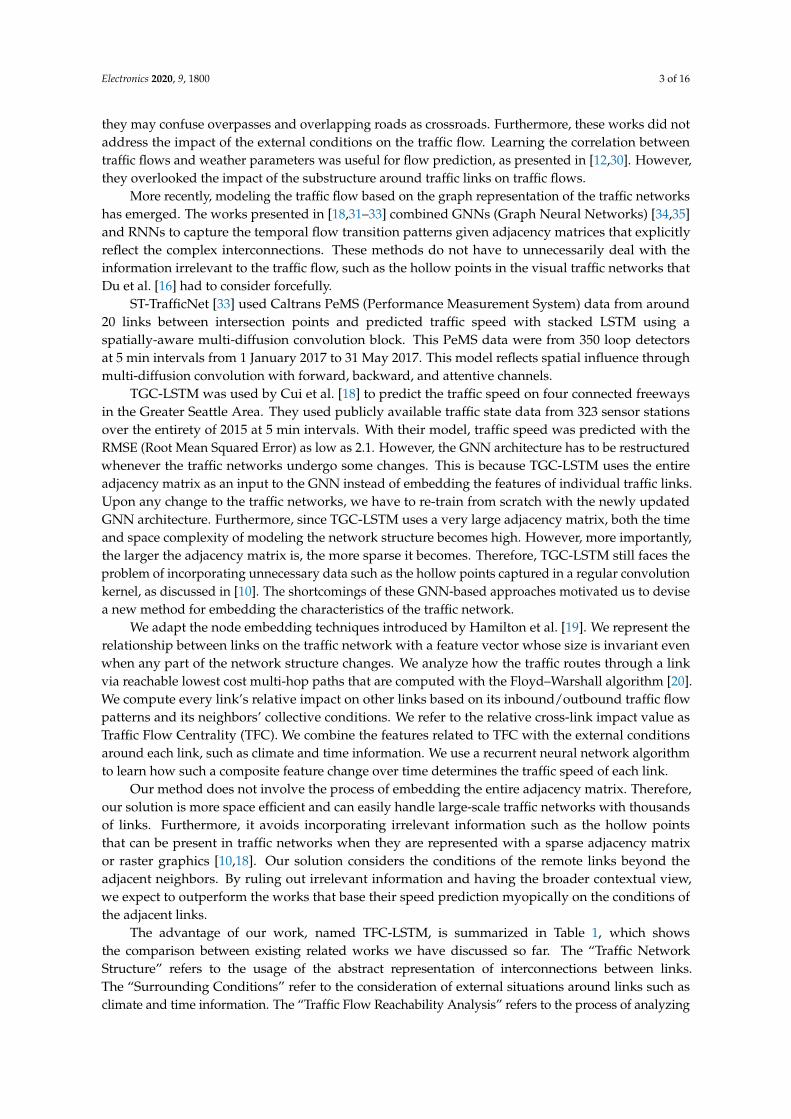
The advantage of our work, named TFC-LSTM, is summarized in Table 1, which showsthe comparison between existing related works we have discussed so far. The “Traffic NetworkStructure” refers to the usage of the abstract representation of interconnections between links.The “Surrounding Conditions” refer to the consideration of external situations around links such asclimate and time information. The “Traffic Flow Reachability Analysis” refers to the process of analyzing

Electronics 2020, 9, 1800 4 of 16

the pattern of traffic flowing in and out of links through reachable paths. The “Centrality Analysis”refers to the usage of the link’s relative influence on others. The “Chains of Neighbors” column indicatesthe consideration of remote neighbors besides the adjacent ones when capturing the substructure arounda link.

Table 1. Comparison with other models. TFC, Traffic Flow Centrality.

Prediction Models

Raw Data Usage Traffic Network Representation

TrafficSpeed/Volume

TrafficNetworkStructure

SurroundingConditions

InvariantInput Feature

Vector Size

Traffic FlowReachability

Analysis

CentralityAnalysis

Chains ofNeighbors

TFC-LSTM O O O O O O O

TGC-LSTM [18] O O X X X X X

ST-3DNET [10] O O X X X X X

DST-ICRL [16] O O O X X X X

IBCM-DL [17] O X X X X X X

DBN [15] O X X X X X X

LSTM [13] O X X X X X X

GRU [14] O X X X X X X

DNN [12,22] O X O X X X X

FNN [8,9] O O X X X O X

K-NN [6,7] O O X X O X X

SVR [4,5] O O X X X X X

ARIMA [1–3] O X X X X X X

“X” means yes, and “O” means no.

3. Methodology

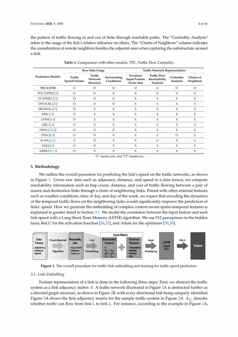
We outline the overall procedure for predicting the link’s speed on the traffic networks, as shownin Figure 1. Given raw data such as adjacency, distance, and speed in a data tensor, we computereachability information such as hop count, distance, and cost of traffic flowing between a pair ofsource and destination links through a chain of neighboring links. Paired with other external featuressuch as weather conditions, time of day, and day of the week, we expect that encoding the dynamicsof the temporal traffic flows on the neighboring links would significantly improve the prediction oflinks’ speed. How we generate the embedding of complex context-aware spatio-temporal features isexplained in greater detail in Section 3.1. We model the correlation between the input feature and eachlink speed with a Long Short-Term Memory (LSTM) algorithm. We use 512 perceptrons in the hiddenlayer, ReLU for the activation function [36,37], and Adam for the optimizer [38,39].

Figure 1. The overall procedure for traffic link embedding and training for traffic speed prediction.

3.1. Link Embedding

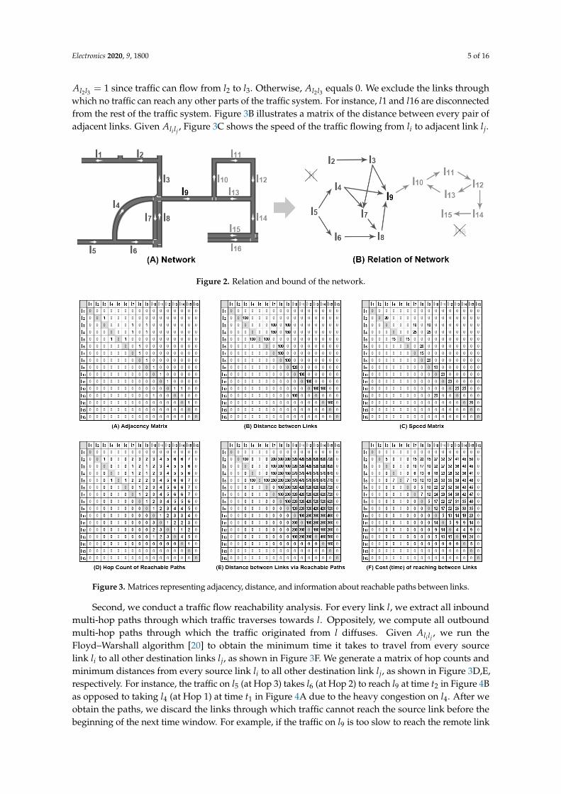
Feature representation of a link is done in the following three steps: First, we abstract the trafficsystem as a link adjacency matrix A. A traffic network illustrated in Figure 2A is abstracted further asa directed graph structure, as shown in Figure 2B, with every directional link being uniquely identified.Figure 3A shows the link adjacency matrix for the sample traffic system in Figure 2A. Ali lj

denoteswhether traffic can flow from link li to link lj. For instance, according to the example in Figure 2A,

Electronics 2020, 9, 1800 5 of 16

Al2l3 = 1 since traffic can flow from l2 to l3. Otherwise, Al2l3 equals 0. We exclude the links throughwhich no traffic can reach any other parts of the traffic system. For instance, l1 and l16 are disconnectedfrom the rest of the traffic system. Figure 3B illustrates a matrix of the distance between every pair ofadjacent links. Given Ali lj

, Figure 3C shows the speed of the traffic flowing from li to adjacent link lj.

Figure 2. Relation and bound of the network.

Figure 3. Matrices representing adjacency, distance, and information about reachable paths between links.

Second, we conduct a traffic flow reachability analysis. For every link l, we extract all inboundmulti-hop paths through which traffic traverses towards l. Oppositely, we compute all outboundmulti-hop paths through which the traffic originated from l diffuses. Given Ali lj

, we run theFloyd–Warshall algorithm [20] to obtain the minimum time it takes to travel from every sourcelink li to all other destination links lj, as shown in Figure 3F. We generate a matrix of hop counts andminimum distances from every source link li to all other destination link lj, as shown in Figure 3D,E,respectively. For instance, the traffic on l5 (at Hop 3) takes l6 (at Hop 2) to reach l9 at time t2 in Figure 4Bas opposed to taking l4 (at Hop 1) at time t1 in Figure 4A due to the heavy congestion on l4. After weobtain the paths, we discard the links through which traffic cannot reach the source link before thebeginning of the next time window. For example, if the traffic on l9 is too slow to reach the remote link

Electronics 2020, 9, 1800 6 of 16

l15 by the end of the current time window, then we discard l15 from the reachable outbound path froml9, as shown in Figure 5.

Pin =R

∑i∈R

Cin , Pout =R

∑i∈R

Cout (1)

ρFin =R

∑i∈R

vini

fini dini

, ρFout =R

∑i∈R

vouti

fouti douti

(2)

Lxin =ρFin

∑Ri∈R ρFin

, Lxout =ρFout

∑Ri∈R ρFout

(3)

Zin = ln(Nin

∑n∈Nin

Lnin

ehop ) , Zout = ln(Nout

∑n∈Nout

Lnout

ehop ) (4)

Zin =Znin

∑Nn∈N Znin

, Zout =Znout

∑Nn∈N Znout

(5)

|Zin − Z′in| < ε , |Zout − Z′out| < ε (6)

Figure 4. Extraction of inbound reachable paths and the computation of the inbound Z value for I9.

Figure 5. Extraction of outbound reachable paths and the computation of the outbound Z value for I9.

Electronics 2020, 9, 1800 7 of 16

In the final step, we compute the Z value for every link, which we refer to as the traffic flowcentrality. Given the matrix of minimum time to travel from source link li to destination link lj(Figure 6A), we count the number of inbound and outbound reachable paths (R), (Pin and Pout)forevery link using Equation (1), as illustrated in Figure 6B. We also compute the speed and distancebetween every pair of adjacent links on the reachable paths. Equation (2) defines (ρF) as the weightedsum of the average traffic speed (v) on every link i on the multi-hop reachable paths. The weight ofeach intermediate link i is the inverse of the product between the fanout f and the distance d to i,where f specifically represents the number of alternate paths on a junction. The weight representsthe impact on a given link the current traffic is either destined to or stemmed from. We expect theimpact to be sensitive to the f and d values. For instance, we can capture the circumstance where thetraffic on links with higher f and d values are less likely to move towards a target link l than the trafficon a link with lower f and d values. This is because traffic on the link with higher f and d values ismore likely to veer away by taking different turns on the junctions or halt the transition at any pointon the path. As an example, computing the inbound and the outbound ρF values for the link l9 isillustrated in Figure 6C,D. The aggregation steps above are to account for the traffic flow dynamicsaround every link.

Figure 6. An example of aggregating the traffic conditions of the neighboring links on reachable paths.

Electronics 2020, 9, 1800 8 of 16

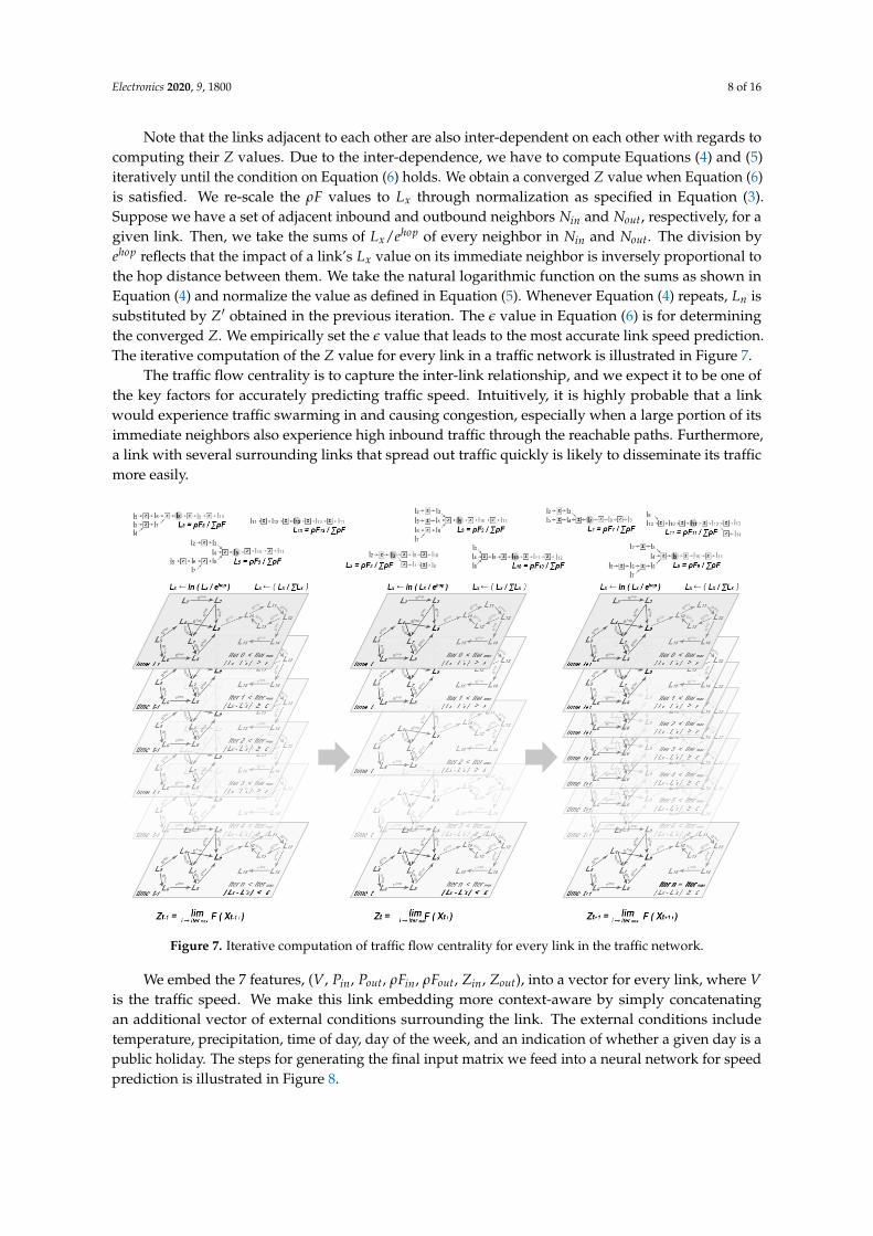
Note that the links adjacent to each other are also inter-dependent on each other with regards tocomputing their Z values. Due to the inter-dependence, we have to compute Equations (4) and (5)iteratively until the condition on Equation (6) holds. We obtain a converged Z value when Equation (6)is satisfied. We re-scale the ρF values to Lx through normalization as specified in Equation (3).Suppose we have a set of adjacent inbound and outbound neighbors Nin and Nout, respectively, for agiven link. Then, we take the sums of Lx/ehop of every neighbor in Nin and Nout. The division byehop reflects that the impact of a link’s Lx value on its immediate neighbor is inversely proportional tothe hop distance between them. We take the natural logarithmic function on the sums as shown inEquation (4) and normalize the value as defined in Equation (5). Whenever Equation (4) repeats, Ln issubstituted by Z′ obtained in the previous iteration. The ε value in Equation (6) is for determiningthe converged Z. We empirically set the ε value that leads to the most accurate link speed prediction.The iterative computation of the Z value for every link in a traffic network is illustrated in Figure 7.

The traffic flow centrality is to capture the inter-link relationship, and we expect it to be one ofthe key factors for accurately predicting traffic speed. Intuitively, it is highly probable that a linkwould experience traffic swarming in and causing congestion, especially when a large portion of itsimmediate neighbors also experience high inbound traffic through the reachable paths. Furthermore,a link with several surrounding links that spread out traffic quickly is likely to disseminate its trafficmore easily.

Figure 7. Iterative computation of traffic flow centrality for every link in the traffic network.

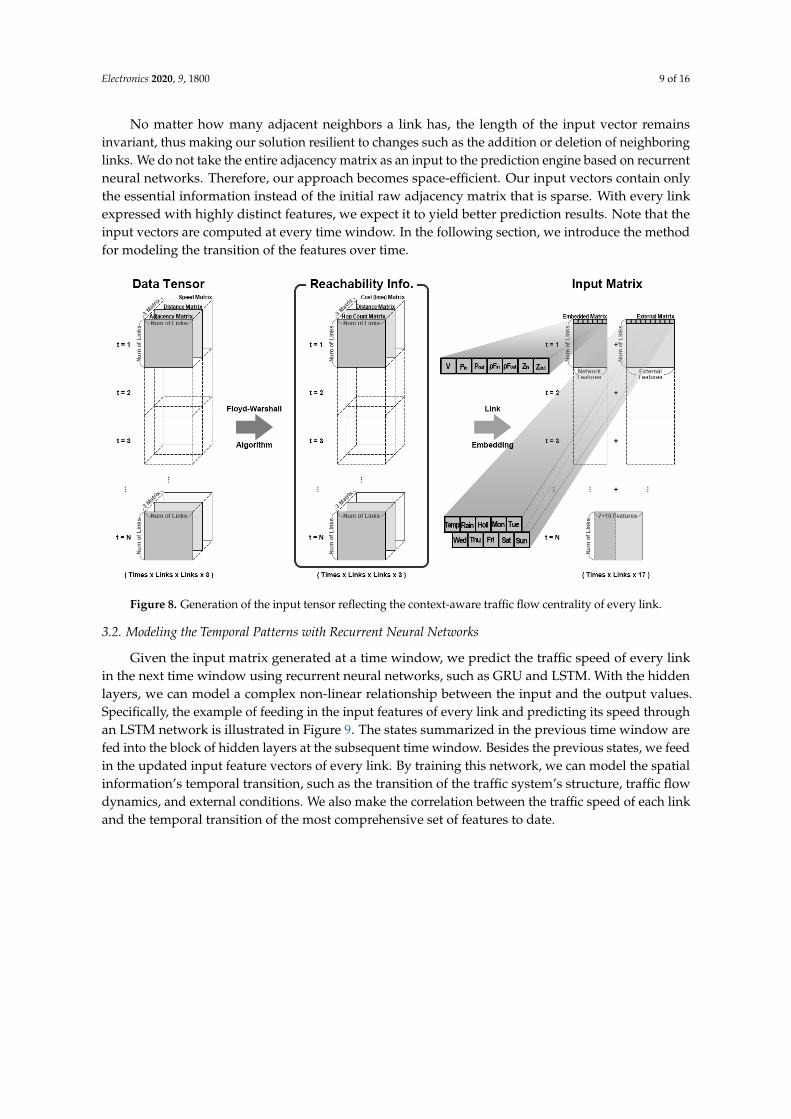
We embed the 7 features, (V, Pin, Pout, ρFin, ρFout, Zin, Zout), into a vector for every link, where Vis the traffic speed. We make this link embedding more context-aware by simply concatenatingan additional vector of external conditions surrounding the link. The external conditions includetemperature, precipitation, time of day, day of the week, and an indication of whether a given day is apublic holiday. The steps for generating the final input matrix we feed into a neural network for speedprediction is illustrated in Figure 8.

Electronics 2020, 9, 1800 9 of 16

No matter how many adjacent neighbors a link has, the length of the input vector remainsinvariant, thus making our solution resilient to changes such as the addition or deletion of neighboringlinks. We do not take the entire adjacency matrix as an input to the prediction engine based on recurrentneural networks. Therefore, our approach becomes space-efficient. Our input vectors contain onlythe essential information instead of the initial raw adjacency matrix that is sparse. With every linkexpressed with highly distinct features, we expect it to yield better prediction results. Note that theinput vectors are computed at every time window. In the following section, we introduce the methodfor modeling the transition of the features over time.

Figure 8. Generation of the input tensor reflecting the context-aware traffic flow centrality of every link.

3.2. Modeling the Temporal Patterns with Recurrent Neural Networks

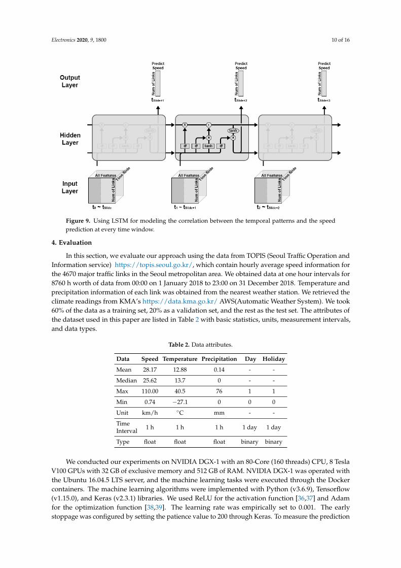
Given the input matrix generated at a time window, we predict the traffic speed of every linkin the next time window using recurrent neural networks, such as GRU and LSTM. With the hiddenlayers, we can model a complex non-linear relationship between the input and the output values.Specifically, the example of feeding in the input features of every link and predicting its speed throughan LSTM network is illustrated in Figure 9. The states summarized in the previous time window arefed into the block of hidden layers at the subsequent time window. Besides the previous states, we feedin the updated input feature vectors of every link. By training this network, we can model the spatialinformation’s temporal transition, such as the transition of the traffic system’s structure, traffic flowdynamics, and external conditions. We also make the correlation between the traffic speed of each linkand the temporal transition of the most comprehensive set of features to date.

Electronics 2020, 9, 1800 10 of 16

Figure 9. Using LSTM for modeling the correlation between the temporal patterns and the speedprediction at every time window.

4. Evaluation

In this section, we evaluate our approach using the data from TOPIS (Seoul Traffic Operation andInformation service) https://topis.seoul.go.kr/, which contain hourly average speed information forthe 4670 major traffic links in the Seoul metropolitan area. We obtained data at one hour intervals for8760 h worth of data from 00:00 on 1 January 2018 to 23:00 on 31 December 2018. Temperature andprecipitation information of each link was obtained from the nearest weather station. We retrieved theclimate readings from KMA’s https://data.kma.go.kr/ AWS(Automatic Weather System). We took60% of the data as a training set, 20% as a validation set, and the rest as the test set. The attributes ofthe dataset used in this paper are listed in Table 2 with basic statistics, units, measurement intervals,and data types.

Table 2. Data attributes.

Data Speed Temperature Precipitation Day Holiday

Mean 28.17 12.88 0.14 - -

Median 25.62 13.7 0 - -

Max 110.00 40.5 76 1 1

Min 0.74 −27.1 0 0 0

Unit km/h ◦C mm - -

TimeInterval 1 h 1 h 1 h 1 day 1 day

Type float float float binary binary

We conducted our experiments on NVIDIA DGX-1 with an 80-Core (160 threads) CPU, 8 TeslaV100 GPUs with 32 GB of exclusive memory and 512 GB of RAM. NVIDIA DGX-1 was operated withthe Ubuntu 16.04.5 LTS server, and the machine learning tasks were executed through the Dockercontainers. The machine learning algorithms were implemented with Python (v3.6.9), Tensorflow(v1.15.0), and Keras (v2.3.1) libraries. We used ReLU for the activation function [36,37] and Adamfor the optimization function [38,39]. The learning rate was empirically set to 0.001. The earlystoppage was configured by setting the patience value to 200 through Keras. To measure the prediction

Electronics 2020, 9, 1800 11 of 16

performance, we employed the metrics as follows: (1) MAE (Mean Absolute Error) (Equations (7));(2) RMSE (Root Mean Squared Error) (Equation (8)); and (3) MAPE (Mean Absolute Percentage Error)(Equation (9)). yt and yt are the predicted speed and the actual speed, respectively. n is the numberof test cases. The ε value for checking the convergence of the Z value, as defined in Equation (6),was empirically set as shown in Table 3. With ε = 0.005, we were able to achieve the lowest MAPE.

MAE =1n

n

∑t=1|yt − yt| (7)

RMSE =

√1n

n

∑t=1

(yt − yt)2 (8)

MAPE =1n

n

∑t=1

∣∣∣∣yt − yt

yt

∣∣∣∣ ∗ 100 (%) (9)

Table 3. Prediction performance according to the convergence condition (ε) setting.

Epsilon MAE RMSE MAPE

0.1 2.60 4.40 10.84

0.05 2.69 4.48 11.16

0.01 2.63 4.41 11.07

0.005 2.50 4.28 10.39

0.001 2.69 4.43 11.15

0.0005 2.59 4.36 10.79

0.0001 2.54 4.32 10.51

4.1. Measurement of Prediction Performance

We measured the prediction performance between various approaches denoted as DNN,TFC-DNN, GRU, TFC-GRU, LSTM, and TFC-LSTM. The prefix TFC- stands for Traffic Flow Centrality,and it represents the following seven novel features that we introduced in Section 3, i.e., V, Pin, Pout,ρFin, ρFout, Zin, and Zout. We evaluated the effectiveness of the information about external conditionssuch as climate and date information separately. DNN, GRU, and LSTM are the artificial neuralnetwork architectures we employed for machine learning. Table 4 contains the prediction performanceof each approach. For each model, we picked the empirically best hyper-parameter settings, such asthe number of hidden layers, perceptrons per layer, and the number of time windows for the recurrentneural networks. For double hidden layers, we had 64 and eight perceptrons for the first and the secondlayer, respectively. For a single hidden layer, we used 512 perceptrons. We cited the representativeexisting works that fall under the prediction model categories that do not use our techniques. We didnot compare the methods that could not deal with the traffic networks that scale to thousands oflinks. MSE values during the training and validation stage are plotted on the graphs in Figure 10.MSEs converged at epoch = 400.

The consideration of every link’s external conditions was effective only when used by LSTM andTFC-LSTM. On the other hand, we observed that using the features related to traffic flow centralityconsistently led to improvement over the baseline approaches. However, when both the externalconditions and the features related to traffic flow centrality were used with LSTM, i.e., TFC-LSTM,we achieved the lowest MAPE of 10.39.

Electronics 2020, 9, 1800 12 of 16

Table 4. Comparison of prediction performance.

Prediction Models Usage of Surrounding Hidden Layer Structure # of Time MAE RMSE MAPECondition Information (# of Perceptrons per Layer) Windows

DNN [12,22] No Double layers (64-8) - 4.05 6.25 15.58Yes Double layers (64-8) - 4.36 6.42 17.36

TFC-DNN No Double layers (64-8) - 3.84 5.98 15.27Yes Double layers (64-8) - 3.96 6.01 17.02

GRU [14] No Single layer (512) 18 3.70 5.51 14.42Yes Single Layer (512) 18 7.52 10.20 31.12

TFC-GRU No Single layer (512) 18 2.85 4.60 11.42Yes Single Layer (512) 18 6.20 8.12 22.57

LSTM [13] No Single layer (512) 18 2.88 4.91 11.89Yes Single Layer (512) 18 2.64 4.48 10.87

TFC-LSTM No Single layer (512) 18 2.63 4.47 11.38Yes Single layer (512) 18 2.50 4.28 10.39

The DNN-based approaches without the information about the external conditions performedpoorly compared to the recurrent neural network models because it does not model the temporaltransitions of the link features.

Figure 10. MSEs during training and validation.

4.2. The Effect of Reachable Path Length Cutoff

We noticed that a link in the Seoul traffic system could be reached from any other links withinan hour regardless of the distance, even during rush hours with heavy traffic, according to theFloyd–Warshall algorithm we used for retrieving the lowest cost inbound and outbound paths betweenany OD pairs. It turns out that the Floyd–Warshall algorithm retrieved several unrealistic reachablepaths between any OD pairs by ignoring specific restrictions on some of the traffic links. For example,the algorithm generated some routes that included wild U-turns that are not allowed on some roads.As a result, path lengths measured as the number of hops tended to be excessively long. Thus, we wereunnecessarily taking into account the state of the links for which it is practically impossible to influencethe state of the remote links.

One possible solution to this problem is to have a shorter time window than an hour. However,TOPIS only makes the hourly data available to the public. Therefore, we revised the algorithm tolimit the path length instead. When overall traffic flows at the lowest average speed, we limited thereachable inbound and outbound path lengths to 15 hops. On the other hand, for the period whenoverall traffic flows at the highest average speed, we relaxed the length limit to 45 hops. Furthermore,the link’s low speed may be attributed to the congestion on the neighboring links in the vicinity. Thus,reachability from other links to the low-speed link is also limited. Therefore, it is sufficient to consideronly the links in proximity. Compared to the period of lowest average traffic speed (“Lowest Speed

Electronics 2020, 9, 1800 13 of 16

Period” in Table 5), the reachability of the traffic from one link to the others is higher during thehighest average traffic speed period. Thus, for such a period (“Highest Speed Period” in Table 5),we considered the states of the other links within a wider range. Our simple revision of the algorithmis empirically proven to be effective, as shown in Table 5. It shows the prediction performance fordifferent path length cutoff settings. We observed that our approach performed most effectively withan MAPE of 10.39 when the range of neighboring links to consider was proportional to the traffic’saverage speed.

Table 5. The effect of reachability path length limit on speed prediction.

Lowest Speed Period Highest Speed Period MAE RMSE MAPE

15 hops 15 hops 2.61 4.38 10.83

30 hops 30 hops 2.51 4.30 10.48

45 hops 45 hops 2.61 4.40 10.96

15 hops 45 hops 2.50 4.28 10.39

45 hops 15 hops 2.63 4.44 10.98

4.3. The Discussion on Scalability

One of the merits of our approach is the capability to predict the traffic speeds even for a verylarge-scale traffic network such as the road system of Seoul. The larger the traffic network is, the higherthe opportunity is to predict speed accurately. This is because we can consider more conditions aroundthe links that are often overlooked by the existing works. The works that only consider the conditionsof adjacent neighbors [18] exhibited a decline in prediction accuracy compared to what was originallyreported and performed worse than our approach. This is because their approaches were unabletocapture the farther away links’ highly probable influence.

Naively feeding in the raw adjacency matrix was the most space inefficient approach [40,41].We could not even compare the prediction performance with such approaches, as they quicklyencountered out-of-memory errors when dealing with Seoul’s large-scale road system. Our approachis agnostic of the scale of the network and even the structure change. Regardless of the scale and anychanges, we ran the aggregation functions to compute the fixed-length input feature vector concerningthe traffic flow centrality. Therefore, we did not need to restructure the neural network architectureupon changes to the traffic system (i.e., addition/deletion of links, change of adjacent links).

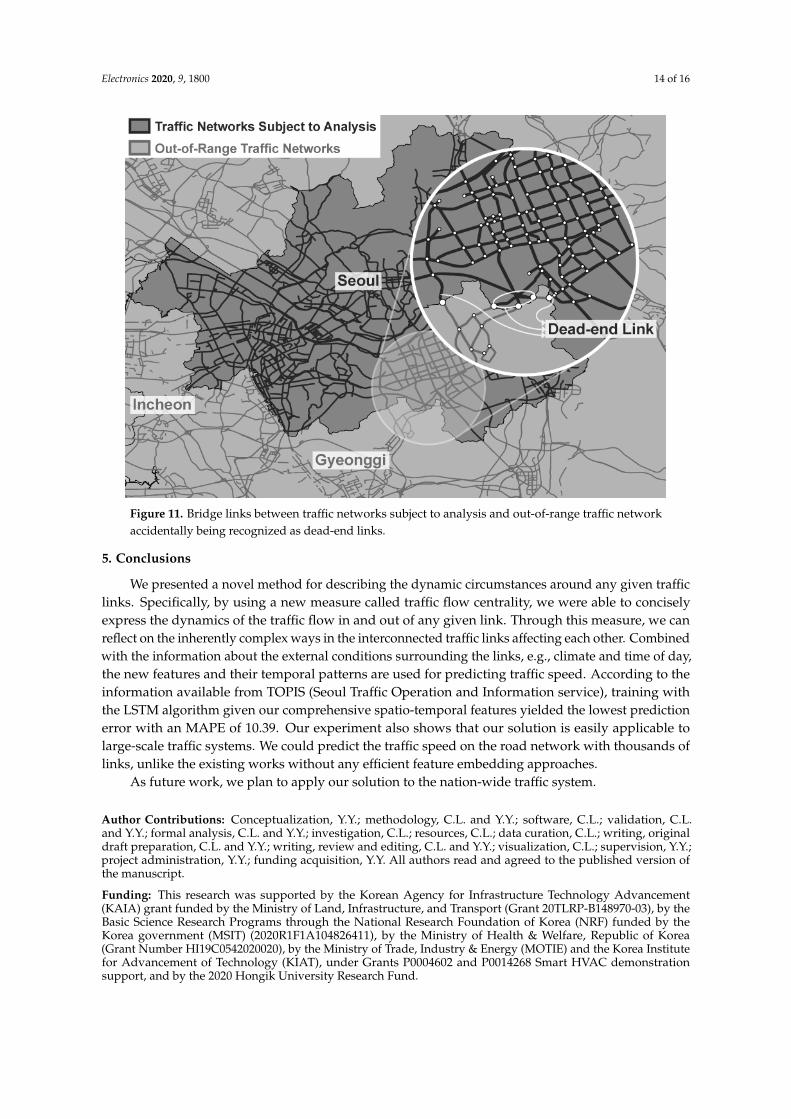
However, we dealt with a fragment of the entire national traffic system in South Korea. The trafficnetworks in Seoul are connected to the systems in other districts such as Gyeonggi Province andIncheon metropolitan area. Due to the fragmented view, we accidentally identified the links that bridgebetween different traffic networks as dead-ends, as shown in Figure 11. We could not accurately reflectthe traffic flow centrality for these dead-end links. The Zout value was zero for these dead-end linksbecause there is no way out. The Zin value is not credible as the inbound traffic from other regions wasnot accounted for. The inaccurate Z values on the dead-end may negatively impact the neighboringlinks’ Z values.

For this issue, we applied the average Z value of the whole system as the Z value of the dead-endlinks, which still cannot be viewed as an ideal solution. This motivated us to venture into applyingour approach to predicting speed prediction for all the links in the entire national traffic system.By expanding the view of the traffic network, we expect the accuracy to improve further. This isplanned to be done soon after we are given integrated traffic information from all Korean regions.

Electronics 2020, 9, 1800 14 of 16

Figure 11. Bridge links between traffic networks subject to analysis and out-of-range traffic networkaccidentally being recognized as dead-end links.

5. Conclusions

We presented a novel method for describing the dynamic circumstances around any given trafficlinks. Specifically, by using a new measure called traffic flow centrality, we were able to conciselyexpress the dynamics of the traffic flow in and out of any given link. Through this measure, we canreflect on the inherently complex ways in the interconnected traffic links affecting each other. Combinedwith the information about the external conditions surrounding the links, e.g., climate and time of day,the new features and their temporal patterns are used for predicting traffic speed. According to theinformation available from TOPIS (Seoul Traffic Operation and Information service), training withthe LSTM algorithm given our comprehensive spatio-temporal features yielded the lowest predictionerror with an MAPE of 10.39. Our experiment also shows that our solution is easily applicable tolarge-scale traffic systems. We could predict the traffic speed on the road network with thousands oflinks, unlike the existing works without any efficient feature embedding approaches.

As future work, we plan to apply our solution to the nation-wide traffic system.

Author Contributions: Conceptualization, Y.Y.; methodology, C.L. and Y.Y.; software, C.L.; validation, C.L.and Y.Y.; formal analysis, C.L. and Y.Y.; investigation, C.L.; resources, C.L.; data curation, C.L.; writing, originaldraft preparation, C.L. and Y.Y.; writing, review and editing, C.L. and Y.Y.; visualization, C.L.; supervision, Y.Y.;project administration, Y.Y.; funding acquisition, Y.Y. All authors read and agreed to the published version ofthe manuscript.

Funding: This research was supported by the Korean Agency for Infrastructure Technology Advancement(KAIA) grant funded by the Ministry of Land, Infrastructure, and Transport (Grant 20TLRP-B148970-03), by theBasic Science Research Programs through the National Research Foundation of Korea (NRF) funded by theKorea government (MSIT) (2020R1F1A104826411), by the Ministry of Health & Welfare, Republic of Korea(Grant Number HI19C0542020020), by the Ministry of Trade, Industry & Energy (MOTIE) and the Korea Institutefor Advancement of Technology (KIAT), under Grants P0004602 and P0014268 Smart HVAC demonstrationsupport, and by the 2020 Hongik University Research Fund.

Electronics 2020, 9, 1800 15 of 16

Conflicts of Interest: The authors declare no conflict of interest. The funders had no role in the design of thestudy; in the collection, analyses, or interpretation of data; in the writing of the manuscript; nor in the decision topublish the results.

Abbreviations

The following abbreviations are used in this manuscript:

OD Origin and DestinationTFC Traffic Flow Centrality (Z value)

References

1. Williams, B.M.; Hoel, L.A. Modeling and Forecasting Vehicular Traffic Flow as a Seasonal ARIMA Process:Theoretical Basis and Empirical Results. J. Transp. Eng. 2003, 129, 664–672.

2. Kumar, S.V.; Vanajakshi, L. Short-Term Traffic Flow Prediction using Seasonal ARIMA Model with LimitedInput Data. Eur. Transp. Res. Rev. 2015, 7, 21.

3. Chen, C.; Hu, J.; Meng, Q.; Zhang, Y. Short-Time Traffic Flow Prediction with ARIMA-GARCH Model.In Proceedings of the 2011 IEEE Intelligent Vehicles Symposium (IV), Baden-Baden, Germany, 5–9 June 2011;pp. 607–612.

4. Jeong, Y.S.; Byon, Y.J.; Castro-Neto, M.M.; Easa, S.M. Supervised Weighting-Online Learning Algorithm forShort-Term Traffic Flow Prediction. IEEE Trans. Intell. Transp. Syst. 2013, 14, 1700–1707.

5. Wu, C.H.; Ho, J.M.; Lee, D.T. Travel-Time Prediction with Support Vector Regression. IEEE Trans. Intell.Transp. Syst. 2004, 5, 276–281.

6. Cai, P.; Wang, Y.; Lu, G.; Chen, P.; Ding, C.; Sun, J. A Spatiotemporal Correlative K-Nearest Neighbor Modelfor Short-Term Traffic Multistep Forecasting. Transp. Res. Part C Emerg. Technol. 2016, 62, 21–34.

7. Kim, T.; Kim, H.; Lovell, D.J. Traffic Flow Forecasting: Overcoming Memoryless Property in NearestNeighbor Non-Parametric Regression. In Proceedings of the 2005 IEEE Intelligent Transportation Systems,2005, Vienna, Austria, 16 September 2005; pp. 965–969.

8. Yin, H.; Wong, S.; Xu, J.; Wong, C. Urban Traffic Flow Prediction using a Fuzzy-Neural Approach. Transp. Res.Part C Emerg. Technol. 2002, 10, 85–98.

9. Quek, C.; Pasquier, M.; Lim, B.B.S. POP-TRAFFIC: A Novel Fuzzy Neural Approach to Road Traffic Analysisand Prediction. IEEE Trans. Intell. Transp. Syst. 2006, 7, 133–146.

10. Guo, S.; Lin, Y.; Li, S.; Chen, Z.; Wan, H. Deep Spatial-Temporal 3D Convolutional Neural Networks forTraffic Data Forecasting. IEEE Trans. Intell. Transp. Syst. 2019, 20, 3913–3926.

11. Lv, Y.; Duan, Y.; Kang, W.; Li, Z.; Wang, F.Y. Traffic Flow Prediction with Big Data: A Deep LearningApproach. IEEE Trans. Intell. Transp. Syst. 2014, 16, 865–873.

12. Koesdwiady, A.; Soua, R.; Karray, F. Improving Traffic Flow Prediction with Weather Information inConnected Cars: A Deep Learning Approach. IEEE Trans. Veh. Technol. 2016, 65, 9508–9517.

13. Tian, Y.; Pan, L. Predicting Short-Term Traffic Flow by Long Short-Term Memory Recurrent NeuralNetwork. In Proceedings of the 2015 IEEE International Conference on Smart City/SocialCom/SustainCom(SmartCity), Chengdu, China, 19–21 December 2015; pp. 153–158.

14. Fu, R.; Zhang, Z.; Li, L. Using LSTM and GRU Neural Network Methods for Traffic Flow Prediction.In Proceedings of the 2016 31st Youth Academic Annual Conference of Chinese Association of Automation(YAC), Wuhan, China, 11–13 November 2016; pp. 324–328.

15. Huang, W.; Song, G.; Hong, H.; Xie, K. Deep Architecture for Traffic Flow Prediction: Deep Belief Networkswith Multitask Learning. IEEE Trans. Intell. Transp. Syst. 2014, 15, 2191–2201.

16. Du, B.; Peng, H.; Wang, S.; Bhuiyan, M.Z.A.; Wang, L.; Gong, Q.; Liu, L.; Li, J. Deep Irregular ConvolutionalResidual LSTM for Urban Traffic Passenger Flows Prediction. IEEE Trans. Intell. Transp. Syst. 2019, 21,972–985.

17. Gu, Y.; Lu, W.; Xu, X.; Qin, L.; Shao, Z.; Zhang, H. An Improved Bayesian Combination Model for Short-TermTraffic Prediction with Deep Learning. IEEE Trans. Intell. Transp. Syst. 2019, 21, 1332–1342.

18. Cui, Z.; Henrickson, K.; Ke, R.; Wang, Y. Traffic Graph Convolutional Recurrent Neural Network: A DeepLearning Framework for Network-Scale Traffic Learning and Forecasting. IEEE Trans. Intell. Transp. Syst.2019. doi:10.1109/TITS.2019.2950416.

Electronics 2020, 9, 1800 16 of 16

19. Hamilton, W.L.; Ying, R.; Leskovec, J. Representation Learning on Graphs: Methods and Applications. arXiv2017, arXiv:1709.05584.

20. Floyd, R.W. Algorithm 97: Shortest Path. Commun. ACM 1962, 5, 345.21. Zhang, J.; Zheng, Y.; Qi, D.; Li, R.; Yi, X. DNN-based Prediction Model for Spatio-temporal Data.

In Proceedings of the 24th ACM SIGSPATIAL International Conference on Advances in GeographicInformation Systems, Burlingame, CA, USA, 31 October–3 November 2016; pp. 1–4.

22. Kim, D.H.; Hwang, K.Y.; Yoon, Y. Prediction of Traffic Congestion in Seoul by Deep Neural Network. J. KoreaInst. Intell. Transp. Syst. 2019, 18, 44–57.

23. Zheng, Z.; Yang, Y.; Liu, J.; Dai, H.N.; Zhang, Y. Deep and Embedded Learning Approach for Traffic FlowPrediction in Urban Informatics. IEEE Trans. Intell. Transp. Syst. 2019, 20, 3927–3939.

24. Sun, S.; Wu, H.; Xiang, L. City-wide traffic flow forecasting using a deep convolutional neural network.Sensors 2020, 20, 421.

25. Hochreiter, S.; Schmidhuber, J. Long Short-Term Memory. Neural Comput. 1997, 9, 1735–1780.26. Krizhevsky, A.; Sutskever, I.; Hinton, G.E. Imagenet Classification with Deep Convolutional Neural

Networks. In Proceedings of the Advances in Neural Information Processing Systems, Lake Tahoe, NV,USA, 3–6 December 2012; pp. 1097–1105.

27. Karpathy, A.; Toderici, G.; Shetty, S.; Leung, T.; Sukthankar, R.; Li, F.-F. Large-Scale Video Classification withConvolutional Neural Networks. In Proceedings of the IEEE conference on Computer Vision and PatternRecognition, Columbus, OH, USA, 23–28 June 2014; pp. 1725–1732.

28. Ji, S.; Xu, W.; Yang, M.; Yu, K. 3D Convolutional Neural Networks for Human Action Recognition. IEEE Trans.Pattern Anal. Mach. Intell. 2012, 35, 221–231.

29. Chung, J.; Gulcehre, C.; Cho, K.; Bengio, Y. Empirical Evaluation of Gated Recurrent Neural Networks onSequence Modeling. arXiv 2014, arXiv:1412.3555.

30. Jia, Y.; Wu, J.; Xu, M. Traffic Flow Prediction with Rainfall Impact using a Deep Learning Method.J. Adv. Transp. 2017, 2017.

31. Yu, B.; Lee, Y.; Sohn, K. Forecasting Road Traffic Speeds by Considering Area-Wide Spatio-temporalDependencies based on a Graph Convolutional Neural Network (GCN). Transp. Res. Part C Emerg. Technol.2020, 114, 189–204.

32. Ge, L.; Li, S.; Wang, Y.; Chang, F.; Wu, K. Global Spatial-Temporal Graph Convolutional Network for UrbanTraffic Speed Prediction. Appl. Sci. 2020, 10, 1509.

33. Lu, H.; Huang, D.; Song, Y.; Jiang, D.; Zhou, T.; Qin, J. St-trafficnet: A spatial-temporal deep learningnetwork for traffic forecasting. Electronics 2020, 9, 1474.

34. Scarselli, F.; Gori, M.; Tsoi, A.C.; Hagenbuchner, M.; Monfardini, G. The Graph Neural Network Model.IEEE Trans. Neural Netw. 2008, 20, 61–80.

35. Kipf, T.N.; Welling, M. Semi-Supervised Classification with Graph Convolutional Networks. arXiv 2016,arXiv:1609.02907.

36. Nair, V.; Hinton, G.E. Rectified Linear Units Improve Restricted Boltzmann Machines; In Proceedings of the27th International Conference on Machine Learning (ICML 2010), Haifa, Israel, 21–24 June 2010.

37. Glorot, X.; Bordes, A.; Bengio, Y. Deep Sparse Rectifier Neural Networks. In Proceedings of the FourteenthInternational Conference on Artificial Intelligence and Statistics, Fort Lauderdale, FL, USA, 11–13 April 2011;pp. 315–323.

38. Kingma, D.P.; Ba, J. Adam: A method for Stochastic Optimization. arXiv 2014, arXiv:1412.6980.39. Ruder, S. An Overview of Gradient Descent Optimization Algorithms. arXiv 2016, arXiv:1609.04747.40. Yu, B.; Yin, H.; Zhu, Z. Spatio-temporal Graph Convolutional Networks: A Deep Learning Framework for

Traffic Forecasting. arXiv 2017, arXiv:1709.04875.41. Zhao, L.; Song, Y.; Zhang, C.; Liu, Y.; Wang, P.; Lin, T.; Deng, M.; Li, H. T-GCN: A Temporal Graph

Convolutional Network for Traffic Prediction. IEEE Trans. Intell. Transp. Syst. 2019, 21, 3848–3858.

Publisher’s Note: MDPI stays neutral with regard to jurisdictional claims in published maps and institutionalaffiliations.

Electronics 2020, 9, 1800 17 of 16

© 2020 by the authors. Licensee MDPI, Basel, Switzerland. This article is an open accessarticle distributed under the terms and conditions of the Creative Commons Attribution(CC BY) license (http://creativecommons.org/licenses/by/4.0/).