Journal of Computational and Applied Mathematics ( ) –

Contents lists available at ScienceDirect

Journal of Computational and AppliedMathematics

journal homepage: www.elsevier.com/locate/cam

Existence and stability of stationary waves of a populationmodel with strong Allee effectMajid Bani-Yaghoub a,∗, Guangming Yao b, Hristo Voulov a

a Department of Mathematics and Statistics, University of Missouri-Kansas City, Kansas City, MO 64110-2499, USAb Department of Mathematics, Clarkson University, Potsdam, NY, 13699-5815, USA

a r t i c l e i n f o

Article history:Received 31 July 2015Received in revised form 23 November2015

MSC:37N2535R10

Keywords:Allee effectDelayReaction–diffusionNonlocalityStationary wave

a b s t r a c t

We investigate the existence and stability of stationary waves of a nonlocal reac-tion–diffusion population model with delay, nonlocality and strong Allee effect. By re-ducing the model, the conditions for existence of stationary wavefront, wave pulse andinverted wave pulse are established. Then we show that the stationary waves of the re-duced model are also the stationary waves of the general model. The global stability of thestationary waves is illustrated by numerically solving the general model for different setsof parameter values.

© 2015 Elsevier B.V. All rights reserved.

1. Introduction

The wave solutions of Reaction–Diffusion (RD) models have been center of attention for decades [1–4]. In addition tovast applications of traveling waves in population biology [5,3,6], various forms of waves have been observed in chemicalreactions [1,7,8], nonlinear optics [9], water waves [10–12], gas dynamics [13] and solid mechanics [14–17]. In order todefine the wave solutions of RD models, consider the following scalar RD equation

du(x, t)dt

= D∂2u(x, t)

∂x2+ f (u(x, t)), (1)

where u(x, t) ∈ R is for instance, the population density of a single species at time t and location x ∈ R, f (u) is theproliferation rate, and D is the diffusion rate of the single species. A traveling wave solution u(x, t) of Eq. (1) is a solution ofthe form

u(x, t) = U(x + ct) = U(z), z = x + ct, with x ∈ R and t > 0, (2)

where the constant c is the speed of propagation and the dependent variable z is the wave variable. Then U(z) is a travelingwavemoving at constant speed c without changing its shape or amplitude. To be physically realistic, U(z)must be bounded

∗ Corresponding author.E-mail address: baniyaghoubm@umkc.edu (M. Bani-Yaghoub).

http://dx.doi.org/10.1016/j.cam.2015.11.0210377-0427/© 2015 Elsevier B.V. All rights reserved.

2 M. Bani-Yaghoub et al. / Journal of Computational and Applied Mathematics ( ) –

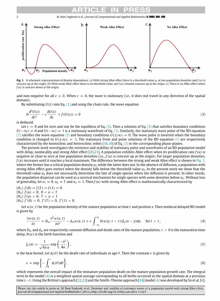
Fig. 1. A schematic representation of density dependence. (a) With strong Allee effect there is a threshold value u2 at low population densities and f (u) isconcave up at the origin. (b) With weak Allee effect there is no threshold value, yet f (u) remains concave up at the origin. (c) There is no Allee effect whenf (u) is concave down at the origin.

and non-negative for all z ∈ R. When c = 0, the wave is stationary (i.e., it does not travel in any direction of the spatialdomain).

By substituting U(z) into Eq. (1) and using the chain rule, the wave equation

Dd2U(z)dz2

− cdU(z)dz

+ f (U(z)) = 0 (3)

is deduced.Let c = 0 and let zero and one be the equilibria of Eq. (3). Then a solution of Eq. (3) that satisfies boundary conditions

U(−∞) = 0 and U(−∞) = 1 is a stationary wavefront of Eq. (1). Similarly, the stationary wave pulse of the RD equation(1) satisfies the wave equation (3) and boundary conditions U(±∞) = 0. The wave pulse is inverted when the boundarycondition is changed to U(±∞) = 1. The stationary front and pulse solutions of the RD equation (1) are respectivelycharacterized by the homoclinic and heteroclinic orbits [18,19] of Eq. (3) in the corresponding phase-planes.

The present work investigates the existence and stability of stationary pulse and wavefronts of an RD population modelwith delay, nonlocality and strong Allee effect [20,21]. A population exhibits Allee effect when its proliferation rate f (u) isnegative or close to zero at low population densities (i.e., f (u) is concave up at the origin). For larger population densities,f (u) increases until it reaches a local maximum. The difference between the strong and weak Allee effect is shown in Fig. 1,where the former has a critical population density u2 while the latter does not. In the absence of diffusion, a population withstrong Allee effect goes extinct when the density falls below the threshold value u2. In the present work we show that thethreshold value u2 does not necessarily determine the fate of single species when the diffusion is present. In other words,the population dispersal can be used as a survival mechanism for single species with some densities below u2. Without lossof generality, let u1 = 0, u2 = T and u3 = 1. Then f (u) with strong Allee effect is mathematically characterized by

(H1) f (0) = f (T ) = f (1) = 0(H2) f (u) < 0, 0 < u < T(H3) f (u) > 0, T < u < 1(H4) f ′(0) < 0, f ′(T ) > 0, f ′(1) < 0.

Let w(x, t) be the population density of the mature population at time t and position x. Then nonlocal delayed RDmodelis given by

∂w(x, t)∂t

= Dm∂2w(x, t)

∂x2− dmw(x, t) + ϵ

∞

−∞

b(w(y, t − τ))fα(x − y)dy, for t > τ, (4)

where Dm and dm are respectively constant diffusion and death rates of themature population, τ > 0 is thematuration timedelay, b(w) is the birth function and

fα(x) =1

√4πα

exp

−x2

4α

, (5)

is the heat kernel. Let dI(θ) be the death rate of individuals at age θ . Then the constant ϵ is given by

ϵ = exp−

τ

0dI(θ)dθ

, (6)

which represents the overall impact of the immature population death on the mature population growth rate. The integralterm in the model (4) is a weighted spatial average corresponding to all births occurred in the spatial domain at a previoustime t−τ . Using the Britton’s approach [22,23] and the Smith–Thieme approach [24]model (4)was developed by So et al. [6].

M. Bani-Yaghoub et al. / Journal of Computational and Applied Mathematics ( ) – 3

The impact of the density dependent birth function b(w) andmaturation time delay τ on single species population dynamicshas been studied in detail [25,26]. Model (4) has also been extended to RD models with respect to two-dimensional spatialdomains [25–27], where the existence of traveling wave solutions has been investigated [26,6].

The diffusion rate of the immature population is given by DI = α/τ . Hence, the immature population is immobile whenα = 0 and the general model (4) is reduced to

∂w(x, t)∂t

= Dm∂2w

∂x2− dmw(x, t) + ϵb(w(x, t − τ)), (7)

which has been extensively studied [28–30].Let w(x, t) = φ(x + ct) = φ(z) be a wave solution of the general model (4). Let Y = y − x and z = x + ct . Define the

linear transformation T (t, x) = x + ct and let w(x, t) = φ(z) be the wave solution. Then substituting φ(z) into (4), usingthe transformation T (t − τ , y) = z − cτ + Y , and replacing Y with y, the wave equation corresponding to (4) is given by

Dmφ′′(z) − cφ′(z) − dmφ(z) + ϵ

∞

−∞

b(φ(z − cτ + y))fα(y)dy = 0. (8)

The minimal speed of spread and the existence of traveling wavefronts of the model (4) have already been investigatedin several studies [5,31,6]. Using specific birth functions, the behavior of wave solutions has been studied in [5,32,26]. Thetraveling wave solution of model (4) can be approximated using a boundary layer method combined with an asymptoticexpansion method [33]. Despite the above-mentioned studies, there has been less effort investigating the existence andstability of the stationary waves of the model (4). The present work aims to fill this gap by establishing the conditionsfor existence of stationary waves (Section 2) and numerically examining the stability of the stationary wave solutions(Section 3). Furthermore, a discussion of the main outcomes and the biological implications of the results is provided inSection 4.

2. Existence of stationary waves

Let c = 0 and U(z) = φ(x). Then wave equation (3) is reduced to the Hamiltonian systemdφ(x)dx

= ϕ(x)

dϕ(x)dx

= −1Df (φ(x)),

(9)

with the Hamiltonian function

H (φ, ϕ) =ϕ2

2+

1D

φ

0f (s)ds. (10)

Define

F(φ) =1D

φ

0f (s)ds. (11)

The following theorem establishes the conditions for existence of homoclinic and heteroclinic orbits of the system (9).

Theorem 1. Let f (φ) be continuous and satisfy conditions (H1)–(H4). Then system (9) admits a

(i) right-homoclinic orbit, when F(1) > 0(ii) left-homoclinic orbit, when F(1) < 0(iii) heteroclinic orbit, when F(1) = 0.

Proof. Part (i)Each level curve of the system (9) is given by H (φ, ϕ) = k, where k is a constant. Noting that H (0, 0) = 0 for a right-

homoclinic orbit, we must have k = 0. Using (10) the level curve passing through the origin must satisfy ϕ2= −2F(φ).

By conditions (H1) and (H2) we get that F(0) = 0 and F(φ) < 0 for φ ∈ (0, T ]. Since F(1) > 0, there must be a pointφ∗

∈ (T , 1) such that F(φ∗) = 0. By the continuity of F(φ) we conclude that there exists a homoclinic orbit connecting theorigin to itself.Part (ii)

A left-homoclinic orbit connects (φ, ϕ) = (1, 0) to itself. Consider the slightly modified Hamiltonian function

H (φ, ϕ) =ϕ2

2−

1D

1

φ

f (s)ds. (12)

4 M. Bani-Yaghoub et al. / Journal of Computational and Applied Mathematics ( ) –

Similar to part (i), for the level curve passing through (1, 0), we must have k = 0 and therefore ϕ2=

2D

1φf (s)ds. By

conditions (H1) and (H4) the last integral has a maximum at φ = T and declines in the interval φ ∈ (T , 1). Noting thatF(1) < 0, there must be a point φ∗

∈ (0, T ) such that ϕ = 0.Part (iii)

A heteroclinic orbit connects the origin to (φ, ϕ) = (1, 0). Since F(1) = 0 we must have 1T f (s)ds = −

T0 f (s)ds. Using

the Hamiltonian function (10) we get that φ∗= 1. �

A non-constant stationary solution w(x, t) = φ(x) of the reduced model (7) must satisfy

Dmφ′′(x) − dmφ(x) + ϵb(φ(x)) = 0. (13)

Then we have the following corollary.

Corollary 1. Let f (φ) = ϵb(φ) − dmφ and satisfy conditions (H1)–(H4). Then the reduced model (7) admits a stationary

(i) wave pulse, when F(1) > 0(ii) inverted wave pulse, when F(1) < 0(iii) wavefront, when F(1) = 0.

Proof. This is a direct implication of Theorem 1. �

We now turn our attention to the specific birth function given by

b(φ) = pφ2e−aφ, (14)

which has been frequently used in different studies [32,31,26,6]. The single species population can exhibit strongAllee effect,when the birth function (14) is employed. The following lemma provides details of the possible equilibria of models (4) and(7) with the birth function (14).

Lemma 1. Let b(φ) = pφ2e−aφ . Let ϵp/dm = era/r for r > 0 and r = 1. Then the reduced and general models (7) and (4) bothadmit constant equilibria φ1 = 0, 0 < φ2 < φ3 and φ3 = r/a.

Proof. A constant equilibriumφi of the reducedmodel (7) is also that of the generalmodel (4) and it satisfies ϵb(φi)−dmφi =

0. When b(φ) = pφ2e−aφ, φ1 = 0 is an equilibrium. Provided that r > 0 and r = 1, there are two positive equilibria

φ2 = −W0(−adm/ϵp)/a and φ3 = −W−1(−adm/ϵp)/a,

where W0(x) and W−1(x) represent the real-valued principal and the lower branches of Lambert W (x) function, for x ∈

(−e−1, 0). Using ϵp/dm = era/r we get that φ3 = r/a and 0 < φ2 < φ3. �

The following corollary establishes the conditions for existence of stationarywaves of the reducedmodel (7), when the birthfunction (14) is employed.

Corollary 2. Let b(φ) = pφ2e−aφ . Let h(r) = −2er/r + r2/2 + r + 2 + 2/r, r = 1 and ϵp/dm = era/r. Then the reducedmodel (7) admits a stationary

(i) wave pulse, when h(r) < 0(ii) inverted wave pulse, when h(r) > 0(iii) wavefront, when h(r) = 0.

Proof. Noting that f (φ) = ϵb(φ) − dmφ from Eq. (14) we havef (φ)dφ = −ϵp

a2φ2

+ 2aφ + 2a3

e−aφ

−dm2

φ2. (15)

Part (i) Using Theorem 1 we only need to show that F(1) > 0 or equivalently φ3

φ2

f (φ)dφ > −

φ2

0f (φ)dφ. (16)

Using Eq. (15) and noting that the equilibria φi, i = 1, 2, 3 satisfy dmφ = ϵpφ2e−aφ we get that the inequality (16) is thesame as

dm

φ23

2+

φ3

a+

2a2

+2

a3φ3

<

2ϵpa3

. (17)

By Lemma 1 φ3 = r/a. Also ϵp/dm = era/r . Hence the last inequality is the same as h(r) < 0. Proofs of parts (ii) and (iii)are similar to the proof of part (i). �

M. Bani-Yaghoub et al. / Journal of Computational and Applied Mathematics ( ) – 5

Remark 1. Note that the root of h(r) is r = 1.451. Hence, under the assumptions of Corollary 2 the reduced model (7)admits a stationary wavefront when r = 1.451. Similarly, the existence of inverted wave pulse and wave pulse are impliedby r < 1.451 and r > 1.451, respectively.

The following theorem indicates that the stationary pulse and front solutions of the reduced model (7) are also those ofthe general model (4). The proof is based on the generalizedmean value theorem and the properties of the heat kernel fα(x).

Remark 2. Let f (x) and g(x) be continuous functions. Let f (x) ≥ 0 for all x ∈ R and a, b > 0. Then by the mean valuetheorem for integrals (e.g., [34, page 409]), there exists a constant k > 0 such that b

−ag(t)f (t)dt = g(k)

b

−af (t)dt. (18)

Theorem 2. Let φ(x) be a stationary front, pulse or inverted pulse of the reduced model (7). Then φ(x) is also a stationary front,pulse or inverted pulse of the general model (4), respectively.

Proof. Let φ(x) be the stationary front of the reduced model (7) that connects the equilibria φ+ and φ− at the two ends.Then φ(x) satisfies

Dmφ′′(x) − dmφ(x) + ϵb(φ(x)) = 0. (19)

We need to show that φ(x) also satisfies the wave equation of the general model (4), which is

Dmφ′′(x) − dmφ(x) + ϵ

∞

−∞

b(φ(y))fα(x − y)dy = 0. (20)

Let z = y − x − v, where v is a constant which is determined later. Noting that fα(x) defined in (5) has the propertyfα(x − y) = fα(y − x), Eq. (20) is rewritten

Dmφ′′(z) − dmφ(z) + ϵ

∞

−∞

b(φ(z + x + v))fα(z + v)dz = 0. (21)

Hence, we need to show that for each x ∈ R,∞

−∞

b(φ(z + x + v))fα(z + v)dz = b(φ(x)). (22)

Let a and b be positive constants. Noting that b(φ(z + x)) and fα(z) are continuous and fα(z) > 0 for all z ∈ R, by Remark 2,for each x ∈ R there exists a constant k ∈ (−a, b) such that b

−ab(φ(z + x + v))fα(z + v)dz = b(φ(k + x + v))

b

−afα(z + v)dz. (23)

The value of k depends on a and b. However, the only extrema of fα(z) is the global maximum at z = 0 and lim fα(z) = 0and lim b(φ(z)) = b(φ±), as z → ±∞.Also the integrals in (23) are convergent and

∞

−∞fα(z + v)dz = 1. Hence by letting a, b → ∞, k converges to a single value

k∗, where v = k∗ implies Eq. (22). The proof for the stationary pulse or inverted pulse is similar. �

3. Stability of stationary waves

Stability of stationary wave solutions was numerically investigated by solving the initial value problem corresponding tothe general model (4) and the wave equation (13). In particular, we employed a finite difference scheme in Matlab 2014a tosolve and compare the PDE solutions of (4) with the stationary wave solutions of (13) for different sets of parameter values.When a stationary wave solution exists, the choice of the initial history function can play a critical role in convergence ofthe PDE solution to the wave solution or to the constant equilibria. By considering the birth function (14), there are threeconstant equilibria φ1 = 0, φ2 = −W0(−adm/ϵp)/a and φ3 = −W−1(−adm/ϵp)/a, provided ϵp/dm > ae. Noting thatφ1 and φ3 are stable and φ2 is unstable, we need to choose a history function w0(x, t) with values below and above φ2.Otherwise the PDE solution converges to φ1 regardless of the delay value τ or it converges to φ3 for small values of τ . Weconsidered the initial history function

w0(x, t) = φ2 − y0 + β/(1 + exp(−δ(x − 210))) for t ∈ [−τ , 0] (24)

6 M. Bani-Yaghoub et al. / Journal of Computational and Applied Mathematics ( ) –

Fig. 2. The solution of the general model (4) may converge to the stationary wavefront. (a) Graph of the proliferation function f (u) = ϵb(u)− dmu, whereb(u) and F(φ) are defined in (14) and (11), respectively. Note that F(1) = 0, i.e., the areas surrounded by f (u) and u-axis are equal. (b) Phase-plane of thesystem (9) representing the heteroclinic orbit. (c and d) Convergence of the solution w(x, t) of the general model (4) to the stationary wavefront φ(x) ofthe wave equation (13). See the supplementary file ‘‘confront.gif’’ for the related animation (see Appendix A). The specific parameter values are given inTable 1.

Table 1Summary of the parameter values used for the numerical simulations illustrated in Figs. 2–4. We used birth function (14)with strong Allee effect for the simulations.

Symbol Description of parameters and variables Specific parameter valuesFig. 2 Fig. 3 Fig. 4

dm Death rate of mature population 0.1 0.1 0.1p Mating ratio 4.27 4.95 3.67ϵ Total death rate of immature population 0.1 0.1 0.1Dm Diffusion rate of mature population 3.0 3.0 3.0DI Diffusion rate of immature population 1.0 1.0 1.0a Overcrowding parameter 1.45 1.60 1.30τ Maturation time delay 1.0 1.0 1.0w2 The equilibrium between 0 and 0.45 0.36 0.58y0 Parameter of the history function 0.1 0.1 0.07β Parameter of the history function 0.2 0.2 0.1δ Parameter of the history function 0.043 0.001 0.008

Notes. The initial history function for Fig. 2 is given by (24). Also the initial history function for Figs. 3 and 4 is given by (25).Similar results were obtained using different sets of parameter values.

and

w0(x, t) = φ2 − y0 + β exp(−δ(x − 200)) for t ∈ [−τ , 0] (25)

to investigate the convergence to the stationarywavefront andwave pulses, respectively. Table 1 is a summary of the specificparameter values including the constants β, δ and y0.

M. Bani-Yaghoub et al. / Journal of Computational and Applied Mathematics ( ) – 7

Fig. 3. The solution of the general model (4) may converge to the stationary wave pulse. (a) Graph of the proliferation function f (u) = ϵb(u)−dmu, whereb(u) is defined in (14). Note that F(1) > 0. i.e., the area above f (u), u ∈ [0, u2] is less than the area under f (u), u ∈ [u2, u3]. (b) Phase-plane of system (9)representing a right-homoclinic orbit. (c and d) Convergence of the solution w(x, t) of model (4) to the stationary wave pulse φ(x) of wave equation (13).See the supplementary file ‘‘conpulse.gif’’ for the related animation (see Appendix A). The expected and actual survival ranges correspond to the absenceand presence of diffusion, respectively. It can be seen that the survival range is increased when the diffusion is present. The specific parameter values aregiven in Table 1.

Fig. 2 shows that the solution of the general model (4) may converge to the stationary wavefront satisfying bothEqs. (8) and (13). Specifically, as shown in panel (a), the existence of the heteroclinic orbit is only possible when F(1) = 0(see Corollary 1 part (iii)). Panel (b) illustrates the phase-plane of the system (9) representing the heteroclinic orbit, which isequivalent to a stationary wavefront. The convergence of the PDE solution to the stationary wavefront is shown in panels (c)and (d). The convergence is animated in ‘‘confront.gif’’ which is available in the supplementary documents (see Appendix A).The specific parameter values are given in Table 1. Further numerical simulations are presented in Figs. 3 and 4, where theconvergence to the stationarywave pulse and invertedwave pulse are shown, respectively. The animation related to the PDEsolution converging towave pulse is available in the supplementary documents (see file ‘‘conpulse.gif’’, Appendix A). Also thefile ‘‘coninvertpulse.gif’’ is the animation for convergence of the PDE solution to the inverted pulse wave. We also exploredthe convergence to the stationary wave solutions for different sets of the parameter values. When the maturation timedelay τ is increased the stability of φ3 is lost for the cases F(1) ≥ 0 (see Theorem 3(iii) of [32]) and therefore convergenceto the stationary wavefront and wave pulse does not occur. Nevertheless, the stability of φ3 is delay independent for thecase F(1) < 0 ([32, Theorem 3(i)]) and the PDE solution may converge to the inverted wave pulse (see Fig. 4) regardless ofτ value.

In addition to convergence to the stationary pulse, panel (d) of Fig. 3 shows that the threshold property of the middleequilibrium w2 = T does not hold valid when the diffusion is present. In particular, the Expected Survival Range (ESR)indicates the regions with the initial population densities above the threshold T and single species with initial densitiesbelow T is expected to go extinct. Whereas the Actual Survival Range (ASR) is wider than the ESR. Hence, the diffusion ofsingle species could act as a survival mechanism for species with initial densities below w2 = T , but nearby ESR. Moreover,panel (d) of Fig. 4 shows that ESR does not cover the entire special domain, but the diffusion may give rise to survivaleverywhere.

8 M. Bani-Yaghoub et al. / Journal of Computational and Applied Mathematics ( ) –

Fig. 4. The solution of the generalmodel (4)may converge to the stationary invertedwave pulse. (a) Graph of the proliferation function f (u) = ϵb(u)−dmu,with F(1) < 0 i.e., the area above f (u), u ∈ [0, u2] is greater than the area under f (u), u ∈ [u2, u3]. (b) Phase-plane of the system (9) representing a left-homoclinic orbit. (c and d) Convergence of the solution w(x, t) of model (4) to the stationary inverted wave pulse φ(x) of the wave equation (13). See thesupplementary file ‘‘coninvertpulse.gif’’ for the related animation (see Appendix A). In the absence of diffusion, the expected survival range corresponds tothe regions with initial population densities above the threshold equilibrium T = u2 . Whereas the actual survival range corresponds to the entire specialdomain. The specific parameter values are given in Table 1.

4. Discussion

There have been widespread and extensive studies on delay diffusive models describing different biological situations.The population models based on Smith–Thieme and Britton’s approaches [22–24] have brought intensive activities todifferent areas of biology such as ecology, epidemiology and population biology. The local and global dynamics of thesemodels are still of great interest and the possible outcomes of these models may bring significant insights in understandingthe complicated nature of population growth and dispersal.

The primary focus of the present work was to investigate the existence and global stability of the stationary waves ofboth reduced and general models (7) and (4). As mentioned in Theorem 2 a stationary wave solution of the reduced model(7) is also a stationary wave solution of the general model (4). The numerical simulations suggest that the solution of thegeneral model (4) may converge to the stationary wave solution satisfying Eqs. (8) and (13). The general model (4) may alsoadmit stationary waves that are not those of the reduced model (7). Such stationary waves were not investigated in thispaper. Formation of the stationary wave pulses and wavefront may reflect population establishment and colonization incertain regions of the wildlife habitats. The biological interpretations of conditions (H1)–(H4) and their subsequent results(i.e., Theorem1 andCorollaries 1 and 2) are briefly discussed as follows. In the absence of population dispersal (i.e., diffusion),a single species population with strong Allee effect is expected to go extinct when the density falls below the threshold T .However, the present work shows that population dispersal may contribute to survival of species with initial densitiesless than T . For instance, Fig. 3(d) shows that a single species with initial densities below T = 0.36 but in the range150 < x < 250 may survive due to existence of a stable stationary wave pulse. Figs. 2(c) and 3(c) show that the actualsurvival regions may not necessarily match with the regions that have initial densities above T = 0.45 and T = 0.36,respectively. This is due to the fact that the shape of and amplitude of the stationary waves are not the same as theinitial density curves defined by Eqs. (24) and (25), respectively. Therefore, the fate of the single species population can

M. Bani-Yaghoub et al. / Journal of Computational and Applied Mathematics ( ) – 9

be determined according to the shape (i.e., front, pulse or inverted pulse) of the globally stable stationary wave rather thana single threshold value T .

In conclusion, the present study was an effort to explore the existence and stability of the stationary waves of singlespecies populations. Formation of the stationary waves in the spatial domain indicates that a constant threshold densitydoes not necessarily determine the survival or extinction of single species with strong Allee effect.

Acknowledgment

This work was partially supported by the University of Missouri Research Board grant (ID: KZ016055).

Appendix A. Supplementary data

Supplementary material related to this article can be found online at http://dx.doi.org/10.1016/j.cam.2015.11.021.

References

[1] M. Bani-Yaghoub, D.E. Amundsen, Dynamics of notch activity in a model of interacting signaling pathways, Bull. Math. Biol. 72 (4) (2010) 780–804.[2] N.F. Britton, Reaction–Diffusion Equations and their Applications to Biology, Academic Press, New York, 1986.[3] P. Grindrod, The Theory and Applications of Reaction–Diffusion Equations–Patterns and Waves, Oxford Univ. Press, New York, 1996.[4] J.H. Wu, Theory and Applications of Partial Functional Differential Equations, in: Applied Math. Sci., vol. 119, Springer-Verlag, New York, 1996.[5] M. Bani-Yaghoub, D.E. Amundsen, Oscillatory traveling waves for a population diffusion model with two age classes and nonlocality induced by

maturation delay, J. Comput. Appl. Math. 34 (1) (2014) 309–324.[6] J.W.-H. So, J. Wu, X. Zou, A reaction–diffusion model for a single species with age-structure. I Traveling wavefronts on unbounded domains, Proc. R.

Soc. Lond. Ser. A Math. Phys. Eng. Sci. 457 (2001) 1841–1853.[7] R. Kapral, K. Showalter (Eds.), Chemical Waves and Patterns, Kluwer, Doordrecht, 1995.[8] A.I. Volpert, V.A. Volpert, V.A. Volpert, TravelingWave Solutions of Parabolic Systems, in: Translations ofMathematicalMonographs, vol. 140, American

Mathematical Society, Providence, RI, 1994.[9] N. Akhmediev, A. Ankiewicz, Solitons: Nonlinear Pulses and Beams, Chapman and Hall, London, 1997.

[10] L. Debnath, Nonlinear Water Waves, Academic Press, Boston, 1994.[11] F. Dias, C. Kharif, Nonlinear gravity and capillary–gravity waves, Annu. Rev. Fluid Mech. 31 (1999) 301–346.[12] R.S. Johnson, A Modern Introduction to the Mathematical Theory of Water Waves, Cambridge Univ. Press, Cambridge, 1997.[13] J. Smoller, Shock Waves and Reaction–Diffusion Equations, Springer, New York, 1994.[14] P.C. Fife, Patterns formation in gradient systems, in: B. Fiedler, G. Iooss, N. Kopell (Eds.), Handbook of Dynamical Systems III: Towards Applications,

Elsevier, Amsterdam, 2000.[15] H.L. Smith, Monotone Dynamical Systems: An Introduction to the Theory of Competitive and Cooperative Systems, American Mathematical Society,

1995, ISBN: 10: 082180393X.[16] H. Smith, H. Thieme, Strongly order preserving semiflows generated by functional differential equations, J. Differ. Equ. 93 (1991) 332–363.[17] H.R. Thieme, Mathematics in Population Biology, Princeton University Press, Princeton, 2003.[18] J. Guckenheimer, P. Holmes, Nonlinear Oscillations, Dynamical Systems, and Bifurcations of Vector Fields, Springer-Verlag, New York, 1983.[19] D.W. Jordan, P. Smith, Nonlinear Ordinary Differential Equations: An Introduction to Dynamical Systems, Oxford University Press, 1999.[20] W.C. Allee, Animal aggregations, Q. Rev. Biol. 2 (1927) 367–398.[21] W.C. Allee, Animal Aggregations: A Study in General Sociology, Chicago Univ. Press, Chicago, 1933.[22] N.F. Britton, Aggregation and the competitive exclusion principle, J. Theoret. Biol. 136 (1) (1989) 57–66.[23] N.F. Britton, Spatial structures and periodic travelling waves in an integro-differential reaction–diffusion populationmodel, SIAM J. Appl. Math. 50 (6)

(1990) 1663–1688.[24] H. Smith, H. Thieme, Strongly order preserving semiflows generated by functional differential equations, J. Differential Equations 93 (1991) 332–363.[25] M. Bani-Yaghoub, G. Yao, Modeling and numerical simulations of single species dispersal in symmetrical domains, Int. J. Appl. Math. 27 (6) (2014)

525–547.[26] D. Liang, J. Wu, F. Zhang, Modelling population growth with delayed nonlocal reaction in 2-dimensions, Math. Biosci. Eng. 2 (1) (2005) 111–132.[27] P. Weng, D. Liang, J. Wu, Asymptotic patterns of a structured population diffusing in a two-dimensional strip, Nonlinear Anal. 69 (2008) 3931–3951.[28] M.C.Memory, Bifurcation and asymptotic behaviour of solutions of a delay-differential equationwith diffusion, SIAM J.Math. Anal. 20 (1989) 533–546.[29] J.W.-H. So, J. Wu, Y. Yang, Numerical Hopf bifurcation analysis on the diffusive Nicholson’s blowflies equation, Appl. Math. Comput. 111 (2000) 53–69.[30] J.W.-H. So, Y. Yang, Dirichlet problem for the diffusive Nicholson’s blowflies equation, J. Differential Equations 150 (1998) 317–348.[31] D. Liang, J. Wu, Travelling waves and numerical approximations in a reaction advection diffusion equation with nonlocal delayed effects, J. Nonlinear

Sci. 13 (2003) 289–310.[32] M. Bani-Yaghoub, G. Yao, M. Fujiwara, D.E. Amundsen, Understanding the interplay between density dependent birth function and maturation time

delay using a reaction–diffusion population model, Ecol. Complex. 21 (2015) 14–26.[33] M. Bani-Yaghoub, Approximate traveling wave solution for a delayed nonlocal reaction–diffusion equation, J. Appl. Math. Comput. (2015)

http://dx.doi.org/10.1007/s12190-015-0958-7.[34] R.W. Hamming, Methods of Mathematics Applied to Calculus, Probability, and Statistics, Dover ed., Dover Publications, 2004.