contents lists available at sciencedirect journal of...

J. of Multi. Fin. Manag. 20 (2010) 35–47

Contents lists available at ScienceDirect

Journal of Multinational FinancialManagement

journal homepage: www.elsevier.com/locate/econbase

Correlation dynamics of global industry portfolios�

Miguel A. Ferreiraa, Paulo M. Gamab,∗

a Universidade Nova de Lisboa, Faculdade de Economia, Portugalb Universidade de Coimbra, FEUC/ISR-Coimbra, Av. Dias da Silva, 165, 3004-512 Coimbra, Portugal

a r t i c l e i n f o

Article history:Received 26 February 2008Accepted 30 November 2009Available online 5 December 2009

JEL classification:G11G15F30

Keywords:CorrelationGlobal industry portfoliosAsymmetries

a b s t r a c t

This paper investigates the time series of realized correla-tions between global industries and the world market over the1979–2008 period. The behavior of industry correlations is char-acterized by long-term swings, with a period of historically lowcorrelations in the late 1990s. The Telecommunications and theFinancials industries show a positive secular trend. Global industrycorrelations move countercyclically. Furthermore, there is evidencethat industry correlations are higher for market downside movesthan for upside moves.

© 2009 Elsevier B.V. All rights reserved.

1. Introduction

Do global industry correlations change over time? Do industry correlations behave differentlydepending on downside or upside movements? These questions are important for several applicationssuch as portfolio selection and risk management. In portfolio selection, if correlations change overtime, the number of industries needed to achieve a given level of diversification also changes overtime. And if all stocks tend to fall together when the market falls, portfolios become less diversifiedjust when that benefit is most needed. In risk management, correlation is a crucial input in estimationof measures of portfolio Value-at-Risk.

Heston and Rouwenhorst (1994) have shown that pure country factors dominate pure global indus-try factors. Since then, several authors find evidence supporting the growing importance of global

� We thank Yakov Amihud, Andrew Ang, Peter Ritchken, and Maria Vassalou for their comments and suggestions.∗ Corresponding author. Tel.: +351 239 790523.

E-mail address: [email protected] (P.M. Gama).

1042-444X/$ – see front matter © 2009 Elsevier B.V. All rights reserved.doi:10.1016/j.mulfin.2009.11.003

http://www.sciencedirect.com/science/journal/1042444X

http://www.elsevier.com/locate/econbase

mailto:[email protected]

dx.doi.org/10.1016/j.mulfin.2009.11.003

36 M.A. Ferreira, P.M. Gama / J. of Multi. Fin. Manag. 20 (2010) 35–47

industry factors over country-specific factors in determining equity returns; see L’Her et al. (2002)and Cavaglia et al. (2004).

Bekaert et al. (2009) dispute the conclusion that industry factors have gained in impor-tance, contending that any decline in industry portfolios correlation during the 1990s has beenreversed. Lower country-return correlations relative to industry-return correlations would supportthe Heston–Rouwenhorst conclusions that country factors dominate industry factors.

We know a considerable amount about cross-country correlation (see, for example, Longin andSolnik, 1995, 2001). So far, however, there is little to no empirical analysis of the correlation of globalindustries. Our goal is thus to contribute to the literature on international investment by character-izing global industry portfolio correlation dynamics in terms of long-term trends and asymmetries.Moreover, global industries presumably diversify away country-specific sources of return variation,and thus allow for a new perspective on the global stock correlations minimizing the dynamics ofcountry factors in explaining the variation of returns.

Our methodology is characterized by several distinct features. First, we use a simple and time-varying measure of correlation—realized correlation (see, for example, Andersen et al., 2001). We usedaily index return data (in each month) to construct a time series of correlation at the monthly fre-quency, which we treat as “observable” and consequently suitable for posterior analysis using standardeconometric models.1

Second, we study the time series behavior and asymmetries in global industry correlations with theworld market portfolio. We use the FTSE/Dow Jones Industry Classification with 42 sectors groupedinto ten industries. The industry grouping allows for insights on easily identified individual industrygroups, based on a correlation measure that by the averaging process minimizes noise.

Finally, we use time-varying estimates of correlation to investigate asymmetries relative to theaggregate market movement (up and down), for the global industry groups.

The literature offers some key results that are related to our work. In the case of cross-countrycorrelations, Longin and Solnik (1995) and Solnik and Roulet (2000) show that correlation is timeunstable, with tendency to increase over time; Solnik et al. (1996) show that correlation is positivelyrelated to the level of country volatility; Longin and Solnik (2001) that correlation is higher in bearmarkets; and Erb et al. (1994) that correlation is related to the coherence between a country’s businesscycles and its market phase.

In the case of global industry portfolios, Ferreira and Gama (2005) find between 1974 and 2001 nonoticeable long-term trend in industry-specific or world portfolio risk (in developed markets). Yet thelate 1990s are characterized by an increase in the ratio between global industry-specific risk and worldrisk; this implies a reduced global industry portfolio correlation during the late 1990s. Moreover, weknow that for local US industry portfolios, correlation with the US market tends to increase for downmarket periods. However, different testing procedures yield different conclusions on the statisticalsignificance of that increase (Ang and Chen, 2002; Hong et al., 2007).

We establish several empirical findings about global industry correlations. First, historically Oil andGas has the lowest correlations (50.4%), while Industrials have the highest (75.4%).

Second, global industry correlations change over time, with a noticeable decrease in correlationsfor the late 1990s period, except for the Technology industry. Furthermore, there is evidence of a sta-tistically significant positive secular trend for both the Telecommunications industry and the Financialindustry.

Third, industry correlations move countercyclically. Global industry correlation increases duringUS NBER-dated recessions relative to expansions. This effect is most notable for the Basic Materialsindustry (an increase of about 9.2 percentage points).

Finally, global industry correlations are higher for downside moves than for upside moves. Theseeffects persist across portfolios of sectors sorted by industry.

1 Relative to multivariate GARCH alternatives we do not impose a parametric model to describe the time evolution of covari-ances or volatilities, but we still allow correlations to change over time. Relative to rolling window estimates (e.g. Solnik et al.,1996) realized correlation minimizes autocorrelation and ghost effects.

M.A. Ferreira, P.M. Gama / J. of Multi. Fin. Manag. 20 (2010) 35–47 37

Our results are robust to definition of correlation coefficient, number of observations used toestimate realized correlation, and potential influence of outliers.

2. Research design

The starting point for estimating correlations is to obtain estimates of variances and covariances.French et al. (1987) use daily data within each month to obtain non-overlapping monthly estimatesof market variance. Andersen et al. (2001) extends this approach to measure daily realized covarianceand correlation using intraday data. We follow this approach and measure monthly realized variance(VAR), covariance (COV), and correlation (COR) using daily returns for global industry portfolios andthe world market portfolio. We calculate the estimates as follows:

CORi,t = COVi,t√VARi,t × VARm,t

=∑

d ∈ t(ri,d − �i,t) × (rm,d − �m,t)√∑d ∈ t(ri,d − �i,t)

2 ×∑

d ∈ t(rm,d − �m,t)2

(1)

where rj,d denotes the world portfolio (j ≡ m) or global industry portfolio i (j ≡ i) logarithmic returns onday d of month t, and �j,t is the average daily return of portfolio j in month t. Variance and covarianceestimates are obtained at the monthly horizon.2

To study the behavior of market correlation for individual global industries, we use the FTSE/DowJones Industry Classification Benchmark (Level 2 Industrial Classification in Datastream) to aggregate42 individual global sectors (Level 4 Industrial Classification in Datastream) correlation estimatesinto ten groups representing the industries Oil and Gas, Basic Materials, Industrials, Consumer Goods,Healthcare, Consumer Services, Telecommunications, Utilities, Financials, and Technology.3

We can interpret the average correlation as an estimate of the correlation of a “typical” (randomlyselected) sector within the given industry group for a given month. Thus, it differs from the correlationcomputed using the returns of previously sorted portfolios of industries because we do not eliminateby aggregation the idiosyncratic factors within each industry group. Nevertheless, we have a measureof correlation for individual global industries that by the averaging process minimizes noise.

The sample consists of daily US dollar-denominated global sectors total return indexes (includingdividends), calculated by Datastream, from January 1979 through December 2008. At one particulartime, each global sector index can include stocks from all countries or from just a subset of countries,and the particular stocks may also vary as Datastream revises its indices quarterly. Datastream datais preferred because of long time series of daily returns is available and the coverage of the industrystructure in each national market is comprehensive. Datastream covers 53 countries in 2008, andthe coverage within each country is approximately 80% of total market capitalization. The individualstocks are value-weighted aggregated within each market to form the national sector indices andacross countries to form the global sector indices. We also use the value-weighted world portfolioreturn from Datastream to proxy for the world portfolio return.

3. Time series of industry correlations

Do global industry correlations change over time? We provide a graphical analysis of the timeevolution of global industry correlations, and discuss relevant statistics concerning the time seriesproperties of the series.

2 The correlation of each industry portfolio with the world portfolio proxies for the average correlation of each industry withthe remaining industry portfolios, as the covariance with the market is the average of the pairwise covariances, and correlationis a rescaled covariance. Thus, the correlation with the market is a positive function of the average pairwise correlations. Angand Chen (2002) and Hong et al. (2007) also rely on the correlation with the market to study correlation asymmetries in USmarkets.

3 The FTSE/Dow Jones Industry Classification Benchmark (ICB) is available online at http://www.icbenchmark.com. Of the 42sectors (Level 4 in Datastream) we have not considered Nonequity Investment Instruments (no data available in Datastream)and Alternative Energy (not available since 1979 in Datastream).

http://www.icbenchmark.com/


3.1. Graphical analysis

Fig. 1 shows the behavior of each industry correlation. In all industries except for Technology, thereis a clear downward move in the late 1990s. For the Technology industry, the plot suggests that themarket correlation increased from the mid-1990s onwards, until stabilizing in 2004.

The downward move in the late 1990s is in line with the findings in Ferreira and Gama (2005).In fact, the higher increase in global industry-specific risk relative to that of world portfolio volatilityimplies a reduction in global industry correlation.

Fig. 1. Global industry correlation.


Fig. 1. (Continued )

Also, Fig. 1 shows a tendency for an increase in correlation during economic recessions (the greyvertical bars represent the periods between consecutive peaks and troughs in the US economy officialNBER dates). During recessions, we see both a cluster of correlation peaks and an increase in theslow moving component. Particularly clear is the increase in correlation series during the 2001 USrecession.4

3.2. Trends

Table 1 investigates the stochastic behavior of correlation for the whole sample period.On average, global industry correlation is lower for Oil and Gas and higher for Industrials. The cor-

relation series do not present unit roots. Thus, average correlation series seem to be stationary, whichmeans that fluctuations around the long-run mean do not have permanent effects on its behavior. Thisis consistent with the long-term temporary swings already uncovered in the graphic analysis.

One important issue for international investors is to evaluate whether correlation is constant overtime. We can diagnose time instability in the correlation series by testing for long-term trends. Follow-

4 We use the US business cycle as a proxy for what might be called a world business cycle. This choice is determined foroperational reasons (to our knowledge, there is no “officially” dated world business cycle), and recognizes the importance ofthe US economy in the world (about 25% of the World GDP in 2007, according to the World Bank).


Table 1Global industries correlation trends.

Mean Std Dev �1 ADF Trend t-PST

Oil and Gas 0.504 0.227 0.387 −3.399 −0.485 −0.78Basic Materials 0.663 0.162 0.596 −3.139 2.273 −0.19Industrials 0.754 0.107 0.459 −4.596 2.462 0.60Consumer Goods 0.663 0.153 0.667 −3.140 −2.193 −0.84Healthcare 0.646 0.175 0.358 −6.056 −2.076 −1.13Consumer Services 0.747 0.114 0.479 −5.598 2.131 0.83Telecommunications 0.643 0.176 0.570 −6.599 11.200 9.72Utilities 0.692 0.177 0.490 −3.279 −0.328 −0.36Financials 0.674 0.121 0.550 −4.339 5.705 2.33Technology 0.681 0.154 0.495 −3.725 4.412 0.57

The table reports linear trend tests for the global industry correlation with the world market portfolio. All data are US dollar-denominated. We use the Datastream Level 2 (ICB industry) classification to group (within-group monthly cross-sectionalaverage) the individual global Datastream Level 4 (ICB sector) portfolios correlation in the ten groups listed. Mean is the timeseries average of the monthly estimates. Std Dev is the time series standard deviation. �1 is the first order serial correlationcoefficient. ADF is the augmented Dickey–Fuller (ADF) t-test statistic (the number of lags is determined by the AIC method).Trend, is the linear trend coefficient multiplied by 10,000. t-PST is the Vogelsang (1998) test statistic (at the 5% level) for thesignificance of deterministic linear trends. The 5% critical values for the ADF t-test is −2.87, and for the t-PST test is 1.72.

ing Longin and Solnik (1995), we specify a simple linear trend model for the sole purpose of testing fora trend. To test for the significance of the trend coefficient we use the t-PST test of Vogelsang (1998),which performs well in finite samples for series with serial correlation, and is valid whether or notthe errors have unit roots.

Trends tests reveal industry diversity. Trend coefficients are negative for 4 industries (Oil and Gas,Consumer Goods, Healthcare, and Utilities) and positive for the other 6 (Basic Materials, Industrials,Consumer Services, Telecommunications, Financials, and Technology). The overall evidence showsgenerally insignificant trends. The exceptions are a statistical significant upward trend for Telecom-munications (representing an increase of 40.3% in 1979–2008) and for Financials (an increase of 20.5%in 1979–2008).

Table 2Time and cross-sectional effects of global industry correlations.

Mean correlation Time

1979–1983 1984–1988 1989–1993 1994–1998 1999–2003 2004–2008 Effects(p-value)

Oil and Gas 0.642 0.468 0.414 0.488 0.380 0.634 0.000Basic Materials 0.669 0.627 0.695 0.648 0.532 0.810 0.000Industrials 0.732 0.714 0.785 0.755 0.704 0.834 0.000Consumer Goods 0.684 0.696 0.742 0.668 0.462 0.726 0.000Healthcare 0.744 0.658 0.566 0.643 0.596 0.668 0.000Consumer Services 0.728 0.709 0.774 0.753 0.711 0.809 0.000Telecommunications 0.466 0.533 0.626 0.704 0.724 0.803 0.000Utilities 0.680 0.684 0.800 0.707 0.517 0.764 0.000Financials 0.600 0.623 0.683 0.678 0.657 0.802 0.000Technology 0.697 0.596 0.617 0.613 0.811 0.751 0.000Cross-effects (p-value) 0.000 0.000 0.000 0.000 0.000 0.000

The table reports under mean correlation the time series mean industry correlation with the VW world portfolio for 6 non-overlapping 60-month periods. All data are US dollar-denominated. We use the Datastream Level 2 (ICB industry) classificationto group (within-group monthly cross-sectional average) the individual global Datastream Level 4 (ICB sector) portfolios corre-lation in the ten groups listed. Time effects is the p-value of a Wald test for the restriction that mean estimates are equal acrosstime periods, for a given industry group. Cross-effects is the p-value of a Wald test for the restriction that mean estimates areequal across industry groups, for a given time period. The statistics are based on a joint estimation of the ten industry groupequations using SUR. Standard errors are heteroskedasticity and autocorrelation robust using Newey–West correction with 5lags.


3.3. Time and cross-sectional effects

Our evidence suggests that long-term swings, rather than a secular trend, characterize the behaviorof global industry correlations. To further document these patterns, we calculate the average correla-tion for five equally spaced subperiods of 60 months. The statistical significance of the time variationin average correlation in each subperiod is based on the regression (defined for a given industry groupp correlation series):

CORp,t =∑

s

�p,sIs + �CORp,t−1 + εp,t (2)

where CORp,t is the average correlation with the world market portfolio in month t for industry group p;and Is is equal to one if the month t observation occurs during the subperiod s, and zero otherwise. Weestimate jointly the ten equations each relating to each industry group using the seemingly unrelatedregression (SUR) technique to increase the efficiency of estimators, and because it allows for a directtest of differences across groups.

We use a joint Wald �2 test on the industry effects for the null hypothesis �1,s = . . . = �10,s for eachperiod s. We test for time effects using a joint test for the null hypothesis �p,1 = . . . = �p,5 for eachindustry group p.

Table 2 presents the results. The up and down moves in correlation (time effects) are statisti-cally significant for all industries. Also, the 1999–2003 period cannot be considered a period of lowcorrelations (in historical terms) for the Telecommunications and Technology industries.

As the last row of Table 2 shows, our industry classification yields an effective differentiationscheme across industry groups, as all subperiod mean estimates are statistically different.

3.4. Cyclical behavior

Erb et al. (1994) find higher cross-country correlations in the G-7 countries when two countries areboth in recession than when they are in different market phases or are both in expansion. Correlationis linked to the business cycle, because expected returns behave countercyclically (e.g., DeStefano,2004), and so do market and industry-specific volatility (Campbell et al., 2001).

The behavior of the 12-month moving averages plotted in Fig. 1 during periods of US economiccontraction suggests that months characterized by a US contraction are also characterized by highercorrelations. Most obvious is an upward move in correlation at the beginning of 2001.

Table 3Correlation between global industry correlations and NBER expansions.

Correlation lead (months)

−12 −6 −3 −1 0 +1 +3 +6 +12

Oil and Gas −0.08 −0.09 −0.06 −0.16 −0.13 −0.13 −0.17 −0.20 −0.11Basic Materials −0.02 −0.11 −0.13 −0.20 −0.20 −0.20 −0.15 −0.09 −0.02Industrials 0.02 −0.08 −0.10 −0.19 −0.19 −0.19 −0.17 −0.13 −0.02Consumer Goods 0.11 0.06 −0.01 −0.10 −0.09 −0.09 −0.08 −0.06 −0.04Healthcare −0.03 −0.10 −0.08 −0.13 −0.10 −0.12 −0.12 −0.11 −0.13Consumer Services 0.07 −0.07 −0.07 −0.16 −0.15 −0.17 −0.13 −0.11 −0.04Telecommunications 0.06 0.12 0.09 0.01 −0.01 −0.02 −0.04 −0.01 0.06Utilities 0.04 0.02 0.02 −0.06 −0.05 −0.05 −0.06 −0.05 −0.03Financials 0.02 −0.04 −0.08 −0.17 −0.16 −0.16 −0.10 −0.05 0.03Technology −0.05 −0.14 −0.11 −0.16 −0.17 −0.19 −0.21 −0.17 −0.12

The table reports the correlations of the global industry correlation with the value-weighted world portfolio with a dummyvariable that is one during a NBER-dated US expansion and zero during a NBER-dated US recession. A positive (negative) leadmeasures the number of months the global industry correlations series lead (lag) the business cycle. We use the DatastreamLevel 2 (ICB industry) classification to group (within-group monthly cross-sectional average) the individual global DatastreamLevel 4 (ICB sector) portfolios correlation in the ten groups listed. Relevant Peak (Trough) reference dates are: January 1980(July 1980); July 1981 (November 1982); July 1990 (March 1991); March 2001 (November 2001); and December 2007. All dataare US dollar-denominated.


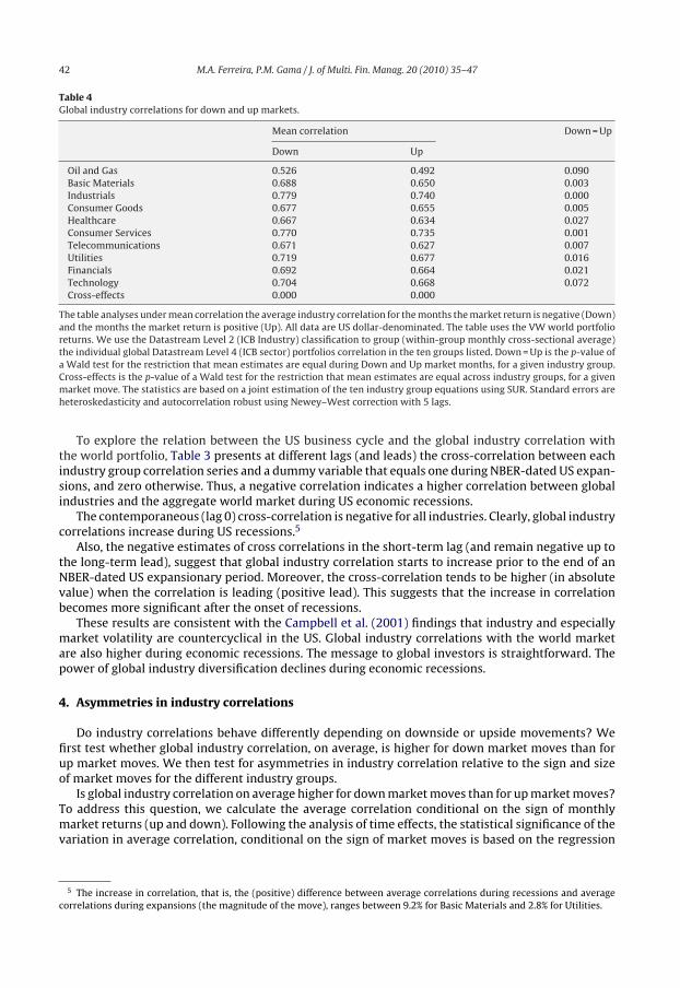
Table 4Global industry correlations for down and up markets.

Mean correlation Down = Up

Down Up

Oil and Gas 0.526 0.492 0.090Basic Materials 0.688 0.650 0.003Industrials 0.779 0.740 0.000Consumer Goods 0.677 0.655 0.005Healthcare 0.667 0.634 0.027Consumer Services 0.770 0.735 0.001Telecommunications 0.671 0.627 0.007Utilities 0.719 0.677 0.016Financials 0.692 0.664 0.021Technology 0.704 0.668 0.072Cross-effects 0.000 0.000

The table analyses under mean correlation the average industry correlation for the months the market return is negative (Down)and the months the market return is positive (Up). All data are US dollar-denominated. The table uses the VW world portfolioreturns. We use the Datastream Level 2 (ICB Industry) classification to group (within-group monthly cross-sectional average)the individual global Datastream Level 4 (ICB sector) portfolios correlation in the ten groups listed. Down = Up is the p-value ofa Wald test for the restriction that mean estimates are equal during Down and Up market months, for a given industry group.Cross-effects is the p-value of a Wald test for the restriction that mean estimates are equal across industry groups, for a givenmarket move. The statistics are based on a joint estimation of the ten industry group equations using SUR. Standard errors areheteroskedasticity and autocorrelation robust using Newey–West correction with 5 lags.

To explore the relation between the US business cycle and the global industry correlation withthe world portfolio, Table 3 presents at different lags (and leads) the cross-correlation between eachindustry group correlation series and a dummy variable that equals one during NBER-dated US expan-sions, and zero otherwise. Thus, a negative correlation indicates a higher correlation between globalindustries and the aggregate world market during US economic recessions.

The contemporaneous (lag 0) cross-correlation is negative for all industries. Clearly, global industrycorrelations increase during US recessions.5

Also, the negative estimates of cross correlations in the short-term lag (and remain negative up tothe long-term lead), suggest that global industry correlation starts to increase prior to the end of anNBER-dated US expansionary period. Moreover, the cross-correlation tends to be higher (in absolutevalue) when the correlation is leading (positive lead). This suggests that the increase in correlationbecomes more significant after the onset of recessions.

These results are consistent with the Campbell et al. (2001) findings that industry and especiallymarket volatility are countercyclical in the US. Global industry correlations with the world marketare also higher during economic recessions. The message to global investors is straightforward. Thepower of global industry diversification declines during economic recessions.

4. Asymmetries in industry correlations

Do industry correlations behave differently depending on downside or upside movements? Wefirst test whether global industry correlation, on average, is higher for down market moves than forup market moves. We then test for asymmetries in industry correlation relative to the sign and sizeof market moves for the different industry groups.

Is global industry correlation on average higher for down market moves than for up market moves?To address this question, we calculate the average correlation conditional on the sign of monthlymarket returns (up and down). Following the analysis of time effects, the statistical significance of thevariation in average correlation, conditional on the sign of market moves is based on the regression

5 The increase in correlation, that is, the (positive) difference between average correlations during recessions and averagecorrelations during expansions (the magnitude of the move), ranges between 9.2% for Basic Materials and 2.8% for Utilities.


(defined for a given industry group p correlation series):

CORp,t = ˛−p I− + ˛+

p I+ + �CORp,t−1 + εp,t (3)

where CORp,t is the average correlation with the world market portfolio in month t for industry groupp; and I− (I+) is an indicator variable for the months the return is on average negative (positive). Weestimate jointly the ten equations each relating to each industry group using the seemingly unre-lated regression (SUR). We use a joint Wald �2 test on the industry effects for the null hypothesis˛−

1 = . . . = ˛−10 and ˛+

1 = . . . = ˛+10. We test for differences in the average correlation in up and down

markets using a joint test for the null hypothesis ˛−p = ˛+

p for each industry group p.Table 4 presents the results. For all industry group series, market correlation is on average higher

during markets down months relative to market up months. The increase in correlation rangesbetween 4.4 percentage points for the Telecommunications and 2.1 percentage points for the Con-sumer Goods industries, both statistically significant.

Longin and Solnik (2001) find an asymmetric relation between country portfolio correlations withthe US stock market and the (signed) threshold used to define the (signed) return exceedances. Weinvestigate the contemporaneous relation between monthly realized industry correlation and thesign and size of market returns over the entire distribution of returns. Specifically, we estimate thefollowing equation defined for a given industry group p correlation series:

CORp,t = ˛p + ı−p I−

∣∣rm,t

∣∣ + ı+p I+

∣∣rm,t

∣∣ + �pCORp,t−1 + �prm,t−1 + εp,t (4)

where CORp,t is the portfolio p industry correlation with the world market portfolio during month t,I− (I+) is an indicator variable for the months the market return is on average negative (positive), andrm,t is the market return in month t. The parameters ı−

p and ı+p measure the contemporaneous relation

between industry correlation and world portfolio returns during falling and rising months, for eachindustry group. The lagged variables are included to pick up any serial correlation in the correlationand the absolute returns series.

An asymmetric relation between correlation and returns implies a different link between corre-lation and the size of market returns in rising and falling markets. This difference could arise fromthe sign of the link (e.g., for down months the correlation increases with market returns, while in upmonths it declines), or from the size of the link (e.g., both for falling and rising markets correlationincreases with returns, but the increase is steeper for falling markets than for rising markets).

Table 5Asymmetries in global industry correlations.

Down t-Stat Up t-Stat Down = Up (p-value)

Oil and Gas 0.839 2.17 −0.555 −1.31 0.002Basic Materials 0.533 2.22 −0.547 −1.83 0.001Industrials 0.548 4.12 −0.376 −1.83 0.000Consumer Goods 0.685 3.70 −0.089 −0.41 0.002Healthcare 0.747 2.93 −0.045 −0.13 0.017Consumer Services 0.785 5.77 −0.137 −0.63 0.000Telecommunications 0.922 2.77 −0.109 −0.30 0.004Utilities 0.324 0.92 −0.584 −1.83 0.013Financials 0.609 3.19 −0.100 −0.44 0.001Technology 0.797 3.56 0.268 0.94 0.072Cross-effects (p-value) 0.219 0.303

The table analyses the relationship between monthly world portfolio returns and the industry correlation series. All dataare US dollar-denominated. The table uses the VW world portfolio returns. We use the Datastream Level 2 (ICB Industry)classification to group (within-group monthly cross-sectional average) the individual global Datastream Level 4 (ICB sector)portfolios correlation in the ten groups listed. Down (Up) is the slope coefficient for the months the market returns is negative(positive). t-Stat is the t-statistic for the coefficient on the left. Down = Up is the p-value of a Wald test for the restriction thatslope estimates are equal in falling and rising markets, for a given industry group. Cross-effects is the p-value of a Wald test forthe restriction that slope estimates are equal across industry groups. The coefficient estimates and test statistics are based ona joint estimation of the ten industry group equations using SUR. Standard errors are heteroskedasticity and autocorrelationrobust using Newey–West correction with 5 lags.


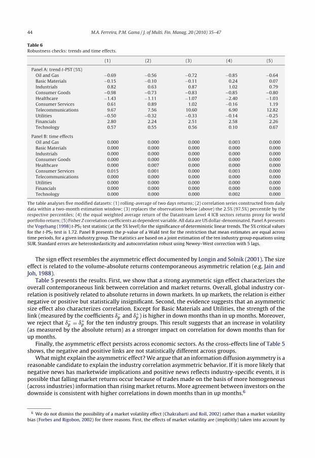
Table 6Robustness checks: trends and time effects.

(1) (2) (3) (4) (5)

Panel A: trend t-PST (5%)Oil and Gas −0.69 −0.56 −0.72 −0.85 −0.64Basic Materials −0.15 −0.10 −0.11 0.24 0.07Industrials 0.82 0.63 0.87 1.02 0.79Consumer Goods −0.98 −0.73 −0.83 −0.85 −0.80Healthcare −1.43 −1.11 −1.07 −2.40 −1.03Consumer Services 0.61 0.89 1.02 −0.16 1.19Telecommunications 9.67 7.56 10.60 6.90 12.82Utilities −0.50 −0.32 −0.33 −0.14 −0.25Financials 2.80 2.24 2.51 2.58 2.26Technology 0.57 0.55 0.56 0.10 0.67

Panel B: time effectsOil and Gas 0.000 0.000 0.000 0.003 0.000Basic Materials 0.000 0.000 0.000 0.000 0.000Industrials 0.000 0.000 0.000 0.000 0.000Consumer Goods 0.000 0.000 0.000 0.000 0.000Healthcare 0.000 0.007 0.000 0.000 0.000Consumer Services 0.015 0.001 0.000 0.003 0.000Telecommunications 0.000 0.000 0.000 0.000 0.000Utilities 0.000 0.000 0.000 0.000 0.000Financials 0.000 0.000 0.000 0.000 0.000Technology 0.000 0.000 0.000 0.002 0.000

The table analyses five modified datasets: (1) rolling-average of two days returns; (2) correlation series constructed from dailydata within a two-month estimation window; (3) replaces the observations below (above) the 2.5% (97.5%) percentile by therespective percentiles; (4) the equal weighted average return of the Datastream Level 4 ICB sectors returns proxy for worldportfolio return; (5) Fisher Z correlation coefficients as dependent variable. All data are US dollar-denominated. Panel A presentsthe Vogelsang (1998) t-PST test statistic (at the 5% level) for the significance of deterministic linear trends. The 5% critical valuesfor the t-PST test is 1.72. Panel B presents the p-value of a Wald test for the restriction that mean estimates are equal acrosstime periods, for a given industry group. The statistics are based on a joint estimation of the ten industry group equations usingSUR. Standard errors are heteroskedasticity and autocorrelation robust using Newey–West correction with 5 lags.

The sign effect resembles the asymmetric effect documented by Longin and Solnik (2001). The sizeeffect is related to the volume-absolute returns contemporaneous asymmetric relation (e.g. Jain andJoh, 1988).

Table 5 presents the results. First, we show that a strong asymmetric sign effect characterizes theoverall contemporaneous link between correlation and market returns. Overall, global industry cor-relation is positively related to absolute returns in down markets. In up markets, the relation is eithernegative or positive but statistically insignificant. Second, the evidence suggests that an asymmetricsize effect also characterizes correlation. Except for Basic Materials and Utilities, the strength of thelink (measured by the coefficients ı−

p and ı+p ) is higher in down months than in up months. Moreover,

we reject that ı−p = ı+

p for the ten industry groups. This result suggests that an increase in volatility(as measured by the absolute return) as a stronger impact on correlation for down months than forup months.

Finally, the asymmetric effect persists across economic sectors. As the cross-effects line of Table 5shows, the negative and positive links are not statistically different across groups.

What might explain the asymmetric effect? We argue that an information diffusion asymmetry is areasonable candidate to explain the industry correlation asymmetric behavior. If it is more likely thatnegative news has marketwide implications and positive news reflects industry-specific events, it ispossible that falling market returns occur because of trades made on the basis of more homogeneous(across industries) information than rising market returns. More agreement between investors on thedownside is consistent with higher correlations in down months than in up months.6

6 We do not dismiss the possibility of a market volatility effect (Chakrabarti and Roll, 2002) rather than a market volatilitybias (Forbes and Rigobon, 2002) for three reasons. First, the effects of market volatility are (implicitly) taken into account by


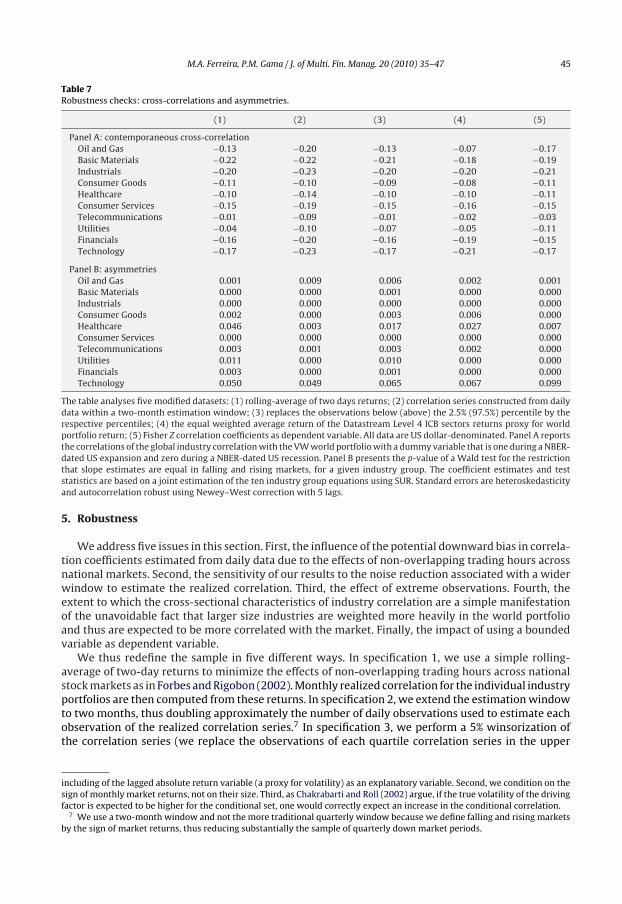
Table 7Robustness checks: cross-correlations and asymmetries.

(1) (2) (3) (4) (5)

Panel A: contemporaneous cross-correlationOil and Gas −0.13 −0.20 −0.13 −0.07 −0.17Basic Materials −0.22 −0.22 −0.21 −0.18 −0.19Industrials −0.20 −0.23 −0.20 −0.20 −0.21Consumer Goods −0.11 −0.10 −0.09 −0.08 −0.11Healthcare −0.10 −0.14 −0.10 −0.10 −0.11Consumer Services −0.15 −0.19 −0.15 −0.16 −0.15Telecommunications −0.01 −0.09 −0.01 −0.02 −0.03Utilities −0.04 −0.10 −0.07 −0.05 −0.11Financials −0.16 −0.20 −0.16 −0.19 −0.15Technology −0.17 −0.23 −0.17 −0.21 −0.17

Panel B: asymmetriesOil and Gas 0.001 0.009 0.006 0.002 0.001Basic Materials 0.000 0.000 0.001 0.000 0.000Industrials 0.000 0.000 0.000 0.000 0.000Consumer Goods 0.002 0.000 0.003 0.006 0.000Healthcare 0.046 0.003 0.017 0.027 0.007Consumer Services 0.000 0.000 0.000 0.000 0.000Telecommunications 0.003 0.001 0.003 0.002 0.000Utilities 0.011 0.000 0.010 0.000 0.000Financials 0.003 0.000 0.001 0.000 0.000Technology 0.050 0.049 0.065 0.067 0.099

The table analyses five modified datasets: (1) rolling-average of two days returns; (2) correlation series constructed from dailydata within a two-month estimation window; (3) replaces the observations below (above) the 2.5% (97.5%) percentile by therespective percentiles; (4) the equal weighted average return of the Datastream Level 4 ICB sectors returns proxy for worldportfolio return; (5) Fisher Z correlation coefficients as dependent variable. All data are US dollar-denominated. Panel A reportsthe correlations of the global industry correlation with the VW world portfolio with a dummy variable that is one during a NBER-dated US expansion and zero during a NBER-dated US recession. Panel B presents the p-value of a Wald test for the restrictionthat slope estimates are equal in falling and rising markets, for a given industry group. The coefficient estimates and teststatistics are based on a joint estimation of the ten industry group equations using SUR. Standard errors are heteroskedasticityand autocorrelation robust using Newey–West correction with 5 lags.

5. Robustness

We address five issues in this section. First, the influence of the potential downward bias in correla-tion coefficients estimated from daily data due to the effects of non-overlapping trading hours acrossnational markets. Second, the sensitivity of our results to the noise reduction associated with a widerwindow to estimate the realized correlation. Third, the effect of extreme observations. Fourth, theextent to which the cross-sectional characteristics of industry correlation are a simple manifestationof the unavoidable fact that larger size industries are weighted more heavily in the world portfolioand thus are expected to be more correlated with the market. Finally, the impact of using a boundedvariable as dependent variable.

We thus redefine the sample in five different ways. In specification 1, we use a simple rolling-average of two-day returns to minimize the effects of non-overlapping trading hours across nationalstock markets as in Forbes and Rigobon (2002). Monthly realized correlation for the individual industryportfolios are then computed from these returns. In specification 2, we extend the estimation windowto two months, thus doubling approximately the number of daily observations used to estimate eachobservation of the realized correlation series.7 In specification 3, we perform a 5% winsorization ofthe correlation series (we replace the observations of each quartile correlation series in the upper

including of the lagged absolute return variable (a proxy for volatility) as an explanatory variable. Second, we condition on thesign of monthly market returns, not on their size. Third, as Chakrabarti and Roll (2002) argue, if the true volatility of the drivingfactor is expected to be higher for the conditional set, one would correctly expect an increase in the conditional correlation.

7 We use a two-month window and not the more traditional quarterly window because we define falling and rising marketsby the sign of market returns, thus reducing substantially the sample of quarterly down market periods.


(lower) 2.5% percentiles by the 97.5% (2.5%) percentile). This procedure decreases the influence of the(extreme) observations, but leaves them as important upward or downward moves in correlation.Specification 4 uses the equal weighted average return of the Datastream Level 4 sectors returnsto proxy for world portfolio return. Finally, specification 5 uses Fisher Z correlation coefficients asdependent variable.8

Results are presented in Tables 6 and 7. Panel A (Panel B) of Table 6 replicates the trends tests(time-effects tests) in Table 1 (Table 2). Panel A (Panel B) of Table 7 replicates the contemporaneouscross correlations (asymmetric tests) of Table 3 (Table 5).

A strong message emerges. The key findings remain unaffected. In whole specifications, the industrygroups with significant trend coefficients remain the same (Telecommunications and Financials). Also,long-term (60-month) time effects characterize the behavior of industry correlation. Contemporane-ous (lag) negative cross correlations with dummy for NBER-dated expansions documents the increasein correlation during the downturns of US Business cycles. Finally, the nature of the link betweencorrelation and returns is different for down and up months, an evidence of correlation asymmetryrelative to sign and size of market returns.

6. Conclusion

Our investigation of the time series of realized correlations between global industries and theworld market reveals that global industry correlations fluctuate over time, but there is no significantlong-term trend for most industries (the exceptions are Telecommunications and Financials). Globalindustry correlations are countercyclical. They are, moreover, higher for downside moves than forupside moves. Correlation asymmetry is pervasive across industries.

The characterization of global industry correlation structure yields both reassuring and disturbinginformation for global equity investors. On the one hand, our results confirm, for industry portfolios,two features that characterize cross-country correlations. Industries are more correlated in fallingmarkets than in rising markets, and industry correlation is positively related to market volatility. Dur-ing market turmoil, global industry diversification is less able to reduce portfolio risk. Also unfavorableis the evidence that the link between correlation and volatility is stronger in rising markets than infalling markets. Thus, the negative effects for portfolio diversification of the increase in volatility aremost pervasive during up rather than down markets.

Yet industry correlations do not show a systematic increase over time, and the late 1990s werecharacterized by low correlations. Thus, industry portfolios constitute an interesting dimension forinternational diversification, as opposed to the increasingly correlated country portfolios.

References

Andersen, T., Bollerslev, T., Diebold, F., Ebens, H., 2001. The distribution of realized stock return volatility. Journal of FinancialEconomics 61, 43–76.

Ang, A., Chen, J., 2002. Asymmetric correlations of equity portfolios. Journal of Financial Economics 63, 443–494.Bekaert, G., Hodrick, R., Zhang, X., 2009. International stock return comovements. Journal of Finance 64, 2591–2626.Campbell, J., Lettau, M., Malkiel, B., Xu, Y., 2001. Have individual stocks become more volatile? An empirical exploration of

idiosyncratic risk. Journal of Finance 56, 1–43.Cavaglia, S., Diermeirer, J., Moroz, V., Zordo, S., 2004. Investing in global equities. Journal of Portfolio Management 30, 88–94.Chakrabarti, R., Roll, R., 2002. East Asia and Europe during the 1997 Asian collapse: a clinical study of a financial crisis. Journal

of Financial Markets 5, 1–30.DeStefano, M., 2004. Stock returns and the business cycle. The Financial Review 39, 527–547.Erb, C., Harvey, C., Viskanta, T., 1994. Forecasting international equity correlations. Financial Analysts Journal 50, 32–45.Ferreira, M., Gama, P., 2005. Have world, country and industry risks changed over time? An investigation of the volatility of

developed stock markets. Journal of Financial and Quantitative Analysis 40, 195–222.Forbes, K., Rigobon, R., 2002. No contagion, only interdependence: measuring stock market comovements. Journal of Finance

57, 2223–2261.French, K., Schwert, G., Stambaugh, R., 1987. Expected stock returns and volatility. Journal of Financial Economics 19, 3–30.

8 To conserve space only a subsample of the robustness results are presented in this section (Tables 5–8). The remainingresults are available upon request.


Heston, S., Rouwenhorst, K., 1994. Does industrial structure explain the benefits of international diversification? Journal ofFinancial Economics 36, 3–27.

Hong, Y., Tu, J., Zhou, G., 2007. Asymmetries in stock returns: statistical tests and economic evaluation. Review of FinancialStudies 20, 1547–1581.

Jain, P., Joh, G., 1988. The dependence between hourly prices and trading volume. Journal of Financial and Quantitative Analysis23, 269–283.

L’Her, J.-F., Sy, O., Tnami, M., 2002. Country, industry, and risk factor loadings in portfolio management. Journal of PortfolioManagement 28, 70–79.

Longin, F, Solnik, B., 1995. Is the correlation in international equity returns constant: 1960–1990? Journal of International Moneyand Finance 14, 3–26.

Longin, F., Solnik, B., 2001. Extreme correlation of international equity markets. Journal of Finance 56, 649–676.Solnik, B, Roulet, J., 2000. Dispersion as cross-sectional correlation. Financial Analysts Journal 56, 54–61.Solnik, B., Boucrelle, C., LeFur, Y., 1996. International market correlation and volatility. Financial Analysts Journal 52, 17–34.Vogelsang, T., 1998. Trend function hypothesis testing in the presence of serial correlation. Econometrica 66, 123–148.

contents lists available at sciencedirect journal of...

Documents