contents international journal of industrial organization

International Journal of Industrial Organization 59 (2018) 486–513

Contents lists available at ScienceDirect

International Journal of Industrial Organization

www.elsevier.com/locate/ijio

Incentives through inventory control in supply

chains

�

Zhan Qu

a , Horst Raffb , ∗, Nicolas Schmitt c a Faculty of Business and Economics, TU Dresden, Germany b Department of Economics, Kiel University, Kiel Centre for Globalization, and CESifo, Germany c Department of Economics, Simon Fraser University, Canada, and CESifo, Germany

a r t i c l e i n f o

Article history: Received 6 October 2017 Revised 22 May 2018 Accepted 4 June 2018 Available online 18 June 2018

JEL classification: L11 L12 L22 L81

Keywords: Inventory Supply chain Demand uncertainty Storable go o d Price discrimination

a b s t r a c t

The paper shows that taking inventory control out of the hands of competitive or exclusive retailers and assigning it to a manufacturer increases the value of a supply chain es- p ecially for go o ds whose demand is highly volatile. This is because doing so solves incentive distortions that arise when retailers have to allocate inventory across sales p erio ds, and thus allows for better intertemporal price discrimination. As- signing inventory control to a manufacturer is also shown to have effects on total inventory and social welfare.

© 2018 Elsevier B.V. All rights reserved.

� We would like to thank an anonymous referee for very helpful comments and suggestions. We are grateful for the financial support received from the Social Sciences and Humanities Research Council of Canada. Corresponding author: Horst Raff, Department of Economics, Kiel University, 24118 Kiel, Germany. ∗ Corresponding author.

E-mail address: [email protected] (H. Raff).

https://doi.org/10.1016/j.ijindorg.2018.06.001 0167-7187/ © 2018 Elsevier B.V. All rights reserved.

https://doi.org/10.1016/j.ijindorg.2018.06.001

http://www.ScienceDirect.com

http://www.elsevier.com/locate/ijio

http://crossmark.crossref.org/dialog/?doi=10.1016/j.ijindorg.2018.06.001&domain=pdf

mailto:[email protected]


Z. Qu et al. / International Journal of Industrial Organization 59 (2018) 486–513 487

1

s

g

p

A

t

H

v

a

c

S

c

g

t

w

s

e

t

t

t

C

w

t

O

w

p

fl

s

c

w

A

c

i

2

o

w

m

. Introduction

The optimal control of inventory is one of the greatest challenges faced by firms in aupply chain. Consider, for instance, a supply chain, in which a manufacturer distributeso o ds through retailers and the need to hold inventory arises, b ecause go o ds have to bero duced b efore the state of demand is known and sales to consumers can take place. key problem in this setting, as explained by Krishnan and Winter (2007) , is that

he manufacturer’s and retailers’ incentives to hold inventory are generally not aligned.ence the challenge is how to solve such incentive problems so that the supply chain’salue can be maximized.

In the current paper, we examine the incentives that arise when inventory has to bello cated intertemp orally, b ecause there is more than one sales p erio d, and inventoryontrol rests with either competitive retailers, an exclusive retailer, or the manufacturer.pecifically we show that there are two incentive distortions when competitive retailersontrol inventory, b oth asso ciated with multiple sales p erio ds. We also show that dele-ating inventory control to an exclusive retailer instead of competitive retailers resolveshese distortions, provided that the manufacturer uses two-part tariffs, but replaces themith two new ones, also associated with multiple sales p erio ds but sp ecific to the exclu-ive retailer. Thus, while incentives are b etter aligned b etween a manufacturer and anxclusive retailer than between a manufacturer and competitive retailers, it is only whenhe manufacturer controls inventory itself that these distortions disappear. Our analysishus indicates that, based on incentive considerations alone, there is a benefit to havinghe manufacturer control inventory rather than assigning inventory control to retailers.

The question of who in a supply chain should control inventory is important in practice.onsider, for example, O’Neill Inc., a US manufacturer of apparel and accessories forater sp orts. Pro duction takes place in Asia to take advantage of low costs. But due tohe long lead time (3 months), production has to occur well before the demand is known.’Neill allows for two types of orders from US retailers ( Cachon, 2004 ): one placedell before the selling season (with delivery guarantee), which means that retailers takeossession of the goods, control inventories and manage stocks over time in the face ofuctuating demand. The other type of order can be made on short notice during theelling season and is honored provided inventory is available in O’Neill’s distributionenter in San Diego. In this case, it is the manufacturer itself who controls inventory andho has to make sure that enough inventory is on hand to meet demand by retailers.nother example is Trek Inc., a US bicycle manufacturer, who lets its exclusive retailersontrol the inventory of some of its most popular products, but entirely controls thenventory of its high-end bicycles, for which demand is particularly uncertain ( Cachon,004 ).

More generally, we observe a broader trend to take inventory control out of the handsf retailers and pass it upstream to manufacturers or wholesalers, as evidenced by theidespread adoption of business practices, such as ‘drop shipping’, ‘inventory consign-ent’, and ‘vendor-managed inventory’. Drop-shipping is an arrangement used especially

488 Z. Qu et al. / International Journal of Industrial Organization 59 (2018) 486–513

by internet retailers, where these retailers forward buyers’ orders to a manufacturer or wholesaler who then ships the product from its own inventory directly to the buyer.Inventory consignment allows an upstream firm to own inventories held by downstream

firms, while vendor-managed inventory (VMI) allows a manufacturer or wholesaler to manage these inventories. 1 Already in 2002, 30% of internet retailers used drop shipping as their main means of order fulfillment compared with 5% of regular multi-channel retailers ( Randall et al., 2002 ).

What these examples show is that, thanks in part to advances in information andcommunication technologies, including in electronic sale and inventory tracking, it is now possible for manufacturers to control inventories in a more cost-effective way than

in earlier times when they were forced to let retailers control inventories. Hence it is nowmore important than ever to understand how the incentives to manage inventory differ when either retailers or manufacturers are in control.

To examine these incentive issues we use a standard model of a supply chain, in whicha manufacturer distributes go o ds through retailers, and go o ds have to be produced beforedemand is known; all sales are hence from inventory. The novelty is that we explicitlyfocus on the decision to allocate inventory intertemporally through a model with two sales p erio ds, and that we compare the cases where inventory is controlled either bycompetitive retailers, an exclusive retailer, or the manufacturer itself. Examining both

competitive retailers and an exclusive retailer, for which the manufacturer uses a two-part tariff, allows us not only to compare the two opposite extremes of retail market structures,namely perfect competition and monopoly, but also to focus on the cases in which thereis, at least in principle, no double marginalization and thus no ex-ante vertical pricedistortion that could obscure the incentive effect of inventory control. To keep the focusplainly on incentives through inventory control, we also abstract from any cost advantages that may favor the centralization of inventory control, such as economies of scale, costadvantages through the provision of complementary services such as transportation, and

economies of scope arising from pooling inventory control for different products. We show that two incentive distortions arise when competitive retailers control in-

ventory. The first has to do with the intertemporal allocation of inventory. Competitive retailers allocate inventory so that today’s retail price is equalized with tomorrow’s expected retail price. When retail prices in the two periods are tied to each other in thisway, they cannot adjust sufficiently to demand conditions in each p erio d, which imp edesintertemporal price discrimination.

The second problem associated with competitive retailers is that the excess inventory

they carry into p erio d two reduces the residual demand faced by the manufacturer andhence also the producer price in that p erio d. In effect, the manufacturer comp etes withthe excess inventory carried over by retailers from p erio d one. To limit the impact of

1 See Randall et al. (2006) for a recent comparison of drop shipping with the case of retailer-controlled inventory, Govindam (2013) for a survey, and also Mateen and Chatterjee (2015) . Information and commu- nication technologies also allow auctions to be used as inventory control tools.


t

s

s

d

a

s

w

t

c

s

o

a

t

p

d

a

d

b

o

fi

p

p

i

a

m

a

f

o

c

(

t

s(fJcfoaT

his inventory competition the manufacturer would have to keep shipments in p erio d onemall, but by doing so it runs the risk of losing sales due to stockouts. It is to avoid thesetockouts that the manufacturer has to ship more than would be optimal without theistortion. Next we show that, by assigning inventory control to an exclusive retailer and using

two-part tariff, the manufacturer can eliminate inventory competition, while at theame time avoiding stockouts. On this count then, the exclusive retailer’s incentiveshen it controls inventory are better aligned with the interests of the manufacturer than

hose of competitive retailers. However, having an exclusive retailer control inventoryreates two distortions of its own, so that intertemporal price discrimination is stilluboptimal. One distortion comes from the fact that the exclusive retailer does notptimally allocate inventory across periods. In particular, we show that the retailer hasn incentive to carry too much excess inventory into p erio d two and therefore to orderoo little in that p erio d. The manufacturer responds to this by raising the p erio d-onero ducer price ab ove marginal cost, which leads to a second distortion in the form ofouble marginalization. In other words, whether the retailers are competitive or exclusivend whether the manufacturer uses linear or two-part pricing, there are still verticalistortions when retailers control inventories. We show that these vertical distortionsecome worse the higher is the variance of demand. Thus, from the manufacturer’s pointf view, taking inventory control away from retailers is especially useful in markets wherenal demand is very volatile. However, while letting the manufacturer control inventory raises the overall expected

rofit of the supply chain, the effect on expected consumer surplus and social welfare de-ends on retail market structure. Expected consumer surplus and social welfare fall whennventory control is passed from competitive retailers to the manufacturer. Hence, in thebsence of major cost savings from shifting inventory control to the manufacturer, such aove should be viewed as being anticompetitive. The opposite effect on consumer surplus

nd social welfare is obtained when inventory control is transferred to the manufacturerrom an exclusive retailer.

Incentive problems in decentralized supply chains have been analyzed by the literaturen vertical control in industrial organization and by the management literature on supplyhain coordination. 2 In particular, Krishnan and Winter (2007) and Deneckere et al.1996) explain that the price system generically fails to align retailers’ incentives withhose of the manufacturer when inventory control is involved. Our model is closely related

2 See Krishnan and Winter (2012) for a synthesis of these two strands of literature. In the management cience literature, articles such as Belavina and Girotra ( 2012a, 2012b ), and Biyalogorsky and Ko enigsb erg 2010) investigate how decentralized decision-making through intermediation can improve supply chain per- ormance, or who should retain product ownership in a supply chain. More specifically related to inventory, erath et al. (2017) link product quality and inventory risks, Huh and Janakiraman (2008) show how auctions ould be used to manage inventory, and Anand et al. (2008) show how retailers can accumulate inventories or strategic reasons independently of demand uncertainty. There is also, of course, a long literature on ptimal order policies and inventory levels going back to seminal contribution of Arrow et al. (1951) . Clark nd Scarf (1960) were the first to establish an optimal inventory policy in a multi-echelon supply chain. hese papers, however, do not examine the incentive problems associated with inventory control.


to the one by Deneckere et al. (1997) , in which a manufacturer sells go o ds throughcompetitive retailers who control inventory. Unlike in our paper, inventory in Deneckere et al. perishes after one period, which implies that retailers will sell their entire inventory,even if the retail price drops to zero. It is this risk of ‘destructive competition’ thatexplains why retailers may hold too little inventory, and it is to avoid this effect that themanufacturer may want to intervene, for instance, by imposing resale price maintenance or offering buy-back policies.

By contrast, we deliberately choose to eliminate destructive competition by allowing retailers to shift unsold inventory into the second p erio d and by assuming that the de-mand shocks are sufficiently small so that the retail price never hits zero in p erio d 2.This allows us to focus on the intertemporal incentive problems associated with retailer- controlled inventory. As already mentioned above, these incentive problems imply that retail prices do not adjust optimally to demand conditions, so that intertemporal price discrimination is impeded. Moreover, competitive retailers tend to order too much inventory from the manufacturer’s point of view, which is in stark contrast to the findings byDeneckere et al. (1997) .

Another departure from Deneckere et al. is that we consider how incentives would

change if control over inventory were assigned to an exclusive retailer. In the Deneckereet al. model, having an exclusive retailer in control of inventory and imposing a two-part tariff would solve the problem of destructive competition and lead to an optimal inventory policy. In our model, by contrast, incentive problems persist even with an

exclusive retailer, meaning that intertemporal price discrimination is still not optimal. Only when the manufacturer takes control of inventory can the intertemporal allocation

distortions be eliminated in our model. However, this reduces social welfare with respect to the case where competitive retailers hold inventory. By contrast, eliminating incentive distortions in Deneckere et al. raises social welfare, as inventory rises.

Another related paper is by Krishnan and Winter (2010) . In their model a manufac-turer distributes go o ds through two retailers, and excess inventory may be carried overinto the subsequent p erio d. They show that, if inventory do es not p erish to o quickly,retailers may hold too much inventory. This is similar to the results of our paper, but theintertemporal incentive distortions leading to this result are different from ours, in part because inventory in their mo del has itself a p ositive effect on consumer demand. Theirpaper also differs from ours in other respects. For instance, Krishnan and Winter do notexamine how the incentives to hold inventory differ between competitive and exclusive retailers, and what the consequences of different inventory control arrangements are for social welfare.

Our paper is also related to the literature on intertemporal price discrimination

( Varian, 1989; Bulow, 1982; Koh, 2006; Dudine et al., 2006 ). In this literature, consumersengage in strategic behavior whether it is to delay purchases (as with durable go o ds), orto sto ckpile go o ds when consumers anticipate an (exogenous) increase in prices (as withstorable go o ds). Consumers’ strategic b ehavior is thus at the heart of results wherebya firm competes with itself (as in the Coase conjecture in the durable go o d monop oly


p

t

n

w

H

e

p

a

r

a

r

2

I

a

d

t

s

t

p

A

v

d

a

c

i

a

e

c

t

trgttt

roblem). By dealing with intertemporal incentives associated with inventory control athe firm level, we do not need consumer strategic behavior, and our analysis thus doesot depend on such consumers. The products we have in mind are thus those like toys forhich there are typically very few well-defined p erio ds of high but uncertain sales (likealloween and Christmas). Also relevant are products like apparel, sporting goods, andven certain types of automobiles for which manufacturers p erio dically intro duce newroducts or models and discontinue old ones. The rest of the paper is organized as follows. In Sections 2 –4 , we present our model

nd derive the equilibrium if inventory is controlled by competitive retailers, an exclusiveetailer and the manufacturer, respectively. Section 5 discusses some implications of thenalysis, Section 6 contains conclusions, and the App endix collects the pro ofs of ouresults.

. The model and benchmark case

Consider a supply chain consisting of a manufacturer selling go o ds through retailers.n the b enchmark mo del, we follow Deneckere et al. (1997) by assuming that retailersre p erfectly comp etitive. 3 Retailers have to order and take possession of go o ds b eforeemand is known. Once demand has been revealed, the retailers sell to consumers. Thus,he retailers hold inventories, that is to say the units received from the manufacturer andtored before they are sold.

We deviate from Deneckere et al. (1997) by assuming that there are two sales p erio ds, = 1 , 2 , which means that the product under consideration loses its value after two erio ds. Demand at time t = 1 , 2 is given by the linear inverse demand function: p t = − s t + ε t , where p t is the retail price and s t denotes final sales in p erio d t . The randomariables ε t ∈ [ −d, d ] are intertemporally independent and uniformly distributed withensity 1/2 d . 4 We keep the assumptions about the production and distribution technologies as simple

s possible. The manufacturer incurs a constant unit cost of production c . The marginalost of retailers is normalized to zero, as is the cost of holding inventory, and theres no discounting between periods. All market participants are risk neutral. We alsossume A > c , and that the demand shock is not too big, d ≤ d̄ = min

[ c √

2 , A −c

2

] so that

quilibrium prices and sales in each p erio d are always non-negative in all the environmentsonsidered in the analysis (see App endix 6 ). Imp ortantly, the latter assumption implieshat, in equilibrium, all inventory remaining in p erio d 2 is sold at a p ositive price and

3 The assumption of perfectly competitive retailers is not overly restrictive in the sense that one can view

he competitive outcome as the limit of a sequential game among oligopolistic retailers as the number of etailers gets large. In stage one retailers order inventory, each taking the quantity of the other retailers as iven (Cournot competition). In stage two, after observing the true realization of demand, retailers simul- aneously announce retail prices. The outcome of the subgame perfect equilibrium of this game converges o the perfectly competitive outcome as the number of retailers goes to infinity. See Tirole (1988) , ch. 5 and he references cited there for the relevant convergence results. 4 We explain in an online Appendix how robust our results are to relaxing these assumptions.


thus that destructive competition ( Deneckere et al., 1996; 1997 ), another source of (static)incentive problems arising from retailer controlled inventory, is assumed away. Allowing for the possibility of destructive competition and/or more complicated cost structures would obscure the intertemporal incentive issues that we focus on.

The order of moves can now be summarized as follows. At the beginning of p erio d 1,the manufacturer announces a producer price P 1 , retailers order and take possession of q 1 units of go o ds b efore demand in p erio d 1 is known; then p erio d-one demand is revealedand the retailers sell s 1 ≤ q 1 in p erio d 1, holding unsold units in inventory for p erio d 2.In p erio d 2, the manufacturer sets pro ducer price P 2 , and retailers order quantity q 2 ,again before demand is known. Demand in period 2 is then revealed and retailers sells 2 ≤ q 2 + ( q 1 − s 1 ) .

Now consider p erio d 2. The retailers sell all of the products on hand because theyhave already paid for these go o ds and, for d ≤ d̄ , the retail price is positive. Hences 2 = q 2 + ( q 1 − s 1 ) : sales in p erio d 2 correspond to the sum of the excess inventory carriedover from p erio d 1 and the quantity ordered in p erio d 2. Since retailers must order beforethe demand in that p erio d is known, comp etitive retailers order go o ds in p erio d 2 untilthe expected consumer price in period 2 equals the producer price P 2 , and thus untilE ( A − s 2 + ε 2 ) = A − q 2 − ( q 1 − s 1 ) = P 2 .

The manufacturer cho oses P 2 , resp ectively q 2 , to maximize its p erio d-2 profit ( P 2 −c ) q 2 . This profit is maximized for q 2 = ( A − c − ( q 1 − s 1 ) ) / 2 or P 2 such that:

P 2 = E( p 2 ) =

{

A + c 2 − ( q 1 −s 1 )

2 if s 1 < q 1 , A + c

2 otherwise. (1)

Thus, if all units ordered in p erio d 1 are sold in that p erio d ( s 1 = q 1 ) , the manufacturersets the producer price in p erio d 2 equal to the static monopoly price. But if retailerscarry excess inventory into p erio d 2 ( s 1 < q 1 ), the manufacturer is forced to reduce itspro ducer price b elow the static monop oly price. This price effect, which we refer toas inventory competition , can be viewed as a vertical distortion coming directly fromdelegating inventory control to retailers. This distortion has implications for p erio d 1.To see this, it suffices to recognize that orders in p erio d 1, q 1 , are critical to determinewhether or not there is inventory competition in period 2, since the bigger is q 1 , the morelikely it is that excess inventory will be passed on to period 2. Obviously the manufacturerwants to take into account how retailers make their choices in p erio d 1 to determine theoptimal producer price in that period, P 1 .

Turning then to p erio d 1, once the demand in that p erio d has been revealed, retailerssell as long as the realized retail price, p 1 ( ε 1 ), is greater than or equal to the expectedretail price in p erio d 2. Hence, sales in p erio d 1, s 1 , are determined by the condition:

p 1 ( ε 1 ) = E( p 2 ) . (2)


F

p

d

p

r

w

G

r

r

t

b

b

t

s

t

q

o

c

P

t

2

q

P

r

a

or s 1 < q 1 , this implies that p 1 ( ε 1 ) = A − s 1 + ε 1 =

A + c −q 1 + s 1 2 = E 2 ( p 2 ) . By linking

rices in the two p erio ds in this fashion comp etitive retailers imp ede intertemp oral priceiscrimination. In fact, optimal price discrimination would have required a level of first- erio d sales that equates the marginal revenue in p erio d 1 to the expected marginalevenue in p erio d 2. 5 Given the distortion inherent in (2) , it follows that

s 1 =

{

A −c +2 ε 1 3 +

1 3 q 1 < q 1 if ε 1 < ˆ ε 1 ,

q 1 otherwise, (3)

here ˆ ε 1 = q 1 −

A − c

2 . (4)

iven q 1 , (3) offers two possible outcomes for s 1 . Either s 1 < q 1 if there is a relatively lowealization of demand leading to inventory competition in p erio d 2, or else, if there is aelatively high realization of demand in p erio d 1, s 1 = q 1 and retailers stock out so thathey do not carry any excess inventory into p erio d 2.

If inventory competition is a problem for the manufacturer, having retailers stock outy selling in p erio d 1 all the units ordered is also a problem, since it implies that sales areeing lost. It is obvious from (4) that the level of q 1 determines the value of ˆ ε 1 and thushe range of demand realizations leading either to inventory competition in p erio d 2 ortockout in period 1. The manufacturer has just one tool at its disposal, P 1 or equivalentlyhe choice of q 1 , to balance these two effects. Formally, this trade-off is solved by choosing 1 to maximize the manufacturer’s expected profit E { ( P 1 − c ) q 1 + ( P 2 ( q 1 ) − c ) q 2 ( q 1 ) } .

The following proposition shows how the manufacturer optimally deals with this trade-ff, where the superscript ‘ cr ’ denotes the expected equilibrium values in the case ofompetitive retailers:

roposition 1. Suppose inventory is controlled by competitive retailers. The manufac-urer, facing a trade-off between lost sales in period 1 and inventory competition in period, chooses to sell in period 1 more than the one-period static monopoly output, namely

cr 1 =

( A −c ) 2 +

d 5 , and to incur a 40% probability that retailers stock out.

ro of. See App endix . �

To understand the intuition behind the manufacturer’s choice of q 1 , it is useful toewrite the manufacturer’s first-order condition derived in the Appendix (see Eq. (A.5) )s follows:

2 ( A − c − 2 q 1 ) + 7 d ∫

ˆ ε 1

(A − c − 2 q 1 +

8 7 ε 1

)1 2 d dε 1 = 0 . (5)

5 We will come back to this distortion in the next sections.


The first term represents the maximization condition for expected profits assuming there is no possibility of a stockout. This term would be equal to zero at the static monopolyoutput of q 1 = ( A − c ) / 2 . That is, if there were no possibility of a stockout, the manu-facturer would simply deliver the unconstrained optimal monopoly quantity for p erio d

1, because retailers at least in expectation would then have no incentive to hold go o dsback for p erio d 2, which would prevent inventory competition. The second term reflectsthe adjustment in the maximization condition that has to be made to account for thepossibility of a stockout. This term implies that the static monopoly output is insuffi-cient to maximize profit. Instead, the manufacturer wants to choose a higher output inp erio d 1, thus allowing some inventory competition in order to reduce the probability ofa stockout. The probability of a stockout being less than 50% is then the by-product ofshipping more than the static monopoly quantity in period 1.

The consequence of allowing some inventory competition in period 2 is not only that the manufacturer sets a relatively low P 2 , but also that it ships a relatively small expectedquantity in that p erio d, one that is smaller than the static monopoly output. Overall, weobtain the following result for the manufacturer’s expected total output and total profit:

Proposition 2. Suppose inventory is controlled by competitive retailers. The manufacturer’s total expected equilibrium output, E( q cr ) ≡ q cr 1 + E( q cr 2 ) = ( A − c ) +

2 d 25 , and ex-

pected equilibrium profit, E ( Πcr ) =

( A −c ) 2 2 +

d 2

25 , exceed the sum over two periods of thestatic monopoly output, respectively static monopoly profit.

Pro of. See App endix . �

Notice that the equilibrium profit earned by the manufacturer is greater, namely by

d

2 /25, than the expected static monopoly profit over two p erio ds. This comes from thefact that, after observing ε 1 , any excess inventory can be carried over to p erio d 2, and thequantity ordered in p erio d 2 can also be adjusted. But, as we showed in this section, thereare two reasons why this profit is still lower than it could be. First, in order to lower theprobability of a stockout, the manufacturer ships a larger quantity in p erio d 1. As willbecome evident below, this leads to an overall quantity that is too large to maximize thesupply chain’s value. Second, competitive retailers prevent optimal intertemporal price discrimination because they choose first-period sales to equalize the retail price in period

1 with the expected retail price in p erio d 2. In the next section, we contrast this casewith the one where the manufacturer uses an exclusive retailer to control inventory.

3. Inventory control by an exclusive retailer

Consider now the case of a manufacturer selling to an exclusive retailer and using two-part tariffs. Thus, the manufacturer sets a producer price, P t , and a fixed payment (or


t

Ib

s

t

g

r

m

p

m

t

c

t

t

i

p

q

t

s

a

t

w

c

p

b

f

P

m

t

t

p

ransfer), T t , in each p erio d t = 1 , 2 . 6 This case is interesting for the following reasons.f the manufacturer used linear pricing, it would face qualitatively the same trade-offetween inventory competition in period 2 and lost sales due to stockouts in p erio d 1,imply because it would still have only one instrument at its disposal to deal with thisrade-off. A two-part tariff, by providing an additional instrument to the manufacturer,ives it more scope to resolve the inventory competition problem without running theisk of stockouts. In addition, two-part tariffs imply that, in principle, there is no doublearginalization when it deals with an exclusive retailer and that the entire expectedrofit generated by the supply chain goes to the manufacturer. It also implies that theanufacturer has nothing to gain from having more than one retailer. Thus, one re-

ailer controlling inventory represents the opp osite extreme with resp ect to dealing withompetitive retailers. We want to show that a vertical distortion is still present.

The timing of moves is as before, except that the manufacturer now sets a two-partariff each p erio d. That is, at the b eginning of p erio d 1, the manufacturer sets a two-partariff ( P 1 , T 1 ), the exclusive retailer orders and takes possession of quantity q 1 . Demandn p erio d 1 is then revealed, and the retailer sells to consumers a quantity s 1 ≤ q 1 . In erio d 2, the manufacturer chooses the two-part tariff ( P 2 , T 2 ), and the retailer orders auantity q 2 . Then demand in p erio d 2 is revealed and the retailer sells s 2 ≤ q 2 + ( q 1 − s 1 ) .

The key difference with respect to the case of competitive retailers turns out to behat an exclusive retailer can guarantee itself an expected profit in p erio d 2 of at least

πout ≡ [ A − ( q 1 − s 1 ) ] ( q 1 − s 1 ) , (6)

imply by selling unsold units carried over from p erio d 1, ( q 1 − s 1 ) , and refusing anydditional orders in p erio d 2. The exclusive retailer, it is important to notice, receiveshis profit, whether or not it orders output in p erio d 2. As a result, if the manufacturerants to sell output to the retailer in p erio d 2, it has either to reduce the fixed payment itharges the retailer in p erio d 2 by the amount πout , or else to decrease its second-p erio droducer price. As it turns out, the manufacturer indeed finds it optimal to reduce the fixed payment

y πout and to set the producer price in p erio d 2 equal to marginal cost c . This has theollowing implication:

roposition 3. Suppose that inventory is controlled by an exclusive retailer, and that theanufacturer uses a two-part tariff. If the retailer orders a positive quantity in period 2,

hen the expected retail price in period 2 is equal to the static monopoly price, E( p 2 ) =A + c

2 . Hence inventory competition is eliminated.

To prove this, suppose that the excess inventory from p erio d 1 is small enough sohat q 2 > 0. The retailer’s expected profit in period 2 is then equal to ( A − q 2 − ( q 1 −

6 In principle, the manufacturer could also use two-part tariffs when it sells to competitive retailers. But erfect comp etition in retailing implies that the transfer in each case would be equal to zero in equilibrium.


s 1 ))( q 2 + ( q 1 − s 1 )) − P 2 q 2 − T 2 so that its profit-maximizing order is

q 2 =

A − P 2

2 − ( q 1 − s 1 ) > 0 , (7)

and the expected retail price is E( p 2 ) =

A + P 2 2 . To show that the manufacturer sets P 2 = c,

it suffices to derive the retailer’s expected profit in period 2,

E ( π2 ) = E( p 2 ) s 2 − P 2 q 2 − T 2 (8)

=

( A − P 2 ) 2

4 + P 2 ( q 1 − s 1 ) − T 2 , (9)

and then to find the manufacturer’s optimal two-part tariff ( T 2 , P 2 ) such that T 2 extractsthe retailer’s expected period-2 profit net of the retailer’s outside option, πout , and P 2 maximizes

( P 2 − c ) q 2 ( P 2 ) + E ( π2 ) − πout (10)

= ( P 2 − c ) [A − P 2

2 − ( q 1 − s 1 ) ]

+

( A − P 2 ) 2

4 + P 2 ( q 1 − s 1 ) − πout .

From the corresponding first-order condition, we obtain the manufacturer’s optimal choice P 2 = c . Therefore the manufacturer’s expected profit in p erio d 2 conditional onq 2 > 0 is

E ( Π2 ) =

( A − c ) 2

4 + c ( q 1 − s 1 ) − πout

=

( A − c ) 2

4 + [ c −A + ( q 1 − s 1 ) ] ( q 1 − s 1 ) .

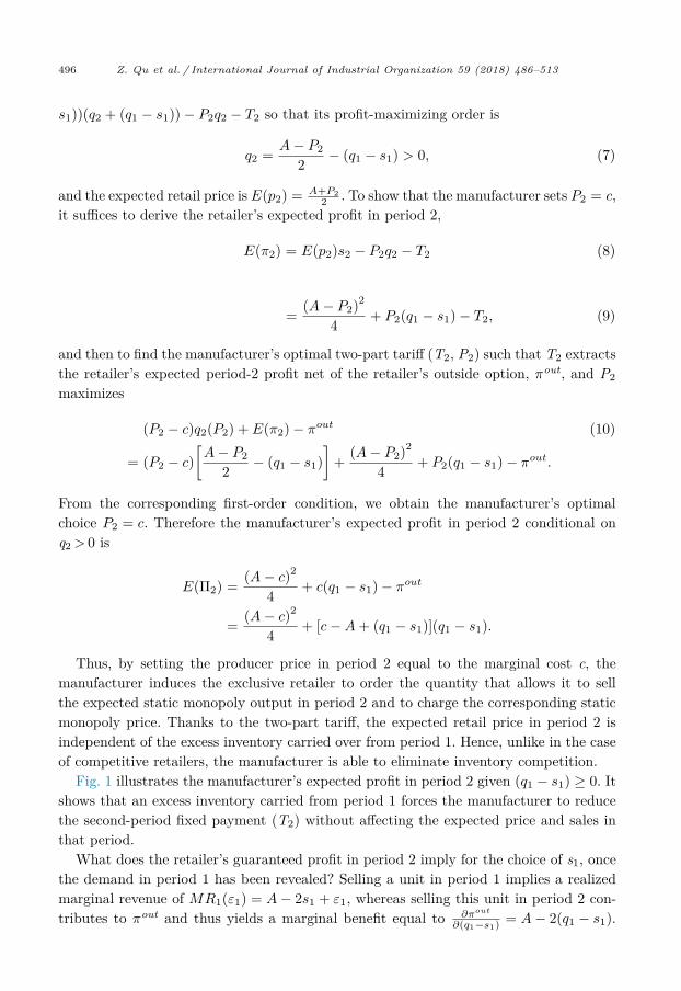
Thus, by setting the producer price in period 2 equal to the marginal cost c , themanufacturer induces the exclusive retailer to order the quantity that allows it to sellthe expected static monopoly output in period 2 and to charge the corresponding static monopoly price. Thanks to the two-part tariff, the expected retail price in p erio d 2 isindependent of the excess inventory carried over from p erio d 1. Hence, unlike in the caseof competitive retailers, the manufacturer is able to eliminate inventory competition.

Fig. 1 illustrates the manufacturer’s expected profit in period 2 given ( q 1 − s 1 ) ≥ 0 . Itshows that an excess inventory carried from p erio d 1 forces the manufacturer to reducethe second-p erio d fixed payment ( T 2 ) without affecting the expected price and sales inthat p erio d.

What does the retailer’s guaranteed profit in p erio d 2 imply for the choice of s 1 , oncethe demand in p erio d 1 has been revealed? Selling a unit in period 1 implies a realizedmarginal revenue of M R 1 ( ε 1 ) = A − 2 s 1 + ε 1 , whereas selling this unit in p erio d 2 con-tributes to πout and thus yields a marginal benefit equal to ∂πout

∂( q 1 −s 1 ) = A − 2 ( q 1 − s 1 ) .


Fig. 1. Manufacturer’s Expected Profit - Period 2.

H

W

T

t

t

H

i

w

t

p

P

m

t

ence the retailer chooses s 1 so that

M R 1 ( ε 1 ) =

∂πout

∂( q 1 − s 1 ) . (11)

e can solve (11) to obtain

s 1 =

q 1 2 +

ε 1 4 . (12)

his shows that, because the retailer values excess inventory, it chooses to sell only halfhe quantity ordered in p erio d 1 (plus ε 1 /4 which may b e p ositive or negative).

The manufacturer selects the optimal two-part tariff ( P 1 , T 1 ) such that T 1 extractshe retailer’s total expected profit in period 1 and P 1 maximizes

( P 1 − c ) q 1 ( P 1 ) + T 1 ( P 1 ) +

∫ d

ˆ ε 1 ( P 1 ) Π2

1 2 d dε 1 . (13)

ence the manufacturer takes into account how its choice of P 1 affects its expected profitn p erio d 2 understanding that this exp ected profit dep ends on the retailer’s re-orderinghich occurs only if the demand shock in period 1 is bigger than the threshold ˆ ε 1 . Using

he superscript ‘ ex ’ to denote equilibrium values in the case of an exclusive retailer, werove:

roposition 4. Suppose inventory is controlled by an exclusive retailer. In period 1, theanufacturer optimal ly sel ls q ex 1 = A − c −

( 3 2 −

√

2 )d . This shipment is sufficiently large

o avoid any possibility of stockout.



To understand this proposition, it is useful to rewrite the manufacturer’s first-order condition coming from (13) (see also Eq. (A.13) in Appendix 3 ) as:

−( P 1 − c ) − 1 2

d ∫

−( 2 P 1 −2 c )

(c − P 1 −

ε 1 2

) 1 2 d dε 1 = 0 . (14)

When the retailer has no opportunity to re-order in p erio d 2, the first-order conditionreduces to the first term with the manufacturer setting P 1 = c . As a result, q 1 = A − c sothat the retailer orders twice the static monopoly output in p erio d 1. The second termreflects the effect of P 1 on the manufacturer’s expected profit when the retailer has anopportunity to re-order and thus when q 2 > 0. In the Appendix , we formally show thatq 2 > 0 requires ε 1 > ˆ ε 1 = −2( P 1 − c ) and that it is this term that leads to P 1 exceedingc . The intuition is clear. Raising P 1 decreases T 1 but increases the probability that thep erio d-2 order is positive, thereby raising the manufacturer’s expected profit in that p erio d. We show that even with P 1 exceeding c the retailer is still left with an incentiveto place a large enough order in p erio d 1 to avoid a stockout.

Now that we have determined how much the manufacturer ships in p erio d 1, we candetermine how much is shipped in equilibrium in period 2. Given sales in period 1 equalto s 1 =

q 1 2 +

ε 1 4 and desired expected sales in period 2 equal to s 2 =

A −c 2 , we have

q 2 = s 2 − ( q 1 − s 1 )

=

A − c

2 − ( q 1 − s 1 )

=

1 4

[ (3 − 2

√

2 )d + ε 1

] . (15)

It follows that the retailer orders go o ds in p erio d 2 ( q 2 > 0) only if demand in the firstp erio d is large enough such that ε 1 > ˆ ε 1 = −

(3 − 2

√

2 )d . If ε 1 < ˆ ε 1 , the retailer does

not order any go o ds in p erio d 2 and is content with the initial order. Accordingly, theexp ected second-p erio d shipment by the manufacturer is

E ( q ex 2 ) =

d ∫

−( 3 −2 √

2 ) d

[ (3 − 2

√

2 )d + ε 1

4

]

1 2 d dε 1 =

(3 − 2

√

2 )

2 d. (16)

The manufacturer’s total expected output and total expected profit can now be computed. They are as follows:

Proposition 5. Suppose inventory is controlled by an exclusive retailer. The manufacturer’s equilibrium output, E ( q ex ) ≡ q ex 1 + E( q ex 2 ) = A − c , is the same as the sum


o

E

P

c

w

i

t

i

h

t

i

r

o

b

m

H

s

c

c

p

c

m

4

c

c

i

t

c

d

aicr

ver two periods of the static monopoly outputs, and the expected equilibrium profit, ( Πex ) =

( A −c ) 2 2 +

(4 √

2 −5 12

)d 2 , exceeds the sum of the static monopoly profits.

ro of. See App endix . �

A comparison of the expected profit with that in the case of competitive retailersonfirms that an exclusive retailer’s incentives to manage inventory are better alignedith the manufacturer’s interest than those of competitive retailers. The reasons are that

nventory competition is eliminated without incurring the risk of a stockout, and thathe exclusive retailer is better at allocating inventory across p erio ds, which improvesntertemporal price discrimination. 7

However, even if there is no longer any inventory competition and the exclusive retailerelps improve intertemporal price discrimination, there is still a distortion induced byhe retailer’s incentive to carry too much excess inventory into p erio d 2 and thus toncrease πout . We can call this an inventory rent distortion . To see how it comes about,ecall from (11) that the retailer chooses s 1 to equate the marginal revenue from sellingne more unit in p erio d 1, MR 1 ( ε 1 ) with the marginal increase in the outside profit,∂πout

∂( q 1 −s 1 ) . What the retailer should be doing to maximize the chain’s total profit, as wille shown formally in the next section, is instead to choose s 1 such that revenue on thearginal unit sold in p erio d 1 is equal to the replacement cost of this unit, namely c .ence a distortion arises as soon as ∂πout

∂( q 1 −s 1 ) � = c . In particular, using (12) , it is easy toee that a high demand shock ( ε 1 > ˆ ε 1 ) implies ∂πout

∂( q 1 −s 1 ) > c ; this means that the retailerarries too much inventory into p erio d 2, b ecause it values a unit of excess inventoryarried into p erio d 2 at more than the producer price at which it could buy this unit in erio d 2, namely c . It is to reduce this distortion that the manufacturer raises P 1 above . While this increases the manufacturer’s expected total profit, the resulting doublearginalization causes a deadweight loss.

. Inventory control by the manufacturer

The previous section shows that a distortion still exists when an exclusive retailerontrols inventory because of the value that the retailer attaches to excess inventoryarried into p erio d 2. What then is the outcome if the manufacturer controls inventorytself, either in the sense that it is vertically integrated into retailing, or in the sensehat it lets competitive retailers set retail prices but controls the quantity shipped toonsumers each p erio d as would b e the case, for instance, with the business practicesiscussed in the introduction, namely drop shipping, inventory consignment or vendor-

7 Notice, however, that inducing the retailer to allocate inventory b etter b etween p erio ds requires shipping large quantity in p erio d 1 and letting the retailer carry large excess inventory into p erio d 2. This solution s obviously facilitated by our assumption that there are no costs of holding inventory. Introducing such osts would reduce the advantage of having an exclusive retailer control inventory relative to competitive etailers.


managed inventory. Of course, pro duction still needs to b e committed b efore the demandis known, but q t should no longer be interpreted as a retail order but rather as themanufacturer’s production ready for sale before the demand is revealed in each p erio dt = 1 , 2 .

Consider p erio d 2. Given that d ≤ d̄ , retail sales in p erio d 2 equal s 2 = q 2 + ( q 1 − s 1 ) ,the expected profit of the manufacturer is ( A − q 2 − ( q 1 − s 1 ))( q 2 + ( q 1 − s 1 )) − cq 2 , andthe manufacturer’s optimal production is

q 2 =

A − c

2 − ( q 1 − s 1 ) . (17)

This implies that s 2 =

A −c 2 and the expected retail price is p 2 =

A + c 2 whether or not

there is excess inventory at the end of p erio d 1. The manufacturer’s expected profit inp erio d 2 is

E ( Π2 ) =

( A − c ) 2

4 + c ( q 1 − s 1 ) , (18)

where the unsold units carried over from p erio d 1 are valued at their replacement cost c .In p erio d 1 after ε 1 has b een revealed, the manufacturer’s marginal revenue is equal

to M R 1 ( ε 1 ) = A − 2 s 1 + ε 1 , and it must decide how to allocate units across p erio ds. Weconsider the case where q 2 > 0, which is satisfied for d ≤ d̄ . The manufacturer’s optimalchoice of s 1 is given by the intertemporal optimization condition

M R 1 ( ε 1 ) = c, (19)

which states that the manufacturer values the marginal unit sold in p erio d 1 at itsreplacement cost. Hence

s 1 =

A − c

2 +

ε 1 2 . (20)

So what is the manufacturer’s optimal choice of q 1 before observing ε 1 ? By producingin p erio d 1 a quantity

q m

1 =

A − c + d

2 , (21)

and in p erio d 2, after observing ε 1 , producing a quantity

q m

2 =

A − c

2 − ( q 1 − s 1 ) (22)

=

A − c

2 − d − ε 1 2 ,

the manufacturer can make sure that it has enough inventory on hand to realize theoptimal s 1 and s 2 for any realization of ε 1 . This way the manufacturer can achieve amaximal total expected profit given by

E ( Πm ) =

∫ d

−d

( A − c + ε 1 ) 2

4 1 2 d dε 1 +

( A − c ) 2

4 , (23)


P

e

t

e

s

i

e

a

r

d

5

w

r

t

m

m

i

c

b

f

P

i

r

e

c

c

p

t

p

=

( A − c ) 2

2 +

d 2

12 . (24)

We may hence state:

roposition 6. Suppose inventory is controlled by the manufacturer. The manufacturer’squilibrium output, E ( q m ) = q m

1 + E( q m

2 ) = A − c , is equal to the sum over two periods ofhe static monopoly outputs, and the expected equilibrium profit, E ( Πm ) =

( A −c ) 2 2 +

d 2

12 ,

xceeds the sum of the static monopoly profits.

The advantage of having the manufacturer in control of inventory relative to an exclu-ive retailer comes directly from the intertemp oral allo cation condition (19) . By equat-ng marginal revenue in p erio d 1 with the replacement cost (and thus implicitly withxpected marginal revenue in p erio d 2), the manufacturer can ensure that retail pricesdjust optimally to differences in demand conditions across p erio ds induced by differentealizations of ε 1 . That is, only in the case of manufacturer-controlled inventory can priceiscrimination across p erio ds b e optimal.

. Implications

We can now derive several implications from the analysis by comparing the equilibriumhere competitive retailers control inventories with the equilibria where an exclusiveetailer, respectively the manufacturer does. The first implication concerns the incentiveso take inventory control away from competitive or exclusive retailers and assign it to theanufacturer. A comparison of Propositions 2, 5 and 6 shows, not surprisingly, that theanufacturer’s profit is highest when it controls inventory itself, second highest when

nventory control rests with an exclusive retailer and lowest when competitive retailersontrol inventory. More interestingly, the difference in profits between these scenariosecomes greater the greater is the variance of demand, and thus d . We hence obtain theollowing result:

roposition 7. The greater is the variance of demand (and thus d) the greater is thencentive to let inventory be controlled by an exclusive retailer rather than competitiveetailers and by the manufacturer rather than an exclusive retailer.

Thus, the distortions associated with having inventory controlled by competitive orxclusive retailers become greater, the greater is the variance of demand. To see why,onsider the impact of a big negative demand shock on inventory competition. In thisase, competitive retailers are likely to carry a lot of excess inventory into the second erio d, even if the manufacturer only shipped a small quantity in p erio d 1, thus exp osinghe manufacturer to inventory competition and forcing it to cut the producer price in erio d 2. In the case of a big positive demand shock, the manufacturer faces another


problem, namely that competitive retailers are likely to stock out and sales are lost. When inventory is controlled by an exclusive retailer, a comparison of the intertemporal allocation rules (11) and (19) reveals that the exclusive retailer tends to carry too muchexcess inventory into p erio d 2. The reason is simply that, by doing so, the retailer canincrease inventory rent. Only when the manufacturer controls inventory can it ensure an optimal intertemporal allocation of inventory and thus achieve optimal intertemporal price discrimination; and this becomes more important the greater is the potential for demand differences across p erio ds, i.e., the variance of demand shocks.

Another implication concerns the total expected output of the manufacturer and hence total inventory:

Proposition 8. Total inventory is the same when inventory is controlled by the manu-facturer and by an exclusive retailer. Total inventory is highest when it is controlled bycompetitive retailers.

Consider first the case of inventory control by competitive retailers. In this case, themanufacturer ships more than the static monopoly output in p erio d 1 in order to reducethe probability of a stockout. The shipment in p erio d 2 is smaller, but not small enoughto compensate for the big shipment in period 1, simply because competitive retailers donot allocate inventory optimally between periods. An exclusive retailer helps eliminate inventory competition, but still cannot maximize the supply chain’s value. This is because the exclusive retailer, to o, do es not allocate inventory optimally across p erio ds. At themargin, the exclusive retailer has an incentive to sell too much in p erio d 2 and too littlein p erio d 1, forcing the manufacturer to ship a large quantity in p erio d 1. Interestingly,by raising P 1 above marginal cost, the manufacturer forces the retailer to order less inp erio d 1 and more in p erio d 2, so that the manufacturer’s expected total shipment is thesame as when it fully controls inventory

The final implication is about consumer surplus and social welfare:

Proposition 9. Consumer surplus and social welfare are lower when inventory is controlled by an exclusive retailer rather than by the manufacturer, and they are highestwhen inventory is controlled by competitive retailers.


It is not surprising that reducing total expected output and thus inventory is bad forconsumers and social welfare. The fact that, despite the same expected total output, con-sumer surplus and social welfare are lower when an exclusive retailer controls inventory

than when the manufacturer does it reflects the deadweight loss that arises when themanufacturer raises the producer price in period 1 above marginal cost.


6

m

a

e

f

w

s

m

h

p

a

s

p

n

i

f

c

a

t

T

fi

t

a

t

B

v

i

t

d

p

s

e

m

e

wKi

. Conclusions

There is a general trend toward shifting inventory control away from retailers in manyarkets. This can be seen through the increasing popularity of business practices such

s ‘drop-shipping’, ‘inventory consignment’ and ‘vendor-managed inventory’. These days,ven Amazon is changing its business model from being a reseller to offering a platformor independent sellers and manufacturers with its Marketplace Sellers platform. Alongith its ‘Fulfillment by Amazon’ it also gives the possibility to these sellers to let Amazonhip their products directly to consumers ( Amazon, 2014 ). This trend can also be seenore indirectly through the growth of logistics firms. Since the early 2000s, this marketas seen the emergence and the rapid growth of the ‘value-added warehouse distributionroviders’ (for instance, Excel, UPS SCS, Kenco, Genco, Jacobson and DSC; see Fosternd Armstrong , 2004). These providers, who combine logistics services with full serviceolutions including inventory management, have now b een largely absorb ed by large 3PLroviders. 8 Like for Amazon’s Marketplace Sellers, the success of these providers wouldot have occurred without a shift of inventory control away from retailers. While this evidence may reflect a goal of having ‘just-in-time’ delivery of go o ds, it is

mportant to ascertain the impact of shifting inventory control away from retailers on theunctioning and on the efficiency of markets. This paper shows that shifting inventoryontrol away from retailers may be an optimal strategy to follow for manufacturers inn environment in which orders must b e placed b efore demand is known. This would behe case, even if this was achieved through the addition of a costly logistics provider.his is because shifting inventory control to the manufacturer or a designated logisticsrm brings two advantages to inventory control, both of which stem from better incen-ives to allocate inventory over time. First, it essentially facilitates price discriminationcross p erio ds by intertemporally segmenting markets. Second, it helps eliminate inven-ory competition that would occur if inventory were controlled by competitive retailers.oth advantages are shown to b e esp ecially imp ortant in markets where demand is veryolatile.

A number of implications follow from the analysis. An important one is that shiftingnventory control away from retailers may be anti-competitive, at least when these re-ailers are competitive. In the context of our model with two sales p erio ds and withoutestructive comp etition, comp etitive retailers have a tendency to order too much, sim-ly because they know that their order, even if it may not be entirely sold in the firstales p erio d, still has value in the second one. This is in sharp contrast to a one-p erio dnvironment with destructive competition as in Deneckere et al. (1997) . In that environ-ent, competitive retailers are left only with the option of dumping the products at the

nd of the sales p erio d in case of low demand. Not surprisingly, this leads the retailers

8 Excel has become DHL Supply Chain in 2016; Genco has b een absorb ed by FedEx in 2015; Jacobson as absorbed by Norbert Dentressangle in 2014 which in turn was absorbed by XPO Logistics in 2015; enco, a North American provider, has partnered with Hermes, a large European logistics provider for its

nternational business.


to order too little unless the manufacturer provides them with some guarantee, such aswith a buy-back policy, that it will compensate retailers for excess inventory. By contrast, our manufacturer would like the retailers to buy less, not more, and relieving them ofinventory control is a way to achieve this. 9

Since the literature on the theory of contracts in supply chains shows that vertical restraints and other policies can help to achieve, at least in principle, maximal vertical value, one could conclude that, instead of shifting inventory control away from retailers, the same outcome could also be achieved by imposing some vertical restraint, as long as itrestricts the volume of orders placed by retailers. Although the precise characterization of such a vertical restraint is not part of the analysis, it still suggests that the choice betweenthese two options very much depends on the specific conditions under which supply

chains operate. In that regard, the rapid growth of the business practices noted above demonstrates that shifting inventory control away from retailers might be an especially

useful way to solve incentive problems in many markets. Another important issue raised by our analysis is to what extent a manufacturer could

solve incentive problems if it were able to commit to contracts in advance. Specifically, can it implement the vertically integrated solution, if it has the power to commit to thesecond-p erio d price in case of competitive retailers, and to the second-p erio d two-parttariff in the case of an exclusive retailer? This is indeed possible in the latter case. By

committing not to extract any profit from the exclusive retailer in p erio d two, and bysetting the producer price in each p erio d equal to marginal cost, the manufacturer caninduce the retailer to implement optimal sales and, in particular, to optimally allocate inventory across p erio ds so that the marginal revenue in p erio d one is equal to the ex-pected marginal revenue in p erio d two. The manufacturer can then extract the maximumvertical profit through the first-p erio d fixed payment.

However, we show formally in an online App endix that the p ower to commit to thesecond-p erio d price cannot induce competitive retailers to implement the vertically integrated solution. Intuitively, while the manufacturer is able to eliminate inventory competition by committing not to reduce the second-p erio d price, it cannot use the first-p erio dprice at the same time to stop retailers from selling too much in p erio d one if demandturns out to be high, and to induce them to sell more in period one should demand turnout to be low. In other words, the manufacturer has too few instruments to induce com-petitive retailers to optimally allocate inventory across periods. An interesting avenue for future research would be to examine to what extent the manufacturer can inducethe vertically integrated solution in the case of competitive retailers, if it were able to

9 Note that the incentive distortions that arise when inventory is controlled by either competitive or exclusive retailers do not depend on the assumptions of linear demand and a uniform distribution of the demand shock. In fact, we show in an online Appendix that these distortions arise, and that the essential parts of Propositions 1, 3 and 4 therefore hold under less restrictive assumptions. Our conclusion that eliminating these distortions by shifting inventory control to the manufacturer raises total supply chain profit is therefore more general than shown here. The proofs of the remaining results, including the propositions in which we compare inventory levels, profits, consumer surplus and social welfare across the different inventory control scenarios, rely on the assumptions of linear demand and a uniform distribution of the demand shock.


c

p

r

m

c

s

t

o

p

t

t

u

e

d

i

c

t

a

t

m

n

fi

A

1

p

T

t

S

ommit to more elaborate contracts. For instance, contracts with inventory-contingentrices may be able to generate the vertically integrated solution, but their use wouldequire that the manufacturer be able to closely monitor retailers’ inventory levels. Thisay be possible in the case of internet-enabled sales, but is probably less realistic in the

ase of go o ds, such as apparel and accessories for water sports sold at more traditionalp orting go o ds or surf shops, where sales cannot b e directly verified.

Although it is beyond the scope of the present article to test our results empirically,esting them is potentially feasible. For instance, it is interesting to note that some ofur theoretical predictions are consistent with the empirical results about drop-shippingrovided by Randall et al. (2006) . The authors compare drop-shipping to the more tradi-ional arrangement where retailers hold their own inventories. This is a similar structureo ours in so far as the drop-shipping arrangement corresponds to the case where a man-facturer (or a wholesaler) takes over inventory control from retailers. The authors findmpirical evidence that traditional retailers who manage their own inventories face loweremand uncertainty than retailers that rely on drop-shippers to control inventory. Thiss consistent with our result that shifting inventory control away from retailers is espe-ially beneficial when there is high demand uncertainty. They also find that the greaterhe number of retailers, the greater is the use of drop-shipping. Although our retailersre either exclusive or perfectly competitive, and we thus have no particular result onhat dimension, it is interesting to note that the fundamental reason why a manufactureright do better than a large number of retailers is that these retailers, as price takers, doot have the right incentives to allocate inventory over time. In that sense, this empiricalnding is also consistent with our theoretical results.

ppendix

. Proof of Proposition 1

Being perfectly competitive, retailers order goods in period 1 until the expected retailrice is equal to their marginal cost, which in this case is the producer price P 1 :

ˆ ε 1 ∫

−d

A + c − q 1 + s 1 2

1 2 d dε 1 +

d ∫

ˆ ε 1

( A − q 1 + ε 1 ) 1 2 d dε 1 = P 1 . (A.1)

he first term in (A.1) is the expected retail price in p erio d 1 if there is no stockouthat we know from (2) ; the second term is the expected retail price in case of a stockout.ubstituting for s 1 , we can rewrite (A.1) as

ˆ ε 1 ∫

−d

2 A + c + ε 1 − q 1 3

1 2 d dε 1 +

d ∫

ˆ ε 1

( A + ε 1 − q 1 ) 1 2 d dε 1 = P 1 . (A.2)


The manufacturer cho oses q 1 to maximize total exp ected profit over the two p erio ds,which is given by

( P 1 − c ) q 1 + ( P 2 ( q 1 ) − c ) q 2 ( q 1 )

=

ˆ ε 1 ∫

−d

[

2( A − c ) + ε 1 − q 1 3 q 1 +

( 2( A − c ) + ε 1 − q 1 ) 2

9

]

1 2 d dε 1

+

d ∫

ˆ ε 1

[

( A − c + ε 1 − q 1 ) q 1 +

( A − c ) 2

4

]

1 2 d dε 1 . (A.3)

Using the Leibniz Rule, we can write the first-order condition associated with (A.3) as

ˆ ε 1 ∫

−d

2( A − c ) + ε 1 − 4 q 1 9

1 2 d dε 1 +

d ∫

ˆ ε 1

( A − c + ε 1 − 2 q 1 ) 1 2 d dε 1 + X = 0 (A.4)

where

X =

[

2( A − c ) + ˆ ε 1 − q 1 3 q 1 +

( 2( A − c ) + ˆ ε 1 − q 1 ) 2

9

]

d ̂ ε 1 dq 1

−[

( A − c + ˆ ε 1 − q 1 ) q 1 +

( A − c ) 2

4

]

d ̂ ε 1 dq 1

.

Noting that d ̂ ε 1 dq 1 = 1 and substituting for ˆ ε 1 from (4) it is easily shown that X = 0 , so

that we can rewrite (A.4) as

d ∫

−d

2( A − c ) + ε 1 − 4 q 1 9

1 2 d dε 1

+

d ∫

ˆ ε 1

[( A − c + ε 1 − 2 q 1 ) −

2( A − c ) + ε 1 − 4 q 1 9

]1 2 d dε 1 = 0 , (A.5)

which, after simplification, becomes the first-order condition (5) in the main b o dy of thepaper.

After substitution for ˆ ε 1 and integration we can rewrite (A.5) to obtain

( A − c + 4 d − 2 q 1 ) ( 5 ( A − c ) + 2 d − 10 q 1 ) = 0 .


T

d

U

c

2

a

T

w

3

P

here are two solutions: q 1 =

1 2 ( A − c ) +

1 5 d and q 1 =

1 2 ( A − c ) + 2 d . Since we require

> ˆ ε 1 = q 1 − 1 2 ( A − c ) , only the first solution is valid. Hence

q cr 1 =

1 2 ( A − c ) +

1 5 d.

sing this level of output we obtain ˆ ε 1 =

1 5 d . The probability of a stockout can then be

omputed as d −1 5 d

2 d = 0 . 4 .


The expected second-period output can be computed using q 2 =

A −c −( q 1 −s 1 ) 2 if q 1 > s 1 ,

nd q 2 =

A −c 2 if there is a stockout. This implies:

E ( q cr 2 ) =

ˆ ε 1 ∫

−d

[2( A − c ) − q 1 + ε 1

3

]1 2 d dε 1 +

d ∫

ˆ ε 1

(A − c

2

)1 2 d dε 1 (A.6)

=

1 2 ( A − c ) − 3

25 d. (A.7)

otal expected output is thus given by q cr 1 + E ( q cr 2 ) =

1 2 ( A − c ) +

2 25 d .

The manufacturer’s total expected profit can be computed from (A.3) as

ˆ ε 1 ∫

−d

[

2( A − c ) + ε 1 −( 1

2 ( A − c ) +

1 5 d

)3

(1 2 ( A − c ) +

1 5 d

)]

1 2 d dε 1

+

ˆ ε 1 ∫

−d

[ (2( A − c ) + ε 1 −

( 1 2 ( A − c ) +

1 5 d

))2 9

]

1 2 d dε 1

+

d ∫

ˆ ε 1

[ (A − c + ε 1 −

(1 2 ( A − c ) +

1 5 d

))(1 2 ( A − c ) +

1 5 d

)+

( A − c ) 2

4

]

1 2 d dε 1 ,

hich simplifies to

E ( Πcr ) =

( A − c ) 2

2 +

d 2

25 . (A.8)


Since the sales and orders in p erio d 2 have already been derived in connection withroposition 3 , we concentrate on p erio d 1. In p erio d 1, after ε 1 has been revealed, the


retailer’s optimal choice of s 1 is given by (12) . Hence we have q 2 =

A −c 2 − ( q 1 − s 1 ) =

2 ( A −c ) −2 q 1 + ε 1 4 .

We obtain q 2 = 0 if ε 1 < ˆ ε 1 = 2 q 1 − 2 ( A − c ) . In this case, the retailer allocates in-ventory q 1 to cover b oth p erio ds, i.e. s 1 + s 2 = q 1 , and the optimal choice of s 1 satisfiesM R 1 ( ε 1 ) = E [ M R 2 ( ε 2 ) ] = A − 2 ( q 1 − s 1 ) . This implies that the retailer’s optimal choiceof s 1 is again given by (12) , and s 2 = ( 2 q 1 − ε 1 ) / 4 .

The retailer’s total expected profit is then given by

E

{( A − s 1 + ε 1 ) s 1 + πout − P 1 q 1 − T 1

}, (A.9)

which can be rewritten as ∫ d

−d

[( A − q 1 ) q 1 +

1 8 ( 2 q 1 + ε 1 ) 2

]1 2 d dε 1 − P 1 q 1 − T 1 . (A.10)

From the first-order condition,

∫ d

−d

(A − q 1 +

ε 1 2

) 1 2 d dε 1 − P 1 = 0 , (A.11)

we obtain the optimal order quantity q 1 = A − P 1 , and the total expected profit of theretailer is

( A − P 1 ) 2

2 +

d 2

24 − T 1 . (A.12)

Since the manufacturer captures the retailer’s total expected profit through T 1 , the manufacturer chooses P 1 to maximize

max

P 1 ( P 1 − c ) ( A − P 1 ) +

( A − P 1 ) 2

2 +

d 2

24

+

d ∫

ˆ ε 1

[

( A − c ) 2

4 + c ( q 1 − s 1 ) − πout

]

1 2 d dε 1 ,

where the first line corresponds to the manufacturer’s expected total profit in p erio d 1,and the second line is the manufacturer’s expected total profit in period 2 (thus whenq 2 > 0) taking into account that P 2 = c .

Notice that in the second line a change in P 1 impacts ˆ ε 1 , ( q 1 − s 1 ) and πout , but( A −c ) 2

4 + c ( q 1 − s 1 ) − πout = 0 for ε 1 = ˆ ε 1 . Thus, using the Leibniz rule and after simpli-fications, the first-order condition can be written as

−( P 1 − c ) − 1 2

d ∫

−( 2 P 1 −2 c )

(c − P 1 −

ε 1 2

) 1 2 d dε 1 = 0 , (A.13)


w

s

ε

1

−√

4

g

S

−

t

5

w

here ˆ ε 1 has been replaced by −2( P 1 − c ) . This is because at ˆ ε 1 we have q 2 = 0 and thus 2 = q 1 − s 1 ; hence with s 2 =

A −c 2 and q 1 − s 1 =

q 1 2 −

ˆ ε 1 4 =

A −P 1 2 − ˆ ε 1

4 , it follows thatˆ 1 = −2( P 1 − c ) .

Solving for P 1 , we obtain P 1 = c +

(3 −2

√

2 2

)d . The manufacturer’s output in p erio d

is q ex 1 = A − c −(

3 −2 √

2 2

)d, and the threshold value above which q 2 is positive is ˆ ε 1 =(

3 − 2 √

2 )d . Finally, since s 1 =

q 1 2 +

ε 1 4 , then q ex 1 > s 1 ( ε 1 = d ) whenever A − c > d (2 −

2 ) . This inequality holds for d < d̄ . Thus the exclusive retailer faces no stockout.


Adding q ex 1 and E( q ex 2 ) (from (15) ), it is immediate that E( q ex ) = A − c . The manufacturer’s expected total profit when dealing with an exclusive retailer is

iven by (13) which can be rewritten as

( P 1 − c ) ( A − P 1 ) +

( A − P 1 ) 2

2 +

d 2

24 +

∫ d

ˆ ε 1

[( A − c ) 2

4 + c ( q 1 − s 1 ) − πout

]1 2 d dε 1 .

ubstituting for πout from (6) , using P 1 = c +

(3 −2

√

2 2

)d, s 1 =

q ex 1 2 +

ε 1 4 , ˆ ε 1 =(

3 − 2 √

2 )d and q ex 1 = A − c −

( 3 2 −

√

2 )d, it can, after some manipulations, be rewrit-

en as

E(Πex ) =

1 2 ( A − c ) 2 −

(17 − 12

√

2 8

)d 2 +

d 2

24 +

10 − 7 √

2 6 d 2

=

1 2 ( A − c ) 2 +

(4 √

2 − 5 12

)d 2 .


When inventory is controlled by competitive retailers, consumer surplus is given by:

CS

cr =

1 2 E

[ ( s cr 1 )

2 ]

+

1 2 E

[ ( s cr 2 )

2 ] ,

here

1 2 E

[ ( s cr 1 )

2 ]

=

1 2

1 5 d ∫

−d

(1 2 ( A − c ) +

2 3 ε 1 +

1 15 d

)2 1 2 d dε 1 +

1 2

d ∫

1 5 d

(1 2 ( A − c ) +

1 5 d

)2 1 2 d dε 1

=

1 ( A − c ) 2 − 1 d ( A − c ) +

9 d 2 ,
8 50 250


and

1 2 E

[ ( s cr 2 )

2 ]

=

1 2

1 5 d ∫

−d

(A − c

2 +

d

15 −ε 1 3

)2 1 2 d dε 1 +

1 2

d ∫

1 5 d

(A − c

2

)2 1 2 d dε 1

=

1 8 ( A − c ) 2 +

3 50 d ( A − c ) +

2 125 d

2 .

Hence the consumer surplus is

CS

cr =

1 4 ( A − c ) 2 +

1 25 ( A − c ) d +

13 250 d

2 . (A.14)

When inventory is controlled by an exclusive retailer, the consumer surplus is equal to

CS

ex =

1 2 E

[ ( s ex 1 )

2 ]

+

1 2 E

[ ( s ex 2 )

2 ] ,

where

1 2 E

[ ( s ex 1 )

2 ]

=

1 2

d ∫

−d

(

A − c −( 3

2 −√

2 )d

2 +

ε 1 4

) 2 1 2 d dε 1

=

1 8

(A − c −

(3 2 −

√

2 )d

)2

+

1 96 d

2 ,

and

1 2 E

[ ( s ex 2 )

2 ]

=

1 2

ˆ ε 1 ∫

−d

(

A − c −( 3

2 −√

2 )d

2 − ε 1 4

) 2 1 2 d dε 1 +

1 2

d ∫

ˆ ε 1

(A − c

2

)2 1 2 d dε 1

=

1 2

d ∫

−d

(A − c

2

)2 1 2 d dε 1

+

1 2

ˆ ε 1 ∫

−d

[

−1 2 ( A − c )

(3 2 −

√

2 )d +

1 4

(3 2 −

√

2 )2

d 2

]

1 2 d dε 1

+

1 2

ˆ ε 1 ∫

−d

[

−[A − c −

( 3 2 −

√

2 )d ]ε 1

4 +

( ε 1 ) 2

16

]

1 2 d dε 1

=

1 8 ( A − c ) 2 +

(7 − 5

√

2 )( A − c ) d

8 +

(29

√

2 − 41 )

32 d 2

+

35 √

2 − 49 d 2 −

[A − c −

( 3 2 −

√

2 )d ](

16 − 12 √

2 )d .
96 32


T

T

A

6

s

z

∀

hus

CS

ex =

1 2 E

[ ( s ex 1 )

2 ]

+

1 2 E

[ ( s ex 2 )

2 ]

=

1 4 ( A − c ) 2 +

3 − 2 √

2 12 d 2 . (A.15)

The consumer surplus when inventory is controlled by the manufacturer is equal to:

CS

m =

1 2

d ∫

−d

(A − c + ε 1

2

)2 1 2 d dε 1 +

1 2

d ∫

−d

(A − c

2

)2 1 2 d dε 1

=

( A − c ) 2

4 +

d 2

24 . (A.16)

Comparing consumer surpluses:

C S

cr − C S

m =

( A − c ) 4 d +

31 3000 d

2 > 0

C S

m − C S

ex =

(5 √

2 − 6) 24 d 2 > 0 .

hus, C S

cr > C S

m > C S

ex for any d < d .

Next we compute social welfare in the three scenarios:

S W

cr = CS

cr + E ( Πcr ) =

3 4 ( A − c ) 2 +

1 25 d ( A − c ) +

23 250 d

2 (A.17)

S W

ex = CS

ex + E ( Πex ) =

3 4 ( A − c ) 2 +

√

2 − 1 6 d 2 (A.18)

S W

m = CS

m + E ( Πm ) =

3 4 ( A − c ) 2 +

3 24 d

2 . (A.19)

comparison of social welfare across the scenarios yields:

S W

cr > S W

m > S W

ex for any d < d .

. Derivation of d

Inventory control by competitive retailers : In equilibrium, q 1 =

1 2 ( A − c ) +

1 5 d . Thus

1 =

A −c +2 ε 1 3 +

1 3 q 1 =

1 2 ( A − c ) +

2 3 ε 1 +

1 15 d and s 2 =

A −c + ( q 1 −s 1 ) 2 . We know that if ε 1 <

1 5 d, then q 1 > s 1 ; otherwise there will be a stockout. Obviously s 2 is always larger thanero. To ensure s 1 > 0, we require d <

5 6 ( A − c ) . In both cases, q 2 =

A −c −q 1 + s 1 2 ; hence

ε 1 we have q 2 > 0 if d <

5 ( A −c ) 4 .


The retail price in p erio d 1 is given by p 1 = A − s 1 + ε 1 =

1 2 ( A + c ) +

1 3 ε 1 −

1 15 d .

Hence ∀ ε 1 we have p 1 > 0 if d <

5 ( A −c ) 4 . The retail price in p erio d 2 is p 2 = A − s 2 + ε 2 =

A + c 2 − 1

15 d +

1 3 ε 1 + ε 2 . Thus ∀ ε 1 , ε 2 we obtain p 2 > 0 , if d <

5 ( A + c ) 14 . Notice that p 2 > 0

implies that there is no destructive competition and that all inventory is sold at in p erio d2.

Inventory control by an exclusive retailer : In equilibrium, q 1 = A − c −( 3

2 −√

2 )d,

s 1 =

A −c −( 3 2 −√

2 ) d 2 +

ε 1 4 . If ε 1 > −

(3 − 2

√

2 )d, then q 2 =

( 3 −2 √

2 ) d + ε 1

4 > 0 ; otherwise

q 2 = 0 and s 2 = q 2 + ( q 1 − s 1 ) = q 2 +

A −c −( 3 2 −√

2 ) d 2 − ε 1

4 is always greater than zero. Tomake sure s 1 > 0, we require d <

( A −c ) 2 −

√

2 . There is no stockout in p erio d 1 if q 1 > s 1 ∀ ε 1 ,which is satisfied for d <

( A −c ) 2 −

√

2 .

If q 2 > 0, s 2 =

A −c 2 , and MR 2 > 0 requires d < c . If q 2 = 0 , then s 2 =

A −c −( 3 2 −√

2 ) d 2 −

ε 1 4 , and MR 2 > 0 requires d <

c √

2 . One can check that if d <

c √

2 −1 , then MR 1 > 0 andp 1 , p 2 > 0 given that s 1 , s 2 > 0.

Inventory control by the manufacturer: In equilibrium, q 1 =

A −c + d 2 , s 1 =

A −c + ε 1 2 ; and

q 2 =

A −c 2 − d −ε 1

2 , s 2 =

A −c 2 . Then q 1 , s 1 , q 2 > 0 as long as d <

A −c 2 . In addition, M R 1 = c

and M R 2 = c + ε 2 > 0 requires d < c . Sufficient conditions: All sufficient conditions are satisfied if

d < min

[5 ( A − c )

4 , 5 ( A + c )

14 , c √

2 , A − c

2

].

Since A > c , this can be simplified to d < d = min

[ c √

2 , A −c

2

] .

Supplementary material

Supplementary material associated with this article can be found, in the online version, at 10.1016/j.ijindorg.2018.06.001

References

Amazon, 2014. Amazon enjoys record-setting year for marketplace sellers. http://www.newswire.ca/ news- releases/amazon- enjoys- record- setting- year- for- marketplace- sellers- 513532481.html .

Anand, K. , Anupindi, R. , Bassok, Y. , 2008. Strategic inventories in vertical contracts. ManagementScience 54, 1792–1804 .

Arrow, K. , Harris, T. , Marschak, J. , 1951. Optimal inventory policy. Econometrica 25, 522–552 . Belavina, E. , Girotra, K. , 2012a. The relational advantages of intermediation. Management Science 58,

1614–1631 . Belavina, E. , Girotra, K. , 2012b. The benefits of decentralized decision-making in supply chains . INSEAD

Working Paper 2012/79. Biyalogorsky, E. , Ko enigsb erg, O. , 2010. Ownership co ordination in a channel: incentives, returns, and

negotiations. Quantitative Marketing and Economics 8, 461–490 . Bulow, J. , 1982. Durable go o ds monop olist. Journal of Political Economy 90, 314–332 . Cachon, G.P. , 2004. The allocation of inventory risk in a supply chain: push, pull, and advance-purchase

discount contracts. Management Science 50, 222–238 .


http://www.newswire.ca/news-releases/amazon-enjoys-record-setting-year-for-marketplace-sellers-513532481.html

http://refhub.elsevier.com/S0167-7187(18)30059-6/sbref0001























C

D

D

D

F

G

H

J

K

K

K

K

M

R

R

TV

lark, A. , Scarf, H. , 1960. Optimal policies for a multi-echelon inventory problem. Management Science6, 475–490 .

eneckere, R. , Marvel, H.P. , Peck, J. , 1996. Demand uncertainty, inventories, and resale price mainte-nance. Quarterly Journal of Economics 111, 885–913 .

eneckere, R. , Marvel, H.P. , Peck, J. , 1997. Demand uncertainly and price maintenance: markdowns asdestructive competition. American Economic Review 87, 619–641 .

udine, P. , Hendel, I. , Lizzeri, A. , 2006. Storable go o d monop oly: the role of commitment. AmericanEconomic Review 96, 1706–1719 .

oster, T., Armstrong, R.,. Top 25 third party logistics providers extend their global reach. Supply chainbrain. http://supplychainbrain.com/nc/single- article/article/top- 25- third- party- logistics- providers- extend- their- global- reach/ .

ovindam, K. , 2013. Vendor-managed inventory: a review based on dimensions. International Journalof Production Research 51, 3808–3835 .

uh, W.T. , Janakiraman, G. , 2008. Inventory management with auctions and other sales channels:optimality of (s,S) policies. Management Science 54, 139–150 .

erath, K. , Kim, S. , Swinney, R. , 2017. Product quality in a distribution channel with inventory risk.Marketing Science 36, 747–761 .

oh, W. , 2006. The micro-foundations of intertemporal price discrimination. Economic Theory 27,393–410 .

rishnan, H. , Winter, R. , 2007. Vertical control of price and inventory. American Economic Review 97,1840–1857 .

rishnan, H. , Winter, R. , 2010. Inventory dynamics and supply chain coordination. Management Science56, 141–147 .

rishnan, H. , Winter, R. , 2012. The economic foundations of supply chain contracting. Foundations andTrends in Technology, Information and Operations Management 5, 147–309 .

ateen, A. , Chatterjee, A. , 2015. Vendor-managed inventory for single-vendor multi-retailers supplychains. Decisions Support Systems 70, 31–41 .

andall, T. , Netessine, S. , Rudi, N. , 2002. Should you take the virtual fulfillment path? Supply ChainManagement Review 6, 54–58 .

andall, T. , Netessine, S. , Rudi, N. , 2006. An empirical examination of the decision to invest in fulfillmentcapabilities: a study of internet retailers. Management Science 52, 567–580 .

irole, J. , 1988. The Theory of Industrial Organization. MIT Press, Cambridge (Mass.) . arian, H. , 1989. Price discrimination. In: Schmalensee, R., Willig, R.D. (Eds.), Handb o ok of Industrial

Organization, 1. North-Holland: Amsterdam, pp. 597–654 .
















http://supplychainbrain.com/nc/single-article/article/top-25-third-party-logistics-providers-extend-their-global-reach/




































contents international journal of industrial organization

Documents