consumer shopping behavior: how much do...

Consumer Shopping Behavior:How Much Do Consumers Save?

Rachel Griffith, Ephraim Leibtag,Andrew Leicester, and Aviv Nevo

T here is substantial variation in prices across brands, stores, sizes, and overtime, even for a narrowly defined product. For example, many productsare sold at nonlinear prices: the price per unit, say an ounce, is typically

lower for larger pack sizes. Similarly, many products have temporary price reduc-tions—sales—that potentially allow the consumer to purchase more today at a lowprice and to stockpile for future consumption. This variation implies that, whendeciding on purchases and consumption, a consumer has several choices to make.What to buy and where to buy it are two commonly studied choices; additionalchoices include how much and when to buy. The choices depend on preferencesand costs. Some consumers have low travel costs and therefore will be more likelyto take advantage of spatial price differences, while other consumers have lowerstorage and transport costs and will therefore take greater advantage of quantitydiscounts and temporary price reductions. Our main goal in this paper is todocument the potential and actual savings that consumers realize from variousdimensions of choice and how these vary with consumer demographics. Our focusis on four particular types of purchasing behavior: purchasing on sale; buying in

y Rachel Griffith is Professor of Economics, University College London, and Deputy ResearchDirector, Institute for Fiscal Studies, both in London, United Kingdom. Ephraim Leibtag isan Economist with the Economic Research Service, U.S. Department of Agriculture, Wash-ington, D.C. Andrew Leicester is a Research Student, University College London, and SeniorResearch Economist, Institute for Fiscal Studies, both in London, United Kingdom. Aviv Nevois Professor of Economics, Northwestern University, Evanston, Illinois, and ResearchAssociate, National Bureau of Economic Research, Cambridge, Massachusetts. Theire-mail addresses are �[email protected]�, �[email protected]�, �[email protected]�,and �[email protected]�, respectively.

Journal of Economic Perspectives—Volume 23, Number 2—Spring 2009—Pages 99–120

bulk (at a lower per unit price); buying generic brands; and choosing outlets. Howmuch can and do households save through each of these behaviors?

Some of these dimensions of choice have been considered in earlier work—forexample, Hendel and Nevo (2006a) on savings from the timing of purchases andHausman and Leibtag (2007) on savings from the availability of Walmart stores—but the relative importance of size and brand has not been compared. Our analysissuggests that the average consumer realizes significant savings from the fourdimensions of choice that we study, and that the savings are comparable inmagnitude.

We use data collected by a marketing firm on all food purchases brought intothe home for a large, nationally representative sample of U.K. households in 2006.Compared to previous studies, our data is more comprehensive—not limited to asubsample of goods—and more detailed regarding the brand, package size, loca-tion, whether on sale, and the date of purchase. For each purchase we know exactlywhat was bought (as measured by the barcode), the price paid, quantity purchased,the date, and the store of purchase. We also observe household demographics.Using these data, we are able to measure how much less consumers pay when theypurchase on sale, buy larger packs, go to another retailer, or buy a generic brand.Combined with the purchasing pattern, we can compute a household-level savingsmeasure from each choice dimension. We then show how the savings vary withincome, household composition, size, age, and employment status.

Documenting these patterns has implications for many areas in economics.Our primary interest here is in the effect consumer choice has on the measurementof price changes. In practice, the most common approach to measuring pricechanges is to look at the change in expenditure needed to purchase a fixed basketof goods. This approach, with variations, dates back at least to the early nineteenthcentury (Diewert, 1993) and generates a price index with well-known biases thatoverestimate the rise in the true cost of living faced by consumers. For example, afixed basket of goods does not take into account possibilities for substitution frommore expensive to less expensive goods within the same product category, improve-ments in product quality, the introduction of new goods, or a move to purchasingat lower-priced retail outlets. These biases and their implications for nationalstatistical agencies have been well-documented, including in this journal by Boskin,Dulberger, Gordon, Griliches, and Jorgenson (1998), Deaton (1998), Hausman(2003), and Schultze (2003).

We study two additional choices—to buy in bulk and to buy on sale—made byconsumers and ask how they compare to other forms of substitution that have beenemphasized in the literature. These dimensions of choice have been mentioned aspotential sources of bias in price indices (for example, Feenstra and Shapiro, 2003;Triplett, 2003, and references therein), but are discussed less often than the otherbiases. While we do not offer an estimate of the bias generated by this form ofsubstitution, our results do suggest that the savings from these dimensions of choiceare comparable to those obtained from brand and outlet choice, and therefore thebias might be comparable.

100 Journal of Economic Perspectives

Households differ in their abilities to select where in the distribution of pricesthey purchase; therefore, a focus on the “average” consumer in describing pricechanges will ignore interesting heterogeneity across consumers (Pollak, 1998). Thismay have important consequences, for instance, in the measurement of relativeliving standards (poverty and inequality) in comparing real purchasing poweracross time and consumers; and in deciding whether mandatory annual increasesin state benefits that are pegged to national inflation rates are adequate for theirrecipients. These distributional issues are probably less important if the relativeprice of different goods remains fairly constant. In periods of high inflation, and inparticular when inflation is driven by a subset of commodities, heterogeneity acrosshouseholds is likely to be more significant. For example, Deaton and Muellbauer(1980) report that during 1975–76, when inflation in the United Kingdom was15 percent, the inflation rate for the poor was two percentage points higherthan for the rich. More recently, Crawford (1996), Crawford and Smith (2002),and Leicester, O’Dea, and Oldfield (2008) report similar results.

Food Purchases and Household Characteristics

The data we use come from the TNS Worldpanel (described at �http://www.tnsglobal.com/market-research/fmcg-research/consumer-panel�), a repre-sentative consumer panel of around 25,000 households in Great Britain. Partici-pating households are issued an electronic handheld scanner in their homes andasked to scan the barcodes of all grocery purchases—food, alcohol, bathroomproducts, medicines, pet food, and so on—that come into the house. Ongoingparticipation is rewarded with points redeemable for a range of products andservices (though limited to items that should not directly affect grocery consump-tion patterns).

Information on purchases is downloaded once a week by TNS. In addition,households mail cash register receipts to TNS, which matches the exact price paidto each purchase and acts as a check on the data as entered by the households.Information on loose nonbarcoded items such as vegetables and fruit is collectedby households scanning barcodes in a book and keying in the weight data.1

Purchases from all store types—supermarkets, corner stores, online, local specialityshops and so on—are covered by the survey. For larger stores, the exact store ofpurchase is recorded; for smaller stores, only the store type is known. The dataincludes information on the characteristics of the product including price, brand,pack size, whether the item was bought on promotion, and a number of physical

1 Between 2005 and 2006, the TNS sample size was increased from roughly 15,000 to 25,000 households;most of the newly recruited households were issued a new type of scanning technology that TNS believesmakes the recording process easier and means that households are more likely to record all of theirpurchases. However, these households are not required to scan nonbarcoded items.

Rachel Griffith, Ephraim Leibtag, Andrew Leicester, and Aviv Nevo 101

product characteristics such as flavor. Demographic information about the house-hold is collected in an annually updated telephone survey.

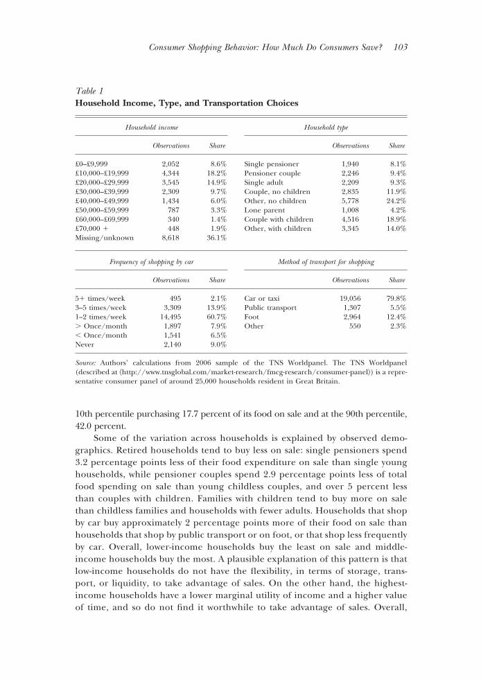
Our analysis uses data for calendar year 2006. We observe expenditure for23,877 households on purchases in 189 categories, effectively covering all food andbeverage purchases. These households made a total of 5.6 million separate shop-ping trips. On average, a single shopping trip involves the purchase of 4.2 items and£6.08 in expenditure. The average duration between shopping trips (excludingmultiple trips within the same day) is four days (with a median of three days).Table 1 provides demographic characteristics on household income, householdcomposition, how often the household shops by car, and what the most commonmode of transport is for shopping. This data is similar to that found in othernational surveys. For example, the distribution of income and the household typesin these data are similar to those found in other U.K. surveys, like the UKExpenditure and Food Survey (EFS), although overall average income is slightlylower and the market research data seem to contain somewhat fewer householdsheaded by a pensioner and fewer single adult households.2 The figures on shoppingtransport mode match very closely to Department for Transport (2005) figures.

Sales and Stockpiling

If we focus on a narrowly defined product—such as a particular brand and sizesold at a particular store—much of the price variation over time is due to temporaryprice reductions. In many cases, consumers respond to this price pattern bystockpiling for future consumption (Hendel and Nevo, 2006a; Boizot, Robin, andVisser, 2001, and references therein). When buying on sale, a consumer faces atradeoff between paying a lower price today for a product that will be consumed inthe future, and incurring a storage cost until the product is consumed. The benefitsfrom buying on sale depend on future consumption needs and on expected futureprices. Different consumers will make different choices, and a given consumer willmake different choices for different goods.

How Much Do Households Buy on Sale?The TNS data record detailed information on sales obtained from a variety of

sources, including the receipts sent in by households, fieldwork, and directly fromthe stores. Promotions typically take two forms: price promotions (half price off or£1 off, say) or quantity promotions (buy one, get one free; or double volume). Onaverage, around 29.5 percent of total annual average food expenditures are on saleitems. There is considerable variation across households, with the household at the

2 The TNS data includes demographic weights that correct for potential biases in recruiting andretaining some household types and some deliberate oversampling of others such as multiple adulthouseholds with many shoppers. We do not use these weights in this analysis, but control for observeddemographic characteristics when looking at the savings from different channels in the next sections.


10th percentile purchasing 17.7 percent of its food on sale and at the 90th percentile,42.0 percent.

Some of the variation across households is explained by observed demo-graphics. Retired households tend to buy less on sale: single pensioners spend3.2 percentage points less of their food expenditure on sale than single younghouseholds, while pensioner couples spend 2.9 percentage points less of totalfood spending on sale than young childless couples, and over 5 percent lessthan couples with children. Families with children tend to buy more on salethan childless families and households with fewer adults. Households that shopby car buy approximately 2 percentage points more of their food on sale thanhouseholds that shop by public transport or on foot, or that shop less frequentlyby car. Overall, lower-income households buy the least on sale and middle-income households buy the most. A plausible explanation of this pattern is thatlow-income households do not have the flexibility, in terms of storage, trans-port, or liquidity, to take advantage of sales. On the other hand, the highest-income households have a lower marginal utility of income and a higher valueof time, and so do not find it worthwhile to take advantage of sales. Overall,

Table 1Household Income, Type, and Transportation Choices

Household income Household type

Observations Share Observations Share

£0–£9,999 2,052 8.6% Single pensioner 1,940 8.1%£10,000–£19,999 4,344 18.2% Pensioner couple 2,246 9.4%£20,000–£29,999 3,545 14.9% Single adult 2,209 9.3%£30,000–£39,999 2,309 9.7% Couple, no children 2,835 11.9%£40,000–£49,999 1,434 6.0% Other, no children 5,778 24.2%£50,000–£59,999 787 3.3% Lone parent 1,008 4.2%£60,000–£69,999 340 1.4% Couple with children 4,516 18.9%£70,000 � 448 1.9% Other, with children 3,345 14.0%Missing/unknown 8,618 36.1%

Frequency of shopping by car Method of transport for shopping

Observations Share Observations Share

5� times/week 495 2.1% Car or taxi 19,056 79.8%3–5 times/week 3,309 13.9% Public transport 1,307 5.5%1–2 times/week 14,495 60.7% Foot 2,964 12.4%� Once/month 1,897 7.9% Other 550 2.3%� Once/month 1,541 6.5%Never 2,140 9.0%

Source: Authors’ calculations from 2006 sample of the TNS Worldpanel. The TNS Worldpanel(described at �http://www.tnsglobal.com/market-research/fmcg-research/consumer-panel�) is a repre-sentative consumer panel of around 25,000 households resident in Great Britain.

Consumer Shopping Behavior: How Much Do Consumers Save? 103

however, observed demographics explain less than 10 percent of the variationin the propensity to purchase on sale.

How Much Do Households Save by Buying On Sale?We want to compute a single saving figure for each household. Our data allows

us to identify whether or not a purchase was on sale, but not the value of the saving,and so we begin by estimating this saving. For each of our 189 food productcategories, we use a regression model whose key explanatory variable is a dummyvariable for whether the item was on sale. The model is:

ln piht � �j sit � �ij � �j � �j � eiht

where i indexes a detailed product (as defined by a unique barcode); h indexeshouseholds; t is time in weeks; j indexes food categories; p is unit price; s is a salesdummy variable equal to 1 if the product is purchased on sale; �i captures barcodespecific characteristics (allowing us to control for observed and unobserved differ-ences in product characteristics); � and � are dummies for time and region,reflecting that prices vary across time and space; and e is an idiosyncratic error. Allthe coefficients are allowed to vary by product category j.

This procedure yields 189 � coefficients which are estimates of the averagepercentage price discount obtained by purchasing items in that category on sale.Each of these coefficients is negative (sale prices are lower), all but three arestatistically significant at the 5 percent level, and all but five at the 1 percent level.The discount when buying on sale varies substantially across food categories from14 percent off at the 10th percentile to 29 percent at the 90th percentile, with amean and median of 22 percent. Some categories with especially low discounts arefruit fillings (2 percent), lard (4 percent), and sugar (10 percent), while examplesof the categories with high discounts are savoury snacks (32 percent), breakfastcereal (31 percent), and baked beans (31 percent).

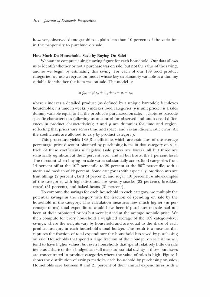
To compute the savings for each household in each category, we multiply thepotential savings in the category with the fraction of spending on sale by thehousehold in the category. This calculation measures how much higher (in per-centage terms) total expenditure would have been if purchases on sale had notbeen at their promoted prices but were instead at the average nonsale price. Wethen compute for every household a weighted average of the 189 category-levelsavings, where the weights vary by household and are equal to the share of eachproduct category in each household’s total budget. The result is a measure thatcaptures the fraction of total expenditure the household has saved by purchasingon sale. Households that spend a large fraction of their budget on sale items willtend to have higher values, but even households that spend relatively little on saleitems as a share of their budget can still make substantial savings if those purchasesare concentrated in product categories where the value of sales is high. Figure 1shows the distribution of savings made by each household by purchasing on sales.Households save between 0 and 21 percent of their annual expenditures, with a


mean of 6.5 percent. This translates into a saving of up to £794 a year, with anaverage of £96 per year.

The amount saved through buying on sale varies by observed demographics ina very similar way to the variation in the proportion of expenditure bought on sale.Most notably, poorer households and households in which the head of householdis retired save substantially less by purchasing on sale than other household types.A higher propensity to buy on sale does not necessarily mean higher savings; forexample, higher-income households purchase more on sale than lower-incomehouseholds but do not seem to realize higher savings as a result, suggesting they buyon sale in product categories in which the savings from sales are relatively low.However, as was the case with the fraction of purchases on sale, the observeddemographics explain relatively little of the variation in the savings measure.

Bulk Discounting and Choice of Package Size

Many grocery items are sold at nonlinear prices. Larger package sizes are soldat higher prices but at lower per unit price. For example, Hendel and Nevo (2006a)report that the regular, nonsale, price of a 24-pack of soft drinks cans is 2.7 timesmore than a six-pack, which implies a discount of over 30 percent in the unit price.

A consumer deciding between purchasing a smaller unit and a larger one at alower per unit price must weigh the benefits of the lower price with the costs of

Figure 1Savings Made by Households from Buying on Sale

0 5 10 15 200

500

1000

1500

2000

Household savings from sales (as a percent of annual expenditures)

Freq

uen

cy (

# of

hou

seh

olds

)

Source: Authors’ calculations from 2006 TNS sample.Notes: The histogram shows the estimated savings each household made by purchasing on sale in2006. The sample includes 23,877 households.


storing the product longer and any depreciation in the quality of the product.Different consumers will make different choices depending on their marginalutility from income, the cost of storage and transport of the product, and theirfuture consumption needs. A given consumer will make different choices fordifferent products, depending on storage costs, durability, expected consumption,and the price schedule.

How Much Do Households Buy in Bulk?Package size is reported directly in our data. To compare across a wide range

of food types, we look at how price varies across the quintiles of the package sizedistribution within each food category. The average household spends 15.8 percentof its total annual expenditure on products with the largest package sizes and 21.2,21.3, 26.8, and 14.9 percent on the other sizes from largest to smallest quintiles,respectively.

There is considerable variation across households in these fractions. For easeof exposition, we focus on the two largest quintiles as “bulk” sizes and compare thesavings made from purchasing in those two quintiles to purchases made in thesecond-largest size group (which is the most commonly purchased). Householdspurchase along the entire range of between 0 to nearly 100 percent of theirgroceries in bulk sizes, spending on average 37 percent of their budget in this sizegroup. At the 10th percentile, the figure is 24 percent, and at the 90th percentile ofhouseholds, it is 50 percent. Unsurprisingly, single-person households purchaseless in bulk than multi-person households: single nonpensioners spend around34 percent of their budget on the largest pack sizes, compared to 40 percent forcouples with children. Single pensioners make even less use of bulk discounts,spending on average 31 percent of their budget on the largest sizes. Householdsthat shop by car spend a slightly higher proportion on bulk items. The relationshipwith income is non-monotonic—the poorest households with incomes under£10,000 per year spend 36.3 percent on bulk items, those with incomes between£20,000 and £30,000 spend 37.6 percent, and those with incomes above £70,000spend 33.2 percent. Overall, the behavior of purchasing larger package sizes issimilar to purchasing on sale; in fact the two shares are positively correlated at thehousehold level, with a correlation coefficient of 0.23.

How Much Do Consumers Save By Buying In Bulk?To compute how much households save by buying in bulk, we follow a process

similar to that of sales. Our first task is to run a series of regressions, one for eachof our product categories, to estimate the magnitude of the savings made frombuying in bulk.3 We then apply these estimated savings to our actual data onhousehold purchases. The dependent variable is the log of the unit price of thegood, and the key variables are a set of dummy variables for the quintile of product

3 There are three food categories in which there is insufficient within-category product size variation tocreate size quintiles; these categories are dropped from our analysis in this part.


size in which this particular product is found (which can be interpreted relative tothe lowest quintile, which is left out). We also include our sale dummy variable fromthe earlier regression, and a set of controls for time and region. Rather thanindividual product effects, we control here for brand to capture the productcharacteristics.4 The model is:

ln piht � �jssit � �

n�2

5

�jnqi

n � �jk � �j � �j � eiht

where, qip � 1 if the pack size of product i is in the nth quintile of all products in

product group j, and zero otherwise, and where k indexes brand.Purchasing larger pack sizes results in substantial estimated savings—across all

product groups, the average unit price saving from buying in the largest sizequintile relative to the second-smallest quintile is almost 37 percent; and from thesecond-largest size quintile to the second-smallest, is 28 percent.

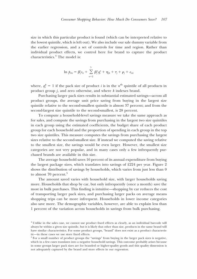
To compute a household-level savings measure we take the same approach asfor sales, and compute the savings from purchasing in the largest two size quintilesin each group using the estimated coefficients, the budget share of each productgroup for each household and the proportion of spending in each group in the toptwo size quintiles. This measure computes the savings from purchasing the largestsizes relative to the second-smallest size. If instead we computed the saving relativeto the smallest size, the savings would be even larger. However, the smallest sizecategories are not very popular, and in many cases only a few infrequently pur-chased brands are available in this size.

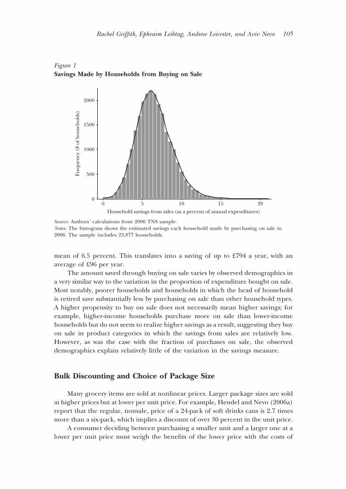
The average household saves 16 percent of its annual expenditure from buyingthe largest package sizes, which translates into savings of £224 per year. Figure 2shows the distribution of savings by households, which varies from just less than 0to almost 70 percent.5

The amount saved varies with household size, with larger households savingmore. Households that shop by car, but only infrequently (once a month) save themost in bulk purchases. This finding is intuitive—shopping by car reduces the costof transporting larger pack sizes, and purchasing larger packs on average meansshopping trips can be more infrequent. Households in lower income categoriesalso save more. The demographic variables, however, are able to explain less than1 percent of the variation across households in savings from bulk purchasing.

4 Unlike in the sales case, we cannot use product fixed effects as clearly, as an individual barcode willalways be within a given size quintile, but it is likely that other than size, products in the same brand willhave similar characteristics. For some product groups, “brand” does not exist as a product characteris-tic—in these cases we use store fixed effects.5 For a small number of product groups the “savings” from buying in the larger pack sizes is negative,which in a few cases translates into a negative household savings. This outcome probably arises becausein some groups larger pack sizes are for branded or higher-quality goods and this quality dimension isnot adequately captured by the brand and store effects in our regression.


Generic Brands and Product Choice

For many products, households have the choice of buying a generic or “store”brand. Such generic brands are typically cheaper, and some evidence shows thatconsumers substitute toward such brands as economic conditions worsen. Forexample, Gicheva, Hastings, and Villas-Boas (2007) provide evidence that consum-ers buy more store brands when gas prices rise, and Caronia (2008) finds that theincome shock caused by the Argentinean 2002 peso devaluation caused a flightfrom branded products toward store brands.

How Much Do Households Buy Store Brands?Many U.K. retailers offer own-brand products, which are targeted at different

types of consumers. The most frequently purchased are “standard” own-branditems, which are typically priced more cheaply than national brands. In addition,many retailers offer an “economy” own brand, which is cheaper still, is packagedless attractively, and is clearly aimed at very price-conscious shoppers. These econ-omy versions of store brands are probably closest to store brands in the UnitedStates. Some retailers also offer a higher-quality own-brand or “premium” productwith a focus on quality, which is priced at a similar level to national brands.

The TNS data allow us to distinguish between regular store brands andeconomy versions. Economy store brands account for on average about 3.8 percent

Figure 2Savings Made by Each Household from Buying Larger Package Sizes

0 20 40 60 80

4000

3000

2000

1000

0

Household savings from buying in bulk(as a percent of annual expenditures)

Freq

uen

cy (

# of

hou

seh

olds

)

Source: Authors’ calculations from 2006 TNS sample.Note: The histogram shows the savings each household made by purchasing larger pack sizes in 2006.The sample includes 23,877 households.


of food expenditures in 2006, while standard store brands are much more popularat 41 percent of spending. Families with children spend more on economy storebrands (5.3 of total spending for lone parents and 4.3 percent for couples withchildren), as do households on lower incomes (4.7 percent for those with incomesbelow £10,000 compared to 2.0 percent for those with incomes over £70,000).However, families with children are less likely to buy standard store brands, sug-gesting some substitutability between different forms of store own-brands.

How Much Do Households Save by Buying Store Brands?We follow the same procedure as above to measure the saving from buying

store brands; that is, we first run a regression for each separate product category toestimate how much is typically saved by purchasing store brands, and then applythese estimates to actual buying patterns. Again, log unit price is the dependentvariable; the key explanatory variables are dummy variables for products that areeconomy or standard store brands and our usual controls for time and region. Wealso include a dummy variable for the store brand defined at the level of what iscalled “fascia,” distinguishing different brands within the same chain. (For exam-ple, Tesco has three main brands—Tesco Extra, Tesco, and Tesco Metro/Express.)

Thus, the regression is:

ln piht � �jeeconi � �j

sstani � �fj � �j � �j � eiht

where f indexes fascia and econi � 1 if the product is a economy store brand andstani � 1 if the product is a standard store brand. Letting the coefficients vary bycategory allows for different quality of the store brands across categories. Onaverage, the economy store brand is almost 39 percent cheaper and the standardstore brand is 25 percent cheaper.6

As before, we compute a household-level savings measure by weighting thecategory-level savings using household-specific expenditure weights according tothe share of household spending in each category and the share of own-brandproducts in each category. Our finding is that households save on average 2 percentof their annual expenditure by buying store economy brands, with households whobuy standard store brands saving on average 3.7 percent. This translates into anaverage saving of £25 for economy own brands and £50 for standard own brands onaverage. The savings from standard store brands are larger, despite the lowerdiscounts, because the share of expenditure is much higher. There is substantialvariation across households in these savings, as for sales and bulk purchases. The10th percentile of economy savings is zero, suggesting a considerable minority ofhouseholds never purchase economy brands; for standard store brands, the10th percentile of savings is just 0.1 percent. At the 90th percentile, savings for economybrands is 4.9 percent, and for standard own brands, it is 7.6 percent. Interestingly,at least 5 percent of households realize negative “savings” from buying standard

6 We consider “premium” store brands to be comparable to branded goods, so we do not consider them.


store brands, suggesting they buy generic items that are more expensive than theirbranded alternatives. This finding illustrates that the quality distinction betweenown-brand and branded items in the U.K. can sometimes be quite small. Nohousehold realizes a negative savings from economy brands, suggesting a moreobvious quality differential between economy generic items and branded items.

Outlet Choice

Probably the largest change over the last decade in food retailing in the UnitedStates and the United Kingdom is the increased market share of a single firm:Walmart in U.S. food retailing and Tesco in U.K. food retailing. Walmart is thelargest food retailer in the United States, with sales higher than either Kroger,Supervalu-Albertsons, or Safeway, which are the largest supermarket chains. In theUnited Kingdom, Tesco has similarly gained market share rapidly. The Competi-tion Commission (2008) reports the Tesco share of grocery sales increasing from20.2 percent in 2002 to 27.6 percent in 2007. Based on slightly different data, TNS(2008) reported a Tesco grocery market share for August 2008 of 31.6 percent.However, the fraction of expenditure in Tesco varies considerably across house-holds and over products.

In our data, information on stores is collected via the households, who recordthe store of purchase for each shopping trip. For large or chain stores, the precisestore is known (that is, the address is known); for corner and local stores, thespecific store location is typically not known. Households vary substantially in theshare of their purchases made at Tesco. The average household spends 32 percentof total annual food expenditure at Tesco. However, nearly 20 percent of house-holds spend nothing at Tesco, and 1.7 percent of households spend all of their foodbudget there.7 Couples and families with children buy a larger share of theirgroceries at Tesco, as do households that shop more often by car. Higher-incomehouseholds are more likely to shop at Tesco, and lower-income households aremuch less likely to. None of these demographics explains much of the household-level variation in the share of groceries purchased at Tesco.

To discover how much households save by shopping at Tesco, we again firstestimate a series of regressions, one for each product category. The dependentvariable is the log of the unit price paid by each household for a specific good ata specific time. The key explanatory variable is a dummy variable for whether theitem was purchased at Tesco, and we also include the other control variables wehave been including throughout. Thus, the regression takes the form:

ln piht � �jTescoiht � �kj � �j � �j � eiht ,

7 As a comparison, using similar consumer-level data from the United States, we find that the averagehousehold spends 16 percent of its food expenditure at Walmart, while 23 percent of households do notpurchase any food at Walmart.


where Tescoiht � 1 if household h bought good i at time t in a Tesco store. Aspreviously, � and � are time and region dummies, and �k are brand dummies.Relative to the other dimensions, examined above, the potential savings seem muchmore modest. The average discount in Tesco is 1.6 percent, and the median is1.0 percent. There also seems to be much less heterogeneity in the savings acrossproduct categories, particularly compared to savings from generic brands and bulkdiscounting.

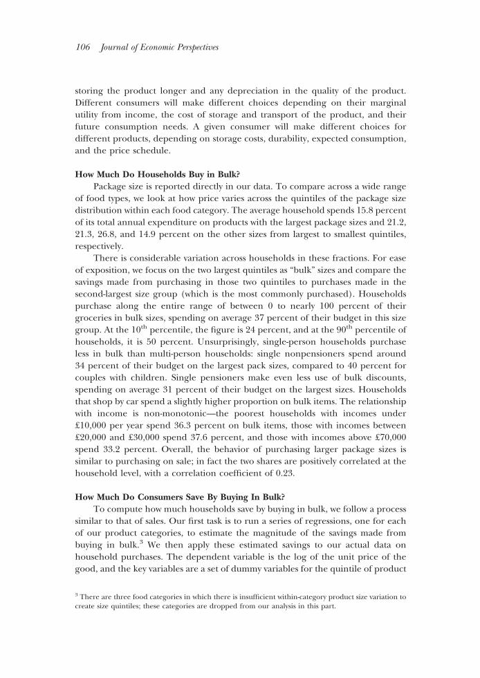
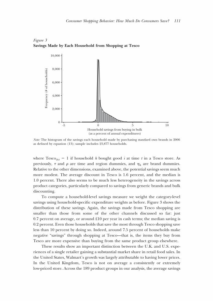
To compute a household-level savings measure we weight the category-levelsavings using household-specific expenditure weights as before. Figure 3 shows thedistribution of these savings. Again, the savings made from Tesco shopping aresmaller than those from some of the other channels discussed so far: just0.7 percent on average, or around £10 per year in cash terms; the median saving is0.2 percent. Even those households that save the most through Tesco shopping saveless than 10 percent by doing so. Indeed, around 7.5 percent of households makenegative “savings” through shopping at Tesco—that is, the items they buy fromTesco are more expensive than buying from the same product group elsewhere.

These results show an important distinction between the U.K. and U.S. expe-riences of a single retailer gaining a substantial market share in retail food sales. Inthe United States, Walmart’s growth was largely attributable to having lower prices.In the United Kingdom, Tesco is not on average a consistently or extremelylow-priced store. Across the 189 product groups in our analysis, the average savings

Figure 3Savings Made by Each Household from Shopping at Tesco

-5 0 5 10Household savings from buying in bulk(as a percent of annual expenditures)

10,000

8,000

6,000

4,000

2,000

0

Freq

uen

cy (

# of

hou

seh

olds

)

Note: The histogram of the savings each household made by purchasing standard own brands in 2006as defined by equation (13); sample includes 23,877 households.


at Tesco is 1.6 percent; nevertheless, average savings is negative (that is, Tescoprices are higher) in 79 categories.8

Pensioners and childless households save the least from Tesco shopping, whilstfamilies with children save the most. Larger savings are also made by those who shopby car, in particular those who shop once or twice a week by car. Richer households alsomake larger savings. Once again, however, these demographics are unable to explainmuch of the variation in the savings made through Tesco purchases.

Comparing the Savings

We have described four different ways in which households can seek out lowerprices when buying food: sales, bulk quantities, store brands, and outlet substitu-tions. We now assess the relative importance of these different dimensions.

We start with a comparison of potential savings that can be made (in terms oflower prices) based on the four sets of regressions described above. Recall that each setof regressions had 189 equations, one for each food category, to give estimates of thepotential savings in each food category from sales, large package sizes, generic brands,and outlet choice, controlling as far as possible for quality differences across products.Panel A of Table 2 shows the distribution of the potential savings implied by the �

coefficients in these regressions. This distribution is based entirely on differences inprices; that is, these are not weighted by the quantity of goods sold or by expenditureon different goods. The thought experiment is “how much would a household save ifit switched from buying none of its purchases on sale/in bulk/on generics/at Tesco tobuying all of its purchases on sale/in bulk/on generics/at Tesco?”

The potential savings measured in terms of price alone are highest fromeconomy generic brands, followed by bulk purchases, standard generic brands,sales, and then Tesco. Except for the savings from Tesco, these potential savingsseem to be of comparable magnitude.

Panel B of Table 2 shows the extent to which households actually make use ofthese different savings channels, summarizing the distribution of household spend-ing (as a share of total spending) on each. Expenditure shares do not track thepotential savings on each share: for example, economy generic brands offer thegreatest potential for savings, yet expenditure shares on these brands are relativelysmall. Similarly, Tesco offers small potential savings yet attracts a large share of totalspending. These findings reflect the fact that potential price savings are not theonly motivation for shopping choices—economy generics may well be lower qualitythan standard generics or branded items and are not always available in all storetypes; Tesco stores may compete on nonprice grounds or may simply be more orless conveniently located for different households.

8 In fact, the U.K. retailer that is closest to Walmart is Asda—which was taken over by Walmart in 1999.Asda advertises itself as a low-priced store. However, it has not experienced the same growth in marketshare as Walmart has in the United States.


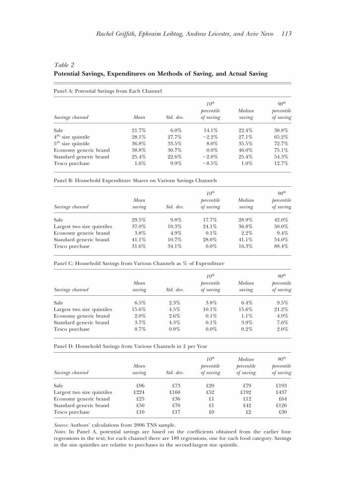
Table 2Potential Savings, Expenditures on Methods of Saving, and Actual Saving

Panel A: Potential Savings from Each Channel

Savings channel Mean Std. dev.

10th

percentileof saving

Mediansaving

90th

percentileof saving

Sale 21.7% 6.0% 14.1% 22.4% 38.8%4th size quintile 28.1% 27.7% �2.2% 27.1% 65.2%5th size quintile 36.8% 33.5% 8.0% 35.5% 72.7%Economy generic brand 38.8% 30.7% 0.0% 46.0% 75.1%Standard generic brand 25.4% 22.6% �2.0% 25.4% 54.3%Tesco purchase 1.6% 9.9% �8.5% 1.0% 12.7%

Panel B: Household Expenditure Shares on Various Savings Channels

Savings channelMeansaving Std. dev.

10th

percentileof saving

Mediansaving

90th

percentileof saving

Sale 29.5% 9.8% 17.7% 28.9% 42.0%Largest two size quintiles 37.0% 10.3% 24.1% 36.8% 50.0%Economy generic brand 3.8% 4.9% 0.1% 2.2% 9.4%Standard generic brand 41.1% 10.7% 28.0% 41.1% 54.0%Tesco purchase 31.6% 34.1% 0.0% 16.3% 88.4%

Panel C: Household Savings from Various Channels as % of Expenditure


10th

percentileof saving

Mediansaving

90th

percentileof saving

Sale 6.5% 2.3% 3.8% 6.4% 9.5%Largest two size quintiles 15.6% 4.5% 10.1% 15.6% 21.2%Economy generic brand 2.0% 2.6% 0.1% 1.1% 4.9%Standard generic brand 3.7% 4.3% 0.1% 3.9% 7.6%Tesco purchase 0.7% 0.9% 0.0% 0.2% 2.0%

Panel D: Household Savings from Various Channels in £ per Year


10th

percentileof saving

Medianpercentileof saving

90th

percentileof saving

Sale £96 £73 £20 £79 £193Largest two size quintiles £224 £160 £52 £192 £437Economy generic brand £25 £36 £1 £12 £64Standard generic brand £50 £70 £1 £42 £126Tesco purchase £10 £17 £0 £2 £30

Source: Authors’ calculations from 2006 TNS sample.Notes: In Panel A, potential savings are based on the coefficients obtained from the earlier fourregressions in the text; for each channel there are 189 regressions, one for each food category. Savingsin the size quintiles are relative to purchases in the second-largest size quintile.


Looking more closely at this data, households who buy more on sale alsopurchase in bulk, which is reasonable since both these choices are driven by storagecosts. On the other hand, households that buy on sale tend to spend less on genericgoods (a similar finding for U.S. data is in Leibtag and Kaufman, 2003). Similarly,households that buy economy generic also tend to purchase in bulk.

Panels C and D of Table 2 combine the potential savings in Panel A with thehousehold expenditure choices in Panel B to estimate the actual savings thathouseholds obtain from these different choices. In Panel C, we express this savingsin terms of percentage of expenditure, while in Panel D, we present the savings inBritish pounds per year. The savings from bulk purchasing are the largest, followedby savings from sales, purchases of generics (standard then economy), and shop-ping at Tesco. The relatively large savings from bulk purchases reflect both theirlarge potential saving (Panel A) and their high expenditure share (Panel B). Forstandard generic brands, both the potential savings and expenditure shares wererelatively high but the actual savings are quite low. This outcome occurs becausethe item categories where the generic expenditure share is higher are also thosewhere the potential savings are relatively low (which may imply that the differencebetween generic brands and branded products is also quite low, meaning house-holds are more willing to substitute toward generic brands).

Some warnings should be issued about interpreting these estimates. First, theydo not account for the costs of savings. In the case of sales and bulk purchases, thesecosts involve storage and transport, and potential depreciation in the quality of theproduct over time. For generic brands, the cost could include quality differences.For outlet choice, travel costs as well as potential quality differences between storescould be important. These savings could therefore be interpreted as “gross” savings,but the “net” savings from the different channels may not be of the same magnitudeor even rank. An additional warning is that the savings measures overlap. Forexample, if products sold in Tesco are more frequently on sale, the correspondingsavings are potentially counted twice, both in Tesco and in the sales measures; onecould think of estimating these savings jointly in a single model, but it is thenharder to interpret the individual effects.

The savings vary with household demographics. Retired households tend to beless likely to save on any of the four dimensions relative to other household groups.Childless couples and single adults are next, with an intermediate willingness totake advantage of these methods of saving. Families with children tend to save morethrough each of the savings channels than those without children, with the highestrelative gains for bulk discounting and sales. This pattern makes sense: largerfamilies have larger consumption needs and so they are more likely to benefit fromsales and bulk purchasing for a given storage cost.

Figure 4 shows the estimated savings from each channel according to house-hold income relative to households with low incomes below £10,000 per year. Bulkpurchases and economy brands follow the same pattern, with savings decreasingmonotonically with income, showing that these channels are used most by low-income households. By contrast, saving from sales (and, to a lesser extent, from


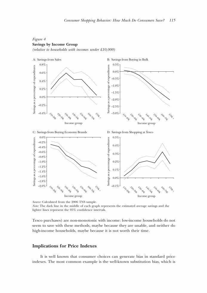
Tesco purchases) are non-monotonic with income: low-income households do notseem to save with these methods, maybe because they are unable, and neither dohigh-income households, maybe because it is not worth their time.

Implications for Price Indexes

It is well known that consumer choices can generate bias in standard priceindexes. The most common example is the well-known substitution bias, which is

Figure 4Savings by Income Group(relative to households with incomes under £10,000)

0.8%

0.6%

0.4%

0.2%

0.0%

–0.2%

–0.4%

0.5%

0.0%

–0.5%

–1.0%

–1.5%

–2.0%

–2.5%

–3.0%

0.0%

–0.2%

–0.4%

–0.6%

–0.8%

–1.0%

–1.2%

–1.4%

–1.6%

–1.8%

–2.0%

0.5%

0.4%

0.3%

0.2%

0.1%

0.0%

–0.1%

A: Savings from Sales B: Savings from Buying in Bulk

C: Savings from Buying Economy Brands D: Savings from Shopping at Tesco

Savi

ngs a

s a p

erce

ntag

e of

exp

endi

ture

sSa

ving

s as a

per

cent

age

of e

xpen

ditu

res

Savi

ngs a

s a p

erce

ntag

e of

exp

endi

ture

sSa

ving

s as a

per

cent

age

of e

xpen

ditu

res

Income group Income group

Income groupIncome group

£10–20k

£20–30k

£30–40k

£40–50k

£50–60k

£60–70k

£70k +£10–20k

£20–30k

£30–40k

£40–50k

£50–60k

£60–70k

£70k +

£10–20k

£20–30k

£30–40k

£40–50k

£50–60k

£60–70k

£70k +

£10–20k

£20–30k

£30–40k

£40–50k

£50–60k

£60–70k

£70k +

Source: Calculated from the 2006 TNS sample.Note: The dark line in the middle of each graph represents the estimated average savings and thelighter lines represent the 95% confidence intervals.


easiest to illustrate in its pure form. Suppose a consumer consumes two products,rice and potatoes. Initially both products cost $1 per pound, and the consumerchooses one pound of each. In the second period, the price of rice increases to $2,but the price of potatoes is unchanged. Using a fixed bundle consisting of onepound of each product, the measured increase in the price index is 50 percent. Ifrice and potatoes are perfect substitutes, then the consumer will simply substitutepotatoes instead of the rice with no loss of utility, and so the price index willconsiderably overstate the true change in the cost of living. However, assume thatthe two goods are not perfect substitutes, and as relative prices change, theconsumer substitutes from rice to potatoes and consumes, for example, 1.5 poundsof potatoes and only 0.5 pounds of rice. The actual increase in expenditure is nowonly 25 percent, which is also the measured price increase using the second-periodbundle—measured this way, the possibility for substitution would overestimate theprice increase. However, it should be remembered that the consumer has lost utilitybeing pushed to substitute from rice to potatoes, and the measured change inexpenditure does not take this utility loss into account, so the 25 percent increasein expenditure underestimates the loss in utility that has occurred.

Similar logic suggests that a price index based on a fixed basket of goods willmiss a shift toward the cheaper own brand, especially if store branded products areunder-sampled in the bundle used to compute the price index. (We do not knowwhether branded products are over- or under-sampled in the U.K. food price index;our point here is a general methodological one that if they are, then this sort of biaswill result.)

For the purposes of constructing price indexes, the implications of “outletsubstitution”—that is, the effect of consumers shifting their purchases to differentand less-expensive retail outlets—have been well documented (for example,Reinsdorf, 1994; Boskin, Dulberger, Gordon, Grilliches, and Jorgenson, 1998;Hausman and Leibtag, 2004). In the United States, the way that prices havetraditionally been collected may not fully capture price changes in retailers likeWalmart, or the approach treats the price difference between Walmart and othersas a reflection of quality, rather than a genuine lower price. The situation issomewhat different in the United Kingdom; the national statistical agency, theOffice for National Statistics, does attempt to reflect the annual changes in super-market share when calculating food and grocery price indices.

Consumer stockpiling in reaction to sales also has implications for the stan-dard measurement of price indices. It implies a separation between a standardprice index based on purchase prices and a consumption-based price index thatshould account for the ability to store the product. To illustrate the difference,consider the following example: Suppose a consumer consumes two products, Aand B, at equal quantities. Product A always costs $2, while product B is normallypriced at $2, but goes on sale for one period and is sold at a price of $1. Normally,the consumer purchases one unit of each product each period and consumes bothproducts in that period. Suppose the consumer has a storage cost of $0.25 per unitper period. When product B goes on sale, the consumer purchases four units and


consumes one unit each week over the next few weeks. We assume the consumerdoes not increase consumption in response to the sale price; we also ignore theconsumer’s discount factor. The consumer saves on each of the units that ispurchased and stored; for the last unit, for example, the consumer pays $1 andstores it for three periods at a total cost of $0.75, for a total saving of $0.25 relativeto buying the product at the regular $2 price. The consumer, however, will not savefrom buying additional units above the four purchased because of the storage costs.If the consumer bought a fifth unit on sale, the storage costs for the unit for fourperiods will exactly equal the savings (and so we assume that in this case theconsumer will not store the product).

Suppose we want to compute a cost-of-living index for this consumer. We setthe base as the price during nonsale periods, so when consuming one unit of eachproduct, the base is $4. The consumption-based price index for the period of thesale and the following weeks is (2.00 � 1.00)/4.00 � 0.75 for the sale period;(2.00 � 1.25)/4.00 � 0.8125 for the next week; (2.00�1.50)/4.00 � 0.875 for thenext week; (2.00�1.75)/4.00 � 0.9375 for the next week; and then 1.00 for everyfollowing week when the sale has ended and no further consumption of storedproducts occurs. A standard price index will capture some price reduction in theweek of the sale, depending on the quantity weight used to compute the index.However, a standard price index will not capture the effective drop in the priceindex in the weeks following the sale—and the problem cannot be “fixed” byadjusting the weights. Aggregation across weeks to construct a monthly price willalso not solve the problem even if the timing is captured properly. In this case, theaggregation will overestimate the benefits from purchasing on sale because it willignore the storage cost.

The issues in measurement of a price index with bulk goods and varying unitprices are very similar to those that arise in the case of sales. First, there is an issueof whether statistical agencies correctly sample all the relevant prices. In the UnitedKingdom, the specification of food items to be collected as part of the basket ofitems used to calculate inflation rates typically contains an exact size that must bepriced. It is unusual for different sizes of the same product to be sampled and thereis no way to account for a change in the relative price of different sizes. As priceschange, the tradeoffs between different sizes, and therefore consumer choices, willchange. Without sampling different sizes of goods, statistical agencies will miss thiseffect and compute an index that overestimates price increases.

Occasionally, statistical agencies will sample different package sizes (whenproducts change, for example, and firms replace a pack of one size with anothersize). A common response by statistical agencies is to link the price from differentsizes using unit values. For example, if a pack of 100g priced normally at £1 is notavailable, but instead the item is only available as a 200g pack priced at £1.80, theagency will “pretend” the price is £0.90 per 100g. However, this practice is onlyjustified if prices are linear in package size, which is rarely the case. Otherwise, aspointed out by Triplett (2004), this approach will underestimate the price index.

The savings measures we presented above do not allow us to quantify directly


the effect of the various choices made by consumers on the measurement of theprice index. To measure these effects we need to compute a standard price index,which ignores the substitution effects, and compare it to a price index that accountsfor the different forms of substitution. Previous work has estimated the effect ofsubstitution bias as well as outlet bias, and has found it to be significant. Our resultssuggest that the bias due to stockpiling and bulk purchases have the potential to beof the same order of magnitude.

Concluding Comments

In this paper, we have documented the potential and actual savings thatconsumers in the U.K. realize from various forms of substitution. The resultssuggest that savings from sales and bulk buying are of a similar order of magnitudeto those due to economy brands and outlet choice. The data in this paper comefrom the United Kingdom; an interesting question is how these findings arecomparable to other countries. Preliminary analysis of similar data from the UnitedStates suggests similar findings, although with some interesting differences. Salesand bulk purchases, and the savings they entail, seem to be even more significantin the United States. This pattern should not be surprising. On average, U.S. homesare larger and consumers tend to shop more with cars, so transport and storagecosts are lower. As a result, larger sizes not only tend to be more often purchasedin the United States but also offered more by stores; for example, a gallon-sizeice-cream pack is quite popular in the United States but is typically not available inthe United Kingdom. Store brands are also different in the United States andtypically less important than in the United Kingdom. As discussed earlier, thesavings from Walmart seem to be more significant than the savings from shoppingat Tesco. Taking these factors together, our conclusion that savings from sales andbulk purchases are important probably holds with even greater force in the U.S.economy. Further cross-national comparisons of how these savings vary acrosshouseholds would be interesting; Aguiar and Hurst (2007), for example, usedscanner data similar to the data used in this study, and found that poorer and olderhouseholds typically paid lower prices for identical products than younger, richerhouseholds and that families with children paid the highest prices. Given that sales,bulk purchasing, store choice, and branding all influence the price paid foressentially identical items, these channels of saving will be crucial in determiningwho pays more and whether the pattern of relative prices differs across countries.

Data on household consumption that include barcodes for specific products,details about stores, and a range of household information are a relatively recentdevelopment for academic economists. Economists are still learning how to exploreand exploit their possibilities. Future research may, for example, take the costs oftransportation and storage into account, and eventually be able to estimate a fulldemand system incorporating these different elements of purchasing behaviors.Other research will doubtless look at these data from the perspective of nutritional


choices, or from the perspective of how much flexibility households have to adjusttheir costs by changing their shopping or purchasing behavior.

This work also has implications for improving the consumer price index. Astandard price index based on a fixed basket of goods will overstate the rise in thetrue cost of living because it does not properly consider sales and bulk purchasing.According to our measures, the extent of this bias might be of the same or evengreater magnitude than the better-known substitution and outlet biases. Yet biasesdue to sales and bulk purchasing have received much less attention in the priceindex literature. We second Triplett (2003) in suggesting that this is a fruitful areafor future research.

y Financial support for Griffith and Leicester from the ESRC through the ESRC Centre for theMicroeconomic Analysis of Public Policy at IFS (CPP) is gratefully acknowledged. We wish tothank the editors of this journal and seminar participants at the U.S. Bureau of EconomicAnalysis and the 2008 World Congress on National Accounts and Economic PerformanceMeasures for Nations for their comments and suggestions. The views expressed herein are thoseof the authors and do not necessarily reflect the views of the U.S. Department of Agriculture.

References

Aguiar, Mark, and Erik Hurst. 2007. “Life-Cycle Prices and Production.” American EconomicReview, 97(5): 1533–59.

Baye, Michael R. 1985. “Price Dispersion andFunctional Price Indices.” Econometrica, 53(1):213–23.

Boizot, Christine, Jean-Marc Robin, and Mi-chael Visser. 2001. “The Demand for Food Prod-ucts: An Analysis of Interpurchase Times andPurchased Quantities.” The Economic Journal,111(470): 391–419.

Boskin, Michael J., Ellen R. Dulberger, RobertJ. Gordon, Zvi Griliches, and Dale W. Jorgenson.1998. “Consumer Prices, the Consumer PriceIndex, and the Cost of Living.” Journal of Eco-nomic Perspectives, 12(1): 3–26.

Caronia, Mateo. 2008. “The Microeconomicsof Large Devaluations.” Unpublished paper,Northwestern University.

Competition Commission. 2008. Appendix3.1 of “Market Investigation into the Supply ofGroceries in the UK.” http://www.competition-commission.org.uk/rep_pub/reports/2008/fulltext/538_3_1.pdf.

Crawford, Ian. 1996. “UK Household Cost-of-Living Indices, 1979–92.” In New Inequalities: TheChanging Distribution of Income and Wealth in theUnited Kingdom, ed. John Hills, chap. 4. Cam-bridge University Press.

Crawford, Ian, and Zoe Smith. 2002. “Distri-butional Aspects of Inflation.” IFS Commentary90. London: Institute for Fiscal Studies. http://www.ifs.org.uk/comms/comm90.pdf.

Deaton, Angus. 1998. “Getting Price Right:What Should Be Done?” The Journal of EconomicPerspectives, 12(1): 37–46.

Deaton, Angus, and John Muellbauer. 1980.Economics and Consumer Behavior. CambridgeUniversity Press.

Department for Transport. 2005. Focus on Per-sonal Travel 2005 Edition. London: The StationeryOffice. http://www.dft.gov.uk/pgr/statistics/datatablespublications/personal/focuspt/2005/focusonpersonaltravel2005edi5238

Diewert, W. E. 1993. “The Early History ofPrice Index Research.” In Essays in Index Num-ber Theory, Volume 1, Contributions to Eco-nomic Analysis 217, ed. W. E. Diewert and


A. O. Nakamura, 33– 65. Amsterdam: NorthHolland.

Feenstra, Robert C., and Matthew D. Shapiro.2003. “High-Frequency Substitution and theMeasurement of Price Indexes.” In Scanner Dataand Price Indexes, 123–150. University of ChicagoPress.

Gicheva, Dora, Justine Hastings, and Sofia B.Villas-Boas. 2007. “Revisiting the Income Effect:Gasoline Prices and Grocery Purchases.” NBERWorking Paper 13614.

Hausman, Jerry. 2003. “Sources of Bias andSolutions to Bias in the Consumer Price Index.”The Journal of Economic Perspectives, 17(1): 23–44.

Hausman, Jerry, and Ephraim Leibtag. 2004.“CPI Bias from Supercenters: Does the BLSKnow That Wal-Mart Exists?” NBER WorkingPaper 10712.

Hausman, Jerry, and Ephriam Leibtag. 2007.“Consumer Benefits from Increased Competi-tion in Shopping Outlets: Measuring the Effectof Wal-Mart.” Journal of Applied Econometrics,22(7): 1157–77.

Hendel, Igal, and Aviv Nevo. 2006a. “Salesand Consumer Inventory.” The RAND Journal ofEconomics, 37(3): 543–61.

Hendel, Igal, and Aviv Nevo. 2006b. “Measur-ing the Implications of Sales and Consumer In-ventory Behavior.” Econometrica, 74(6): 1637–73.

Leibtag, Ephram, and Phil R. Kaufman. 2003.“Exploring Food Purchase Behavior of Low-In-come Households: How Do They Economize?”Agriculture Information Bulletin No. 747-07.http://www.ers.usda.gov/Publications/AIB747/aib74707.pdf.

Leicester, Andrew, Cormac O’Dea, and ZoeOldfield. 2008. “The Inflation Experience ofOlder Households.” IFS Commentary 106. Lon-don: Institute for Fiscal Studies. http://www.ifs.org.uk/comms/comm106.pdf.

Office for National Statistics. 2007. “ConsumerPrices Index Technical Manual.” http://www.statistics.gov.uk/downloads/theme_economy/CPI_Technical_Manual.pdf.

Pollak, Robert A. 1998. “The Consumer PriceIndex: A Research Agenda and Three Propos-als.” The Journal of Economic Perspectives, 12(1):69–78.

Reinsdorf, Marshall. 1994. “The Effect ofPrice Dispersion on Cost of Living Indexes.”International Economic Review, 35(1): 137–49.

Schultze, Charles L. 2003. “The ConsumerPrice Index: Conceptual Issues and PracticalSuggestions.” Journal of Economic Perspectives,17(1): 3–22.

TNS. 2008. “Price Now Clearly Driving MarketShares.” Press Release, August, 19. http://www.tnsglobal.com/_assets/files/TNS_Market_Research_Supermarket_Share_data_mmentary.pdf.

Triplett, Jack E. 2003. “Using Scanner Data inConsumer Price Indexes: Some Neglected Con-ceptual Considerations.” In Scanner Data andPrice Indexes, ed R. C. Feenstra and M. D. Sha-piro, p 151–162. University of Chicago Press.

Triplett, Jack E. 2004. “Handbook on Hedo-nic Indexes and Quality Adjustments in PriceIndexes: Special Application to InformationTechnology Products.” OECD Science, Technol-ogy and Industry Working Papers, 2004/9.


This article has been cited by:

1. Yu Ma, Kusum L Ailawadi, Dinesh K Gauri, Dhruv Grewal. 2011. An Empirical Investigation of theImpact of Gasoline Prices on Grocery Shopping Behavior. Journal of Marketing 75:2, 18-35. [CrossRef]

2. J. L. Lusk, K. Brooks. 2011. Who Participates in Household Scanning Panels?. American Journal ofAgricultural Economics 93:1, 226-240. [CrossRef]

3. John S. Greenlees, Robert McClelland. 2010. New Evidence on Outlet Substitution Effects in ConsumerPrice Index Data. Review of Economics and Statistics 110301164542093. [CrossRef]

4. Andrew Leicester, ZoÃ« Oldfield. 2009. Using Scanner Technology to Collect Expenditure Data*. FiscalStudies 30:3-4, 309-337. [CrossRef]

5. Rachel Griffith, Martin O'Connell. 2009. The Use of Scanner Data for Research into Nutrition*. FiscalStudies 30:3-4, 339-365. [CrossRef]

http://dx.doi.org/10.1509/jmkg.75.2.18

http://dx.doi.org/10.1093/ajae/aaq123

http://dx.doi.org/10.1162/REST_a_00107

http://dx.doi.org/10.1111/j.1475-5890.2009.00098.x

http://dx.doi.org/10.1111/j.1475-5890.2009.00099.x

consumer shopping behavior: how much do...

Documents