constructions and classifications of projective poisson ... · pdf fileconstructions and...

Lett Math Phys (2018) 108:573–632https://doi.org/10.1007/s11005-017-0984-5

Constructions and classifications of projective Poissonvarieties

Brent Pym1

Received: 30 January 2017 / Revised: 5 August 2017 / Accepted: 11 August 2017 /Published online: 13 September 2017© The Author(s) 2017. This article is an open access publication

Abstract This paper is intended both as an introduction to the algebraic geometryof holomorphic Poisson brackets, and as a survey of results on the classification ofprojective Poisson manifolds that have been obtained in the past 20years. It is basedon the lecture series delivered by the author at the Poisson 2016 Summer Schoolin Geneva. The paper begins with a detailed treatment of Poisson surfaces, includingadjunction, ruled surfaces and blowups, and leading to a statement of the full birationalclassification. We then describe several constructions of Poisson threefolds, outliningthe classification in the regular case, and the case of rank-one Fano threefolds (such asprojective space). Following a brief introduction to the notion of Poisson subspaces,we discuss Bondal’s conjecture on the dimensions of degeneracy loci on Poisson Fanomanifolds.We close with a discussion of log symplectic manifolds with simple normalcrossings degeneracy divisor, including a new proof of the classification in the case ofrank-one Fano manifolds.

Keywords Poisson bracket · Fano manifold · Singularity theory · Degeneracy loci

Mathematics Subject Classification 14J45 · 14N05 · 17B63 · 53D17

Contents

1 Introduction . . . . . . . . . . . . . . . . . . . . . . . . . . . . . . . . . . . . . . . . . . . . . 5741.1 Basic definitions and aims . . . . . . . . . . . . . . . . . . . . . . . . . . . . . . . . . . . . 5741.2 What is meant by classification? . . . . . . . . . . . . . . . . . . . . . . . . . . . . . . . . 577

B Brent [email protected]

1 School of Mathematics, University of Edinburgh, James Clerk Maxwell Building,The King’s Buildings, Peter Guthrie Tait Road, Edinburgh EH9 3FD, UK

123

http://crossmark.crossref.org/dialog/?doi=10.1007/s11005-017-0984-5&domain=pdf

574 B. Pym

1.3 The role of Fano manifolds . . . . . . . . . . . . . . . . . . . . . . . . . . . . . . . . . . . 5782 Poisson surfaces . . . . . . . . . . . . . . . . . . . . . . . . . . . . . . . . . . . . . . . . . . . 579

2.1 Basics of Poisson surfaces . . . . . . . . . . . . . . . . . . . . . . . . . . . . . . . . . . . 5792.2 Poisson structures on the projective plane . . . . . . . . . . . . . . . . . . . . . . . . . . . 5822.3 Anticanonical divisors and adjunction . . . . . . . . . . . . . . . . . . . . . . . . . . . . . 5842.4 Poisson structures on ruled surfaces . . . . . . . . . . . . . . . . . . . . . . . . . . . . . . 5872.5 Blowups and minimal surfaces . . . . . . . . . . . . . . . . . . . . . . . . . . . . . . . . . 5932.6 Birational classification of Poisson surfaces . . . . . . . . . . . . . . . . . . . . . . . . . . 598

3 Poisson threefolds . . . . . . . . . . . . . . . . . . . . . . . . . . . . . . . . . . . . . . . . . . 6023.1 Regular Poisson structures . . . . . . . . . . . . . . . . . . . . . . . . . . . . . . . . . . . 6023.2 Poisson structures from pencils of surfaces . . . . . . . . . . . . . . . . . . . . . . . . . . . 6043.3 Further constructions . . . . . . . . . . . . . . . . . . . . . . . . . . . . . . . . . . . . . . 6103.4 Poisson structures on P

3 and other Fano threefolds . . . . . . . . . . . . . . . . . . . . . . 6124 Poisson subspaces and degeneracy loci . . . . . . . . . . . . . . . . . . . . . . . . . . . . . . . 613

4.1 Poisson subspaces and multiderivations . . . . . . . . . . . . . . . . . . . . . . . . . . . . 6134.2 Vector fields and multiderivations . . . . . . . . . . . . . . . . . . . . . . . . . . . . . . . . 6144.3 Degeneracy loci . . . . . . . . . . . . . . . . . . . . . . . . . . . . . . . . . . . . . . . . . 615

5 Log symplectic structures . . . . . . . . . . . . . . . . . . . . . . . . . . . . . . . . . . . . . . 6195.1 Definition and examples . . . . . . . . . . . . . . . . . . . . . . . . . . . . . . . . . . . . . 6195.2 Some classification results . . . . . . . . . . . . . . . . . . . . . . . . . . . . . . . . . . . 6225.3 The simple normal crossings case . . . . . . . . . . . . . . . . . . . . . . . . . . . . . . . . 624

References . . . . . . . . . . . . . . . . . . . . . . . . . . . . . . . . . . . . . . . . . . . . . . . . 630

1 Introduction

1.1 Basic definitions and aims

This paper is an introduction to the geometry of holomorphic Poisson structures,i.e. Poisson brackets on the ring of holomorphic or algebraic functions on a com-plex manifold or algebraic variety (and sometimes on more singular objects, such asschemes and analytic spaces). It grew out of a mini-course delivered by the author atthe “Poisson 2016” summer school in Geneva. The theme for the course was how themethods of algebraic geometry can be used to construct and classify Poisson brack-ets. Hence, this paper also serves a second purpose: it is an overview of results onthe classification of projective Poisson manifolds that have been obtained by severalauthors over the past couple of decades, with some added context for the results andthe occasional new proof.

When one first encounters Poisson brackets, it is often in the setting of classicalmechanics, which is usually formulated using C∞ manifolds. However, there aremany situations in which one naturally encounters Poisson brackets that are actuallyholomorphic:

• Classical integrable systems• Moduli spaces in gauge theory, algebraic geometry and low-dimensional topology• Noncommutative ring theory• Lie theory and geometric representation theory• Cluster algebras• Generalized complex geometry• String theory• …

123

Constructions and classifications of projective Poisson 575

One is therefore lead to develop the holomorphic theory in parallel with its C∞ coun-terpart. While the two settings have much in common, there are also many importantdifferences. These differences are a consequence of the rigidity of holomorphic andalgebraic functions, and they will play a central role in our discussion.

The first (albeit minor) difference comes already in the definition: while a Poissonbracket on a C∞ manifold is simply defined by a Poisson bracket on the ring of globalsmooth functions, this definition is no longer appropriate in the holomorphic setting.The problem is that a complex manifold X may have very few global holomorphicfunctions; for instance, if X is compact and connected, then the maximum principleimplies that every holomorphic function on X is constant. Thus, in order to definethe bracket on X, we must define it in local patches which can be glued together in aglobally consistent way. In other words, we should replace the ring of global functionswith the corresponding sheaf:

Definition 1.1 Let X be a complex manifold or algebraic variety, and denote by OXits sheaf of holomorphic functions. A (holomorphic) Poisson structure on X is aC-bilinear operation

{·, ·} : OX × OX → OX

satisfying the usual axioms for a Poisson bracket. Namely, for all f, g, h ∈ OX, wehave the following identities

1. Skew-symmetry:

{ f, g} = −{g, f }

2. Leibniz rule:

{ f, gh} = { f, g}h + g{ f, h}

3. Jacobi identity:

{ f, {g, h}} + {g, {h, f }} + {h, { f, g}} = 0.

Let us denote by TX the sheaf of holomorphic vector fields on X. These are holo-morphic sections of the tangent bundle of X, or equivalently, they are derivations ofOX. As in the C∞ setting, a holomorphic Poisson bracket can be encoded in a globalholomorphic bivector field

π ∈ �(X,∧2TX),

using the pairing between vectors and forms: { f, g} = 〈d f ∧ dg, π〉. Thus, in localholomorphic coordinates x1, . . . , xn , we have

π =∑

i< j

π i j∂xi ∧ ∂x j

123

576 B. Pym

where π i j = {xi , x j } denotes the Poisson brackets of the coordinates. The Jacobiidentity for the bracket is equivalent to the condition

[π, π ] = 0 ∈ �(X,∧3TX).

on the Schouten bracket of π .Every function f ∈ OX has a Hamiltonian vector field

H f = ιd f π ∈ TX

which acts as a derivation on g ∈ OX by

H f (g) = { f, g}.

If we start at a point p ∈ X and apply the flows of all possible Hamiltonian vectorfields, we sweep out an even-dimensional immersed complex submanifold, calledthe leaf through p. The bivector can then be restricted to the leaf, and inverted toobtain a holomorphic symplectic form. Thus,X has a natural foliation by holomorphicsymplectic leaves. This foliation will typically be singular, in the sense that there willbe leaves of many different dimensions.

One of the major challenges in Poisson geometry is to deal in an efficient mannerwith the singularities of the foliation, and this is an instance where the holomorphicsetting departs significantly from the C∞ one. Indeed, the powerful tools of algebraicgeometry givemuch tighter control over the local and global behaviour of holomorphicPoisson structures.

Thus, our aim is to give some introduction to how an algebraic geometer mightthink about Poisson brackets. We will focus on the related problems of constructionand classification: how do we produce holomorphic Poisson structures on compactcomplex manifolds, and how do we know when we have found them all?

The paper is organized as a sort of induction on dimension. We begin in Sect. 2with a detailed discussion of Poisson surfaces, focusing in particular on the projectiveplane, ruled surfaces and blowups, and culminating in a statement of the full bira-tional classification [6,38]. In Sect. 3, we discuss many types of Poisson structures onthreefolds—enough to cover all of the cases that appear in the classifications of regularPoisson threefolds [21], and Poisson Fano threefolds with cyclic Picard group [13,48].Section 4 discusses the general notions of Poisson subspaces and degeneracy loci(where the foliation has singularities). We highlight the intriguing phenomenon ofexcess dimension that is commonplace for these loci, as formulated in a conjecture ofBondal.

We close in Sect. 5 with an introduction to log symplectic manifolds: Poissonmanifolds that have an open dense symplectic leaf, but degenerate along a reducedhypersurface. We give many natural examples and discuss in some detail the case inwhich the hypersurface is a simple normal crossings divisor, leading to a streamlinedproof of the classification [47] for Fano manifolds with cyclic Picard group. We alsomention a recent result of the author [56] in the case of elliptic singularities. Although

123


the material in this section was not covered in the lecture series, the author felt that itshould be included here, given the focus on classification.

The lecture series on which this article is based was intended for an audiencethat already has some familiarity with Poisson geometry, but has potentially had lessexposure to algebraic or complex geometry.We have tried to keep this article similarlyaccessible. Thus, we recall a number of basic algebro-geometric concepts (at the levelof Griffiths andHarris’ book [30]) by illustrating how they arise in our specific context.On the other hand, we hope that because of the focus on examples, experts in algebraicgeometry will also find this article useful, both as an introduction to the geometry ofPoisson brackets, and as a guide to the growing literature on the subject. Either way,the reader may find it helpful to complement the present article with a more theoreticaltreatment of the foundations, such as Polishchuk’s paper [53], the books by Dufour–Zung [23], Laurent-Gengoux–Pichereau–Vanhaecke [46], and Vanhaecke [68] and theauthor’s PhD thesis [54].

1.2 What is meant by classification?

Before we begin, we should make a few remarks to clarify what we mean by “classifi-cation” of Poisson structures. There are essentially two types of classifications: localand global.

In the local case, one is looking for nice local normal forms for Poisson brackets—essentially, coordinate systems inwhich the Poisson bracket takes on a simple standardform. While these issues will come up from time to time, they will not be the mainfocus of this paper.We instead encourage the interested reader to consult the book [23]for an introduction.

In the global case, one would ideally like a list of all compact holomorphic Poissonmanifolds (up to isomorphism), but there are far too many such manifolds to have anyreasonable hope of classification. One way to get some control over the situation isto look for a birational classification, i.e. a list of Poisson manifolds from which allothers can be constructed by simple transformations, such as blowing up. As we shallsee, this program has been completely realized in the case of surfaces.

Another way to get some control is to focus our attention on classifying all Poissonstructures on a fixed compact complex manifold X. To see that this is potentiallya tractable problem, we observe that the space �(X,∧2TX) of bivector fields isa finite-dimensional complex vector space. When written in a basis for this vec-tor space, the integrability condition [π, π ] = 0 amounts to a finite collection ofhomogeneous quadratic equations. These equations therefore determine an algebraicsubvariety

Pois(X) ⊂ �(X,∧2TX),

so that we can try to understand the moduli space of Poisson structures on X, i.e. thequotient

123

578 B. Pym

Pois(X)

Aut(X),

where Aut(X) is the group of holomorphic automorphisms of X.In general, the moduli space will have many (but only finitely many) irreducible

components, corresponding to qualitatively different types of Poisson structures onX. A reasonable goal for the classification is to list all of the irreducible componentsof the moduli space and describe the geometry of the Poisson structures that corre-spond to some dense open subset in each component. Achieving this goal gives one afairly good understanding of the qualitative behaviour of Poisson structures on X. Aswe shall see, this programme has now been carried out for several important three-dimensional manifolds, particularly the projective spaceP

3. But in higher dimensions,one encounters many new challenges, and despite some recent progress for P

4, theclassification remains open even in that case.

1.3 The role of Fano manifolds

In this paper, we will focus mostly on projective manifolds, i.e. compact complexmanifoldsX that admit holomorphic embeddings in someprojective spaceP

n , althoughwe will also make some remarks in the nonprojective setting. In fact, a number of themain results we shall mention pertain to a particular subclass of projective manifolds(the Fano manifolds), so we should briefly explain why they are important from theperspective of Poisson geometry.

Let us recall that, roughly speaking, the minimal model program seeks to build anarbitrary projective manifold out of simpler pieces (up to birational equivalence). Thebasic building blocksX come in three distinct types according to their Ricci curvatures,as measured by the first Chern class c1(X) ∈ H2(X, Z) of the tangent bundle:

• Canonically polarized varieties, for which c1(X) < 0;• Calabi–Yau varieties, for which c1(X) = 0; and• Fano varieties, for which c1(X) > 0.

The notation c1(X) > 0 means that c1(X) is an ample class, i.e. that it can be rep-resented by a Kähler form, or equivalently that

∫Y c1(X)dimY > 0 for every closed

subvariety Y ⊂ X. Similarly, c1(X) < 0 means that −c1(X) is ample.It therefore seems sensible to focus on the Poisson geometry of each of these

three types of manifolds separately. First of all, while canonically polarized manifoldsexhibit rich and interesting algebraic geometry, they do not offer much in the wayof Poisson geometry. Indeed, the Kodaira–Nakano vanishing theorem implies thatthey admit no nonzero bivector fields, and hence the only Poisson bracket on such amanifold is identically zero.

Meanwhile, on a Calabi–YaumanifoldX, the line bundle det TX is holomorphicallytrivial. By choosing a trivialization, we obtain an isomorphism ∧•TX ∼= �dimX−•

X , sothat Poisson bivectors may alternatively be viewed as global holomorphic forms ofdegree dimX − 2. To see what such Poisson structures can look like, we recall thefollowing fundamental fact.

123


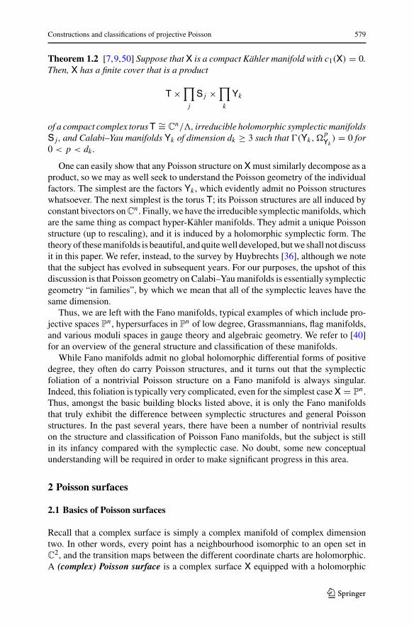
Theorem 1.2 [7,9,50] Suppose that X is a compact Kähler manifold with c1(X) = 0.Then, X has a finite cover that is a product

T ×∏

j

S j ×∏

k

Yk

of a compact complex torusT ∼= Cn/�, irreducible holomorphic symplectic manifolds

S j , and Calabi–Yau manifolds Yk of dimension dk ≥ 3 such that �(Yk,�pYk

) = 0 for0 < p < dk.

One can easily show that any Poisson structure onXmust similarly decompose as aproduct, so we may as well seek to understand the Poisson geometry of the individualfactors. The simplest are the factors Yk , which evidently admit no Poisson structureswhatsoever. The next simplest is the torus T; its Poisson structures are all induced byconstant bivectors onC

n . Finally, we have the irreducible symplecticmanifolds, whichare the same thing as compact hyper-Kähler manifolds. They admit a unique Poissonstructure (up to rescaling), and it is induced by a holomorphic symplectic form. Thetheoryof thesemanifolds is beautiful, andquitewell developed, butwe shall not discussit in this paper. We refer, instead, to the survey by Huybrechts [36], although we notethat the subject has evolved in subsequent years. For our purposes, the upshot of thisdiscussion is that Poisson geometry on Calabi–Yaumanifolds is essentially symplecticgeometry “in families”, by which we mean that all of the symplectic leaves have thesame dimension.

Thus, we are left with the Fano manifolds, typical examples of which include pro-jective spaces P

n , hypersurfaces in Pn of low degree, Grassmannians, flag manifolds,

and various moduli spaces in gauge theory and algebraic geometry. We refer to [40]for an overview of the general structure and classification of these manifolds.

While Fano manifolds admit no global holomorphic differential forms of positivedegree, they often do carry Poisson structures, and it turns out that the symplecticfoliation of a nontrivial Poisson structure on a Fano manifold is always singular.Indeed, this foliation is typically very complicated, even for the simplest caseX = P

n .Thus, amongst the basic building blocks listed above, it is only the Fano manifoldsthat truly exhibit the difference between symplectic structures and general Poissonstructures. In the past several years, there have been a number of nontrivial resultson the structure and classification of Poisson Fano manifolds, but the subject is stillin its infancy compared with the symplectic case. No doubt, some new conceptualunderstanding will be required in order to make significant progress in this area.

2 Poisson surfaces

2.1 Basics of Poisson surfaces

Recall that a complex surface is simply a complex manifold of complex dimensiontwo. In other words, every point has a neighbourhood isomorphic to an open set inC2, and the transition maps between the different coordinate charts are holomorphic.

A (complex) Poisson surface is a complex surface X equipped with a holomorphic

123

580 B. Pym

Poisson bracket as in Definition 1.1. In this section, we will examine the local andglobal behaviour of Poisson structures on surfaces. In the end, we will arrive at thefull birational classification: a relatively short list of Poisson surfaces from which allothers can be obtained by simple modifications, known as blowups.

2.1.1 Local structure

To warm up, let us consider the local situation of a Poisson bracket defined in aneighbourhood of the origin in C

2. Using the standard coordinates x, y on C2, we can

write

{x, y} = f (x, y)

where f is a holomorphic function. The corresponding bivector field is given by

π = f ∂x ∧ ∂y .

Thus, once we have fixed our coordinates, the Poisson bracket is determined by thesingle function f . Because of the dimension, this bivector automatically satisfies[π, π ] = 0, so the Jacobi identity does not impose any constraints on the function f .

Away from the locus where f vanishes, we can invert π to obtain a symplectictwo-form

ω = dx ∧ dy

f.

Applying the holomorphic version of Darboux’s theorem, we may find local holomor-phic coordinates p and q in which

ω = dp ∧ dq,

or equivalently

π = ∂q ∧ ∂p.

Thus, the local structure of π is completely understood in this case.But things are more complicated near the zeros of f . Without loss of generality,

let us assume that f vanishes at the origin. Recall that the zero locus of a singleholomorphic function always has complex codimension one. Hence, if f (0, 0) = 0,there must actually be a whole complex curve D ⊂ C

2, passing through the origin, onwhich f vanishes. Let us suppose for simplicity that f is a polynomial. Then, it willhave a factorization into a finite number of irreducible factors:

f = f k11 f k2

2 · · · f knn .

Therefore, D will be a union of the vanishing sets D1, . . . ,Dn of f1, . . . , fn , the so-called irreducible components. (If f is not polynomial, then D may have an infinite

123


(a) (b)

(c) (d)

Fig. 1 Zero loci of Poisson structures on C2; the dashed line indicates the presence of a component with

multiplicity two. a x ∂x ∧ ∂y , b xy ∂x ∧ ∂y , c (x3 − y2) ∂x ∧ ∂y , d x2(y − x2) ∂x ∧ ∂y

number of irreducible components, but the number of components will be locallyfinite, i.e. there will only be finitely many in a given compact subset of C

2.) Severalexamples of Poisson structures and the corresponding curves are shown in Fig. 1; thesepictures represent real two-dimensional slices of the four-dimensional space C

2.If two bivectors π and π ′ have the same zero set, counted with multiplicities, then

they must differ by an overall factor

π = gπ ′,

where g is a nonvanishing holomorphic function. While the behaviour of these twobivectors is clearly very similar, they will not, in general, be isomorphic, i.e. we cannot take one to the other by a suitable coordinate change on C

2. Here is a simpleexample:

Exercise 2.1 Given any constant λ ∈ C, define a Poisson bracket on C2 by the formula

{x, y}λ = λ xy, (1)

where x, y are the standard coordinates on C2. Show that the brackets {·, ·}λ and

{·, ·}λ′ are isomorphic if and only if λ = ±λ′. Conclude that the isomorphism class ofa Poisson structure on C

2 depends on more information than just the curve on whichit vanishes. �

123

582 B. Pym

In fact, the constant λ appearing in (1) is the only additional piece of informationrequired to understand the local structure of the bracket in this case. More precisely,suppose that π is a Poisson structure on a surface X, and that D is the curve onwhich it vanishes. Suppose that p ∈ D is a nodal singular point of D. (This meansthat, in a neighbourhood of p, the curve D consists of two smooth components withmultiplicity one that intersect transversally at p.) Then one can find a constant λ ∈ C,and coordinates x, y centred at p in which the Poisson bracket has the form (1).

In general, finding a local normal form for the bracket in a neighbourhood of asingular point of D can be complicated. The main result in this direction is a theoremofArnold,whichgives a local normal form in the neighbourhoodof a simple singularityof the curve D. Since we shall not need the precise form of the result, we shall omitit. We refer to the original article [3] for details; see also [23, Section 2.5.1] and [46,Section 9.1].

2.2 Poisson structures on the projective plane

We will be mainly concerned with Poisson structures on compact complex surfaces.The most basic example is the projective plane:

P2 = {lines through 0 in C

3} = (C3\{0})/C∗,

where C∗ acts by rescaling. The equivalence class of a point (x, y, z) ∈ C

3\{0} isdenoted by [x : y : z] ∈ P

2, so that

[x : y : z] = [λx : λy : λz]

for all λ ∈ C∗.

Let us examine the possible behaviour of a Poisson bracket on P2, defined by the

global holomorphic bivector

π ∈ �(P2,∧2TP2).

We will determine the behaviour of π in the three standard coordinate charts on P2,

given by the open dense sets

U1 ={[x : y : z] ∈ P

2 | x �= 0}

U2 ={[x : y : z] ∈ P

2 | y �= 0}

U3 ={[x : y : z] ∈ P

2 | z �= 0}

,

For example, the coordinates associated with U1 are given by

u([x : y : z]) = y

xv([x : y : z]) = z

x,

123


giving an isomorphismU1 ∼= C2. Thus, any Poisson bracket onP

2 must be representedin these coordinates by

{u, v} = f

for some holomorphic function f defined on all of C2. In other words, the bivector

has the form

π |U1 = f ∂u ∧ ∂v.

Meanwhile, in the chart U2 we have the coordinates u, v given by

u([x : y : z]) = x

yv([x : y : z]) = z

y.

They are related to the original coordinates by u = u−1 and v = u−1v on the overlapof the charts. We can therefore compute

{u, v} = {u−1, u−1v}= {u−1, u−1}v + u−1{u−1, v}= 0 + u−1 ·

(−u−2{u, v}

)

= −u−3 f (u, v)

= −u3 f (u−1, u−1v).

Thus, taking the Taylor expansion of f , we find

π |U2 =⎛

⎝u3∞∑

j,k=0

a jk u−( j+k)vk

⎞

⎠ ∂u ∧ ∂v

for some coefficients a jk ∈ C. Since π is holomorphic on the whole chart U2, wemust have that a jk = 0 whenever j + k > 3; otherwise, π would have a pole whenu = 0. These constraints are equivalent to requiring that f be a polynomial in u andv of degree at most three.

A similar calculation in the other chart evidently yields the same result.We concludethat a Poisson bracket on P

2 is described in any affine coordinate chart by a cubicpolynomial. Conversely, given a cubic polynomial in an affine chart, we obtain aPoisson structure on P

2.Once again, the zero set D = Zeros(π) determines π up to rescaling by a global

nonvanishing holomorphic function, but now every such function is constant becauseP2 is compact. Converting from the affine coordinates (u, v) to the “homogeneous

coordinates” x, y, z, we arrive at the following

123

584 B. Pym

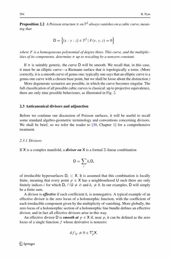
Proposition 2.2 A Poisson structure π on P2 always vanishes on a cubic curve, mean-

ing that

D ={[x : y : z] ∈ P

2 | F(x, y, z) = 0}

where F is a homogeneous polynomial of degree three. This curve, and the multiplic-ities of its components, determine π up to rescaling by a nonzero constant.

If π is suitably generic, the curve D will be smooth. We recall that, in this case,it must be an elliptic curve—a Riemann surface that is topologically a torus. (Morecorrectly, it is a smooth curve of genus one; typically one says that an elliptic curve is agenus one curve with a chosen base point, but we shall be loose about the distinction.)

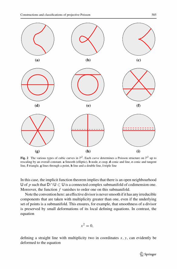
More degenerate scenarios are possible, in which the curve becomes singular. Thefull classification of all possible cubic curves is classical: up to projective equivalence,there are only nine possible behaviours, as illustrated in Fig. 2.

2.3 Anticanonical divisors and adjunction

Before we continue our discussion of Poisson surfaces, it will be useful to recallsome standard algebro-geometric terminology and conventions concerning divisors.We shall be brief, so we refer the reader to [30, Chapter 1] for a comprehensivetreatment.

2.3.1 Divisors

If X is a complex manifold, a divisor on X is a formal Z-linear combination

D =∑

i

kiDi

of irreducible hypersurfaces Di ⊂ X. It is assumed that this combination is locallyfinite, meaning that every point p ∈ X has a neighbourhood U such there are onlyfinitely indices i for which Di ∩ U �= ∅ and ki �= 0. In our examples, D will simplybe a finite sum.

A divisor is effective if each coefficient ki is nonnegative. A typical example of aneffective divisor is the zero locus of a holomorphic function, with the coefficient ofeach irreducible component given by the multiplicity of vanishing. More globally, thezero locus of a holomorphic section of a holomorphic line bundle defines an effectivedivisor, and in fact all effective divisors arise in this way.

An effective divisor D is smooth at p ∈ X if, near p, it can be defined as the zerolocus of a single function f whose derivative is nonzero:

d f |p �= 0 ∈ T∗pX.

123


(a) (b) (c)

(d) (e) (f)

(g) (h) (i)

Fig. 2 The various types of cubic curves in P2. Each curve determines a Poisson structure on P

2 up torescaling by an overall constant. a Smooth (elliptic), b node, c cusp, d conic and line, e conic and tangentline, f triangle, g lines through a point, h line and a double line, i triple line

In this case, the implicit function theorem implies that there is an open neighbourhoodU of p such thatD∩U ⊂ U is a connected complex submanifold of codimension one.Moreover, the function f vanishes to order one on this submanifold.

Note the conventionhere: an effective divisor is never smooth if it has any irreduciblecomponents that are taken with multiplicity greater than one, even if the underlyingset of points is a submanifold. This ensures, for example, that smoothness of a divisoris preserved by small deformations of its local defining equations. In contrast, theequation

x2 = 0,

defining a straight line with multiplicity two in coordinates x, y, can evidently bedeformed to the equation

123

586 B. Pym

x(x + εy) = 0,

for ε ∈ C. For ε �= 0, this deformed divisor has a singular point where the two linesx = 0 and x + εy = 0 meet.

2.3.2 Anticanonical divisors

Recall that on any complex manifold, whatever the dimension, the canonical linebundle is the top exterior power of the cotangent bundle:

KX = det T ∨X = ∧dimXT ∨

X

So, the sections of KX are holomorphic differential forms of top degree. The anti-canonical bundle K−1

X = det TX is the dual of the canonical bundle.

Definition 2.3 A divisor D on X that may be obtained as the zero locus of a sectionof K−1

X is called an (effective) anticanonical divisor.

When X is a surface, we have that

K−1X = ∧2TX,

so that a Poisson structure π on X is simply a section of the anticanonical bundle.Hence, up to rescaling by a constant, a Poisson structure on a compact surface X isdetermined by an anticanonical divisor on X. We can then rephrase Proposition 2.2as follows: an effective divisor on P

2 is an anticanonical divisor if and only if it is acubic curve.

2.3.3 Adjunction on Poisson surfaces

We saw in Sect. 2.2 that a smooth anticanonical divisor in P2 is always an elliptic

curve. We shall now explain a geometric reason why this must be the case. It is aspecial case of a general result, known as the adjunction formula, which relates thecanonical bundle of a hypersurface to the canonical bundle of the ambient manifold(see, e.g. [30, p. 146–147]).

Let (X, π) be a Poisson surface, and let D = Zeros(π) be the correspondinganticanonical divisor. Suppose that p is a point of D. Then π has a well-definedderivative at p, giving an element

dpπ ∈ T∨pX ⊗ ∧2TpX

where TpX is the tangent space of X at p and T∨pX is the cotangent space. (This tensor

is the one-jet of π at p.)Notice that there is a natural contraction map

T∨pX ⊗ ∧2TpX → TpX,

123


given by the interior product of covectors and bivectors. Applying this contraction todpπ , we obtain an element Z p ∈ TpX, and allowing p to vary, we obtain a section

Z ∈ �(D, TX|D)

If x and y are local coordinates on X, then π = f ∂x ∧ ∂y for a function f . We thencompute

dπ = d f ⊗ ∂x ∧ ∂y |D,

so that

Z = ((∂x f )∂y − (∂y f )∂x

) |D.

From this expression, we immediately obtain the following

Proposition 2.4 The vector Z p is nonzero if and only if D is smooth at p. In this case,it is tangent to D, giving a basis for the one-dimensional subspace TpD ⊂ TpX.

Proof The point p ∈ D is smooth if and only if d f |p is nonzero, where f is a localdefining equation for D. It is evident from the local calculation above that this isequivalent to the condition Z p �= 0. It is also easy to see that Z p( f ) = 0, but this isexactly the condition for Z p to be tangent to D. �

Using the fact that elliptic curves are the only compact complex curves whosetangent bundles are trivial, we obtain the following consequence.

Corollary 2.5 If D is smooth, then the derivative of the Poisson structure induces anonvanishing vector field

Z ∈ �(D, TD)

In particular, if D is smooth and compact, then every connected component of D is anelliptic curve.

Definition 2.6 The vector field Z ∈ �(D, TD) is called the modular residue of thePoisson structure π .

Remark 2.7 When D is singular, we can still make sense of vector fields on D asderivations of functions (see Sect. 4.1). In this way, one can make sense of the modularresidue even at the singular points.

2.4 Poisson structures on ruled surfaces

We now describe some more examples of compact complex surfaces. We recall that asurface X is (geometrically) ruled if it is the total space of a P

1-bundle over a smoothcompact curve Y. This is equivalent to saying that X = P(E) is the projectivization

123

588 B. Pym

of a rank-two holomorphic vector bundle E on Y. Not every ruled surface carries aPoisson structure, but there are several that do. In this section, we will describe theirclassification.

As is standard in algebraic geometry, we make no notational distinction between aholomorphic vector bundle and its locally free sheaf of holomorphic sections. Thus,for example, OY denotes both the sheaf of holomorphic functions, and the trivial linebundle Y × C → Y.

2.4.1 Compactified cotangent bundles

The cotangent bundle of any smooth curve is a symplectic surface. It can be compact-ified to obtain a Poisson ruled surface in several ways, which we now describe.

Simplest version: To begin, suppose that Y is a smooth compact curve. Then, wemay compactify the cotangent bundle by adding a point at infinity in each fibre.More precisely, we consider the rank-two bundle E = T ∨

Y ⊕ OY. Its projectivizationX = P(T ∨

Y ⊕OY) has an open dense subset isomorphic to T ∨Y given by the embedding

i : T ∨Y → P(T ∨

Y ⊕ OY)

α �→ span (α, 1).

Its complement is the locus

S = {[∗ : 0] ∈ P(T ∨Y ⊕ OY)},

obtainedby taking the point at infinity in eachP1-fibre. Thus,Sprojects isomorphically

to Y, giving a section of the P1-bundle—the “section at infinity”.

Using local coordinates, it is easy to see that the Poisson structure on T ∨Y extends

to all of X. Indeed, if y is a local coordinate on Y and x = ∂y is the correspondingcoordinate on the fibres of T ∨

Y , then the bivector has the standard Darboux formπ = ∂x ∧ ∂y . Switching to the coordinate z = x−1 at infinity in the P

1 fibres, we find

π = −z2∂z ∧ ∂y .

Thus π gives a Poisson structure on X whose anticanonical divisor is given by

Zeros(π) = 2S ⊂ X,

the section at infinity taken with multiplicity two.

Twisting by a divisor: We can modify the previous construction by introducing a non-trivial effective divisor D on the compact curve Y, i.e. a collection of points in Y withpositive multiplicities. This modification yields a compactification of the cotangentbundle of the punctured curve U = Y\D, as follows.

123


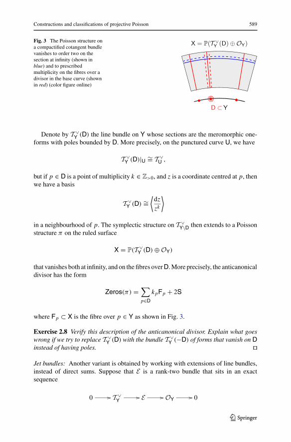
Fig. 3 The Poisson structure ona compactified cotangent bundlevanishes to order two on thesection at infinity (shown inblue) and to prescribedmultiplicity on the fibres over adivisor in the base curve (shownin red) (color figure online)

D ⊂Y

X = P( ∨Y (D) ⊕ OY)

Denote by T ∨Y (D) the line bundle on Y whose sections are the meromorphic one-

forms with poles bounded by D. More precisely, on the punctured curve U, we have

T ∨Y (D)|U ∼= T ∨

U ,

but if p ∈ D is a point of multiplicity k ∈ Z>0, and z is a coordinate centred at p, thenwe have a basis

T ∨Y (D) ∼=

⟨dz

zk

⟩

in a neighbourhood of p. The symplectic structure on T ∨Y\D then extends to a Poisson

structure π on the ruled surface

X = P(T ∨Y (D) ⊕ OY)

that vanishes both at infinity, and on the fibres overD.More precisely, the anticanonicaldivisor has the form

Zeros(π) =∑

p∈DkpFp + 2S

where Fp ⊂ X is the fibre over p ∈ Y as shown in Fig. 3.

Exercise 2.8 Verify this description of the anticanonical divisor. Explain what goeswrong if we try to replace T ∨

Y (D) with the bundle T ∨Y (−D) of forms that vanish on D

instead of having poles. �

Jet bundles: Another variant is obtained by working with extensions of line bundles,instead of direct sums. Suppose that E is a rank-two bundle that sits in an exactsequence

0 �� T ∨Y

�� E �� OY �� 0

123

590 B. Pym

but does not split holomorphically as a direct sum: E �= T ∨Y ⊕ OY. In fact, there is

only one such bundle E on Y, up to isomorphism; it can be realized explicitly as

E = J 1L ⊗ L∨

where L is any line bundle of nonzero degree and J 1L is its bundle of one-jets. (Inother words, E is the dual of the Atiyah algebroid of L.) The uniqueness follows fromthe description of extensions of vector bundles in terms of Dolbeault cohomology(see [30, Section 5.4]). In this case, extensions of OY by T ∨

Y are parametrized byH1(Y, T ∨

Y

) ∼= H2(Y, C), which is one dimensional.The projectivization X = P(E) has a symplectic open set, corresponding to the

vectors in E that project to 1 ∈ OY (an affine bundle modelled on the cotangentbundle T ∨

Y ). Once again, we obtain a Poisson structure on X that vanishes to ordertwo on the section at infinity.

One could try to generalize this construction by introducing a nonempty divisor Don Y and considering extensions

0 �� T ∨Y (D) �� E �� OY �� 0.

However, such extensions are parametrized by the vector spaceH1(Y, T ∨

Y (D)), which

by Serre duality is dual toH0(Y,OY(−D)), the space of global holomorphic functionson Y that vanish on D. Since every global holomorphic function on Y is constant, thisvector space is trivial. We conclude that the extension is also trivial, i.e. we have asplitting E ∼= T ∨

Y (D) ⊕ OY as previously considered, so the construction does notproduce anything new.

2.4.2 Relationship with co-Higgs fields

Let us now consider a general ruled surface X = P(E) over Y. Let ρ : X → Y be thebundle projection. There is an exact sequence

0 �� TX/Y �� TX �� ρ∗TY �� 0,

where TX/Y ⊂ TX is the relative tangent sheaf, i.e. the sheaf of vector fields that aretangent to the fibres. Taking determinants, we find

K−1X

∼= ∧2TX ∼= ρ∗TY ⊗ TX/Y. (2)

In particular, if f ∈ OY, then the Hamiltonian vector field of ρ∗ f is tangent to thefibres of ρ. Thus, for each p ∈ X, we obtain a linear map

T∨pY → �(Fp, TFp )

sending a covector at p to the corresponding vector field on the fibre Fp. Evidently,this linear map completely determines π along Fp.

123


Now since Fp ∼= P(Ep) is a copy of P1, the space �(Fp, TFp ) of vector fields

on the fibre is three dimensional. (In an affine coordinate z on the fibre, the vectorfields ∂z, z∂z and z2∂z give a basis.) Hence, as p varies, these spaces assemble into arank-three vector bundle over Y—the so-called direct image ρ∗TX/Y. In this way, wesee that a Poisson structure on the surface X is equivalent to a vector map bundle mapT ∨Y → ρ∗TX/Y on the curve Y.This is a bit abstract, but fortunately the bundle ρ∗TX/Y has amore concrete descrip-

tion. Indeed, if we think of endomorphisms of E as infinitesimal symmetries, then weget an identification

ρ∗TX/Y∼= End0(E)

where End0(E) is the bundle of traceless endomorphisms of E . The zeros of a vectorfield are identified with the points in P(E) determined by the eigenspaces of thecorresponding endomorphism.

We therefore arrive at the following

Theorem 2.9 Let X = P(E) be the projectivization of a rank-two bundle E over asmooth curve Y. Then, we have a canonical isomorphism

�(X,∧2TX) ∼= �(Y, TY ⊗ End0(E)),

so that Poisson structures on X are in canonical bijection with bundle maps T ∨Y →

End0(E) on Y.

Example 2.10 Suppose that Y is a smooth curve of genus one, i.e. an elliptic curve,and let Z ∈ �(TY) be a nonzero vector field on Y. Let L be a line bundle on Y, andconsider the rank-two bundle E = OY ⊕ L. Let φ0 be the endomorphism of E thatacts by +1 on OY and by −1 on L, so that φ0 is traceless. Therefore, the sectionφ = Z ⊗φ0 ∈ �(Y, TY ⊗End0(E)) defines a Poisson structure π on X = P(E). SinceOY and L are the eigenspaces of φ0, the corresponding sections S0,S1 ⊂ X give thezero locus of the Poisson structure, i.e. Zeros(π) = S0 +S1 ⊂ X is the union of twodisjoint copies of Y. � Exercise 2.11 Let ρ : X = P(E) → Y be a ruled surface, and let π be the Poissonstructure on X corresponding to a section φ ∈ �(Y, TY ⊗ End0(E)). Let D ⊂ Y bethe divisor of zeros of φ. By considering the relation between the zeros of π and theeigenspaces of φ, show that

Zeros(π) = B + π−1(D)

where B ⊂ X is a divisor that meets each fibre of ρ in a pair of points, counted withmultiplicity. �

As a brief digression from surfaces, let us remark that this construction of Poissonstructures on P

1-bundles can be extended to the higher-dimensional setting; see [53,Section 6] for details. In short, the data one needs are a Poisson structure on the baseY

123

592 B. Pym

and a “Poisson module” structure on the bundle E . The latter is essentially an action ofthe Lie algebra (OY, {·, ·}) on the sections of E by Hamiltonian derivations. When thePoisson structure on Y is identically zero, it boils down to the following construction:

Exercise 2.12 Let Y be a manifold, and let E be a rank-two bundle on Y. Arguing asabove, we see that a section φ ∈ �(Y, TY ⊗ End0(E)) defines a bivector field π onX = P(Y), but the integrability condition [π, π ] = 0 is not automatic if dimY > 1.Show that π is integrable if and only if φ is a co-Higgs field [34,61], meaning that

[φ ∧ φ] = 0 ∈ ∧2TY ⊗ End(E),

where [− ∧ −] combines the wedge product TY × TY → ∧2TY and the commutator[−,−] : End(E) × End(E) → End(E). �

2.4.3 Classification of ruled Poisson surfaces

We are now in a position to state the classification of Poisson structures on ruledsurfaces:

Theorem 2.13 (Bartocci–Macrí [6], Ingalls [38]) If (X, π) is a compact Poisson sur-face ruled over a curve Y of genus g, then it falls into one of the following classes:

• g is arbitrary and (X, π) is a compactified cotangent bundle as in Sect. 2.4.1.• g = 1, and (X, π) comes from the construction in Example 2.10.• g = 0 and X = P(OP1 ⊕ O1

P(k)) with k ≥ 0. See [38, Lemma 7.11] for a

description of the possible anticanonical divisors in this case.

We shall not give the full proof here, but let us give an idea of why it is true byexplaining one of its corollaries

Corollary 2.14 A Poisson surface (X, π) ruled over a curve Y of genus at least twomust be a compactified cotangent bundle.

Proof Let X = P(E) for a rank-two bundle on Y. By Theorem 2.9, the Poissonstructure corresponds to a section φ ∈ TY ⊗ End0(E). Let us view φ as a map

φ : E → E ⊗ TY.

Its determinant gives a map

det φ : det E → det(E ⊗ TY) ∼= det E ⊗ (TY)⊗2,

or equivalently a section

det φ ∈ �(Y, (TY)⊗2).

But for a curve Y of genus at least two, the bundle (TY)⊗2 has negative degree, andhence it admits no nonzero sections. Therefore, det φ = 0 identically, and since φ isalso traceless, it must be nilpotent.

123


Now let L ⊂ E be the kernel of φ; it is a line subbundle. (This is obvious awayfrom the zeros of φ, but one can check that it extends uniquely over the zeros as well.)We have an exact sequence

0 �� L �� E �� E/L �� 0, (3)

and because of the nilpotence, φ induces a map E/L → L ⊗ TY which determines itcompletely.

Since the projective bundle P(E) is unchanged if we tensor E by a line bundle,we may tensor (3) by the dual of E/L and assume without loss of generality thatE/L ∼= OY. Then, φ is determined by a bundle mapOY → L⊗TY which may vanishon a divisor D ⊂ Y. This gives a canonical identification L ∼= T ∨

Y (D), so that E fits inan exact sequence

0 �� T ∨Y (D) �� E �� OY �� 0,

from which the statement follows easily. �

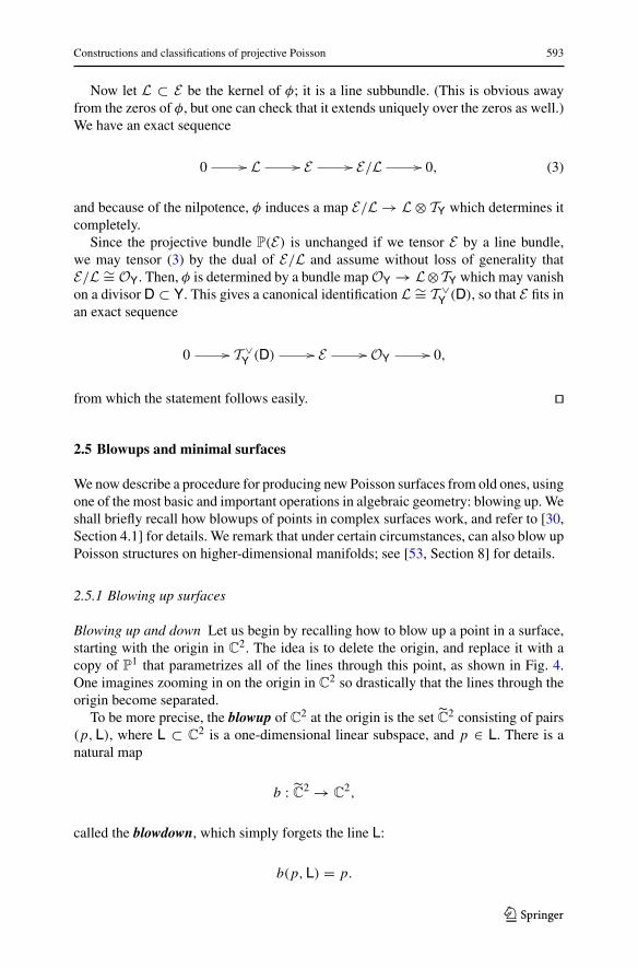
2.5 Blowups and minimal surfaces

We now describe a procedure for producing new Poisson surfaces from old ones, usingone of the most basic and important operations in algebraic geometry: blowing up.Weshall briefly recall how blowups of points in complex surfaces work, and refer to [30,Section 4.1] for details. We remark that under certain circumstances, can also blow upPoisson structures on higher-dimensional manifolds; see [53, Section 8] for details.

2.5.1 Blowing up surfaces

Blowing up and down Let us begin by recalling how to blow up a point in a surface,starting with the origin in C

2. The idea is to delete the origin, and replace it with acopy of P

1 that parametrizes all of the lines through this point, as shown in Fig. 4.One imagines zooming in on the origin in C

2 so drastically that the lines through theorigin become separated.

To be more precise, the blowup of C2 at the origin is the set C

2 consisting of pairs(p,L), where L ⊂ C

2 is a one-dimensional linear subspace, and p ∈ L. There is anatural map

b : C2 → C

2,

called the blowdown, which simply forgets the line L:

b(p,L) = p.

123

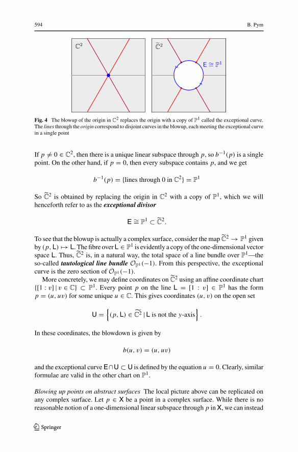
594 B. Pym

Fig. 4 The blowup of the origin in C2 replaces the origin with a copy of P

1 called the exceptional curve.The lines through the origin correspond to disjoint curves in the blowup, each meeting the exceptional curvein a single point

If p �= 0 ∈ C2, then there is a unique linear subspace through p, so b−1(p) is a single

point. On the other hand, if p = 0, then every subspace contains p, and we get

b−1(p) = {lines through 0 in C2} = P

1

So C2 is obtained by replacing the origin in C

2 with a copy of P1, which we will

henceforth refer to as the exceptional divisor

E ∼= P1 ⊂ C

2.

To see that the blowup is actually a complex surface, consider the map C2 → P

1 givenby (p,L) �→ L. The fibre overL ∈ P

1 is evidently a copy of the one-dimensional vectorspace L. Thus, C

2 is, in a natural way, the total space of a line bundle over P1—the

so-called tautological line bundle OP1(−1). From this perspective, the exceptionalcurve is the zero section of OP1(−1).

More concretely, we may define coordinates on C2 using an affine coordinate chart

{[1 : v] | v ∈ C} ⊂ P1. Every point p on the line L = [1 : v] ∈ P

1 has the formp = (u, uv) for some unique u ∈ C. This gives coordinates (u, v) on the open set

U ={(p,L) ∈ C2 |L is not the y-axis

}.

In these coordinates, the blowdown is given by

b(u, v) = (u, uv)

and the exceptional curveE∩U ⊂ U is defined by the equation u = 0. Clearly, similarformulae are valid in the other chart on P

1.

Blowing up points on abstract surfaces The local picture above can be replicated onany complex surface. Let p ∈ X be a point in a complex surface. While there is noreasonable notion of a one-dimensional linear subspace through p inX, we can instead

123


consider lines in the tangent space TpX. The set of one-dimensional subspaces of TpXforms a projective line

E = P(TpX) ∼= P1.

The blowup of X at p is then the surface X that is obtained by replacing p with thecurve E. Thus, as a set, we have

X = (X\{p}) E.

The blowdown map

b : X → X

is the identity map on X\{p}, but contracts the whole exceptional curve to p:

b(E) = {p}

Using local coordinates at p, our calculations on C2 above can be used to give X the

structure of a complex surface. Thus, a tubular neighbourhood of E ∼= P1 in X is

isomorphic to a neighbourhood of the zero section in the line bundle OP1(−1).The surface X, being isomorphic to X away from p, is only slightly more compli-

cated than X itself. For example, one can use a Mayer–Vietoris argument to computethe homology groups:

Proposition 2.15 If X is the blowup of X, with exceptional curve E ⊂ X, then itshomology groups are given by

Hi (X, Z) ={Hi (X, Z) i �= 2

H2(X, Z) ⊕ Z · [E] i = 2.

Blowing down There is also a method for deciding when a given surface Y can beobtained as the blowup of another surface. The idea is to characterize the curvesE ⊂ Ythat are candidates for the exceptional divisor of a blowup. First of all, by construction,such a curve must be isomorphic to P

1. The standard nomenclature for such a curveis as follows:

Definition 2.16 A smooth rational curve is a complex manifold that is isomorphicto the projective line P

1.

As we have seen, the rational curves that arise as exceptional curves in a surface areembedded in a special way. Namely, they have a tubular neighbourhood isomorphic tothe zero section in the tautological line bundle over P

1. This motivates the followingdefinition:

Definition 2.17 A (−1)-curve on a surfaceY is a smooth rational curveE ⊂ Y havingone (and hence all) of the following three equivalent properties:

123

596 B. Pym

1. The normal bundle of E ∼= P1 is isomorphic to the tautological line bundle

OP1(−1).2. The degree of the normal bundle of E is equal to −1.3. The self-intersection number of E is [E] · [E] = −1.

Here, the self-intersection number is defined using the usual topological intersectionpairing on the homology of an orientedmanifold; see e.g. [30, Section 0.4].We remarkthat the equivalence of these three properties is nontrivial. The equivalence of 1 and2 is a consequence of the classification of holomorphic line bundles on P

1 in termsof their degree (e.g. [30, p. 145]). The equivalence of 2 and 3 is a consequence of themore general fact that the self-intersection number of half-dimensional submanifoldis always equal to the integral of the Euler class of its normal bundle.

The following important result explains that these criteria completely characterizethe curves that arise as exceptional divisors of blowups:

Theorem 2.18 (Castelnuovo–Enriques) LetY be a complex surface, and suppose thatE ⊂ Y is a (−1)-curve. Then, there is a surface X and a point p ∈ X such that Y isisomorphic to the blowup X of X at p, and E is identified with the exceptional curvein X.

Proof See [30, Section 4.1]. �

2.5.2 Blowing up Poisson brackets

Blowing up

Suppose now that the surface X carries a Poisson structure π . If p ∈ X, we can formthe blowup X and we might ask whether X inherits a Poisson structure as well. Moreprecisely, we have the blowdown map

b : X → X,

and we ask whether there exists a Poisson structure on X such that b is a Poisson map,i.e. we ask that

b∗{ f, g} = {b∗ f, b∗g}

for all functions f, g ∈ OX. Since b is an isomorphismover an open dense set, there canbe at most one Poisson structure on Xwith this property. Hence, the question is simplywhether the Poisson structure on X\E ∼= X\{p} may be extended holomorphically toX.

Clearly, the answer depends only on the local behaviour of the Poisson structurein a neighbourhood of p, so we can work in local coordinates x, y centred at p, andwrite

123


{x, y} = f (x, y)

for a holomorphic function f .Let us choose corresponding coordinates u, v on the blowup as above, so that

b∗x = u b∗y = uv.

In particular,

v = b∗(x−1y)

In order for the bracket to extend to the blowup, we need to ensure that {u, v} isholomorphic in the whole coordinate chart u, v. We compute

{u, v} = {b∗x, b∗(x−1y)}= b∗{x, x−1y}= b∗(x−1 f (x, y))

= u−1 f (u, uv)

= u−1( f (0, 0) + ug(u, v))

where g is holomorphic near the locus u = 0, i.e. the along the exceptional curve E.So in order for {u, v} to be holomorphic along E, it is necessary and sufficient thatf (0, 0) = 0. In other words, the bivector π on X must vanish at the point p that wehave blown up. Evidently, the calculation is identical in the other coordinate chart onthe blowup, and so we arrive at the

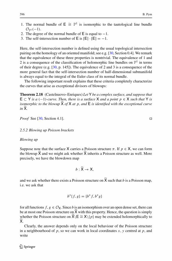
Proposition 2.19 Let (X, π) be a Poisson surface, let p ∈ X be a point in X and let Xbe the blowup of X at p. Then, X carries a Poisson structure π such that the blowdownmap b : X → X is Poisson if and only if π vanishes at p.

Exercise 2.20 Amongst all the possible singularities of a curve in C2, there are three

special classes called A, D and E—the simple singularities [2]. They are the zero setsof the polynomials in the following table:

Ak , k ≥ 1 Dk , k ≥ 4 E6 E7 E8

x2 + yk+1 x2y + yk−1 x3 + y4 x3 + xy3 x3 + y5

Let f be one of these polynomials, and define a Poisson structure π on C2 by

π = f ∂x ∧ ∂y .

Let π be the Poisson structure obtained by blowing up π at the origin in C2. Describe

the divisor D ⊂ C2 on which π vanishes. �

123

598 B. Pym

Blowing down

While blowing up Poisson structures requires some care, blowing them down is mucheasier. In fact, we have the following general result, observed in [53, Proposition 8.4],which shows that holomorphic Poisson structures can often be pushed forward alongmaps. Note that the analogous statement for C∞ manifolds fails dramatically.

Proposition 2.21 Let X be a complex Poisson manifold, and let φ : X → Y be aholomorphic map satisfying one of the following conditions:

1. φ is surjective and proper with connected fibres; or2. φ is an isomorphism away from an analytic subset Z ⊂ Y of codimension at least

two.

Then, there is a unique Poisson structure on Y such that φ is a Poisson map.

Proof Suppose given an open set U ⊂ Y and its preimage φ−1(U) ⊂ X. We need todefine a Poisson bracket on U such that the pullback map

φ∗ : �(U,OU) → �(φ−1(U),Oφ−1(U))

is a morphism of Poisson algebras.We claim that, under our assumptions, φ∗ is already an isomorphism of algebras,

so that this is immediate. Indeed, in the first case, the restriction of any global functionf on φ−1(U) to a fibre is evidently constant, so that f is the pullback of a functionon Y. In the second case, the isomorphism is a consequence of Hartogs’ theorem,which implies that holomorphic functions have unique extensions over codimensiontwo subsets [30, Section 0.1]. � Remark 2.22 What we have really used is the fact that we have an isomorphismφ∗OX

∼= OY of sheaves on Y. � Corollary 2.23 Let X be a complex surface and b : X → X be its blowup at a point.Then, for any Poisson structure on X, there is a unique Poisson structure on X suchthat b is a Poisson map.

2.6 Birational classification of Poisson surfaces

The fact that we can always blow up points on surfaces means that classifying allsurfaces up to isomorphism is likely an intractable task. A more reasonable goal is tofind a list of “minimal” surfaces—surface which are not blowups of other surfaces—and describe the others in terms of these.

Definition 2.24 A compact complex surface isminimal if it contains no (−1)-curves.

Every nonminimal surface can be obtained from a minimal one by a sequence ofblowups. Indeed, suppose that X is a compact surface that is not minimal. Then Xcontains a (−1)-curve which we may blow down to obtain a surface X1. Then, if X1

123


contains a (−1)-curve, we can blow it down to get a surface X2, and so on. Continuingin this way, we produce a sequence of surfaces

X → X1 → X2 → · · · ,

each obtained by blowing down the previous one. We claim that this process must haltafter finitely many steps, yielding a minimal surface Xn . Indeed, one way to see thisis to recall from Proposition 2.15 that blowing down decreases the rank of the secondhomology group. So the rank of the second homology of X gives an upper bound onthe number of blowdowns that we could possibly perform.

One of the major results of 20th century algebraic and complex geometry was acoarse classification of theminimal surfaces into 10 distinct types according to variousnumerical invariants such as Betti numbers—the Enriques–Kodaira classification. Adiscussion of these results would take us too far afield; a detailed treatment can befound, for example in [5], [30, Section 4.5] or [62]. We describe here the classificationof minimal Poisson surfaces. They fall into two broad classes: the symplectic surfacesand the degenerate ones.

2.6.1 Symplectic surfaces

Symplectic surfaces are surfaces equipped with nonvanishing Poisson structures. Inother words, a symplectic surface X admits a nonvanishing section of its anticanonicalline bundle. Thismeans that the anticanonical bundle is trivial, and the space of Poissonstructures on X is one dimensional; they are all constant multiples of one another.

Any compact symplectic surface is automatically minimal. Moreover, since thePoisson structure is nonvanishing, it cannot be blown up to obtain a new Poisson sur-face. The Enriques–Kodaira classification gives a complete list of symplectic surfaces:

Theorem 2.25 A compact complex surface X is symplectic if and only if it is either acomplex torus, a primary Kodaira surface, or a K3 surface.

Complex tori: These are the surfaces that are isomorphic to a quotient C2/�, where

� ∼= Z4 ⊂ C

2 is a lattice of translations; hence, they are topologically equivalentto a four-torus, but different lattices may result in nonisomorphic complex structures.These surfaces are symplectic because the standard Darboux symplectic structure onC2 is invariant under translation, and hence it descends to the quotient. A complex

torus that admits an embedding in projective space is called an abelian variety; theseare characterized by the classical Riemann bilinear relations [30, Section 2.6].

Primary Kodaira surfaces: These are “twisted” versions of complex tori, given byholomorphically locally trivial fibre bundles whose base and fibres are elliptic curves.

K3 surfaces: These are the compact symplectic surfaces that are simply connected.They are all diffeomorphic as C∞ manifolds, but there are many nonisomorphic com-plex structures in this class. One way to produce a K3 surface is to take the zero locus

123

600 B. Pym

in P3 of a homogeneous quartic polynomial, but there are many examples that do not

arise in this way; indeed, many K3 surfaces cannot be embedded in any projectivespace. See [37] for a comprehensive treatment of these surfaces.

2.6.2 Surfaces with degenerate Poisson structures

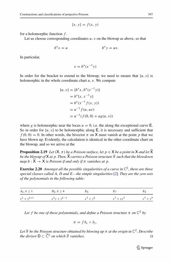
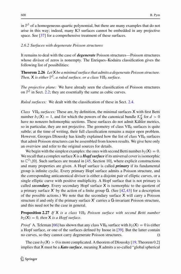
It remains to deal with the case of degenerate Poisson structures—Poisson structureswhose divisor of zeros is nonempty. The Enriques–Kodaira classification gives thefollowing list of possibilities:

Theorem 2.26 LetX be a minimal surface that admits a degenerate Poisson structure.Then, X is either P

2, a ruled surface, or a class VII0 surface.

The projective plane: We have already seen the classification of Poisson structureson P

2 in Sect. 2.2; they are essentially the same as cubic curves.

Ruled surfaces: We dealt with the classification of these in Sect. 2.4.

Class VII0 surfaces: These are, by definition, the minimal surfaces X with first Bettinumber b1(X) = 1, and for which the powers of the canonical bundle Kd

X for d > 0have no nonzero holomorphic sections. These surfaces do not admit Kähler metrics,so in particular, they are not projective. The geometry of class VII0 surfaces is quitesubtle; at the time of writing, their full classification remains a major open problem.However, Georges Dloussky has kindly explained how the list of class VII0 surfacesthat admit Poisson structures can be assembled from known results. We give here onlyan overview and refer to the original sources for details.

Webeginwith the simplest examples: the oneswith secondBetti number b2(X) = 0.We recall that a complex surfaceX is aHopf surface if its universal cover is isomorphicto C

2\{0}. Such surfaces are treated in [45, Section 10], where explicit constructionsand many properties are given. A Hopf surface is called primary if its fundamentalgroup is infinite cyclic. Every primary Hopf surface admits a Poisson structure, andthe corresponding anticanonical divisor is either a disjoint pair of elliptic curves, or asingle elliptic curve with positive multiplicity. A Hopf surface that is not primary iscalled secondary. Every secondary Hopf surface X is isomorphic to the quotient ofa primary surface X′ by the action of a finite group G. (See [42,43] for a descriptionof the possible actions.) We note that the secondary surface X will carry a Poissonstructure if and only if the primary surface X′ carries a G-invariant Poisson structure,and this need not be the case in general.

Proposition 2.27 If X is a class VII0 Poisson surface with second Betti numberb2(X) = 0, then X is a Hopf surface.

Proof A. Teleman [66] has shown that any class VII0 surface with b2(X) = 0 is eithera Hopf surface, or one of the surfaces defined by Inoue in [39]. But the latter containno curves, so they cannot carry degenerate Poisson structures. �

The case b2(X) > 0 ismore complicated. A theorem ofDloussky [19, Theorem 0.2]implies thatXmust be a Kato surface, meaningX admits a so-called “global spherical

123


shell”. More precisely, there is an open set U ⊂ X such that X\U is connected,and U is isomorphic to a tubular neighbourhood of the unit sphere S3 ⊂ C

2. Up toisomorphism, all Kato surfaces may be constructed by an explicit gluing procedureinvolving a germ of a mapping (C2, 0) → (C2, 0). See [18] for a detailed treatment ofthese surfaces; see also [20, Section 2.1] for an overview of the gluing construction.

A Kato surface with b2(X) = n > 0 contains exactly n rational curves Y1, . . . ,Yn .It has an integer-valued topological invariant σn(X) defined by

σn(X) = −n∑

i=1

[Yi ]2 + 2 · (# of curves Yi with a nodal singularity)

where the self-intersection number [Yi ]2 ∈ Z is defined using the intersection pairingon homology. It is known that 2n ≤ σn(X) ≤ 3n. For extremal values of σn(X), theKato surfaces that admit Poisson structures are described as follows (see the citedreferences for details about these surfaces):

Proposition 2.28 Suppose that X is a class VII0 Poisson surface with second Bettinumber b2(X) = n > 0 and anticanonical divisor D ⊂ X.

1. ([18]) If σn(X) = 2n, then X is a compactification of an affine line bundle over anelliptic curve (sometimes called an Inoue surface), and D is the disjoint union ofan elliptic curve and a cycle of rational curves.

2. ([16, Proposition 2.14], [39]) If σn(X) = 3n, then X is an even Inoue–Hirzebruchsurface, and D is the disjoint union of two cycles of rational curves.

On the other hand, if 2n < σn(X) < 3n, then X is called an intermediate Katosurface. In this case, onefirst looks for surfaces that admit a numerically anticanonicaldivisor, i.e. a divisor that arises as the zero locus of a section of a line bundle of theform K−1

X ⊗ L, where L is a line bundle with flat connection. The existence of anumerically anticanonical divisor depends only on discrete invariants of the rationalcurves Y1, . . . ,Yn ⊂ X, namely their intersection matrix ([Yi ] · [Y j ])i, j and theirarithmetic genera; see [17, Lemma 4.2 and Theorem 5.2] for a precise formulation.Moreover, if a numerically anticanonical divisor exists, it is unique.

Now forX to carry a Poisson structure, we need the numerically anticanonical divi-sor to be an actual anticanonical divisor, whichmeans that the flat line bundleLmust betrivial. Such surfaces are special. More precisely, Dloussky [20] has constructed fam-ilies of intermediate Kato surfaces in which every intermediate Kato surface appearsat least once. In these families are strata corresponding to intermediate Kato surfaceswith fixed intersection matrix, and we have the following result:

Proposition 2.29 ([20, Proposition 4.24]) Fix an intersection matrix M of markedintermediate Kato surfaces that admit numerically anticanonical divisors. Inside thefamily of intermediate Kato surfaces with intersection matrix M, the surfaces thatadmit a Poisson structure correspond to a nonempty closed subvariety of codimensionone.

123

602 B. Pym

3 Poisson threefolds

We now turn our attention to three-dimensional Poisson structures. Dimension threeis the lowest in which the integrability condition [π, π ] = 0 for a Poisson structureis nontrivial. Correspondingly, there is a substantial increase in complexity comparedwith Poisson surfaces.

If X is a threefold, we have an isomorphism

∧2TX ∼= �1X ⊗ ∧3TX = �1

X ⊗ K−1X ,

so that bivectors can be alternatively be viewed as one-forms with values in the anti-canonical line bundle. In other words, every bivector field may be written locally asan interior product

π = ιαμ,

where μ ∈ K−1X and α ∈ �1

X. One can easily check that the integrability condition[π, π ] = 0 is equivalent to the equation

α ∧ dα = 0 (4)

that ensures that the kernel of α gives an integrable distribution on X.

Exercise 3.1 Verify this claim. � As was the case for surfaces, the symplectic leaves must all have dimension zero

or two. But now the two-dimensional symplectic leaves are no longer open, and theirbehaviour can be quite complicated; for example, the individual leaves can be densein X. Nevertheless, one can get some very good control over the behaviour and clas-sification of Poisson threefolds.

3.1 Regular Poisson structures

As a warmup, let us consider the simplest class of Poisson threefolds: the regular ones.We recall that a Poisson manifold (X, π) is regular if all of its symplectic leaves havethe same dimension. Equivalently, π is regular if it has constant rank, when viewedas a bilinear form on the cotangent spaces of X.

For a nonzero Poisson structure on a threefold, regularity means that all of theleaves have dimension two, and a theorem of Weinstein [69] implies that the Poissonstructure is locally equivalent to a product C

2 × C where C2 has the standard Poisson

structure ∂x ∧ ∂y and C carries the zero Poisson structure.Clearly, if Y is a symplectic surface and Z is a curve, the product X = Y×Z carries

a regular Poisson structure whose symplectic leaves are the fibres of the projection toZ. Now suppose that X carries a free and properly discontinuous action of a discretegroup G and that the Poisson structure is invariant under the action of G. Then, thequotient X/G will be a new Poisson threefold, and since the quotient map X → X/G

123


is a covering map compatible with the Poisson brackets, it follows that the Poissonstructure on X/G is regular.

In this way, one can easily construct examples of compact Poisson threefolds whoseindividual symplectic leaves are dense submanifolds:

Exercise 3.2 Consider the Poisson structure on C3 ∼= C

2 × C given in coordinatesx, y, z by

π = ∂x ∧ ∂y .

Let � ∼= Z6 ⊂ C

3 be a generic lattice of translations, so that X = C3/� is a compact

six-torus. Determine the conditions under which the symplectic leaves of X will bedense. �

The construction of regular Poisson threefolds from discrete group actions mayseem somewhat simplistic, but in fact all regular projective Poisson threefolds arisein this way. This is guaranteed by the following remarkable and nontrivial theorem ofDruel, which relies on results from the minimal model program for threefolds:

Theorem 3.3 [21] Suppose that (X, π) is a smooth projective Poisson threefold andthat the zero set Zeros(π) ⊂ X is finite. Then, in fact Zeros(π) is empty, so that π

regular. Moreover, (X, π) is isomorphic to a quotient

X ∼= (Y × Z)/G

as above, and it falls into one of the following four classes:

• Y = C2 with the standard Poisson structure, and Z = C. The group G is a lattice

of translations on C2 × C, so that X is an abelian threefold, and the symplectic

leaves are given by (possibly irrational) linear flows.• Y = C

2 and Z = P1. The group G is a lattice of translations on Y, which also acts

on Z by projective transformations. Thus, X is a flat P1-bundle over an abelian

surface; the symplectic leaves are the horizontal sections of the flat connection.• Y is an abelian surface and Z is a compact curve. The group G ⊂ Aut(Z) acts onY × Z by

g · (y, z) = (ug(y) + tg(z), g · z)

where ug ∈ Aut(Y) is a symplectic automorphism of Y that preserves its groupstructure, and tg : Z → Y is a holomorphic map. Thus, X is a symplectic fibrebundle with abelian fibres over an orbifold curve.

• Y is a K3 surface and Z is a compact curve. The action ofG onY×Z is the productof a free action on Z and an action on Y that preserves its symplectic structure.Thus, X is a symplectic fibre bundle with K3 fibres over a smooth curve.

In fact, a similar statement holds in arbitrary dimension. One can deduce from theresults in [49] that if (X, π) is a projective manifold of odd dimension such that π hascorank one away from a codimension-three subset, then actually π is regular. We then

123

604 B. Pym

have the following classification result due to Touzet [67] (see also [22, Section 1]).Note that the proof is independent from Theorem 3.3 and does not rely on the minimalmodel program:

Theorem 3.4 Let (X, π) be a smooth projective Poisson manifold of odd dimension,and suppose that all symplectic leaves of π have codimension one. Then, (X, π) hasa finite covering space (i.e. an étale cover) that is isomorphic to one of the followingtypes of Poisson manifolds:

1. A product T×Y, where T is a complex torus equipped with a translation invariantPoisson structure, and Y is symplectic.

2. A P1-bundle with flat connection over a symplectic manifold Y; the Poisson struc-

ture is the horizontal lift of the symplectic Poisson structure on Y3. A product Y × Z where Z is a curve equipped with the zero Poisson structure and

Y is symplectic.

Remark 3.5 See [22] and [52] for structural results of a similar nature that apply toregular Poisson structures with leaves of codimension two. �

3.2 Poisson structures from pencils of surfaces

We now turn to the case in which the Poisson structure is no longer regular. As inthe regular case, the global behaviour of the two-dimensional leaves may be quitecomplicated. But now there is a second source of difficulty: the Poisson structure mayexhibit very complicated local behaviour, due to the singularities of the foliation inthe neighbourhood of the zero-dimensional leaves.

In this subsection, we consider the special case in which the symplectic leaves liein the level sets of a (possibly meromorphic) function, beginning with the local caseX = C

3.

3.2.1 Jacobian Poisson structures on C3

Let x, y, z be global coordinates onC3, and let f ∈ OC3 be a nonconstant holomorphic

function. Define a bivector by the formula

π = ιd f(∂x ∧ ∂y ∧ ∂z

)

Since d f is closed, this bivector is a Poisson structure by (4). The elementary Poissonbrackets are given by

{x, y} = ∂ f

∂z{y, z} = ∂ f

∂x{z, x} = ∂ f

∂y.

Such a Poisson bracket is called a Jacobian Poisson structure because of its link withthe derivatives of f .

Since the Hamiltonian vector field of f is given by

H f = ιd f π = ιd f ιd f(∂x ∧ ∂y ∧ ∂z

) = 0,

123


we must have that { f, g} = 0 for all functions g, i.e. f is a Casimir function. Putslightly differently, we haveLHg ( f ) = 0, so that f is invariant under all Hamiltonianflows.

Since the Hamiltonian flows sweep out the symplectic leaves, it follows that foreach c ∈ C, the fibre

Yc = f −1(c) ⊂ C3

is a union of symplectic leaves. Because of the dimension, eachYc is a surface, and wecan explicitly describe the symplectic leaves in terms of the geometry of the surfaces,as follows.

First of all, notice that the points in C3 where the Poisson structure vanishes are

precisely the points where d f = 0, i.e. the critical points of f , or equivalently thesingular points of thefibresYc for c ∈ C. Away from these points, the symplectic leaveshave dimension two—the same dimension as the fibres in which they are contained.Hence, they must be open subsets of the fibres. We therefore arrive at the followingdescription of the leaves:

• The zero-dimensional leaves are the singular points of the fibres of f• The two-dimensional leaves are the connected components of the smooth loci ofthe fibres of f .

Example 3.6 Let f = 12 x2 + 2yz. Then, we obtain the linear Poisson brackets

{x, y} = 2y {y, z} = x {z, x} = 2z. (5)

The only critical point of f is the origin, where f has a Morse-type singularity. Thelevel sets of f are the quadric surfaces

12 x2 + 2yz = c (6)

For c �= 0, the level sets are smooth, giving symplectic leaves. But when c = 0, thelevel set is a cone with a singularity at the origin. It is the union of two leaves: theorigin is a zero-dimensional leaf, and the rest of the cone is a two-dimensional leaf.See Fig. 5. � Remark 3.7 The reader may recognize the Poisson brackets (5) as the Lie algebrasl (2, C), and the quadric surfaces (6) as its coadjoint orbits. In fact, if g is any finite-dimensional Lie algebra, then its dual g∨ is a Poisson manifold. More precisely, wehave an inclusion g ⊂ Og∨ as the linear functions, and the Lie bracket on g extendsuniquely to a Poisson bracket on Og∨ . The symplectic leaves of g∨ are exactly thecoadjoint orbits of g. This Poisson structure is often called the Lie–Poisson structureor the Kirillov–Kostant–Souriau Poisson structure. �

Example 3.8 Let f = xyz, so the Poisson brackets are

{x, y} = xy {y, z} = yz {z, x} = zx .

123

606 B. Pym

Fig. 5 Symplectic leaves of theJacobian Poisson structure onC3 defined by the function

f = 12 x2 + 2yz. The red cone is

the level set f −1(0), whosesingular point is the uniquezero-dimensional leaf

Fig. 6 Symplectic leaves of theJacobian Poisson structure onC3 defined by the function

f = xyz. The zero-dimensionalsymplectic leaves are the pointson the coordinate axes. Thetwo-dimensional leaves are thecoordinate planes minus theiraxes (shown in red), and thenonzero level sets of f (shownin blue) (color figure online)

Let us determine the structure of the level sets

xyz = c.

When c �= 0, all three of x, y, z must be nonzero. If we fix x, y ∈ C∗, then z is

uniquely determined as z = cxy . Thus the level set is smooth, giving a symplectic leaf

isomorphic to (C∗)2.On the other hand, the zero level set is given by the equation

xyz = 0,

and is therefore the union of the coordinates planes in C3. This variety is singular

where the planes meet. Thus, the zero-dimensional leaves are given by the coordinateaxes in C

3. Meanwhile, there are three distinct two-dimensional leaves in this fibre,given by taking each plane and removing the corresponding axes. This example isshown in Fig. 6

123


3.2.2 Pencils of symplectic leaves

If X is a compact threefold, it will not admit any nonconstant global holomorphicfunctions, so the construction of Jacobian Poisson structures above will not produceanything nontrivial. However, at least ifX is projective, it will admit many nonconstantmeromorphic functions, and we may try to use those instead. To do so, we need torecall another key algebro-geometric notion: that of a pencil of hypersurfaces (see [30,Section 1.1]).

A meromorphic function can be written locally as

f = g

h

where g and h are holomorphic functions. Notice that f takes on a well-defined valuein P

1 = C ∪ {∞} only at the points where g and h do not both vanish. By removingany common factors of g and h, we can assume that this indeterminacy locus B ⊂ Xis either empty or has codimension two in X. It is called the base locus of f . Wetypically write

f : X �� P1

to indicate that the map f is only well defined away from its base locus (which weleave implicit). It is an example of the more general notion of a rational map.

Given a point t ∈ P1, we can take the fibre of f inX\B. Its closure is a hypersurface

Dt ⊂ X, and the base locus is

B =⋂

t∈P1Dt .

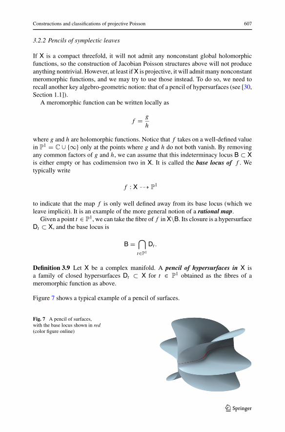
Definition 3.9 Let X be a complex manifold. A pencil of hypersurfaces in X isa family of closed hypersurfaces Dt ⊂ X for t ∈ P

1 obtained as the fibres of ameromorphic function as above.

Figure 7 shows a typical example of a pencil of surfaces.

Fig. 7 A pencil of surfaces,with the base locus shown in red(color figure online)

123

608 B. Pym

Given f : X �� P1 where X is a threefold, we may try to repeat the construction

of the Jacobian Poisson structure in the previous section as follows. Thinking of f asa meromorphic function, consider the meromorphic one-form

α = d log f = d f

f.

We would like to contract this one-form into a trivector in order to obtain a Poissonstructure.

In order for this to work, we have to deal with the poles of α. Considering a localpresentation f = g

h , let us factor g and h into irreducible factors

g = g j10 · · · g jm

m h = hk11 · · · kkn

n ,

so that the irreducible components D0 and D∞ and their multiplicities become appar-ent. Then, we have

α = j1dg1g1

+ · · · + jmdgm

gm− k1

dh1

h1− · · · − kn

dhn

hn.

It is now clear that, even if the fibresD0 andD∞ have components of high multiplicity,the one-form α has only first-order poles. We conclude that the polar divisor of α isthe “reduced divisor”

D = (D0 + D∞)red ⊂ X,

which has all the same irreducible components asD0 +D∞, but with all multiplicitiesset equal to one.

Now suppose thatD is an anticanonical divisor, cut out by a sectionμ ∈ �(X,K−1X ).

If we form the contraction

π = ιαμ,

the zeros of μ will exactly cancel the poles of α, and we will obtain a globally definedholomorphic bivector field on X. Since α is closed, this bivector satisfies [π, π ] = 0and hence we obtain a Poisson structure on X.

The symplectic leaves of π can now be described fairly easily. Each hypersurfaceDt ⊂ X for t ∈ P

1 is a union of symplectic leaves, so every two-dimensional leaf isan open subset of some Dt . Meanwhile, every point in the base locus B = ⋂

t∈P1 Dt

is a zero-dimensional leaf, as are the singular points of the fibres.

Exercise 3.10 Suppose that p ∈ B is a point of the base locus at which D0 and D∞are smooth and transverse. Show that in a suitable system of coordinates x, y, z on Xnear p, the Poisson structure has the form

π = (x∂x + y∂y) ∧ ∂z .

123


Give equations for its symplectic leaves. � This construction of Poisson structures from pencils can be generalized in two

ways: firstly, we can allow the possibility that α has zeros as well as poles, in whichcase we can allow the section ofK−1

X to have poles as well. Secondly, we can considermaps to curves of positive genus instead of P

1; see [53, Section 13] for details.

3.2.3 Poisson structures from pencils on P3

Let us now describe some examples of the above construction in the case whereX = P

3. First of all, we note that every pencil on P3 has the form

f ([x0 : x1 : x2 : x3]) = G(x0, x1, x2, x3)

H(x0, x1, x2, x3)

where G and H are homogeneous polynomials of the same degree. Evidently, thefibres over 0 and ∞ are given by

D0 = Zeros(G) D∞ = Zeros(H).

Now, the anticanonical divisors in P3 are precisely the quartic divisors, just as anti-

canonical divisors in P2 were cubics. We therefore try to arrange so that (D0+D∞)red

is a quartic.

Example 3.11 (Sklyanin [65]) Suppose that G and H are homogeneous quadraticpolynomials. Then, the surfacesD0 andD∞ are quadric surfaces, and so together theyform an anticanonical divisor D = D0 + D∞, giving a Poisson structure π on P

3. IfD0 and D∞ are smooth and transverse, one can use the adjunction formula to showthat the base locus B = D0 ∩ D∞ is a smooth curve of genus one. Thus, π vanisheson an elliptic curve in P

3. To find the remaining zeros of π , we must determine thesingularities of the surfaces in the pencil.

To do so, we use the fact that a pair of homogeneous quadratic forms can alwaysbe put into a normal form. More precisely, there exists homogeneous coordinatesx0, . . . , x3 and constants a0, . . . , a3 ∈ C such that

G = x20 + x21 + x22 + x23 H = a0x20 + a1x21 + a2x22 + a3x23

The surfaces in the pencil are then given by GH = t , or equivalently

λG − μH =3∑

i=0

(λ − μai )x2i = 0

where t = λ−1μ. For generic values of t , the function λG − μH is a nondegeneratequadratic form, and hence its only critical point is the origin in C

4. It follows that thecorresponding surface Dt ⊂ P

3 is smooth.

123

610 B. Pym

However, when t = a−10 , so that λ = −μa0, the quadratic form has rank three, and

this results in an isolated singularity of the surface Dt at the point [1 : 0 : 0 : 0] ∈Dt ⊂ P

3. Similarly, the other values t = a−1i give surfaces with isolated singularities

at [0 : 1 : 0 : 0], [0 : 0 : 1 : 0] and [0 : 0 : 0 : 1].We thus arrive at the following decomposition of P

3 into symplectic leaves:

• The four points S = {[1 : 0 : 0 : 0], . . . , [0 : 0 : 0 : 1]} are isolated symplecticleaves of dimension zero. Near each of these points, one can find coordinates inwhich the Poisson structure takes the form of Example 3.6.

• The base locus B = D0 ∩D∞ is an elliptic curve, and each of its points is a zero-dimensional leaf. Near such a point, the Poison structure is of the type describedin Exercise 3.10.

• The two-dimensional leaves are given by the open sets Dt\(B∪ S) in the quadricsurfaces Dt for t ∈ P

1.

Notice that Zeros(π) has components of dimensions zero and one. � Example 3.12 Similarly, suppose thatG is an irreducible homogeneous cubic functionand that H is linear. Then, we obtain a pencil on P

3 from f = H−3G. Now, we haveD0 = Zeros(G) and D∞ = 3Y where Y ∼= P

2 ⊂ P3 is the plane defined by H = 0.

Thus, the polar divisor of f −1d f is given by

(D0 + D∞)red = D0 + Y,

which is evidently quartic. Hence, we obtain a Poisson structure whose leaves aredetermined by the pencil.

The base locus is the intersection D0 ∩ Y which is a cubic curve. If we assumethat G is sufficiently generic, this curve will be smooth, hence elliptic. There areeight additional isolated points where the Poisson structure vanishes, correspondingto singularities of the surfaces in the pencil. �

3.3 Further constructions

There are a number of other ways in which one can construct Poisson threefolds. Weleave the exploration of these constructions as exercises to the reader.

Closed meromorphic one-forms: Let X be a threefold, and let α be a closed one-formwith poles on an anticanonical divisor D ⊂ X, cut out by the vanishing of a sectionμ ∈ �(X,K−1

X ). Then, ιαμ is a holomorphic Poisson structure. A special case is whenα = d log f for a pencil f as above, but in general the symplectic leaves need not bethe level sets of a meromorphic function.

Exercise 3.13 Let [x0 : x1 : x2 : x3] be homogeneous coordinates on X = P3, and

let D = Zeros(x0x1x2x3) be the union of the coordinate planes (an anticanonicaldivisor). Show that every closed meromorphic one-form with first-order poles on Dmay be written in homogeneous coordinates as

123


α =3∑

j=0

λ jdx j

x j

where λ0, . . . , λ3 ∈ C are constants satisfying∑3

j=0 λ j = 0. Show that the induced

symplectic foliation of P3\D ∼= (C∗)3 is regular, but for generic values of the constants

λ0, . . . , λ3, the leaves are not the level sets of any single-valued function. �

Horizontal lifts: In Exercise 2.12, we saw how to produce Poisson structures on P1-

bundles, where the base is equippedwith the zero Poisson structure. As another specialcase of the general construction in [53, Section 6], we can produce Poisson structureson P

1-bundles over surfaces with nontrivial Poisson structures as follows:

Exercise 3.14 Let (Y, π) be a Poisson surface with degeneracy divisor D ⊂ Y. Sup-pose that E is a rank-two vector bundle on Y equipped with a meromorphic flatconnection

∇ : E → E ⊗ �1Y(D).

By this, we mean that ∇ is a flat connection in the usual sense away from D, but in alocal trivialization near D, it takes the form

∇ = d + f −1A

where A is a holomorphic matrix-valued one-form, and f is a local defining equationfor D. Show that, even though the connection ∇ is singular, the horizontal lift of π

to X = P(E) is holomorphic everywhere, so that X becomes a Poisson threefold.Describe the symplectic leaves. �

Group actions: Let G be a Lie group and let g be its Lie algebra. We recall that aclassical triangular r -matrix for G is a tensor r ∈ ∧2g satisfying [r, r ] = 0 ∈ ∧3g.It corresponds to a left-invariant Poisson structure on G.

Now let X be a manifold equipped with an action of G. Then, we may evidentlypush r forward along the action map g → �(X, TX) to obtain a Poisson structure onX.

Exercise 3.15 Suppose that G is two-dimensional. Then, every r ∈ ∧2g is a classicaltriangular r-matrix. Describe the symplectic leaves of the induced Poisson structureon X in terms of the orbits of G. �

Exercise 3.16 Show that the Poisson structures on P3 described in Exercise 3.13 are

induced by a classical triangular r-matrix for the group G = (C∗)3, where G acts onP3 in the standard way, by rotation of the coordinates. �

123

612 B. Pym

3.4 Poisson structures on P3 and other Fano threefolds

For some simple threefolds X, the space Pois(X) ⊂ �(X,∧2TX) of Poisson structurescan be described explicitly. In particular, the space of Poisson structures on P

3 isquite well understood, thanks to work of Cerveau–Lins Neto [13] and Loray–Pereira–Touzet [48]:

Theorem 3.17 The variety Pois(P3) has six irreducible components, and there areexplicit descriptions of the generic Poisson structures in each component.

We refer to [54, Section 8] and [55] for a detailed description of the geometry ofthese Poisson structures and their quantizations. Let us just remark that the Poissonstructures in each component can be described by constructions that we have alreadyseen: pencils, closed logarithmic one-forms, r -matrices, P

1-bundles, and blowdowns(nowof threefolds instead of surfaces).Moreover, the generic Poisson structure in eachcomponent vanishes on a curve and possibly also a finite collection of isolated points.The six components can be distinguished by the structure of these curves.We note thatthe two components corresponding to smooth curves were classified independentlyby Polishchuk [53]

In fact, the paper [13] of Cerveau and Lins Neto solves a slightly different problem:it gives the classification of certain codimension-one foliations on P

n for n ≥ 3 underthe assumption that the singular set has no divisorial components; when n = 3, thesefoliations coincide with the symplectic foliations of Poisson structures whose zerosets are unions of curves and isolated points. The paper [48] of Loray–Pereira–Touzetgives an alternative approach to the classification of such foliations when n = 3, andcompletes the classification of Poisson structures by showing that the ones with nodivisorial components in their zero sets are Zariski dense in Pois(P3). It also extendsthe result to a classification of Poisson structures on rank-one Fano threefolds:

Theorem 3.18 [48] Let X be a Fano threefold with second Betti number b2(X) = 1.If Pois(X) �= {0}, then X is one of the following manifolds

• The projective space P3

• A quadric or cubic hypersurface X ⊂ P4

• A degree-six hypersurface X ⊂ P(1, 1, 1, 2, 3)• A degree four hypersurface X ⊂ P(1, 1, 1, 1, 2)• An intersection of two quadric hypersurfaces in P

5

• The minimal SL(2, C)-equivariant compactification of SL(2, C) /G, where G <

SL(2, C) is the binary octahedral or icosahedral subgroup.

In each case, there is an explicit list of irreducible components of Pois(X), describedin terms of the constructions mentioned above.

Fano threefolds have been completely classified; see [40] for a summary. To theauthor’s knowledge at the time of writing, the classification of their Poisson structuresis not yet complete. It would be interesting to know whether there are any examplesthat cannot be obtained from the constructions we have discussed.

123


4 Poisson subspaces and degeneracy loci

We now turn our attention to the geometry of higher-dimensional Poisson structures,with an emphasis on the singularities that arise. As we have seen, the locus wherea Poisson bracket vanishes is a key feature of Poisson surfaces and threefolds. Indimension four and higher, it is possible for the Poisson structure to have leaves ofmany different dimensions, and we will want to understand how they all fit together.This typically leads to complicated singularities, so it is helpful begin with a moresystematic treatment of Poisson structures on singular spaces.

4.1 Poisson subspaces and multiderivations

Let us briefly recall the standard notion of an analytic subspace (or subscheme) of acomplex manifold; see [30, Section 5.3] for more details. If X is a complex manifold,then a (closed) complex analytic subspace of X is a closed subspace Y ⊂ X that islocally cut out by a finite collection of holomorphic equations. More precisely, thereis an ideal I ⊂ OX that is locally finitely generated, such that Y is the simultaneousvanishing set of all elements of I.

The holomorphic functions on Y are given by OY = OX/I. Thus, they dependon the ideal I, rather than just the set of points underlying Y. For example, if x isthe standard coordinate on X = C, the ideals (xk) ⊂ OC for different values of kdefine different analytic subspaces with same underlying set Y = {0}; their algebrasof functions are given by OY

∼= C · 1 ⊕ C · x ⊕ · · · ⊕ C · xk−1 with xk = 0.Now suppose that (X, π) is a complex Poisson manifold. An analytic subspace

Y ⊂ X is a Poisson subspace if it inherits a Poisson bracket from the one on X via therestriction map OX → OY. From the definition, we immediately have the following

Lemma 4.1 For a closed analytic subspace Y ⊂ X with ideal sheaf I ⊂ OX, thefollowing are equivalent:

1. Y is a Poisson subspace2. I is a Poisson ideal, i.e. {OX, I} ⊂ I3. I ⊂ OX is invariant under Hamiltonian flows

Example 4.2 If f ∈ OX is a Casimir function, then the level sets of f are all Poissonsubspaces. Shifting f by a constant, it is enough to check this for the zero level set,defined by the ideal ( f ) = OX · f ⊂ OX. Using { f,−} = 0, we compute

{OX,OX · f } = {OX,OX} f + OX{OX, f } = {OX,OX} f ⊂ ( f ),

so that ( f ) is a Poisson ideal, as required. � Exercise 4.3 Show that if Y1,Y2 ⊂ X are Poisson subspaces with ideals I1 and I2,then I1 ∩ I2, I1 · I2 and I1 + I2 are also Poisson ideals. Geometrically, these oper-ations correspond to the union, the union “with multiplicities” and the intersection,respectively. �

123

614 B. Pym

Notice that since a Poisson subspace Y ⊂ X is invariant under all Hamiltonianflows, it is necessarily a union of symplectic leaves. However, the converse need nothold; the main difficulty has to do with the possible existence of nilpotent elements inOY.

Indeed, let us recall that if Y ⊂ X is a closed analytic subspace in an arbitrarycomplex manifold, then the reduced subspace Yred ⊂ Y ⊂ X is the unique analyticsubspace of X that has the same underlying points as Y, but has no nilpotent elementsin its algebra of functions. More precisely, if Y is defined by the ideal I ⊂ OY, thenYred is defined by the radical ideal

√I =

{f ∈ OX | f k ∈ I for some k ∈ Z>0

}

and we have a natural inclusion of subspaces Yred ⊂ Y corresponding to the reverseinclusion I ⊂ √

I of ideals.

Exercise 4.4 Suppose that Z ∈ TX is a vector field on X that is tangent to Y, in thesense that its flow preserves the ideal I, i.e. Z(I) ⊂ I. Show that Z is also tangent toYred. Conclude that if π is a Poisson structure on X such that Y is a Poisson subspace,then Yred is also a Poisson subspace. � Exercise 4.5 Equip X = C

3 with the Poisson brackets

{x, y} = 2y {y, z} = x {z, x} = 2z (7)

from Example 3.6. Find an analytic subspace Y ⊂ X such that Yred is a Poissonsubspace, but Y is not. (Hint: look for a zero-dimensional example.) �

4.2 Vector fields and multiderivations

The tangent spaces of an analytic spaceY do not assemble into a vector bundle over thesingular points, but we can still make sense of vector fields as derivations of functions:

TY = Der(OY).

Clearly, derivations of OY can be added together, and multiplied by elements of OY,and hence they form an OY-module. This module structure is enough for many pur-poses in Poisson geometry and will certainly be sufficient in this paper. But we shouldremark in passing that TY is just a shadow of a richer object known as the “tangentcomplex”, which is also important for understanding the singularities and their defor-mations.

Exercise 4.6 Recall from Example 3.6 that the function f = 12 x2 + 2yz on C

3

generated the Poisson brackets (5) via the Jacobian construction. The zero setY = f −1(0) ⊂ C

3 is an analytic subspace that has an isolated singular point atthe origin. Show that the Hamiltonian vector fields Hx , Hy and Hz, together with theEuler vector field x∂x + y∂y + z∂z , induce derivations of OY that generate TY as anOY-module. �

123


To formulate an analogue of the correspondence between Poisson brackets andbivectors, we recall that amultiderivation of degree k onY is aC-multilinear operator

OY × · · · × OY︸︷︷︸k times

→ OY

that is totally skew-symmetric and is a derivation in each argument. We denote by

X kY = {multiderivations of degree k on Y}

the sheaf of multiderivations; like TY = X 1Y , all these sheaves are OY-modules.

It is straightforward to define a Schouten-type bracket on multiderivations; see,e.g. [46, Chapter 3]. In this way, we see that a Poisson bracket on Y is equivalent to abiderivation π ∈ X 2

Y satisfying the integrability condition [π, π ] = 0 ∈ X 3Y .

From our experience with manifolds, it is tempting to think that a multiderivationshould be the same thing as a section of∧kTY, but this can fail whenY is singular.Moreprecisely, if we interpret ∧kTY as the kth exterior power of TY as anOY-module, thenthere is a natural map∧kTY → X k

Y , defined by sending a wedge product Z1∧· · ·∧ Zk

of vector fields to the multiderivation

( f1, . . . , fk) �→ det(Zi ( f j ))1≤i, j≤k

However, this map will typically fail to be an isomorphism at the singular points ofY. Poisson structures are always elements of X 2

Y , but they may not be defined byelements of ∧2TY. Thus, one should work with X •

Y rather than ∧•TY when doingPoisson geometry on singular spaces.

Example 4.7 We continue Exercise 4.6. Since f is a Casimir function, Y is a Poissonsubspace. We claim that the corresponding biderivation π ∈ X 2

Y is not in the imageof the natural map ∧2TY → X 2

Y .Indeed, by Exercise 4.6, TY is generated by derivations that vanish at the origin.

Therefore, elements of ∧2TY must vanish to order two there. But the Poisson bracketonly vanishes to order one, so it cannot be given by an element of∧2TY.More precisely,let m = (x, y, z) ⊂ OY denote the ideal of functions vanishing at the origin. Then,Z(OY) ⊂ m for any Z ∈ TY. Therefore, for any bivector η ∈ ∧2TY, the correspondingmultiderivation satisfies η(OY ×OY) ⊂ m2. But by definition of the Poisson bracket,we have π(x, y) = 2y /∈ m2. �

4.3 Degeneracy loci

4.3.1 Definition and basic properties

We now turn to a natural class of Poisson subspaces that are key structural features ofany Poisson manifold: the degeneracy loci.

123

616 B. Pym

Let (X, π) be a Poisson manifold, and let k ≥ 0 be an integer. The 2kth degeneracylocus of X is the subset

Dgn2k(π) = {p ∈ X | the symplectic leaf through p has dimension ≤ 2k} .

It is a generalization of the zero locus Dgn0(π) = Zeros(π). Indeed, Dgn2k(π) isprecisely the locus where the tensor π , viewed as a bilinear form on the cotangentspaces, has rank at most 2k. We therefore have the identification

Dgn2k(π) = Zeros(πk+1) πk+1 = π ∧ · · · ∧ π︸︷︷︸k times

∈ ∧2k+2TX.

In local coordinates, the locus Dgn2k(π) is the vanishing set of the Pfaffians of all(2k +2)× (2k +2) skew-symmetric submatrices of the matrix ({xi , x j }i, j ) of Poissonbrackets. In particular, it is an analytic subspace. For a more invariant description ofthis ideal, we can observe that there is a natural map of OX-modules

�2k+2X

πk+1�� OX

given by the pairing of polyvectors and forms. The image of this map is a submodulein OX, hence an ideal; it is the ideal defining Dgn2k(π).

Thus, the degeneracy loci give a filtration of X by closed analytic subspaces

Dgn0(π) ⊂ Dgn2(π) ⊂ Dgn4(π) ⊂ · · · ⊂ X.

One can check that when Dgn2k(π) �= X, the subspace Dgn2k−2(π) ⊂ Dgn2k(π) isalways contained in the singular locus of Dgn2k(π). (This inclusion may or may notbe an equality.) Thus singularities are very common in the study of higher-dimensionalPoisson brackets.

Example 4.8 Let w, x, y, z be global coordinates on C4, and consider the Poisson

structure

π = w ∂w ∧ ∂x + y ∂y ∧ ∂z

The corresponding matrix of Poisson brackets is

⎛

⎜⎜⎝

0 w 0 0−w 0 0 00 0 0 y0 0 −y 0

⎞

⎟⎟⎠

Clearly, π vanishes on the plane w = y = 0, so this plane is the degeneracy locusD0(π). Meanwhile, D2(π) is given by the vanishing of

π2 = 2wy ∂w ∧ ∂x ∧ ∂y ∧ ∂z .

123


Thus,D2(π) is the union of the hyperplanesw = 0 and y = 0, which is singular alongtheir intersection. So in this case, the inclusion Dgn0(π) ⊂ Dgn2(π)sing is actuallyan equality. �

By definition, the locus D2k(π) is a union of symplectic leaves, which suggests thefollowing

Proposition 4.9 ([53, Corollary 2.4]) The degeneracy locus Dgn2k(π) is always aPoisson subspace of X.

Proof Let I be the ideal definingD2k(π) as above.We need to show that I is preservedby the flow of any Hamiltonian vector field Hg for g ∈ OX. But if f ∈ I, then f islocally given by a pairing

f =⟨πk+1, ω

⟩

where ω ∈ �2k+2X . Therefore

{g, f } = LHg f

= LHg

⟨πk+1, ω

⟩

=⟨LHg (π

k+1), ω⟩+⟨πk+1,LHg ω

⟩

=⟨(k + 1)πk ∧ LHg π,ω

⟩+⟨πk+1,LHg ω

⟩

=⟨πk+1,LHg ω

⟩

∈ I

where we have used the fact LHg π = 0. �

4.3.2 Dimensions of degeneracy loci

The study of degeneracy loci of vector bundle maps (also known as determinantalvarieties) is a classical subject in algebraic geometry, and quite a lot is known aboutthem.We recall somebasic facts about degeneracy loci of skew forms; see, e.g. [33,41],for more details.

If E is a vector bundle of rank n and

ρ ∈ �(X,∧2E)

is a skew-symmetric form, then we may define its degeneracy loci Dgn2k(ρ) as wedid for Poisson structures above. In this setting, there is a bound on the codimension

codimDgn2k(ρ) ≤(

n − 2k

2

), (8)

123

618 B. Pym

which can be understood intuitively as follows. Suppose p ∈ X is a point where therank of ρ is equal to 2k. Then, near p we can choose collections of sections e1, . . . , ek ,f1, . . . , fk and g1, . . . , gn−2k that give a basis for E in which ρ takes the form

ρ =k∑

j=1

e j ∧ f j +∑

1≤i< j≤n−2k

hi j gi ∧ g j

where hi j are functions that vanish at p. It is clear that the rank of ρ drops to 2kprecisely where the functions hi j vanish. Since there are n − 2k of these, we get theexpected bound on the codimension. With more effort, one can upgrade this argumentto work at points p ∈ D2k(ρ) where rank ρ < 2k.

When the bound (8) is an equality one has relatively good control over the singu-larities of Dgn2k(ρ) that can occur, as well as formulae for their fundamental classesin the cohomology of X. But when the codimension is smaller than the bound, we arein the situation of excess intersection, and it is rather more difficult to control what ishappening.

One of the interesting features of Poisson structures is that excess intersection isquite common. To see why this must be true, notice that if p is a point where the rankof π is equal to 2k, then the entire symplectic leaf through p clearly lies inDgn2k(π).Hence, the codimension of Dgn2k(π) in a neighbourhood of p at most n − 2k, whichis rather less than (8) would suggest. On the other hand, there are also examples where

codimD2k(π) > n − 2k.

In these situations, there are no leaves of dimension 2k, but there are leaves of dimen-sion less than 2k. Here is an example when k = 1:

Exercise 4.10 Let π be the linear Poisson structure associated with the Lie algebrasl (3, C). Show that Dgn2(π) = Dgn0(π) = {0} as sets. Note that Dgn2(π) is notreduced in this case, so the ideals are different. �

There is an intriguing conjecture concerning the excess dimension of degeneracyloci on compact Poisson varieties.

Conjecture 4.11 (Bondal [10]) Suppose that X is a Fano manifold and π is a Poissonstructure on X. Then, for every k such that 0 ≤ 2k < X, the degeneracy locus D2k(π)

has an irreducible component of dimension ≥ 2k + 1.

Beauville [8] has suggested that the Fano condition could likely be considerablyrelaxed.

The author is unaware of any counterexamples to the conjecture. Indeed, it has beenverified in some special cases. The first main result is the following

Theorem 4.12 ([8, Proposition 4],[53, Corollary 9.2]) Let (X, π) be a compact Pois-son manifold. Suppose that rank(π) = 2k + 2 on an open dense set and that

c1(X)n−2k−1 �= 0.

123


Then, Dgn2k(π) has a component of dimension at least 2k + 1.

In other words, the conjecture always holds for the rank drop locus of maximaldimension. This implies, in particular, that Bondal’s conjecture holds for Fano three-folds. (The three-dimensional case could also be deduced as a consequence of Druel’sclassification Theorem 3.3, but that result is much harder to prove.) The proof is astraightforward application of Bott’s theorem [11], which gives a topological obstruc-tion to the existence of a regular foliation on a manifold, in terms of Chern classes.

The second main result implies that the conjecture holds for Fano fourfolds:

Theorem 4.13 [31] Let (X, π) be a Fano manifold of dimension n = 2d. Then,Dgn2d−2(π) has a component of dimension at least n − 1 and Dgn2d−4(π) has acomponent of dimension at least 2d − 3.

In this case, Bott’s vanishing theorem cannot be directly applied. The proof is basedon some new tools that relate the Poisson geometry of the canonical bundle to thesingularities of the subspace Dgn2d−2(π) ⊂ X.

Another piece of evidence for the conjecture comes from the fact that the adjunctionprocedure described in Sect. 2.3.3 has a natural generalization to the higher degen-eracy loci [31]. Taking the derivative of πk+1 along its zero locus, and applying thecontraction T ∨

X ⊗ ∧2k+2TX → ∧2k+1TX, one produces a modular residue that isa multiderivation of degree 2k + 1 on Dgn2k(π). This residue is nonzero in manyexamples, which hints at a possible deeper geometric explanation for the dimensionsappearing in the conjecture.

5 Log symplectic structures

As the dimension of X increases, the singularities of the degeneracy loci typicallybecomemuchmore complicated. To get some control over the situation, it is helpful tomake some simplifying assumptions. In the past several years, starting with the works[28,32,57], considerable attentionhas beendevoted to the case ofC∞ andholomorphicPoisson structures that have an open dense symplectic leaf, and degenerate in a simpleway along a hypersurface. In this final section, we give an introduction to these “logsymplectic” manifolds, and describe some of the classification results that have beenobtained.

5.1 Definition and examples

Suppose that (X, π) is a Poisson manifold that is generically symplectic, i.e. it has anopen dense symplectic leaf. Then, the dimension n = dimX is necessarily even, andthe maximal degeneracy locus D = Dgnn−2(π) ⊂ X is described by the vanishing ofthe top power

πn/2 ∈ �(X,K−1X ),

i.e. it is an anticanonical divisor in X when it is nonempty.

123

620 B. Pym

Definition 5.1 A generically symplectic Poisson manifold (X, π) is log symplectic ifthe anticanonical divisor D is reduced, i.e. all components have multiplicity one.

When we want to emphasize the degeneracy divisor, we will say that the triple(X,D, π) is a log symplectic manifold.

Exercise 5.2 Let (X, π) be a log symplectic manifold. Show that every irreduciblecomponent of the degeneracy divisor D is a Poisson subspace of X. � Remark 5.3 In fact, a theorem of Seidenberg [64] implies that the irreducible com-ponents of any analytic space or scheme Y are automatically preserved by any vectorfield on Y. This implies that the irreducible components of any Poisson space arealways Poisson subspaces. �

The reason for the terminology “log symplectic” is as follows. Consider the sub-sheaf

TX(− logD) ⊂ TX

consisting of all vector fields tangent toD. Near a smooth point p ∈ D, we can chooselocal coordinates x1, . . . , xn on X such that D = {x1 = 0}. We then have a basis

TX(− logD) ∼= ⟨x1∂x1 , ∂x2 , . . . , ∂xn

⟩

for TX(− logD) as an OX-module. In other words, away from the singular locus,TX(− logD) is the sheaf of sections of a vector bundle. (In general, it may fail to bea vector bundle over the singular locus, but it is the next best thing: a reflexive sheaf,meaning that it is isomorphic to its double dual.)

The dual of TX(− logD) is the sheaf �1X(logD) of differential one-forms with

logarithmic singularities alongD in the sense of [15,63]. In coordinates near a smoothpoint as above, we have a basis

�1X(logD) ∼=

⟨dx1x1

, dx2, . . . , dxn

⟩

and the term “logarithmic” comes from the fact that dx1x1

= d log x1.One can show that the Poisson structure π is log symplectic if and only if the

isomorphism TX\D ∼= �1X\D defined by the symplectic structure on X\D extends to an

isomorphism

TX(− logD) ∼= �1X(logD)

of OX-modules, even over the singular points of D. What this means is that we caninvert π to obtain a logarithmic two-form

ω ∈ �2X(logD)

123


which is called the log symplectic form. Near a smooth point of D, one can find logDarboux coordinates (pi , qi )i=1,...,n/2 so that

ω = dp1p1

∧ dq1 + dp2 ∧ dq2 + · · · + dpn/2 ∧ dqn/2; (9)

see [28,32].Near a singular point, though, the structure can bemuchmore complicated.We recall now several examples of log symplectic manifolds, some of which are

taken from [28].

Example 5.4 (Surfaces) For X = P2, most Poisson structures are log symplectic; the

only cases that are not log symplectic are cases (h) and (i) in Fig. 2, which havecomponents with multiplicity greater than one. In contrast, the Poisson ruled surfacesobtained from compactified cotangent bundles (Sect. 2.4.1) are never log symplectic,since the section at infinity has multiplicity two. � Example 5.5 (Products) If (X,D, π) and (X′,D′, π ′) are log symplectic, then so isthe product (X × X′,D × X′ + X × D′, π + π ′). � Example 5.6 (Hilbert schemes) If (X, π) is a log symplectic surface, then by the previ-ous example Xn carries a log symplectic structure that is invariant under permutationsof the factors. It therefore descends to a Poisson structure on the singular varietyXn/Sn , and this Poisson structure lifts to a log symplectic structure on the naturalresolution of singularities—the Hilbert scheme Hilbn(X). See [59,60] for a discus-sion of these Poisson structures and a proof that they have unobstructed deformations.We remark that a similar construction works when (X, π) is replaced with certainnoncommutative surfaces; see [51,58]. � Example 5.7 (Monopoles) The reduced moduli space of SU(2)-monopoles of chargek is a 2k-dimensional holomorphic symplectic manifold. It has a natural compactifi-cation to a log symplectic structure on P

k−1 × Pk−1; see [4,28]. �

Example 5.8 (Bundles on elliptic curves) In [24,25], Feigin and Odesskii introducedfamilies of Poisson structures qn,r (Y) on P

n−1, determined by an elliptic curve Y andcoprime integers (n, r). These structures are obtained by viewing P

n−1 as a certainmoduli space of bundles over Y, and they exhibit some beautiful classical geometryrelated to the embedding of Y as an elliptic normal curve in P

n−1. For example, thePoisson structure q2d+1,1 on P

2d is log symplectic, and for any k ≥ 0, the degeneracylocus Dgn2k is the union of all of the k-planes in P

n−1 that meet Y in at least k + 1points (the secant k-planes). � Example 5.9 (Lie algebras) If g is a Lie algebra, then g∨ is a Poisson manifold, so itmakes sense to ask whether g∨ is log symplectic. There are several Lie algebras forwhich this is the case; examples include:

• the Lie algebra aff (n) = gl (n, C) � Cn of affine motions of C

n

• the Borel subalgebras in the symplectic Lie algebras sp (2n, C) for n ≥ 1• the logarithmic cotangent bundles of linear free divisors [12,29].

123

622 B. Pym

For any Lie algebra g, the symplectic leaves in g∨ are the coadjoint orbits. Thus, anecessary condition for g∨ to be log symplectic is that it has an open coadjoint orbit(so that it is a so-called Frobenius Lie algebra). But this condition is not sufficient,since we also need the degeneracy divisor to be reduced. Frobenius Lie algebras upto dimension six have been classified [14], and consulting the classification, we seethat most of them do not have log symplectic duals. Those that do fall into the list ofexamples above. �

In almost all of these examples of log symplectic manifolds, the degeneracy divisoris highly singular. Indeed, it seems that log symplectic manifolds with smooth degen-eracy hypersurfaces are quite rare. For example, this is impossible for Fano manifoldsby Theorem 4.13. There is also a simple topological obstruction:

Theorem 5.10 [31] Suppose that (X,D, π) is a log symplectic manifold, and let ci =ci (X) ∈ H2i (X, Z) be the i th Chern class of X. Then, the following statements hold:

1. If the class c1c2 − c3 ∈ H6(X, Z) is nonzero, then D is singular.2. If D is singular, then every irreducible component of its singular locus Dsing ⊂ D

has codimension at most three in X.3. If the codimension of every irreducible component of Dsing is equal to three, then

Dsing is Gorenstein, and its fundamental class is [Dsing] = c1c2 − c3.

5.2 Some classification results

One reason for focusing on log symplectic structures is that they play an important rolein the classification of Poisson brackets on compact complex manifolds. The point isthat small deformations of a log symplectic structure remain log symplectic. Hence,for a given compact complex manifold X, the log symplectic structures on X form aZariski open set LogSymp(X) ⊂ Pois(X). As a result, the closure of LogSymp(X)

is a union of irreducible components of Pois(X), and we may try to understand thesecomponents as a first step towards understanding the full classification of Poissonstructures on X.

This direction of research is quite recent, but there are already some nontrivialresults. The typical strategy is to make some natural constraints on the singularitiesof the hypersurface D, and classify the log symplectic structures that have the givensingularity type.

The simplest case is when D is the union of smooth components meeting trans-versely (simple normal crossings). Such pairs (X,D) are the output one obtains whenone attempts to resolve the singularities of an arbitrary divisor. In other words, thesingularities of a simple normal crossing divisor cannot be resolved any further; theyare, in some sense, the minimally singular examples. Since the only singularities comefrom intersections of the components, this case has a combinatorial flavour and onecan obtain some fairly good control over the geometry.

Even-dimensional toric varieties give many examples of simple normal crossingslog symplectic manifolds, via the r -matrix construction for group actions mentionedin Sect. 3.3. The main classification result, due to R. Lima and J. V. Pereira, states

123


that beyond dimension two, these are the only examples amongst Fano manifolds withcyclic Picard group:

Theorem 5.11 [47] Let (X,D, π)be a log symplectic Fano manifold of dimension n ≥4, with second Betti number b2(X) = 1. Suppose that D is a simple normal crossingsdivisor. Then,X ∼= P

n, the divisorD is the union of the coordinate hyperplanes, and thePoisson structure is induced by an r-matrix for the standard torus action. It thereforetakes the following form in standard affine coordinates x1, . . . , xn:

π =∑

i< j

λi j (xi∂xi ) ∧ (x j∂x j )

where (λi j )i, j ∈ C is a nondegenerate skew-symmetric matrix.

The original proof of this result consisted of an inductive argument that reduced theproblem to the classification of Poisson structures on Fano threefolds (Theorem 3.18)by repeatedly intersecting the irreducible components of D. In the final section ofthese notes, we give a new proof, which is more self-contained. It is based on a similarinductive process, but the steps are simplified using some natural constraints on thecharacteristic classes of (X,D).

The theorem suggests that the simple normal crossings condition is quite restrictive.Indeed, most of the natural examples described in the previous section are not ofthis type, although one can sometimes (but not always) resolve the singularities toget to the simple normal crossings case; see, e.g. [60]. To make further progress onthe classification, we must confront the singularities of the degeneracy divisor. Theauthor’s paper [56] developed some cohomological techniques for constraining thesingularities ofD and producing normal forms for the Poisson brackets near a singularpoint. It explained that when the singular locus has codimension three (the maximumpossible by Theorem 5.10), the local geometry is generically governed by an ellipticcurve. The main classification result on such “elliptic” structures is the following.

Theorem 5.12 [56] Suppose that π is a log symplectic structure on P4 whose degen-

eracy divisor D has the following properties:

• the singular locus of D has codimension three in P4; and

• the modular residue is nonvanishing on the zero locus of π .

Then D is the secant variety of an elliptic normal curve Y ⊂ P4, and π belongs to the

family q5,1(Y) described by Feigin and Odesskii (Example 5.8).

The paper also rules out the existence of such log symplectic structures on some othersimple Fano fourfolds. It is not clear how to extend the approach to higher dimensions:in the elliptic case, D has only one irreducible component, so the inductive approachused for Theorem 5.11 does not work here.

The Poisson structures described in Theorems 5.11 and 5.12 sweep out Zariskiopen sets in the space Pois(Pn) of Poisson structures, and hence they give irreduciblecomponents. Some other examples of log symplectic structures on projective spaceare known [54, Section 7.5], but the full classification is, at present, unresolved.

123

624 B. Pym

5.3 The simple normal crossings case

We now describe some basic structural facts about log symplectic manifolds withsimple normal crossings degeneracy divisors, leading to a proof of Theorem 5.11.

5.3.1 Topological constraints from residue theory

Suppose that D ⊂ X is a simple normal crossings divisor. Near a point p ∈ D whereexactly k components meet, the transversality of the components implies that wemay find coordinates x1, . . . , xn such that D is the vanishing locus of the productx1 · · · xk . In these coordinates, D is simply the union of the coordinate hyperplanesD j = {x j = 0} for 1 ≤ j ≤ k. Moreover, there are natural OX-module bases

TX(− logD) ∼= ⟨x1∂x1 , . . . , xk∂xk , ∂xk+1 , . . . , ∂xn

⟩

�1X(logD) ∼=

⟨dx1x1

, . . . ,dxk

xk, dxk+1, . . . , dxn

⟩.

(10)

So in this case, these sheaves are vector bundles, even at the singular points, and a logsymplectic form is an element of �2

X(logD) = ∧2�1X(logD).

The existence of a log symplectic structure puts strong constraints on the topologyof the pair (X,D). To see this, we shall use a bit of residue theory. We recall from[15,63] that for each component D j , there is a natural OX-linear residue map

�1X(logD) → OD j

which sendsdx jx j

to the function 1 ∈ OD j , and sends all other basis elements to zero.

Exercise 5.13 Verify that the residue map is independent of the chosen coordinates.�

Notice that the holomorphic forms �1X are naturally a submodule in �1

X(logD);they are the elements whose residue on every irreducible component vanishes. In thisway, we obtain the residue exact sequence

0 �� 1X

�� 1X(logD) �� ⊕k

j=1OD j�� 0. (11)

On the other hand, if we denote by OX(−D j ) ⊂ OX the ideal of functions vanishingon D j , then restriction of functions to D j gives rise to an exact sequence

0 �� OX(−D j ) �� OX �� OD j�� 0 (12)

SinceD j is locally defined by a single equation,OX(−D j ) is a locally freeOX-moduleof rank one (a line bundle). We denote by

[D j ] = −c1(OX(−D j )) ∈ H2(X, Z)

123


the first Chern class of its dual. When X is compact, this class is the Poincaré dual ofthe fundamental class of X. We can now prove the following statement.

Proposition 5.14 Suppose that the simple normal crossings divisor D ⊂ X is thedegeneracy divisor of a log symplectic Poisson structure. Then, the following identityholds in the cohomology ring of X:

ch(TX) − ch(T ∨X ) = 2

k∑

j=1

sinh [D j ], (13)

where ch(TX) and ch(T ∨X ) are the Chern characters of the tangent and cotangent

bundles.

Proof By definition of the Chern character, we have ch(O(−D j )) = e−[D j ]. Usingthe additivity of the Chern character on the exact sequences (11) and (12), we obtainthe identity

ch(T ∨X ) = ch(�1

X(logD)) +k∑

j=1

(e−[D j ] − 1) (14)

Now the Chern character of a dual bundle is obtained by switching the signs of theodd components ch1, ch3, ch5, . . .. Therefore

ch(TX) = ch(TX(− logD)) +k∑

j=1

(e[D j ] − 1). (15)

and the result follows by subtracting (14) from (15). � Remark 5.15 Formula (13) is an equation in the even cohomology H2•(X, Z), butthe projections of both sides to H4•(X, Z) are zero. Hence, the nontrivial conditionslie in the summands H2 j (X, Z) where j is odd, i.e. they concern the componentsch1, ch3, ch5, . . . of the Chern character. �

This result is already sufficient to classify simple normal crossings log symplecticstructures on projective space:

Proposition 5.16 Let π be a log symplectic structure on Pn for n > 2, with simple

normal crossings degeneracy divisorD. Then,D is projectively equivalent to the unionof the coordinate hyperplanes, and the Poisson structure is induced by an r-matrix asin Theorem 5.11.

Proof We recall that the cohomology ring is given by

H•(P

n, Z) ∼= Z[H ]/(Hn+1),

where H ∈ H2(Pn, Z) is the fundamental class of a hyperplane, and the Chern char-acter is given by ch(TPn ) = (n + 1)eH − 1.

123

626 B. Pym

Let d1, . . . , dk be the degrees of the irreducible components of D, so that the fun-damental classes are given by [D j ] = d j H . Thus, (13) reads

(n + 1)eH − (n + 1)e−H =k∑

j=1

ed j H −k∑

j=1

e−d j H .

Considering the coefficients of odd powers of H , we obtain the equations

n + 1 = d1 + · · · + dk

n + 1 = d31 + · · · + d3

k

...

n + 1 = dn−11 + · · · + dn−1

k

for the positive integers d1, . . . , dk . Since n > 2, there is more than one nontrivialequation in this list, and evidently the only simultaneous solution is given by k = n+1and d1 = d2 = · · · = dk = 1. In this way, we see that D must be the union of n + 1hyperplanes with normal crossings. Such an arrangement is projectively equivalent tothe coordinate hyperplanes.

Now consider the standard action of the n-dimensional torus on Pn by rescaling the

coordinates. It preserves the divisor D. In standard affine coordinates x1, . . . , xn theinfinitesimal generators are the vector fields x1∂x1 , . . . , xn∂xn . From (10), we see thatthey form a global basis for TPn (− logD). Therefore, TPn (− logD) is a trivial vectorbundle over P

n whose fibres are canonically identified with the Lie algebra t of thetorus. Since holomorphic sections of a trivial bundle on a compact manifold are alwaysconstant, we obtain an isomorphism of vector spaces �(Pn,∧2TPn (− logD)) ∼= ∧2t,which implies that the Poisson structure comes from an r -matrix and has the desiredform in coordinates. �

Exercise 5.17 LetX = Pn1×· · ·×P

nk be a product of projective spaces of dimensionsni > 2, and let π be a log symplectic structure on X with simple normal crossingsdegeneracy divisor. By combining the method in the proof of Proposition 5.14 withKünneth’s formula for the cohomology of a product, show that π is induced by anr-matrix for the standard action of the torus (C∗)n1 × · · · × (C∗)nk on X. �

5.3.2 Intersection of components and biresidues

Let D ⊂ X be a simple normal crossings divisor. Suppose given k componentsD1, . . . ,Dk of D. Let W = D1 ∩ · · · ∩ Dk be their intersection, and let W◦ ⊂ Wbe the open dense subset obtained by removing the intersections with any other com-ponents of D.

123


Notice that OD j |W = OW is the trivial bundle. Since the residue maps on eachcomponent are OX-linear, they give rise to a map

�1X(logD)|W →

k⊕

j=1

OW

of vector bundles on W. From the expressions (10) for the generators of �1X(logD),

it is apparent that this map give rise to a canonical exact sequence

0 �� 1W◦ �� 1

X(logD)|W◦ �� ⊕kj=1OW◦ �� 0.

over the open subset W◦ ⊂ W.Taking exterior powers, we get an induced map

BiResW : �2X(logD) →

∧2k⊕

j=1

OW

called the biresidue. (More generally, there is a j-residue, defined for forms of degreej ≤ k.) In coordinates, an element ω ∈ �2

X(logD) may be written in the form

∑

1≤i< j≤k

λi jdxi

xi∧ dx j

x j+ · · ·

where λi j are holomorphic functions and · · · denotes terms involving at most onepole. Then, the biresidue simply extracts the skew matrix λi j |W.

The biresidue can alternatively be described by applying the residue map twice.Given a component Di , the residue of ω along Di is a one-form ResDi ω which haslogarithmic poles along the intersectionDi ∩(D-Di ). Hence, given another componentD j , we can compute

ResD jResDi ω ∈ ODi ∩D j

and the restriction of this function toW ⊂ Di ∩D j gives the component λi j |W of thebiresidue BiResW(ω).

Now let us incorporate a log symplectic Poisson structure π on (X,D) and takeω = π−1 to be the log symplectic form. We note that Exercises 4.3 and 5.2 togetherimply that the intersectionW = D1 ∩ · · · ∩Dk is a Poisson subspace. Indeed, we havethe following commutative diagram

123

628 B. Pym

The rows of this diagram are exact over the open setW◦ ⊂ W, and hence we deducethe following

Lemma 5.18 The Poisson structure π |W is symplectic at a point p ∈ W◦ if and onlyif the pairing on

⊕kj=1OW defined by BiResW(ω) is nondegenerate at p.

With these basic facts in hand, we now turn to the proof of Theorem 5.11. The firststep is to show that the divisor must have many components:

Proposition 5.19 Let (X, π) be a log symplectic Fano manifold with b2(X) = 1and simple normal crossings degeneracy divisor D. Then D has at least dimX − 1components.

Proof This is a simplified version of the argument from [47]. The case dimX = 2 isobvious: the Fano condition ensures that the anticanonical line bundle is nontrivial,and hence the degeneracy divisor is nonempty, which is all that is needed. Hence, wemay assume that dimX ≥ 4.

We will make repeated use of the fact that every intersection of the formDi1 ∩· · ·∩Dik with k < n is nonempty and connected. Since b2(X) = 1, every hypersurface inX is ample, so this statement about intersections is a consequence of the Lefschetzhyperplane theorem [30, Section 1.2].

We begin by proving that the divisor must have at least three components whichall intersect. Indeed, because X is Fano, D is certainly nonempty, so it has at least onecomponent, say D1. Now consider the residue α = ResD1ω, which is a one-formon D1 that may have poles along the intersections of D1 with the other compo-nents. By the local normal form (9), this one-form is evidently nonzero. But sinceD1 is an ample divisor, the Lefschetz hyperplane theorem implies that the restrictionmap �(X,�1

X) → �(D1,�1D1

) is an isomorphism, and since X is Fano, we have

�(X,�1X) = 0. Therefore, D1 carries no nonzero holomorphic forms, which implies

that α must have poles. By the residue theorem, the polar divisor of α must have atleast two components, and hence by the connectedness of intersections, we concludethat there must be at least two more components D2,D3 such that D1 ∩D2 ∩D3 �= 0.Moreover, the biresidue of ω along W = D1 ∩ D2 is nonzero.

It follows, in particular, that the proposition holds for dimX = 4. We now proceedby induction. Suppose that dimX > 4, and consider the intersection W = D1 ∩ D2we found in the previous paragraph. By Lemma 5.18, the Poisson structure on W isgenerically symplectic. SinceD3∩W �= 0, the intersectionDW = W∩(D−D1−D2)

is a nonempty simple normal crossings divisor on W. It is a Poisson subspace, andby the adjunction formula, it is also an anticanonical divisor. Hence, it must be thedegeneracy divisor of π |W. Applying the Lefschetz hyperplane theorem again, we seethat the restriction map H2(X, Z) → H2(W, Z) is an isomorphism, and we concludethatW is a Fanomanifold with second Betti number b2(W) = 1. Therefore, (W, π |W)

satisfies the hypotheses of the proposition. By induction, we conclude that DW hasat least dimW − 1 irreducible components. Using the connectedness of intersectionsagain, we conclude that D must have at least dimW − 1 components in addition toD1 and D2. Therefore, D has at least dimW − 1 + 2 = dimX − 1 components, asdesired. �

123


To complete the proof of the Theorem 5.11, we recall some basic concepts fromthe classification of Fano manifolds. The index i(X) of a Fano manifold X is thelargest integer that divides c1(X) in H2(X, Z). When b2(X) = 1, we simply havec1(X) = i(X)H where H ∈ H2(X, Z) is a generator. If D is an effective divisor, theneach componentDi ofD has fundamental class [Di ] = di H for some di ∈ Z>0. Henceif b2(X) = 1 and D is an anticanonical divisor, the number of components of D givesa lower bound on the index.

Proof of Theorem 5.11 From Proposition 5.19, we see that i(X) is at least n − 1.Hence, by results of Kobayashi–Ochiai [44] and Fujita [26,27] (see also [40]), we arein one of the following cases:

1. i(X) = n + 1 and X ∼= Pn

2. i(X) = n and X ⊂ Pn+1 is a smooth quadric hypersurface

3. i(X) = n − 1 and X is one of the following manifolds:(a) a degree-six hypersurface in the (n+1)-dimensional weighted projective space

P(3, 2, 1, . . . , 1);(b) a double cover of P

n branched over a smooth quartic hypersurface;(c) a smooth cubic hypersurface in P

n+1;(d) an intersection of two smooth quadric hypersurfaces in P

n+2

(e) a linear section of the Grassmannian Gr(2, 5) in its Plucker embedding.

We dealt with the case X = Pn already in Proposition 5.16, so we simply have to rule

out the other possibilities, which we can easily do using our constraint on the Cherncharacter (Proposition 5.14). We shall describe the case i(X) = n so that X ⊂ P

n+1

is a smooth quadric hypersurface; the remaining cases are treated in exactly the samemanner.

Suppose to the contrary that the hyperquadric X carries a log symplectic structurewith simple normal crossings degeneracy divisor D = D1 + · · · + Dk . Let H ∈H2(X, Z) be the restriction of the hyperplane class. Using the Chern character of P

n+1

and the exact sequence for the normal bundle, we get the equality

ch(TX) = (n + 2)eH − 1 − e2H .

Writing [Di ] = di H for 1 ≤ i ≤ k, the formula (13) for the Chern character gives theequations

(n + 2) − 2 = d1 + · · · + dk

(n + 2) − 23 = d31 + · · · + d3

k

...

Evidently the sequence of numbers on the left-hand side is decreasing, while thesequence on the right-hand side is not. Thus, the system has no solutions, a contradic-tion.

Exercise 5.20 Use the formulae for the Chern characters in [1] to complete the proofof the theorem. �

123

630 B. Pym

Acknowledgements I would like to thank the organizers of the Poisson 2016 Summer School for invitingme to give these lectures, and for encouraging me to produce this survey. I would also like to thank VictorMouquin and Mykola Matviichuk for acting as TAs for the mini-course, and the many participants of theschool for their interest in the material and their insightful questions. Finally, I would like to thank GeorgesDloussky and Jorge Vitorio Pereira for very helpful correspondence and references. At various stages,this work was supported by EPSRC Grant EP/K033654/1; a Junior Research Fellowship at Jesus College,Oxford; and a William Gordon Seggie Brown Research Fellowship at the University of Edinburgh. Thethree-dimensional renderings were created using surfex [35].

Open Access This article is distributed under the terms of the Creative Commons Attribution 4.0 Interna-tional License (http://creativecommons.org/licenses/by/4.0/), which permits unrestricted use, distribution,and reproduction in any medium, provided you give appropriate credit to the original author(s) and thesource, provide a link to the Creative Commons license, and indicate if changes were made.

References

1. Araujo, C., Castravet, A.-M.: Classification of 2-Fano manifolds with high index. Celebr. Algebr.Geom. 2, 1–36 (2013)

2. Arnol’d, V.I.: Normal forms of functions near degenerate critical points, the Weyl groups Ak , Dk , Ekand Lagrangian singularities. Funkt. Anal. Priložen. 6(4), 3–25 (1972)

3. Arnol’d, V.I.: Remarks on Poisson structures on a plane and on other powers of volume elements.Trudy Sem. Petrovsk. 12, 37–46 (1987)

4. Atiyah, M., Hitchin, N.: The Geometry and Dynamics of Magnetic Monopoles. M. B. Porter Lectures.Princeton University Press, Princeton (1988)

5. Barth,W.P.,Hulek,K., Peters, C.A.M.,Van deVen,A.: CompactComplex Surfaces, volume 4 of Ergeb-nisse der Mathematik und ihrer Grenzgebiete. 3. Folge. A Series of Modern Surveys in Mathematics[Results in Mathematics and Related Areas. 3rd Series. A Series of Modern Surveys in Mathematics],2nd edn. Springer, Berlin (2004)

6. Bartocci, C., Macrí, E.: Classification of Poisson surfaces. Commun. Contemp. Math. 7(1), 89–95(2005)

7. Beauville, A.: Variétés Kähleriennes dont la première classe de Chern est nulle. J. Differ. Geom. 18(4),755–782 (1983)

8. Beauville, A.: Holomorphic symplectic geometry: a problem list. Complex Differ. Geom. 8, 49–63(2011)

9. Bogomolov, F.A.: The decomposition ofKählermanifoldswith a trivial canonical class.Mat. Sb. (N.S.)93(135), 573–575 (1974)

10. Bondal, A.I.: Non-commutative deformations and Poisson brackets on projective spaces. Max-Planck-Institute Preprint (93–67) (1993)

11. Bott, R.: Lectures on characteristic classes and foliations, Lectures on algebraic and differential topol-ogy (Second Latin American School in Mathematics, Mexico City, 1971), 1972, pp. 1–94. LectureNotes in Math., Vol. 279. Notes by Lawrence Conlon, with two appendices by J. Stasheff

12. Buchweitz, R.-O., Mond, D.: Linear free divisors and quiver representations. In: Singularities andComputer Algebra, London Mathematical Society Lecture Note, vol. 324, pp. 41–77. CambridgeUniversity Press, Cambridge (2006)

13. Cerveau, D., Lins Neto, A.: Irreducible components of the space of holomorphic foliations of degreetwo in CP(n), n ≥ 3. Ann. Math. (2) 143(3), 577–612 (1996)

14. Csikós, B., Verhóczki, L.: Classification of Frobenius lie algebras of dimension≤ 6. Publ. Math. Debr.70(3–4), 427–451 (2007)

15. Deligne, P.: Équations différentielles à points singuliers réguliers. Lecture Notes in Mathematics, vol.163. Springer, Berlin (1970)

16. Dloussky, G.: Une construction élémentaire des surfaces d’Inoue-Hirzebruch. Math. Ann. 280(4),663–682 (1988)

17. Dloussky, G., Oeljeklaus, K.: Vector fields and foliations on compact surfaces of class VII0. Ann. Inst.Fourier (Grenoble) 49(5), 1503–1545 (1999)

18. Dloussky, G.: Structure des surfaces de Kato. Mém. Soc. Math. Fr. (N.S.) 14, I1–I120 (1984)

123

http://creativecommons.org/licenses/by/4.0/


19. Dloussky, G.: On surfaces of class VII+0 with numerically anticanonical divisor. Am. J. Math. 128(3),639–670 (2006)

20. Dloussky, G.: From non-Kählerian surfaces to Cremona group of P2(C). Complex Manifolds 1, 1–33

(2014)21. Druel, S.: Structures de Poisson sur les variétés algébriques de dimension 3. Bull. Soc.Math. Fr. 127(2),

229–253 (1999)22. Druel, S.: Some remarks on regular foliations with numerically trivial canonical class. Épijournal de

Géométrie Algébrique, 1, Article No. 4 (2017)23. Dufour, J.-P., Zung, N.T.: Poisson Structures and Their Normal Forms, Progress in Mathematics, vol.

242. Birkhäuser, Basel (2005)24. Feıgin, B.L., Odesskiı, A.V.: Sklyanin’s elliptic algebras. Funkt. Anal. Prilozhen 23(3), 45–54 (1989)25. Feıgin, B.L., Odesskiı, A.V.: Vector bundles on an elliptic curve and Sklyanin algebras. In: Topics

in Quantum Groups and Finite-Type Invariants. American Mathematical Society Translations: Series,vol. 185, pp. 65–84 . American Mathematical Society, Providence (1998)

26. Fujita, T.: Classification of projective varieties of �-genus one. Proc. Jpn. Acad. Ser. A Math. Sci.58(3), 113–116 (1982)

27. Fujita, T.: On polarized varieties of small �-genera. Tohoku Math. J. (2) 34(3), 319–341 (1982)28. Goto, R.: Rozansky-Witten invariants of log symplectic manifolds. In: Integrable Systems, Topology,

and Physics (Tokyo, 2000), Contemporary Mathematics, vol. 309, pp. 69–84. American MathematicalSociety, Providence (2002)

29. Granger, M., Mond, D., Nieto-Reyes, A., Schulze, M.: Linear free divisors and the global logarithmiccomparison theorem. Ann. Inst. Fourier (Grenoble) 59(2), 811–850 (2009)

30. Griffiths, P., Harris, J.: Principles of Algebraic Geometry. Wiley, New York (1994)31. Gualtieri, M., Pym, B.: Poisson modules and degeneracy loci. Proc. Lond. Math. Soc. (3) 107(3),

627–654 (2013)32. Guillemin, V., Miranda, E., Pires, A.R.: Symplectic and Poisson geometry on b-manifolds. Adv. Math.

264, 864–896 (2014)33. Harris, J., Loring, W.T.: On symmetric and skew-symmetric determinantal varieties. Topology 23(1),

71–84 (1984)34. Hitchin, N.: Generalized holomorphic bundles and the B-field action. J. Geom. Phys. 61(1), 352–362

(2011)35. Holzer, S., Labs, O.: surfex 0.90. Technical report, University of Mainz, University of Saarbrücken

(2008). www.surfex.AlgebraicSurface.net36. Huybrechts, D.: Compact hyperkähler manifolds. In: Calabi–Yau Manifolds and Related Geometries

(Nordfjordeid, 2001), Universitext, pp. 161–225. Springer, Berlin (2003)37. Huybrechts, D.: Lectures on K3 Surfaces. Cambridge University Press, Cambridge (2016)38. Ingalls, C.: Quantizable orders over surfaces. J. Algebra 207(2), 616–656 (1998)39. Inoue, M.: New surfaces with no meromorphic functions. II. In: Complex analysis and algebraic

geometry, pp. 91–106 . Iwanami Shoten, Tokyo (1977)40. Iskovskikh, V.A., Prokhorov, Y.G.: Encyclopedia of Mathematical Sciences. In: Algebraic Geometry

V-Fano Varieties, vol. 47, pp. 1–247. Springer, Berlin (1999)41. Józefiak, T., Pragacz, P.: Ideals generated by Pfaffians. J. Algebra 61(1), 189–198 (1979)42. Kato, M.: Topology of Hopf surfaces. J. Math. Soc. Jpn. 27, 222–238 (1975)43. Kato, M.: Erratum to: “Topology of Hopf surfaces” [J. Math. Soc. Jpn. 27 (1975), 222–238]. J. Math.

Soc. Jpn. 41(1), 173–174 (1989)44. Kobayashi, S., Ochiai, T.: Characterizations of complex projective spaces and hyperquadrics. J. Math.

Kyoto Univ. 13, 31–47 (1973)45. Kodaira, K.: On the structure of compact complex analytic surfaces. II. Am. J. Math. 88, 682–721

(1966)46. Laurent-Gengoux, C., Pichereau, A., Vanhaecke, P.: Grundlehren der MathematischenWissenschaften

[Fundamental Principles of Mathematical Sciences], vol. 347. Springer, Heidelberg (2013)47. Lima, R., Pereira, J.V.: A characterization of diagonal Poisson structures. Bull. Lond.Math. Soc. 46(6),

1203–1217 (2014)48. Loray, F., Pereira, J.V., Touzet, F.: Foliations with trivial canonical bundle on Fano 3-folds. Math.

Nachr. 286(8–9), 921–940 (2013)49. Loray, F., Pereira, J.V., Touzet, F.: Singular foliations with trivial canonical class (2011).

arXiv:1107.1538

123

www.surfex.AlgebraicSurface.net

http://arxiv.org/abs/1107.1538

632 B. Pym

50. Michelsohn, M.L.: Kähler manifolds with vanishing first Chern class. In: Seminar on DifferentialGeometry. Annals of mathematics studies, pp. 359–361 (1982)

51. Nevins, T.A., Stafford, J.T.: Sklyanin algebras and Hilbert schemes of points. Adv. Math. 210(2),405–478 (2007)

52. Pereira, J.V., Touzet, F.: Foliations with vanishing Chern classes. Bull. Braz. Math. Soc. (N.S.) 44(4),731–754 (2013)

53. Polishchuk, A.: Algebraic geometry of Poisson brackets. J. Math. Sci. (N.Y.) 84(5), 1413–1444 (1997)(Algebraic geometry, 7)

54. Pym, B.: Poisson Structures and Lie Algebroids in Complex Geometry. ProQuest LLC, Ann Arbor,MI (2013) [Thesis (Ph.D.)–University of Toronto (Canada)]

55. Pym, B.: Quantum deformations of projective three-space. Adv. Math. 281, 1216–1241 (2015)56. Pym, B.: Elliptic singularities on log symplectic manifolds and Feigin–Odesskii Poisson brackets.

Compositio Math. 153, 717–744 (2017)57. Radko, O.: A classification of topologically stable Poisson structures on a compact surface. J. Sym-

plectic Geom. 1(3), 523–542 (2002)58. Rains, E.: The noncommutative geometry of elliptic difference equations. arXiv:1607.0887659. Ran, Z.: Incidence stratifications on Hilbert schemes of smooth surfaces, and an application to Poisson

structures. Int. J. Math. 27(1), 1650006 (2016)60. Ran, Z.: Deformations of holomorphic pseudo-symplectic Poisson manifolds. Adv. Math. 304, 1156–

1175 (2017)61. Rayan, S.: Geometry of co-Higgs bundles. Ph.D. thesis, University of Oxford (2011)62. Reid, M.: Chapters on algebraic surfaces. In: Complex Algebraic Geometry, IAS/Park City Mathemat-

ics Series, pp. 3–159. American Mathematical Society, Providence (1993)63. Saito, K.: Theory of logarithmic differential forms and logarithmic vector fields. J. Fac. Sci. Univ.

Tokyo Sect. IA Math. 27(2), 265–291 (1980)64. Seidenberg, A.: Differential ideals in rings of finitely generated type. Am. J. Math. 89, 22–42 (1967)65. Sklyanin, E.K.: Some algebraic structures connected with the Yang–Baxter equation. Funkt. Anal.

Prilozhen 16(4), 27–34 (1982)66. Teleman, A.D.: Projectively flat surfaces and Bogomolov’s theorem on class VII0 surfaces. Int. J.

Math. 5(2), 253–264 (1994)67. Touzet, F.: Feuilletages holomorphes de codimension un dont la classe canonique est triviale. Ann.

Sci. Éc. Norm. Supér. (4) 41(4), 655–668 (2008)68. Vanhaecke, P.: Integrable Systems in the Realm of Algebraic Geometry, 2nd edn. Lecture Notes in

Mathematics, vol. 1638. Springer, Berlin (2001)69. Weinstein, A.: The local structure of Poisson manifolds. J. Differ. Geom. 18(3), 523–557 (1983)

123

http://arxiv.org/abs/1607.08876

constructions and classifications of projective poisson ... · pdf fileconstructions and...

Documents