construction of all rectilinear steiner minimum trees on...

IEEE TRANSACTIONS ON COMPUTER-AIDED DESIGN OF INTEGRATED CIRCUITS AND SYSTEMS, VOL. 39, NO. 6, JUNE 2020 1165

Construction of All Rectilinear Steiner MinimumTrees on the Hanan Grid and Its

Applications to VLSI DesignSheng-En David Lin, Student Member, IEEE, and Dae Hyun Kim , Member, IEEE

Abstract—A rectilinear Steiner minimum tree (RSMT) is arectilinear Steiner tree connecting a given set of pins withthe shortest wirelength. RSMT construction is one of the mostfrequently used algorithms in the physical design automation,including floorplanning, placement, routing, and interconnectestimation and optimization. Thus, efficient algorithms to con-struct RSMTs have been developed for many years in academiaand industry. Unfortunately, RSMT construction is an NP-hardproblem, so even a fast RSMT construction algorithm, such asGeoSteiner is too slow to use in physical design automation tools.FLUTE, a fast lookup-table-based RSMT construction algorithm,builds and uses a routing topology database to quickly con-struct RSMTs. In this paper, we present an algorithm to builda database (ARSMT DB) to construct all RSMTs on the Hanangrid for a given set of pins. ARSMT DB constructs all RSMTsin almost no time, so numerous applications could use it for var-ious purposes. We apply the ARSMT DB to two applications,timing-driven RSMT construction and congestion-aware globalrouting, and show that the ARSMT DB can help reduce source-to-critical-sink lengths, source-to-critical-sink delays, and routingcongestion significantly. Since the size of the original ARSMT DBis too large, we present techniques to reduce the database size.

Index Terms—Congestion, rectilinear Steiner minimum tree(RSMT), routing, wirelength.

I. INTRODUCTION

THE RECTILINEAR Steiner minimum tree (RSMT)construction problem is finding an rectilinear Steiner

tree (RST) having the minimum length. Since there could beinfinitely many RSMTs for a given set of pin locations, theRSMT construction problem is generally limited to findingan RSMT on the Hanan grid [3]. RSMT or RST construc-tion is heavily used in many computer-aided design (CAD)tools. For example, floorplanning and placement use RSMTsand RSTs to estimate the total wirelength and routing conges-tion. Routing uses RSMTs and RSTs to find routing topologiesminimizing the total wirelength, routing congestion, and the

Manuscript received June 15, 2018; revised November 22, 2018; acceptedMarch 21, 2019. Date of publication May 20, 2019; date of current versionMay 22, 2020. This work was supported in part by the Defense AdvancedResearch Projects Agency Young Faculty Award under Grant D16AP00119,and in part by Washington State University New Faculty Seed under Grant125679-002. This paper was recommended by Associate Editors I. Bustanyand B. Chu. (Corresponding author: Dae Hyun Kim.)

The authors are with the School of Electrical Engineering and ComputerScience, Washington State University, Pullman, WA 99164 USA (e-mail:[email protected]; [email protected]).

Digital Object Identifier 10.1109/TCAD.2019.2917896

critical path delay. Interconnect optimization, such as bufferinsertion also uses RSMTs and RSTs to optimize timingand reduce dynamic power consumption. Thus, several fastalgorithms have been proposed in the literature to constructan RSMT for a given set of pin locations [1], [2], [4]–[6].However, the RSMT construction problem is NP-hard [7],so several papers also proposed rectilinear minimum span-ning tree (RMST) or RST construction algorithms for practicaluse [1], [8]–[12].

FLUTE, a lookup-table-based RSMT construction algo-rithm, builds a database composed of potentially optimalwirelength vectors (POWVs) and potentially optimal Steinertrees (POSTs) and constructs an RSMT in no time for a givenset of pin locations using the database for up to nine pins.Among five RSMT and one RMST construction algorithms,FLUTE achieves the shortest wirelength on average for all the18 IBM benchmarks in [2]. In addition, its runtime is 5.56×to 64.92× shorter than the runtime of all the other RSMTalgorithms compared in [2].

One of the applications heavily using RSMT construc-tion is global routing in which RSMTs are used for routingtopologies. For example, BoxRouter [13], DpRouter [14],Archer [15], MaizeRouter [16], FastRoute [17], GRIP [18],and NTHU-Route [19] use FLUTE for routing topology gen-eration. However, FLUTE constructs only one RSMT for anet. In this paper, we propose an efficient algorithm to con-struct all RSMTs on the Hanan grid for given pin locations.The algorithm builds a database (called ARSMT DB) of allPOSTs on the Hanan grid for each POWV so that applica-tions can quickly obtain all RSMTs from the ARSMT DB.We perform sequential congestion-aware global routing usingFLUTE and the ARSMT DB and show that the ARSMT DBcan help reduce routing congestion significantly without run-time overhead. We also use the ARSMT DB to minimize thesource-to-critical-sink length (SCSL) and source-to-critical-sink delay (SCSD) of a given net. Minimizing the lengthand delay from the source to a specific sink of a net with-out degrading the total length of the net is very crucial fortiming closure and optimization. The simulation results showthat using the ARSMT DB significantly outperforms usingthe FLUTE for the SCSL and SCSD minimization. We alsopresent techniques to reduce the database size.

The rest of this paper is organized as follows. Wereview the RSMT construction algorithm used in FLUTEin Section II. In Section III, we propose an algorithmto build the ARSMT DB. Section IV shows simulationresults and detailed analysis for the database generation.

0278-0070 c© 2019 IEEE. Personal use is permitted, but republication/redistribution requires IEEE permission.See https://www.ieee.org/publications/rights/index.html for more information.

Authorized licensed use limited to: Washington State University. Downloaded on May 22,2020 at 23:40:48 UTC from IEEE Xplore. Restrictions apply.

https://orcid.org/0000-0001-8275-5949

1166 IEEE TRANSACTIONS ON COMPUTER-AIDED DESIGN OF INTEGRATED CIRCUITS AND SYSTEMS, VOL. 39, NO. 6, JUNE 2020

Fig. 1. Four pins on the Hanan grid, their position sequence (3142), and anRSMT constructed on the Hanan grid.

In Section V, we present timing-driven RSMT constructionand congestion-aware global routing using the ARSMT DB.Section VI explains techniques for the database size reductionand we conclude in Section VII.

II. ALGORITHM OF FLUTE

In this section, we briefly review the idea of FLUTE [2].

A. Position Sequence

Let P = {p1, . . . , pn} be a set of n pins and assume thatall the pins have distinct x- and y-coordinates. In other words,if the location of pi is (xpi , ypi), xpi �= xpj and ypi �= ypj forany i and j (i �= j). Then, the Hanan grid constructed forthe n pins has n horizontal lines and n vertical lines. Let xibe the x-coordinate of the ith vertical line from the left and yibe the y-coordinate of the ith horizontal line from the bottomon the Hanan grid as shown in Fig. 1. Then, we can character-ize the distribution of the pins using a position sequence as fol-lows. Suppose the x-coordinate of the pin whose y-coordinateis yi is xsi . Then, the distribution of the pins has a positionsequence (s1s2 . . . sn). Fig. 1 shows four pins, the Hanan gridconstructed for them, and its position sequence (3142). Noticethat the position sequence is based on not the actual x- andy-coordinates, but the relative locations of the pins. Thus, anyset of pin locations can be mapped into one of the n! positionsequences for n pins.

B. Potentially Optimal Wirelength Vector

The Hanan grid constructed for a position sequence canbe decomposed into horizontal and vertical edges as shown inFig. 1. The length of the horizontal edge whose end points are(xi, yj) and (xi+1, yj) is hi = xi+1 − xi. Similarly, the length ofthe vertical edge whose end points are (xk, ym) and (xk, ym+1)

is vm = ym+1 − ym. Then, we can express the wirelength ofany RST constructed on the Hanan grid using the lengths ofthe horizontal and vertical edges. For example, the wirelengthof the RSMT shown in Fig. 1 is

L = 1 · h1 + 1 · h2 + 1 · h3 + 1 · v1 + 2 · v2 + 1 · v3 (1)

which can also be expressed as a dot product between(1, 1, 1, 1, 2, 1) and (h1, h2, h3, v1, v2, v3). We call(h1, h2, h3, v1, v2, v3) the edge length vector of the given setof pin locations. The edge length vector is dependent on theactual pin locations, but the coefficient vector (1, 1, 1, 1, 2, 1)

is dependent only on the RSMT topology. When two coef-ficient vectors A = (a1, . . . , an) and B = (b1, . . . , bn) are

Fig. 2. RSMT construction from two POSTs.

Fig. 3. Overview of the FLUTE database.

given, if ai < bi holds for at least one i = 1, . . . , n andaj ≤ bj holds for all the other j = 1, . . . , n, the dot productA • H between A and an edge length vector H is always lessthan B • H. However, if ai < bi holds for some i and aj > bjholds for some j, A•H is greater or less than B•H dependingon H. We denote this relation by A ↔ B. FLUTE finds theset of all coefficient vectors C for each position sequencesuch that any two coefficient vectors ci and cj in C are in theci ↔ cj relation. Each element in C is called a POWV.

FLUTE builds a database of all POWVs for each positionsequence. Then, when the locations of pins are given, FLUTEfinds the position sequence of the pins and obtains all thePOWVs from the database. For each POWV, FLUTE computesthe dot product between the POWV and the edge length vectorand finds a POWV having the shortest wirelength.

C. Potentially Optimal Steiner Tree

Since FLUTE returns an RSMT for a given set of pin loca-tions, FLUTE has to construct an actual RSMT. Thus, FLUTEalso stores a topology corresponding to each POWV in thedatabase. A topology stored for each POWV is called a POST.Fig. 2 shows an example. For the four pins located at (1, 2),(3, 4), (5, 1), and (8, 3), FLUTE obtains the position sequence(3142) and two POWVs (1, 2, 1, 1, 1, 1) and (1, 1, 1, 1, 2, 1)

belonging to the position sequence. The POSTs correspond-ing to the POWVs are also shown in the figure. Then, FLUTEcomputes the wirelength for each POWV and returns the POSTcorresponding to the POWV having the minimum wirelength.We refer readers to [2] for the details of the FLUTE databaseconstruction.

Fig. 3 shows an overview of the FLUTE database. It storesall position sequences for n pins (n = 2, 3, . . . , 9). Each posi-tion sequence has one or several POWVs. Each POWV has aPOST in the database.

III. CONSTRUCTION OF ALL RSMTS

A POST becomes an RSMT if the POWV of the POSThas the minimum wirelength for given pin locations. Thus,


LIN AND KIM: CONSTRUCTION OF ALL RSMTs ON HANAN GRID AND ITS APPLICATIONS TO VLSI DESIGN 1167

Fig. 4. Hanan grid for n pins.

constructing all RSMTs on the Hanan grid means constructingall POSTs for all POWVs so that we can return all POSTs ofall POWVs having the minimum wirelength for the given pinlocations. In this section, we explain our algorithm to constructall POSTs on the Hanan grid for a given set of pin locations.

A. Terminologies and Notations

Fig. 4 shows the Hanan grid constructed for n pins. Thereexist n(n − 1) horizontal edges, n(n − 1) vertical edges, andn2 vertices. If a vertex is a pin, we call the vertex a pin ver-tex. We call the edges connected to a vertex the neighboringedges of the vertex and denote the set of all the neighboringedges of vertex d by NE(d). If edge ei connects vertices djand dk, we call {NE(dj) ∪ NE(dk)} − {ei} the set of the neigh-boring edges of edge ei and denote it by NE(ei). In Fig. 4,NE(d) is {e1, e2, e3, e4} and NE(e1) is {e2, e3, e4, e5, e6, e7}.We denote the left and right vertices of horizontal edge eiby VL(ei) and VR(ei), respectively. Similarly, we denote thetop and the bottom vertices of vertical edge ei by VT(ei) andVB(ei), respectively. Thus, for example, NE(VL(ei)) is the setof all the neighboring edges connected to the left vertex ofhorizontal edge ei. We denote each horizontal edge by eh(i, j)and each vertical edge by ev(i, j), where i and j are the indicesto locate the edge. The indices are shown in Fig. 4. If a vertexof an edge is not a pin vertex and is not connected to anyother edges, the edge is dangling. If an edge is dangling, itcannot be a part of a POST.

An edge on the Hanan grid can be available, used, orremoved. An available edge is an edge that is not used norremoved, but we will decide to use or remove it to con-struct a POST. e1 and e2 in Fig. 4 are available edges. Aused (or removed) edge is an edge that we have decidedto use (or remove) to construct a POST. e8 is a used edgeand e9 is a removed edge in Fig. 4. powv(e) for given edgee is the POWV element corresponding to e. If a POWVis (q1, q2, . . . , r1, r2, . . . , ), where qk is for the horizontaledges and rk is for the vertical edges, powv(eh(i, j)) is qi+1and powv(ev(i, j)) is ri+1. We also denote the set of alledges whose POWV element is k by PE(k). For example,PE(powv(eh(0, 0))) is {eh(0, 0), . . . , eh(0, n − 1)}.

B. Binary Tree-Based POST Construction

We construct a rectilinear graph G on the Hanan grid usinga binary tree B to find all POSTs for a given position sequenceand a POWV as follows. An internal node in B corresponds

Fig. 5. Rectilinear graph G constructed on the Hanan grid and a binary treeB corresponding to G. The red path shows a decision sequence. e2 is removedin G because the red path traverses through the right arrow of e2. O and Xmean the edge is used or removed in G, respectively.

Fig. 6. Must-use and must-remove edges.

to an edge in the Hanan grid. The left and right arrows ofan internal node means that we decide to use or remove theedge in G, respectively. Fig. 5 shows an example. When wetraverse B starting from the root node e1, we decide to use orremove e1 in G. When we reach a leaf node, we evaluate thegraph G, i.e., we check whether all the pins in G are connectedthrough the used edges. We use the breadth-first search (BFS)algorithm to check the connectivity.

An exhaustive POST construction algorithm using B usesthe in-order traversal to traverse B and evaluates each graphG constructed by B whenever it reaches a leaf node. However,the exhaustive POST construction algorithm is too slow. TheHanan grid constructed for n pins has 2n(n − 1) edges, so thetotal number of leaf nodes in the complete binary tree con-structed for the n pins has 22n(n−1) leaf nodes. Since we usethe BFS algorithm for the connectivity check of G and thereare 2n(n−1) edges, the complexity to check the connectivity isO(n2). Thus, the complexity of the exhaustive POST construc-tion algorithm is O(n2 · 22n(n−1)). When we find all POSTs,however, we apply several pruning algorithms as follows toreduce the search space.

1) Pruning by Zero POWV Elements: When element q in aPOWV becomes zero, we can remove all the available edgesin PE(q) from graph G. For example, if the position sequencefor four pins is (3142) as shown in Fig. 1 and a given POWVis (1, 2, 1, 1, 1, 1), taking the left arrow of node eh(0, 0) inB uses the edge in G and decreases the first element of thePOWV by 1, so the POWV becomes (0, 2, 1, 1, 1, 1). Sincethe first element of the POWV is zero, eh(0, 1), eh(0, 2), andeh(0, 3) in Fig. 1 should be removed from G.

2) Pruning by Must-Use and Must-Remove Edges: Whenan edge on the Hanan grid is used or removed, there mightbe edges that should also be used or removed. We call theedges that should be used must-use edges and the edges thatshould be removed must-remove edges. The reason that thereexist must-use and must-remove edges are as follows. First,using an edge causes another edge to be a must-use edge.For example, suppose we decide to use edge e1 in Fig. 6. If



Algorithm 1: Construction of All POSTs for Given PinLocations and a POWV

input: Pin locations and a POWV (powv).1: Ordered set E = (eh(0, 0), ..., ev(n − 2, n − 1));2: R = {};3: Call recursive_construction (powv, E, R, 0);4: Return R;

function: recursive_construction (powv, E, R, index)5: if powv == 0 or index == E.size then6: if Current graph G connects all the pins then7: Insert G into R;8: end if9: return;

10: end if11: e = E[index];12: if e is a used or removed edge then13: Call recursive_construction (powv, E, R, index+1);14: return;15: end if16: if powv(e) > 0 then17: Call use_or_remove_and_prune (e, NULL, powv);18: if # must-use and must-remove edges ≥ threshold then19: if Current graph G connects all the pins then20: recursive_construction (powv, E, R, index+1);21: end if22: else23: recursive_construction (powv, E, R, index+1);24: end if25: Roll back the must-use and must-remove edges.26: end if27: Call use_or_remove_and_prune (NULL, e, powv);28: if # must-use and must-remove edges ≥ threshold then29: if Current graph G connects all the pins then30: recursive_construction (powv, E, R, index+1);31: end if32: else33: recursive_construction (powv, E, R, index+1);34: end if35: Roll back the must-use and must-remove edges.

NL(e1) is not a pin vertex, we should use e2 too, otherwisee1 becomes a dangling edge. Thus, e2 becomes a must-useedge. Second, removing an edge causes another edge to be amust-remove edge. For example, suppose we decide to removee1 in Fig. 6, which causes e2 to be dangling. As a result,e2 becomes a must-remove edge. If we remove e2, e3 alsobecomes a must-remove edge, so we should remove e3 too. Wecan remove multiple edges consecutively in this way. Third,using or removing an edge can cause some of its neighboringedges to be must-remove or must-use edges, respectively. Forexample, if powv(e1) is 1 and we use e1 in Fig. 6, e6 and e7become must-remove edges. On the other hand, if we removee4, e5 becomes a must-use edge because e5 is the only edgeconnecting pin p1.

3) Intermediate Connectivity Check: In many cases, usingor removing edges occurs consecutively as explained above.Using edges decreases the POWV elements corresponding tothem, so some of the POWV elements might become zeroduring pruning. If some POWV elements become zero, all theavailable edges corresponding to the POWV elements becomemust-remove edges, so we remove them. If many edges areremoved, G is highly likely to be disconnected. Thus, we alsocheck whether all the pins are still connected through the used

and available edges in G during the pruning if the number ofused and removed edges at a pruning step is greater than apredetermined threshold value.1

Evaluation of G checks whether G connects all the pins.However, evaluating graphs too often increases the runtimemeaninglessly. Thus, we evaluate G only when: 1) the currentPOWV becomes a zero vector or 2) we reach a leaf node inB. We construct B for given pin locations and POWV as fol-lows. The root node (at level 0) is eh(0, 0) and the two childnodes (at level 1) of the root node are eh(0, 1). In general, thenodes at level k are eh(�k/n, k mod n) if k < n(n − 1) andev(�k/n − (n − 1), k mod n) if k >= n(n − 1). Although weused a binary tree above to explain the proposed algorithm,we implemented the algorithm using a recursive function callwithout explicitly constructing a binary tree to reduce thememory usage as shown in the next section.

C. Overall Algorithm

Algorithm 1 shows the overall algorithm for construct-ing all POSTs for given pin locations and a POWV.We first prepare an ordered set (array) E of all theedges (line 1). The edges are sorted in the traversal order,so E is (eh(0, 0), eh(0, 1), . . . , eh(1, 0), . . . , eh(n − 2, n −1), ev(0, 0), ev(0, 1), . . . , ev(n−2, n−1)). Array R will containall the POSTs for the given pin locations and POWV (line 2).Then, we call function recursive_construction with the currentPOWV, E, R, and the edge index 0 (line 3). Once the recursivefunction call finishes, we return R (line 4).

At the beginning of function recursive_construction, wecheck whether the current POWV is equal to the zero vec-tor or the edge index has reached the end of E (line 5). Ifthe condition is true, we check whether the current graph Gconnects all the pins by performing a BFS starting from apin only through the used edges (line 6). If G is connected,it is a POST, so we insert G into R (line 7) and finish thecurrent function call because there is no reason to exploreusing/removing edges further (if the POWV is zero) or thereis no more edge to process (if the current node is a leaf node).

If the POWV is not equal to the zero vector and there areremaining edges to process (line 11), we keep constructingPOSTs as follows. If the current edge e is a used or removededge (line 12), we move on to the next edge (line 13). If eis an available edge, we check whether powv(e) is greaterthan zero (line 16). If it is greater than zero, we try using eand prune additional edges (line 17). Notice that we also tryremoving e from G and prune additional edges later (line 27).Once the pruning is done, we perform an intermediate connec-tivity check (lines 18 and 19) if the number of must-use andmust-remove edges is greater or equal to a threshold number.In this case, if we can reach all the pins in G through the usedand available edges, we call function recursive_constructionto continue to construct POSTs. If the number of must-use andmust-remove edges is less than the threshold number, we justcall function recursive_construction to move on to the nextedge. Then, we roll back all the changes by restoring G toits previous state (line 25). Lines 27–35 try removing edge efrom G.

1We use the number of pins for the threshold.



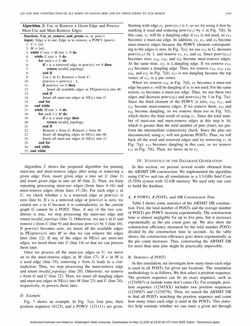
Algorithm 2: Use or Remove a Given Edge and ProcessMust-Use and Must-Remove Edges

function: Use_or_remove_and_prune (u, m, powv)input: Edge u to use, Edge m to remove, a POWV (powv).

1: U = {u};2: M = {m};3: while U.size + M.size > 0 do4: while U.size > 0 do5: for each e ∈ U do6: if e is a removed edge or powv(e) == 0 then7: return invalid_topology;8: end if9: Use e in G; Remove e from U;

10: powv(e) = powv(e) - 1;11: if powv(e) == 0 then12: Insert all available edges in PE(powv(e)) into M;13: end if14: Insert all must-use edges in NE(e) into U.15: end for16: end while17: while M.size > 0 do18: for each e ∈ M do19: if e is a used edge then20: return invalid_topology;21: end if22: Remove e from G; Remove e from M;23: Insert all dangling edges in NE(e) into M;24: Insert all must-use edges in NE(e) into U;25: end for26: end while27: end while

Algorithm 2 shows the proposed algorithm for pruningmust-use and must-remove edges after using or removing agiven edge. First, insert given edge u into set U (line 1)and insert given edge m into set M (line 2). Then, we keeprepeating processing must-use edges (from lines 4–16) andmust-remove edges (from lines 17–26). For each edge e inU, we check whether e is a removed edge or powv(e) iszero (line 6). If e is a removed edge or powv(e) is zero, wecannot use e in G because it is contradictory, so the currentgraph G cannot be a POST. Thus, if any of the two con-ditions is true, we stop processing the must-use edge andreturn invalid_topology (line 7). Otherwise, we use e in G andremove e from U (line 9) and decrease powv(e) by 1 (line 10).If powv(e) becomes zero, we insert all the available edgesin PE(powv(e)) into M so that we can remove the edgeslater (line 12). If any of the edges in NE(e) are must-useedges, we insert them into U (line 14) so that we can processthem later.

Once we process all the must-use edges in U, we moveon to the must-remove edges in M (line 17). If e in M isa used edge (line 19), removing e from G leads to a con-tradiction. Thus, we stop processing the must-remove edgeand return invalid_topology (line 20). Otherwise, we removee from G and U (line 22). Then, we insert all dangling edgesand must-use edges in NE(e) into M (line 23) and U (line 24),respectively, to process them later.

D. Example

Fig. 7 shows an example. In Fig. 7(a), four pins, theirposition sequence (4123), and a POWV (121111) are given.

Starting with edge e1, powv(e1) is 1, so we try using it first bymarking it used and reducing powv(e1) by 1 in Fig. 7(b). Inthis case, e1 will be a dangling edge if e13 is not used, so e13becomes a must-use edge. In addition, e2, e3, and e4 becomemust-remove edges because the POWV element correspond-ing to the edges is zero. In Fig. 7(c), we use e13 in G, decreasepowv(e13) by 1, and remove e2, e3, and e4. Since powv(e13)

becomes zero, e16, e19, and e22 become must-remove edges.At the same time, e15 is a dangling edge. If we remove e15,e14 becomes a dangling edge. Thus, we remove e14, e15, e16,e19, and e22 in Fig. 7(d). e13 is not dangling because the topvertex of e13 is a pin vertex.

When we remove e16 in Fig. 7(d), e5 becomes a must-useedge because e1 will be dangling if e5 is not used. For the samereason, e9 becomes a must-use edge. Thus, we use these twoedges and decrease powv(e5) and powv(e9) by 1 in Fig. 7(e).Since the third element of the POWV is zero, e10, e11, ande12 become must-remove edges. If we remove them, e23 ande24 become dangling, so we remove them too in Fig. 7(f),which shows the final result of using e1. Since the total num-ber of must-use and must-remove edges at this step is 16,which is greater than the total number of pins (four), we per-form the intermediate connectivity check. Since the pins aredisconnected, using e1 will not generate POSTs. Thus, we rollback all the used and removed edges and try removing e1 inFig. 7(g). e13 becomes dangling in this case, so we removee13 in Fig. 7(h). Then, we move on to e2.

IV. STATISTICS OF THE DATABASE GENERATION

In this section, we present several results obtained fromthe ARSMT DB construction. We implemented the algorithmusing C/C++ and ran all simulations in a 3.3-GHz Intel Corei5-3550 system with 32-GB memory. We used only one coreto build the database.

A. # POWVs, # POSTs, and DB Construction Time

Table I shows some statistics of the ARSMT DB construc-tion. First, the total number of POSTs and the average numberof POSTs per POWV increase exponentially. The constructiontime is almost negligible for up to five pins, but it increasesexponentially as the pin count goes up. We also show theconstruction efficiency measured by the total number POSTsdivided by the construction time in seconds. As the tableshows, the construction efficiency goes down exponentially asthe pin count increases. Thus, constructing the ARSMT DBfor more than nine pins might be practically impossible.

B. Statistics of POSTs

In this simulation, we investigate how many times each edgeis used in all POSTs for given pin locations. The simulationmethodology is as follows. We first select a position sequence.The position sequence can be an exact sequence, such as(1234567) or include some don’t-cares (X). For example, posi-tion sequence (12345XX) includes two position sequences(1234567) and (1234576). Then, we search the ARSMT DBto find all POSTs matching the position sequence and counthow many times each edge is used in the POSTs. This statis-tics help estimate whether we can route a given net through



(a) (b) (c) (d)

(e) (f) (g) (h)

Fig. 7. Example of edge pruning.

TABLE ISTATISTICS OF THE CONSTRUCTION OF ALL POSTS. “CON. TIME” IS THE CONSTRUCTION TIME FOR ALL THE POSTS FOR EACH PIN COUNT AND

“CON. EFF.” IS THE CONSTRUCTION EFFICIENCY MEASURED BY THE NUMBER OF TOTAL POSTS OVER THE CONSTRUCTION TIME (IN SECONDS)

(a) (b) (c) (d)

(e) (f) (g) (h)

Fig. 8. Statistics of POSTs for seven pins. The red edges are not used at all in any POSTs. Thicker edges are used in more POSTs than thinner edges. Greenrectangles are pins. Position sequences are as follows. (a) (1XXXXXX), (b) (X1XXXXX), (c) (XX1XXXX), (d) (XXX1XXX), (e) (X47X16X), (f) (3561724),(g) (2514736), which is a position sequence having the fewest POSTs, and (h) (1734652), which is a position sequence having the most POSTs. X is adon’t-care.

noncongested area. If an edge is used in most of the POSTsfor given pin locations, for example, it would be hard to routethe net without using the edge.

Fig. 8 shows eight examples for seven pins. In the figures,the thickness of a black edge is proportional to the number oftimes it is used. Red edges are not used at all. Green rectan-gles are pins. First, Fig. 8(a) shows the usage of the edges for(1XXXXXX), i.e., one of the pins is located at (0, 0). The two

edges adjacent to vertex (0, 0) are heavily used in the POSTsand the edges in the center area are also used in many POSTs.Thus, it would not be possible to route a net through the cen-ter area if the position sequence of the net is (1XXXXXX).Fig. 8(b) shows the edge usage for (X1XXXXX). In this case,none of the POSTs uses edges eh(0, 0), ev(0, 0), eh(0, 6),and ev(5, 0) no matter where the other six pins are located.Similarly, position sequences (XX1XXXX) and (XXX1XXX)



TABLE IIEFFECTIVENESS (RUNTIME IN SECONDS) OF THE PRUNING ALGORITHMS.

ALL: ENABLING ALL PRUNING ALGORITHMS. THE OTHER FOUR

COLUMNS ARE DISABLING: 1) ZERO POWV ELEMENTS; 2) MUST-USE

EDGES; 3) MUST-REMOVE EDGES; AND 4) INTERMEDIATE

CONNECTIVITY CHECK

do not use the same four edges and heavily use the right edgeof the pin vertex and the edges in the center of the grid asshown in Fig. 8(c) and (d). Fig. 8(e) shows the usage forposition sequence (X47X16X), which we picked randomly.For this position sequence, some edges, such as eh(1, 3),eh(4, 2), and ev(4, 5) around the middle of the grid are used inmany POSTs. Fig. 8(f) shows the usage of an exact positionsequence (3561724). Since the pins are distributed around theboundaries of the grid, the edges in the center area are used inmany POSTs. Fig. 8(g) shows the usage for (2514736), whichis a position sequence having the fewest POSTs and Fig. 8(h)shows the usage for (1734652), which is a position sequencehaving the most POSTs.

C. Effectiveness of the Pruning Algorithms

We use four pruning algorithms: 1) pruning by zero POWVelements; 2) pruning by must-use edges; 3) pruning by must-remove edges; and 4) intermediate connectivity check, toreduce the POST construction time. Thus, we measured theeffectiveness of each algorithm by disabling each of themwhile enabling all the other techniques. Table II shows thatpruning by must-use edges is the most effective technique.However, the other three pruning techniques also help reducethe runtime considerably.

D. POSTs Using/Not Using Specific Edges

A representative application of the proposed algorithmis generating multiple routing topologies for global rout-ing. Generating multiple RSMTs for each net can effectivelyreduce routing overflows, minimize routing congestion, andreduce the total coupling capacitance. In this section, we showhow to use the ARSMT DB to avoid nonpreferred (such ascongested) area and/or use preferred (such as noncongested)area. Suppose a set of pin locations and nonpreferred regionare given. Then, we search the ARSMT DB to find all POWVsbelonging to the position sequence of the pin locations andhaving the shortest wirelength. For each POST belonging tothe POWVs, we check whether the POST uses any edges inthe nonpreferred region. Finally, we return all the POSTs notusing any edges in the nonpreferred region. Fig. 9 shows anexample for position sequence (3561724) shown in Fig. 8(f).We searched for POSTs not containing the removed edgesin Fig. 9. The POST in the figure shows one of the POSTssatisfying the condition.

The search time consists of: 1) finding the positionsequence; 2) finding the set P all the POWVs belonging tothe position sequence and having the shortest wirelength; and3) checking whether each POST in P contains specific edges.

Fig. 9. POST not using specific edges for position sequence (3561724).

(a) (b) (c) (d)

Fig. 10. Four RSMTs for position sequence (3142). (a) and (b) for POWV121111 and (c) and (d) for POWV 111121.

The runtime of the first step is negligible and the complex-ity of the second step is approximately O(n · 2n), where n isthe number of pins. The exponential term comes from the totalnumber of POWVs belonging to a position sequence as shownin Table I and the multiplication factor n comes from the totalnumber of multiplications for the dot product computation.The complexity of the third step is approximately O(k · 3n),where n is the number of pins. The exponential term comesfrom the total number of POSTs for a POWV and k is thenumber of edges in the nonpreferred and/or preferred regions.

Notice that this does not solve the obstacle-avoiding RSMTconstruction problem that finds RSTs having the minimumwirelength for given pin locations and obstacles. Rather,we return all POSTs (or RSMTs if their POWVs have theminimum wirelength) that use and/or do not use specific edges.

E. Multiple RSTs for More Than Nine Pins

For high-degree nets having more than nine pins, it mightbe inefficient or impossible (due to the large database size)to build and use a POST database. However, the proposedalgorithm is not limited to constructing RSMTs. Rather, if pinlocations and a wirelength vector (WV) are given, the algo-rithm can construct all RSTs belonging to the given WV. Forhigh-degree nets, therefore, we can run FLUTE to constructan RST, obtain its WV, and run the proposed algorithm toobtain multiple RSTs. In this experiment, we tried construct-ing multiple RSTs using FLUTE for a few cases. Constructingall RSTs for a 10-pin, an 11-pin, and a 12-pin cases (each withone WV) found 324, 6390, and 870 RSTs in 10.9 s, 73.0 s,and 7.9 s, respectively. The 12-pin case had a smaller searchspace than the 10- and 11-pin cases, so it took only 7.9 s.

V. APPLICATIONS

In this section, we present two applications that can usethe ARSMT DB: 1) timing-driven RSMT construction and2) congestion-aware global routing.

A. Timing-Driven RSMT Construction

The sinks of a net generally have different timing con-straints. Thus, generating routing topologies that can minimize



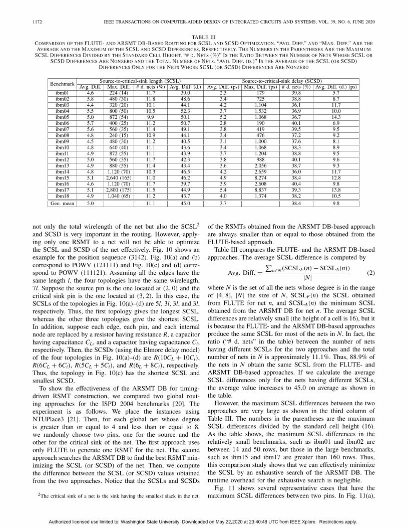
TABLE IIICOMPARISON OF THE FLUTE- AND ARSMT DB-BASED ROUTING FOR SCSL AND SCSD OPTIMIZATION. “AVG. DIFF.” AND “MAX. DIFF.” ARE THE

AVERAGE AND THE MAXIMUM OF THE SCSL AND SCSD DIFFERENCES, RESPECTIVELY. THE NUMBERS IN THE PARENTHESES ARE THE MAXIMUM

SCSL DIFFERENCES DIVIDED BY THE STANDARD CELL HEIGHT. “# D. NETS (%)” IS THE RATIO BETWEEN THE NUMBER OF NETS WHOSE SCSL OR

SCSD DIFFERENCES ARE NONZERO AND THE TOTAL NUMBER OF NETS. “AVG. DIFF. (D.)” IS THE AVERAGE OF THE SCSL (OR SCSD)DIFFERENCES ONLY FOR THE NETS WHOSE SCSL (OR SCSD) DIFFERENCES ARE NONZERO

not only the total wirelength of the net but also the SCSL2

and SCSD is very important in the routing. However, apply-ing only one RSMT to a net will not be able to optimizethe SCSL and SCSD of the net effectively. Fig. 10 shows anexample for the position sequence (3142). Fig. 10(a) and (b)correspond to POWV (121111) and Fig. 10(c) and (d) corre-spond to POWV (111121). Assuming all the edges have thesame length l, the four topologies have the same wirelength,7l. Suppose the source pin is the one located at (2, 0) and thecritical sink pin is the one located at (3, 2). In this case, theSCSLs of the topologies in Fig. 10(a)–(d) are 5l, 3l, 3l, and 3l,respectively. Thus, the first topology gives the longest SCSL,whereas the other three topologies give the shortest SCSL.In addition, suppose each edge, each pin, and each internalnode are replaced by a resistor having resistance R, a capacitorhaving capacitance CL, and a capacitor having capacitance Ci,respectively. Then, the SCSDs (using the Elmore delay model)of the four topologies in Fig. 10(a)–(d) are R(10CL + 10Ci),R(6CL + 6Ci), R(5CL + 5Ci), and R(6L + 8Ci), respectively.Thus, the topology in Fig. 10(c) has the shortest SCSL andsmallest SCSD.

To show the effectiveness of the ARSMT DB for timing-driven RSMT construction, we compared two global rout-ing approaches for the ISPD 2004 benchmarks [20]. Theexperiment is as follows. We place the instances usingNTUPlace3 [21]. Then, for each global net whose degreeis greater than or equal to 4 and less than or equal to 8,we randomly choose two pins, one for the source and theother for the critical sink of the net. The first approach usesonly FLUTE to generate one RSMT for the net. The secondapproach searches the ARSMT DB to find the best RSMT min-imizing the SCSL (or SCSD) of the net. Then, we computethe difference between the SCSL (or SCSD) values obtainedfrom the two approaches. Notice that the SCSLs and SCSDs

2The critical sink of a net is the sink having the smallest slack in the net.

of the RSMTs obtained from the ARSMT DB-based approachare always smaller than or equal to those obtained from theFLUTE-based approach.

Table III compares the FLUTE- and the ARSMT DB-basedapproaches. The average SCSL difference is computed by

Avg. Diff. =∑

n∈N(SCSLF(n) − SCSLA(n))

|N| (2)

where N is the set of all the nets whose degree is in the rangeof [4, 8], |N| the size of N, SCSLF(n) the SCSL obtainedfrom FLUTE for net n, and SCSLA(n) the minimum SCSLobtained from the ARSMT DB for net n. The average SCSLdifferences are relatively small (the height of a cell is 16), but itis because the FLUTE- and the ARSMT DB-based approachesproduce the same SCSL for most of the nets in N. In fact, theratio (“# d. nets” in the table) between the number of netshaving different SCSLs for the two approaches and the totalnumber of nets in N is approximately 11.1%. Thus, 88.9% ofthe nets in N obtain the same SCSL from the FLUTE- andARSMT DB-based approaches. If we calculate the averageSCSL differences only for the nets having different SCSLs,the average value increases to 45.0 on average as shown inthe table.

However, the maximum SCSL differences between the twoapproaches are very large as shown in the third column ofTable III. The numbers in the parentheses are the maximumSCSL differences divided by the standard cell height (16).As the table shows, the maximum SCSL differences in therelatively small benchmarks, such as ibm01 and ibm02 arebetween 14 and 50 rows, but those in the large benchmarks,such as ibm15 and ibm17 are greater than 160 rows. Thus,this comparison study shows that we can effectively minimizethe SCSL by an exhaustive search of the ARSMT DB. Theruntime overhead for the exhaustive search is negligible.

Fig. 11 shows several representative cases that have themaximum SCSL differences between two pins. In Fig. 11(a),



(a) (b)

(c)

(d)

(e)

Fig. 11. Two RSMTs having the maximum SCSL difference between two redpins for each position sequence. (a) Four-pin net. (b) Five-pin net. (c) Six-pinnet. (d) Seven-pin net. (e) Eight-pin net.

for example, the lengths between the two red pins are 2 and 4on the left- and right-hand sides, respectively, so the differenceis 2. Similarly, the differences in Fig. 11(b)–(e) are 2, 4, 6,and 10, respectively. Thus, the ARSMT DB could help timing-driven global routers find one or multiple RSMTs minimizingthe SCSL for a given net.

Table III also compares the FLUTE- and the ARSMT DB-based approaches for SCSD optimization. We used the Elmoredelay model to calculate the delay values. The output resis-tance of a driver is 100 �, the unit wire resistance andcapacitance are 2 � per length and 0.4 fF per length, respec-tively, and the capacitance of each pin is 5 fF. The averageSCSD difference between the two approaches is 3.7 ps, whichis almost negligible. In addition, the average SCSD differ-ence for the nets having difference SCSDs is only 9.8%.However, the maximum SCSD differences are very large. Forexample, the maximum SCSD differences in the ibm15 andibm17 benchmarks are greater than 8 ns. Overall, the ARSMTDB can help find RSMTs having the minimum SCSD effi-ciently. Notice that buffer insertion along the RSMTs willreduce the SCSD differences between the two approaches,but the ARSMT DB can still help find minimum-SCSL andminimum-SCSD RSMTs.

B. Congestion-Aware Global Routing

Another representative application of the ARSMT DB isthe congestion-aware (routability-driven) global routing. Manyglobal routing algorithms use RSMTs to find high-quality rout-ing topologies [13]–[19]. However, all the RSMT generators

Fig. 12. Example for congestion cost computation.

generate only one RSMT for a net, which could result inserious routing congestion. In this experiment, we performglobal routing using the ARSMT DB to reduce the congestionwithout wirelength overhead.

The experiment is as follows. First, we place instances usingNTUPlace3 [21] and build a global routing data structure (bins,edges, etc.). Then, for each global net, we generate a routingtopology using FLUTE and proceed to the next net in theFLUTE-based global routing. In the ARSMT DB-based globalrouting, we obtain all RSMTs for each global net, compute thecongestion cost for each RSMT, and obtain the best RSMT thathas the lowest cost. We use the amount of overflows for thecongestion cost, which is defined as follows:

gi =∑

e∈Ei

(de − ce)u[de − ce] (3)

where gi is the congestion cost of net i, Ei the set of all theglobal routing edges that net i goes through, de the numberof nets going through e, ce the maximum capacity of e, andu[x] is the unit-step function. Fig. 12 shows an example fora two-pin net. The maximum capacity of each edge in thegrid is 5. The numbers in the figure show the numbers of netsgoing through the global routing edges. The congestion costfor topology A is (5+1−5)+(5+1−5)+0+0 = 2, whereasthat for topology B is (6+1−5)+(6+1−5)+0+0 = 4, so wechoose topology A to minimize the total overflow. For high-degree nets, we use FLUTE to get an RST for both FLUTE-and ARSMT DB-based global routing.

Table IV shows the global routing result for the ISPD 2004,2005, and 2006 benchmark suites [22], [23]. “# g. nets” is thenumber of global nets. Since we use the ARSMT DB only forlow-degree nets, the number of nets routed using the ARSMTDB (“# r. nets” in the table) is slightly less than the totalnumber of global nets. However, most of the global nets arelow-degree nets, so they can show the effectiveness of theARSMT DB. Notice that they have the same total wirelengthbecause both of them use RSMTs for low-degree nets and thesame RSTs for high-degree nets.

The table shows that the FLUTE-based routing has muchmore overflows than the ARSMT DB-based routing. On aver-age, the ARSMT DB-based routing has 85.39% less overflowsthan the FLUTE-based routing. In addition, the maximumoverflow of the ARSMT DB-based routing is less than thatof the FLUTE-based routing for all the benchmarks exceptadaptec5. On average, the ARSMT DB-based routing has83.71% lower maximum overflow than the FLUTE-based rout-ing. The average overflow (the total overflow over the numberof edges) of the ARSMT DB-based routing is 83.89% lessthan that of the FLUTE-based routing. Overall, the ARSMTDB-based sequential global routing optimizes the total over-flow, the number of overflow edges, the maximum overflow,



TABLE IVSEQUENTIAL GLOBAL ROUTING RESULT. “# G. NETS” IS THE TOTAL NUMBER OF GLOBAL NETS. “# R. NETS” IS THE NUMBER OF GLOBAL NETS

ROUTED USING THE ARSMT DB. “# OV” IS THE TOTAL NUMBER OF OVERFLOWS. “(F)” AND “(O)” ARE THE FLUTE- AND THE ARSMT DB-BASED

ROUTING, RESPECTIVELY. “% OV IMP.” IS (# OV(O) - # OV(F)) * 100/# OV(F). “M. OV” IS THE MAXIMUM OVERFLOW.“A. OV” IS THE AVERAGE

OVERFLOW. “RT” IS THE RUNTIME (IN SECONDS) FOR GLOBAL ROUTING. GM: GEOMETRIC MEAN. AM: ARITHMETIC MEAN

and the average overflow much more effectively than theFLUTE-based sequential global routing.

The runtime of the FLUTE-based routing is less than twoseconds for all the cases, whereas the runtime of the ARSMTDB-based routing is less than 30 s. The runtime ratio betweenthe ARSMT DB- and FLUTE-based routing is 21.76 on aver-age. However, the absolute runtime overhead is negligible asthe table shows.

VI. DATABASE SIZE REDUCTION

As shown in Section IV, the database size is prohibitivelylarge, especially when the pin count is nine. In this section,therefore, we present several techniques to reduce the size ofthe ARSMT DB, database loading time, and memory usage.

A. Raw Database

The raw ARSMT DB uses the database structure shown inFig. 13 to store the POST data. The database consists of posi-tion sequence lines, POWV lines, and POST lines. A positionsequence line is “P seq,” where “P” denotes a new posi-tion sequence and seq is its actual position sequence. All thePOWVs belonging to the position sequence appear betweenthe position sequence line and the next position sequence lineor the end of file. A POWV line is “V vec,” where “V” denotes

a new POWV and vec is its actual POWV. All the POSTsbelonging to the POWV appear between the POWV line andthe next POWV line or the next position sequence line orthe end of file. A POST line is “Hh_edgesVv_edges,” whereh_edges and v_edges are the coordinates of the horizontal andvertical edges, respectively.

h_edges consists of uppercase and lowercase alphabets,which are their x- and y-coordinates, respectively. The map-ping between an alphabet and its coordinate is that “A” or“a” corresponds to 0, “B” or “b” corresponds to 1, and theother alphabets are mapped into integers in a similar way. Forexample, “Ab” for a horizontal edge means eh(0, 1). To reducethe number of characters, horizontal edges having the same x-coordinate share the x-coordinate. Thus, “Abde” for horizontaledges denote three edges eh(0, 1), eh(0, 3), and eh(0, 4). Weprocess v_edges in the same way. The database size shown inthe 12th column (raw data table size) in Table I is the size ofthe database of the raw data.

B. Congruence and Difference Encoding

The input to the database generator is the raw databaseexplained in Fig. 13 and the output is an encoded database.Users can open the database, decode the data, and load it intotheir applications and use the raw data.



Fig. 13. Raw database structure and the proposed encoding and decodingflow for database size reduction.

Two techniques are used in [2] to reduce the database size ofFLUTE. The first technique is to use congruence. For exam-ple, position sequences (12345) and (54321) have the sameset of POSTs, but the POSTs are symmetric about the y-axis.Thus, we need to store POSTs only for one of them (calleda base position sequence). For the other position sequence,we can obtain all POSTs using a transformation rule betweenthe position sequences. In Fig. 13, therefore, only one line “P54321 P 12345 Y” suffices for storing all POSTs for posi-tion sequence (54321), where “Y” denotes the transformationrule (reflection over the y-axis). A congruence check betweentwo position sequences includes rotation of one of the positionsequences and the image of its reflection about the y-axis by90◦, 180◦, and 270◦.

The second technique used in [2] for database size reductionis to store only differences between two POSTs. As explainedin [2], many POSTs are similar to each other. Thus, FLUTEstores full data for a few POSTs and difference data for all theother POSTs. We apply a similar technique to the ARSMT DBas follows. Suppose we encode the (i + 1)th POST by compar-ing it with the ith POST. The format of the encoded POST isstill “Hh_edgesVv_edges.” If the (i+1)th POST has exactly thesame horizontal or vertical edges as the ith POST in column kor row k, we skip them. Otherwise, we store the column or rowcoordinate and the y- or x-coordinates of the edges used in thecolumn or row, respectively. For example, the raw data of thePOST in Fig. 14(a) is “HAaBbCbdDdVAbBdCdDe” and thatof the POST in Fig. 14(b) is “HAaBbCbdDeVAbBdCdDd.”If we store only the differences, however, the latter becomes“HDeVDd.”

C. Simulation Results

Table V shows statistics of database encoding and databaseloading time. We used a 7200-RPM hard disk drive for thesimulation. The sizes of the raw and encoded database are thesame as the table sizes shown in Table I. As the table shows,

(a) (b)

Fig. 14. Difference encoding. (a) HAaBbCbdDdVAbBdCdDe. (b) HDeVDdrelative to (a). The coordinate systems in (a) and (b) are for the horizontaland vertical edges, respectively.

TABLE VSTATISTICS OF DATABASE ENCODING AND DATABASE LOADING TIME

(FROM A 7200-RPM HDD). “R (C)” AND “R (D)” ARE THE DATABASE

SIZE REDUCTION RATIOS BY THE CONGRUENCE CHECK AND THE

DIFFERENCE ENCODING, RESPECTIVELY. THE LOADING TIME

INCLUDES THE RUNTIME FOR DIFFERENCE DECODING. MEMORY

USAGE IS THE SIZE OF THE MEMORY ALLOCATED TO

STORE THE POST DATABASE IN MEMORY

the size of the encoded database is much less than that ofthe raw database. The database size reduction ratio (# gener-ated POSTs divided by the total # POSTs) by the congruencecheck is approximately 0.375 and 0.128 for the three- andnine-pin cases, respectively, and varies between the two valuesfor the four- to eight-pin cases as shown in Table V. In thebest case, eight position sequences are congruent for whichthe database size reduction ratio is 0.125. As the pin countincreases, more position sequences are congruent to each other,so the database size reduction ratio approaches 0.125. Thedatabase size reduction ratio by the difference encoding variesbetween 0.29 and 0.88. Thus, both the congruence-based anddifference-encoding-based database size reduction techniquesare very effective.

Table V also shows database loading time and memoryusage, which is the “Load” process in Fig. 13. The loadingtime is almost negligible for all the cases. Although the loadingtime for the nine-pin case is approximately ten minutes, globalrouting of large designs generally takes much longer time thanthat [24], [25]. The maximum memory usage is 20 GB, whichis also acceptable for the design of large, complex layouts.Notice that the loaded database is still difference-encoded.Thus, processing a database query requires real-time con-gruence check and difference decoding. However, the actualruntime of the congruence check and difference decoding isnegligible .

VII. CONCLUSION

In this paper, we proposed an efficient algorithm to createa database for an efficient RSMT construction. The ARSMTDB can return all the RSMTs for a given set of pins in no



time, so its application is numerous. We showed two repre-sentative applications: 1) SCSL and 2) SCSD minimizationand congestion-aware global routing. Use of the ARSMT DBhelps minimize the SCSL and SCSD for a given net and alsominimize routing congestion during global routing effectively.Since the size of the ARSMT DB is large, we proposed tech-niques to reduce the size of the ARSMT DB. We believe thatthe ARSMT DB can help all the electronic design automationsoftware improve the quality of layouts and reduce the runtimefor placement, routing, and various optimization.

REFERENCES

[1] GeoSteiner. Software for Computing Steiner Trees. Accessed: Jan. 2017.[Online]. Available: http://www.geosteiner.com

[2] C. Chu and Y.-C. Wong, “FLUTE: Fast lookup table based rectilin-ear Steiner minimal tree algorithm for VLSI design,” IEEE Trans.Comput.-Aided Design Integr. Circuits Syst., vol. 27, no. 1, pp. 70–83,Jan. 2008.

[3] M. Hanan, “On Steiner’s problem with rectilinear distance,” SIAM J.Appl. Math., vol. 14, no. 2, pp. 255–265, Mar. 1966.

[4] J. L. Ganley and J. P. Cohoon, “Optimal rectilinear Steiner minimaltrees in O(n22.62n) time,” in Proc. Can. Conf. Comput. Geometry, 1994,pp. 308–313.

[5] J. L. Ganley and J. P. Cohoon, “A faster dynamic programming algo-rithm for exact rectilinear Steiner minimal trees,” in Proc. Great LakesSymp. VLSI, 1994, pp. 238–241.

[6] J. L. Ganley and J. P. Cohoon, “Improved computation of optimal rec-tilinear Steiner minimal trees,” Int. J. Comput. Geometry Appl., vol. 7,no. 5, pp. 457–472, Oct. 1997.

[7] M. R. Garey and D. S. Johnson, Computers and Intractability: A Guideto the Theory of NP-Completeness. New York, NY, USA: Freeman,1979.

[8] J. Griffith, G. Robins, J. S. Salowe, and T. Zhang, “Closing the gap:Near-optimal Steiner trees in polynomial time,” IEEE Trans. Comput.-Aided Design Integr. Circuits Syst., vol. 13, no. 11, pp. 1351–1365,Nov. 1994.

[9] M. Borah, R. M. Owens, and M. J. Irwin, “An edge-based heuristicfor Steiner routing,” IEEE Trans. Comput.-Aided Design Integr. CircuitsSyst., vol. 13, no. 12, pp. 1563–1568, Dec. 1994.

[10] I. I. Mandoiu, V. V. Vazirani, and J. L. Ganley, “A new heuristic for recti-linear Steiner trees,” IEEE Trans. Comput.-Aided Design Integr. CircuitsSyst., vol. 19, no. 10, pp. 1129–1139, Oct. 2000.

[11] A. B. Kahng, I. I. Mandoiu, and A. Z. Zelikovsky, “Highly scalablealgorithms for rectilinear and octilinear Steiner trees,” in Proc. AsiaSouth Pac. Design Autom. Conf., Jan. 2003, pp. 827–833.

[12] H. Zhou, “Efficient Steiner tree construction based on spanning graphs,”IEEE Trans. Comput.-Aided Design Integr. Circuits Syst., vol. 23, no. 5,pp. 704–710, May 2004.

[13] M. Cho and D. Z. Pan, “BoxRouter: A new global router based on boxexpansion and progressive ILP,” IEEE Trans. Comput.-Aided DesignIntegr. Circuits Syst., vol. 26, no. 12, pp. 2130–2143, Dec. 2007.

[14] Z. Cao, T. Jing, J. Xiong, Y. Hu, L. He, and X. Hong, “DpRouter: A fastand accurate dynamic-pattern-based global routing algorithm,” in Proc.Asia South Pac. Design Autom. Conf., 2007, pp. 256–261.

[15] M. M. Ozdal and M. D. F. Wong, “Archer: A history-driven global rout-ing algorithm,” in Proc. IEEE Int. Conf. Comput.-Aided Design, 2007,pp. 488–495.

[16] M. D. Moffitt, “MaizeRouter: Engineering an effective global router,”IEEE Trans. Comput.-Aided Design Integr. Circuits Syst., vol. 27, no. 11,pp. 2017–2026, Nov. 2008.

[17] Y. Xu, Y. Zhang, and C. Chu, “FastRoute 4.0: Global router with efficientvia minimization,” in Proc. Asia South Pac. Design Autom. Conf., 2009,pp. 576–581.

[18] T.-H. Wu, A. Davoodi, and J. T. Linderoth, “GRIP: Scalable 3D globalrouting using integer programming,” in Proc. ACM Design Autom. Conf.,2009, pp. 320–325.

[19] Y.-J. Chang, Y.-T. Lee, J.-R. Giao, P.-C. Wu, and T.-C. Wang,“NTHU-Route 2.0: A robust global router for modern designs,” IEEETrans. Comput.-Aided Design Integr. Circuits Syst., vol. 29, no. 12,pp. 1931–1944, Dec. 2010.

[20] N. Viswanathan and C. C.-N. Chu, “FastPlace: Efficient analytical place-ment using cell shifting, iterative local refinement and a hybrid netmodel,” in Proc. Int. Symp. Phys. Design, Mar. 2004, pp. 26–33.

[21] T.-C. Chen, Z.-W. Jiang, T.-C. Hsu, H.-C. Chen, and Y.-W. Chang,“NTUplace3: An analytical placer for large-scale mixed-size designswith preplaced blocks and density constraints,” IEEE Trans. Comput.-Aided Design Integr. Circuits Syst., vol. 27, no. 7, pp. 1228–1240,Jul. 2008.

[22] G.-J. Nam, C. J. Alpert, P. Villarrubia, B. Winter, and M. Yildiz, “TheISPD2005 placement contest and benchmark suite,” in Proc. Int. Symp.Phys. Design, 2005, pp. 216–220.

[23] G.-J. Nam, “The ISPD 2006 placement contest: Benchmark suite andresults,” in Proc. Int. Symp. Phys. Design, 2006, p. 167.

[24] T.-H. Wu, A. Davoodi, and J. T. Linderoth, “GRIP: Global routingvia integer programming,” IEEE Trans. Comput.-Aided Design Integr.Circuits Syst., vol. 30, no. 1, pp. 72–84, Jan. 2011.

[25] K.-R. Dai, W.-H. Liu, and Y.-L. Li, “NCTU-GR: Efficient simulatedevolution-based rerouting and congestion-relaxed layer assignment on3-D global routing,” IEEE Trans. Comput.-Aided Design Integr. CircuitsSyst., vol. 20, no. 3, pp. 459–472, Mar. 2012.

Sheng-En David Lin (S’16) received the B.S.degree in electrical engineering from WashingtonState University, Pullman, WA, USA, in 2014, wherehe is currently pursuing the Ph.D. degree with theDepartment of Electrical Engineering and ComputerScience.

His current research interests include modelingfor very large scale integration (VLSI) circuits andsystems and algorithms for VLSI CAD automa-tion with current focus on designing of monolithic3-D ICs.

Dae Hyun Kim (S’08–M’12) received the B.S.degree in electrical engineering from Seoul NationalUniversity, Seoul, South Korea, in 2002, and theM.S. and Ph.D. degrees in electrical and com-puter engineering from the Georgia Institute ofTechnology, Atlanta, GA, USA, in 2007 and 2012,respectively.

He is an Assistant Professor with the Schoolof Electrical Engineering and Computer Science,Washington State University, Pullman, WA, USA.He researched on physical layout optimization with

Cadence Design Systems, Inc., San Jose, CA, USA, from 2012 to 2014. Hiscurrent research interests include electronic design automation and computer-aided design for very large scale integration (VLSI), high-performance and/orlow-power VLSI and computer systems, and 3-D integrated circuits andsystems.

Dr. Kim was a recipient of the Defense Advanced Research Projects AgencyYoung Faculty Award in 2016.


construction of all rectilinear steiner minimum trees on...

Documents