construction air quality conformity assessment · pdf fileconstruction air quality conformity...
TRANSCRIPT

ACOUSTICS – VIBRATION – AIR & WATER QUALITY – FORENSIC ENGINEERING EXPERT WITNESS – ENVIRONMENTAL ASSESSMENTS AND COMPLIANCE
CONSTRUCTION AIR QUALITY CONFORMITY ASSESSMENT
TULE WIND PROJECTBOULEVARD, CA
Submitted to:
Mr. Patrick O'NeillHDR
8690 Balboa Avenue, Suite 200San Diego, CA 92123
Investigative Science and Engineering, Inc. Scientific, Environmental, and Forensic Consultants
P.O. Box 488 / 1134 D StreetRamona, CA 92065
(760) 787-0016www.ise.us
ISE Project #10-001
September 14, 2010 (Revised)

© 2010 Investigative Science and Engineering, Inc. The leader in Scientific Consulting and Research…
REPORT CONTENTS
INTRODUCTION AND DEFINITIONS 1
Existing Site Characterization 1Project Description 1Air Quality Definitions 12
THRESHOLDS OF SIGNIFICANCE 14National Environmental Policy Act (NEPA) Thresholds 14California Environmental Quality Act (CEQA) Thresholds 17CEQA Air Quality Screening Standards 17SDAPCD Criteria Pollutant Standards 17Combustion Toxics Risk Factors 20
ANALYSIS METHODOLOGY 21Ambient Air Quality Data Collection 22Construction Air Quality Modeling 25Aggregate Vehicle Emission Air Quality Modeling 28Vehicular CO / NOx / PM10 / PM2.5 Conformity Assessment 30
FINDINGS 31Existing Climate Conditions 31Existing Air Quality Levels 33Project Construction Emission Findings 42Odor Impact Potential from Proposed Site 48Construction Worker Vehicular Emission Levels 49Predicted CO / NOx / PM10 / PM2.5 Concentration Levels 49
CONCLUSIONS AND RECOMMENDATIONS 52Aggregate Project Emissions 52Consistency with Regional Air Quality Management Plans 52
CERTIFICATION OF ACCURACY AND QUALIFICATIONS 53APPENDICES / SUPPLEMENTAL INFORMATION 54
EMFAC 2007 EMISSION FACTOR TABULATIONS – SCENARIO YEAR 2012 54SCREEN3 Model Output for Criteria Pollutants: CO, NOx, SOx, and PM10 56CALINE4 SOLUTION SPACE RESULTS – SCENARIO CO 64CALINE4 SOLUTION SPACE RESULTS – SCENARIO NOX 65CALINE4 SOLUTION SPACE RESULTS – SCENARIO PM10 66
INDEX OF IMPORTANT TERMS 67

© 2010 Investigative Science and Engineering, Inc. The leader in Scientific Consulting and Research…
LIST OF TABLES
TABLE 1: Thresholds of Significance for Air Quality Impacts 18TABLE 2: Baseline ‘Tier 0’ AP-42 Equipment Pollutant Generation Rates 26TABLE 3a: Alpine Monitoring Station – Maximum Hourly O3 Levels 33TABLE 3b: Alpine Monitoring Station – Maximum Eight-Hour O3 Levels 34TABLE 3c: Alpine Monitoring Station – Maximum Daily PM2.5 Levels 35TABLE 3d: Alpine Monitoring Station – Maximum Hourly NO2 Levels 36TABLE 3e: El Centro Monitoring Station – Maximum Hourly O3 Levels 36TABLE 3f: El Centro Monitoring Station – Maximum Eight-Hour O3 Levels 37TABLE 3g: El Centro Monitoring Station – Maximum Daily PM2.5 Levels 38TABLE 3h: El Centro Monitoring Station – Maximum Daily PM10 Levels 39TABLE 3i: El Centro Monitoring Station – Maximum Eight-Hour CO Levels 40TABLE 3j: El Centro Monitoring Station – Maximum Hourly NO2 Levels 40TABLE 4: Ambient Air Quality Monitoring Results 41TABLE 5a: Predicted Construction Emissions – Rough Grading / Tower Base Work 42TABLE 5b: Predicted Construction Emissions – Underground Construction / Tower Work 43TABLE 6: Predicted Onsite Diesel-Fired Construction Emission Rates (Tier 0) 47TABLE 7: SCREEN3 Predicted Diesel-Fired Emission Concentrations 47TABLE 8: Construction Worker Trip Emissions – Tule Wind Project 50TABLE 9: Roadway Segment Incremental Project Increases for CO, NOX, PM10 and PM2.5 51TABLE 10: Aggregate Construction Emissions Synopsis – Tule Wind Project 52

© 2010 Investigative Science and Engineering, Inc. The leader in Scientific Consulting and Research…
LIST OF FIGURES / MAPS / ADDENDA
FIGURE 1a: Project Area Vicinity Map 2 FIGURE 1b: Project Jurisdictional Land Use Map 3 FIGURE 2a: Proposed Tule Wind Project Overview Map 4 FIGURE 2b: Proposed Tule Wind Project Turbine Configuration – Sheet 1 5 FIGURE 2c: Proposed Tule Wind Project Turbine Configuration – Sheet 2 6 FIGURE 2d: Proposed Tule Wind Project Turbine Configuration – Sheet 3 7 FIGURE 2e: Proposed Tule Wind Project Turbine Configuration – Sheet 4 8 FIGURE 3: Proposed Tule Wind Project Access Road Configuration 9 FIGURE 4: Isometric Aerial Photograph w/ Proposed Project Uses 11FIGURE 5: Ambient Air Quality Standards Matrix 15FIGURE 6: Ambient Air Quality Monitoring Station Location Map 23FIGURE 7a and -b: Ambient Air Quality Sampling Location AQ 1 / Analysis Procedure 24FIGURE 8: Project Air Basin Aerial Map 32FIGURE 9: Spectral Content of Ambient Air Monitoring Location AQ1 41FIGURE 10: Predicted Combustion-Fired Diesel PM10 Dispersion Pattern 48


© 2010 Investigative Science and Engineering, Inc. The leader in Scientific Consulting and Research…
INTRODUCTION AND DEFINITIONS
Existing Site Characterization
The project site has an effective working footprint of 38.3 square-miles (24,500acres)1 located in the eastern portion of San Diego County in the community of Boulevard, CA as shown in Figure 1a on the following page. Regional access to the site is obtained from the Ribbonwood Road exit, off Interstate 8 (I-8) and McCain Valley Road.
The development site consists of steep and rugged terrain areas located primarily on federal lands managed by the Bureau of Land Management (BLM), or other public lands, such as those maintained by the California State Lands Commission, and the Cuyapaipe Band of Mission Indians (denoted as the red shaded areas, as shown in Figure 1b on Page 3 of this report). A small portion of the project site resides on privately owned lands under the jurisdiction of the County of San Diego, with the majority of the project area being outside the land use jurisdiction of the County of San Diego. Elevations across the site are markedly varied and range from approximately 3,500 to 5,600 feet above mean sea level (MSL).
Project Description
The Tule Wind Project proposes the construction of a 200-megawatt (MW) windturbine power generating facility within the McCain Valley area of eastern San Diego County. Pacific Wind Development LLC is proposing to construct and operate the Tule Wind Project located near Boulevard, California. The proposed wind generation project will consist of the following components:
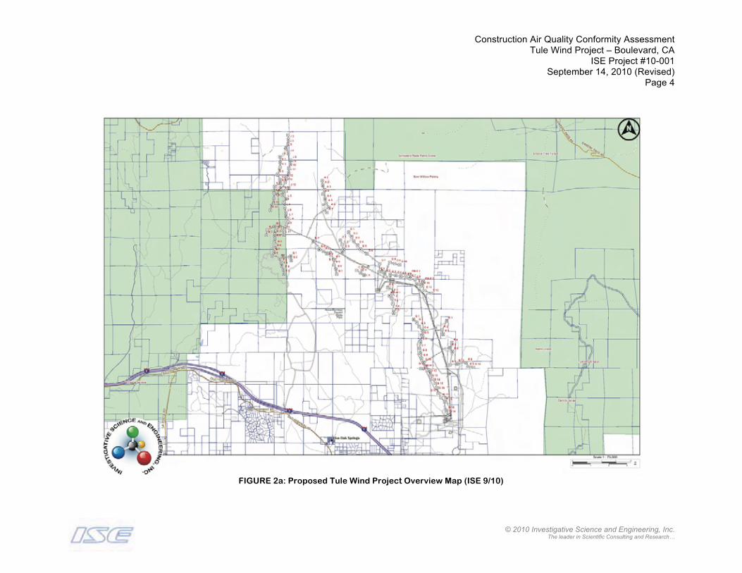
• Up to 134 wind turbines, ranging in size between 328 and 492 feet in height, to produce 200 MW of electricity, as denoted in Figures 2a through -e starting on Page 4 of this report;
• Construct a five-acre collector substation and five-acre operation and maintenance (O&M) facility as denoted as brown polygons in Figures 2a through -e;
• Construct a 34.5 kV electrical collector grid (denoted as –E– in Figures 2a through -e) connecting the turbines to the collector substation, and construct a 138-kilovolt (kV) overhead and underground transmission line (denoted as –T– in Figures 2a through -e) running south from the proposed substation to the San Diego Gas & Electric (SDG&E) Boulevard Substation;
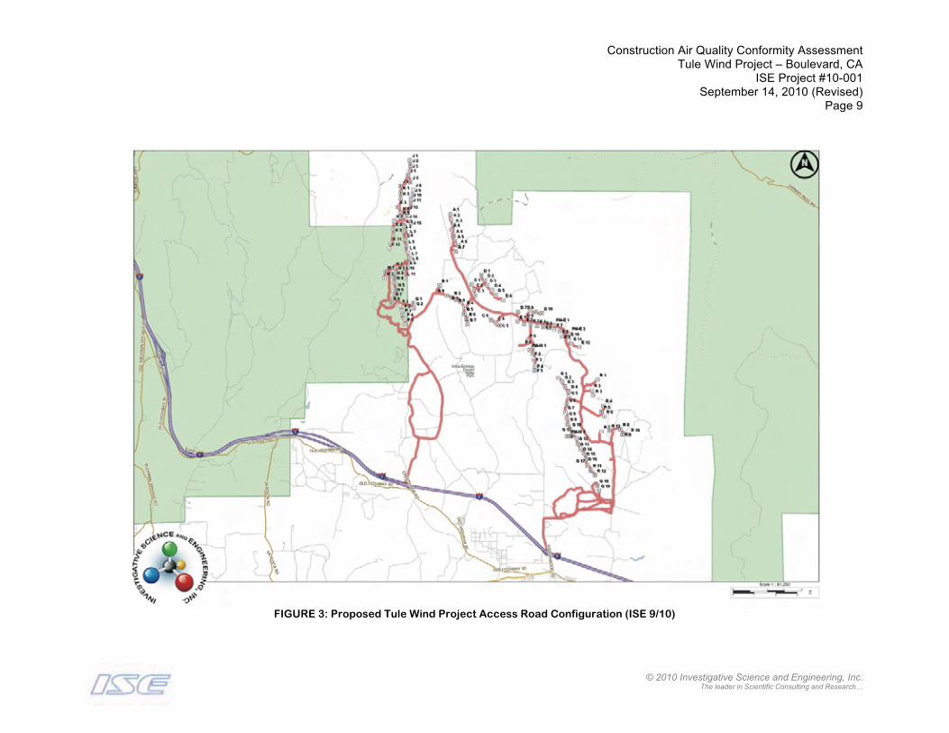
• Construct access roads between turbines and perform improvements to existing roadways, as denoted in red in Figure 3 on Page 9 of this report;
• Construct a temporary five-acre batch plant for construction activities, as well as a temporary 10-acre parking area, and nineteen two-acre lay down areas; and,
• Construct two permanent meteorological towers and one SODAR Unit. 1 Determined to consist of the worst-case polygon enclosing the turbine locations and access roads shown in Figure 3 of this report.

Construction Air Quality Conformity AssessmentTule Wind Project – Boulevard, CA
ISE Project #10-001September 14, 2010 (Revised)
Page 2
© 2010 Investigative Science and Engineering, Inc. The leader in Scientific Consulting and Research…
FIGURE 1a: Project Area Vicinity Map (ISE 9/10)

Construction Air Quality Conformity AssessmentTule Wind Project – Boulevard, CA
ISE Project #10-001September 14, 2010 (Revised)
Page 3
© 2010 Investigative Science and Engineering, Inc. The leader in Scientific Consulting and Research…
FIGURE 1b: Project Jurisdictional Land Use Map (ISE 9/10)
Construction Air Quality Conformity AssessmentTule Wind Project – Boulevard, CA
ISE Project #10-001September 14, 2010 (Revised)
Page 4
© 2010 Investigative Science and Engineering, Inc. The leader in Scientific Consulting and Research…
FIGURE 2a: Proposed Tule Wind Project Overview Map (ISE 9/10)

Construction Air Quality Conformity AssessmentTule Wind Project – Boulevard, CA
ISE Project #10-001September 14, 2010 (Revised)
Page 5
© 2010 Investigative Science and Engineering, Inc. The leader in Scientific Consulting and Research…
FIGURE 2b: Proposed Tule Wind Project Turbine Configuration – Sheet 1 (ISE 9/10)

Construction Air Quality Conformity AssessmentTule Wind Project – Boulevard, CA
ISE Project #10-001September 14, 2010 (Revised)
Page 6
© 2010 Investigative Science and Engineering, Inc. The leader in Scientific Consulting and Research…
FIGURE 2c: Proposed Tule Wind Project Turbine Configuration – Sheet 2 (ISE 9/10)

Construction Air Quality Conformity AssessmentTule Wind Project – Boulevard, CA
ISE Project #10-001September 14, 2010 (Revised)
Page 7
© 2010 Investigative Science and Engineering, Inc. The leader in Scientific Consulting and Research…
FIGURE 2d: Proposed Tule Wind Project Turbine Configuration – Sheet 3 (ISE 9/10)

Construction Air Quality Conformity AssessmentTule Wind Project – Boulevard, CA
ISE Project #10-001September 14, 2010 (Revised)
Page 8
© 2010 Investigative Science and Engineering, Inc. The leader in Scientific Consulting and Research…
FIGURE 2e: Proposed Tule Wind Project Turbine Configuration – Sheet 4 (ISE 9/10)
Construction Air Quality Conformity AssessmentTule Wind Project – Boulevard, CA
ISE Project #10-001September 14, 2010 (Revised)
Page 9
© 2010 Investigative Science and Engineering, Inc. The leader in Scientific Consulting and Research…
FIGURE 3: Proposed Tule Wind Project Access Road Configuration (ISE 9/10)

Construction Air Quality Conformity AssessmentTule Wind Project – Boulevard, CA
ISE Project #10-001September 14, 2010 (Revised)
Page 10
© 2010 Investigative Science and Engineering, Inc. The leader in Scientific Consulting and Research…
Project construction activities will avoid excessive grading on roads, road embankments, ditches, and drainages to the extent possible to maintain a minimal footprint. A temporary construction work area will be cleared for each wind turbine tower. Work areas may vary in size, and may be constructed differently in keeping with each site’s topography (although for the purposes of analysis within this report, an average estimate of construction effort will be examined). The proposed construction influencearea (and subsequent study area within this report) is shown in Figure 4 on the following page.
Each turbine work area will require up to a 200-foot radius to be cleared and leveled. The cleared area is necessary for foundation excavation and construction, assembling turbine sections, and also to stage the construction crane, which will hoist turbine sections into place. The turbine construction area will not be paved. Permanent wind tower foundations will be approximately 60 feet in diameter, and seven to ten feet in depth. After turbine erection has been completed, a 9 to 10-foot wide area around the base of the tower will be surfaced with gravel. The gravel will provide a stable surface area for maintenance vehicles, and will minimize surface erosion and runoff.
Underground electrical and communications cables will be placed in a 3 to 5-foot wide, and 3 to 5-foot deep trench, generally along the length of the proposed turbine access roads. Electrical cables will be installed first and the trench will be partially backfilled before placing communications cables. The topsoil in the trench will be stripped and set aside before the trench is backfilled, with topsoil replaced on the uppermost layer. Concrete or fiberglass vaults and splice boxes will be placed at necessary locations. Boxes will have locked lids to prevent public access. The vaults will be about 5 x 5 x 8 feet, and will be placed approximately 2,500 feet apart.
Aboveground collector lines will use steel poles that are 60 to 80 feet in height; taller heights may be needed to cross washes or drainages. Aboveground lines are normally used to span canyons or streams to eliminate the habitat disturbance that trenching causes in these areas. The interconnection transmission line, operating at a voltage of 138 kV, and leading from the Project substation to the Boulevard substation will be above ground for all or a portion of its length. The exact location for transmission poles will be determined closer to final engineering and design.
Finally, roads will be designed in accordance with County Standards. Transportation routing will be conducted to minimize impacts to normal traffic flow during the transport of turbine components, main assembly cranes, and other large pieces of equipment. After construction is complete, the applicant will work to restore vegetation to pre-construction standards for all disturbed areas.

Construction Air Quality Conformity AssessmentTule Wind Project – Boulevard, CA
ISE Project #10-001September 14, 2010 (Revised)
Page 11
© 2010 Investigative Science and Engineering, Inc. The leader in Scientific Consulting and Research…
FIGURE 4: Isometric Aerial Photograph w/ Proposed Project Uses (ISE 9/10)

Construction Air Quality Conformity AssessmentTule Wind Project – Boulevard, CA
ISE Project #10-001September 14, 2010 (Revised)
Page 12
© 2010 Investigative Science and Engineering, Inc. The leader in Scientific Consulting and Research…
Upon completion of construction, the project would be supported by up to 10
permanent full-time or part-time employees on the Operations and Maintenance (O&M) staff. Typically, these staff will be present on site during normal business hours.Maintenance activities will be limited to areas accessible by the permanent access roadsprovided during the construction phase. Each turbine would be serviced approximately twice a year. Turbine servicing activities might include temporarily deploying a crane, removing the turbine rotor, replacing generators, bearings, and deploying personnel to climb the towers to service parts within the turbine.
Computer systems inside each turbine would perform self-diagnostic tests and allow a remote operator to set new operating parameters, perform system checks, and ensure turbines are operating at peak performance. Turbines would automatically shut down if sustained winds reach 50 miles per hour (mph) or gusts reach about 56 mph.There would be no operational air quality issues associated with the proposed Tule Wind Project. Air Quality Definitions
Air quality is defined by ambient air concentrations of specific pollutants determined by the Environmental Protection Agency (EPA) to be of concern with respect to the health and welfare of the public. The subject pollutants, which are monitored by the EPA, are Carbon Monoxide (CO), Sulfur Dioxide (SO2), Nitrogen Dioxide (NO2), Ozone (O3), respirable 10- and 2.5-micron particulate matter (PM10), Volatile Organic Compounds (VOC), Reactive Organic Gasses (ROG), Hydrogen Sulfide (H2S), sulfates, lead, and visibility reducing particles.
Examples of sources and effects of these pollutants are identified starting below as:
o Carbon Monoxide (CO): Carbon monoxide is a colorless, odorless, tasteless and toxic gas resulting from the incomplete combustion of fossil fuels. CO interferes with the blood's ability to carry oxygen to the body's tissues and results in numerous adverse health effects. CO is a criteria air pollutant.
o Oxides of Sulfur (SOx): Typically strong smelling, colorless gases that are formed by the combustion of fossil fuels. SO2 and other sulfur oxides contribute to the problem of acid deposition. SO2 is a criteria pollutant.
o Nitrogen Oxides (Oxides of Nitrogen, or NOx): Nitrogen oxides (NOx) consist of nitric oxide (NO), nitrogen dioxide (NO2), and nitrous oxide (N2O); these are formed when nitrogen (N2) combines with oxygen (O2). Their lifespans in the atmosphere rangefrom one to seven days for nitric oxide and nitrogen dioxide, and 170 years for nitrous oxide. Nitrogen oxides are typically created during combustion processes, and are major contributors to smog formation and acid deposition. NO2 is a criteria air pollutant, and may result in numerous adverse health effects. It absorbs blue light, resulting in a brownish-red cast to the atmosphere and reduced visibility.

Construction Air Quality Conformity AssessmentTule Wind Project – Boulevard, CA
ISE Project #10-001September 14, 2010 (Revised)
Page 13
© 2010 Investigative Science and Engineering, Inc. The leader in Scientific Consulting and Research…
o Ozone (O3): A strong smelling, pale blue, reactive toxic chemical gas consisting of three oxygen atoms. It is a product of the photochemical process involving the sun's energy. Ozone exists in the upper atmosphere ozone layer, as well as at the earth's surface. Ozone at the earth's surface causes numerous adverse health effects and is a criteria air pollutant. It is a major component of smog.
o PM10 (Particulate Matter less than 10 microns): A major air pollutant consisting of tiny solid or liquid particles of soot, dust, smoke, fumes, and aerosols. The size of theparticles (10 microns or smaller, about 0.0004 inches or less) allows them to easily enter the lungs, where they may be deposited, resulting in adverse health effects. PM10 also causes visibility reduction and is a criteria air pollutant.
o PM2.5 (Particulate Matter less than 2.5 microns): A similar air pollutant consisting of tiny solid or liquid particles which are 2.5 microns or smaller (often referred to as fine particles). These particles are formed in the atmosphere from primary gaseous emissions that include sulfates formed from SO2 release from power plants and industrial facilities, and nitrates that are formed from NOx release from power plants, automobiles and other types of combustion sources. The chemical composition of fine particles highly depends on location, time of year, and weather conditions.
o Volatile Organic Compounds (VOC): Volatile organic compounds are hydrocarbon compounds (any compound containing various combinations of hydrogen and carbon atoms) that exist in the ambient air. VOC’s contribute to the formation of smog through atmospheric photochemical reactions and/or may be toxic. Compounds of carbon (also known as organic compounds) have different levels of reactivity; that is, they do not react at the same speed or do not form ozone to the same extent, when exposed to photochemical processes. VOC’s often have an odor, and some examples include gasoline, alcohol, and the solvents used in paints. Exceptions to the VOC designation include: carbon monoxide, carbon dioxide, carbonic acid, metallic carbides or carbonates, and ammonium carbonate.
o Reactive Organic Gasses (ROG): Similar to VOC, Reactive Organic Gasses (ROG) are also precursors in forming ozone, and consist of compounds containing methane, ethane, propane, butane, and longer chain hydrocarbons which are typically the result of some type of combustion/decomposition process. Smog is formed when ROG and nitrogen oxides react in the presence of sunlight.
o Hydrogen Sulfide (H2S): A colorless, flammable, poisonous compound having a characteristic rotten-egg odor. It often results when bacteria break down organic matter in the absence of oxygen. High concentrations of 500-800 ppm can be fatal and lower levels cause eye irritation and other respiratory effects.
o Sulfates: An inorganic ion that is generally naturally occurring and is one of several classifications of minerals containing positive sulfur ions bonded to negative oxygen ions.
o Lead: A malleable, metallic element of bluish-white appearance that readily oxidizes to a grayish color. Lead is a toxic substance that can cause damage to the nervous system or blood cells. The use of lead in gasoline, paints, and plumbing compounds has been strictly regulated or eliminated, such that today it poses a very small risk.

Construction Air Quality Conformity AssessmentTule Wind Project – Boulevard, CA
ISE Project #10-001September 14, 2010 (Revised)
Page 14
© 2010 Investigative Science and Engineering, Inc. The leader in Scientific Consulting and Research…
o Visibility Reducing Particles (VRP): VRP’s are just what the name implies, namely, small particles that occlude visibility and/or increase glare or haziness. Since sulfate emissions (notably SO2) have been found to be a significant contributor to visibility-reducing particles, Congress mandated reductions in annual emissions of SO2 from fossil fuels starting in 1995.
The EPA has established ambient air quality standards for these pollutants.
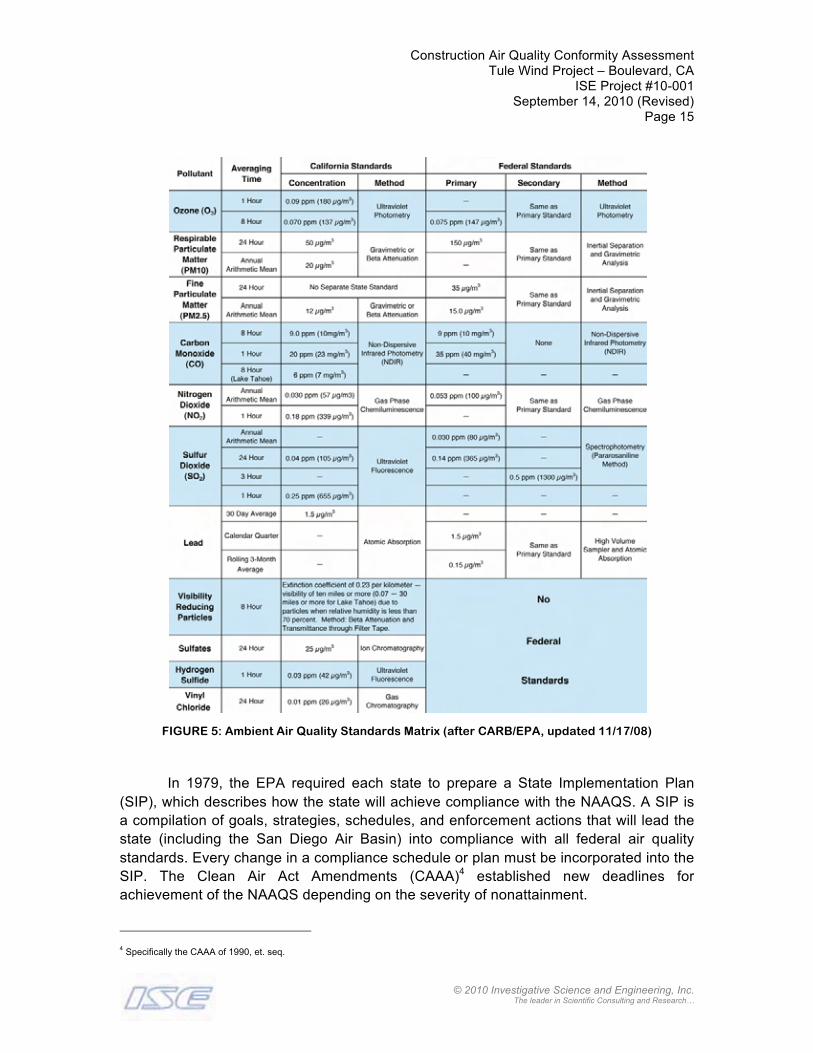
These standards are called the National Ambient Air Quality Standards (NAAQS).2 The California Air Resources Board (CARB) subsequently established the more stringent California Ambient Air Quality Standards (CAAQS).3 Both sets of standards are shown in Figure 5 on the following page. Areas in California where ambient air concentrations of pollutants are higher than the state standard are considered to be in “non-attainment”status for that pollutant.
THRESHOLDS OF SIGNIFICANCE
National Environmental Policy Act (NEPA) Thresholds
The EPA is responsible for enforcing the Federal Clean Air Act of 1970 (United States Code, Title 42, Chapter 85) and subsequent amendments. The Federal Clean Air Act (CAA) established the aforementioned NAAQS for the protection of human health and public welfare. The NAAQS represent the maximum levels of background pollution that provide an adequate margin of safety to protect the public health and welfare.
The CAA allows states to adopt ambient air quality standards and other regulations provided they are at least as stringent as federal standards. The California Clean Air Act of 1988 established CAAQS for criteria pollutants and additional standards for sulfates, hydrogen sulfide, vinyl chloride, and visibility reducing particles. CARB is the state regulatory agency with authority to enforce regulations to achieve and maintain the CAAQS, except in areas where the local air quality management district has been given authority over stationary source emissions. CARB required each air basin to develop its own strategy for achieving the NAAQS and CAAQS and still maintains regulatory authority over these strategies as well as mobile source emissions statewide.
The San Diego County Air Pollution Control District (SDAPCD) is the local agency for the administration and enforcement of air quality regulations; it adopted the Regional Air Quality Strategy (RAQS) to comply with CARB requirements for developing this plan.
2 Under the Federal Clean Air Act of 1970, U.S.C. Title 42, Chapter 85, as amended in 1977 and 1990.3 The new CARB eight-hour ozone standard became effective in early 2006. The new federal PM2.5 standard became effective in early 2007.
Construction Air Quality Conformity AssessmentTule Wind Project – Boulevard, CA
ISE Project #10-001September 14, 2010 (Revised)
Page 15
© 2010 Investigative Science and Engineering, Inc. The leader in Scientific Consulting and Research…
FIGURE 5: Ambient Air Quality Standards Matrix (after CARB/EPA, updated 11/17/08)
In 1979, the EPA required each state to prepare a State Implementation Plan (SIP), which describes how the state will achieve compliance with the NAAQS. A SIP is a compilation of goals, strategies, schedules, and enforcement actions that will lead the state (including the San Diego Air Basin) into compliance with all federal air quality standards. Every change in a compliance schedule or plan must be incorporated into the SIP. The Clean Air Act Amendments (CAAA)4 established new deadlines for achievement of the NAAQS depending on the severity of nonattainment.
4 Specifically the CAAA of 1990, et. seq.

Construction Air Quality Conformity AssessmentTule Wind Project – Boulevard, CA
ISE Project #10-001September 14, 2010 (Revised)
Page 16
© 2010 Investigative Science and Engineering, Inc. The leader in Scientific Consulting and Research…
The CAAA of 1990 also mandates states to develop an operating permit program that requires all major sources of pollutants to obtain an air permit, and contains programs designed to reduce mobile source emissions and control emissions of hazardous air pollutants through establishing control technology guidelines for various classes of sources.
Clean Air Act Conformity
On November 30, 1993, the EPA instituted final rules for determining generalconformity of federal actions with state and federal air quality implementation plans. Inorder to demonstrate conformity with the Clean Air Act, a project must clearly demonstrate that it does not:
1) Cause or contribute to any new violation of any standard in any area;
2) Increase the frequency or severity of any existing violation of any standard in any area; or,
3) Delay timely attainment of any standard, any required interim emission reductions, or other milestones in any area.
The conformity rule applies to federal actions in areas that violate one or more of the federal air quality standards (nonattainment areas). A conformity analysis is required for each of the nonattainment pollutants or its precursor emissions. The EPA has developed specific procedures for conformity determinations for federal actions, which include preparing an assessment of emissions associated with the action based on the most recent emission estimates.
New Source Review
A New Source Review (NSR) is required when a source has the potential to emit any pollutant regulated under the Clean Air Act in amounts equal to or exceeding specified major source threshold (100 or 250 tons per year) which are predicated on the source's industrial category. A major modification to the source also triggers the need for an NSR.
A major modification is a physical change or change in the method of operation at an existing major source that causes a significant "net emission increase" at that source of any pollutant regulated under the Clean Air Act. Any new or modified stationary emission sources require permits from the SDAPCD to construct and operate. Through the SDAPCD's permitting process, all stationary sources are reviewed and are subject to an NSR process. The NSR process ensures that factors such as the

Construction Air Quality Conformity AssessmentTule Wind Project – Boulevard, CA
ISE Project #10-001September 14, 2010 (Revised)
Page 17
© 2010 Investigative Science and Engineering, Inc. The leader in Scientific Consulting and Research…
availability of emission offsets and their ability to reduce emissions are addressed and conform with the SIP.
California Environmental Quality Act (CEQA) Thresholds
Section 15382 of the California Environmental Quality Act (CEQA) guidelines defines a significant impact as,
“… a substantial, or potentially substantial, adverse change in any of the physical conditions within the area affected by the project including land, air, water, minerals, flora, fauna, ambient noise, and objects of historic or aesthetic significance.”
The minimum change in ambient air quality conditions within the County of San Diego, as identified by the San Diego Air Pollution Control District’s implementation of the CAA is outlined below.
CEQA Air Quality Screening Standards The County of San Diego uses Appendix G.III of the State CEQA guidelines as
thresholds of significance, and recognizes the SDAPCD’s established screening thresholds for air quality emissions (Rules 20.1 et. seq.) as screening standards. These standards focus on the following potential impact areas, namely, would the project:
• Conflict with, or obstruct, implementation of the applicable air quality plan?
• Violate any air quality standard or contribute substantially to an existing or projected air quality violation?
• Result in a cumulatively considerable net increase of any criteria pollutant for which the project region is in non-attainment under an applicable federal or state ambient air quality standard (including releasing emissions which exceed quantitative thresholds for ozone precursors)?
• Expose sensitive receptors to substantial pollutant concentrations?
• Create objectionable odors affecting a substantial number of people?
These screening standards will be applied throughout this air quality conformity assessment for the basis of determination of both regional, as well as localized, air quality impacts due to the proposed project.
SDAPCD Criteria Pollutant Standards
Pursuant to the California Health & Safety Code, jurisdiction for regulation of air emissions from non-mobile sources within San Diego County (inclusive of the project site) has been delegated to the San Diego County Air Pollution Control District (APCD).5
5 Source: California Health & Safety Code, Division 26, Part 3, Chapter 1, Section §40002.

Construction Air Quality Conformity AssessmentTule Wind Project – Boulevard, CA
ISE Project #10-001September 14, 2010 (Revised)
Page 18
© 2010 Investigative Science and Engineering, Inc. The leader in Scientific Consulting and Research…
As part of its air quality permitting process, the APCD has established thresholds for the preparation of Air Quality Impact Assessments (AQIA’s) and/or Air Quality Conformity Assessments (AQCA’s).
APCD Rule 20.2, which outlines these screening level criteria, states that any project that results in an emission increase equal to or greater than any of these levels, must:
“… demonstrate through an AQIA . . . that the project will not (A) cause a violation of a State or national ambient air quality standard anywhere that does not already exceed such a standard, nor (B) cause additional violations of a national ambient air quality standard anywhere the standard is already being exceeded, nor (C) cause additional violations of a State ambient air quality standard anywhere the standard is already being exceeded, nor (D) prevent or interfere with the attainment or maintenance of any State or national ambient air quality standard.”
The applicable standards are shown in Table 1 below. For projects whose source emissions are below these criteria, no AQIA is typically required, and project level emissions are presumed to be less than significant. The County of San Diego accepts the use of these “screening criteria” as “Thresholds of Significance” by projects for the purposes of CEQA analysis.
TABLE 1: Thresholds of Significance for Air Quality Impacts
PollutantSDAPCD Thresholds of
Significance(Pounds per Day)
Clean Air Act less than significantLevels (Tons per Year)
Carbon Monoxide (CO) 550 100
Oxides of Nitrogen (NOx) 250 50
Oxides of Sulfur (SOx) 250 100
Particulate Matter (PM10) 100 100
Particulate Matter (PM2.5) 55 100
Volatile / Reactive Organic Compounds & Gasses (VOC/ROG) 75 50
Source: SDAPCD Rule 1501, 20.2(d)(2), 1995; EPA 40 CFR 93, 1993.
• Threshold for VOC’s based on the threshold of significance for reactive organic gases (ROG’s) from Chapter 6 of the CEQA Air Quality Handbook of the South Coast Air Quality Management District.
• Threshold for ROG’s in the eastern portion of the County based on the threshold of significance for reactive organic gases(ROG’s) from Chapter 6 of the CEQA Air Quality Handbook of the Southeast Desert Air Basin.
• Thresholds are applicable for either construction or operational phases of a project action.
• The PM2.5 threshold is based upon the proposed standard identified in the, “Final – Methodology to Calculate Particulate Matter (PM) 2.5 and PM 2.5 Significance Thresholds”, published by SCAQMD in October 2006.

Construction Air Quality Conformity AssessmentTule Wind Project – Boulevard, CA
ISE Project #10-001September 14, 2010 (Revised)
Page 19
© 2010 Investigative Science and Engineering, Inc. The leader in Scientific Consulting and Research…
Under the General Conformity Rule, the EPA has developed a set of de minimisthresholds for all proposed federal actions in a non-attainment area for evaluating the significance of air quality impacts. It should be noted that the State (i.e., SDAPCD)standards are equal to, or more stringent than, the Federal Clean Air standards and would be applicable under the CAA.6 Development of the proposed project would therefore fall under the stricter SDAPCD guidelines.
These guidelines are compatible with those utilized elsewhere in the State (such as South Coast Air Quality Management District standards, etc.) as part of CEQA guidance documents. In the event that project emissions may approach or exceed these screening level criteria, modeling would be required to demonstrate that the project’s ground-level concentrations, including appropriate background levels, are below the Federal and State Ambient Air Quality Standards.
For a conformity analysis, the existing ambient conditions are compared for the
with- and without-project cases. If emissions exceed the allowable thresholds, additional analysis is conducted to determine whether the emissions would exceed an ambient air quality standard (i.e., the CAAQS values previously shown in Figure 5). Determination of significance considers both localized impacts (such as CO hotspots) and cumulative impacts. In the event that any criteria pollutant exceeds the threshold levels, the proposed action’s impact on air quality is considered significant and mitigation measures would be required.
For CEQA purposes, these screening criteria are used as numeric methods to demonstrate that a project’s total emissions (e.g. stationary and fugitive emissions, as well as emissions from mobile sources) would not result in a significant impact to air quality. Since APCD does not have AQIA thresholds for emissions of volatile organic compounds (VOC’s), the use of the screening level for reactive organic compounds (ROC) from the CEQA Air Quality Handbook for the South Coast Air Basin (SCAB), which has stricter standards for emissions of ROC’s/VOC’s than San Diego’s, is appropriate. No differentiation is made between construction and operational emission thresholds within the SDAPCD.
6 A fact that can be verified through multiplication of the SDAPCD standards by 365 days and dividing by 2,000 pounds.

Construction Air Quality Conformity AssessmentTule Wind Project – Boulevard, CA
ISE Project #10-001September 14, 2010 (Revised)
Page 20
© 2010 Investigative Science and Engineering, Inc. The leader in Scientific Consulting and Research…
Combustion Toxics Risk Factors
When fuel burns in an engine, the resulting exhaust is made up of soot and gases representing hundreds of different chemical substances. The predominant constituents are:
o Nitrous Oxide o Nitrogen Dioxideo Formaldehyde o Benzeneo Sulfur Dioxide o Hydrogen Sulfideo Carbon Dioxide o Carbon Monoxide
Over ninety-percent (90%) of the exhaust emissions from an engine consist of soot particles whose size is equal to, or less than, 10-microns in diameter. Particles of this size can easily be inhaled and deposited in the lungs. Diesel exhaust contains roughly 20 to 100 times more emissive particles than gasoline exhaust. Of principal concern are particles of cancer causing substances known as polynuclear aromatic hydrocarbons (PAH’s).7
There are inherent uncertainties in risk assessment with regard to the identification of compounds as causing cancer or other adverse health effects in humans, the cancer potencies and Reference Exposure Levels (REL’s)8 of compounds, and the exposure that individuals receive. It is common practice to use conservative (health protective) assumptions with respect to uncertain parameters. The uncertainties and conservative assumptions must be considered when evaluating the results of risk assessments.
Since the potential health effects of contaminants are commonly identified based on animal studies, there is uncertainty in the application of these findings to humans. In addition, for many compounds it is uncertain whether the health effects observed at higher exposure levels in the laboratory or in occupational settings will occur at lower environmental exposure levels. In order to ensure that potential health impacts are not underestimated, it is commonly assumed that effects seen in animals, or at high exposure levels, could potentially occur in humans following low-level environmental exposure.
7 Polynuclear aromatic hydrocarbons (PAH’s) are hydrocarbon compounds with multiple benzene rings. PAH’s are a group of approximately 10,000 compounds which result predominately from the incomplete burning of carbon-containing materials like oil, wood, garbage or coal.8 The exposure level at which there are no biologically significant increases in the frequency or severity of adverse effects between the exposed population and the control group. Some effects may be produced at this level, but they are not considered adverse or precursors to adverse effects.

Construction Air Quality Conformity AssessmentTule Wind Project – Boulevard, CA
ISE Project #10-001September 14, 2010 (Revised)
Page 21
© 2010 Investigative Science and Engineering, Inc. The leader in Scientific Consulting and Research…
Estimates of potencies and REL’s are derived from experimental animal studies, or from epidemiological studies of exposed workers or other populations.9 Uncertainty arises from the application of potency, or REL values derived from this data, to the general human population. There is debate as to the appropriate levels of risk assigned to diesel particulates, since the USEPA has not yet declared diesel particulates as a toxic air contaminant.
Using the CARB threshold, a risk concentration level of one in one million (1:1,000,000) of continuous 70-year exposure is considered less than significant. A risk exposure level of ten in one million (10:1,000,000) is acceptable if Toxic Best Available Control Technologies (T-BACT’s) are used. It should be noted that this type of reporting is only strictly applicable to large populations (such as entire air basins), where the sample group is sizeable, and the exposure time is long (which is not the case for project-level construction projects).
For purposes of analysis under this report, and to be consistent with the approaches used for other toxic pollutants, a functional comparison of the aforementioned risk probability per individual person exposed to construction contaminants will be examined. This approach has the advantage of not needing to quantify the population of the statistical group adjacent to the construction (which could yield false values), as well as allowing the per-person risk to be expressed as a final percentage (with a percentage level of 100% being equal to the impact threshold). Of course, for a large enough population sample (i.e., a million people or more) the results are identical to CARB’s prediction methodology.
ANALYSIS METHODOLOGY
The analysis criteria for air quality impacts are based upon the approach recommended by the South Coast Air Quality Management District’s (SCAQMD) CEQAHandbook.10 The handbook establishes aggregate emission calculations for determining the potential significance of a proposed action. In the event that the emissions exceed the established thresholds, air dispersion modeling may be conducted to assess whether the proposed action results in an exceedance of an air quality standard. The County of San Diego has adopted this methodology.
9 Source: CalEPA, USEPA, SCAQMD, 2001 et. seq.10 The SCAQMD CEQA Handbook is a reference volume containing an extensive list of semi-empirical (quantified experimental) curve-fitequations describing various emissive sources having important context under CEQA. The equations are not perfect (in that they would not constitute an ‘exact solution’ in a scientific sense), but are nonetheless a reasonable approximation of the physical problem. In the same light, programs which utilize the SCAQMD semi-empirical methodology (such as URBEMIS 2007 and the like) provide no greater problem understanding than using the equations directly. Such programs are still subject to all of the same limitations as the methods and equations on which they rely.

Construction Air Quality Conformity AssessmentTule Wind Project – Boulevard, CA
ISE Project #10-001September 14, 2010 (Revised)
Page 22
© 2010 Investigative Science and Engineering, Inc. The leader in Scientific Consulting and Research…
Ambient Air Quality Data Collection
CARB Air Monitoring Station Data within Project Vicinity
The California Air Resources Board (CARB) monitors ambient air quality at approximately 250 air-monitoring stations across the state. Air quality monitoring stations usually measure pollutant concentrations 10 feet above ground level; therefore, air quality is often referred to in terms of ground-level concentrations. Ambient air pollutant concentrations are measured at 10 air-quality-monitoring stations operated by the SDAPCD. Neighboring Imperial County Air Pollution Control District (ICAPCD) maintains seven air-quality-monitoring stations operated by either ICAPCD or CARB.
Two ambient air-quality-monitoring stations (denoted by the symbol in Figure 6 on the following page), which are in relatively close proximity to the project site, and would be representative of ambient air toxics under both onshore and offshore atmospheric wind conditions, are located within the San Diego air basin11 approximately 26.7 miles from the project site (Alpine Monitoring Station denoted by the red circle), and within the Salton Sea Air Basin12 approximately 43.8 miles distant (El Centro Monitoring Station denoted by the blue circle). Given the location of the project site with respect to the eastern San Diego desert regions, the El Centro monitoring station has high significance, due to the dominant high pressure condition driving offshore flow past the project site due to extreme temperatures within this region.
The Alpine monitoring station currently records NO2, O3 and PM2.5, while the El Centro monitoring station records a larger selection of criteria pollutants consisting of CO, NO2, O3, PM10 and PM2.5. Both stations record various meteorological parameters, such as barometric pressure, wind speed, etc. Other stations within the project vicinity present either incomplete or redundant data, or were determined not to be representative of localized ambient air quality conditions present at the project site.
Finally, due to the type of equipment employed at each station, not every station is capable of recording the entire set of criteria pollutants previously identified in Table 1. Periodic audits are conducted to ensure calibration conformance.13
11 Alpine Monitoring Station (2300 Victoria Dr, Alpine CA 91901) – ARB Station ID 80128. 12 El Centro Monitoring Station (150 9th St, El Centro CA 92243) – ARB Station ID 13694. 13 Calibration of CARB equipment is performed in accordance with the U.S. Environmental Protection Agency's 40 CFR, Part 58, Appendix A protocol with all equipment traceable to National Institute of Standards and Technology (NIST) standards. The typical accuracy of the equipment is ±15% for gasses (such as CO, NOx, etc.) and ±10% for PM10.

Construction Air Quality Conformity AssessmentTule Wind Project – Boulevard, CA
ISE Project #10-001September 14, 2010 (Revised)
Page 23
© 2010 Investigative Science and Engineering, Inc. The leader in Scientific Consulting and Research…
FIGURE 6: Ambient Air Quality Monitoring Station Location Map (ISE 9/10)
Construction Air Quality Conformity AssessmentTule Wind Project – Boulevard, CA
ISE Project #10-001September 14, 2010 (Revised)
Page 24
© 2010 Investigative Science and Engineering, Inc. The leader in Scientific Consulting and Research…
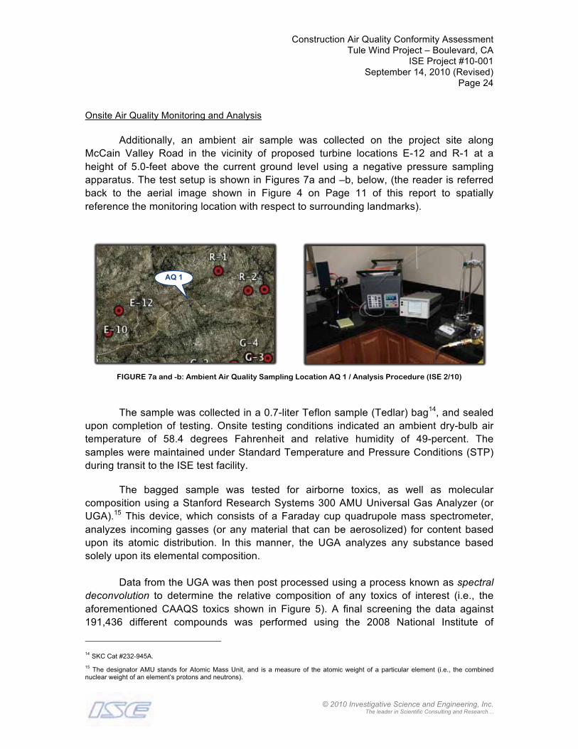
Onsite Air Quality Monitoring and Analysis
Additionally, an ambient air sample was collected on the project site along McCain Valley Road in the vicinity of proposed turbine locations E-12 and R-1 at a height of 5.0-feet above the current ground level using a negative pressure sampling apparatus. The test setup is shown in Figures 7a and –b, below, (the reader is referredback to the aerial image shown in Figure 4 on Page 11 of this report to spatially reference the monitoring location with respect to surrounding landmarks).
FIGURE 7a and -b: Ambient Air Quality Sampling Location AQ 1 / Analysis Procedure (ISE 2/10)
The sample was collected in a 0.7-liter Teflon sample (Tedlar) bag14, and sealed upon completion of testing. Onsite testing conditions indicated an ambient dry-bulb air temperature of 58.4 degrees Fahrenheit and relative humidity of 49-percent. The samples were maintained under Standard Temperature and Pressure Conditions (STP)during transit to the ISE test facility.
The bagged sample was tested for airborne toxics, as well as molecular composition using a Stanford Research Systems 300 AMU Universal Gas Analyzer (or UGA).15 This device, which consists of a Faraday cup quadrupole mass spectrometer,analyzes incoming gasses (or any material that can be aerosolized) for content based upon its atomic distribution. In this manner, the UGA analyzes any substance based solely upon its elemental composition.
Data from the UGA was then post processed using a process known as spectral deconvolution to determine the relative composition of any toxics of interest (i.e., the aforementioned CAAQS toxics shown in Figure 5). A final screening the data against 191,436 different compounds was performed using the 2008 National Institute of
14 SKC Cat #232-945A. 15 The designator AMU stands for Atomic Mass Unit, and is a measure of the atomic weight of a particular element (i.e., the combined nuclear weight of an element’s protons and neutrons).
AQ 1

Construction Air Quality Conformity AssessmentTule Wind Project – Boulevard, CA
ISE Project #10-001September 14, 2010 (Revised)
Page 25
© 2010 Investigative Science and Engineering, Inc. The leader in Scientific Consulting and Research…
Standards and Technology (NIST08) Mass Spectral Library search program. The spectrometer test setup is shown in the second photo pane of Figure 7, above. Construction Air Quality Modeling
Construction Vehicle Emission Modeling (CO, NOx, SOx, PM10, PM2.5, ROG)
Primary construction vehicle pollutant emission generators expected within the Tule Wind Project development site would consist predominately of diesel-powered grading equipment required for grading activities, surface preparation, and ultimate tower construction. The analysis methodology utilized in this report is based upon the EPA AP-42 source emissions report for the various classes of diesel construction equipment.16
The generation rates of typical equipment are identified in Table 2 on the following page, and would constitute the baseline (unmitigated, or Tier 0) construction emission rates. Estimates of daily load factors (i.e., the amount of time during a day that any piece of equipment is under load) were based upon past ISE engineering experience with similar operations, and consultation with the project applicant.
In cases where the required construction equipment aggregate does not comply with the applicable standards for a pollutant under examination, mitigation is imposed by requiring cleaner Tier 1 through 4 equipment, as required under the Federal Clean Air Act.17,18 These maximum emission rates are shown as footnotes to Table 2 for CO, NOx
and PM10 for Tier 2 or better (denoted as Tier 2+) equipment.19 Additional recommendations for “Blue Sky Series” equipment will be made if the applicant cannot demonstrate strict Tier 2+ compliance.20
16 This tabulation provided by the EPA is the foundation of all construction emission programs available by CARB, such as OFFROAD and the like. This equipment list would be classified as Tier Zero (Tier 0) equipment having none of the emissions control technologies required under the newer Tier 1 through 3 programs. This is the case for older construction equipment that is sometimes used on project sites.17 Source: US Code of Federal Regulations, Title 40, Part 89 [40 CFR Part 89].18 In most cases the federal regulations for diesel construction equipment also apply in California, whose authority to set emission standards for new diesel engines is limited. The federal Clean Air Act Amendments of 1990 (CAA) preempt California’s authority to control emissions from both new farm and construction equipment under 175 hp [CAA Section 209(e)(1)(A)] and require California to receive authorization from the federal EPA for controls over other off-road sources [CAA Section 209 (e)(2)(A)]. 19 Again, for the purposes of mitigation, any construction equipment unable to comply with the applicable standards for a specific pollutant will be reanalyzed using the applicable Tier 2 equipment for engine sizes over 50 HP. These emission rates became mandatory for all equipment built starting 2001 or later (depending on engine size).20 The “Blue Sky Series” designation [40 CFR Part 89] is a voluntary program enacted by the USEPA requiring participating engine manufacturers to produce cleaner burning engines that are at least 40% better than current Tier 2 or 3 mandates. Engines with this designation are assumed by the EPA to produce de facto compliance with current and future air quality emissions standards. This program also exists for recreational and commercial marine diesel engines [40 CFR Part 94] and land-based non-road spark-ignition engines over 25 HP [40 CFR Part1048].

Construction Air Quality Conformity AssessmentTule Wind Project – Boulevard, CA
ISE Project #10-001September 14, 2010 (Revised)
Page 26
© 2010 Investigative Science and Engineering, Inc. The leader in Scientific Consulting and Research…
TABLE 2: Baseline ‘Tier 0’ AP-42 Equipment Pollutant Generation Rates21
Generation Rates (pounds per horsepower-hour)
Equipment Class CO NOx SOx PM10 PM2.5 ROG
Track Backhoe 0.0150 0.0220 0.0020 0.0010 0.0009 0.0030
Dozer - D8 Cat 0.0150 0.0220 0.0020 0.0010 0.0009 0.0030
Hydraulic Crane 0.0090 0.0230 0.0020 0.0015 0.0014 0.0030
Loader/Grader 0.0150 0.0220 0.0020 0.0010 0.0009 0.0030
Side Boom 0.0130 0.0310 0.0020 0.0015 0.0014 0.0030
Water Truck 0.0060 0.0210 0.0020 0.0015 0.0014 0.0020
Concrete Truck 0.0060 0.0210 0.0020 0.0015 0.0014 0.0020
Concrete Pump 0.0110 0.0180 0.0020 0.0010 0.0009 0.0020
Dump/Haul Trucks 0.0060 0.0210 0.0020 0.0015 0.0014 0.0020
Paver / Blade 0.0070 0.0230 0.0020 0.0010 0.0009 0.0010
Roller / Compactor 0.0070 0.0200 0.0020 0.0010 0.0009 0.0020
Scraper 0.0110 0.0190 0.0020 0.0015 0.0014 0.0010
Emissions Reduction Mandates:
o The maximum CO emissions from Tier 2 equipment is 0.0082 pounds per horsepower-hour (lb/HP-hr) for equipment with power ratings between 50 and 175 HP, and 0.0057 lb/HP-hr for equipment with power ratings over 175 HP. Tier 3 ratings only apply between 50 to 750 HP and are identical to Tier 2 requirements. Tier 4 requirements (to be phased-in between 2008 and 2015) set a sliding scale on CO limits ranging from 0.0132 lb/HP-hr for small engines, to 0.0057 lb/HP-hr for engines up to 750 HP.
o The maximum NOx and PM10 emissions from Tier 2 equipment are 0.0152 and 0.0003 lb/HP-hr regardless of the engine size. Tier 3 emissions must meet the Tier 2 requirement. Tier 4 standards further reduce this level to 0.0006 lb/HP-hr for NOx, and0.00003 lb/HP-hr for PM10 for engines over 75 HP.
Table data sourced U.S. EPA AP-42 “Compilation of Air Pollutant Emission Factors”, 9/85 through present.
Ratings shown for full (100%) load factor.
Finally, fine particulate dust generation (PM2.5) from construction equipment was analyzed using the methodology identified by the SCAQMD and utilized by the SDAPCD.22 This approach, which utilizes the California Emission Inventory Development and Reporting System (CEIDARS) database, estimates PM2.5 emissions as a fractional percentage of the aggregate PM10 emissions. For diesel construction equipment, the fractional emission factor is 0.920 PM2.5 / PM10.
Fugitive Dust Emission Modeling (PM10, PM2.5)
Fugitive dust generation from the proposed grading plan was analyzed using the methodology recommended in the SCAQMD CEQA Handbook guidelines for calculating 10-micron Particulate Matter (PM10) due to earthwork movement and stockpiling. The analysis assumed low-wind speeds and active wet suppression control. Aggregate levels
21 The PM2.5 emission factors are based upon the SCAQMD document, “Final – Methodology to Calculate Particulate Matter (PM) 2.5 and PM 2.5 Significance Thresholds”, 10/06. The correction factor for diesel equipment of this type is 0.920.22 The source citation is: “Methodology to Calculate Particulate Matter (PM) 2.5 and PM2.5 Significance Thresholds”, October 2006.
Construction Air Quality Conformity AssessmentTule Wind Project – Boulevard, CA
ISE Project #10-001September 14, 2010 (Revised)
Page 27
© 2010 Investigative Science and Engineering, Inc. The leader in Scientific Consulting and Research…
of PM10, based upon the best available surface grading estimates, were calculated in pounds per day and compared to the applicable significance criteria previously shown in Table 1.
For surface grading operations, the fractional emission factor is 0.208 PM2.5 / PM10 based upon the SCAQMD approach. For unpaved road travel, the fractional emission factor is 0.212 PM2.5 / PM10.
Combustion-Fired Health-Risk Emission Modeling (PM10, PM2.5)
For the purposes of this analysis, construction vehicle pollutant emission generators would consist entirely of construction activities associated with onsite clearing and grading operations (which is the worst-case pollution emission scenario). The analysis methodology utilized in this report is based upon EPA and CARBguidelines for construction operations. Construction emissions were based upon the previously identified EPA Tier 0 through Tier 2+ generation rates for the various classes of diesel construction equipment.
A screening risk assessment of diesel-fired toxics from construction equipment was performed using the SCREEN3 dispersion model developed by the EPA’s Office of Air Quality Planning and Standards.23 The SCREEN3 model uses a Gaussian plume dispersion algorithm that incorporates source-related and meteorological factors to estimate pollutant concentration from continuous sources.
It is assumed that the pollutant does not undergo any chemical reactions, and
that no other removal processes, such as wet or dry deposition, act on the plume during its transport from the source.
Using the concentrations obtained from the screening model, the diesel toxic riskcan be defined as shown below:
Risk =Fwind × EMFAC ×URF70 year exposure
Dilution
where, Risk is the excess cancer risk (probability in one-million);Fwind is the frequency of the wind blowing from the exhaust source to the receptor (the default
value is 1.0);EMFAC is the exhaust particulate emission factor (the level from the screening model); URF70 year exposure is the Air Resource Board unit risk probability factor (300 x 10-6, or 300 in a
million cancer risk per µg/m3 of diesel combustion generated PM10 inhaled in a 70-year
23 The methodology is based upon the Industrial Source Complex (ISC3) source dispersion approach as outlined in the EPA-454/B-95-003btechnical document. The SCREEN3 model is used within the State of California and is typically more restrictive than the ISC3 model.

Construction Air Quality Conformity AssessmentTule Wind Project – Boulevard, CA
ISE Project #10-001September 14, 2010 (Revised)
Page 28
© 2010 Investigative Science and Engineering, Inc. The leader in Scientific Consulting and Research…
lifetime based upon ARB 1999 Staff Report from the Scientific Review Panel (SRP) on Diesel Toxics); and,
Dilution is the atmospheric dilution ratio during source-to-receptor transport (the default value of 1.0 assumes no dilution)
Given the above assumptions for wind frequency and atmospheric dilution ratio, and substituting the CARB recommended value for the unit risk probability factor, gives the following expression:
Risk = 1× EMFAC × 300x10−6
1= 300x10−6 × EMFAC per person
Thus, the percentage of risk of cancer to any given person, being exposed to a
concentration of pollution equal to EMFAC (in µg/m3) over a continuous period of 70-years, would be:
Risk(%) = (300x10−6 × EMFAC) ×100 = 300x10−4 × EMFAC per person
Where it can be directly stated that a risk percentage of, say, 25% would indicate a 25% probability of inhaled cancer risk for the given level of exposure if consumed continuously for a period of 70-years. A 50% probability would correspond to a 50:50 chance of inhaled cancer risk if consumed continuously for a period of 70-years, and so on.
For the construction-related diesel-fired toxics analysis, an area-source consistent in dimensions with the proposed grading area will be assumed. A simplified elevated terrain model (which is consistent with the area surrounding the project site) with no building downwash corrections and a worst-case wind direction was utilized.
Aggregate Vehicle Emission Air Quality Modeling
Motor vehicles emissions associated with construction worker trips for the proposed Tule Wind Project development were calculated by multiplying the appropriate emission factor (in grams per mile) times the estimated trip length and the total number of vehicles. Appropriate conversion factors were then applied to provide aggregate emission units of pounds per day. CARB estimates on-road motor vehicle emissions by using a series of models called the Motor Vehicle Emission Inventory (MVEI) Models.
Construction Air Quality Conformity AssessmentTule Wind Project – Boulevard, CA
ISE Project #10-001September 14, 2010 (Revised)
Page 29
© 2010 Investigative Science and Engineering, Inc. The leader in Scientific Consulting and Research…
Four computer models, which form the MVEI, are CALIMFAC, WEIGHT, EMFAC, and BURDEN.24 They function as follows:
o The CALIMFAC model produces base emission rates for each model year when a vehicle is new and as it accumulates mileage and the emission controls deteriorate.
o The WEIGHT model calculates the relative weighting each model year should be given in the total inventory, and each model year's accumulated mileage.
o The EMFAC model uses these pieces of information, along with the correction factors and other data, to produce fleet composite emission factors.
o Finally, the BURDEN model combines the emission factors with county-specific activity data to produce to emission inventories.
For the current analysis, the EMFAC 2007 Model v2.3 of the MVEI25 was run using input conditions specific to the San Diego County air basin to predict construction worker vehicle emissions from the project based upon a near term year 2012 scenario.26
The aggregate emission factors from the CARB EMFAC 2007 model are provided as an attachment at the end of this report.
Additionally, a mix ratio consistent with the Caltrans ITS Transportation Project-Level Carbon Monoxide Protocol was used. This consisted of the following air standardOtto-Cycle engine vehicle distribution percentages:
Light Duty Autos = 69.0 Light Duty Trucks = 19.4Medium Duty Trucks = 6.4 Heavy Duty Trucks = 4.7
Buses = 0.0 Motorcycles = 0.5
Fine particulate dust generation (PM2.5) from motor vehicle operation was analyzed using the methodology identified by SCAQMD27. This approach, which utilizes the California Emission Inventory Development and Reporting System (CEIDARS)database, estimates PM2.5 emissions as a fractional percentage of the aggregate PM10
emissions. For vehicular traffic, the fractional emission factor is 0.998 PM2.5 / PM10
based upon the SCAQMD approach.
24 The module named EMFAC should not be confused with the entire EMFAC 2007 program itself (which calls the subroutines CALIMFAC, WEIGHT, EMFAC, and BURDEN to determine the final emission inventory for a particular area).25 This is the most current CARB emissions model approved for use within the State of California.26 This is a worst-case assumption, since implementation of cleaner vehicle controls ultimately reduces emissions under future year conditions. By applying near-term emission factors to the complete project, an upper bound on project-related emissions is obtained.27 This is detailed in the document entitled, “Final Methodology to Calculate Particulate Matter (PM) 2.5 and PM2.5 Significance Thresholds”,published by SCAQMD.

Construction Air Quality Conformity AssessmentTule Wind Project – Boulevard, CA
ISE Project #10-001September 14, 2010 (Revised)
Page 30
© 2010 Investigative Science and Engineering, Inc. The leader in Scientific Consulting and Research…
Vehicular CO / NOx / PM10 / PM2.5 Conformity Assessment
A hotspot conformity analysis was performed on all project-related roadway
segments, using the California Line Source Emissions Model Version 4 (CALINE4)28 air dispersion model methodology in order to quantify near term cumulative plus projectpollutant concentrations within this portion of the project air basin. CALINE4 is the accepted line source dispersion model within the State of California.
For the hotspot analysis, horizon traffic volumes for all affected roadway segments were used based upon values provided by the project traffic engineer.29,30
Worst case mean running speeds of 45 MPH were used for all potentially impacted roadway segments utilizing the aforementioned Caltrans ITS Transportation Project-Level Carbon Monoxide Protocol mix ratios per EMFAC 2007. Worst-case wind speed, aggregate emissions class data, and meteorological assumptions were created and run for various traffic scenarios. The peak hour traffic volume was calculated at worst-case 10-percent of the daily ADT.
This produced the following worst-case running emission factors, which can be
seen in the last column of the EMFAC output:
CO = 2.511 grams/mile
NOx = 0.729 grams/mile
PM10 = 0.023 grams/mile
Ambient CO and PM10 concentrations were determined through the previously discussed field monitoring effort. Levels for NOx precursors were set to either the field monitored values or the basin-wide levels (whichever is greater). The NO2 photolysis rate was taken at a default atmospheric solar value of 0.004/sec.31 The CALINE4solution space results for each pollutant is provided as attachments to this report.
28 CALINE4 is a Gaussian line dispersion model, developed by Caltrans; it is used to predict localized vehicle emissions from mobile sources. The model uses source strength, meteorological data, and site geometry to predict pollutant concentrations within 1,500 feet of the roadway.29 These levels are expected to occur sometime between the near term condition and the ultimate horizon year 2030. To ensure a worst-case analysis, these levels will be applied against the near term emission factors.30 Source: Full Traffic Impact Study – Tule Wind Farm, LLG, Inc., 3/26/10.31 Photolysis is the process by which a chemical compound undergoes a change in valence as the result of the absorption of a photon (i.e., light). This process is also called photodecomposition, photochemical reaction, or photo-oxidation.

Construction Air Quality Conformity AssessmentTule Wind Project – Boulevard, CA
ISE Project #10-001September 14, 2010 (Revised)
Page 31
© 2010 Investigative Science and Engineering, Inc. The leader in Scientific Consulting and Research…
FINDINGS
Existing Climate Conditions
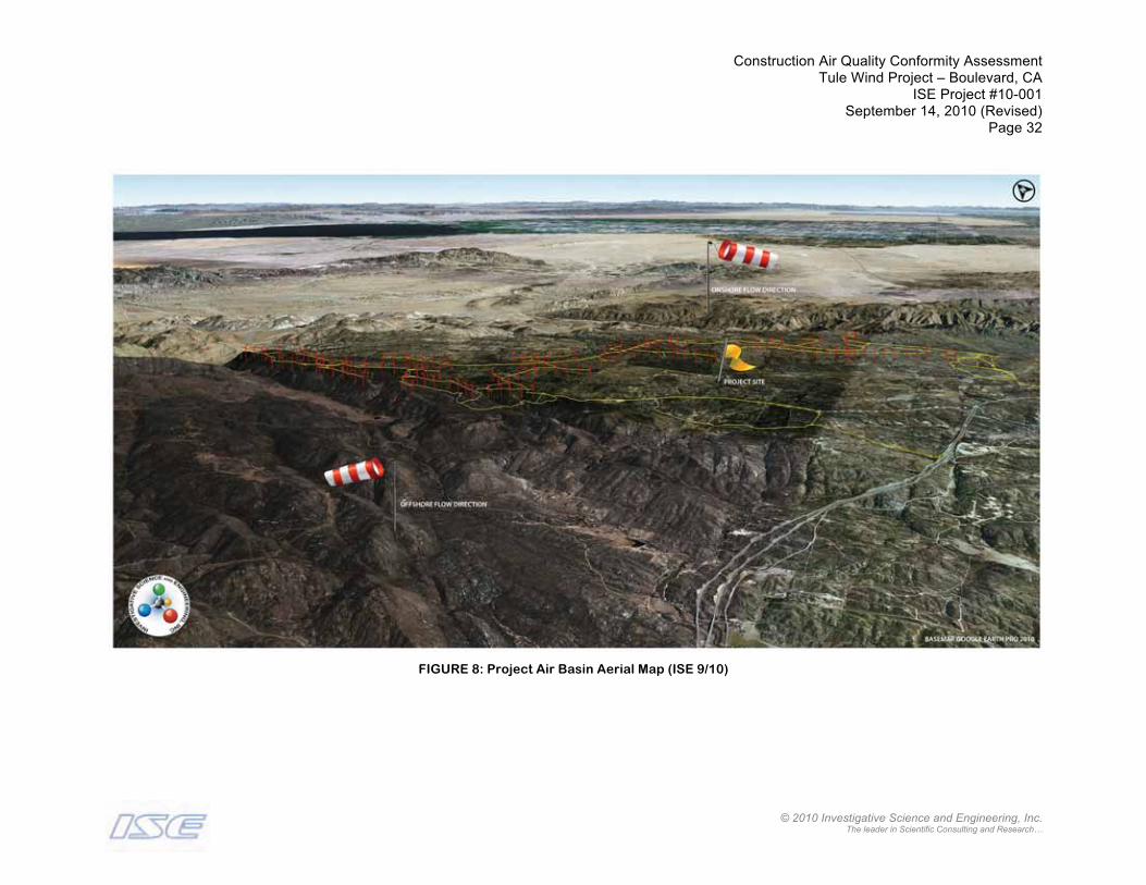
The climate within the region surrounding the proposed Tule Wind Project development site is characterized by warm, dry summers and mild, wet winters; it is dominated by a semi-permanent high-pressure cell located over the Pacific Ocean. This high-pressure cell maintains clear skies over the air basin for much of the year. It also drives the dominant onshore circulation, as can be seen in Figure 8 on the following page, and helps to create two types of temperature inversions, subsidence and radiation, that contribute to local air quality degradation.
Subsidence inversions occur during the warmer months, as descending air associated with the Pacific high-pressure cell meets cool marine air. The boundary between the two layers of air represents a temperature inversion that traps pollutants below it. Radiation inversion typically develops on winter nights, when air near the ground cools by radiation, and the air aloft remains warm. A shallow inversion layer that can trap pollutants is formed between the two layers.
Frequently, the strongest winds in the basin occur during the night and morning hours due to the absence of onshore sea breezes. The overall result is a noticeable degradation in local air quality.32
Finally, in the area of the proposed project site, the maximum and minimum average temperatures are 94º F and 32º F, respectively.33 Precipitation in the area averages 15.6 inches annually, 90 percent of which falls between November and April. The prevailing wind direction is from the west-northwest, with an annual mean speed of 6 to 10 miles per hour. Sunshine is usually plentiful in the proposed project area but night and morning cloudiness is common during the spring and summer. Fog can occasionally develop during the winter.
32 Occasionally during the months of October through February, offshore flow becomes a dominant factor in the regional air quality. These periods, known as “Santa Ana Conditions”, are typically maximal during the month of December with wind speeds from the north to east approaching 35 knots and gusting to over 50 knots. This air movement is caused by clockwise pressure circulation over the Great Basin (i.e., the high plateau east of the Sierra Mountains and west of the Rocky Mountains including most of Nevada and Utah), which results in significant downward air motion towards the ocean. Stronger Santa Ana winds can have gusts greater than 60 knots over widespread areas and gusts greater than 100 knots in canyon areas.33 Source: National Weather Service (NWS) / National Oceanographic and Atmospheric Administration (NOAA), 2010.
Construction Air Quality Conformity AssessmentTule Wind Project – Boulevard, CA
ISE Project #10-001September 14, 2010 (Revised)
Page 32
© 2010 Investigative Science and Engineering, Inc. The leader in Scientific Consulting and Research…
FIGURE 8: Project Air Basin Aerial Map (ISE 9/10)

Construction Air Quality Conformity AssessmentTule Wind Project – Boulevard, CA
ISE Project #10-001September 14, 2010 (Revised)
Page 33
© 2010 Investigative Science and Engineering, Inc. The leader in Scientific Consulting and Research…
Existing Air Quality Levels
CARB Aerometric Station Data within Project Vicinity
The project site is located in the central portion of the San Diego Air Basin. The Basin continues to have a transitional-attainment status of federal standards for Ozone(O3) and PM10. The Basin is either in attainment or unclassified for federal standards of CO, SO2, NO2, and lead. Factors affecting ground level pollutant concentrations include the rate at which pollutants are emitted to the atmosphere, the height from which they are released, and topographic and meteorological features.
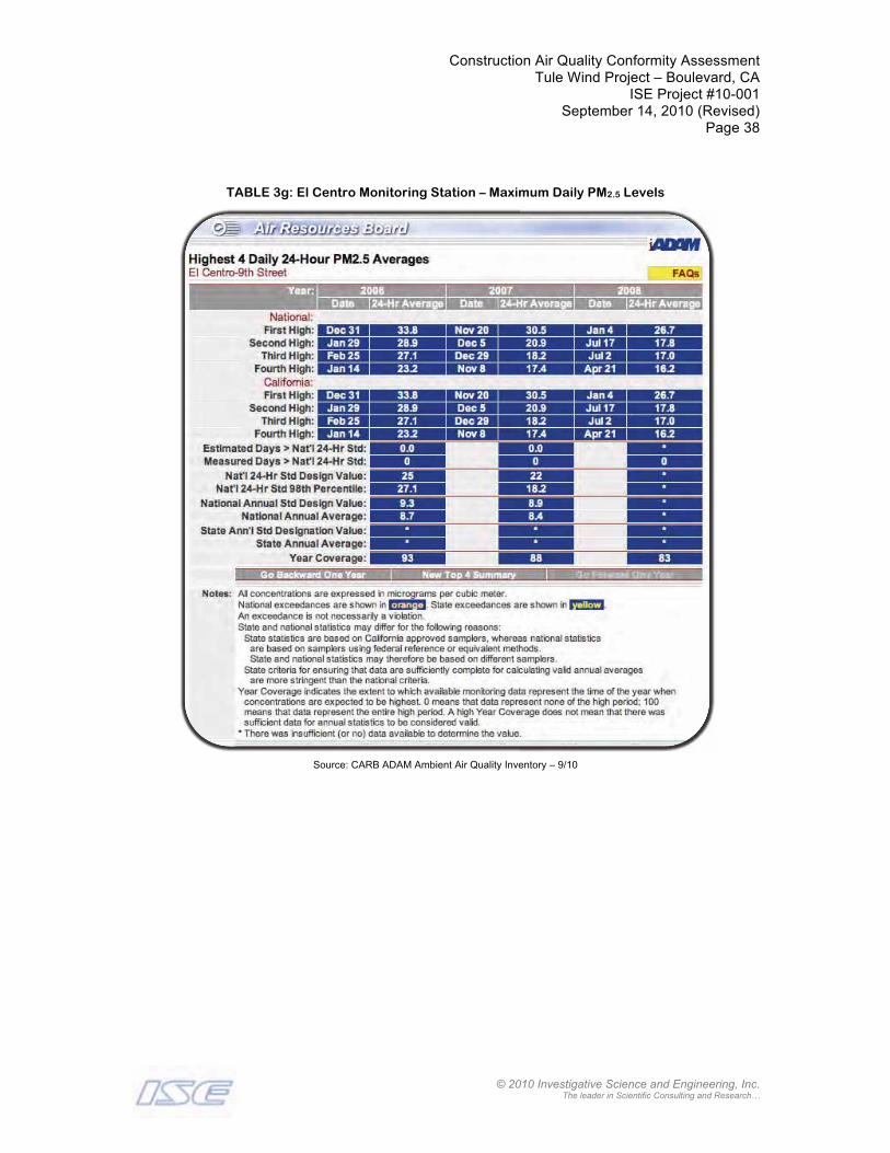
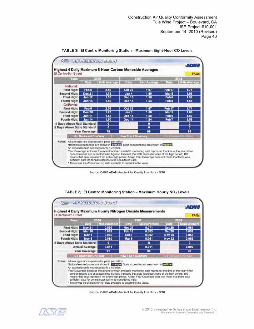
Tables 3a through -j, starting below, provide a summary of the highest pollutant levels recorded at the previously identified monitoring stations for the last year available (2008), based upon the latest data from the CARB Aerometric Data Analysis and Management (ADAM) System database. Given these factors, the closest monitoring stations reported exceedances for O3, and PM10 (although it will be shown shortly that these exceedances did not translate to appreciable levels at the project site). All other criteria pollutants were within both federal and state standards, or not monitored.34
TABLE 3a: Alpine Monitoring Station – Maximum Hourly O3 Levels
Source: CARB ADAM Ambient Air Quality Inventory – 9/10
34 Monitoring for lead was discontinued entirely in 1998.

Construction Air Quality Conformity AssessmentTule Wind Project – Boulevard, CA
ISE Project #10-001September 14, 2010 (Revised)
Page 34
© 2010 Investigative Science and Engineering, Inc. The leader in Scientific Consulting and Research…
TABLE 3b: Alpine Monitoring Station – Maximum Eight-Hour O3 Levels
Source: CARB ADAM Ambient Air Quality Inventory – 9/10

Construction Air Quality Conformity AssessmentTule Wind Project – Boulevard, CA
ISE Project #10-001September 14, 2010 (Revised)
Page 35
© 2010 Investigative Science and Engineering, Inc. The leader in Scientific Consulting and Research…
TABLE 3c: Alpine Monitoring Station – Maximum Daily PM2.5 Levels
Source: CARB ADAM Ambient Air Quality Inventory – 9/10

Construction Air Quality Conformity AssessmentTule Wind Project – Boulevard, CA
ISE Project #10-001September 14, 2010 (Revised)
Page 36
© 2010 Investigative Science and Engineering, Inc. The leader in Scientific Consulting and Research…
TABLE 3d: Alpine Monitoring Station – Maximum Hourly NO2 Levels
Source: CARB ADAM Ambient Air Quality Inventory – 9/10
TABLE 3e: El Centro Monitoring Station – Maximum Hourly O3 Levels
Source: CARB ADAM Ambient Air Quality Inventory – 9/10

Construction Air Quality Conformity AssessmentTule Wind Project – Boulevard, CA
ISE Project #10-001September 14, 2010 (Revised)
Page 37
© 2010 Investigative Science and Engineering, Inc. The leader in Scientific Consulting and Research…
TABLE 3f: El Centro Monitoring Station – Maximum Eight-Hour O3 Levels
Source: CARB ADAM Ambient Air Quality Inventory – 9/10
Construction Air Quality Conformity AssessmentTule Wind Project – Boulevard, CA
ISE Project #10-001September 14, 2010 (Revised)
Page 38
© 2010 Investigative Science and Engineering, Inc. The leader in Scientific Consulting and Research…
TABLE 3g: El Centro Monitoring Station – Maximum Daily PM2.5 Levels
Source: CARB ADAM Ambient Air Quality Inventory – 9/10

Construction Air Quality Conformity AssessmentTule Wind Project – Boulevard, CA
ISE Project #10-001September 14, 2010 (Revised)
Page 39
© 2010 Investigative Science and Engineering, Inc. The leader in Scientific Consulting and Research…
TABLE 3h: El Centro Monitoring Station – Maximum Daily PM10 Levels
Source: CARB ADAM Ambient Air Quality Inventory – 9/10
Construction Air Quality Conformity AssessmentTule Wind Project – Boulevard, CA
ISE Project #10-001September 14, 2010 (Revised)
Page 40
© 2010 Investigative Science and Engineering, Inc. The leader in Scientific Consulting and Research…
TABLE 3i: El Centro Monitoring Station – Maximum Eight-Hour CO Levels
Source: CARB ADAM Ambient Air Quality Inventory – 9/10
TABLE 3j: El Centro Monitoring Station – Maximum Hourly NO2 Levels
Source: CARB ADAM Ambient Air Quality Inventory – 9/10

Construction Air Quality Conformity AssessmentTule Wind Project – Boulevard, CA
ISE Project #10-001September 14, 2010 (Revised)
Page 41
© 2010 Investigative Science and Engineering, Inc. The leader in Scientific Consulting and Research…
Onsite Air Pollutant Concentration Findings
The atomic mass distribution of the onsite ambient air-monitoring sample is shown in Figure 9 below.35 Spectral deconvolution of the pattern shown indicated thefollowing ambient air pollution concentrations, by mass percentage, as shown in Table 4.
FIGURE 9: Spectral Content of Ambient Air Monitoring Location AQ1 (ISE 9/10)
TABLE 4: Ambient Air Quality Monitoring Results
Chemical Compound Examined Air Sample Composition (% by wt.)
Benzene (C6H6) 0.0
Carbon Dioxide (CO2) 11.1
Carbon Monoxide (CO) 0.0
Hydrogen Sulfide (H2S) 0.0
Free Hydrogen (H2) 1.5
Nitric Oxide (NO) 3.8
Nitrogen Dioxide (NO2) 0.0
Nitrous Oxide (N2O) 0.0
Free Nitrogen (N2) 70.1
Free Oxygen (O2) 12.1
Sulfur Dioxide (SO2) 0.0
Water Vapor (H2O) 1.4
Data Margin ± 0.1 percent.
35 The plot in this figure indicates the partial atmospheric pressure (in Torr) as a function of the atomic mass unit. The larger the vertical bar, the greater the concentration of a particular atom (or diatomic form). The unit of Torr is a very small pressure unit - one atmosphere equals 760 Torr.
Construction Air Quality Conformity AssessmentTule Wind Project – Boulevard, CA
ISE Project #10-001September 14, 2010 (Revised)
Page 42
© 2010 Investigative Science and Engineering, Inc. The leader in Scientific Consulting and Research…
Given these findings, no significant ambient air quality impacts are indicated. No respirable 10- and 2.5-micron particulate matter (PM10 and PM2.5) was indicated in the sample. Toxicity screening against the NIST spectral database indicated no unusual compounds present. Project Construction Emission Findings
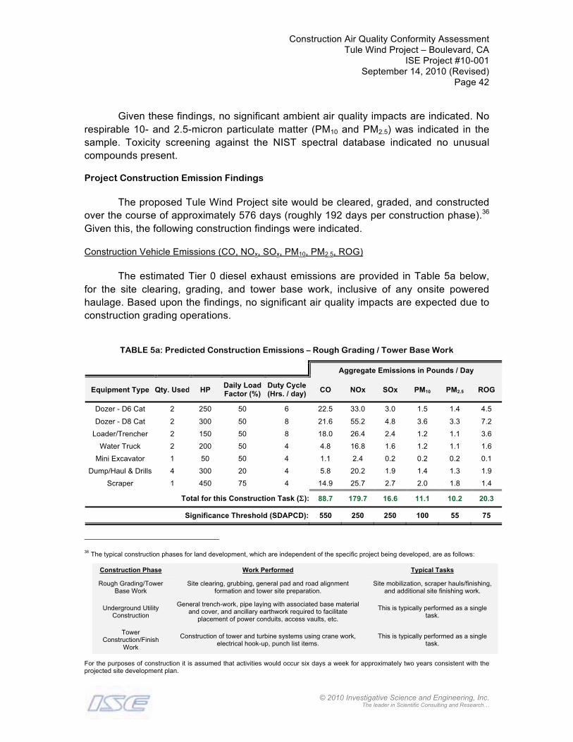
The proposed Tule Wind Project site would be cleared, graded, and constructed over the course of approximately 576 days (roughly 192 days per construction phase).36
Given this, the following construction findings were indicated.
Construction Vehicle Emissions (CO, NOx, SOx, PM10, PM2.5, ROG)
The estimated Tier 0 diesel exhaust emissions are provided in Table 5a below,for the site clearing, grading, and tower base work, inclusive of any onsite powered haulage. Based upon the findings, no significant air quality impacts are expected due to construction grading operations.
TABLE 5a: Predicted Construction Emissions – Rough Grading / Tower Base Work
Aggregate Emissions in Pounds / Day
Equipment Type Qty. Used HP Daily Load Factor (%)
Duty Cycle (Hrs. / day) CO NOx SOx PM10 PM2.5 ROG
Dozer - D6 Cat 2 250 50 6 22.5 33.0 3.0 1.5 1.4 4.5
Dozer - D8 Cat 2 300 50 8 21.6 55.2 4.8 3.6 3.3 7.2
Loader/Trencher 2 150 50 8 18.0 26.4 2.4 1.2 1.1 3.6
Water Truck 2 200 50 4 4.8 16.8 1.6 1.2 1.1 1.6
Mini Excavator 1 50 50 4 1.1 2.4 0.2 0.2 0.2 0.1
Dump/Haul & Drills 4 300 20 4 5.8 20.2 1.9 1.4 1.3 1.9
Scraper 1 450 75 4 14.9 25.7 2.7 2.0 1.8 1.4
Total for this Construction Task (ΣΣ): 88.7 179.7 16.6 11.1 10.2 20.3
Significance Threshold (SDAPCD): 550 250 250 100 55 75
36 The typical construction phases for land development, which are independent of the specific project being developed, are as follows:
Construction Phase Work Performed Typical Tasks
Rough Grading/Tower Base Work
Site clearing, grubbing, general pad and road alignment formation and tower site preparation.
Site mobilization, scraper hauls/finishing, and additional site finishing work.
Underground Utility Construction
General trench-work, pipe laying with associated base material and cover, and ancillary earthwork required to facilitate
placement of power conduits, access vaults, etc.
This is typically performed as a single task.
Tower Construction/Finish
Work
Construction of tower and turbine systems using crane work, electrical hook-up, punch list items.
This is typically performed as a single task.
For the purposes of construction it is assumed that activities would occur six days a week for approximately two years consistent with the projected site development plan.
Construction Air Quality Conformity AssessmentTule Wind Project – Boulevard, CA
ISE Project #10-001September 14, 2010 (Revised)
Page 43
© 2010 Investigative Science and Engineering, Inc. The leader in Scientific Consulting and Research…
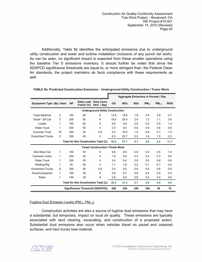
Additionally, Table 5b identifies the anticipated emissions due to underground utility construction and tower and turbine installation (inclusive of any punch list work). As can be seen, no significant impact is expected from these smaller operations using the baseline Tier 0 emissions inventory. It should further be noted that since the SDAPCD significance thresholds are equal to, or more stringent than, the Federal CleanAir standards, the project maintains de facto compliance with these requirements as well.
TABLE 5b: Predicted Construction Emissions – Underground Utility Construction / Tower Work
Aggregate Emissions in Pounds / Day
Equipment Type Qty. Used HP Daily LoadFactor (%)
Duty Cycle (Hrs. / day) CO NOx SOx PM10 PM2.5 ROG
Underground Utility Construction
Track Backhoe 2 150 50 6 13.5 19.8 1.8 0.9 0.8 2.7Dozer - D4 Cat 2 200 50 6 18.0 26.4 2.4 1.2 1.1 3.6
Loader 1 150 50 6 6.8 9.9 0.9 0.5 0.5 1.4Water Truck 1 200 50 4 2.4 8.4 0.8 0.6 0.6 0.8
Concrete Truck 16 250 25 0.5 3.0 10.5 1.0 0.8 0.7 1.0Dump/Haul Trucks 2 300 45 4 6.5 22.7 2.2 1.6 1.5 2.2
Total for this Construction Task (ΣΣ): 50.2 97.7 9.1 5.6 5.2 11.7
Tower Construction / Finish Work
Skid Steer Cat 1 150 50 6 6.8 9.9 0.9 0.5 0.5 1.4Hydraulic Crane 1 200 25 4 1.8 4.6 0.4 0.3 0.3 0.6
Water Truck 1 200 50 4 2.4 8.4 0.8 0.6 0.6 0.8Welding Rig 1 50 50 4 1.1 1.8 0.2 0.1 0.1 0.2
Dump/Haul Trucks 6 300 45 0.5 2.4 8.5 0.8 0.6 0.6 0.8Paver/Compactor 1 150 35 8 2.9 9.7 0.8 0.4 0.4 0.4
Roller 1 150 35 8 2.9 8.4 0.8 0.4 0.4 0.8
Total for this Construction Task (ΣΣ): 20.3 51.3 4.7 2.9 2.9 5.0
Significance Threshold (SDAPCD): 550 250 250 100 55 75
Fugitive Dust Emission Levels (PM10, PM2.5)
Construction activities are also a source of fugitive dust emissions that may have a substantial, but temporary, impact on local air quality. These emissions are typically associated with land clearing, excavating, and construction of a proposed action. Substantial dust emissions also occur when vehicles travel on paved and unpaved surfaces, and haul trucks lose material.

Construction Air Quality Conformity AssessmentTule Wind Project – Boulevard, CA
ISE Project #10-001September 14, 2010 (Revised)
Page 44
© 2010 Investigative Science and Engineering, Inc. The leader in Scientific Consulting and Research…
Dust emissions and impacts vary substantially from day to day, depending on the level of activity, the specific operation being conducted, and the prevailing meteorological conditions. Wet dust suppression techniques, such as watering and/or applying chemical stabilization, would be used during construction to suppress the fine dust particulates from leaving the ground surface and becoming airborne through the action of mechanical disturbance or wind motion.
Construction grading operations at the proposed Tule Wind Project development site are anticipated as being approximately 2,550,000 cubic-yards (cy) of material moved over an anticipated 576-day earthwork period.37
For alluvium-type material, the project earthwork would have a total working
weight of,
Working Weight = 2,550,000 cubic yards ×1.3 tons
cubic yard= 3,315,000 tons
Out of the total quantity identified above, it is estimated that roughly 50-percent of the working weight would be capable of generating PM10 due to the initial geologic findings of hard rock and minimal topsoil. Thus, for the purposes of analysis, the working weight of earthwork material capable of generating some amount of PM10 would be 1,657,500.0 tons. Thus, the average mass grading earthwork movement per day would be 2,877.6 tons/day.
Following the analysis procedure identified in the SCAQMD CEQA Handbook for PM10 emissions from fugitive dust gives the following semi-empirical relationship for aggregate respirable dust generation,
PM10 = 0.00112 ×
WS5
⎛⎝⎜
⎞⎠⎟
1.3
SMC2
⎛⎝⎜
⎞⎠⎟
1.4
⎡
⎣
⎢⎢⎢⎢
⎤
⎦
⎥⎥⎥⎥
× ET
where, PM10 = Fugitive dust emissions in pounds,WS = Ambient wind speed,SMC = Surface Moisture Content, generally defined as the weight of the water (Ww) divided by the
weight of the soil (Ws) as measured at the surface in grams per gram.ET = Earthwork Tonnage moved per day,
37 This is based upon the following project-estimated grading areas to an average depth of three-feet: 134 wind turbine pads = 134 acres, access roads and improvements = 58.3 acres, substation pad formation = 5 acres, operations and maintenance area = 5 acres, batch plant area = 5 acres, parking lot area = 10 acres, 19 lay down areas = 48 acres.

Construction Air Quality Conformity AssessmentTule Wind Project – Boulevard, CA
ISE Project #10-001September 14, 2010 (Revised)
Page 45
© 2010 Investigative Science and Engineering, Inc. The leader in Scientific Consulting and Research…
Substituting a minimum SMC value of 0.25 (which is extremely conservative for
an ambient dirt/sand condition), and a maximum credible wind speed scenario of 12 MPH (WS = 12), gives the following result,
PM10 = 0.00112 ×
125
⎛⎝⎜
⎞⎠⎟
1.3
0.252
⎛⎝⎜
⎞⎠⎟
1.4
⎡
⎣
⎢⎢⎢⎢
⎤
⎦
⎥⎥⎥⎥
× 2,877.6 = 184.7
or, a level of 184.7 pounds of PM10 generated per day. It should be noted that surface wetting will be utilized during all phases of earthwork operations at a minimum level of three times per day for a maximum control efficiency of 68% per the SCAQMDmethodology. Thus, the final wetted PM10 level would be,
PM10 = 1− 0.6( ) ×184.7 = 59.1
or a total fugitive dust generated load of 59.1 pounds per day. This level is far below the 100 pounds per day threshold established by the SDAPCD and the Federal CAA thresholds. Therefore, no impacts are expected from this phase of construction. The commensurate PM2.5 level would be 12.3 pounds per day, which is also below the proposed State threshold of significance of 55 pounds per day for this pollutant and below the Federal CAA threshold.
Finally, unpaved road travel due to construction activities is also unknown at this time. For the purposes of analysis, it will be assumed that contractors’ vehicles moving onsite would traverse a total of 100 miles per day (VMT) during the earthwork and site preparation phases.
Substituting the applicable project values of VMT = 100, SLP = 6.0 (sand/gravel road with watering), MVS = 5 miles per hour, MVW = 4 tons (average gross vehicular weight), NW = 6 wheels (average number of wheels), and RD38 = 44.0 (rain days), gives the following result,
PM10 = 100.0 × 2.16
12⎛⎝⎜
⎞⎠⎟
530
⎛⎝⎜
⎞⎠⎟
43
⎛⎝⎜
⎞⎠⎟
0.7 64
⎛⎝⎜
⎞⎠⎟
0.5 365 − 44365
⎛⎝⎜
⎞⎠⎟
⎡
⎣⎢⎢
⎤
⎦⎥⎥= 23.1
or, a level of approximately 23.1 pounds of PM10 generated per day. This activity alone would not generate a significant impact under SDAPCD standards. The
38 Based upon U.S. Weather Service average precipitation year data for San Diego County.
Construction Air Quality Conformity AssessmentTule Wind Project – Boulevard, CA
ISE Project #10-001September 14, 2010 (Revised)
Page 46
© 2010 Investigative Science and Engineering, Inc. The leader in Scientific Consulting and Research…
commensurate PM2.5 level would be 4.9 pounds per day, which is also below the proposed State threshold of significance identified above as well as below the Federal CAA threshold.
Combustion-Fired Health-Risk Emission Levels (PM10, PM2.5)
Onsite construction equipment was found to generate worst-case daily pollutant levels during the rough grading phase. These emissions are assumed to occur over any given 24-hour day (thereby providing an upper bound on expected emission concentrations) and direct comparison with NAAQS and CAAQS standards.
Although all stable criteria pollutants are provided, it should be noted that for cancer-risk potential, only combustion-fired PM10 particulates are considered with PM2.5
concentrations being determined through the aforementioned fractional emission estimates. This methodology essentially applies all of the diesel emissions over this working area and provides a worst-case assessment of the impacts to sensitive receptors.
The proposed Tule Wind Project site has a maximum project footprint of roughly 1,067,220,000 square-feet (99,147,825 m2), based upon data obtained from the project site plans.39 The aggregate Tier 0 mitigated emission rates for the various criteria pollutants, in grams per second, and grams per square-meter (m2) per second, areshown in Table 6 on the following page.40 The expected combustion-fired construction emission concentrations from the SCREEN3 modeling are shown in Table 7. The output model results are provided as an attachment to this report.
Based upon the model results, all criteria pollutants were below the recommended health risk level with a PM10 risk probability of 0.005% per 70-year exposure duration, assuming the implementation of T-BACT. Given this, no significant carcinogenic impact potential is expected due to proposed grading operations.
39 As determined to consist of the worst-case polygon enclosing the turbine locations and access roads shown in Figure 3 of this report.40 As a required input parameter for the SCREEN3 model.

Construction Air Quality Conformity AssessmentTule Wind Project – Boulevard, CA
ISE Project #10-001September 14, 2010 (Revised)
Page 47
© 2010 Investigative Science and Engineering, Inc. The leader in Scientific Consulting and Research…
TABLE 6: Predicted Onsite Diesel-Fired Construction Emission Rates (Tier 0)
Criteria Pollutant Max Daily Emissions (pounds)
Daily Site Emission Rates (grams/second)
Average Area Emission Rates (grams/m2/second)
CO 88.7 0.4657 4.6967E-09
NOx 179.7 0.9434 9.5151E-09
SOx 16.6 0.0871 8.7897E-10
PM10 11.1 0.0583 5.8775E-10
PM2.5 10.2 0.0535 5.4009E-10
Total averaging time is 24 hours x 60 minutes/hour x 60 seconds/minute = 86,400 seconds per CAAQS standards.
The area emission rates are shown in scientific notation and are expressed in the form of mantissa-exponent to base 10.
One pound-mass = 453.592 grams.
TABLE 7: SCREEN3 Predicted Diesel-Fired Emission Concentrations
Criteria PollutantPollutant
Concentration (µg/m3)
Pollutant Concentration
(ppm)
Pollutant Risk Probability (percent risk per person for
70-year exposure)Significant?
CO 1.46 0.0013 n/a No
NOx 2.96 0.0016 n/a No
SOx 0.27 0.0001 n/a No
PM10 0.18 - - 0.005% No
PM2.5 0.17 - - n/a No
Diesel risk calculation based upon ARB 1999 Staff Report from the Scientific Review Panel (SRP) on Diesel Toxics inhaled in a 70-year lifetime.Conversion Factors (approximate):
CO: 1 ppm = 1,150 µg/m3 @ 25 deg-C STP, NOx: 1 ppm = 1,880 µg/m3 @ 25 deg-C STPSOx: 1 ppm = 2,620 µg/m3 @ 25 deg-C STP, PM10 and PM2.5: 1 ppm = 1 g/m3 (solid)
PM2.5 levels based upon the CEIDARS database fractional emission factor for diesel construction equipment of 0.920 PM2.5 / PM10.
Additionally, the analysis identified a worst-case PM10 level of 0.18 µg/m3
occurring at a distance of 7,042 meters (23,098 feet) from the project site. This pollutant concentration is far below both the NAAQS and CAAQS thresholds as previously shown in Figure 5 for any given exposure period. This predicted diesel-fired PM10 dispersion pattern as a function of distance from the site can be seen in Figure 10 on the following page. No cumulative contribution from the site would be physically possible beyond the extents identified in this figure.41
41 Which, assuming a theoretical Gaussian distribution, would yield an effective no impact distance of 92,392 feet (or 17.50 miles).

Construction Air Quality Conformity AssessmentTule Wind Project – Boulevard, CA
ISE Project #10-001September 14, 2010 (Revised)
Page 48
© 2010 Investigative Science and Engineering, Inc. The leader in Scientific Consulting and Research…
FIGURE 10: Predicted Combustion-Fired Diesel PM10 Dispersion Pattern (ISE 9/10)
Finally, anticipated diesel-fired PM2.5 levels would not be expected to exceed 0.20 µg/m3, which is also below the Federal NAAQS 24-hour threshold of 35 µg/m3
(there are no State thresholds for this pollutant). No cumulative contribution of PM2.5
from the site would be physically possible due to the reasons cited above.
Odor Impact Potential from Proposed Site
The inhalation of volatile organic compounds (VOC’s) causes smell sensations in humans. These odors can affect human health in four primary ways:
o The VOC’s can produce toxicological effects; o The odorant compounds can cause irritations in the eye, nose, and throat; o The VOC’s can stimulate sensory nerves that can cause potentially harmful health
effects; o The exposure to perceived unpleasant odors can stimulate negative cognitive and
emotional responses based on previous experiences with such odors.
0
0.02
0.04
0.06
0.08
0.1
0.12
0.14
0.16
0.18
0.2
Con
cent
ratio
n in
mic
rogr
ams
per C
ubic
Met
er
Distance From Emission Source (ft)
Down Wind Dispersion
Pattern
Construction Air Quality Conformity AssessmentTule Wind Project – Boulevard, CA
ISE Project #10-001September 14, 2010 (Revised)
Page 49
© 2010 Investigative Science and Engineering, Inc. The leader in Scientific Consulting and Research…
Development of the proposed project site could generate trace amounts (less than 1 µg/m3) of substances such as ammonia, carbon dioxide, hydrogen sulfide, methane, dust, organic dust, and endotoxins (i.e., bacteria are present in the dust). Additionally, proposed onsite uses could generate such substances as volatile organic acids, alcohols, aldehydes, amines, fixed gases, carbonyls, esters, sulfides, disulfides, mercaptans, and nitrogen heterocycles.
It should be noted that odor generation impacts due to the project are not expected to be significant, since any odor generation would be intermittent and would terminate upon completion of the construction phase of the project, if it occurred at all. As a result, no significant air quality impacts are expected to surrounding residential receptors. No mitigation for odors is identified. Construction Worker Vehicular Emission Levels
The Tule Wind Project site is expected to have a worst-case construction trip generation level of 1,250 ADT based upon the cumulative trip generation produced for the proposed project.42,43 The average one-way trip length would be 30.0 miles given the expected service increment of the proposed facility.44 A median speed of 45 MPH was used, consistent with average values observed (i.e., combined highway and surface street traffic activity).
The calculated daily emission levels due to travel to and from the site are shown in Table 8 on the following page for the aggregate project trip generation. Based upon the findings, no significant impacts for any criteria pollutants were identified.
Predicted CO / NOx / PM10 / PM2.5 Concentration Levels
Table 9, on Page 51 of this report, lists the roadway segments identified by the traffic engineer for the cumulative build out plus project scenario, the predicted peak hour traffic volume, and the expected CO, NOx, PM10, and PM2.5 emissions at 100 feet from the road centerline (minimum possible standing receptor distance). Based upon the dispersion model findings, no localized criteria pollutant impacts were identified for any roadway segment examined. The roadway segments examined were found to comply with the CAAQS and NAAQS standards.
42 Source: Full Traffic Impact Study – Tule Wind Farm, LLG, Inc., 3/26/10.43 Motor vehicles are the primary source of emissions associated with the proposed project area. Typically, uses such as the proposed project do not directly emit significant amounts of air pollutants from onsite activities. Rather, vehicular trips to and from these land uses are the significant contributor. Further, it should be additionally noted that including construction worker trips provides a worst-case upper bound estimate on project emissions, since worker trips are typically already accounted for in General Plan traffic estimates and would have been the subject of other air quality assessments (such as for the workers’ housing). To avoid double counting of emissions, only the additional travel increment is factored into the analysis.44 The average assumed trip length is the average travel distance to or from the site. It is anticipated that some end trips will be shorter, and some longer, but for the purposes of analysis, the average value is given.
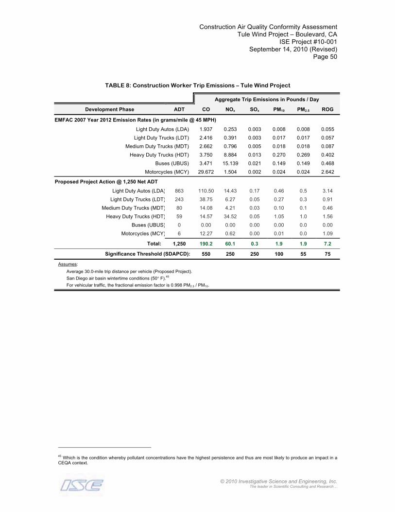
Construction Air Quality Conformity AssessmentTule Wind Project – Boulevard, CA
ISE Project #10-001September 14, 2010 (Revised)
Page 50
© 2010 Investigative Science and Engineering, Inc. The leader in Scientific Consulting and Research…
TABLE 8: Construction Worker Trip Emissions – Tule Wind Project
Aggregate Trip Emissions in Pounds / Day
Development Phase ADT CO NOx SOx PM10 PM2.5 ROG
EMFAC 2007 Year 2012 Emission Rates (in grams/mile @ 45 MPH)
Light Duty Autos (LDA) 1.937 0.253 0.003 0.008 0.008 0.055
Light Duty Trucks (LDT) 2.416 0.391 0.003 0.017 0.017 0.057
Medium Duty Trucks (MDT) 2.662 0.796 0.005 0.018 0.018 0.087
Heavy Duty Trucks (HDT) 3.750 8.884 0.013 0.270 0.269 0.402
Buses (UBUS) 3.471 15.139 0.021 0.149 0.149 0.468
Motorcycles (MCY) 29.672 1.504 0.002 0.024 0.024 2.642
Proposed Project Action @ 1,250 Net ADT
Light Duty Autos (LDA) 863 110.50 14.43 0.17 0.46 0.5 3.14
Light Duty Trucks (LDT) 243 38.75 6.27 0.05 0.27 0.3 0.91
Medium Duty Trucks (MDT) 80 14.08 4.21 0.03 0.10 0.1 0.46
Heavy Duty Trucks (HDT) 59 14.57 34.52 0.05 1.05 1.0 1.56
Buses (UBUS) 0 0.00 0.00 0.00 0.00 0.0 0.00
Motorcycles (MCY) 6 12.27 0.62 0.00 0.01 0.0 1.09
Total: 1,250 190.2 60.1 0.3 1.9 1.9 7.2
Significance Threshold (SDAPCD): 550 250 250 100 55 75
Assumes:Average 30.0-mile trip distance per vehicle (Proposed Project).San Diego air basin wintertime conditions (50° F).45
For vehicular traffic, the fractional emission factor is 0.998 PM2.5 / PM10.
45 Which is the condition whereby pollutant concentrations have the highest persistence and thus are most likely to produce an impact in a CEQA context.

Construction Air Quality Conformity AssessmentTule Wind Project – Boulevard, CA
ISE Project #10-001September 14, 2010 (Revised)
Page 51
© 2010 Investigative Science and Engineering, Inc. The leader in Scientific Consulting and Research…
TABLE 9: Roadway Segment Incremental Project Increases for CO, NOX, PM10 and PM2.5
Roadway Segment LOS ADT ∆ CO (ppm) ∆ NOX (pphm) ∆ PM10 (ppm) ∆ PM2.5 (ppm)
EXISTING BASELINE CONDITIONS
Crestwood Road North of I-8 A 1,060 0.0 0.5 0.4 0.4
Ribbonwood Road North of I-8 A 270 0.0 0.4 0.2 0.2I-8 to Old Highway 80 A 1,230 0.0 0.6 0.4 0.4
McCain Valley Road North of Old Highway 80 A 110 0.0 0.4 0.2 0.2
Old Highway 80 Ribbonwood Road to McCain Valley Road A 990 0.0 0.5 0.4 0.4
EXISTING + PROJECT CONDITONS
Crestwood Road North of I-8 A 1,810 0.0 0.6 0.5 0.5
Ribbonwood Road North of I-8 A 645 0.0 0.5 0.3 0.3I-8 to Old Highway 80 A 1,355 0.0 0.6 0.4 0.4
McCain Valley Road North of Old Highway 80 A 235 0.0 0.4 0.2 0.2
Old Highway 80 Ribbonwood Road to McCain Valley Road A 1,115 0.0 0.5 0.4 0.4
EXISTING + PROJECT + CUMULATIVE CONDITIONS
Crestwood Road North of I-8 B 3,140 0.1 0.7 0.6 0.6
Ribbonwood Road North of I-8 A 985 0.0 0.5 0.4 0.4I-8 to Old Highway 80 B 2,895 0.1 0.7 0.6 0.6
McCain Valley Road North of Old Highway 80 A 375 0.0 0.4 0.2 0.2
Old Highway 80 Ribbonwood Road to McCain Valley Road B 2,355 0.0 0.7 0.5 0.5

Construction Air Quality Conformity AssessmentTule Wind Project – Boulevard, CA
ISE Project #10-001September 14, 2010 (Revised)
Page 52
© 2010 Investigative Science and Engineering, Inc. The leader in Scientific Consulting and Research…
CONCLUSIONS AND RECOMMENDATIONS
Aggregate Project Emissions
The aggregate emission levels produced by the proposed Tule Wind Project development plan are shown in Table 10 below. Based upon the findings, no construction air quality impacts are anticipated.
TABLE 10: Aggregate Construction Emissions Synopsis – Tule Wind Project
Aggregate Emissions in Pounds / Day
CONSTRUCTION SCENARIO EXAMINED CO NOx SOx PM10 PM2.546 ROG /
VOC
Grading Emissions (Tier 0 Baseline): 88.7 179.7 16.6 11.1 10.2 20.3
Surface Grading Dust Generation: - - - - - - 59.1 12.3 - -
Powered Haulage Dust Generation: 0.0 0.0 0.0 23.1 4.9 0.0
Construction Vehicular Traffic Generation: 190.2 60.1 0.3 1.9 1.9 7.2
Total (ΣΣ): 278.9 239.8 16.9 95.2 29.3 27.5
Significance Threshold (SDAPCD): 550 250 250 100 55 75
The Tule Wind Project would be required to obtain from the San Diego Air Pollution Control District (SDAPCD) the following permits:
1. Temporary batch plant: Permit to Construct, Permit to Operate2. Transmission Substation: Permit to Construct, Permit to Operate
These permits would not be required as part of the CEQA/NEPA process, but would be needed prior to obtaining permits to construct and operate the above citedfacilities. Additional emission review, specific to these uses, would be required with the permit applications.
Consistency with Regional Air Quality Management Plans
Finally, the San Diego APCD establishes what could be thought of as an “emissions budget” or Regional Air Quality Strategy (RAQS) for the San Diego Air Basin. This budget takes into account existing conditions, planned growth based on General Plans for cities within the region, and air quality control measures implemented by the SDAPCD per the requirements of the Federal CAA. The “emissions budget” accounts for current emissions associated with the proposed project, as well as previously approved 46 Values shown in this column are for informational purposes only. PM2.5 emissions are not currently regulated by CARB. The 55 pound-per-day level shown is a proposed standard that has not been adopted.

Construction Air Quality Conformity AssessmentTule Wind Project – Boulevard, CA
ISE Project #10-001September 14, 2010 (Revised)
Page 53
© 2010 Investigative Science and Engineering, Inc. The leader in Scientific Consulting and Research…
projects consistent with current General Plan policies (commonly known as the Consistency Criterion of the RAQS).
The proposed Tule Wind Project development is consistent with future build out plans for the project site under the County’s General Plan, being less impactive than the current housing densities projected, and therefore satisfies the Consistency Criterion of the RAQS. CERTIFICATION OF ACCURACY AND QUALIFICATIONS
This report was prepared by Investigative Science and Engineering, Inc. (ISE), located at 1134 D Street, Ramona, CA 92065. The members of its professional staff contributing to the report are listed below:
Rick Tavares Ph.D. Civil Engineering([email protected]) M.S. Structural Engineering
M.S. Mechanical EngineeringB.S. Aerospace Engineering / Engineering Mechanics
Karen Tavares B.S. Electrical Engineering([email protected])
ISE affirms to the best of its knowledge and belief that the statements and information contained herein are in all respects true and correct as of the date of this report. Should the reader have any questions regarding the findings and conclusions presented in this report, please do not hesitate to contact ISE at (760) 787-0016.
Content and information contained within this report is intended only for the subject project and is protected under 17 U.S.C. §§ 101 through 810. Original reports contain a non-photo blue ISE watermark at the bottom of each page.
Approved as to Form and Content:
Rick Tavares, Ph.D.
Project PrincipalInvestigative Science and Engineering, Inc. (ISE)
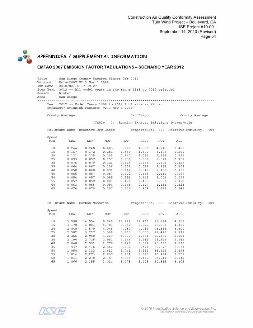
Construction Air Quality Conformity AssessmentTule Wind Project – Boulevard, CA
ISE Project #10-001September 14, 2010 (Revised)
Page 54
© 2010 Investigative Science and Engineering, Inc. The leader in Scientific Consulting and Research…
APPENDICES / SUPPLEMENTAL INFORMATION
EMFAC 2007 EMISSION FACTOR TABULATIONS – SCENARIO YEAR 2012
Title : San Diego County Subarea Winter CYr 2012Version : Emfac2007 V2.3 Nov 1 2006Run Date : 2010/02/16 17:39:27Scen Year: 2012 -- All model years in the range 1968 to 2012 selectedSeason : WinterArea : San Diego***************************************************************************************** Year: 2012 -- Model Years 1968 to 2012 Inclusive -- Winter Emfac2007 Emission Factors: V2.3 Nov 1 2006
County Average San Diego County Average
Table 1: Running Exhaust Emissions (grams/mile)
Pollutant Name: Reactive Org Gases Temperature: 50F Relative Humidity: 40%
Speed MPH LDA LDT MDT HDT UBUS MCY ALL
10 0.244 0.248 0.405 3.008 1.936 4.215 0.410 15 0.167 0.172 0.281 1.589 1.409 3.405 0.269 20 0.121 0.125 0.205 0.947 1.066 2.888 0.191 25 0.093 0.097 0.157 0.758 0.839 2.571 0.151 30 0.075 0.079 0.126 0.615 0.685 2.405 0.125 35 0.064 0.067 0.106 0.512 0.582 2.363 0.109 40 0.058 0.060 0.094 0.442 0.512 2.438 0.100 45 0.055 0.057 0.087 0.402 0.468 2.642 0.097 50 0.054 0.057 0.085 0.391 0.445 3.004 0.099 55 0.057 0.059 0.087 0.406 0.438 3.583 0.108 60 0.063 0.065 0.094 0.448 0.447 4.481 0.123 65 0.074 0.076 0.107 0.516 0.474 5.873 0.149
Pollutant Name: Carbon Monoxide Temperature: 50F Relative Humidity: 40%
Speed MPH LDA LDT MDT HDT UBUS MCY ALL
10 3.598 4.554 5.645 13.849 14.475 29.624 4.815 15 3.178 4.001 4.703 9.760 9.927 25.803 4.109 20 2.848 3.570 4.045 7.282 7.214 23.516 3.600 25 2.582 3.227 3.569 5.915 5.555 22.418 3.231 30 2.366 2.950 3.219 4.977 4.531 22.369 2.951 35 2.190 2.728 2.961 4.345 3.915 23.393 2.742 40 2.048 2.551 2.779 3.947 3.582 25.686 2.596 45 1.937 2.416 2.662 3.750 3.471 29.672 2.511 50 1.858 2.322 2.612 3.741 3.562 36.126 2.493 55 1.814 2.273 2.637 3.931 3.870 46.424 2.559 60 1.811 2.278 2.757 4.354 4.452 63.014 2.742 65 1.866 2.355 3.014 5.078 5.423 90.365 3.105

Construction Air Quality Conformity AssessmentTule Wind Project – Boulevard, CA
ISE Project #10-001September 14, 2010 (Revised)
Page 55
© 2010 Investigative Science and Engineering, Inc. The leader in Scientific Consulting and Research…
Pollutant Name: Oxides of Nitrogen Temperature: 50F Relative Humidity: 40%
Speed MPH LDA LDT MDT HDT UBUS MCY ALL
10 0.391 0.616 1.095 15.228 23.752 1.320 1.162 15 0.348 0.542 0.973 11.723 19.230 1.321 0.960 20 0.316 0.488 0.888 10.139 16.369 1.333 0.851 25 0.292 0.448 0.831 9.557 14.638 1.353 0.795 30 0.274 0.420 0.795 9.148 13.742 1.381 0.756 35 0.263 0.402 0.779 8.899 13.534 1.415 0.733 40 0.256 0.392 0.779 8.809 13.978 1.456 0.724 45 0.253 0.391 0.796 8.884 15.139 1.504 0.729 50 0.255 0.397 0.833 9.140 17.200 1.558 0.750 55 0.262 0.411 0.891 9.610 20.512 1.618 0.788 60 0.273 0.435 0.977 10.343 25.694 1.687 0.848 65 0.290 0.471 1.102 11.419 33.832 1.765 0.938
Pollutant Name: Sulfur Dioxide Temperature: 50F Relative Humidity: 40%
Speed MPH LDA LDT MDT HDT UBUS MCY ALL
10 0.007 0.009 0.012 0.022 0.024 0.003 0.009 15 0.005 0.007 0.009 0.019 0.023 0.002 0.007 20 0.004 0.006 0.008 0.016 0.022 0.002 0.006 25 0.004 0.005 0.006 0.015 0.022 0.002 0.005 30 0.003 0.004 0.006 0.015 0.022 0.002 0.004 35 0.003 0.004 0.005 0.014 0.022 0.002 0.004 40 0.003 0.004 0.005 0.014 0.021 0.002 0.004 45 0.003 0.003 0.005 0.013 0.021 0.002 0.004 50 0.003 0.004 0.005 0.013 0.021 0.002 0.004 55 0.003 0.004 0.005 0.013 0.022 0.002 0.004 60 0.003 0.004 0.006 0.014 0.022 0.003 0.004 65 0.004 0.005 0.006 0.014 0.022 0.003 0.005
Pollutant Name: PM10 Temperature: 50F Relative Humidity: 40%
Speed MPH LDA LDT MDT HDT UBUS MCY ALL
10 0.038 0.079 0.082 0.793 0.534 0.036 0.087 15 0.026 0.055 0.057 0.560 0.400 0.030 0.060 20 0.019 0.040 0.042 0.420 0.311 0.026 0.044 25 0.014 0.030 0.032 0.357 0.250 0.023 0.035 30 0.012 0.024 0.026 0.312 0.209 0.022 0.030 35 0.010 0.021 0.022 0.284 0.180 0.022 0.026 40 0.009 0.018 0.020 0.270 0.161 0.023 0.024 45 0.008 0.017 0.018 0.270 0.149 0.024 0.023 50 0.008 0.017 0.018 0.285 0.143 0.028 0.023 55 0.008 0.018 0.019 0.313 0.142 0.033 0.025 60 0.009 0.019 0.020 0.354 0.146 0.041 0.028 65 0.011 0.022 0.023 0.409 0.156 0.053 0.032
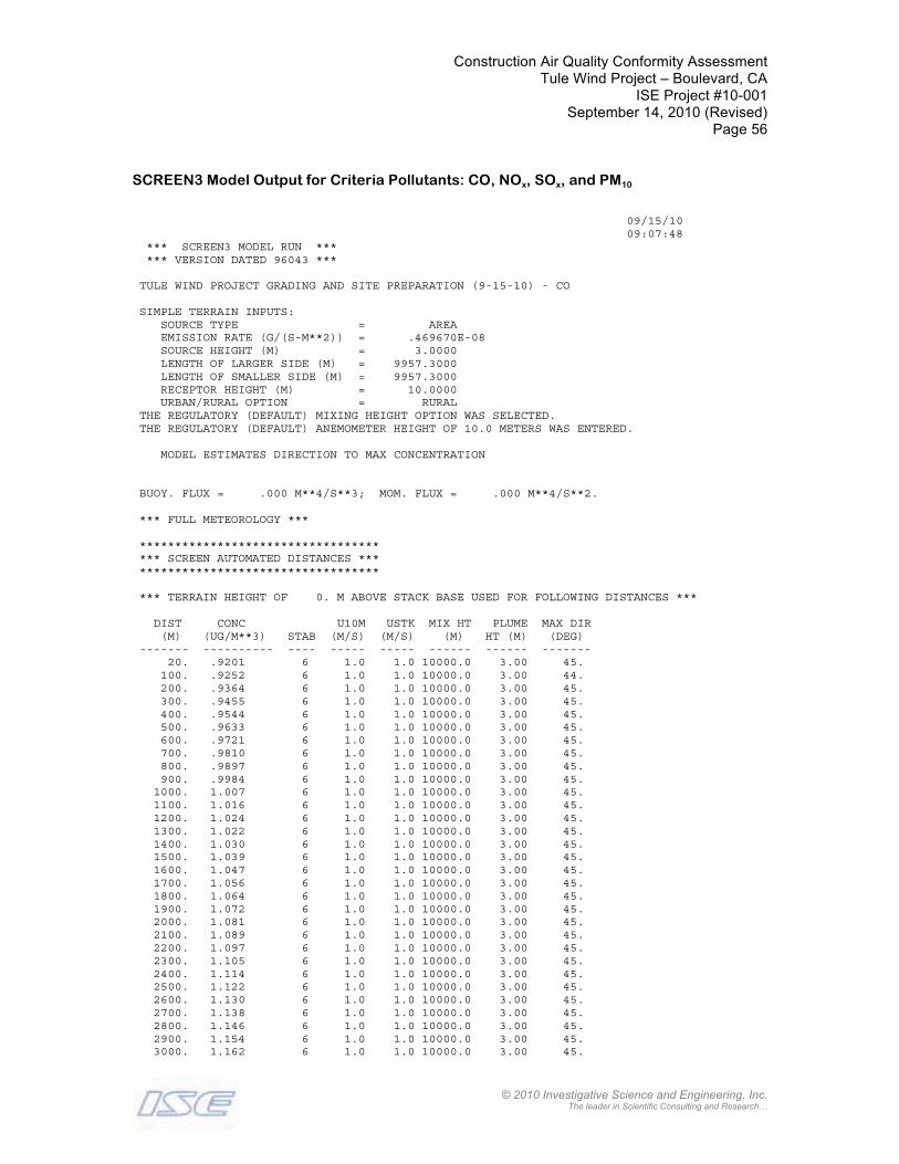
Construction Air Quality Conformity AssessmentTule Wind Project – Boulevard, CA
ISE Project #10-001September 14, 2010 (Revised)
Page 56
© 2010 Investigative Science and Engineering, Inc. The leader in Scientific Consulting and Research…
SCREEN3 Model Output for Criteria Pollutants: CO, NOx, SOx, and PM10
09/15/10 09:07:48 *** SCREEN3 MODEL RUN *** *** VERSION DATED 96043 ***
TULE WIND PROJECT GRADING AND SITE PREPARATION (9-15-10) - CO
SIMPLE TERRAIN INPUTS: SOURCE TYPE = AREA EMISSION RATE (G/(S-M**2)) = .469670E-08 SOURCE HEIGHT (M) = 3.0000 LENGTH OF LARGER SIDE (M) = 9957.3000 LENGTH OF SMALLER SIDE (M) = 9957.3000 RECEPTOR HEIGHT (M) = 10.0000 URBAN/RURAL OPTION = RURAL THE REGULATORY (DEFAULT) MIXING HEIGHT OPTION WAS SELECTED. THE REGULATORY (DEFAULT) ANEMOMETER HEIGHT OF 10.0 METERS WAS ENTERED.
MODEL ESTIMATES DIRECTION TO MAX CONCENTRATION
BUOY. FLUX = .000 M**4/S**3; MOM. FLUX = .000 M**4/S**2.
*** FULL METEOROLOGY ***
********************************** *** SCREEN AUTOMATED DISTANCES *** **********************************
*** TERRAIN HEIGHT OF 0. M ABOVE STACK BASE USED FOR FOLLOWING DISTANCES ***
DIST CONC U10M USTK MIX HT PLUME MAX DIR (M) (UG/M**3) STAB (M/S) (M/S) (M) HT (M) (DEG)------- ---------- ---- ----- ----- ------ ------ -------
20. .9201 6 1.0 1.0 10000.0 3.00 45. 100. .9252 6 1.0 1.0 10000.0 3.00 44. 200. .9364 6 1.0 1.0 10000.0 3.00 45. 300. .9455 6 1.0 1.0 10000.0 3.00 45. 400. .9544 6 1.0 1.0 10000.0 3.00 45. 500. .9633 6 1.0 1.0 10000.0 3.00 45. 600. .9721 6 1.0 1.0 10000.0 3.00 45. 700. .9810 6 1.0 1.0 10000.0 3.00 45. 800. .9897 6 1.0 1.0 10000.0 3.00 45. 900. .9984 6 1.0 1.0 10000.0 3.00 45. 1000. 1.007 6 1.0 1.0 10000.0 3.00 45. 1100. 1.016 6 1.0 1.0 10000.0 3.00 45. 1200. 1.024 6 1.0 1.0 10000.0 3.00 45. 1300. 1.022 6 1.0 1.0 10000.0 3.00 45. 1400. 1.030 6 1.0 1.0 10000.0 3.00 45. 1500. 1.039 6 1.0 1.0 10000.0 3.00 45. 1600. 1.047 6 1.0 1.0 10000.0 3.00 45. 1700. 1.056 6 1.0 1.0 10000.0 3.00 45. 1800. 1.064 6 1.0 1.0 10000.0 3.00 45. 1900. 1.072 6 1.0 1.0 10000.0 3.00 45. 2000. 1.081 6 1.0 1.0 10000.0 3.00 45. 2100. 1.089 6 1.0 1.0 10000.0 3.00 45. 2200. 1.097 6 1.0 1.0 10000.0 3.00 45. 2300. 1.105 6 1.0 1.0 10000.0 3.00 45. 2400. 1.114 6 1.0 1.0 10000.0 3.00 45. 2500. 1.122 6 1.0 1.0 10000.0 3.00 45. 2600. 1.130 6 1.0 1.0 10000.0 3.00 45. 2700. 1.138 6 1.0 1.0 10000.0 3.00 45. 2800. 1.146 6 1.0 1.0 10000.0 3.00 45. 2900. 1.154 6 1.0 1.0 10000.0 3.00 45. 3000. 1.162 6 1.0 1.0 10000.0 3.00 45.
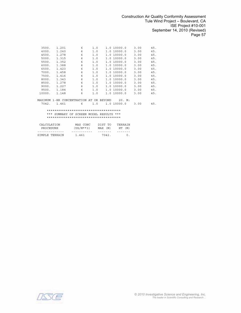
Construction Air Quality Conformity AssessmentTule Wind Project – Boulevard, CA
ISE Project #10-001September 14, 2010 (Revised)
Page 57
© 2010 Investigative Science and Engineering, Inc. The leader in Scientific Consulting and Research…
3500. 1.201 6 1.0 1.0 10000.0 3.00 45. 4000. 1.240 6 1.0 1.0 10000.0 3.00 45. 4500. 1.278 6 1.0 1.0 10000.0 3.00 45. 5000. 1.315 6 1.0 1.0 10000.0 3.00 45. 5500. 1.352 6 1.0 1.0 10000.0 3.00 45. 6000. 1.388 6 1.0 1.0 10000.0 3.00 45. 6500. 1.423 6 1.0 1.0 10000.0 3.00 45. 7000. 1.458 6 1.0 1.0 10000.0 3.00 45. 7500. 1.416 6 1.0 1.0 10000.0 3.00 45. 8000. 1.343 6 1.0 1.0 10000.0 3.00 45. 8500. 1.278 6 1.0 1.0 10000.0 3.00 45. 9000. 1.227 6 1.0 1.0 10000.0 3.00 45. 9500. 1.184 6 1.0 1.0 10000.0 3.00 45. 10000. 1.148 6 1.0 1.0 10000.0 3.00 45.
MAXIMUM 1-HR CONCENTRATION AT OR BEYOND 20. M: 7042. 1.461 6 1.0 1.0 10000.0 3.00 45.
*************************************** *** SUMMARY OF SCREEN MODEL RESULTS *** ***************************************
CALCULATION MAX CONC DIST TO TERRAIN PROCEDURE (UG/M**3) MAX (M) HT (M)-------------- ----------- ------- -------
SIMPLE TERRAIN 1.461 7042. 0.
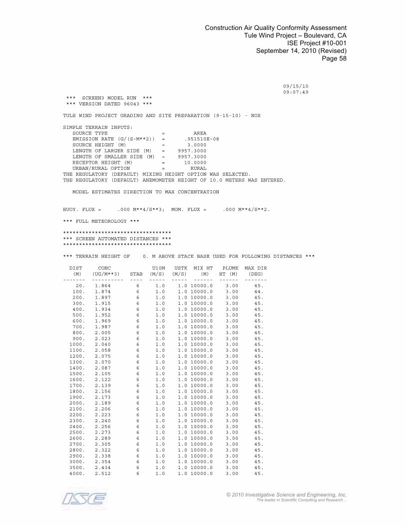
Construction Air Quality Conformity AssessmentTule Wind Project – Boulevard, CA
ISE Project #10-001September 14, 2010 (Revised)
Page 58
© 2010 Investigative Science and Engineering, Inc. The leader in Scientific Consulting and Research…
09/15/10 09:07:49 *** SCREEN3 MODEL RUN *** *** VERSION DATED 96043 ***
TULE WIND PROJECT GRADING AND SITE PREPARATION (9-15-10) - NOX
SIMPLE TERRAIN INPUTS: SOURCE TYPE = AREA EMISSION RATE (G/(S-M**2)) = .951510E-08 SOURCE HEIGHT (M) = 3.0000 LENGTH OF LARGER SIDE (M) = 9957.3000 LENGTH OF SMALLER SIDE (M) = 9957.3000 RECEPTOR HEIGHT (M) = 10.0000 URBAN/RURAL OPTION = RURAL THE REGULATORY (DEFAULT) MIXING HEIGHT OPTION WAS SELECTED. THE REGULATORY (DEFAULT) ANEMOMETER HEIGHT OF 10.0 METERS WAS ENTERED.
MODEL ESTIMATES DIRECTION TO MAX CONCENTRATION
BUOY. FLUX = .000 M**4/S**3; MOM. FLUX = .000 M**4/S**2.
*** FULL METEOROLOGY ***
********************************** *** SCREEN AUTOMATED DISTANCES *** **********************************
*** TERRAIN HEIGHT OF 0. M ABOVE STACK BASE USED FOR FOLLOWING DISTANCES ***
DIST CONC U10M USTK MIX HT PLUME MAX DIR (M) (UG/M**3) STAB (M/S) (M/S) (M) HT (M) (DEG)------- ---------- ---- ----- ----- ------ ------ -------
20. 1.864 6 1.0 1.0 10000.0 3.00 45. 100. 1.874 6 1.0 1.0 10000.0 3.00 44. 200. 1.897 6 1.0 1.0 10000.0 3.00 45. 300. 1.915 6 1.0 1.0 10000.0 3.00 45.
400. 1.934 6 1.0 1.0 10000.0 3.00 45. 500. 1.952 6 1.0 1.0 10000.0 3.00 45. 600. 1.969 6 1.0 1.0 10000.0 3.00 45. 700. 1.987 6 1.0 1.0 10000.0 3.00 45. 800. 2.005 6 1.0 1.0 10000.0 3.00 45. 900. 2.023 6 1.0 1.0 10000.0 3.00 45. 1000. 2.040 6 1.0 1.0 10000.0 3.00 45. 1100. 2.058 6 1.0 1.0 10000.0 3.00 45. 1200. 2.075 6 1.0 1.0 10000.0 3.00 45. 1300. 2.070 6 1.0 1.0 10000.0 3.00 45. 1400. 2.087 6 1.0 1.0 10000.0 3.00 45. 1500. 2.105 6 1.0 1.0 10000.0 3.00 45. 1600. 2.122 6 1.0 1.0 10000.0 3.00 45. 1700. 2.139 6 1.0 1.0 10000.0 3.00 45. 1800. 2.156 6 1.0 1.0 10000.0 3.00 45. 1900. 2.173 6 1.0 1.0 10000.0 3.00 45. 2000. 2.189 6 1.0 1.0 10000.0 3.00 45. 2100. 2.206 6 1.0 1.0 10000.0 3.00 45. 2200. 2.223 6 1.0 1.0 10000.0 3.00 45. 2300. 2.240 6 1.0 1.0 10000.0 3.00 45. 2400. 2.256 6 1.0 1.0 10000.0 3.00 45. 2500. 2.273 6 1.0 1.0 10000.0 3.00 45. 2600. 2.289 6 1.0 1.0 10000.0 3.00 45. 2700. 2.305 6 1.0 1.0 10000.0 3.00 45. 2800. 2.322 6 1.0 1.0 10000.0 3.00 45. 2900. 2.338 6 1.0 1.0 10000.0 3.00 45. 3000. 2.354 6 1.0 1.0 10000.0 3.00 45. 3500. 2.434 6 1.0 1.0 10000.0 3.00 45. 4000. 2.512 6 1.0 1.0 10000.0 3.00 45.
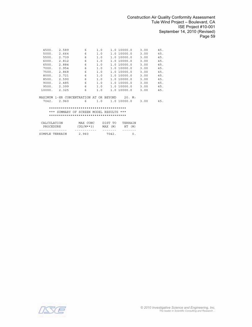
Construction Air Quality Conformity AssessmentTule Wind Project – Boulevard, CA
ISE Project #10-001September 14, 2010 (Revised)
Page 59
© 2010 Investigative Science and Engineering, Inc. The leader in Scientific Consulting and Research…
4500. 2.589 6 1.0 1.0 10000.0 3.00 45. 5000. 2.664 6 1.0 1.0 10000.0 3.00 45. 5500. 2.739 6 1.0 1.0 10000.0 3.00 45. 6000. 2.812 6 1.0 1.0 10000.0 3.00 45. 6500. 2.884 6 1.0 1.0 10000.0 3.00 45. 7000. 2.954 6 1.0 1.0 10000.0 3.00 45. 7500. 2.868 6 1.0 1.0 10000.0 3.00 45. 8000. 2.721 6 1.0 1.0 10000.0 3.00 45. 8500. 2.590 6 1.0 1.0 10000.0 3.00 45. 9000. 2.485 6 1.0 1.0 10000.0 3.00 45. 9500. 2.399 6 1.0 1.0 10000.0 3.00 45. 10000. 2.325 6 1.0 1.0 10000.0 3.00 45.
MAXIMUM 1-HR CONCENTRATION AT OR BEYOND 20. M: 7042. 2.960 6 1.0 1.0 10000.0 3.00 45.
*************************************** *** SUMMARY OF SCREEN MODEL RESULTS *** ***************************************
CALCULATION MAX CONC DIST TO TERRAIN PROCEDURE (UG/M**3) MAX (M) HT (M)-------------- ----------- ------- -------
SIMPLE TERRAIN 2.960 7042. 0.

Construction Air Quality Conformity AssessmentTule Wind Project – Boulevard, CA
ISE Project #10-001September 14, 2010 (Revised)
Page 60
© 2010 Investigative Science and Engineering, Inc. The leader in Scientific Consulting and Research…
09/15/10 09:07:49 *** SCREEN3 MODEL RUN *** *** VERSION DATED 96043 ***
TULE WIND PROJECT GRADING AND SITE PREPARATION (9-15-10) - SOX
SIMPLE TERRAIN INPUTS: SOURCE TYPE = AREA EMISSION RATE (G/(S-M**2)) = .878970E-09 SOURCE HEIGHT (M) = 3.0000 LENGTH OF LARGER SIDE (M) = 9957.3000 LENGTH OF SMALLER SIDE (M) = 9957.3000 RECEPTOR HEIGHT (M) = 10.0000 URBAN/RURAL OPTION = RURAL THE REGULATORY (DEFAULT) MIXING HEIGHT OPTION WAS SELECTED. THE REGULATORY (DEFAULT) ANEMOMETER HEIGHT OF 10.0 METERS WAS ENTERED.
MODEL ESTIMATES DIRECTION TO MAX CONCENTRATION
BUOY. FLUX = .000 M**4/S**3; MOM. FLUX = .000 M**4/S**2.
*** FULL METEOROLOGY ***
********************************** *** SCREEN AUTOMATED DISTANCES *** **********************************
*** TERRAIN HEIGHT OF 0. M ABOVE STACK BASE USED FOR FOLLOWING DISTANCES ***
DIST CONC U10M USTK MIX HT PLUME MAX DIR (M) (UG/M**3) STAB (M/S) (M/S) (M) HT (M) (DEG)------- ---------- ---- ----- ----- ------ ------ -------
20. .1722 6 1.0 1.0 10000.0 3.00 45. 100. .1731 6 1.0 1.0 10000.0 3.00 44. 200. .1753 6 1.0 1.0 10000.0 3.00 45. 300. .1769 6 1.0 1.0 10000.0 3.00 45. 400. .1786 6 1.0 1.0 10000.0 3.00 45. 500. .1803 6 1.0 1.0 10000.0 3.00 45. 600. .1819 6 1.0 1.0 10000.0 3.00 45. 700. .1836 6 1.0 1.0 10000.0 3.00 45. 800. .1852 6 1.0 1.0 10000.0 3.00 45. 900. .1869 6 1.0 1.0 10000.0 3.00 45. 1000. .1885 6 1.0 1.0 10000.0 3.00 45. 1100. .1901 6 1.0 1.0 10000.0 3.00 45. 1200. .1917 6 1.0 1.0 10000.0 3.00 45. 1300. .1912 6 1.0 1.0 10000.0 3.00 45. 1400. .1928 6 1.0 1.0 10000.0 3.00 45. 1500. .1944 6 1.0 1.0 10000.0 3.00 45. 1600. .1960 6 1.0 1.0 10000.0 3.00 45. 1700. .1976 6 1.0 1.0 10000.0 3.00 45. 1800. .1991 6 1.0 1.0 10000.0 3.00 45. 1900. .2007 6 1.0 1.0 10000.0 3.00 45. 2000. .2023 6 1.0 1.0 10000.0 3.00 45. 2100. .2038 6 1.0 1.0 10000.0 3.00 45. 2200. .2053 6 1.0 1.0 10000.0 3.00 45. 2300. .2069 6 1.0 1.0 10000.0 3.00 45. 2400. .2084 6 1.0 1.0 10000.0 3.00 45. 2500. .2099 6 1.0 1.0 10000.0 3.00 45. 2600. .2114 6 1.0 1.0 10000.0 3.00 45. 2700. .2130 6 1.0 1.0 10000.0 3.00 45. 2800. .2145 6 1.0 1.0 10000.0 3.00 45. 2900. .2160 6 1.0 1.0 10000.0 3.00 45. 3000. .2174 6 1.0 1.0 10000.0 3.00 45. 3500. .2248 6 1.0 1.0 10000.0 3.00 45. 4000. .2321 6 1.0 1.0 10000.0 3.00 45.

Construction Air Quality Conformity AssessmentTule Wind Project – Boulevard, CA
ISE Project #10-001September 14, 2010 (Revised)
Page 61
© 2010 Investigative Science and Engineering, Inc. The leader in Scientific Consulting and Research…
4500. .2392 6 1.0 1.0 10000.0 3.00 45. 5000. .2461 6 1.0 1.0 10000.0 3.00 45. 5500. .2530 6 1.0 1.0 10000.0 3.00 45. 6000. .2598 6 1.0 1.0 10000.0 3.00 45. 6500. .2664 6 1.0 1.0 10000.0 3.00 45. 7000. .2729 6 1.0 1.0 10000.0 3.00 45. 7500. .2650 6 1.0 1.0 10000.0 3.00 45. 8000. .2513 6 1.0 1.0 10000.0 3.00 45. 8500. .2393 6 1.0 1.0 10000.0 3.00 45. 9000. .2296 6 1.0 1.0 10000.0 3.00 45. 9500. .2216 6 1.0 1.0 10000.0 3.00 45. 10000. .2148 6 1.0 1.0 10000.0 3.00 45.
MAXIMUM 1-HR CONCENTRATION AT OR BEYOND 20. M: 7042. .2734 6 1.0 1.0 10000.0 3.00 45.
*************************************** *** SUMMARY OF SCREEN MODEL RESULTS *** ***************************************
CALCULATION MAX CONC DIST TO TERRAIN PROCEDURE (UG/M**3) MAX (M) HT (M)-------------- ----------- ------- -------
SIMPLE TERRAIN .2734 7042. 0.

Construction Air Quality Conformity AssessmentTule Wind Project – Boulevard, CA
ISE Project #10-001September 14, 2010 (Revised)
Page 62
© 2010 Investigative Science and Engineering, Inc. The leader in Scientific Consulting and Research…
09/15/10 09:07:49 *** SCREEN3 MODEL RUN *** *** VERSION DATED 96043 ***
TULE WIND PROJECT GRADING AND SITE PREPARATION (9-15-10) - PM10
SIMPLE TERRAIN INPUTS: SOURCE TYPE = AREA EMISSION RATE (G/(S-M**2)) = .587750E-09 SOURCE HEIGHT (M) = 3.0000 LENGTH OF LARGER SIDE (M) = 9957.3000 LENGTH OF SMALLER SIDE (M) = 9957.3000 RECEPTOR HEIGHT (M) = 10.0000 URBAN/RURAL OPTION = RURAL THE REGULATORY (DEFAULT) MIXING HEIGHT OPTION WAS SELECTED. THE REGULATORY (DEFAULT) ANEMOMETER HEIGHT OF 10.0 METERS WAS ENTERED.
MODEL ESTIMATES DIRECTION TO MAX CONCENTRATION
BUOY. FLUX = .000 M**4/S**3; MOM. FLUX = .000 M**4/S**2.
*** FULL METEOROLOGY ***
********************************** *** SCREEN AUTOMATED DISTANCES *** **********************************
*** TERRAIN HEIGHT OF 0. M ABOVE STACK BASE USED FOR FOLLOWING DISTANCES ***
DIST CONC U10M USTK MIX HT PLUME MAX DIR (M) (UG/M**3) STAB (M/S) (M/S) (M) HT (M) (DEG)------- ---------- ---- ----- ----- ------ ------ -------
20. .1151 6 1.0 1.0 10000.0 3.00 45. 100. .1158 6 1.0 1.0 10000.0 3.00 44. 200. .1172 6 1.0 1.0 10000.0 3.00 45. 300. .1183 6 1.0 1.0 10000.0 3.00 45. 400. .1194 6 1.0 1.0 10000.0 3.00 45. 500. .1205 6 1.0 1.0 10000.0 3.00 45. 600. .1217 6 1.0 1.0 10000.0 3.00 45. 700. .1228 6 1.0 1.0 10000.0 3.00 45. 800. .1239 6 1.0 1.0 10000.0 3.00 45. 900. .1249 6 1.0 1.0 10000.0 3.00 45. 1000. .1260 6 1.0 1.0 10000.0 3.00 45. 1100. .1271 6 1.0 1.0 10000.0 3.00 45. 1200. .1282 6 1.0 1.0 10000.0 3.00 45. 1300. .1279 6 1.0 1.0 10000.0 3.00 45. 1400. .1289 6 1.0 1.0 10000.0 3.00 45. 1500. .1300 6 1.0 1.0 10000.0 3.00 45. 1600. .1311 6 1.0 1.0 10000.0 3.00 45. 1700. .1321 6 1.0 1.0 10000.0 3.00 45. 1800. .1332 6 1.0 1.0 10000.0 3.00 45. 1900. .1342 6 1.0 1.0 10000.0 3.00 45. 2000. .1352 6 1.0 1.0 10000.0 3.00 45. 2100. .1363 6 1.0 1.0 10000.0 3.00 45. 2200. .1373 6 1.0 1.0 10000.0 3.00 45. 2300. .1383 6 1.0 1.0 10000.0 3.00 45. 2400. .1394 6 1.0 1.0 10000.0 3.00 45. 2500. .1404 6 1.0 1.0 10000.0 3.00 45. 2600. .1414 6 1.0 1.0 10000.0 3.00 45. 2700. .1424 6 1.0 1.0 10000.0 3.00 45. 2800. .1434 6 1.0 1.0 10000.0 3.00 45. 2900. .1444 6 1.0 1.0 10000.0 3.00 45. 3000. .1454 6 1.0 1.0 10000.0 3.00 45. 3500. .1503 6 1.0 1.0 10000.0 3.00 45. 4000. .1552 6 1.0 1.0 10000.0 3.00 45.

Construction Air Quality Conformity AssessmentTule Wind Project – Boulevard, CA
ISE Project #10-001September 14, 2010 (Revised)
Page 63
© 2010 Investigative Science and Engineering, Inc. The leader in Scientific Consulting and Research…
4500. .1599 6 1.0 1.0 10000.0 3.00 45. 5000. .1646 6 1.0 1.0 10000.0 3.00 45. 5500. .1692 6 1.0 1.0 10000.0 3.00 45. 6000. .1737 6 1.0 1.0 10000.0 3.00 45. 6500. .1781 6 1.0 1.0 10000.0 3.00 45. 7000. .1825 6 1.0 1.0 10000.0 3.00 45. 7500. .1772 6 1.0 1.0 10000.0 3.00 45. 8000. .1681 6 1.0 1.0 10000.0 3.00 45. 8500. .1600 6 1.0 1.0 10000.0 3.00 45. 9000. .1535 6 1.0 1.0 10000.0 3.00 45. 9500. .1482 6 1.0 1.0 10000.0 3.00 45. 10000. .1436 6 1.0 1.0 10000.0 3.00 45.
MAXIMUM 1-HR CONCENTRATION AT OR BEYOND 20. M: 7042. .1828 6 1.0 1.0 10000.0 3.00 45.
*************************************** *** SUMMARY OF SCREEN MODEL RESULTS *** ***************************************
CALCULATION MAX CONC DIST TO TERRAIN PROCEDURE (UG/M**3) MAX (M) HT (M)-------------- ----------- ------- -------
SIMPLE TERRAIN .1828 7042. 0.

Construction Air Quality Conformity AssessmentTule Wind Project – Boulevard, CA
ISE Project #10-001September 14, 2010 (Revised)
Page 64
© 2010 Investigative Science and Engineering, Inc. The leader in Scientific Consulting and Research…
CALINE4 SOLUTION SPACE RESULTS – SCENARIO CO
Rank 1 Eqn 151232682 lnz=a+blnx+c(lny)2
r2 Coef Det DF Adj r2 Fit Std Err F-value0.9997614637 0.9997516609 0.102880788 155075.68815
Parm Value Std Error t-value 95.00% Confidence Limits P>|t| a -5.38627658 0.022750405 -236.75519 -5.43160775 -5.34094541 0.00000 b 0.999812043 0.003657036 273.3940571 0.992525238 1.007098847 0.00000 c 0.048869087 0.000171868 284.3402911 0.048526632 0.049211542 0.00000
CONC
VPH
EMFAC

Construction Air Quality Conformity AssessmentTule Wind Project – Boulevard, CA
ISE Project #10-001September 14, 2010 (Revised)
Page 65
© 2010 Investigative Science and Engineering, Inc. The leader in Scientific Consulting and Research…
CALINE4 SOLUTION SPACE RESULTS – SCENARIO NOX
Rank 1 Eqn 151232653 lnz=a+bx0.5+c(lny)2
r2 Coef Det DF Adj r2 Fit Std Err F-value0.9311638335 0.9283349499 0.0194986151 500.50814223
Parm Value Std Error t-value 95.00% Confidence Limits P>|t| a -5.48793064 0.131941715 -41.593598 -5.75083025 -5.22503104 0.00000 b 0.756396215 0.037072879 20.40295328 0.682526891 0.830265538 0.00000 c 0.023350423 0.001103789 21.15477893 0.021151074 0.025549771 0.00000
CONC
VPH
EMFAC

Construction Air Quality Conformity AssessmentTule Wind Project – Boulevard, CA
ISE Project #10-001September 14, 2010 (Revised)
Page 66
© 2010 Investigative Science and Engineering, Inc. The leader in Scientific Consulting and Research…
CALINE4 SOLUTION SPACE RESULTS – SCENARIO PM10
Rank 1 Eqn 151232682 lnz=a+blnx+c(lny)2
r2 Coef Det DF Adj r2 Fit Std Err F-value0.9998185376 0.9998110803 2.1625247335 203862.00724
Parm Value Std Error t-value 95.00% Confidence Limits P>|t| a 1.706831053 0.01706339 100.0288368 1.672831506 1.7408306 0.00000 b 0.999960683 0.003187502 313.7129842 0.993609447 1.006311919 0.00000 c 0.048878379 0.000149717 326.4708691 0.048580061 0.049176698 0.00000
CONC
VPH
EMFAC

Construction Air Quality Conformity AssessmentTule Wind Project – Boulevard, CA
ISE Project #10-001September 14, 2010 (Revised)
Page 67
© 2010 Investigative Science and Engineering, Inc. The leader in Scientific Consulting and Research…
INDEX OF IMPORTANT TERMS
atomic mass, 41
CAAQS, 14, 19, 46, 47, 49California Air Resources Board, 14, 22California Ambient Air Quality Standards, 14California Environmental Quality Act, 14, 17CALINE4, 30, 64, 65, 66cancer, 20, 27, 28, 46CARB, 14, 15, 21, 22, 25, 28, 29, 33, 34, 35,
36, 37, 38, 39, 40, 52Carbon Monoxide, 12, 18, 20, 29, 30CEIDARS, 26, 29, 47CEQA, 14, 17, 18, 19, 21, 26, 44, 50Clean Air Act, 14, 18CO, 12, 18, 19, 22, 25, 26, 30, 33, 42, 47,
49, 50, 51, 52, 56, 64Consistency Criterion, 53control efficiency, 45
de minimis, 19
EMFAC 2007, 29, 30, 50, 54Environmental Protection Agency, 12EPA, 12, 14, 15, 18, 19, 24, 25, 27, 41
hydrocarbons, 13Hydrogen Sulfide, 12, 13, 20
ISE, 1, 2, 3, 11, 23, 25, 32, 48, 53
mass spectrometer, 24Motor Vehicle Emission Inventory, 28MVEI, 28, 29
NAAQS, 14, 48, 49National Ambient Air Quality Standards, 14National Institute of Standards and
Technology, 22, 25Nitrogen Dioxide, 12, 20NO2, 12NOx, 22, 25, 26
O3, 12, 13, 22, 33odor, 13, 49
Ozone, 12, 13, 33
PAH, 20particulate matter, 12, 42PM10, 12, 13, 18, 22, 25, 26, 27, 29, 30, 33,
35, 42, 43, 44, 45, 46, 47, 48, 49, 50, 51, 52, 56, 66
PM2.5, 26, 33polynuclear aromatic hydrocarbons, 20
Radiation inversion, 31Reactive Organic Gasses, 12, 13Reference Exposure Levels, 20REL, 21risk, 13, 20, 21, 27, 28, 46, 47ROG, 12, 13, 18, 25, 42, 50, 52
San Diego Air Pollution Control District, 17Santa Ana Conditions, 31SCAQMD, 18, 21, 26, 27, 29, 44, 45SCREEN3, 27, 46, 47, 56SDAPCD, 17, 18, 19, 22, 45, 50, 52SO2, 12, 13, 14SOx, 26Spectral deconvolution, 41Standard Temperature and Pressure, 24STP, 24, 47Subsidence inversions, 31Sulfur Dioxide, 12, 20
T-BACT, 21, 46Tedlar, 24Tier 0, 25Tier 2, 25, 26Tier 3, 26Toxic Best Available Control Technologies,
21
UGA, 24Universal Gas Analyzer, 24
VOC, 12, 13, 18, 52Volatile Organic Compounds, 12, 13


ACOUSTICS – VIBRATION – AIR & WATER QUALITY – FORENSIC ENGINEERING EXPERT WITNESS – ENVIRONMENTAL ASSESSMENTS AND COMPLIANCE
GREENHOUSE GAS / GLOBAL WARMING RISK ASSESSMENT
TULE WIND PROJECTBOULEVARD, CA
Submitted to:
Mr. Patrick O'NeillHDR
8690 Balboa Avenue, Suite 200San Diego, CA 92123
Investigative Science and Engineering, Inc. Scientific, Environmental, and Forensic Consultants
P.O. Box 488 / 1134 D StreetRamona, CA 92065
(760) 787-0016www.ise.us
ISE Project #10-001
September 14, 2010 (Revised)


© 2010 Investigative Science and Engineering, Inc. The leader in Scientific Consulting and Research…
REPORT CONTENTS
INTRODUCTION AND DEFINITIONS 1
Existing Site Characterization 1
Project Description 1
Historical Context of Global Warming Theories 12
Greenhouse Gases and Global Warming Potential 14
THRESHOLDS OF SIGNIFICANCE 18
California Environmental Quality Act (CEQA) Thresholds 18
The California Global Warming Solutions Act (AB 32) 18
CAPCOA Recommended CO2e Screening Levels 19
ANALYSIS METHODOLOGY 20
Greenhouse Gas Compilation Approach 20
Projected Greenhouse Gas Emissions Budget and Warming Effects Analysis 21
FINDINGS 21
Greenhouse Gas Emission Tabulation 21
Projected Project Greenhouse Gas Emissions Budget 23
Projected Warming Effects Due to Project Equivalent CO2e 24
CONCLUSIONS / RECOMMENDATIONS 26
Project-Related Greenhouse Gas Budget / Global Warming Potential 26
Compliance with AB 32 CO2 Reduction Strategies 26
CERTIFICATION OF ACCURACY AND QUALIFICATIONS 27
APPENDICES / SUPPLEMENTAL INFORMATION 28
EMFAC 2007 EMISSION FACTOR TABULATIONS – SCENARIO YEAR 2012 28
INDEX OF IMPORTANT TERMS 29

© 2010 Investigative Science and Engineering, Inc. The leader in Scientific Consulting and Research…
LIST OF TABLES
TABLE 1: Known Greenhouse Gases and Global Warming Potential 16TABLE 2: Construction Vehicle GHG Emission Levels – Tule Wind Project (Tier 0) 22TABLE 3: Construction Worker Vehicle GHG Levels – Tule Wind Project 23TABLE 4: GHG Emission Budget for Tule Wind Project 23
LIST OF FIGURES / MAPS / ADDENDA
FIGURE 1a: Project Area Vicinity Map 2
FIGURE 1b: Project Jurisdictional Land Use Map 3
FIGURE 2a: Proposed Tule Wind Project Overview Map 4
FIGURE 2b: Proposed Tule Wind Project Turbine Configuration – Sheet 1 5
FIGURE 2c: Proposed Tule Wind Project Turbine Configuration – Sheet 2 6
FIGURE 2d: Proposed Tule Wind Project Turbine Configuration – Sheet 3 7
FIGURE 2e: Proposed Tule Wind Project Turbine Configuration – Sheet 4 8
FIGURE 3: Proposed Tule Wind Project Access Road Configuration 9
FIGURE 4: Isometric Aerial Photograph w/ Proposed Project Uses 11
FIGURE 5: Measured/Predicted Global Temperature Variations 13

© 2010 Investigative Science and Engineering, Inc. The leader in Scientific Consulting and Research…
INTRODUCTION AND DEFINITIONS
Existing Site Characterization
The project site has an effective working footprint of 38.3 square-miles (24,500acres)1 located in the eastern portion of San Diego County in the community of Boulevard, CA as shown in Figure 1a on the following page. Regional access to the site is obtained from the Ribbonwood Road exit, off Interstate 8 (I-8) and McCain Valley Road.
The development site consists of steep and rugged terrain areas located primarily on federal lands managed by the Bureau of Land Management (BLM), or other public lands, such as those maintained by the California State Lands Commission, and the Cuyapaipe Band of Mission Indians (denoted as the red shaded areas, as shown in Figure 1b on Page 3 of this report). A small portion of the project site resides on privately owned lands under the jurisdiction of the County of San Diego, with the majority of the project area being outside the land use jurisdiction of the County of San Diego. Elevations across the site are markedly varied and range from approximately 3,500 to 5,600 feet above mean sea level (MSL).
Project Description
The Tule Wind Project proposes the construction of a 200-megawatt (MW) wind turbine power generating facility within the McCain Valley area of eastern San Diego County. Pacific Wind Development LLC is proposing to construct and operate the Tule Wind Project located near Boulevard, California. The proposed wind generation project will consist of the following components:
• Up to 134 wind turbines, ranging in size between 328 and 492 feet in height, to produce 200 MW of electricity, as denoted in Figures 2a through -e starting on Page 4 of this report;
• Construct a five-acre collector substation and five-acre operation and maintenance (O&M) facility as denoted as brown polygons in Figures 2a through -e;
• Construct a 34.5 kV electrical collector grid (denoted as –E– in Figures 2a through -e) connecting the turbines to the collector substation, and construct a 138-kilovolt (kV) overhead and underground transmission line (denoted as –T– in Figures 2a through -e) running south from the proposed substation to the San Diego Gas & Electric (SDG&E) Boulevard Substation;
• Construct access roads between turbines and perform improvements to existing roadways, as denoted in red in Figure 3 on Page 9 of this report;
• Construct a temporary five-acre batch plant for construction activities, as well as a temporary 10-acre parking area, and nineteen two-acre lay down areas; and,
• Construct two permanent meteorological towers and one SODAR Unit. 1 Determined to consist of the worst-case polygon enclosing the turbine locations and access roads shown in Figure 3 of this report.

Greenhouse Gas / Global Warming Risk AssessmentTule Wind Project – Boulevard, CA
ISE Project #10-001September 14, 2010 (Revised)
Page 2
© 2010 Investigative Science and Engineering, Inc. The leader in Scientific Consulting and Research…
FIGURE 1a: Project Area Vicinity Map (ISE 9/10)

Greenhouse Gas / Global Warming Risk AssessmentTule Wind Project – Boulevard, CA
ISE Project #10-001September 14, 2010 (Revised)
Page 3
© 2010 Investigative Science and Engineering, Inc. The leader in Scientific Consulting and Research…
FIGURE 1b: Project Jurisdictional Land Use Map (ISE 9/10)

Greenhouse Gas / Global Warming Risk AssessmentTule Wind Project – Boulevard, CA
ISE Project #10-001September 14, 2010 (Revised)
Page 4
© 2010 Investigative Science and Engineering, Inc. The leader in Scientific Consulting and Research…
FIGURE 2a: Proposed Tule Wind Project Overview Map (ISE 9/10)

Greenhouse Gas / Global Warming Risk AssessmentTule Wind Project – Boulevard, CA
ISE Project #10-001September 14, 2010 (Revised)
Page 5
© 2010 Investigative Science and Engineering, Inc. The leader in Scientific Consulting and Research…
FIGURE 2b: Proposed Tule Wind Project Turbine Configuration – Sheet 1 (ISE 9/10)

Greenhouse Gas / Global Warming Risk AssessmentTule Wind Project – Boulevard, CA
ISE Project #10-001September 14, 2010 (Revised)
Page 6
© 2010 Investigative Science and Engineering, Inc. The leader in Scientific Consulting and Research…
FIGURE 2c: Proposed Tule Wind Project Turbine Configuration – Sheet 2 (ISE 9/10)

Greenhouse Gas / Global Warming Risk AssessmentTule Wind Project – Boulevard, CA
ISE Project #10-001September 14, 2010 (Revised)
Page 7
© 2010 Investigative Science and Engineering, Inc. The leader in Scientific Consulting and Research…
FIGURE 2d: Proposed Tule Wind Project Turbine Configuration – Sheet 3 (ISE 9/10)
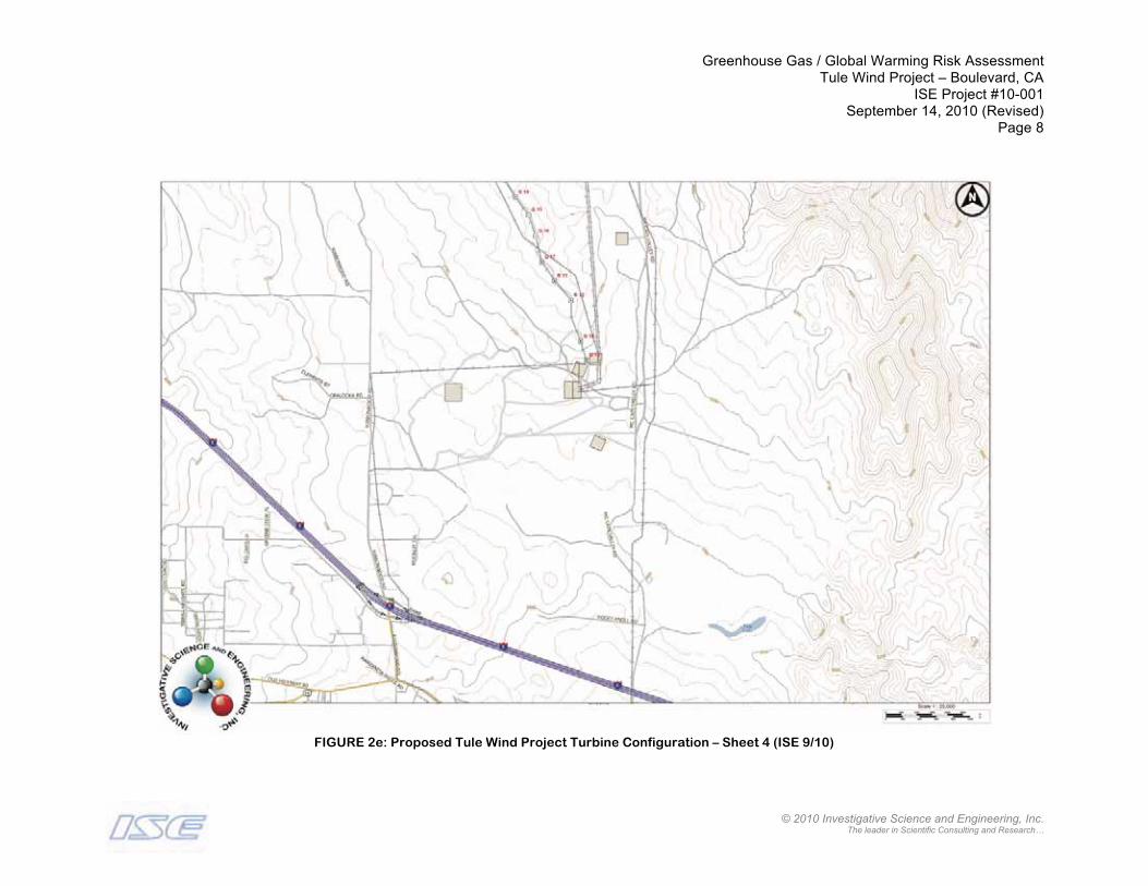
Greenhouse Gas / Global Warming Risk AssessmentTule Wind Project – Boulevard, CA
ISE Project #10-001September 14, 2010 (Revised)
Page 8
© 2010 Investigative Science and Engineering, Inc. The leader in Scientific Consulting and Research…
FIGURE 2e: Proposed Tule Wind Project Turbine Configuration – Sheet 4 (ISE 9/10)

Greenhouse Gas / Global Warming Risk AssessmentTule Wind Project – Boulevard, CA
ISE Project #10-001September 14, 2010 (Revised)
Page 9
© 2010 Investigative Science and Engineering, Inc. The leader in Scientific Consulting and Research…
FIGURE 3: Proposed Tule Wind Project Access Road Configuration (ISE 9/10)

Greenhouse Gas / Global Warming Risk AssessmentTule Wind Project – Boulevard, CA
ISE Project #10-001September 14, 2010 (Revised)
Page 10
© 2010 Investigative Science and Engineering, Inc. The leader in Scientific Consulting and Research…
Project construction activities will avoid excessive grading on roads, road embankments, ditches, and drainages to the extent possible to maintain a minimal footprint. A temporary construction work area will be cleared for each wind turbine tower. Work areas may vary in size, and may be constructed differently in keeping with each site’s topography (although for the purposes of analysis within this report, an average estimate of construction effort will be examined). The proposed construction influence area (and subsequent study area within this report) is shown in Figure 4 on the following page.
Each turbine work area will require up to a 200-foot radius to be cleared and leveled. The cleared area is necessary for foundation excavation and construction, assembling turbine sections, and also to stage the construction crane, which will hoist turbine sections into place. The turbine construction area will not be paved. Permanent wind tower foundations will be approximately 60 feet in diameter, and seven to ten feet in depth. After turbine erection has been completed, a 9 to 10-foot wide area around the base of the tower will be surfaced with gravel. The gravel will provide a stable surface area for maintenance vehicles, and will minimize surface erosion and runoff.
Underground electrical and communications cables will be placed in a 3 to 5-foot wide, and 3 to 5-foot deep trench, generally along the length of the proposed turbine access roads. Electrical cables will be installed first and the trench will be partially backfilled before placing communications cables. The topsoil in the trench will be stripped and set aside before the trench is backfilled, with topsoil replaced on the uppermost layer. Concrete or fiberglass vaults and splice boxes will be placed at necessary locations. Boxes will have locked lids to prevent public access. The vaults will be about 5 x 5 x 8 feet, and will be placed approximately 2,500 feet apart.
Aboveground collector lines will use steel poles that are 60 to 80 feet in height; taller heights may be needed to cross washes or drainages. Aboveground lines are normally used to span canyons or streams to eliminate the habitat disturbance that trenching causes in these areas. The interconnection transmission line, operating at a voltage of 138 kV, and leading from the Project substation to the Boulevard substation will be above ground for all or a portion of its length. The exact location for transmission poles will be determined closer to final engineering and design.
Finally, roads will be designed in accordance with County Standards. Transportation routing will be conducted to minimize impacts to normal traffic flow during the transport of turbine components, main assembly cranes, and other large pieces of equipment. After construction is complete, the applicant will work to restore vegetation to pre-construction standards for all disturbed areas.

Greenhouse Gas / Global Warming Risk AssessmentTule Wind Project – Boulevard, CA
ISE Project #10-001September 14, 2010 (Revised)
Page 11
© 2010 Investigative Science and Engineering, Inc. The leader in Scientific Consulting and Research…
FIGURE 4: Isometric Aerial Photograph w/ Proposed Project Uses (ISE 9/10)
Greenhouse Gas / Global Warming Risk AssessmentTule Wind Project – Boulevard, CA
ISE Project #10-001September 14, 2010 (Revised)
Page 12
© 2010 Investigative Science and Engineering, Inc. The leader in Scientific Consulting and Research…
Upon completion of construction, the project would be supported by up to 10
permanent full-time or part-time employees on the Operations and Maintenance (O&M) staff. Typically, these staff will be present on site during normal business hours.Maintenance activities will be limited to areas accessible by the permanent access roadsprovided during the construction phase. Each turbine would be serviced approximately twice a year. Turbine servicing activities might include temporarily deploying a crane, removing the turbine rotor, replacing generators, bearings, and deploying personnel to climb the towers to service parts within the turbine.
Computer systems inside each turbine would perform self-diagnostic tests and allow a remote operator to set new operating parameters, perform system checks, and ensure turbines are operating at peak performance. Turbines would automatically shut down if sustained winds reach 50 miles per hour (mph) or gusts reach about 56 mph.There would be no operational air quality issues associated with the proposed Tule Wind Project. Historical Context of Global Warming Theories
Much recent conjecture has been postulated as to the effect of the so-called, ‘Global Warming Phenomenon’ or ‘Greenhouse Gas Effect’ and its correlation to anthropogenic ‘Greenhouse Gas (GHG) Emissions’.2 The debate began based upon initial observations that global surface temperatures have been perceived to be steadily increasing over the past century (i.e., the period for which competent and reliable measurements have been taken), with an increase of roughly 0.6 degrees Centigrade,as can be seen in the first pane of Figure 5 on the following page.3,4,5
2 In fact, the notion that manmade (anthropogenic) global warming was a possibility has existed in written documentation since the early 1880’s and been the subject of much chicanery within the realms of scientific fact as well as that of science fiction. Arguments have ranged from anecdotal cause-and-effect relationships to outright claims of disaster such as sea ice melting at great rates causing precipitous rises in global ocean levels (a clear violation of Archimedes' principle discovered over 2,200 years ago). It is safe to say that the dynamics of anthropogenic global warming and/or cooling is a less than well-defined field of science.3 The majority of this increase in temperature, which is formally expressed by the United Nations Intergovernmental Panel on Climate Change (IPCC) as 0.6 ± 0.2 degrees Centigrade, occurred before 1940 AD, the generally accepted date when anthropogenic atmospheric CO2 levels started any noticeable increase. The data presented in the first pane of Figure 5 provides information from surface temperature stations (red bars), as well as the annual average (the black trend line). The gray bars indicate the 95-percent confidence limits on the data. The black global temperature line (which is the basis of the whole global temperature increase argument) is only as good as the bounds of the gray tick-marks (which can have errors as large as, or larger than, the data point being represented).4 Source: IPCC, 2001, Climate Change 2001: The Scientific Basis. Contribution of Working Group I to the Third Assessment Report of the Intergovernmental Panel on Climate Change [Houghton, J.T., Y. Ding, D.J. Griggs, M. Noguer, P.J. van der Linden, X. Dai, K. Maskell, and C.A. Johnson(eds.)]. Cambridge University Press, Cambridge, United Kingdom and New York, NY, USA, pp. 388-389.5 Recent developments in 2009 and early 2010 have cast these fundamental observations into doubt with the acknowledgement by the chief of the UK’s Hadley Centre for Climate Prediction and Research (the creators of the modern theory of anthropogenic global warming)that critical scientific measurements which formed the foundation of current global warming hypotheses have been ‘discarded’ and are ‘unavailable’, and cannot be replicated even by the Hadley Centre itself. In effect, the data that formed the basis of the ‘theory’ no longer exists.

Greenhouse Gas / Global Warming Risk AssessmentTule Wind Project – Boulevard, CA
ISE Project #10-001September 14, 2010 (Revised)
Page 13
© 2010 Investigative Science and Engineering, Inc. The leader in Scientific Consulting and Research…
FIGURE 5: Measured/Predicted Global Temperature Variations (UN IPCC)6
6 Reprinted exactly from the Third Assessment Report of Working Group I of the Intergovernmental Panel on Climate Change (IPCC),2001.

Greenhouse Gas / Global Warming Risk AssessmentTule Wind Project – Boulevard, CA
ISE Project #10-001September 14, 2010 (Revised)
Page 14
© 2010 Investigative Science and Engineering, Inc. The leader in Scientific Consulting and Research…
Further examination of ice core records and tree ring data allowed researchers to probe far back in time to look at surface temperature variations over the past millennia (refer to the second pane of Figure 5).7,8 The results would seem to indicate a noticeable increase in surface temperature over the past 100 years, occurring in roughly 1910 AD, becoming cyclically maximal around 1940 AD, and having a period of recurrence of slightly over 30 years.9,10 This upward shift in temperature in a post-industrialized world was the impetus for all current global warming predictions. Greenhouse Gases and Global Warming Potential
Greenhouse gases are defined by the IPCC as those naturally occurring and anthropogenic chemical compounds within the atmosphere that absorb and reflect infrared radiation emitted by the Earth's surface.11 A numerical metric known as the‘Global Warming Potential’ (GWP) is a measure of how much a given mass of greenhouse gas is estimated to contribute to global warming relative to pure carbon dioxide (whose GWP is normalized at 1.0).
A complete listing of known greenhouse gases and their associated GWP is shown in Table 1, starting on Page 16 of this report. Examples of the more prevalent gases are detailed below:
o Carbon dioxide (CO2): CO2 is a naturally occurring gas and is part of the carbon cycle,whereby carbon is cycled between the atmosphere, ocean, terrestrial life, and mineral reserves. The predominant source of anthropogenic carbon dioxide emissions is from the combustion of fossil fuels and hydrocarbons. Without CO2, all life on Earth would cease to exist. Carbon Dioxide is the reference gas against which all other greenhouse gases
7 Ibid.8 The second pane of temperature trends from the IPCC report shows the same red bars (known temperature station data from the past 140 years), as well as a blue curve (which is a reconstructed temperature curve based upon ice cores and other natural evidence), and also a black curve, which is the 50-year moving average line. As in the previous graph pane, the gray marks indicate the 95-percent confidence intervals of the data. The IPCC report is very careful in its wording with respect to the historical reconstruction (which would indicate that over the past 1,000 years the temperature has been hotter, or colder, or neither – namely, it would be deemed as statistically meaningless by scientists). This graph is also known as the ‘hockey-stick’ graph highly touted as conclusive proof of anthropogenic global warming. The UN has rewritten the findings of this graph between its First Working Group Report in 1990 to the most current Fourth Working Group Report in November 2007. 9 Recent (2007) Microwave Sounding Unit (MSU) temperature measurements made from NOAA’s polar-orbiting satellite platforms of the lower troposphere indicate a cooling of the planet despite an incremental increase in CO2 levels. In fact, the same satellites have shown a steady decrease in temperature within the tropopause of 0.314 degrees Centigrade per decade since 1979. If the satellites can be trusted, this would indicate that the UN’s original increase of 0.6 ± 0.2 degrees Centigrade has completely disappeared.10 In a purely historical context, this observation led then Prime Minister Margaret Thatcher, following the United Kingdom’s (UK’s) General Election of 1979, to adopt an obscure theory at the time for her pro-nuclear power generation platform: namely, the notion that Carbon Dioxide (CO2) was the primary constituent to atmospheric warming, and that fossil-fuel {coal} burning power plants should be replaced with cleaner sources. Thus, at her insistence, the UK’s Hadley Centre was formed to advance this theory. This center ultimately became the operating agency for the IPCC’s scientific Working Group I in 1990, and the originating agency for all anthropogenic global warming hypotheses. 11 The basic mechanism can be summarized as follows: 1) solar radiation heats the planet primarily through ultraviolet and higher energy transmission, 2) Earth gets warm and is offset by temperature levels in the oceans (which act as a global thermostat), 3) Earth emits black-body radiation in the lower infrared portion of the electromagnetic spectrum, 4) most of the infrared radiation escapes the planet in accordance with the First Law of Thermodynamics, 5) a small portion of the energy is captured through molecular motion changes within the atmospheric greenhouse gases, and 6) this captured energy re-radiates back toward Earth (and interstellar space) producing a secondary heating effect. However, despite its name, this is not the same mechanism by which a greenhouse operates.
Greenhouse Gas / Global Warming Risk AssessmentTule Wind Project – Boulevard, CA
ISE Project #10-001September 14, 2010 (Revised)
Page 15
© 2010 Investigative Science and Engineering, Inc. The leader in Scientific Consulting and Research…
are compared. It makes up approximately 3.6 percent of the global warming gases in the atmosphere today.
o Water Vapor (H2O): Water is a chemical compound that is essential to all known forms of life and has been denoted as ‘the universal solvent’. Water vapor is the gaseous form of water comprising roughly 0.001% of all water on the planet. Without H2O, all life on Earth would cease to exist. Water vapor captures roughly 10 times as much infrared energy as CO2.12 Water vapor makes up approximately 95 percent of the global warming gases in the atmosphere today.
o Methane (CH4): CH4 is a greenhouse gas with both natural and anthropogenic sourcesand is believed to have been the primary atmospheric constituent of primordial Earth.Methane is naturally produced by the anaerobic decomposition of organic matter. Methane is also emitted during the production and distribution of natural gas and petroleum, and is released as a by-product of incomplete {low-temperature} fossil fuel combustion. It is estimated that a little more than half of the current methane emissions to the atmosphere are from anthropogenic sources. Methane constitutes approximately 0.36 percent of the global warming gases in the atmosphere today.
o Nitrous Oxide (N2O): Primarily, N2O is naturally produced by bacterial action within the soil, and anthropogenically by high temperature combustion. The result is more-or-lessthe production of photochemical smog. Lesser sources, such as manufacturing, wastewater treatment, and biomass burning, also produce trace amounts of this substance. N2O constitutes approximately 0.95 percent of the global warming gases in the atmosphere today.
o Halocarbons (CFC’s) / Perfluorocarbons (PFC’s) are carbon compounds that contain fluorine, chlorine, bromine or iodine. Anthropogenic sources are the primary generator of these substances. These gases constitute roughly 0.072 percent of the global warming gases in the atmosphere today.
Naturally occurring greenhouse gases include the aforementioned carbon dioxide (CO2), water vapor (H2O), methane (CH4), nitrous oxide (N2O), and ozone (O3). In addition, several classes of halogenated substances that contain fluorine, chlorine, or bromine also demonstrate a ‘greenhouse’ gas potential. Examples of these pollutants are halocarbons, perfluorocarbons (PFC’s), and sulfur hexafluoride (SF6), etc.
12 The IPCC scientific panel states that about half of the projected global temperature increase from CO2 is due to what is referred to as thewater vapor feedback effect. Water vapor feedback is caused by the radiative efficiency of H2O in vaporous form (i.e., its GWP). The UN IPCC report neglects to present this value.

Greenhouse Gas / Global Warming Risk AssessmentTule Wind Project – Boulevard, CA
ISE Project #10-001September 14, 2010 (Revised)
Page 16
© 2010 Investigative Science and Engineering, Inc. The leader in Scientific Consulting and Research…
TABLE 1: Known Greenhouse Gases and Global Warming Potential13
Pollutant Name Chemical Formula GWP Relative to CO2(100 year horizon)
Carbon Dioxide CO2 1
Dibromomethane CH2Br2 1
R-13I1 (Trifluoroiodomethane) FIC-13I1 1
R-E170 (Dimethyl ether) CH3OCH3 1
Methyl Bromide CH3Br 5
Dichloromethane CH2Cl2 10
R-161 (HFC-161, Fluoroethane) HFC-161 12
R-40 (Methyl Chloride) CH3Cl 16
Methane CH4 23
Chloroform CHCl3 30
2,2,3,3,3-Pentafluoro-1-propanol CF3CF2CH2OH 40
R-152 (HFC-152, 1,1-Difluoroethane) HFC-152 43
2,2,2-Trifluoro-ethanol (CF3)CH2OH 57
R-41 (HFC-41, Methyl fluoride) HFC-41 97
R-123 (HCFC-123, Dichlorotrifluoroethane) HCFC-123 120
R-152a (HFC-152a, 1,1-Difluoroethane) HFC-152a 120
1,1,1-Trichloroethane CH3CCl3 140
1,1,1,3,3,3-Hexafluoro-2-Propanol (CF3)2CHOH 190
R-21 (Dichlorofluoromethane) HCFC-21 210
Nitrous Oxide N2O 296
HFC-143, 1,1,2-Trifluoroethane HFC-143 330
Methyl perfluoroisopropyl ether (CF3)2CFOCH3 330
Bromodifluoromethane CHBrF2 470
R-32 (HFC-32, Difluoromethane) HFC-32 550
R-124 (HCFC-124, 2-Chloro-1,1,1,2-Tetrafluoroethane) HCFC-124 620
R-141b (HCFC-141b, 1,1-Dichloro-1-fluoroethane) HCFC-141b 700
HFE-143a HFE-143a 750
HFC-134, 1,1,2,2-Tetrafluoroethane HFC-134 1,100
R-12B1 (Difluorochlorobromomethane, Halo 1211) Halon-1211 1,300
R-134a (HFC-134a, 1,1,1,2-Tetrafluoroethane) HFC-134a 1,300
R-22 (Chlorodifluoromethane) HCFC-22 1,700
13 Source: Climate Change 2001: The Scientific Basis. Contribution of Working Group I to the Third Assessment Report of the Intergovernmental Panel on Climate Change, IPCC 2001.
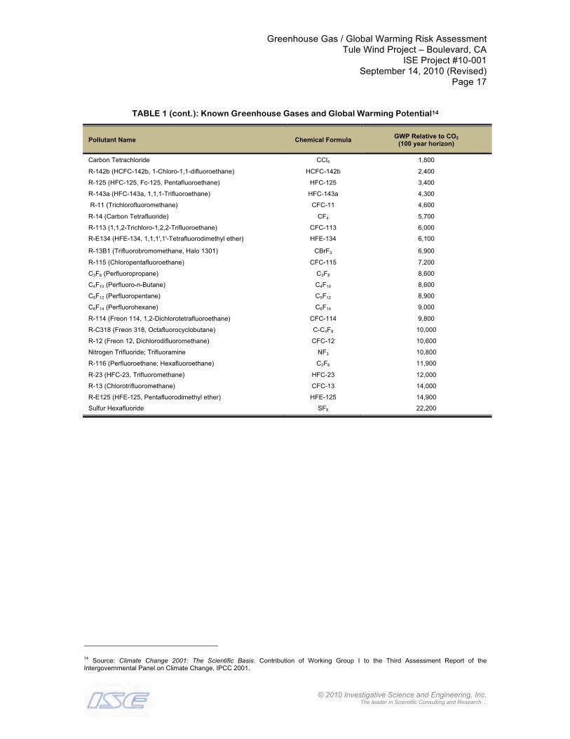
Greenhouse Gas / Global Warming Risk AssessmentTule Wind Project – Boulevard, CA
ISE Project #10-001September 14, 2010 (Revised)
Page 17
© 2010 Investigative Science and Engineering, Inc. The leader in Scientific Consulting and Research…
TABLE 1 (cont.): Known Greenhouse Gases and Global Warming Potential14
Pollutant Name Chemical Formula GWP Relative to CO2(100 year horizon)
Carbon Tetrachloride CCl4 1,800
R-142b (HCFC-142b, 1-Chloro-1,1-difluoroethane) HCFC-142b 2,400
R-125 (HFC-125, Fc-125, Pentafluoroethane) HFC-125 3,400
R-143a (HFC-143a, 1,1,1-Trifluoroethane) HFC-143a 4,300
R-11 (Trichlorofluoromethane) CFC-11 4,600
R-14 (Carbon Tetrafluoride) CF4 5,700
R-113 (1,1,2-Trichloro-1,2,2-Trifluoroethane) CFC-113 6,000
R-E134 (HFE-134, 1,1,1',1'-Tetrafluorodimethyl ether) HFE-134 6,100
R-13B1 (Trifluorobromomethane, Halo 1301) CBrF3 6,900
R-115 (Chloropentafluoroethane) CFC-115 7,200
C3F8 (Perfluoropropane) C3F8 8,600
C4F10 (Perfluoro-n-Butane) C4F10 8,600
C5F12 (Perfluoropentane) C5F12 8,900
C6F14 (Perfluorohexane) C6F14 9,000
R-114 (Freon 114, 1,2-Dichlorotetrafluoroethane) CFC-114 9,800
R-C318 (Freon 318, Octafluorocyclobutane) C-C4F8 10,000
R-12 (Freon 12, Dichlorodifluoromethane) CFC-12 10,600
Nitrogen Trifluoride; Trifluoramine NF3 10,800
R-116 (Perfluoroethane; Hexafluoroethane) C2F6 11,900
R-23 (HFC-23, Trifluoromethane) HFC-23 12,000
R-13 (Chlorotrifluoromethane) CFC-13 14,000
R-E125 (HFE-125, Pentafluorodimethyl ether) HFE-125 14,900
Sulfur Hexafluoride SF6 22,200
14 Source: Climate Change 2001: The Scientific Basis. Contribution of Working Group I to the Third Assessment Report of the Intergovernmental Panel on Climate Change, IPCC 2001.

Greenhouse Gas / Global Warming Risk AssessmentTule Wind Project – Boulevard, CA
ISE Project #10-001September 14, 2010 (Revised)
Page 18
© 2010 Investigative Science and Engineering, Inc. The leader in Scientific Consulting and Research…
THRESHOLDS OF SIGNIFICANCE
California Environmental Quality Act (CEQA) Thresholds
Section 15382 of the California Environmental Quality Act (CEQA) guidelines defines a significant impact as,
“… a substantial, or potentially substantial, adverse change in any of the physical conditions within the area affected by the project including land, air, water, minerals, flora, fauna, ambient noise, and objects of historic or aesthetic significance.”
Senate Bill 97 (2007) set a January 1, 2010, deadline for new CEQA guidelines related to greenhouse gas emissions analysis and mitigation.15 The new guidelines will require GHG emissions and their effects to be analyzed based on scientific and factual data.16 The new guidelines do not require CEQA to establish fixed thresholds of significance, rather they serve to update the procedural language of Section 15064(a)leaving individual significance criteria to local agencies.
The California Global Warming Solutions Act (AB 32) The California State Legislature, operating under the assumption that
anthropogenic global warming is a genuine phenomenon, and that atmospheric carbondioxide is the most significant contributor to this phenomenon, passed the California Global Warming Solutions Act of 2006 (AB 32). AB 32 requires the California Air Resources Board (CARB) to develop regulations and market mechanisms that will ultimately reduce California's greenhouse gas emissions by 25 percent by 2020. Mandatory caps will begin in 2012 for significant sources, and will incrementally become stricter to meet the 2020 goals.
Specifically, AB 32 requires CARB to:
1) Establish a statewide greenhouse gas emissions cap for 2020, based on 1990 emissions by January 1, 2008.
2) Adopt mandatory reporting rules for significant sources of greenhouse gases by January 1, 2009.
3) Adopt a plan by January 1, 2009 indicating how emission reductions will be achieved from significant greenhouse gas sources via regulations, market mechanisms and other actions.
4) Adopt regulations by January 1, 2011 to achieve the maximum technologically feasible and cost-effective reductions in greenhouse gas, including provisions for using both market mechanisms and alternative compliance mechanisms.
15 An act to add Section 21083.05 to, and to add and repeal Section 21097 of, the Public Resources Code, relating to the California Environmental Quality Act.16 This is consistent with all past and present ISE Greenhouse Gas / Global Warming Risk Assessments.

Greenhouse Gas / Global Warming Risk AssessmentTule Wind Project – Boulevard, CA
ISE Project #10-001September 14, 2010 (Revised)
Page 19
© 2010 Investigative Science and Engineering, Inc. The leader in Scientific Consulting and Research…
5) Convene an Environmental Justice Advisory Committee and an Economic and Technology Advancement Advisory Committee to advise CARB.
6) Ensure public notice and opportunity for comment for all CARB actions.
7) Prior to imposing any mandates or authorizing market mechanisms, CARB must evaluate several factors, including but not limited to, impacts on California's economy, the environment and public health; equity between regulated entities; electricity reliability; conformance with other environmental laws; and that the rules do not disproportionately impact low-income communities.
For the purposes of analysis within this report (and to be completely consistent with AB 32), it will be sought to; 1) quantify the aggregate greenhouse gas emissions due to the proposed project action, and, 2) quantify the net heating effect within the State of California.
CAPCOA Recommended CO2e Screening Levels The California Air Pollution Control Officers Association (CAPCOA) and CARB
currently publish CO2e screening levels for use in CEQA reporting. This screening level, set at 900 metric tons (i.e., 900 MT or 900,000 kilograms or 1,984,160 pounds) of CO2e
per year is ‘recommended’ for all new projects within the State of California for compliance with the intent of AB 32 as compared to ‘business as usual’.17
ISE utilizes the CAPCOA screening level for simple policy guidance purposeswithin the context of this report. Operational levels (or in this case construction worker trips) due to a proposed project action above the 900 MT screening value will be subject to additional recommendations for compliance per AB 32.
17 The CAPCOA whitepaper entitled, “CEQA & Climate Change – Evaluating and Addressing Greenhouse Gas Emissions from Projects Subject to the California Environmental Quality Act, January 2008” is very clear in its prefacing disclaimer that the proposed 900 MT screening level is not to be used for CEQA impact determination purposes. As stated in the document, “…This paper is intended as a resource, not a guidance document. It is not intended, and should not be interpreted, to dictate the manner in which an air district or lead agency chooses to address greenhouse gas emissions in the context of its review of projects under CEQA.” It should further be noted that the CAPCOA isn’t based upon any scientific analysis or rule-of-thumb, it is simply a screening level agreed to by various agencies within the State.

Greenhouse Gas / Global Warming Risk AssessmentTule Wind Project – Boulevard, CA
ISE Project #10-001September 14, 2010 (Revised)
Page 20
© 2010 Investigative Science and Engineering, Inc. The leader in Scientific Consulting and Research…
ANALYSIS METHODOLOGY
Greenhouse Gas Compilation Approach
Diesel Powered (Compression Ignition) Equipment Contribution
Greenhouse gas emissions associated with diesel engine combustion from construction equipment will be assumed to occur for engines running at the correct fuel to air ratios.18 Of principal interest are the emission factors for CO2 and NOX
19. For a four-
stroke diesel-cycle engine, the combustion byproducts are approximately 1.5-percent-by-volume O2, 0.5-percent-by-volume CO, and 13.5-percent-by-volume CO2.20 Thus, the ratio of CO2 to CO production in a properly mixed diesel stroke would be 13.5/0.5 or 27:1.
Construction Worker Motor Vehicle (Spark Ignition) Contribution
CARB estimates on-road motor vehicle emissions by using a series of models called the Motor Vehicle Emission Inventory (MVEI) Models. The four computer models, which form the MVEI, are CALIMFAC, WEIGHT, EMFAC, and BURDEN.21 For the current analysis, the EMFAC 2007 Model v2.3 of the MVEI22 was run using input conditions specific to the San Diego air basin to predict vehicle emissions based upon a worst-case year 2012 project initiation date.23 The aggregate greenhouse emission factors from the CARB EMFAC 2007 model are provided as an attachment to this report.Of principal interest are the emission factors for CO2 and NOX.
A mix ratio consistent with the Caltrans ITS Transportation Project-Level Carbon Monoxide Protocol was used. This consisted of the following air standard Otto-Cycle engine vehicle distribution percentages: Light Duty Autos (LDA) = 69.0%, Light Duty Trucks (LDT) = 19.4%, Medium Duty Trucks (MDT) = 6.4%, Heavy Duty Trucks (HDT) =4.7%, Buses (UBUS) = 0.0% and Motorcycles (MCY) = 0.5%.
18 The ratio whereby complete combustion of the diesel fuel occurs.19 It will be assumed that the project would generate trace-, if not negligible-, levels of methane (CH4), ozone (O3), fluorine (F2), chlorine (Cl2), bromine (Br2) and/or constituent compounds. NOx emissions are stoichiometrically composed of roughly 30-percent nitrous oxide (N2O) by volume and 70-percent nitric oxide (NO), which is the free radical form that immediately combines with ozone (O3) to form nitrogen dioxide (NO2) more commonly known as smog.20 Source: Holtz, J.C., Elliott, M.A., The Significance of Diesel-Exhaust-Gas Analysis, Transactions of the ASME, Vol. 63, February 1941. 21 CALIMFAC produces base emission rates for each model year when a vehicle is new, and as it accumulates mileage and the emission controls deteriorate. WEIGHT calculates the relative weighting each model year should be given in the total inventory, and each model year's accumulated mileage. EMFAC uses these pieces of information, along with the correction factors and other data, to produce fleet composite emission factors. BURDEN combines the emission factors with county-specific activity data to produce to emission inventories.22 This is the most current CARB vehicle emissions model approved for use within the State of California. Any subsidiary program (such as the previously discussed URBEMIS program) uses this model to determine the applicable vehicle emission factors.23 This is a worst-case assumption, since implementation of cleaner vehicle controls ultimately reduces emissions under future year conditions. By applying near-term emission factors to the complete project, an upper bound on project-related emissions is obtained.

Greenhouse Gas / Global Warming Risk AssessmentTule Wind Project – Boulevard, CA
ISE Project #10-001September 14, 2010 (Revised)
Page 21
© 2010 Investigative Science and Engineering, Inc. The leader in Scientific Consulting and Research…
Projected Greenhouse Gas Emissions Budget and Warming Effects Analysis
To address the net greenhouse gas emissions and perceived global warming potential of the project per AB 32, the entire State of California will be modeled as a thermodynamically closed system, subject only to increasing CO2 concentrations and their equivalents (denoted as CO2e).24 This approach creates a type of Urban Heat Islanddependant only on CO2e, whereby the effective temperature increase on the State due to the proposed project action can be quantified using the exact methodology identified in the U.N.’s Third Assessment Report of the IPCC.25
The analysis presented herein is consistent and in accordance with the First Law of Thermodynamics and the intent of AB 32.26 Mitigation measures consistent with the State of California’s policy implementation of AB 32 will be provided at the end of the report. FINDINGS
Greenhouse Gas Emission Tabulation
Diesel Powered (Compression Ignition) Equipment Contribution
The Tule Wind Project would utilize a worst-case contingency of equipment required to grade and prepare the site for a period of 576-days (i.e., a total of 192-days per each of the following phases: rough grading / tower pad work, underground utility construction / tower foundation work, and actual tower construction / finish work).27
Previous analysis of the required equipment and subsequent emissions budget has been examined within the project’s Air Quality Conformity Assessment.28 The pertinent findings are shown below, in Table 2.
24 Since the California legislature’s concern about the possible contribution of human activities to global warming was the impetus for the AB-32 legislation, and since this bill incorporates statewide reductions in greenhouse gas emissions to attempt to combat this potential issue, thorough discussions of both greenhouse gas emissions and global warming risk potential must be included in any complete report on the subject. 25 An Urban Heat Island (or UHI) is a developed area that is significantly warmer than its undeveloped surroundings. The temperature difference usually is larger at night than during the day, and larger in winter than in summer, due to the re-radiation of solar energy by paved surfaces and buildings, and waste heat generated by energy usage and building heating and cooling. Water vapor will be completely ignored from the analysis (as is done in the United Nations source document).26 Simply expressed, the First Law of Thermodynamics states that for any thermodynamic system, the sum of the heat ‘h’ contained within the system (or that it receives), plus the work ‘w’ that the system is capable of (or receives) is equal to the total internal energy ‘E’ of the system. The first law of thermodynamics basically states that a thermodynamic system can store energy in two different forms (namely heat and/or work) and that this internal energy is conserved.27 The analysis of GHG emissions, unlike air quality conformity, which is a ‘per day’ threshold, is an aggregate quantity requiring summation over the total estimated number of work days (i.e., the total number of days that any construction grading vehicle would have an engine running).28 Source: Air Quality Conformity Assessment – Tule Wind Project – Boulevard, CA, ISE Project #10-001, Investigative Science and Engineering, Inc., 9/14/10 (Revised).
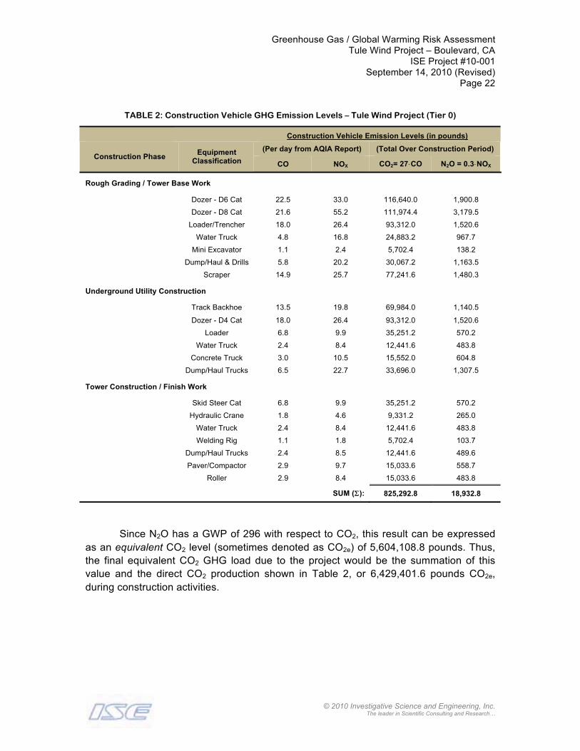
Greenhouse Gas / Global Warming Risk AssessmentTule Wind Project – Boulevard, CA
ISE Project #10-001September 14, 2010 (Revised)
Page 22
© 2010 Investigative Science and Engineering, Inc. The leader in Scientific Consulting and Research…
TABLE 2: Construction Vehicle GHG Emission Levels – Tule Wind Project (Tier 0)
Construction Vehicle Emission Levels (in pounds)(Per day from AQIA Report) (Total Over Construction Period)
Construction Phase Equipment Classification CO NOX CO2= 27⋅CO N2O = 0.3⋅NOX
Rough Grading / Tower Base Work
Dozer - D6 Cat 22.5 33.0 116,640.0 1,900.8
Dozer - D8 Cat 21.6 55.2 111,974.4 3,179.5
Loader/Trencher 18.0 26.4 93,312.0 1,520.6
Water Truck 4.8 16.8 24,883.2 967.7
Mini Excavator 1.1 2.4 5,702.4 138.2
Dump/Haul & Drills 5.8 20.2 30,067.2 1,163.5
Scraper 14.9 25.7 77,241.6 1,480.3
Underground Utility Construction
Track Backhoe 13.5 19.8 69,984.0 1,140.5
Dozer - D4 Cat 18.0 26.4 93,312.0 1,520.6
Loader 6.8 9.9 35,251.2 570.2
Water Truck 2.4 8.4 12,441.6 483.8
Concrete Truck 3.0 10.5 15,552.0 604.8
Dump/Haul Trucks 6.5 22.7 33,696.0 1,307.5
Tower Construction / Finish Work
Skid Steer Cat 6.8 9.9 35,251.2 570.2
Hydraulic Crane 1.8 4.6 9,331.2 265.0
Water Truck 2.4 8.4 12,441.6 483.8
Welding Rig 1.1 1.8 5,702.4 103.7
Dump/Haul Trucks 2.4 8.5 12,441.6 489.6
Paver/Compactor 2.9 9.7 15,033.6 558.7
Roller 2.9 8.4 15,033.6 483.8
SUM (Σ): 825,292.8 18,932.8
Since N2O has a GWP of 296 with respect to CO2, this result can be expressed as an equivalent CO2 level (sometimes denoted as CO2e) of 5,604,108.8 pounds. Thus, the final equivalent CO2 GHG load due to the project would be the summation of this value and the direct CO2 production shown in Table 2, or 6,429,401.6 pounds CO2e, during construction activities.
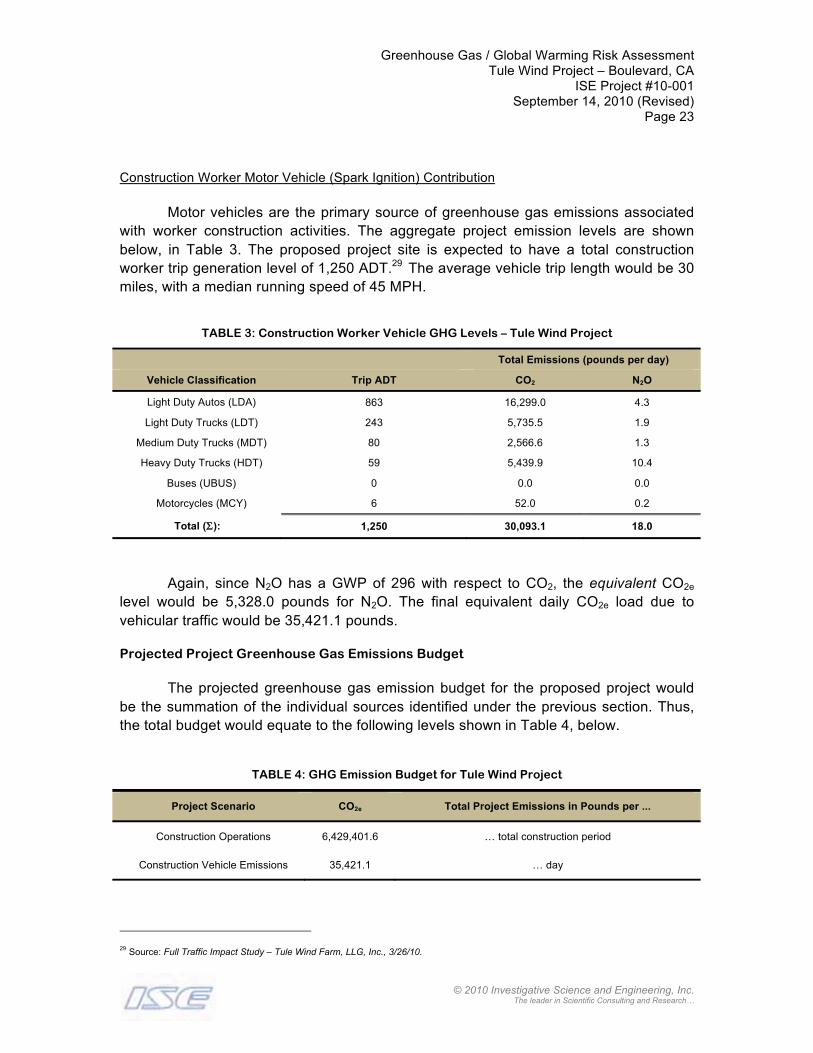
Greenhouse Gas / Global Warming Risk AssessmentTule Wind Project – Boulevard, CA
ISE Project #10-001September 14, 2010 (Revised)
Page 23
© 2010 Investigative Science and Engineering, Inc. The leader in Scientific Consulting and Research…
Construction Worker Motor Vehicle (Spark Ignition) Contribution
Motor vehicles are the primary source of greenhouse gas emissions associated with worker construction activities. The aggregate project emission levels are shown below, in Table 3. The proposed project site is expected to have a total construction worker trip generation level of 1,250 ADT.29 The average vehicle trip length would be 30miles, with a median running speed of 45 MPH.
TABLE 3: Construction Worker Vehicle GHG Levels – Tule Wind Project
Total Emissions (pounds per day)
Vehicle Classification Trip ADT CO2 N2O
Light Duty Autos (LDA) 863 16,299.0 4.3
Light Duty Trucks (LDT) 243 5,735.5 1.9
Medium Duty Trucks (MDT) 80 2,566.6 1.3
Heavy Duty Trucks (HDT) 59 5,439.9 10.4
Buses (UBUS) 0 0.0 0.0
Motorcycles (MCY) 6 52.0 0.2
Total (ΣΣ): 1,250 30,093.1 18.0
Again, since N2O has a GWP of 296 with respect to CO2, the equivalent CO2e
level would be 5,328.0 pounds for N2O. The final equivalent daily CO2e load due to vehicular traffic would be 35,421.1 pounds.
Projected Project Greenhouse Gas Emissions Budget
The projected greenhouse gas emission budget for the proposed project would be the summation of the individual sources identified under the previous section. Thus, the total budget would equate to the following levels shown in Table 4, below.
TABLE 4: GHG Emission Budget for Tule Wind Project
Project Scenario CO2e Total Project Emissions in Pounds per ...
Construction Operations 6,429,401.6 … total construction period
Construction Vehicle Emissions 35,421.1 … day
29 Source: Full Traffic Impact Study – Tule Wind Farm, LLG, Inc., 3/26/10.

Greenhouse Gas / Global Warming Risk AssessmentTule Wind Project – Boulevard, CA
ISE Project #10-001September 14, 2010 (Revised)
Page 24
© 2010 Investigative Science and Engineering, Inc. The leader in Scientific Consulting and Research…
The total aggregate construction GHG emissions would be 6,429,401.6 pounds CO2e. The total construction vehicle GHG emissions would be 35,421.1 pounds of equivalent CO2e per day. Thus, the total emissions would be expressed as 6,429,401.6 + 35,421.1/day pounds of CO2e. The total time duration would be at least two years, which is consistent with the proposed construction plan.
The vehicular CO2e level would be approximately 6.5 times greater than the CAPCOA 900 MT screening level due to project operation. It will be noted shortly, however, that the proposed project is nonetheless consistent with the intent of AB 32 due to its nature.
Projected Warming Effects Due to Project Equivalent CO2e
Finally, since AB 32 is formally known as the California Global Warming Solutions Act, it is of scientific interest to identify the level of warming predicted by construction and operation of the proposed project action and its effect on the State of California in terms of theoretical heating and the time for the project to manifest as any appreciable climate change according the U.N.’s Third Assessment Report of the IPCC.30
Given this, the proposed Tule Wind Project would contribute a construction vehicular total of 35,421.1 pounds of CO2e per day. Assuming all CO2e mixing occurs within the Troposphere31, the thermodynamic system consisting of the boundaries of the State of California would have a volume32 of,
VsystemCalifornia
= 104,765,440 acres ×43,560 sq-ft
acre× 37,000 ft = 1.6884x1017 ft3
Since one part-per-million-by-volume (ppmv) of CO2 equals 1.12315x10⁻⁷
pounds-per-cubic-foot at Standard Temperature and Pressure (STP), the daily increasein CO2e concentration due to the proposed project action within the State of California would be,
COConcSystem=
35,421.1 pounds1.6884x1017 ft3 ×
1 ppmv CO2
1.12315x10⁻⁷ poundsft3 @STP
= 1.87x10⁻⁶ ppmv/day
30 This is, of course, the entire point behind the legislative mandate of AB 32, namely to reduce the global warming effects produced by the State of California. 31 The troposphere is the lowest portion of Earth's atmosphere and contains approximately 75% of the atmospheric mass of the planet and almost all of its water vapor and GHG’s. The average depth of the troposphere is approximately seven miles (≈37,000 feet). For the purposes of analysis we will assume that all mixing occurs at sea level (which produces the greatest atmospheric concentrations and subsequent radiative forcing).32 The area within the State of California is approximately 163,696 square miles (104,765,440 acres) which, when multiplied by the height of the tropopause, roughly equates to 1.6884x1017 ft3. This is also the jurisdictional boundary of AB 32.

Greenhouse Gas / Global Warming Risk AssessmentTule Wind Project – Boulevard, CA
ISE Project #10-001September 14, 2010 (Revised)
Page 25
© 2010 Investigative Science and Engineering, Inc. The leader in Scientific Consulting and Research…
This equates to a 0.00000187 ppmv/day CO2e increase within our troposphericsystem bounded by the land mass limits of the State of California. Given this, the yearly concentration increase in CO2e due to the proposed project action would be 0.0006817ppmv/year. Substituting the previously cited construction total from above, it can similarly be shown that the aggregate concentration due to the totality of construction would be 0.00033903 ppmv to our system.
Thus, we can rewrite our CO2e forcing function in terms of the number of elapsed years (Δyr ) from the start of construction of the project as:
Conc. CO2e /yr = 0.00033903 ppmv + 0.0006817 ppmv/yr= 0.00033903 + 0.0006817(Δyr) (in ppmv)
The net change in radiative forcing due to a change in CO2e is defined within the IPCC report33 as,
ΔF = α Ln CC0
⎛⎝⎜
⎞⎠⎟
where, ΔF is the change in the radiative forcing (in W/m2), α is the atmospheric forcing coefficient = 5.35, 34
C is the baseline plus project CO2 and CO2e concentrations (in ppmv), and, C0 is the baseline CO2 concentration (commonly taken as 380 ppmv).
Furthermore, surface air temperature sensitivity factors cited by the IPCC have a global average of approximately 0.1 °C/W/m2. Thus, the net yearly increase in temperature for the first year of operation due to the proposed project CO2e emissions would be,
ΔTProject(year= 1) = 0.1o C
W/m2 × 5.35Ln 380 + 0.00033903 + 0.0006817(Δyr)380
⎛⎝⎜
⎞⎠⎟W
m2
= 0.1o C
W/m2 × 5.35Ln 380 + 0.00033903 + 0.0006817(1)380
⎛⎝⎜
⎞⎠⎟W
m2
= 3.7730x10⁻⁷ oC
33 Source: Third Assessment Report of Working Group I of the Intergovernmental Panel on Climate Change (IPCC), 2001.34Based on carbon dioxide contributing approximately 32 watts per square-meter (W/m2) of long-wave radiative forcing to the climate system under a clear-sky condition, out of a total of 125 watts per square-meter for all atmospheric gases under the same conditions. The total radiative forcing from the Sun as of 1997 was 342 W/m2.

Greenhouse Gas / Global Warming Risk AssessmentTule Wind Project – Boulevard, CA
ISE Project #10-001September 14, 2010 (Revised)
Page 26
© 2010 Investigative Science and Engineering, Inc. The leader in Scientific Consulting and Research…
Since the proposed Tule Wind Project would produce worker vehicle trips for the estimated two active years of construction, and possibly a third year for finalization of the project, the resultant worst-case temperature increase to the State of California would be,
ΔTProject(year= 1) = = 0.1o C
W/m2 × 5.35Ln 380 + 0.00033903 + 0.0006817(3)380
⎛⎝⎜
⎞⎠⎟W
m2
= 3.3567x10⁻⁶ oC
Finally, remembering that the above expression is logarithmic in nature, one could iterate the above solution to determine the time required for the Tule Wind Projectto increase the temperature within the State of California one degree Centigrade under the worst-case closed-system condition and perpetual traffic levels equal to the construction averages. This one-degree-Centigrade increase due to the proposed project under consideration would occur in approximately 3,058,390 years.35
CONCLUSIONS / RECOMMENDATIONS
Project-Related Greenhouse Gas Budget / Global Warming Potential
The proposed Tule Wind Project site was shown to produce an aggregate equivalent greenhouse gas loading of 6429401.6 + 35421.1/day pounds of CO2e. The local annual warming effect due to this level of project emissions was found to be 3.3567x10⁻⁶ °C, which would be deemed as cumulatively considerable and mitigable under CEQA. The net contribution to planet Earth as a whole would be deemed insignificant.36
Compliance with AB 32 CO2 Reduction Strategies
Since the project provides a clean inexhaustible source of electricity that reduces the dependence of the State of California on imports of natural gas, oil, and other fuels, it is, by definition consistent with the intent of AB 32 and the California Renewable Portfolio Standard Program. The near term and future benefits of the project far outweigh any air pollution and global warming required for its construction. As a result, no additional compliance measures under AB 32 are required.
35 The one-degree Centigrade point is the current threshold discussed in the scientific literature whereby a perceivable change in the affected environment is expected. As can be seen, the proposed project would produce an extremely small, but measurable change in the affected environment following the IPCC’s scientific model. 36 Ninety-percent (90%) of the atmosphere of the planet Earth resides within 16 kilometers (16,000 meters) of the surface. Thus, the volume of the atmosphere is roughly 8.2x10⁹ km3 (8.2x10¹⁸ m3 or 2.9x1020 ft3). The mass of the atmosphere is roughly 5.3x10²¹ grams or 1.17x10¹⁹
pounds. Although the project’s contribution is mathematically a finite number, it is also asymptotically driven to zero in its bounded limit. Thus, the net temperature contribution of the proposed project to the planet as a whole is physically zero, and in fact could not even be directly measured using modern scientific instrumentation.

Greenhouse Gas / Global Warming Risk AssessmentTule Wind Project – Boulevard, CA
ISE Project #10-001September 14, 2010 (Revised)
Page 27
© 2010 Investigative Science and Engineering, Inc. The leader in Scientific Consulting and Research…
CERTIFICATION OF ACCURACY AND QUALIFICATIONS
This report was prepared by Investigative Science and Engineering, Inc. (ISE), located at 1134 D Street, Ramona, CA 92065. The members of its professional staff contributing to the report are listed below:
Rick Tavares Ph.D. Civil Engineering([email protected]) M.S. Structural Engineering
M.S. Mechanical EngineeringB.S. Aerospace Engineering / Engineering Mechanics
Karen Tavares B.S. Electrical Engineering([email protected])
ISE affirms to the best of its knowledge and belief that the statements and information contained herein are in all respects true and correct as of the date of this report. Should the reader have any questions regarding the findings and conclusions presented in this report, please do not hesitate to contact ISE at (760) 787-0016.
Content and information contained within this report is intended only for the subject project and is protected under 17 U.S.C. §§ 101 through 810. Original reports contain a non-photo blue ISE watermark at the bottom of each page.
Approved as to Form and Content:
Rick Tavares, Ph.D.
Project PrincipalInvestigative Science and Engineering, Inc. (ISE)

Greenhouse Gas / Global Warming Risk AssessmentTule Wind Project – Boulevard, CA
ISE Project #10-001September 14, 2010 (Revised)
Page 28
© 2010 Investigative Science and Engineering, Inc. The leader in Scientific Consulting and Research…
APPENDICES / SUPPLEMENTAL INFORMATION
EMFAC 2007 EMISSION FACTOR TABULATIONS – SCENARIO YEAR 2012
Title : San Diego County Subarea Winter CYr 2012Version : Emfac2007 V2.3 Nov 1 2006Run Date : 2010/02/16 17:39:27Scen Year: 2012 -- All model years in the range 1968 to 2012 selectedSeason : WinterArea : San Diego***************************************************************************************** Year: 2012 -- Model Years 1968 to 2012 Inclusive -- Winter Emfac2007 Emission Factors: V2.3 Nov 1 2006
County Average San Diego County Average
Table 1: Running Exhaust Emissions (grams/mile)
Pollutant Name: Oxides of Nitrogen Temperature: 50F Relative Humidity: 40%
Speed MPH LDA LDT MDT HDT UBUS MCY ALL
10 0.391 0.616 1.095 15.228 23.752 1.320 1.162 15 0.348 0.542 0.973 11.723 19.230 1.321 0.960 20 0.316 0.488 0.888 10.139 16.369 1.333 0.851 25 0.292 0.448 0.831 9.557 14.638 1.353 0.795 30 0.274 0.420 0.795 9.148 13.742 1.381 0.756 35 0.263 0.402 0.779 8.899 13.534 1.415 0.733 40 0.256 0.392 0.779 8.809 13.978 1.456 0.724 45 0.253 0.391 0.796 8.884 15.139 1.504 0.729 50 0.255 0.397 0.833 9.140 17.200 1.558 0.750 55 0.262 0.411 0.891 9.610 20.512 1.618 0.788 60 0.273 0.435 0.977 10.343 25.694 1.687 0.848 65 0.290 0.471 1.102 11.419 33.832 1.765 0.938
Pollutant Name: Carbon Dioxide Temperature: 50F Relative Humidity: 40%
Speed MPH LDA LDT MDT HDT UBUS MCY ALL
10 715.721 891.565 1248.004 2301.762 2476.251 209.611 899.142 15 561.473 700.022 965.645 1947.099 2379.933 180.835 710.043 20 457.167 570.499 779.688 1700.690 2321.286 159.834 582.541 25 386.346 482.554 656.013 1601.083 2284.838 144.745 498.877 30 338.862 423.590 574.421 1524.761 2262.131 134.357 442.584 35 308.464 385.843 522.858 1467.236 2248.467 127.929 406.305 40 291.417 364.674 494.303 1426.052 2241.275 125.090 385.672 45 285.724 357.605 485.087 1400.000 2239.289 125.795 378.368 50 290.736 363.829 494.072 1388.756 2242.172 130.345 383.653 55 307.025 384.056 522.410 1392.791 2250.415 139.466 402.213 60 336.494 420.649 573.795 1413.505 2265.484 154.471 436.304 65 382.749 478.088 655.314 1453.648 2290.258 177.560 490.213
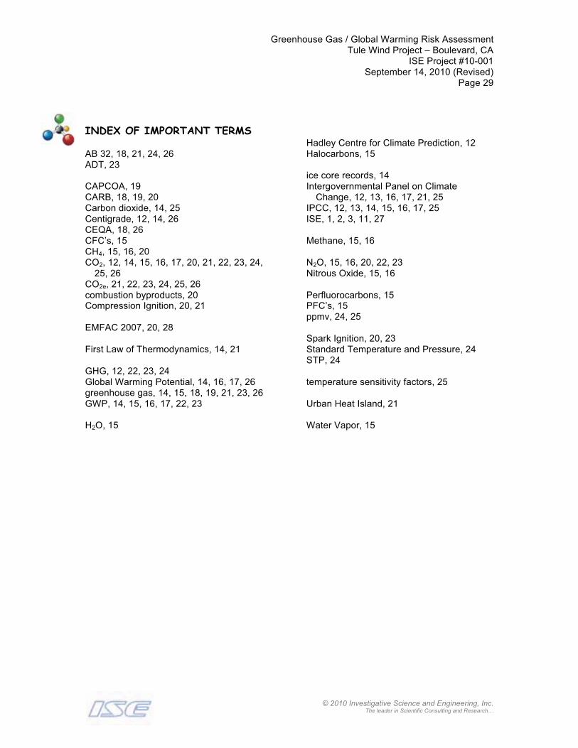
Greenhouse Gas / Global Warming Risk AssessmentTule Wind Project – Boulevard, CA
ISE Project #10-001September 14, 2010 (Revised)
Page 29
© 2010 Investigative Science and Engineering, Inc. The leader in Scientific Consulting and Research…
INDEX OF IMPORTANT TERMS
AB 32, 18, 21, 24, 26ADT, 23
CAPCOA, 19CARB, 18, 19, 20Carbon dioxide, 14, 25Centigrade, 12, 14, 26CEQA, 18, 26CFC’s, 15CH4, 15, 16, 20CO2, 12, 14, 15, 16, 17, 20, 21, 22, 23, 24,
25, 26CO2e, 21, 22, 23, 24, 25, 26combustion byproducts, 20Compression Ignition, 20, 21
EMFAC 2007, 20, 28
First Law of Thermodynamics, 14, 21
GHG, 12, 22, 23, 24Global Warming Potential, 14, 16, 17, 26greenhouse gas, 14, 15, 18, 19, 21, 23, 26GWP, 14, 15, 16, 17, 22, 23
H2O, 15
Hadley Centre for Climate Prediction, 12Halocarbons, 15
ice core records, 14Intergovernmental Panel on Climate
Change, 12, 13, 16, 17, 21, 25IPCC, 12, 13, 14, 15, 16, 17, 25ISE, 1, 2, 3, 11, 27
Methane, 15, 16
N2O, 15, 16, 20, 22, 23Nitrous Oxide, 15, 16
Perfluorocarbons, 15PFC’s, 15ppmv, 24, 25
Spark Ignition, 20, 23Standard Temperature and Pressure, 24STP, 24
temperature sensitivity factors, 25
Urban Heat Island, 21
Water Vapor, 15
