NOAA Technical Memorandum NMFS-AFSC-109

U.S. DEPARTMENT OF COMMERCENational Oceanic and Atmospheric Administration

National Marine Fisheries ServiceAlaska Fisheries Science Center

November 1999

byC. W. Fowler and M. A. Perez

Constructing Species FrequencyDistributions - A Step TowardSystemic Management

NOAA Technical Memorandum NMFS

The National Marine Fisheries Service's Alaska Fisheries Science Center uses theNOAA Technical Memorandum series to issue informal scientific and technicalpublications when complete formal review and editorial processing are notappropriate or feasible. Documents within this series reflect sound professionalwork and may be referenced in the formal scientific and technical literature.

The NMFS-AFSC Technical Memorandum series of the Alaska Fisheries ScienceCenter continues the NMFS-F/NWC series established in 1970 by the NorthwestFisheries Center. The new NMFS-NWFSC series will be used by the NorthwestFisheries Science Center.

This document should be cited as follows:

Fowler, C. W., and M. A. Perez. 1999. Constructing species frequencydistributions - a step toward systemic management. U.S. Dep. Commer.,NOAA Tech. Memo. NMFS-AFSC-109, 59 p.

Reference in this document to trade names does not imply endorsement by theNational Marine Fisheries Service, NOAA.

Notice to Users of this Document

In the process of converting the original printed document into an Adobe,PDF format, slight difference informatting occur. The material presented in the original printed document and this PDF version, however, is thesame.

This document is available to the public through:

National Technical Information Service

U.S. Department of Commerce

52885 Port Royal Road

Springfield, VA 22161

www.ntis.gov

November 1999

NOAA Technical Memorandum NMFS-AFSC-109

byC. W. Fowler and M. A. Perez

Constructing Species FrequencyDistributions - A Step Toward

Systemic Management

National Marine Mammal LaboratoryAlaska Fisheries Science Center

7600 Sand Point Way N.E., BIN C-15700Seattle, WA 98115-0070

U.S. DEPARTMENT OF COMMERCEWilliam M. Daley, Secretary

National Oceanic and Atmospheric AdministrationD. James Baker, Under Secretary and Administrator

National Marine Fisheries ServicePenelope D. Dalton, Assistant Administrator for Fisheries

iii

Abstract

There is practical importance to understanding the process ofconstructing frequency distributions for the characteristics of species.Such distributions represent diversity and are needed to measure andobserve the limits to variation among species so that such informationcan be used in management. Basically, the construction of speciesfrequency distributions involves four steps: 1) data collection(measuring species); 2) finding the range of values within the data(maximum minus minimum); 3) subdivision of the range intocategories or bins; 4) finding the portion of species that fall in eachcategory established in step 3 (i.e., fraction of the sample of speciesmeasured); and 4) plotting the results in a histogram to produce agraphic representation of an underlying probability distribution.Various measures of species are possible and can be represented insuch distributions to depict variation and its limits. Examples arechromosome count, population variation, geographic range size, carbondioxide production, biomass consumption, and mean adult body mass.Management depends on such measures so that efforts can be made,where possible, to keep species within the normal range of naturalvariation in order to implement one of the primary principles ofmanagement.

v

ContentsPage

Introduction ............................................................................................................................. 1

Frequency Distributions .......................................................................................................... 1

Basic Steps - Raw data ............................................................................................... 2

Transformed Data ....................................................................................................... 2

Terrestrial Mammal Example .................................................................................... 4

Measures of Species ................................................................................................................ 6

Simple or Direct Measures.......................................................................................... 6

Population variation ..................................................................................... 6

Population size .............................................................................................. 8

Geographic range .......................................................................................... 9

Chromosome count ..................................................................................... 10

Derived Species-level Measures............................................................................... 12

Carbon dioxide production ......................................................................... 12

Energy consumption ................................................................................... 12

Consumption of biomass from ecosystems ................................................ 14

Consumption of biomass from individual prey species .............................. 16

Bivariate Space ..................................................................................................................... 17

More Complex Correlations ................................................................................................. 21

Use of Species Frequency Distributions ............................................................................... 22

Summary ............................................................................................................................... 26

Acknowledgments ................................................................................................................. 27

Citations ................................................................................................................................ 29

Appendix ............................................................................................................................... 31

)))))))))) Introduction ))))))))))

There is a great deal o f variation among species

with regard to mean adult body size, biomass

consumption, geographic range size, carbon dioxide

production, population size and other characteristics

that can be measured or estimated. This diversity

exhibits limits, however, and both variation and its

limits are of practical importance. To derive useful

information from the measure of species, data must be

collected, analyzed and displayed.

This docume nt presents the basic processes

underlying the graphic and quantitative presentation of

variation among species. We begin by describing the

general process o f building the p robability distributions

that represent various collections of species - what we

call simple species frequency distributions. Then we

proceed to generate more complex distributions using

both observed and derive d data . Finally, we briefly

discuss the use of spe cies frequen cy distributions in

managem ent.

In general, varia bility can be sho wn in histograms

(bar graphs), whether it is for body tem perature, ra in

fall, or seed numbers (e.g., see Schmid 1 983). Similar

displays can be co nstructed for measures tha t apply to

species (e.g., mean adult body size, population size,

populati on variation, or rate of increase in population

numbers). Thus, histograms show variation among

species as a graphic presentation of what statisticians

call dispersion. However, it is important to recognize

that variability is constrained and that frequency

distributions also demonstrate these limits as well as

the resulting central tende ncies or agg regations. In this

paper, we present part of the analytic mechanics

needed to make such inform ation availab le for use in

management. Management based on information about

the limits to variation among species (Fowler 1999,

Fowler et al. 1999, Fowler unpub. m anuscript) wo uld

replace present approaches (e.g., single-species

approaches) to include applications for ecosystems and

the biosph ere. This form of management is discussed

at the end of this d ocumen t where we in dicate that it

would make direct use of such information to ensure

that human influences within ecosystems and the

biosphere would fall within the normal ranges of

observed natural variation among species. In the next

section, we describe the construction of species

frequency distributions as o bserved p robability

distributions of species-level traits (e.g., Fowler 1999,

Fowler et al. 1999, Fowler unpub. manuscript). They

are often shown graphically in histograms (bar graphs)

to visually demonstrate the central tendencies, limits,

and other statistical properties of variation among

species. Such distributions are an integration of the

factors that influence the measurements o f species by

reflecting all of the influential elemen ts that determine

where each species falls within the distribution.

We have concentrated on the production of

graphic presentations using both observed and derived

data. Mathematical models of frequency distributions

(normal distributions, log normal distrib utions, etc.;

Christensen 1984) c an also be fit to su ch data to

provide quantitative d escriptions as proba bility

distributions. Such analytic treatment, however, is

beyond the scope of this paper.

)))))))))) Frequency Distributions ))))))))))

In this section, we describe the general process of

presenting frequency distributions as they ap ply to

species. After describ ing frequenc y distributions

themselves, we demonstrate this process using raw data

for the body size of marine mammals. We then repeat

the process after applying a transformation to the data.

We also provide a second example that makes use of

data for the bod y size of terrestrial mamma ls, again

proceeding from raw to transformed data.

Statistically, a frequency distribution presents the

distribution of a variable in a way that illustrates b oth

its limits (constraints on its dispersion) and its central

tendencies (location in the spectrum of real numbers

toward which variatio n is constrained ). It represents

measurements from a pro bability distribu tion

characteris tic of natural systems being measured,

including measurement error.

The general concept of freque ncy distributions and

their construction is described in most elementary

statistical texts (e.g., Dixon and Massey 1957,

Huntsberger 1961, A lder and Roessler 1964) and

books on graphic presentation of data (e .g., Schmid

1983). One product of the process of constructing

frequency distributions is a histogram (bar graph) as a

2

graphic presentation commonly found in elementary

texts for such things as rainfall (Alder and Roessler

1964), grain production (Huntsberger 1961), age

(referred to as an age distribution within a population,

Schmid 1983), or the height of individual humans

(Dixon and Massey 1957). In the following

paragraphs, we review the general process by way of

example, then we proceed to a consideration of types of

measurem ents that apply to species and conclude with

other examples of spe cies frequency distributions.

Basic steps - raw data

The first step in constructing a frequency

distribution is the collection of data, either from

original research o r from published literature. For

example, columns E and H of Appendix T able 1 are

lists of values resulting from the m easureme nt of a

variable: in this case the mean adult body mass (kg) of

103 species of m arine mam mals. At the species level,

these values exemplify raw data or original

measurements. In this particular case the data were

collected from the pub lished literature (A ppendix

Table 1, Column B), which, of course, is based on field

research conducted over a long history of studies by

many researchers and measurements of individual

organisms.

The second step in producing a frequency

distribution is the analytic step of finding the range of

the data: the difference between the maximum and the

minimum of observe d measure ments. In this case, the

difference is about 150,000 kg: Maximum (M ax) =

150,000 kg, Minimum (Min) = 27.2 kg (Max-Min =

range = 149,972.8 kg, Appendix T able 1).

The third step is that of d ividing this range of

observed values into convenient increments, or

categories, often called bins. For graphic presentation,

it is often useful to p ick between 5 and 50 (usually 10-

20) bins. Here, we choose to use 20. If need ed (e.g.,

for comparison or observing change), empty bins can

be added above or below the range covered by the data.

The size range of each individual bin is first

approximated by dividing the range by the number of

bins. For our example (using the rounded range size),

the bin size would be 150,000/20 or 7,500 kg. For

convenience, this value can also be rounde d and we use

10,000 kg for this example where 10,000 kg is now the

increment from each bin's lower bound to its upper

bound. The lower bound of the first bin must be less

than the minimum of the data. Here, we s elected 0.0

kg, which is smaller than the minimum of 27.2 kg, the

adult body mass of sea o tters (Enhyd ra lutris).

Next, the values of the raw data (i.e., those of

columns E and H , Append ix Table 1 ) are assigned to

each bin as coun ts. Thus, for our example, we count 93

species for which me asured bo dy size falls in the first

bin (i.e., between a body s ize larger than 0.0 kg and

less than, or equal to, 10,000 kg, as arranged from the

top of column H in Appendix Table 1, in order by

size). Two were species assigned to the second bin

(species numbered 15 and 16 near the end of column H

in Append ix Table 1 ), and so forth , for the comp lete

range of data. The se counts are summarize d in

Table 1a (third column of the left section of Table 1).

To compar e between samples o f different sizes (i.e.,

different from the 103 species in this sample), the data

can be expressed in terms of the fraction (alternatively,

percent) of the overall sample. Thus, the 93 species

from the first bin comprise 0.903 (93/103 or 90.3%) of

the total of 103 species. Table 1a (fourth column)

presents these portions where, for example, the 2

species in the second bin were 1.9% of the total (2/103

= 0.019), and so forth, throu gh the entire series of bins.

The final graphic presentation of the resulting

frequency distribution is accomplished by drawing a

histogram (Fig. 1A) with data from the first and fourth

columns of Table 1a. The first column (alte rnatively

the second column or, better, a midpoint between the

upper and lower limits of the bins) provides the

measure used for the abscissa ( x-axis). The fourth

column provides the data to be plotted as the height of

the bars corre sponding to values shown on the ord inate

(y-axis). Additiona l bins can be added to the left

(lower) and right (upper) portions of the ab scissa to

meet the needs of individual applications (e.g., for

comparison with other data, as we will do below, or for

aesthetic purposes).

Transformed data

As can be seen from Figure 1A, the raw data of our

example are not normally distributed: there is an

extreme right skew to the data. In a normal

distribution, half the species would have had mean

body sizes above the mean of the distribution and half

below. Data such as those displayed in Figure 1A need

to be transformed to achieve a distribution that is closer

to normal. Here (as is often the case with species-level

measurements), a distribution that is normal (or more

nearly normal) can be achieved by using a log

transform - that is, by taking the logarithm (using

base 10, but any logarithmic base could be used) of

each value in columns E and H of Appendix Table 1.

These values are presented in columns F and I,

respectively, of Appendix Table 1. Other

transformations are useful and appropriate for other

kinds of data (e.g., arcsine for portions, Dixon and

Massey 1957, Huntsberger 1961, Alder and Roessler

1964).

3

Table 1. Data regarding body mass of 103 species of marine mammals from Append ix Table 1 consolid ated into

frequency distributions, both for the raw data (Table 1a) and log10 transformed data (Table 1b).

Table 1a Table 1b

Raw data (kg) Transformed data (log10(kg))

Bin sizeNumber

of species

Portion of

species

Bin sizeNumber

of species

Portion of

speciesfromto (and

including)from

to (and

including)

0 10,000 93 0.903 0.75 1.00 0 0.000

10,000 20,000 2 0.019 1.00 1.25 0 0.000

20,000 30,000 2 0.019 1.25 1.50 1 0.010

30,000 40,000 1 0.010 1.50 1.75 9 0.087

40,000 50,000 0 0.000 1.75 2.00 20 0.194

50,000 60,000 1 0.010 2.00 2.25 13 0.126

60,000 70,000 2 0.019 2.25 2.50 13 0.126

70,000 80,000 1 0.010 2.50 2.75 8 0.078

80,000 90,000 0 0.000 2.75 3.00 4 0.039

90,000 100,000 0 0.000 3.00 3.25 5 0.049

100,000 110,000 0 0.000 3.25 3.50 4 0.039

110,000 120,000 0 0.000 3.50 3.75 13 0.126

120,000 130,000 0 0.000 3.75 4.00 3 0.029

130,000 140,000 0 0.000 4.00 4.25 2 0.019

140,000 150,000 1 0.010 4.25 4.50 2 0.019

150,000 160,000 0 0.000 4.50 4.75 2 0.019

160,000 170,000 0 0.000 4.75 5.00 3 0.029

170,000 180,000 0 0.000 5.00 5.25 1 0.010

180,000 190,000 0 0.000 5.25 5.50 0 0.000

190,000 200,000 0 0.000 5.50 5.75 0 0.000

Figure 1.

The frequency distribution of

the adult body mass of 103

species of marine mamma ls

(data from Ta ble 1): Panel A

shows the distribution of the raw

data and Panel B shows the

d i s t r i b u t i o n a f t e r l o g 1 0

transformation of the same data.

4

The process described above can now be repeated

to achieve a graph using the transformed values. In

other words, the range is determ ined; this range is

subdivided into segments or bins (first and second

columns of Table 1b). The n the count o f values (i.e.,

next to last column of Table 1 b) is determined for each

bin and the portion of the sample in each bin is

calculated using the same procedures that were used for

the raw data (i.e., the last column of Table 1b was

determined by dividing the values in the next to last

column by the total number of species,1 03). Finally, a

corresponding graph is dra wn (Fig. 1B). Note the

continued presence of a right-handed skew, but one that

is much less extr eme than th at observed before the

transformation.

Terrestr ial mamm al examp le

Here, we repeat the steps described above using

the body mass (kg) of 368 species of terrestrial

mammals, starting with the information found in

Appendix Table 2 (Damuth 1987). Table 2

summarizes the data for the frequency distribution for

both the original measurements and after log10

transformation. As in the previous example, the values

presented in Table 2 resulted from finding the range of

data (both raw and transformed ) and divid ing it into

increments, then finding the count and portion of

species in each bin. Note that the bin sizes are

different from the previous example. The raw data for

marine mamma ls above we re divided into 10,000 kg

increments, whereas the terrestrial data were divided

into 200 kg increments. For the log10 transformed data,

the increments c orrespo nding to the bin size were 0.25

for marine mamma ls and 0.5 for terrestrial mammals.

The results for the sample of terrestrial mammals are

shown in Figure 2 based on the numerical information

in Table 2.

Table 2. Data rega rding bod y mass of 36 8 species o f terrestrial mam malian prim ary consum ers from Ap pendix

Table 2 consolidated into frequency distributions, both for the raw data (Table 2a) and log10 transformed data

(Table 2b).

Table 2a Table 2b

Raw data (kg) Transformed data (log10(kg))

Bin sizeNumber

of species

Portion of

species

Bin sizeNumber

of species

Portion of

speciesfromto (and

including)from

to (and

including)

0 200 343 0.932 -3.5 -3.00 0 0.000

200 400 11 0.030 -3.0 -2.50 0 0.000

400 600 5 0.014 -2.5 -2.00 8 0.022

600 800 0 0.000 -2.0 -1.50 32 0.087

800 1,000 4 0.011 -1.5 -1.00 77 0.209

1,000 1,200 1 0.003 -1.0 -0.50 47 0.128

1,200 1,400 1 0.003 -0.5 0.00 25 0.068

1,400 1,600 0 0.000 0.0 0.50 31 0.084

1,600 1,800 0 0.000 0.5 1.00 45 0.122

1,800 2,000 1 0.003 1.0 1.50 31 0.084

2,000 2,200 0 0.000 1.5 2.00 32 0.087

2,200 2,400 1 0.003 2.0 2.50 25 0.068

2,400 2,600 0 0.000 2.5 3.00 10 0.027

2,600 2,800 0 0.000 3.0 3.50 5 0.014

2,800 3,000 1 0.003 3.5 4.00 0 0.000

3,000 3,200 0 0.000 4.0 4.50 0 0.000

5

Figure 2.

The frequency distribution of

the adult body mass of the 368

species of terrestrial mammalian

primary consume rs from Ta ble

2 : Panel A shows th e

distribution of the raw data and

Panel B shows the distribution

after log10 transformation.

Figure 3.

A comparison of body mass

among marine (Panel A ) and

terrestrial (Panel B ) mamma ls

based on the log10 transformed

data from Figures 1 and 2.

Figure 3 shows a comparison of the distribution of

the adult bo dy size of ma rine and terre strial mamm als

as a compo site of Figures 1B and 2B. Several features

of these graphs are of note, each of which is necessary

to accomplish the com parison. First, bins contain ing

zeros have been added to the range of values for

marine mamma ls at the low end o f the scale (in

converting Fig. 1B to Fig. 3A). Other bins have been

6

added to the high end of the range used for terrestrial

species (converting Fig. 2B to Fig. 3B). Second, the

scales on both the x and y axes were made the same. In

part, this was accomplished by adding bins, as just

mentioned, but it also involved using the same bin size.

It is important that identical ranges and scales be used

to accommodate the comparison between the two

groups. The bin size used in this comparison was the

same as that chosen for the terrestrial species in

Figure 2B (i.e., 0.5 for the log transformation). And

third, each number among the labels used for the

abscissa represents the lower end of the range for the

corresponding bin that is depicted by the bar directly

above it. These numbers could have been either the

upper bound o r the midpo int of the range of each b in

and remained equally as useful. For quantitative

analysis, however, the use of mid points to define bins

is imperative (b ecause mid points are used as surrogates

for the raw data, multiplied by corresponding counts,

such that either the upper o r lower rang e limits would

result in bias of one-half the range size of each bin;

Dixon and Massey 1957, Huntsberger 1961, Alder and

Roessler 1964).

)))))))))) Measures of Species ))))))))))

The examples described above, and examples

provided in the general texts referred to above,

demon strate the general procedure for producing

frequency distributions. The data used in these

examples were representative of species-level

measurements. That is, the mean adult body masses

represent species-specific measurements. Note that

measurem ents of individuals were necessary to

calculate these means as species-level measurements.

Frequency distributions among individuals within a

species can be produced by the same process, and these

could be presented as individual-level frequency

distributions (one per species). T he species-level

measurem ents used in the examples for marine and

terrestrial mammals were the means of such

distributions among individuals from e ach species,

respectively.

Measu rements can be made of many other species-

level characteristics a nd the data for producing the

relevant distributions can be derived through two

processes. The first process involves direct

measurem ent, such as measuring body weight or mass

in the examples above, measures of total biomass, or

population variation. The second process involves

indirect measures to result in estimates of such

characteristics as carbon dioxide production or total

annual energy consumption. These indirect measures

are derived by the quantitative combination of separate

sets of related information. Other measures of species

include the numbers of species consumed as prey

(number of resource species) and the number of

consumer species for which a species serves as a

resource. Each measure can be portrayed in a species

frequency distribution such as those shown in Figures

1-3. Further demonstration of such measures will be

presented in the examples below.

Simple or direct measures

Calling measures of species "simple" minimizes

the difficulty of making measurements in field research.

The importan t concept h ere is that the me asuremen ts

are achieved less by inference than by direct

observation in field or laboratory research. Comparing

the set of examples in this section (as well as those

described above) with those of the following section

will illustrate the poin t.

Population Variation- Append ix Table 3 presents

measures of population variability for 21 species of

marine fish (from Spencer and Collie 1997). Table 3

summarizes the data from Appendix Table 3. The

range of these measures of variation from A ppendix

Table 3 (from a minimum of 0.17 to a maximum of

1.32) was divided into 15 categories with bins

correspo nding to increments of 0.1, mea sured in units

of coefficient of va riation. The number of sp ecies in

each category (bin) as well as the portion of species per

bin (the total number of species is 21) are presented in

Table 3. The va lues for this portion were then plotted

in Figure 4A, the graphic presentation of the resulting

species frequency distribution. In other words, the

same process discussed p reviously was re peated: d ata

collection, range subdivision, finding the portion of

species in each category, and plotting the results.

As above, the log transformation achieves a

frequency distribution that is closer to a normal

distribution (Fig. 4B). The data for the interme diate

steps in proceeding from Ap pendix T able 3 to

Figure 4B are found in Table 3b.

7

Table 3. Data regarding population variation of 21 marine fish species from App endix Ta ble 3 con solidated into

frequency distributions, both for the raw data (Table 3a) and log10 transformed data (Table 3b).

Table 3a Table 3b

Raw data (CV) Transformed data (log10(CV))

Bin sizeNumber

of species

Portion of

species

Bin sizeNumber

of species

Portion of

speciesfromto (and

including)from

to (and

including)

0.0 0.1 0 0.000 -1.0 -0.9 0 0.000

0.1 0.2 1 0.048 -0.9 -0.8 0 0.000

0.2 0.3 0 0.000 -0.8 -0.7 1 0.048

0.3 0.4 3 0.143 -0.7 -0.6 0 0.000

0.4 0.5 3 0.143 -0.6 -0.5 0 0.000

0.5 0.6 5 0.238 -0.5 -0.4 3 0.143

0.6 0.7 2 0.095 -0.4 -0.3 3 0.143

0.7 0.8 2 0.095 -0.3 -0.2 5 0.238

0.8 0.9 1 0.048 -0.2 -0.1 4 0.190

0.9 1.0 1 0.048 -0.1 0.0 2 0.095

1.0 1.1 2 0.095 0.0 0.1 2 0.095

1.1 1.2 0 0.000 0.1 0.2 1 0.048

1.2 1.3 0 0.000 0.2 0.3 0 0.000

1.3 1.4 1 0.048 0.3 0.4 0 0.000

1.4 1.5 0 0.000 0.4 0.5 0 0.000

Figure 4.

The frequency distribution of

the populatio n variabilit y

(coefficient of variation) for the

21 species of marine fish from

Table 3: Panel A shows the

distribution o f the raw data and

Panel B shows the distribution

after log10 transformation.

8

Variation in population abundance is a good

example of a species-level chara cteristic that reflects

the influence of a variety of factors. These can include

the effects of the envir onment, genetics, and even mean

population size itself. Environm ental factors cle arly

play a role in eliciting population fluctuation. The

genetically determined nature of the species, however,

involves adaptation s that result in varying degrees of

both resistance and response to environmental

influence, a set of characteristics that vary from species

to species. Body size may also be correlated with

population variation. These, as well as other factors,

influence populatio n variability to result in the

observed distribution. The degree of influence will

vary from case to case, and from influe ntial factor to

influential factor. The resulting distribution is an

integration of the combined set of influential elemen ts

(Fowler 1999, Fowler unpub. manuscript, Fowler et al.

1999).

Population Size- Appendix Table 4 contains data for

the estimated total population size of 63 species of

marine and terrestrial mammals within a specified

range of body size. In general, body size ranges from

that of bacteria (or viruses) to that of blue whales (or

redwood trees). The species of this sample were

chosen to correspond to the same 0.1% of that range

occupied by humans. T hus, the specie s in this sample

are mamma ls of roughly the same body mass as

humans (data from Ridgway and Harrison 1981-99,

Kowak 1991). Ta ble 4 presents the steps between

obtaining the raw data a nd the grap hic depiction of the

frequency distribution as outlined for each of the

examples above. Although these data exhibit a very

strong right skew befo re transform ation (Appendix

Table 4), there is a left skew after log10 transformation,

as can be see n in Figure 5. The latter skew may reflect

cumulative effects of anthro pogenic in fluence (e.g.,

factors that have resulte d in species w ith population

size sufficiently small to be afforded protected status

such as provided by the U.S. Endangered Species Act).

Table 4. Data rega rding pop ulation size of 63 species of mammals from Appendix Table 4 consolidated into a

frequency distribution for the log10 transformed data.

Bin size

log10 (millions) Number

of species

Portion

of speciesfrom to (and including)

-5.5 -5.0 0 0.000

-5.0 -4.5 0 0.000

-4.5 -4.0 2 0.031

-4.0 -3.5 2 0.031

-3.5 -3.0 4 0.063

-3.0 -2.5 0 0.000

-2.5 -2.0 3 0.047

-2.0 -1.5 4 0.063

-1.5 -1.0 10 0.156

-1.0 -0.5 8 0.125

-0.5 0.0 11 0.172

0.0 0.5 9 0.141

0.5 1.0 7 0.109

1.0 1.5 3 0.047

1.5 2.0 0 0.000

2.0 2.5 0 0.000

9

Figure 5.

The frequency distribution of

population size (log10 numbers)

for the 63 spec ies of mamm als

from Appendix Table 4 and

Table 4.

Table 5. Data rega rding geog raphic range for 52 3 species o f mammals fro m Appe ndix Tab le 5 conso lidated into

a frequency distribution for the log10 transformed data.

Bin size

log10(km2) Number

of species

Portion

of speciesfrom to (and including) Midpoint

1.25 1.75 1.5 0 0.000

1.75 2.25 2.0 2 0.004

2.25 2.75 2.5 5 0.010

2.75 3.25 3.0 13 0.025

3.25 3.75 3.5 21 0.040

3.75 4.25 4.0 45 0.086

4.25 4.75 4.5 64 0.122

4.75 5.25 5.0 73 0.140

5.25 5.75 5.5 100 0.191

5.75 6.25 6.0 76 0.145

6.25 6.75 6.5 76 0.145

6.75 7.25 7.0 46 0.088

7.25 7.75 7.5 2 0.004

7.75 8.25 8.0 0 0.000

8.25 8.75 8.5 0 0.000

Population size is another example of a species-

level characteristic that integrates the influence of a

variety of factors. The effects of the environment

(often seen as the environmental components of

carrying capacity) are among such factors. The

balance between the positive influence of food supplies

and habitat and the negative influence of parasites,

diseases and pred ation are included. Other factors

included are the genetic characteristics of individual

species and their contribution to varying levels of

observed populatio n size. Pop ulation size is a good

example of a specie s-level measurem ent that is

influenced by body size (within any p articular hab itat,

small-bodied species such as bacteria show huge

population densities com pared to those of large-bodied

species; Damuth, 1987). Another component of the

variation in observe d popu lation levels among species

is the short-term population variation demonstrated

above in Figure 4.

Geog raphic Range- Appendix Table 5 presents the

measured geographic ranges for 523 species of

terrestrial mammals found in North America (Pagel

et al. 1991). Tab le 5 contains the breakdo wn of these

data prior to plo tting them in a frequency distribution.

In this example, the bars of the histogram are plotted

for the midpoints of the bins chosen for breaking the

log10 transformed data into a frequency distribution

10

(Table 5). Otherwise, all steps from collecting and

examining the raw data to the drawing of the graph

(Fig. 6) are the same as in our previo us examples.

These steps can be followed in the columns of

Append ix Table 5 and Table 5. Note that there are

several empty bins (categories with no species)

included in both Ta ble 5 and Figure 6. The de cision to

include these bins was made to better illustrate the

limits of variation, the concept of natural variation, and

the central tendencies regarding geographic range for

this set of species.

Geographic range can be measured for an entire

species, as shown for the species included in Figure 6.

Alternatively, species within a particular ecosystem

have geographic ranges within that ecosystem. Any

particular ecosystem will be unlikely to contain the

entire ranges of all the species re presented in it.

Nevertheless, the portion of any ecosystem occupied by

each species can be determined (even though making

such measurements will usually involve very difficult

logistic challenges and expensive research). With such

data, a table similar to Table 5 could be constructed. It

would apply to any individual ecosystem (rather than a

continent or the biosphere). Such a tab le could also

apply to any other category of species (such as birds,

primary consumers, invertebrates, or plants) or it could

include all species represented in any particular

ecosystem.

Chromosome Count- Our final example of the direct

measure of a species-level trait is based on the number

of chromosomes per nucleus for angiosperm plants.

Appen dix Table 6 shows the frequency distribution of

19,747 species of flow ering plants ac cording to their

diploid chromosome count. Owing to both the large

number of species involved and the range of

chromosome count cov ered, Ap pendix Table 6 is not a

complete list of the species, and is restricted to those

species with 120 ch romoso mes or less (M asterson

1994). However, the log10 transformed data include all

19,838 species (i.e., including the 91 species with more

than 120 chromo somes, T able 6). Figure 7 shows the

distribution of the comp lete sample across the range of

chromosome number using the log10 transformation and

illustrates a histogram wherein the bars are labeled

according to the range of each bin (note that the log of

most whole numbers is n ot a whole nu mber). W e have

also broken the rule of uniform bin size to facilitate a

meaningful view of the data. This figure includes one

bin (the last on the righ t) that is of a different range

than the remainder. The count of species in this bin is,

therefore, not strictly compa rable to co unts in the other

bins, but helps illustrate the shape of the distribution by

avoiding a compr ession of the lar gest part of the

distribution on the left (i.e., where the greatest number

of species occur).

Other simple, or d irect, measure s of species that

can also be presented in frequency distributions include

trophic level (Fig. 8), number of species consumed,

metabolic rates, intrinsic rates of increase, and number

of consuming species (e.g., co unt of predators,

parasites and diseases), each of which would be the

complex result of many influential factors. The

number and types of such measures (or dimension s) is

reflective of the comp lexity of nature an d, specifically,

those over which species exhibit natural variation.

What we have (or can have) to work with is limited by

our ability to make direct measure ments.

Figure 6.

The frequency distribution of

geographic range size (log10

km2) for the 523 species of

terrestr ia l mamma ls from

Table 5.

11

Table 6. Data rega rding the chromosome count of 19,838 species of angiosperm plants, including the 19,747

species from Append ix Table 6, conso lidated into a frequency dist ribution for the log10 transformed data (from

Masterson 1994).

Bin size

log10 (chromo some co unt) Number

of species

Portion

of speciesfrom to (and including)

0.0 0.2 0 0.000

0.2 0.4 26 0.001

0.4 0.6 29 0.001

0.6 0.8 761 0.038

0.8 1.0 5,588 0.282

1.0 1.2 5,205 0.262

1.2 1.4 5,314 0.268

1.4 1.6 1,932 0.097

1.6 1.8 748 0.038

1.8 2.0 132 0.007

More than 2.0 103 0.005

Figure 7.

The frequency distribution of

diploid chromoso me number

(log10 chromosom e numbers)

for the 19,8 38 species of

ang iosperm p lan t s f rom

Table 6.

Figure 8.

The frequency distribution of

trophic level for insect species

from 95 insect-dominated food

webs (from Sch oenly et al.

1991).

12

Derived species-level measures

Although most measures of species are

concep tually possible as direct measures (e.g., those

presented above), there are other measures that are

more conveniently determined through estimation

processes. Such estimates are based on a combination

of two or more different measures of species, at least

one of which is correlated with a third characteristic,

such as body size. For example, if there is a known

correlative relationship between resource consumption

rate (by individual animals) and body mass, it is

possible to calculate a species-level consumption rate.

This is carried ou t multiplying two va lues: the mass-

specific consump tion rate expected for the

corresponding body size, and total population size at

any given time.

Clearly, this introduces another source of variation

into the resulting species frequency distribution. Each

variable has its own variance and the multiplication of

one by the other introduces variation through the

process of calculatio n that may not b e consistent with

the actual natural variation of the variable being

estimated. However, it is variation that can be

evaluated (e.g., through tec hniques suc h as the delta

method; Seber 1973). The misrepresentation of

variation is one potential problem with such procedures

and must be taken into account in the use of the

resulting frequency distributions.

Carbon Dioxide Production- In this example, we

consider a derived species frequency distribution for

carbon dioxide production. Based on the relationship

between respiration rate and body size (Peters 1983),

a first approximation of expected rate of carbon

dioxide production (in metric tons per year) for each

individual animal of body mass W (kg) can be obtained

from the equation:

CO2 =0 .0103 @ W0.751. (1)

This assumes that there are about 3 kcal of energy

metabolized per gram of CO2 produced (Moen 1 973).

Thus, the average adult pronghorn antelope

(Antelocapra americana) from Appendix Table 4

would be estimated to produce 0.206 metric tons (t) of

carbon dioxide ea ch year (ad ult body ma ss of 54 kg).

Equatio n 1 can be used to calculate CO2 for each

individual species listed in Appendix Table 4. The

next step is to estimate CO2 production for all

individuals with in a species (i.e., for the species as an

aggregate). A species-by-species approximation of the

carbon dioxide production for each species can thus be

calculated by multiplying the estimated population size

for each species (Appendix Table 7) by the CO2

produced per individu al (using Eq uation 1) to o btain

the estimates of total CO2 production (App endix

Table 7). There are other assum ptions involv ed in

these calculations, o ne of which is that every individual

(regardless of age or size) is assumed to produce the

same amount of carbon dioxide as an adult (because we

used mean adult body size in Equation 1). A more

realistic estimate would account for age (and size)

structure within the total population of each species

along with the correspond ing metabolic rates.

With the completion of the series of steps involved

in getting at the indirect measure of a species (e.g., CO2

production), we now have another set of data to be

used for graphic presentation in a frequency

distribution. The next steps are exactly the same as

those used for directly measured data and, in this case,

result in the distribution shown in Fig ure 9 (com plete

with log transformed data, listed in Appendix Table 7,

and summarized by distribution in Table 7).

Again, problems that cannot be ignored in this

approach include any variance and bias introduced by

the estimation process. The estimation process

introduces a component of variation resulting from the

combination of variation inherent in measures of body

size, respiration rates, carbon dioxide production,

metabolic rates, diet type, and pop ulation size. B ias is

inherent in assuming that all individuals produce

carbon dioxide at the same rate as adults (we applied

adult body size to the entire population). Because of

these problems, comparisons among different groups of

species, with distributions all produced in the same

manner, would be subjec t to misinterpre tation. It is

important to take such fac tors into acco unt. However,

for the purpo ses of mana gement, such distributions,

which otherwise must be considered as first

approximations, nevertheless se rve as useful guid ing

information, as will be seen below.

Energy Consumption- Inherent in the relationship

above, for carbon dioxide production, is the

relationship between metabolic rate and body size

(Peters 1983). Thus, to provide metabolic needs,

ingestion of energy is also related to body size and the

relationship can be used to estimate energy

consumption per unit area for species for which there

are estimates o f density.

The relationship between ingestion rates (I) in

watts (1 watt = 1 joule per second), and body size

(mass, W, in kg), for endotherms may be approximated

by:

I = 10.7 @ W0.70, (2)

as based on observatio ns from a var iety of historical

studies (see Peters 1983, and the references therein).

13

Figure 9.

The frequency distribution of

annual CO2 production (log10

million metric tons) estimated

for the 63 species of mammals

from Table 7.

Table 7. Data regarding CO2 production for 63 species of mammals from Appendix Table 7 consolidated into a

frequency distribution for the log10 transformed data.

Bin size

log10(million tons CO2 ) Number

of species

Portion

of speciesfrom to (and including)

-6.5 -6.0 0 0.000

-6.0 -5.5 0 0.000

-5.5 -5.0 1 0.016

-5.0 -4.5 1 0.016

-4.5 -4.0 1 0.016

-4.0 -3.5 3 0.048

-3.5 -3.0 2 0.032

-3.0 -2.5 4 0.063

-2.5 -2.0 5 0.079

-2.0 -1.5 8 0.127

-1.5 -1.0 10 0.159

-1.0 -0.5 7 0.111

-0.5 0.0 12 0.190

0.0 0.5 5 0.079

0.5 1.0 4 0.063

1.0 1.5 0 0.000

1.5 2.0 0 0.000

The combination of estimated ingestion rates from

this equation with information regarding density allows

for an estimate o f the consum ption of ene rgy (I,

ingested joules per day) per unit area (km2) with the

equation:

I = 9.245 @ 105 @ W0.7 @ D, (3)

where D is density in individuals per square kilometer.

Appen dix Table 8 lists the 368 species of

mamma ls from Damuth (1987) with corresponding

measured or estimated body sizes and densities and the

estimated energy consumption per unit area

(J/106km2day) for each of these species based on

Equation 3. Appendix Table 8 also presents the log10

transformed value for estimated daily energy

consumption per unit area following the pattern for

tables in previous examples. These tran sformed d ata

14

are shown in Figure 10A as a frequency distribution

(20 bins with each bin spanning an increment of 0.25,

including the data from the 16 non-zero bins shown

summarized in Table 8). Here, the bins are represented

on the abscissa by numbers corresponding to their

upper bound s.

Again the problems of confounding sources of

variance and potential bias must be recognized. To

help see some of the effects of estimation, one further

graph of a species fre quency distrib ution is useful.

Instead of using the estimates of density directly from

field observations (Appendix Table 8), it would be

possible to use estimates of density from the

relationship between d ensity and body size (Peters

1983):

D = 103 @ W -0.93. (4)

Thus, the resulting estimate of daily energy

consumption per unit area is based only on body size.

Figure 10B shows the resulting frequency distribution

(not included in tabular form). Note the change in

variance (reduced) and the altered non-normal shape of

the distribution. But it is also important to note the

relatively small change in the mean. B ias in central

tendencies may outweigh other problems only if there

is bias in the und erlying formulae. The main point

being demons trated here is that estimation processes as

outlined above can have significant effects on the

resulting frequency distributions - effects that must be

recognized in both the construction of species

frequency distributions and in their use.

Consumption of Biomass from Ecosystems- Another

example of derived species-level measures is that of

estimated foo d consum ption in a given ecosystem. In

particular, Perez and McAlister (1993) presented

estimates of total annual food consumption in the

eastern Bering Sea ecosystem for 20 species of marine

mammals.

Total food consumption (F) for marine mammal

species in the eastern Bering Sea ecosystem was based

on the following expression:

F = (E @ N @ T) / K, (5)

where E is the estimated d aily energy requiremen ts

(kcal/day) per avera ge body m ass (kg) of an ind ividual,

N is the estimated number of individuals in the

population, T is the time period in days (in this case,

two semiannual periods of 182 days were used), and K

is the estimated energy value (kcal/g) of the d iet.

Individual daily energy requirements for active marine

mamma ls were calculated using known relationships

between body mass and energy consumption (see Perez

and McAlister 1993 and references therein). The

estimated percentage of fish in the average annual diet

of each marine ma mmal spe cies was used to determine

the portion of total food consumption represented by

fish species.

Figure 10.

The frequency distribution of

estimated energy consumption per

unit area (joules per km2 per day) for

the 368 spe cies of terrestrial

mamma ls from Appendix Table 8

and Table 8: Panel A ) shows the

estimate s based on observed

population density, and Panel B )

shows estimates whe rein density is

also estimated.

15

Table 8. Data rega rding energy consumption per unit area for 368 species of terrestrial mammalian primary

consumers from Appendix Table 8 consolidated into a frequency distribution for the log10 transformed data (million

joules per square kilometer per day).

Bin size

log10(J/106km2day) Number

of species

Portion

of speciesfrom to (and including)

0.00 0.25 3 0.008

0.25 0.50 2 0.005

0.50 0.75 10 0.027

0.75 1.00 14 0.038

1.00 1.25 29 0.079

1.25 1.50 38 0.103

1.50 1.75 53 0.144

1.75 2.00 56 0.152

2.00 2.25 53 0.144

2.25 2.50 39 0.106

2.50 2.75 37 0.101

2.75 3.00 16 0.044

3.00 3.25 9 0.025

3.25 3.50 6 0.016

3.50 3.75 2 0.005

3.75 4.00 1 0.003

Appen dix Table 9 shows the data for the 20

species of marine mammals from Perez and McAlister

(1993) modified for inclusion in Ap pendix T able 9 by

averaging data for seasonal abundan ce to obta in single

annual values. Aver age annua l values of bo dy mass,

population numbers, daily individual energy

requirements, energy value of the diet, and estimated

total annual food consumption (biomass in 103 t) are all

listed in Appen dix Table 9 . This table also presents the

log10 transformation of total annual food consumption

values. Table 9 allocates these data into a p p r o p r i a t e

b i n s r e p r e s e n t i n g t h e f r e q u e n c y

Table 9. Data rega rding estim ates of log10 transformed values of total annual food consumption (103 t) for 20

species of marine mammals in the eastern Bering Sea ecosystem from Appendix Table 9 consolidated into a

frequency distribution.

Bin size

(log10 annual food consumption, 103 t) Number of species Portion of species

from to (and including)

-1.50 -1.00 0 0.000

-1.00 -0.50 0 0.000

-0.50 0.00 1 0.050

0.00 0.50 0 0.000

0.50 1.00 2 0.100

1.00 1.50 3 0.150

1.50 2.00 5 0.250

2.00 2.50 7 0.350

2.50 3.00 2 0.100

3.00 3.50 0 0.000

16

distribution of the log10 transformed data illustrated in

Figure 11A.

Appen dix Table 10 presents the average annual

fish consumption estimates for the 20 species of marine

mamma ls discussed above. The table presents the total

average annual food consump tion values (from

Appen dix Table 9), the estimated percentag e of fish in

the diet, the estimates of the average annual fish

consumption (103 t), and the log10 transformation of the

estimates of annual fish consumption. Figure 11B

illustrates the frequency distribution derived from these

data as estimated average annua l fish consumption by

marine mammal species in the eastern Bering Sea

ecosystem.

As stated previously, variation among data sources

will bias the data and affect the usefulness of

compa rability among sp ecies. The quantity and q uality

of data ava ilable on distrib ution, diet, abundance, and

biomass of marine mammals in the Bering Sea vary

widely. Population values are available for most

pinniped species, but not for many cetaceans.

Estimated energy value s of the averag e diet of each

marine mammal species do not take into account

intraannual changes in the energy content of prey

species. Also, the relative importance of each prey

species to the diet of marine mammals in the Bering

Sea is generally not known on a seasonal basis. Thus,

the width and amplitude of the frequency distribution,

and the component allocation of species in the

distribution, will likely change a s additiona l data

become available in the future. However, the

illustrations in Figure 11 serve as a first approximation

for use in management (Pane l A for total biomass

consumption within the ecosystem, and Panel B for

consumption from finfish), and also serves as another

example of a frequency distribution at the species level

as based on a set of derived data.

Consumption of Biomass from Individua l Prey Species-

The previous examples typify indirect or derived

measures of species and their influence on or within

ecosystems. The exa mple show n in Figure 11B

illustrates the influence of 20 species of marine

mamma ls on a specific taxo nomic category (fish). The

field sampling and data analysis for species-level

measures can be quite complicated. In all cases, there

is a great deal of field work behind the data used. The

extent of field work re quired to m easure spe cies is

exemplified by the effort necessary to produce

estimates of the rates at which predators consume from

a particular (single) prey resource (Overholtz et al.

1991, Livingston 1993, Crawford et al. 1991).

Appen dix Table 1 1 lists estimates of consumption rates

by 20 predators that feed on walleye pollock (Theragra

chalcogramma) of the eastern Bering Sea as produced

by Livingston (1993; where much of the procedure and

effort to derive such estimates are documented). Some

of these estimated consumption rates are the means of

measurem ents made over several years, and represent

only the period for which the estimates were made.

Table 10 and Figure 12 prese nt these data in the format

of frequency distributions.

Figure 11.

The frequency distribution of

consumption rates by 20 species

of marine mammals in the

Bering Sea ecosystem from

Appen dix Tables 9 and 10 for

the total biomass consumed

(Panel A ) and for th e

consumption of fish only (Panel

B) (from Perez and McAlister

1993).

17

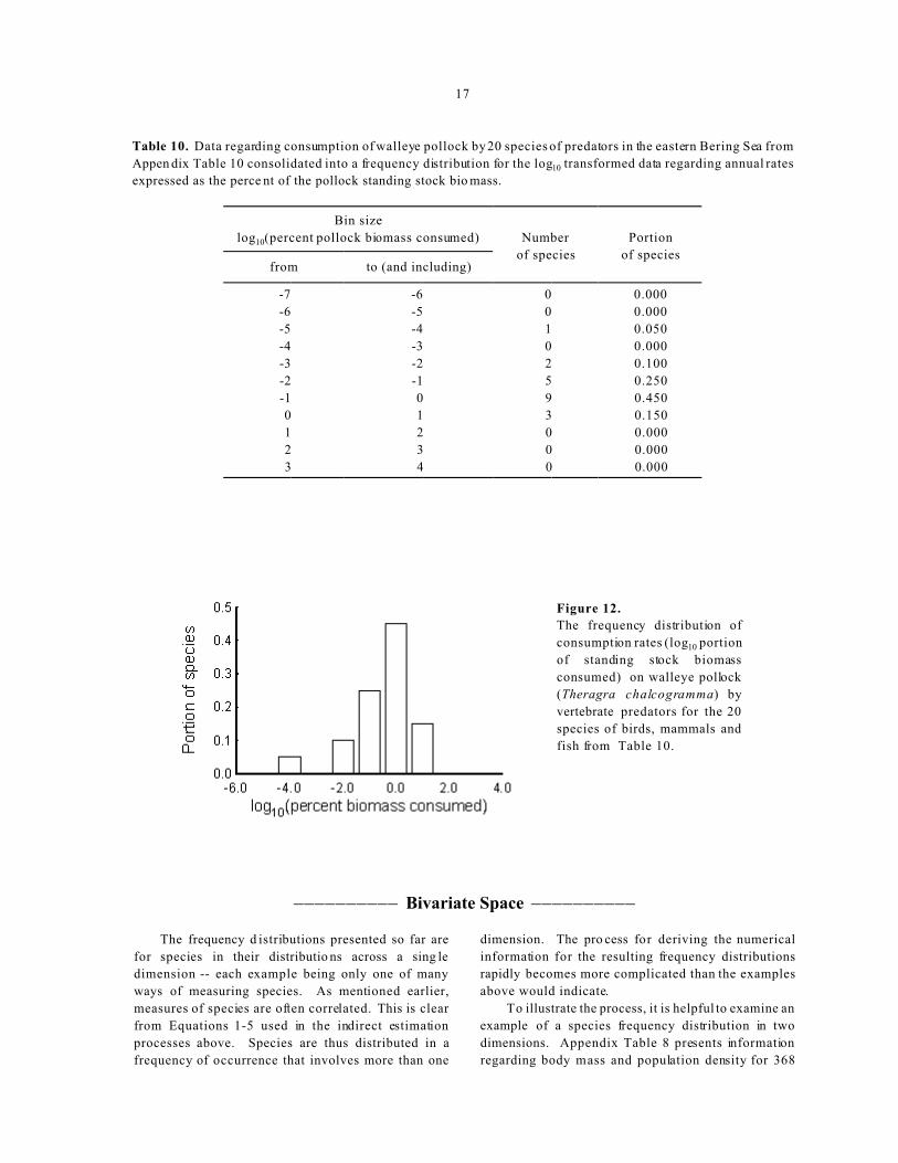
Table 10. Data regarding consumption of walleye pollock by 20 species of predators in the eastern Bering Sea from

Appen dix Table 10 consolidated into a frequency distribution for the log10 transformed data regarding annual rates

expressed as the perce nt of the pollock standing stock bio mass.

Bin size

log10(percent pollock biomass consumed) Number

of species

Portion

of speciesfrom to (and including)

-7 -6 0 0.000

-6 -5 0 0.000

-5 -4 1 0.050

-4 -3 0 0.000

-3 -2 2 0.100

-2 -1 5 0.250

-1 0 9 0.450

0 1 3 0.150

1 2 0 0.000

2 3 0 0.000

3 4 0 0.000

Figure 12.

The frequency distribution of

consumption rates (log10 portion

of standing stock biomass

consumed) on walleye pollock

(Theragra chalcogramma) by

vertebrate predators for the 20

species of birds, mammals and

fish from Table 10.

)))))))))) Bivariate Space ))))))))))

The frequency d istributions presented so far are

for species in their distributio ns across a sing le

dimension -- each example being only one of many

ways of measuring species. As mentioned earlier,

measures of species are often correlated. This is clear

from Equations 1-5 used in the indirect estimation

processes above. Species are thus distributed in a

frequency of occurrence that involves more than one

dimension. The pro cess for deriving the numerical

information for the resulting frequency distributions

rapidly becomes more complicated than the examples

above would indicate.

To illustrate the process, it is helpful to examine an

example of a species frequency distribution in two

dimensions. Appendix Table 8 presents information

regarding body mass and population density for 368

18

species of terrestrial mammalian herbivore s. Table 11

shows the frequency distribution of these species

broken down into categories involving both mass and

density. The process that we have already outlined for

individual dimensions was simply repeated for each

subdivision of the second dimension. For example, all

species with body mass between 2.5 and 3.0 (log scale)

were subdivided into bins of density as if each such

group of species in its respective body-size category

were a single, independent sample. This was repeated

for the remaining data subdivided according to each

respective b ody-size cate gory.

Table 11. A two-dimensional frequency distribution showing the frequency of occurrence of 368 species of

terrestrial mammalian herbivores simultaneously in size (log10 body mass in grams, increasing from left to right) and

density categories (log10 individuals per square kilometer, increasing from bottom to top) based on the data in

Appen dix Table 8. The top panel (a) shows counts of individual species; the lower panel (b) shows the portions of

the sample of 368 species that fall within the size/density bins. Bins without species (zeros) are left blank.

a.

Upper

limit of

density

increments

Count of individual species

Upper limit of body mass increments (log10 grams)

0.5 1.0 1.5 2.0 2.5 3.0 3.5 4.0 4.5 5.0 5.5 6.0 6.5 7.0

5.0

4.5 3 2

4.0 6 11 4 3

3.5 2 12 20 14 1 2

3.0 4 11 22 6 7 4 1

2.5 2 2 10 13 6 7 10 2

2.0 9 4 4 9 13 5

1.5 1 2 3 3 7 14 6 7 2

1.0 1 1 2 4 14 5 4 1 1

0.5 1 4 10 8 1 1

0.0 1 2 5 8 7 2

-0.5 1 3 3 1

-1.0 1

-1.5

b.

Upper

limit of

density

increments

Portion of species

Upper limit of body mass increments (log10 grams)

0.5 1.0 1.5 2.0 2.5 3.0 3.5 4.0 4.5 5.0 5.5 6.0 6.5 7.0

5.0

4.5 0.008 0.005

4.0 0.016 0.030 0.011 0.008

3.5 0.005 0.033 0.054 0.038 0.003 0.005

3.0 0.011 0.030 0.060 0.016 0.019 0.011 0.003

2.5 0.005 0.005 0.027 0.035 0.016 0.019 0.027 0.005

2.0 0.024 0.011 0.011 0.024 0.035 0.014

1.5 0.003 0.005 0.008 0.008 0.019 0.038 0.016 0.019 0.005

1.0 0.003 0.003 0.005 0.011 0.038 0.014 0.011 0.003 0.003

0.5 0.003 0.011 0.027 0.022 0.003 0.003

0.0 0.003 0.005 0.014 0.022 0.019 0.005

-0.5 0.003 0.008 0.008 0.003

-1.0 0.003

-1.5

19

A variety of graphic presentations are possible for

two-dimensional information. One is shown in

Figure 13, which is simply a p lot of the raw d ata in a

scatter plot. The den sity of points and their distribution

is obvious, as is the correlation between mass and

density in the log scale (mentioned above in relation to

estimating density; Peters 1983, Damuth 1987).

Another option for graphic presentation of such

information is shown in Figure 14. Here there are three

panels that combine four columns each from Table 11

(i.e., each panel represen ts a specific range of body size

with body mass for the top panel larger than that of the

bottom).

Figure 13.

Population density of 368

terrestrial mammalian herbivore

species in relation to adult body

mass (Damuth 1987) from

Appendix Table 2 to show the

density of species represented

by density of plotted points.

Figure 14.

The frequency distribution of

population density (log10

numbers per km2) for 368

s p e c i e s o f t e r r e s t r i a l

mammalian herbivores in

three different size categories

from Appendix Tables 8:

Panel A is for species with log

body mass (log10 grams)

between 1 and 2.5; Panel B is

for log body mass between 2.5

to 4.5, and Panel C is for log

body mass between 4.5 to 6.5.

20

A third option is that of a three-dimensional bar

graph (Fig. 15). This graph, as a whole, represents a

two-dimensional frequency d istribution. W ithin this

graph there are essentially one-dimensional frequency

distributions along any cross-section. For example, a

cross-section parallel to the y-axis (the body size

increment he ld constant) would look similar to one of

the graphs of Figure 14.

Any pairwise co mbination o f measures can be used

to construct a species frequency distribution such as

those presented in Figures 13 -15. Anoth er examp le of

this type of information is shown in Figure 16 which

illustrates the relationship between body size and

geographic range (from Brown and Nicoletto 1991).

Figure 15.

A three-dimensional bar graph

s h o w i n g t h e f r e q u e n c y

distribution of popula tion density

(log10 numbers per km2) for 368

species of terrestr ial mammalian

herbivores in 14 different size

categories from Table 11.

Figure 16.

A three-dimensional bar graph

showing the frequenc y distribution

of geographic range size (log10

km2) for terrestrial mammals of

various body masses from Brown

and Nicoletto ( 1991) . Category 1

contains species of less than 16 g

body mass, category 2 is from 16

to 128 g, with a n eight-fold

increase in each higher catego ry,

and category 6 is species larger

than 65,536 g.

21

)))))))))) More Complex Correlations ))))))))))

In progressing from two to three dimensions, we

encounter even more constraints when presenting d ata

in tables and grap hs. To take this step in tabular form,

we could extrapolate from the process outlined above

for cases with two dimensions. To add the third

dimension, we could produce a multi-paged table; each

page would be similar in design to that of Table 11.

Each page of the three-dimensional table would

represent a different bin for one of the three variables.

Each individual three-dimensio nal bin is now like a

cube and is represented by a single element on one of

the pages (as a sub-table of the entire multi-paged

table). Counts of sp ecies would occupy these cubes in

the page/category-specific tables like the top panel of

Table 11. The portions of species found in each bin

would also occur in such tables with information like

that of the bottom panel of Table 11. In m any cases,

the size of such a table would rapidly become

voluminous and impra ctical, but, up to a point, cou ld

be stored on co mputers for analysis.

Graphic ally depicting frequency distributions for

species in three-dimen sional space is impo ssible with

printed histograms or bar graphs. The remaining

option is that of showing the data plotted in three-

dimensional space as demonstrated in Figure 17 (with

hypothetical data showing the interrelationships among

population density, population variation and body

size). Here the density of points in space is

representative of the frequency of species in the cubes

of space defined by the bins for all three me asures of a

species. The three-dimensional visualization p ossible

in the stereogram (bottom section of Figure 17 for the

same data as presented in the larger dots of the top

section) is comparable to similar presentations in two-

dimensional space (e.g., Fig. 13).

Figure 17.

A cluster of hypothetical species

(heavy points in the top panel)

distributed in three-dimensional space

(shown projected in each two-

dimensional combina tion on the wa lls

and floor of the top section, and as a

stereogram in the bottom section)

much as might be expected for

populati on variability, body size, and

population density (the latter two

v a r i a b l e s s h o w n a f t e r l o g10

transformation).

22

All species occur in multidimensional space, of

course, and the task o f defining their freq uency in the

more complex n-dimensional compartments (a cube for

three-dimensional cases) is an extension of the process

begun above in progressing from one dimension, then

to two, and finally to th ree dimen sions. Printed gra phic

presentation becomes impossible beyond three

dimensions without resorting to multiple graphs. With

computer technology, however, data can be analyzed

and through the re petitive video display of mu ltiple

graphs it is po ssible to include other dimension s (e.g.,

time).

)))))))))) Use of Species Frequency Distributions ))))))))))

In our introdu ctory remar ks, we mentio ned an

alternative form of management that makes use of

species frequency d istributions. In this m anageme nt,

the central tendencies of such distributions provide

standards of comp arison and specific mea surable goals

or objectives for management (e.g., control of human

influence on individual species, ecosystems, or the

biosphere). Species frequency distributions provide

guidance for management because they are based on

empirical examples of sustainability represented by

species that have survived the risks associated with

being elements of complex systems (e.g., ecosystems)

as well as through being comp lex systems themselves.

Figures 18, 19, and 20 illustrate where humans are

located on a variety of such frequ ency distributio ns. In

some cases, humans are located in the tails of the

distributions, and in many cases are clear outliers.

Successful managem ent would result in humans (and

hopefully other outlying sp ecies, through their

responses to human action) falling within the normal

range of natural variation, optimally in more central

locations within such distributions (as humans do for

trophic level, Fig. 18A). Maximal sustainability for

humans would be achieved close to the central

tendencies when such c entral tenden cies are: 1) from

collections of species unaffected by abnormal

influence, and 2) representative of species otherwise

similar to humans (e.g., similar body size a s shown in

Figs. 13 and 16). Human interactions and influences

on other systems (e.g., species, ecosystems) are the

only things over which we have much con trol.

Sustainability for our species is of special importance,

but depend s on the cap acity of other syste ms to sustain

us, thus emph asizing the nee d to chang e in order to

achieve system ic sustainability.

Now we can see that the bias of estimation

procedures would have to be extreme to be misleading

regarding the magnitude, but especially the direction,

of change required for effective management. Even so,

measures of the extent of change required of humans

through effective mana gement ma y be substantiv ely

affected by bias. Such bias can come both from

procedural effects (e.g., error in estimation), as well as

the effects of influence by outlying spe cies, especia lly

humans, on existing distributions.

Management based on empirical examples

addresses a number of problems and issues that have

frustrated past attempts to achieve maximal

sustainability. It is simultaneou sly applicab le with

regard to ecosystems (Fig. 18B), taxonomic groups of

species (Fig. 11B), single species resources (Fig. 18C),

and the biosphere (Fig. 18F; also Fowler 1999, Fowler

et al. 1999, Fowler unpub. manuscript) as shown in

Figure 20. It applies in a variety of ways (Figs. 18, 19

and 20). Control, in this form of manage ment, involves

changes in human activities where control is an option

(e.g., promo ting or limiting commercial fishing

operations rather than controlling fish populations or

their ecosystems; Campbell 1974, Bateson 1979, Allen

and Starr 1982, Salthe 1985, O'Neill et al. 1986,

Wilber 1995, Holling and M effe 1996 , Mange l et al.

1996). Such change and action would be an

application of a core p rinciple of manage ment:

maintaining elements of biological organizatio n within

their normal ranges of natural variation (Christensen et

al. 1996, Mangel et al. 1996) as direct recognition of

the limits to variation (Pickett et al. 1992).

Species frequency distributions are increasingly

recognized as phenom ena of impo rtance in ecological

studies, especially in what has been calle d

"macroecology" (the study of large-scale ecological

patterns, exemplified and defined in Brown 1995; see

also Rosenzw eig 1995 ). As such, the management that

we are describing brings the science of macroecology

into practical application.

Among the forces contributing to the formation of

species frequency distributions are the dynamics of

selective extinction and speciation (Slatkin 1981,

Arnold and Fristrup 1982, Fowler and MacMahon

1982, Levinton 1988, Cristoffer 1990). Extinction is

one of the forces that contributes to preventing the

accumulation of certain types of species (e.g., those in

and beyond the tails of species frequency distributions).

Management based on this approach thus accounts for

the risk of extinction along with the other factors that

contribute to the limits of variation and the positions of

individual species wit hin specie s frequency

distributions.

23

Figure 18.

Frequency distributions among species showing the change needed by humans as management to achieve a position

near central tendencies (e.g., means of the distributions): A) trophic level based on species from 95 insect-

dominated food web s (from Sch oenly et al. 19 91, an examp le of little if any change needed by humans); B) a

frequency distribution representing consumption of biomass from the Georges Bank ecosystem by 24 species of

marine mammals, sea birds and h umans (from Backus a nd Bou rne 198 6); C) con sumption ra te of walleye pollock

(Theragra chalcogramma) by vertebra te predato rs (Fig. 12; hu man cons umption is ab out 60-fold the mean

consumption rate); D) range size (Fig. 6) showing humans at 70% of the Earth's non-Antarctic terrestrial surface

(about 71.4 million km2, although 95 % might b e more rea listic, Pimentel et al. 1992); E) density dependence for

64 species of invertebrates, fish, birds and mammals in five statistical categories (from A: positive and significant

to E: negative and significant at the 0.05 probability level; Tanner 1966, Pimm 1982); F) Total biomass ingested

(i.e., not including biomass used for combustion, construction or other purposes) for humans and the 63 species of

mamma ls from Figure 5 based on relationships form Peters (1983);G) energy consumption per unit area based on

the 386 species of mammalian primary consumers of Damuth (1987) and size-specific energetic estimates based on

relationships from Peters (1983); H) carbon dioxide production (Fig. 9) showing humans at 25 billion tons annually

(Ehrlich and Ehrlich 1996).

24

Figure 19.

Frequency distributions among species showing the change needed by humans as management to achieve a position

near central tendencies (e.g., means of the distributions): A) Human consumption (harvest) of finfish in the Bering

Sea compared to that of various species of marine mammals from Figure 11; B) The total populations of marine

mamma ls from the co llection dep icted in Figure 5 in comparison to the total population of humans; C) The

consumption of mackere l, herring, sand e el, and hake by consum ers in the northw est Atlantic com pared to

consumption (harvest) of the same species by humans (corresponding to the consumption of these species by

dogfish, Overholtz et al. 1991); D) The total populations of terrestrial mammals fro m the collec tion depicte d in

Figure 5 in comparison to the total population of humans; E) The consumption of lantern fish, lightfish, anchovy

and hake by consumers (33 species of marine birds) in the ecosystem off the southwest coast of Africa compared

to consumption (harvest) of the same species by humans (from Crawford et al. 1991); F) The combination of B and

D above (a lso the distributio n of Fig. 5 exp anded) to show the human population (5.7 billion) several orders of

magnitude larger than the mean; G) The consumption of anchovy by consumers (33 species of marine birds) in the

ecosystem(s) off the southwest coast of Africa compared to consumption (harvest) by humans (from Crawford et al.

1991); H) The consumption of biomass by consumers (33 species of marine birds) in the ecosystem(s) off the

southwest coast of Africa compared to consumption (harvest) by humans (from Crawford et al. 1991).

25

Figure 20.

The frequency distribution of consumption rates

for marine mammals showing consumption rates

at a variety of levels of biological o rganization in

comparison to the rate at which humans harvest

biomass. The top panel show s the natural

variation in consumption of pollock as observed

for 6 specie s of marine mammals in the Bering

Sea in comparison to recent takes of pollock by

commercial fisheries (com pare to Fig. 19C) . The

second panel shows consumption of finfish in the

Bering Sea by 20 species of m arine mam mals

compared to fisheries takes (see Fig. 11). Total

biomass consumption is shown for 20 species of

marine mamma ls in the Bering Sea in the third

panel, again compared to the commercial take

which is predominantly pollock (see Fig. 11).

Total biomass consumption for the entire marine

environment is shown in the fo urth panel for 55

species of marine m ammals, he re comp ared to

the take of about 110 million metric tons

estimated as the harvest o f biomass for human

use in the late 1990s (Committee on Ecosystem

Management for Sustainable Marine Fisheries

1999). World-wide consumption of biomass by

humans is compar ed to that of the same 55

species of marine m ammals in the bottom panel.

The last two panels are based on population and

body size data from the marine mammal series by

Ridgway and Harrison (1981-99) and equations

representing ingestion rates as a function of body

size in Peters (1983).

Keeping ecosystems th emselves with in their

normal ranges of natural variation has been suggested

as a goal for management (Rapport et al. 1981, Rapport

et al. 1985), but action to control ecosystems is not

considered an option (Campbell 1974, Bateson 1979,

Allen and Starr 1982, Salthe 1985, O'Neill et al. 1986,

Wilber 1995, Holling and Meffe 1996, M angel et al.

1996). The remaining alternative is that of

management defined to include human species-level

change, constraint, and action. Such changes,

constraints an d action are within our species purview.

They are changes where control is an option (Holling

and Meffe 1996, Fowler unpub. manuscrip t), difficult

as any such changes may be. Applied at the level of

ecosystems and the biosphere, our influence on

ecosystems and the biosphere would be controlled.

Human influence would b e constraine d to fall within

the normal ranges of natural variation exhibited among

species. Thus, it is important to know how to construct

species frequency distributions to provide the needed

information concerning such variation and its limits.

The data chosen for any particular distribution

must be specific to the management question being

addressed. Thus, to address the question of what is the

most sustainable level of biomass consumption from a

particular ecosystem, data such as shown in Figure 11A

and Figures 18, 19 and 20 would be used. If the

question is related to most sustainable harvest rate from

the finfish of the Bering Sea, data like that of Figure

11B (see also Fig. 19A and second panel of Fig. 20)

26

would be used. Fin ding the most sustainable tro phic

level would be guided by data such as those show n in

Figure 8. The process is more complicated than can be

readily described here, involving am ong other things,

the need to take into account the factors contributing to

the variation observed in species frequency

distributions (Fowler 1999, Fowler et al. 1999, Fowler

unpub. manuscript), and data for species otherwise

similar to humans.

Although fairly straight-forward in concept, such

management would face serious challenges in

implementation. For example, reducing commercial

takes of fish by one or two orde rs of magnitude (Figs.

18B, 18C, 19A, 19C, 19E, 19G, 19H and 20)

represents major change. The management

implications obviated by the information such as that

shown in Figu res 18, 19 and 20 a re not trivial.

Adding to such challenges are complicating factors

such as the need to ensure that the sample of species

chosen for guidance are sp ecies that are simila r to

humans in regard to features other than those for which

guidance is sought. Th is is because certain measures of

species are related to others. Such relationships are

exemplif ied by population density (Fig. 15) and

distribution (Fig. 16) in relationship to body mass. But

body size is not the only factor for such consideration.

Because of the complexity of nature, other factors such

as similarity of trophic level, for example, must also be

considered when selecting species to construct

informative frequency d istributions to guide

management. Such issues, however, are beyond the

scope of this paper. They emphasize the importance of

adequa te data and clear graphic presentation of species

frequency distributions. Here we have focused on the

process of the analysis and display of such information

to usefully depict the distributions represented.

It should be noted that the p receding discuss ion

also applies to the assessment of any aberrant species.

That is, species frequency distributions can be applied

to the measure of species other than humans. Although

complete control of o ther species a nd their

relationships with other bio logical systems is n ot an

option, species freq uency distr ibutions can still serve

among the importa nt tools at our d isposal. It is

important to successful m anageme nt to identify

problems that emerge from the collective influence of

the variety of ways humans are found outside the

normal ranges of natu ral variation. T his is not only

important in assessing individual species (e.g., the

status of endangered species) but also is important at

the ecosystem le vel in addre ssing the positio n and

shapes of such distributions that characterize such

systems.

)))))))))) Summary ))))))))))

Species frequency distributions can be constructed

using any of a very large variety of measures that

describe the natural variation of species. There are

several critical steps. First, measurements are collected

for a sample of species. Second, the measurements are

ordered and subdivided into groups co rrespond ing to

uniform categories, increments, or bins, often after

transformation of the data (e.g., frequently a log10

transform). Third, the number of species in each

category are counted and the count is conv erted to

either a portion, or a percent, of the total sample.

Finally, these portio ns (or perc ents) are plo tted in

histograms to graphica lly present the distribution for

visual perception of the underlying proba bility

distribution to see variability an d its limits. The ba sic

steps are laid out in many elementary statistical texts as

applied to any form of measurement, here exemplified

by measures of species shown in a variety of tables and

graphs. After the data are collected, the remaining

steps can be ach ieved with relative ease in many of the

software application s available for data ana lysis today.

Measu rements of species can include a wide

variety of variables. Examples are: population size,

population variation, mean adult body size, total

metabolic rates, geographic range size, portion of a

prey species' biom ass consum ed, chrom osome c ount,

carbon dioxide produced, energy consumed, or

intrinsic rates of increase. Others would include

consumption rates for nitrogen (or any other element),

mobility, mortality rates, total biomass, and

suppressing effects on resource species. It is not clear

that there is a limit to such a list. As has been

demonstrated in a variety of scien tific publications,

there are relationships between and among many such

measures, some of which form consistent higher-level

patterns (e.g., Charnov 1993). Frequency distributions

in two-dimensional space can show such relationships

and the distribution of species within them. Three-

dimensional relationships can be depic ted in

stereograms, but not in ordinary frequency

distributions. Graphic demonstration of frequency

distributions in more than three dimensions is not

27

simple. However, it is possible to take advantage of

sophisticated graphic software and modern computers

to make useful presentations of data.

The utility of species frequency distributions stems

from their demonstration of the limits and central

tendencies in the variation among species. We need

such information to find the prop er place for aberrant

species (including hum ans) as sustaina ble comp onents

of ecosystems or the biosphere by falling within the

normal range of natural variation. Data chosen for

guidance must always be specific to the management

question being addressed.

)))))))))) Acknowledgments ))))))))))

We thank Martin D orn, Gary D uker, Lisa H iruki,

Sue Hills, James Lee, Bernard Megrey, and Rod

Towell for very helpful rev iews and co mments. We are

also thankful to each of the individuals and teams who

spent many hour s, often large po rtions of their

professional careers, in the production of sets of data

that we used in d emonstratin g the construction of

species freq uency distribu tions. These people are too

numerous to name but are cited with our tables and

figures (our citations often open a trail of references to

establish their identity). It takes much time and effort

to produce data of the kind that can be used in

producing species frequency distributions and we want

to acknowledge the people involved.

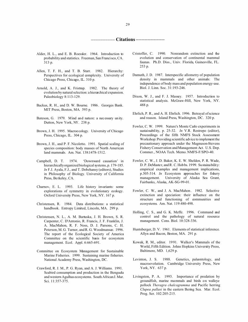
29

)))))))))) Citations ))))))))))

Alder, H. L., and E. B. Roessler. 1964. Introduction toprobability and statistics. Freeman, San Francisco, CA.313 p.

Allen, T. F. H., and T. B. Starr. 1982. Hierarchy:Perspectives for ecological complexity. University ofChicago Press, Chicago, IL. 310 p.

Arnold, A. J., and K. Fristrup. 1982. The theory ofevolution by natural selection: a hierarchical expansion.Paleobiology 8:113-129.

Backus, R. H., and D. W. Bourne. 1986. Georges Bank.MIT Press, Boston, MA. 593 p.

Bateson, G. 1979. Mind and nature: a necessary un ity.Dutton, New York, NY. 238 p.

Brown, J. H. 1995. Macroecology. University of ChicagoPress, Chicago, IL. 304 p.

Brown, J. H., and P. F. Nicoletto. 1991. Spatial scaling ofspecies composition: body masses of North Americanland mammals. Am. Nat. 138:1478-1512.

Campbell, D. T. 1974. ‘Downward causation’ inhierarchically organized biological systems, p. 179-185.In F.J. Ayala, F.J., and T. Dobzhansy (editors), Studiesin Philosophy of Biology. University of CaliforniaPress, Berkeley, CA.

Charnov, E. L. 1993. Life history invariants: someexplorations of symmetry in evolutionary ecology.Oxford University Press, New York, NY. 167 p.

Christensen, R. 1984. Data distributions: a statisticalhandbook. Entropy Limited, Lincoln, MA. 299 p.

Christensen, N. L., A. M. Bartuska, J. H. Brown, S. R.Carpenter, C. D'Antonio, R. Francis, J. F. Franklin, J.A. MacMahon, R. F. Noss, D. J. Parsons, C. H.Peterson, M. G. Turner, and R. G. Woodmansee. 1996.The report of the Ecological Society of AmericaCommittee on the scientific basis for ecosystemmanagement. Ecol. Appl. 6:665-691.

Committee on Ecosystem Management for SustainableMarine Fisheries. 1999. Sustaining marine fisheries.National Academy Press, Washington, DC.

Crawford, R. J. M., P. G. Ryan, and A. J. Williams. 1991. Seabird consumption and production in the Benguelaand western Agulhas ecosystems. South African J. Mar.Sci. 11:357-375.

Cristoffer, C. 1990. Nonrandom extinction and theevolution and conservation of continental mammalfaunas. Ph.D. Diss., Univ. Florida, Gainesville, FL.253 p.

Damuth, J. D. 1987. Interspecific allometry of populationdensity in mammals and other animals: Theindependence of body mass and population energy-use.Biol. J. Linn. Soc. 31:193-246.

Dixon, W. J., and F. J. Massey. 1957. Introduction tostatistical analysis. McGraw-Hill, New York, NY.488 p.

Ehrlich, P. R., and A. H. Ehrlich. 1996. Betrayal of scienceand reason. Island Press, Washington, DC. 320 p.

Fowler, C. W. 1999. Nature's Monte Carlo experiments insustainabil ity, p. 25-32. In V.R. Restrepo (editor),Proceedings of the fifth NMFS Stock AssessmentWorkshop: Providing scientific advice to implement theprecautionary approach under the Magnuson-StevensFishery Conservation and Management Act. U.S. Dep.Commer., NOAA Tech. Memo. NMFS-F/SPO-40.

Fowler, C. W., J. D. Baker, K. E. W. Shelden, P. R. Wade,D. P. DeMaster, and R. C. Hobbs. 1999. Sustainability:empirical examples and management implications,p.305-314. In Ecosystem approaches for fisherymanagement. University of Alaska Sea Grant,Fairbanks, Alaska, AK-SG-99-01.

Fowler, C. W., and J. A. MacMahon . 1982. Selectiveextinction and speciation: their influence on thestructure and functioning of communities andecosystems. Am. Nat. 119:480-498.

Holling, C. S., and G. K. Meffe. 1996. Command andcontrol and the pathology of natural resourcemanagement. Cons. Biol. 10:328-336.

Huntsberger, D. V. 1961. Elements of statistical inference.Allyn and Bacon, Boston, MA. 291 p.

Kowak, R. M., editor. 1991. Walker's Mammals of theWorld, Fifth Edition. Johns Hopkins University Press,Baltimore, MD. 1,629 p.

Levinton, J. S. 1988. Genetics, paleontology, andmacroevolution. Cambridge University Press, NewYork, NY. 637 p.

Livingston, P. A. 1993. Importance of predation bygroundfish, marine mammals and birds on walleyepollock Theragra chalcogramma and Pacific herringClupea pallasi in the eastern Bering Sea. Mar. Ecol.Prog. Ser. 102:205-215.

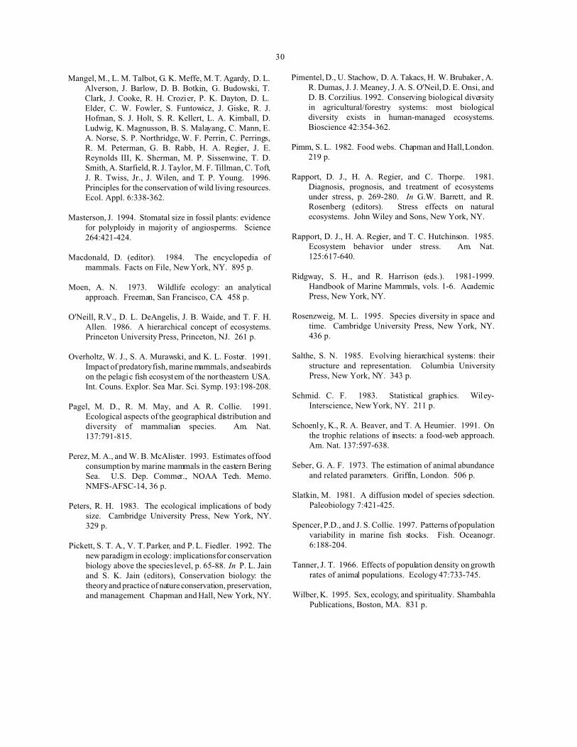
30

Mangel, M., L. M. Talbot, G. K. Meffe, M. T. Agardy, D. L.Alverson, J. Barlow, D. B. Botkin, G. Budowski, T.Clark, J. Cooke, R. H. Crozier, P. K. Dayton, D. L.Elder, C. W. Fowler, S. Funtowicz, J. Giske, R. J.Hofman, S. J. Holt, S. R. Kellert, L. A. Kimball, D.Ludwig, K. Magnusson, B. S. Malayang, C. Mann, E.A. Norse, S. P. Northridge, W. F. Perrin, C. Perrings,R. M. Peterman, G. B. Rabb, H. A. Regier, J. E.Reynolds III, K. Sherman, M. P. Sissenwine, T. D.Smith, A. Starfield, R. J. Taylor, M. F. Tillman, C. Toft,J. R. Twiss, Jr., J. Wilen, and T. P. Young. 1996.Principles for the conservation of wild living resources.Ecol. Appl. 6:338-362.

Masterson, J. 1994. Stomatal size in fossil plants: evidencefor polyploidy in majority of angiosperms. Science264:421-424.

Macdonald, D. (editor). 1984. The encyclopedia ofmammals. Facts on File, New York, NY. 895 p.

Moen, A. N. 1973. Wildlife ecology: an analyticalapproach. Freeman, San Francisco, CA. 458 p.

O'Neill, R.V., D. L. DeAngelis, J. B. Waide, and T. F. H.Allen. 1986. A hierarchical concept of ecosystems.Princeton University Press, Princeton, NJ. 261 p.

Overholtz, W. J., S. A. Murawski, and K. L. Foster. 1991.Impact of predatory fish, marine mammals, and seabirdson the pelagic fish ecosystem of the northeastern USA.Int. Couns. Explor. Sea Mar. Sci. Symp. 193:198-208.

Pagel, M. D., R. M. May, and A. R. Collie. 1991.Ecological aspects of the geographical distribution anddiversity of mammalian species. Am. Nat.137:791-815.

Perez, M. A., and W. B. McAlister. 1993. Estimates of foodconsumption by marine mammals in the eastern BeringSea. U.S. Dep. Commer., NOAA Tech. Memo.NMFS-AFSC-14, 36 p.

Peters, R. H. 1983. The ecological implications of bodysize. Cambridge University Press, New York, NY.329 p.

Pickett, S. T. A., V. T. Parker, and P. L. Fiedler. 1992. Thenew paradigm in ecology: implications for conservationbiology above the species level, p. 65-88. In P. L. Jainand S. K. Jain (editors), Conservation biology: thetheory and practice of nature conservation, preservation,and management. Chapman and Hall, New York, NY.

Pimentel, D., U. Stachow, D. A. Takacs, H. W. Brubaker , A.R. Dumas, J. J. Meaney, J. A. S. O'Neil, D. E. Onsi, andD. B. Corzilius. 1992. Conserving biological diversityin agricultural/forestry systems: most biologicaldiversity exists in human-managed ecosystems.Bioscience 42:354-362.

Pimm, S. L. 1982. Food webs. Chapman and Hall, London.219 p.

Rapport, D. J., H. A. Regier, and C. Thorpe. 1981.Diagnosis, prognosis, and t reatment of ecosystemsunder stress, p. 269-280. In G.W. Barrett, and R.Rosenberg (editors). Stress effects on naturalecosystems. John Wiley and Sons, New York, NY.

Rapport, D. J., H. A. Regier, and T. C. Hutchinson. 1985.Ecosystem behavior under stress. Am. Nat.125:617-640.

Ridgway, S. H., and R. Harrison (eds.). 1981-1999.Handbook of Marine Mammals, vols. 1-6. AcademicPress, New York, NY.

Rosenzweig, M. L. 1995. Species diversity in space andtime. Cambridge University Press, New York, NY.436 p.

Salthe, S. N. 1985. Evolving hierarchical systems: theirstructure and representation. Columbia UniversityPress, New York, NY. 343 p.

Schmid. C. F. 1983. Statistical graphics. Wiley-Interscience, New York, NY. 211 p.

Schoenly, K., R. A. Beaver, and T. A. Heumier. 1991. Onthe trophic relations of insects: a food-web approach.Am. Nat. 137:597-638.

Seber, G. A. F. 1973. The estimation of animal abundanceand related parameters. Griffin, London. 506 p.

Slatkin, M. 1981. A diffusion model of species selection.Paleobiology 7:421-425.

Spencer, P.D., and J. S. Collie. 1997. Patterns of populationvariability in marine fish stocks. Fish. Oceanogr.6:188-204.

Tanner, J. T. 1966. Effects of population density on growthrates of animal populations. Ecology 47:733-745.

Wilber, K. 1995. Sex, ecology, and spirituality. ShambahlaPublications, Boston, MA. 831 p.

31

))))))Appendix ))))))

Appendix Tables 1 through 11

33

Appen dix Table 1. List of 103 species of marine mammals with measures o f their adult body mass. Columns A

and G are species number, B indicates the primary source of information (see footnotes), C indicates the type of data

(see footnotes), D is the species name, E and H are the body mass in kilograms, F and I are the log10 of body mass.

Columns A, B, C, D, E, and F are in ord er by scientific nam e and colu mns G, H , and I are in order by bod y mass.

A B C D E F G H I

1 1 2 Arctocep halus au stralis 104.0 2.017 27 27.2 1.434

2 1 1 Arctocepha lus forsteri 103.8 2.016 70 37.5 1.574

3 1 2 Arctocep halus ga lapago ensis 45.5 1.658 21 40.0 1.602

4 1 2 Arctocep halus ga zella 83.5 1.922 22 40.0 1.602

5 1 2 Arctocep halus ph ilippii 90.0 1.954 88 42.5 1.628

6 1 2 Arctocephalus pusillus 411.0 2.614 20 45.0 1.653

7 1 2 Arctocep halus trop icalis 110.0 2.041 3 45.5 1.658

8 1 3 Balaen a glacialis 53,000 .0 4.724 19 50.0 1.699

9 1 3 Balaena mysticetus 70,000 .0 4.845 77 55.0 1.740

10 1 5 Balaen optera a cutorostra ta 10,000 .0 4.000 89 55.0 1.740

11 1 5 Balaen optera b orealis 30,000 .0 4.477 87 59.5 1.775

12 1 5 Balaenoptera edeni 26,000 .0 4.415 49 60.0 1.778

13 1 5 Balaenoptera musculus 150,00 0.0 5.176 48 70.0 1.845

14 1 5 Balaenoptera physalus 80,000 .0 4.903 80 71.3 1.853

15 1 3 Berardius arnuxi 10,200 .0 4.009 82 72.0 1.857

16 1 2 Berard ius bairdii 14,250 .0 4.154 86 72.0 1.857

17 1 1 Callorhinus ursinus 135.8 2.133 95 75.0 1.875

18 1 3 Capere a marg inata 3,250.0 3.512 25 80.0 1.903

19 1 5 Cephalorhynchus commersoni 50.0 1.699 4 83.5 1.922

20 1 5 Cepha lorhync hus eutro pia 45.0 1.653 81 85.0 1.929

21 1 5 Cepha lorhync hus hea visidii 40.0 1.602 92 85.0 1.929

22 1 5 Cephalorh ynchus hec tori 40.0 1.602 5 90.0 1.954

23 1 2 Cystoph ora cristata 360.0 2.556 40 90.0 1.954

24 1 3 Delphinapterus leucas 1,000.0 3.000 45 90.0 1.954

25 1 2 Delphin us delph is 80.0 1.903 78 95.0 1.978

26 1 3 Dugong dugon 565.0 2.752 44 100.0 2.000

27 2 1 Enhyd ra lutris 27.2 1.434 73 100.0 2.000

28 1 5 Erignathus barbatus 190.0 2.279 83 100.0 2.000

29 1 2 Eumetopias jubatus 636.5 2.804 93 100.0 2.000

30 1 2 Feresa a ttenuata 160.0 2.204 94 100.0 2.000

31 1 5 Globicephala macrorhynchus 1,900.0 3.279 2 103.8 2.016

32 1 5 Globicephala melaena 2,650.0 3.423 1 104.0 2.017

33 1 2 Grampus griseus 375.0 2.574 7 110.0 2.041

34 1 1 Halichoerus grypus 227.5 2.357 96 110.0 2.041

35 1 2 Hydrurga leptonyx 347.5 2.541 43 115.0 2.061

36 1 4 Hyperoodon ampullatus 10,000 .0 4.000 46 115.0 2.061

37 1 2 Hyperoodon planifrons 7,050.0 3.848 79 130.0 2.114

38 1 5 Kogia breviceps 500.0 2.699 97 130.0 2.114

39 1 5 Kogia simus 350.0 2.544 17 135.8 2.133

40 1 5 Lagenodelphis hosei 90.0 1.954 85 147.5 2.169

41 1 2 Lagenorhynchus acutus 190.0 2.279 30 160.0 2.204

42 1 5 Lagen orhync hus albiro stris 190.0 2.279 76 160.0 2.204

43 1 5 Lagen orhync hus aus tralis 115.0 2.061 101 175.0 2.243

44 1 5 Lagenorhynchus cruciger 100.0 2.000 72 179.5 2.254

45 1 5 Lagenorhynchus obliquidens 90.0 1.954 102 183.0 2.262

34

Appendix Table 1. (Continued)

A B C D E F G H I

46 1 5 Lagenorhynchus obscurus 115.0 2.061 69 188.6 2.275

47 1 2 Lepton ychotes w eddelli 420.0 2.623 28 190.0 2.279

48 1 5 Lissodelp his borea lis 70.0 1.845 41 190.0 2.279

49 1 5 Lissodelp his peron ii 60.0 1.778 42 190.0 2.279

50 1 5 Lobodon carcinophagus 220.0 2.342 67 200.0 2.301

51 1 5 Megaptera novaeangliae 65,000 .0 4.813 66 210.0 2.322

52 1 5 Mesoplodon bidens 3,400.0 3.531 50 220.0 2.342

53 1 5 Mesoplodon bowdoini 2,600.0 3.415 34 227.5 2.357

54 1 5 Mesoplod on carlhub bsi 3,400.0 3.531 75 232.0 2.365

55 1 5 Mesop lodon d ensirostris 3,600.0 3.556 65 280.0 2.447

56 1 5 Mesoplodon europaeus 5,600.0 3.748 84 315.0 2.498

57 1 5 Mesoplodon ginkgodens 3,600.0 3.556 35 347.5 2.541

58 1 5 Mesoplodon grayi 4,800.0 3.681 39 350.0 2.544

59 1 5 Mesoplod on hectori 2,000.0 3.301 23 360.0 2.556

60 1 5 Mesop lodon la yardii 3,400.0 3.531 33 375.0 2.574

61 1 5 Mesoplodon mirus 3,200.0 3.505 6 411.0 2.614

62 1 5 Mesoplod on stejnegeri 4,800.0 3.681 47 420.0 2.623

63 1 2 Miroun ga ang ustirostris 1,600.0 3.204 99 425.0 2.628

64 1 2 Mirounga leonina 1,540.0 3.188 38 500.0 2.699

65 1 2 Monachus monachus 280.0 2.447 26 565.0 2.752

66 1 2 Monachus schauinslandi 210.0 2.322 29 636.5 2.804

67 1 5 Mona chus trop icalis 200.0 2.301 71 850.0 2.929

68 1 3 Monodon monoceros 1,200.0 3.079 24 1,000.0 3.000

69 1,2 2 Neophoca cinerea 188.6 2.275 68 1,200.0 3.079

70 1 3 Neophocoena phoconoides 37.5 1.574 64 1,540.0 3.188

71 1 1 Odobenus rosmarus 850.0 2.929 63 1,600.0 3.204

72 2 2 Omm atophoca rossi 179.5 2.254 91 1,600.0 3.204

73 1 5 Orcaella brevirostris 100.0 2.000 100 1,600.0 3.204

74 1 1 Orcinus orca 3,500.0 3.544 31 1,900.0 3.279

75 1 1 Otaria flavescens 232.0 2.365 59 2,000.0 3.301

76 1 5 Pepono cephala electra 160.0 2.204 53 2,600.0 3.415

77 1 5 Phoca caspica 55.0 1.740 32 2,650.0 3.423

78 1 5 Phoca fasciata 95.0 1.978 61 3,200.0 3.505

79 1 5 Phoca groenlandica 130.0 2.114 18 3,250.0 3.512

80 1 1 Phoca hispida 71.3 1.853 52 3,400.0 3.531

81 1 2 Phoca larga 85.0 1.929 54 3,400.0 3.531

82 1 5 Phoca siberica 72.0 1.857 60 3,400.0 3.531

83 1 1 Phoca vitulina 100.0 2.000 74 3,500.0 3.544

84 1 2 Phocarcto s hookeri 315.0 2.498 55 3,600.0 3.556

85 1 3 Phoco ena da lli 147.5 2.169 57 3,600.0 3.556

86 1 3 Phocoena dioptrica 72.0 1.857 58 4,800.0 3.681

87 1 3 Phocoena phocoena 59.5 1.775 62 4,800.0 3.681

88 1 3 Phocoena sinus 42.5 1.628 56 5,600.0 3.748

89 1 3 Phoco ena spin ipinnis 55.0 1.740 98 5,600.0 3.748

90 1 1 Physeter macrocephalus 37,500 .0 4.574 103 5,600.0 3.748

91 1 2 Pseudorca crassidens 1,600.0 3.204 37 7,050.0 3.848

92 1 5 Sousa c hinensis 85.0 1.929 10 10,000 .0 4.000

93 1 5 Stenella a ttenuata 100.0 2.000 36 10,000 .0 4.000

94 1 5 Stenella coeruleoalba 100.0 2.000 15 10,200 .0 4.009

35

Appendix Table 1. (Continued)

A B C D E F G H I

95 1 5 Stenella lo ngirostris 75.0 1.875 16 14,250 .0 4.154

96 1 5 Stenella plagiodon 110.0 2.041 12 26,000 .0 4.415

97 1 2 Steno b redane nsis 130.0 2.114 11 30,000 .0 4.477

98 1 5 Tasmacetus spepherdi 5,600.0 3.748 90 37,500 .0 4.574

99 1 3 Trichech us inung uis 425.0 2.628 8 53,000 .0 4.724

100 1 5 Trichechus manatus 1,600.0 3.204 51 65,000 .0 4.813

101 1 3 Tursiops truncatus 175.0 2.243 9 70,000 .0 4.845

102 1 2 Zalophus californianus 183.0 2.262 14 80,000 .0 4.903

103 1 5 Ziphius c avirostris 5,600.0 3.748 13 150,00 0.0 5.176

Source (column B):

1: Macdonald (1984)

2: Ridgway and Harrison (1981-99)

Data type (column C):

1: Mean of the midpoints of ranges reported for both sexes

2: Mean of weights reported for each sex

3: Midpo int of range of weights reported for spe cies (both sexes)

4: Weig ht reported for males on ly

5: Single weight reported for species

36

Appen dix Table 2. List of 368 species of terrestrial mammalian primary consumers arrayed in order by their mean

adult body mass measured in kilograms and in log10(kg). The species number is the sequence number of the species

as found with its specific name in Damuth (1987).

Species

number

Mass Species

number

Mass Species

number

Mass

(kg) log10(kg) (kg) log10(kg) (kg) log10(kg)

209 0.005 -2.301 224 0.035 -1.456 231 0.065 -1.187

258 0.006 -2.194 248 0.036 -1.444 238 0.065 -1.187

185 0.007 -2.155 179 0.036 -1.444 219 0.065 -1.187

287 0.007 -2.131 305 0.038 -1.420 272 0.065 -1.187

289 0.008 -2.125 218 0.039 -1.415 202 0.069 -1.163

211 0.008 -2.086 226 0.039 -1.409 230 0.069 -1.161

259 0.009 -2.071 301 0.039 -1.409 229 0.069 -1.161

257 0.009 -2.066 240 0.039 -1.409 308 0.070 -1.155

260 0.012 -1.928 276 0.040 -1.398 181 0.070 -1.155

210 0.014 -1.870 190 0.040 -1.398 250 0.071 -1.149

291 0.015 -1.824 191 0.040 -1.398 336 0.071 -1.149

298 0.015 -1.824 192 0.040 -1.398 184 0.071 -1.149

319 0.016 -1.796 282 0.040 -1.398 217 0.072 -1.143

288 0.017 -1.770 280 0.040 -1.398 309 0.072 -1.143

263 0.018 -1.750 274 0.042 -1.377 278 0.077 -1.116

349 0.018 -1.745 293 0.042 -1.377 236 0.081 -1.092

290 0.020 -1.699 174 0.042 -1.377 317 0.085 -1.071

297 0.020 -1.699 345 0.042 -1.377 271 0.086 -1.066

178 0.020 -1.699 253 0.043 -1.367 206 0.088 -1.056

296 0.021 -1.678 239 0.044 -1.357 347 0.093 -1.032

318 0.021 -1.678 302 0.044 -1.357 227 0.097 -1.013

269 0.021 -1.678 320 0.044 -1.357 340 0.097 -1.013

172 0.022 -1.658 234 0.045 -1.352 337 0.100 -1.000

186 0.023 -1.648 322 0.045 -1.347 342 0.101 -0.996

197 0.023 -1.638 251 0.047 -1.328 182 0.103 -0.987

294 0.023 -1.638 273 0.049 -1.310 333 0.107 -0.971

299 0.024 -1.620 255 0.049 -1.310 215 0.108 -0.967

279 0.024 -1.618 256 0.049 -1.310 261 0.108 -0.967

228 0.026 -1.585 304 0.050 -1.301 286 0.112 -0.951

249 0.027 -1.569 283 0.050 -1.301 314 0.112 -0.951

196 0.027 -1.569 329 0.050 -1.301 321 0.115 -0.939

338 0.027 -1.569 343 0.051 -1.292 246 0.116 -0.936

292 0.028 -1.553 300 0.052 -1.284 327 0.120 -0.921

199 0.028 -1.553 220 0.053 -1.276 285 0.121 -0.917

350 0.029 -1.538 303 0.053 -1.276 313 0.122 -0.914

176 0.029 -1.536 316 0.054 -1.268 311 0.125 -0.903

235 0.030 -1.523 237 0.054 -1.268 177 0.127 -0.896

277 0.030 -1.523 212 0.055 -1.260 328 0.129 -0.889

201 0.031 -1.516 213 0.056 -1.252 267 0.130 -0.886

198 0.031 -1.509 351 0.056 -1.252 284 0.136 -0.866

180 0.033 -1.481 281 0.059 -1.229 183 0.143 -0.845

348 0.034 -1.469 214 0.060 -1.222 216 0.145 -0.839

262 0.034 -1.469 344 0.062 -1.208 221 0.145 -0.839

295 0.035 -1.456 310 0.062 -1.208 173 0.146 -0.836

254 0.035 -1.456 232 0.063 -1.201 166 0.154 -0.812

252 0.035 -1.456 242 0.064 -1.194 346 0.154 -0.812

275 0.035 -1.456 245 0.065 -1.187 188 0.170 -0.770

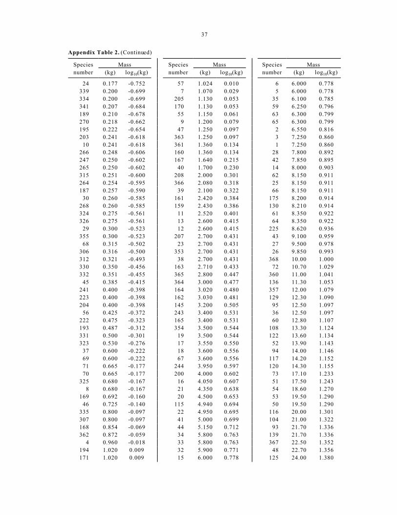
37

Appendix Table 2. (Continued)

Species

number

Mass Species

number

Mass Species

number

Mass

(kg) log10(kg) (kg) log10(kg) (kg) log10(kg)

24 0.177 -0.752 57 1.024 0.010 6 6.000 0.778

339 0.200 -0.699 7 1.070 0.029 5 6.000 0.778

334 0.200 -0.699 205 1.130 0.053 35 6.100 0.785

341 0.207 -0.684 170 1.130 0.053 59 6.250 0.796

189 0.210 -0.678 55 1.150 0.061 63 6.300 0.799

270 0.218 -0.662 9 1.200 0.079 65 6.300 0.799

195 0.222 -0.654 47 1.250 0.097 2 6.550 0.816

203 0.241 -0.618 363 1.250 0.097 3 7.250 0.860

10 0.241 -0.618 361 1.360 0.134 1 7.250 0.860

266 0.248 -0.606 160 1.360 0.134 28 7.800 0.892

247 0.250 -0.602 167 1.640 0.215 42 7.850 0.895

265 0.250 -0.602 40 1.700 0.230 14 8.000 0.903

315 0.251 -0.600 208 2.000 0.301 62 8.150 0.911

264 0.254 -0.595 366 2.080 0.318 25 8.150 0.911

187 0.257 -0.590 39 2.100 0.322 66 8.150 0.911

30 0.260 -0.585 161 2.420 0.384 175 8.200 0.914

268 0.260 -0.585 159 2.430 0.386 130 8.210 0.914

324 0.275 -0.561 11 2.520 0.401 61 8.350 0.922

326 0.275 -0.561 13 2.600 0.415 64 8.350 0.922

29 0.300 -0.523 12 2.600 0.415 225 8.620 0.936

355 0.300 -0.523 207 2.700 0.431 43 9.100 0.959

68 0.315 -0.502 23 2.700 0.431 27 9.500 0.978

306 0.316 -0.500 353 2.700 0.431 26 9.850 0.993

312 0.321 -0.493 38 2.700 0.431 368 10.00 1.000

330 0.350 -0.456 163 2.710 0.433 72 10.70 1.029

332 0.351 -0.455 365 2.800 0.447 360 11.00 1.041

45 0.385 -0.415 364 3.000 0.477 136 11.30 1.053

241 0.400 -0.398 164 3.020 0.480 357 12.00 1.079

223 0.400 -0.398 162 3.030 0.481 129 12.30 1.090

204 0.400 -0.398 145 3.200 0.505 95 12.50 1.097

56 0.425 -0.372 243 3.400 0.531 36 12.50 1.097

222 0.475 -0.323 165 3.400 0.531 60 12.80 1.107

193 0.487 -0.312 354 3.500 0.544 108 13.30 1.124

331 0.500 -0.301 19 3.500 0.544 122 13.60 1.134

323 0.530 -0.276 17 3.550 0.550 52 13.90 1.143

37 0.600 -0.222 18 3.600 0.556 94 14.00 1.146

69 0.600 -0.222 67 3.600 0.556 117 14.20 1.152

71 0.665 -0.177 244 3.950 0.597 120 14.30 1.155

70 0.665 -0.177 200 4.000 0.602 73 17.10 1.233

325 0.680 -0.167 16 4.050 0.607 51 17.50 1.243

8 0.680 -0.167 21 4.350 0.638 54 18.60 1.270

169 0.692 -0.160 20 4.500 0.653 53 19.50 1.290

46 0.725 -0.140 115 4.940 0.694 50 19.50 1.290

335 0.800 -0.097 22 4.950 0.695 116 20.00 1.301

307 0.800 -0.097 41 5.000 0.699 104 21.00 1.322

168 0.854 -0.069 44 5.150 0.712 93 21.70 1.336

362 0.872 -0.059 34 5.800 0.763 139 21.70 1.336

4 0.960 -0.018 33 5.800 0.763 367 22.50 1.352

194 1.020 0.009 32 5.900 0.771 48 22.70 1.356

171 1.020 0.009 15 6.000 0.778 125 24.00 1.380

38

Appendix Table 2. (Continued)

Species

number

Mass Species

number

Mass Species

number

Mass

(kg) log10(kg) (kg) log10(kg) (kg) log10(kg)

356 25.00 1.398 143 74.80 1.874 100 203.0 2.307

132 28.00 1.447 91 75.00 1.875 109 211.0 2.324

81 29.80 1.474 124 75.90 1.880 106 225.0 2.352

83 31.00 1.491 74 83.40 1.921 123 250.0 2.398

78 31.00 1.491 119 85.10 1.930 150 259.0 2.413

79 31.80 1.502 113 89.00 1.949 87 263.0 2.420

358 31.90 1.504 118 89.30 1.951 152 270.0 2.431

233 32.80 1.516 111 90.60 1.957 90 274.0 2.438

142 40.80 1.611 140 90.60 1.957 155 300.0 2.477

359 41.40 1.617 92 100.0 2.000 96 310.0 2.491

114 42.00 1.623 128 100.0 2.000 151 390.0 2.591

134 42.50 1.628 141 110.0 2.041 77 403.0 2.605

133 43.50 1.638 352 118.0 2.072 138 453.0 2.656

49 45.00 1.653 102 122.0 2.086 137 544.0 2.736

80 46.50 1.667 86 125.0 2.097 84 551.0 2.741

146 47.50 1.677 31 127.0 2.104 88 568.0 2.754

82 48.10 1.682 99 138.0 2.140 85 850.0 2.929

75 52.40 1.719 89 149.0 2.173 105 912.0 2.960

58 53.00 1.724 76 158.0 2.199 148 952.0 2.979

135 55.30 1.743 121 167.0 2.223 154 997.0 2.999

103 58.80 1.769 98 170.0 2.230 149 1120 3.049

131 59.40 1.774 144 171.0 2.233 153 1255 3.099

126 60.90 1.785 97 175.0 2.243 157 1810 3.258

127 65.70 1.818 156 175.0 2.243 147 2220 3.346

112 69.30 1.841 110 194.0 2.288 158 2860 3.456

101 70.00 1.845 107 197.0 2.294

39

Appendix Table 3. List of 21 species of marine fish with estimates of their population variability (coefficient of

variation and its log10 transformation) as found in Spencer and Collie (1997).

Species nameSpecies nu mber in

source document*

Variability

CV log10(CV)

Clupea harengus 12, 13, 15 0.58 -0.234

Clupea pa llasi 14 1.01 0.004

Cololabis saira 16 0.44 -0.357

Engra ulis capen sis 11 0.43 -0.367

Engraulis japonicus 9 0.60 -0.222

Engraulis mordax 10 0.65 -0.187

Gadus macrocephalus 22 0.32 -0.495

Hippo glossus sten olepis 30 0.44 -0.357

Lepido psetta biline ata 24 0.36 -0.444

Melanogrammus aeglefinus 21 0.68 -0.168

Merluccius productus 23 0.17 -0.770

Pleuronectes a spera 25 0.76 -0.119

Pleuronectes ferrugineus 26, 27 0.59 -0.233

Sardinops caeruleus 7 0.92 -0.036

Sardinops melanostictus 6 1.32 0.121

Sardinops ocellatus 8 0.88 -0.056

Sardinops sagax 5 1.10 0.041

Scomber japonicus 19, 20 0.77 -0.116

Scomber scombrus 17 0.60 -0.222

Sebastes alutus 28, 29 0.40 -0.403

Trachinus japonicus 18 0.58 -0.237

*For cases with more than one number, there were a corresponding number of measure s that were ave raged for this

table.

40

Appen dix Table 4 . List of 63 species of mamma ls of very roughly the same adult bod y mass as humans, showing

their adult body mass (kg), estimated population size (millions) and the log10 of estimated population size in millions

as based on information from Kowak (1991) and Ridgway and H arrison (1981-99).

Species nameBody mass

(kg)

Population size

(millions) log10(millions)

Acinonys jubatus 54 0.01500 -1.824

Ailuropoda melanoleuca 115 0.00100 -3.000

Antidorc as marsu pialis 39 0.60000 -0.222

Antilocapra americana 54 0.87500 -0.058

Antilope cervicap ra 38 4.00000 0.602

Arctocep halus au stralis 159 0.32200 -0.492

Arctocepha lus forsteri 160 0.03900 -1.409

Arctocep halus ga lapago ensis 150 0.00500 -2.301

Arctocep halus ga zella 140 0.37000 -0.432

Arctocephalus philippi 140 0.00100 -3.000

Arctocephalus townsendi 150 0.00050 -3.301

Arctocep halus trop icalis 165 0.11300 -0.947

Bahyrou sa babyrussa 80 0.00400 -2.398

Callorhinus ursinus 125 2.00000 0.301

Canis lupus 40 0.21000 -0.678

Canis rufus 30 0.00010 -4.000

Capra ibex 62 0.01000 -2.000

Capra pirenaica 58 0.02800 -1.553

Capra walie 100 0.00020 -3.699

Cervus elephus 200 1.00000 0.000

Connochaetes taurinus 195 3.10000 0.491

Damaliscus dorcus 110 0.15000 -0.824

Delphin us delph is 68 9.00000 0.954

Enhyd ra lutris 25 0.15000 -0.824

Felis concolor 50 0.03200 -1.495

Gorilla g orilla 135 0.05000 -1.301

Hemitragus jemlahicus 75 0.02500 -1.602

Kobus kob 125 1.00000 0.000

Kobus leche 125 0.10000 -1.000

Kobus megecerus 125 0.03500 -1.456

Lama guanicoe 110 0.57500 -0.240

Lama pacos 60 3.50000 0.544

Lasiorhin us krefftis 25 0.00004 -4.398

Lipotes vexillifer 160 0.00030 -3.523

Litorcranius walleri 40 0.07000 -1.155

Macropus fulginosus 55 1.77000 0.248

Macropus giganteus 55 8.90000 0.949

Macropus rufus 55 8.30000 0.919

41

Appendix Table 4. (Continued)

Species nameBody mass

(kg)

Population size

(millions) log10(millions)

Odocoileus verginianus 96 28.00000 1.447

Oedocoileus hemionus 60 5.50000 0.740

Oreamnoa americanus 95 0.10000 -1.000

Ovis can adensis 56 1.70000 0.230

Ovis dalli 90 0.11000 -0.959

Pan troglodytes 45 0.20000 -0.699

Panthera leo 175 0.40000 -0.398

Panthe ra tigris 175 0.10000 -1.000

Phoca caspica 100 0.56000 -0.252

Phoca groenlandica 125 2.00000 0.301

Phoca hispida 100 1.20000 0.079

Phoca siberica 100 0.04000 -1.398

Phoca vitulina 90 0.30000 -0.523

Phoco enoides dalli 100 2.15000 0.332

Platanista indi 100 0.00050 -3.301

Pongo pygmaeus 50 0.04300 -1.367

Rangifer tarandus 95 2.00000 0.301

Rupicapra pyrenaica 37 0.03100 -1.509

Rupicapra rupicapra 37 0.52300 -0.281

Saiga tatarica 47 2.00000 0.301

Stenella a ttenuata 110 22.00000 1.342

Stenella coeruleoalba 110 23.00000 1.362

Stenella lo ngirostis 110 9.00000 0.954

Ursus americans 180 0.45000 -0.347

Vicugna vicugna 50 0.12500 -0.903

42

Appen dix Table 5. List of 523 species of North American mammals with estimates of their geographic range

measured in 1,000s of square kilometers and in log10(square km) from Pagel et al. 1991 (with original data provided

by M. Pagel, University of Oxford, Oxford, England).

Species

number

Range Species

number

Range Species

number

Range

(103km2) log10(km2) (103km2) log10(km2) (103km2) log10(km2)

1 9,670.778 6.985 47 2,333.192 6.368 93 94.876 4.977

2 1,571.410 6.196 48 216.464 5.335 94 3,642.413 6.561

3 2,187.916 6.340 49 1,099.084 6.041 95 125.845 5.100

4 3,193.138 6.504 50 734.515 5.866 96 349.296 5.543

5 1,714.437 6.234 51 592.093 5.772 97 2,327.579 6.367

6 8,076.901 6.907 52 114.524 5.059 98 10,436.650 7.019

7 4,886.909 6.689 53 1,131.389 6.054 99 4,112.251 6.614

8 7,714.576 6.887 54 408.377 5.611 100 5,223.393 6.718

9 1,327.660 6.123 55 107.330 5.031 101 27.721 4.443

10 19,332.696 7.286 56 207.220 5.316 102 3,507.620 6.545

11 10,160.661 7.007 57 1,789.655 6.253 103 13,133.046 7.118

12 5,750.426 6.760 58 263.119 5.420 104 509.266 5.707

13 13,982.183 7.146 59 76.530 4.884 105 1,579.293 6.198

14 17,984.416 7.255 60 2.595 3.414 106 834.870 5.922

15 2,054.723 6.313 61 4.309 3.634 107 724.066 5.860

16 8,409.801 6.925 62 12.436 4.095 108 18.258 4.261

17 14,500.110 7.161 63 353.162 5.548 109 2,395.183 6.379

18 3,553.487 6.551 64 42.726 4.631 110 4,882.245 6.689

19 11,915.631 7.076 65 597.553 5.776 111 690.746 5.839

20 12,706.118 7.104 66 193.942 5.288 112 766.714 5.885

21 10,267.445 7.011 67 391.390 5.593 113 19.162 4.282

22 166.599 5.222 68 745.708 5.873 114 3,200.227 6.505

23 2,332.388 6.368 69 2,031.511 6.308 115 5,306.882 6.725

24 11,008.500 7.042 70 61.626 4.790 116 930.876 5.969

25 12,135.639 7.084 71 142.143 5.153 117 3,963.142 6.598

26 1,306.068 6.116 72 101.260 5.005 118 140.443 5.148

27 9,524.647 6.979 73 126.288 5.101 119 14,804.126 7.170

28 6,482.713 6.812 74 0.699 2.844 120 1,980.779 6.297

29 11,581.971 7.064 75 349.009 5.543 121 104.094 5.017

30 1,718.494 6.235 76 997.555 5.999 122 94.335 4.975

31 13,335.867 7.125 77 1,082.909 6.035 123 1,002.139 6.001

32 11,088.732 7.045 78 1,166.147 6.067 124 125.071 5.097

33 9,737.300 6.988 79 609.494 5.785 125 3,065.501 6.487

34 2,162.633 6.335 80 1,800.301 6.255 126 2,786.063 6.445

35 15,072.308 7.178 81 209.817 5.322 127 4,130.542 6.616

36 7,382.603 6.868 82 215.817 5.334 128 1,456.825 6.163

37 97.140 4.987 83 25.769 4.411 129 1,465.123 6.166

38 7,529.020 6.877 84 93.512 4.971 130 599.336 5.778

39 1.621 3.210 85 10.964 4.040 131 4,829.205 6.684

40 4.052 3.608 86 16.030 4.205 132 487.293 5.688

41 3,913.670 6.593 87 118.271 5.073 133 282.013 5.450

42 674.202 5.829 88 128.410 5.109 134 4.509 3.654

43 10,029.454 7.001 89 90.369 4.956 135 264.089 5.422

44 15,067.531 7.178 90 9.304 3.969 136 92.483 4.966

45 928.815 5.968 91 23.624 4.373 137 58.302 4.766

46 196.534 5.293 92 306.866 5.487 138 4,654.624 6.668

43

Appendix Table 5. (Continued)

Species

number

Range Species

number

Range Species

number

Range

(103km2) log10(km2) (103km2) log10(km2) (103km2) log10(km2)

139 0.950 2.978 188 1.617 3.209 237 39.565 4.597

140 115.509 5.063 189 6,896.771 6.839 238 1,805.627 6.257

141 43.174 4.635 190 553.512 5.743 239 1.394 3.144

142 149.256 5.174 191 404.282 5.607 240 3,086.579 6.489

143 4,339.389 6.637 192 361.098 5.558 241 332.793 5.522

144 10.584 4.025 193 956.530 5.981 242 128.583 5.109

145 53.857 4.731 194 2,278.309 6.358 243 428.609 5.632

146 8,440.765 6.926 195 36.649 4.564 244 7.286 3.862

147 2,820.147 6.450 196 3,422.040 6.534 245 7.501 3.875

148 197.017 5.295 197 345.716 5.539 246 15.216 4.182

149 104.827 5.020 198 878.163 5.944 247 75.007 4.875

150 5,416.801 6.734 199 1,105.274 6.043 248 648.271 5.812

151 198.682 5.298 200 11,239.258 7.051 249 0.429 2.632

152 8.350 3.922 201 938.035 5.972 250 1.929 3.285

153 64.822 4.812 202 501.638 5.700 251 15.430 4.188

154 984.299 5.993 203 184.000 5.265 252 1.714 3.234

155 91.911 4.963 204 26.946 4.430 253 387.885 5.589

156 77.389 4.889 205 3,953.100 6.597 254 161.619 5.208

157 231.715 5.365 206 245.499 5.390 255 161.919 5.209

158 817.889 5.913 207 8.324 3.920 256 60.775 4.784

159 5,811.235 6.764 208 16.880 4.227 257 1,418.094 6.152

160 340.259 5.532 209 238.373 5.377 258 0.405 2.607

161 44.088 4.644 210 25.892 4.413 259 24.310 4.386

162 375.022 5.574 211 112.021 5.049 260 292.067 5.465

163 4,285.374 6.632 212 14,483.560 7.161 261 18.485 4.267

164 528.169 5.723 213 7.595 3.881 262 25.879 4.413

165 356.870 5.553 214 76.197 4.882 263 12.939 4.112

166 7,929.817 6.899 215 504.873 5.703 264 2.958 3.471

167 12,498.145 7.097 216 13,689.319 7.136 265 2.218 3.346

168 49.804 4.697 217 2,013.211 6.304 266 514.331 5.711

169 448.832 5.652 218 42.415 4.628 267 448.776 5.652

170 401.007 5.603 219 33.537 4.526 268 6.697 3.826

171 1,253.922 6.098 220 0.233 2.367 269 184.124 5.265

172 3,956.219 6.597 221 243.421 5.386 270 24.760 4.394

173 234.308 5.370 222 136.644 5.136 271 197.333 5.295

174 788.013 5.897 223 406.769 5.609 272 13.639 4.135

175 3,189.549 6.504 224 0.149 2.173 273 277.136 5.443

176 176.278 5.246 225 1.016 3.007 274 714.539 5.854

177 107.030 5.030 226 0.618 2.791 275 863.462 5.936

178 305.589 5.485 227 0.740 2.869 276 5.602 3.748

179 10,870.202 7.036 228 35.803 4.554 277 4.749 3.677

180 625.067 5.796 229 30.733 4.488 278 2,503.359 6.399

181 4,016.231 6.604 230 13.318 4.124 279 187.820 5.274

182 3,125.474 6.495 231 107.565 5.032 280 92.199 4.965

183 4,361.341 6.640 232 30.098 4.479 281 48.980 4.690

184 528.470 5.723 233 15.344 4.186 282 392.074 5.593

185 10.838 4.035 234 29.153 4.465 283 311.023 5.493

186 230.456 5.363 235 565.780 5.753 284 2,753.152 6.440

187 375.935 5.575 236 44.217 4.646 285 885.106 5.947

44

Appendix Table 5. (Continued)

Species

number

Range Species

number

Range Species

number

Range

(103km2) log10(km2) (103km2) log10(km2) (103km2) log10(km2)

286 75.969 4.881 335 23.329 4.368 384 11.410 4.057

287 24.790 4.394 336 8.973 3.953 385 414.894 5.618

288 431.731 5.635 337 1,615.070 6.208 386 36.303 4.560

289 86.346 4.936 338 303.930 5.483 387 24.509 4.389

290 6.908 3.839 339 3,687.043 6.567 388 22.770 4.357

291 590.528 5.771 340 111.762 5.048 389 57.148 4.757

292 76.197 4.882 341 46.656 4.669 390 13.335 4.125

293 15.620 4.194 342 42.685 4.630 391 7.620 3.882

294 0.376 2.575 343 610.002 5.785 392 7.363 3.867

295 90.388 4.956 344 1,472.616 6.168 393 8.323 3.920

296 109.486 5.039 345 13,970.908 7.145 394 48.020 4.681

297 122.766 5.089 346 3,634.371 6.560 395 11.107 4.046

298 510.638 5.708 347 1,452.128 6.162 396 33.320 4.523

299 1,034.361 6.015 348 2,665.587 6.426 397 34.523 4.538

300 3,915.678 6.593 349 0.987 2.994 398 66.900 4.825

301 7,408.815 6.870 350 2.218 3.346 399 1,503.989 6.177

302 213.840 5.330 351 518.617 5.715 400 160.771 5.206

303 2,827.290 6.451 352 4.965 3.696 401 5,722.671 6.758

304 403.899 5.606 353 0.511 2.708 402 73.954 4.869

305 1,477.021 6.169 354 924.245 5.966 403 0.828 2.918

306 3,704.408 6.569 355 94.540 4.976 404 116.170 5.065

307 11,219.063 7.050 356 101.667 5.007 405 1,867.021 6.271

308 1,530.641 6.185 357 466.755 5.669 406 1,317.123 6.120

309 26.651 4.426 358 72.606 4.861 407 4,619.523 6.665

310 26.460 4.423 359 207.447 5.317 408 2.330 3.367

311 2.117 3.326 360 352.934 5.548 409 52.920 4.724

312 1.455 3.163 361 9,199.065 6.964 410 392.799 5.594

313 300.026 5.477 362 522.766 5.718 411 2,519.913 6.401

314 73.851 4.868 363 5,571.919 6.746 412 8.081 3.907

315 2,276.508 6.357 364 1,088.213 6.037 413 2,987.234 6.475

316 3,646.526 6.562 365 1,037.234 6.016 414 376.850 5.576

317 174.320 5.241 366 871.115 5.940 415 8.103 3.909

318 1,316.687 6.119 367 0.157 2.196 416 20.258 4.307

319 1,999.190 6.301 368 3.779 3.577 417 118.512 5.074

320 989.600 5.995 369 72.606 4.861 418 6.381 3.805

321 881.649 5.945 370 21.728 4.337 419 22.252 4.347

322 2,390.334 6.378 371 91.390 4.961 420 27.277 4.436

323 76.197 4.882 372 207.447 5.317 421 14.521 4.162

324 1,195.167 6.077 373 82.979 4.919 422 8.298 3.919

325 705.868 5.849 374 2.593 3.414 423 15.559 4.192

326 26.851 4.429 375 1,784.009 6.251 424 7.779 3.891

327 95.350 4.979 376 6.690 3.825 425 5.518 3.742

328 1,866.304 6.271 377 3.122 3.494 426 226.266 5.355

329 897.261 5.953 378 972.002 5.988 427 4,030.675 6.605

330 11.305 4.053 379 59.363 4.774 428 265.532 5.424

331 1,776.577 6.250 380 489.511 5.690 429 331.915 5.521

332 921.986 5.965 381 25.931 4.414 430 507.343 5.705

333 228.592 5.359 382 129.654 5.113 431 264.701 5.423

334 138.298 5.141 383 207.447 5.317 432 198.525 5.298

45

Appendix Table 5. (Continued)

Species

number

Range Species

number

Range Species

number

Range

(103km2) log10(km2) (103km2) log10(km2) (103km2) log10(km2)

433 507.092 5.705 464 76.761 4.885 495 1,383.109 6.141

434 2,966.944 6.472 465 28.623 4.457 496 193.737 5.287

435 5,927.052 6.773 466 53.332 4.727 497 322.358 5.508

436 5.543 3.744 467 36.037 4.557 498 531.080 5.725

437 91.437 4.961 468 300.530 5.478 499 3,912.196 6.592

438 457.183 5.660 469 1.855 3.268 500 3,467.540 6.540

439 26.852 4.429 470 29.891 4.476 501 5,545.246 6.744

440 41.650 4.620 471 3,969.246 6.599 502 1,715.500 6.234

441 286.469 5.457 472 7,771.747 6.891 503 6.653 3.823

442 863.318 5.936 473 7,950.383 6.900 504 1,229.200 6.090

443 346.643 5.540 474 1,747.351 6.242 505 35.520 4.550

444 22.440 4.351 475 2,605.028 6.416 506 2,438.916 6.387

445 1,694.204 6.229 476 28.747 4.459 507 458.805 5.662

446 3.746 3.574 477 4,018.504 6.604 508 50.864 4.706

447 235.299 5.372 478 679.751 5.832 509 21.183 4.326

448 33.298 4.522 479 93.006 4.969 510 12.501 4.097

449 376.061 5.575 480 222.861 5.348 511 329.685 5.518

450 9.185 3.963 481 363.812 5.561 512 1,891.591 6.277

451 5,159.040 6.713 482 681.316 5.833 513 56.176 4.750

452 1,103.715 6.043 483 3,915.084 6.593 514 80.305 4.905

453 193.118 5.286 484 49.607 4.696 515 6.142 3.788

454 127.194 5.104 485 242.351 5.384 516 5.016 3.700

455 1.184 3.073 486 96.675 4.985 517 4,010.100 6.603

456 28.884 4.461 487 53.527 4.729 518 10,446.774 7.019

457 43.289 4.636 488 310.484 5.492 519 512.831 5.710

458 102.074 5.009 489 7.512 3.876 520 1,059.952 6.025

459 18.671 4.271 490 327.023 5.515 521 7,938.016 6.900

460 615.184 5.789 491 13.349 4.125 522 2,963.526 6.472

461 370.178 5.568 492 551.580 5.742 523 184.680 5.266

462 137.037 5.137 493 15.289 4.184

463 18.036 4.256 494 6.963 3.843

46

Appen dix Table 6. Frequenc y distribution o f 19,747 species of an giosperm plants acco rding to co unts of their

chromosome number (from Masterson 1994, original data provided by J. Masterson, University of Chicago,

Chicago, IL).

Count Numberof species

Portionof species Count Number

of speciesPortion

of species Count Numberof species

Portionof species

1 0 0.0000 41 23 0.0012 81 1 0.0001

2 26 0.0013 42 76 0.0038 82 3 0.0002

3 29 0.0015 43 20 0.0010 83 1 0.0001

4 111 0.0056 44 33 0.0017 84 4 0.0002

5 265 0.0134 45 60 0.0030 85 7 0.0004

6 385 0.0194 46 25 0.0013 86 1 0.0001

7 1,157 0.0583 47 7 0.0004 87 2 0.0001

8 1,736 0.0875 48 79 0.0040 88 3 0.0002

9 1,722 0.0868 49 19 0.0010 89 0 0.0000

10 973 0.0491 50 33 0.0017 90 4 0.0002

11 1,541 0.0777 51 18 0.0009 91 2 0.0001

12 1,318 0.0664 52 24 0.0012 92 1 0.0001

13 601 0.0303 53 4 0.0002 93 1 0.0001

14 1,214 0.0612 54 48 0.0024 94 1 0.0001

15 531 0.0268 55 16 0.0008 95 2 0.0001

16 846 0.0427 56 31 0.0016 96 1 0.0001

17 548 0.0276 57 24 0.0012 97 0 0.0000

18 956 0.0482 58 17 0.0009 98 1 0.0001

19 460 0.0232 59 3 0.0002 99 1 0.0001

20 801 0.0404 60 46 0.0023 100 3 0.0002

21 429 0.0216 61 2 0.0001 101 0 0.0000

22 381 0.0192 62 9 0.0005 102 0 0.0000

23 183 0.0092 63 9 0.0005 103 1 0.0001

24 530 0.0267 64 13 0.0007 104 2 0.0001

25 180 0.0091 65 5 0.0003 105 0 0.0000

26 206 0.0104 66 7 0.0004 106 0 0.0000

27 226 0.0114 67 1 0.0001 107 0 0.0000

28 281 0.0142 68 4 0.0002 108 2 0.0001

29 90 0.0045 69 2 0.0001 109 0 0.0000

30 303 0.0153 70 12 0.0006 110 1 0.0001

31 46 0.0023 71 2 0.0001 111 0 0.0000

32 177 0.0089 72 21 0.0011 112 3 0.0002

33 81 0.0041 73 2 0.0001 113 0 0.0000

34 130 0.0066 74 4 0.0002 114 0 0.0000

35 66 0.0033 75 4 0.0002 115 0 0.0000

36 191 0.0096 76 3 0.0002 116 0 0.0000

37 19 0.0010 77 3 0.0002 117 1 0.0001

38 72 0.0036 78 4 0.0002 118 0 0.0000

39 44 0.0022 79 0 0.0000 119 0 0.0000

40 122 0.0062 80 6 0.0003 120 2 0.0001

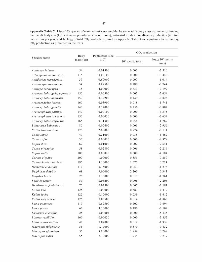
47

Appen dix Table 7. List of 63 species of mammals of very roughly the same adult body mass as humans, showing

their adult body size (kg), estimated population size (millions), estimated total carbon dioxide production (million

metric tons per year) and the log10 of total CO2 production (based on Appendix Table 4 and equations for estimating

CO2 production as presented in the text).

Species nameBody

mass (kg)

Population size

(106)

CO2 production

106 metric tonslog10(106 metric

tons)

Acinonys jubatus 54 0.01500 0.003 -2.510

Ailuropoda melanoleuca 115 0.00100 0.000 -3.440

Antidorc as marsu pialis 39 0.60000 0.097 -1.014

Antilocapra americana 54 0.87500 0.180 -0.744

Antilope cervicap ra 38 4.00000 0.633 -0.199

Arctocep halus ga lapago ensis 150 0.00500 0.002 -2.654

Arctocep halus au stralis 159 0.32200 0.149 -0.826

Arctocepha lus forsteri 160 0.03900 0.018 -1.741

Arctocep halus ga zella 140 0.37000 0.156 -0.807

Arctocephalus philippi 140 0.00100 0.000 -3.375

Arctocephalus townsendi 150 0.00050 0.000 -3.654

Arctocep halus trop icalis 165 0.11300 0.054 -1.269

Bahyrou sa babyrussa 80 0.00400 0.001 -2.956

Callorhinus ursinus 125 2.00000 0.774 -0.111

Canis lupus 40 0.21000 0.035 -1.462

Canis rufus 30 0.00010 0.000 -4.878

Capra ibex 62 0.01000 0.002 -2.641

Capra pirenaica 58 0.02800 0.006 -2.216

Capra walie 100 0.00020 0.000 -4.184

Cervus elephus 200 1.00000 0.551 -0.259

Connochaetes taurinus 195 3.10000 1.675 0.224

Damaliscus dorcus 110 0.15000 0.053 -1.278

Delphin us delph is 68 9.00000 2.205 0.343

Enhyd ra lutris 25 0.15000 0.017 -1.761

Felis concolor 50 0.03200 0.006 -2.206

Hemitragus jemlahicus 75 0.02500 0.007 -2.181

Kobus kob 125 1.00000 0.387 -0.412

Kobus leche 125 0.10000 0.039 -1.412

Kobus megecerus 125 0.03500 0.014 -1.868

Lama guanicoe 110 0.57500 0.202 -0.694

Lama pacos 60 3.50000 0.780 -0.108

Lasiorhin us krefftis 25 0.00004 0.000 -5.335

Lipotes vexillifer 160 0.00030 0.000 -3.855

Litorcranius walleri 40 0.07000 0.012 -1.939

Macropus fulginosus 55 1.77000 0.370 -0.432

Macropus giganteus 55 8.90000 1.859 0.269

Macropus rufus 55 8.30000 1.734 0.239

48

Appendix Table 7. (Continued)

Species nameBody

mass (kg)

Population size

(106)

CO2 production

106 metric tonslog10(106 metric

tons)

Odocoileus verginianus 96 28.00000 8.886 0.949

Oedocoileus hemionus 60 5.50000 1.226 0.089

Oreamnoa americanus 95 0.10000 0.031 -1.502

Ovis can adensis 56 1.70000 0.360 -0.444

Ovis dalli 90 0.11000 0.033 -1.478

Pan troglodytes 45 0.20000 0.036 -1.445

Panthera leo 175 0.40000 0.199 -0.701

Panthe ra tigris 175 0.10000 0.050 -1.303

Phoca caspica 100 0.56000 0.183 -0.737

Phoca groenlandica 125 2.00000 0.774 -0.111

Phoca hispida 100 1.20000 0.393 -0.406

Phoca siberica 100 0.04000 0.013 -1.883

Phoca vitulina 90 0.30000 0.091 -1.042

Phoco enoides dalli 100 2.15000 0.704 -0.153

Platanista indi 100 0.00050 0.000 -3.786

Pongo pygmaeus 50 0.04300 0.008 -2.078

Rangifer tarandus 95 2.00000 0.630 -0.201

Rupicapra pyrenaica 37 0.03100 0.005 -2.318

Rupicapra rupicapra 37 0.52300 0.081 -1.091

Saiga tatarica 47 2.00000 0.371 -0.430

Stenella a ttenuata 110 22.00000 7.733 0.888

Stenella coeruleoalba 110 23.00000 8.085 0.908

Stenella lo ngirostis 110 9.00000 3.164 0.500

Ursus americans 180 0.45000 0.229 -0.640

Vicugna vicugna 50 0.12500 0.024 -1.614

49

Appen dix Table 8. List of 368 species of terrestrial mamma lian primary co nsumers with measures, or estimates,

of their mean adult body mass (g), density (individuals [n] per square kilometer), energy consumption per unit area

(million joules per square kilometer per day), and log10(J/106km2day) arranged by species nu mber (as fo und with

specific names in Damuth 1987).

Species

number

Mass

(g)

Density

(n/km2)

Energy consumed

(J/106km2day) log10(J/106km2day)

1 7,250.0 25.000 92.49 1.966

2 6,550.0 51.000 175.73 2.245

3 7,250.0 74.000 273.76 2.437

4 960.0 100.000 89.85 1.953

5 6,000.0 13.500 43.75 1.641

6 6,000.0 45.000 145.82 2.164

7 1,070.0 150.000 145.40 2.163

8 680.0 255.000 179.97 2.255

9 1,200.0 15.000 15.76 1.197

10 241.0 900.000 307.30 2.488

11 2,520.0 37.000 65.33 1.815

12 2,600.0 80.000 144.37 2.159

13 2,600.0 35.000 63.16 1.800

14 8,000.0 33.000 130.79 2.117

15 6,000.0 45.000 145.82 2.164

16 4,050.0 53.000 130.44 2.115

17 3,550.0 108.000 242.38 2.384

18 3,600.0 20.000 45.33 1.656

19 3,500.0 20.000 44.44 1.648

20 4,500.0 42.000 111.28 2.046

21 4,350.0 34.000 87.97 1.944

22 4,950.0 22.500 63.73 1.804

23 2,700.0 22.500 41.69 1.620

24 177.0 250.000 68.77 1.837

25 8,150.0 230.000 923.52 2.965

26 9,850.0 112.000 513.49 2.711

27 9,500.0 30.000 134.10 2.127

28 7,800.0 0.300 1.17 0.067

29 300.0 17.500 6.97 0.843

30 260.0 17.500 6.30 0.799

31 127,00 0.0 1.800 49.41 1.694

32 5,900.0 5.100 16.33 1.213

33 5,800.0 30.000 94.94 1.977

34 5,800.0 6.200 19.62 1.293

35 6,100.0 22.000 72.12 1.858

36 12,500 .0 12.000 65.00 1.813

37 600.0 288.000 186.21 2.270

38 2,700.0 250.000 463.24 2.666

39 2,100.0 1,030.000 1,600.65 3.204

40 1,700.0 350.000 469.13 2.671

41 5,000.0 25.000 71.31 1.853

42 7,850.0 35.000 136.89 2.136

43 9,100.0 20.000 86.75 1.938

44 5,150.0 100.000 291.19 2.464

45 385.0 121.000 57.35 1.759

46 725.0 215.000 158.70 2.201

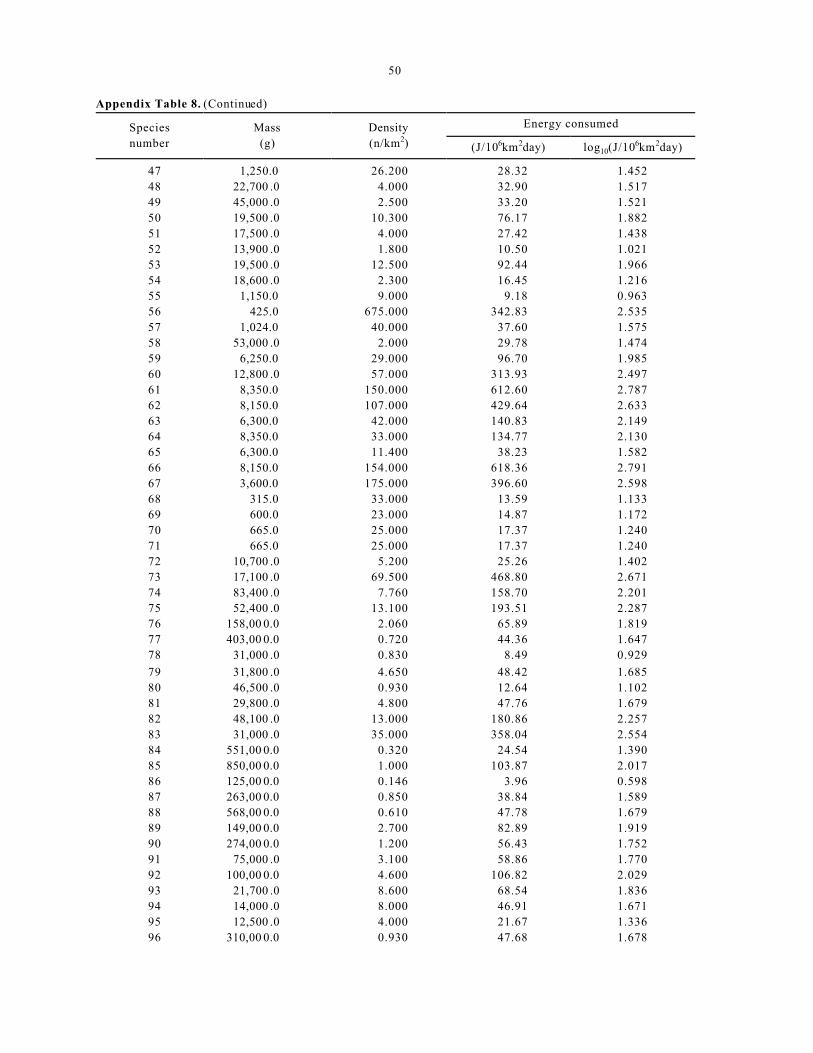
50

Appendix Table 8. (Continued)

Species

number

Mass

(g)

Density

(n/km2)

Energy consumed

(J/106km2day) log10(J/106km2day)

47 1,250.0 26.200 28.32 1.452

48 22,700 .0 4.000 32.90 1.517

49 45,000 .0 2.500 33.20 1.521

50 19,500 .0 10.300 76.17 1.882

51 17,500 .0 4.000 27.42 1.438

52 13,900 .0 1.800 10.50 1.021

53 19,500 .0 12.500 92.44 1.966

54 18,600 .0 2.300 16.45 1.216

55 1,150.0 9.000 9.18 0.963

56 425.0 675.000 342.83 2.535

57 1,024.0 40.000 37.60 1.575

58 53,000 .0 2.000 29.78 1.474

59 6,250.0 29.000 96.70 1.985

60 12,800 .0 57.000 313.93 2.497

61 8,350.0 150.000 612.60 2.787

62 8,150.0 107.000 429.64 2.633

63 6,300.0 42.000 140.83 2.149

64 8,350.0 33.000 134.77 2.130

65 6,300.0 11.400 38.23 1.582

66 8,150.0 154.000 618.36 2.791

67 3,600.0 175.000 396.60 2.598

68 315.0 33.000 13.59 1.133

69 600.0 23.000 14.87 1.172

70 665.0 25.000 17.37 1.240

71 665.0 25.000 17.37 1.240

72 10,700 .0 5.200 25.26 1.402

73 17,100 .0 69.500 468.80 2.671

74 83,400 .0 7.760 158.70 2.201

75 52,400 .0 13.100 193.51 2.287

76 158,00 0.0 2.060 65.89 1.819

77 403,00 0.0 0.720 44.36 1.647

78 31,000 .0 0.830 8.49 0.929

79 31,800 .0 4.650 48.42 1.685

80 46,500 .0 0.930 12.64 1.102

81 29,800 .0 4.800 47.76 1.679

82 48,100 .0 13.000 180.86 2.257

83 31,000 .0 35.000 358.04 2.554

84 551,00 0.0 0.320 24.54 1.390

85 850,00 0.0 1.000 103.87 2.017

86 125,00 0.0 0.146 3.96 0.598

87 263,00 0.0 0.850 38.84 1.589

88 568,00 0.0 0.610 47.78 1.679

89 149,00 0.0 2.700 82.89 1.919

90 274,00 0.0 1.200 56.43 1.752

91 75,000 .0 3.100 58.86 1.770

92 100,00 0.0 4.600 106.82 2.029

93 21,700 .0 8.600 68.54 1.836

94 14,000 .0 8.000 46.91 1.671

95 12,500 .0 4.000 21.67 1.336

96 310,00 0.0 0.930 47.68 1.678

51

Appendix Table 8. (Continued)

Species

number

Mass

(g)

Density

(n/km2)

Energy consumed

(J/106km2day) log10(J/106km2day)

97 175,00 0.0 5.480 188.28 2.275

98 170,00 0.0 12.700 427.59 2.631

99 138,00 0.0 1.420 41.32 1.616

100 203,00 0.0 7.590 289.33 2.461

101 70,000 .0 18.800 340.12 2.532

102 122,00 0.0 11.000 293.60 2.468

103 58,800 .0 1.060 16.97 1.230

104 21,000 .0 6.640 51.72 1.714

105 912,00 0.0 0.937 102.25 2.010

106 225,00 0.0 0.774 31.71 1.501

107 197,00 0.0 0.660 24.64 1.392

108 13,300 .0 17.900 101.26 2.005

109 211,00 0.0 9.110 356.80 2.552

110 194,00 0.0 1.690 62.41 1.795

111 90,600 .0 15.500 335.91 2.526

112 69,300 .0 0.150 2.69 0.431

113 89,000 .0 0.510 10.92 1.038

114 42,000 .0 1.030 13.03 1.115

115 4,940.0 111.000 313.93 2.497

116 20,000 .0 10.000 75.27 1.877

117 14,200 .0 3.530 20.91 1.320

118 89,300 .0 10.000 214.54 2.332

119 85,100 .0 12.600 261.35 2.417

120 14,300 .0 4.600 27.38 1.437

121 167,00 0.0 0.750 24.94 1.397

122 13,600 .0 1.900 10.92 1.038

123 250,00 0.0 0.360 15.88 1.201

124 75,900 .0 1.680 32.17 1.507

125 24,000 .0 5.710 48.83 1.689

126 60,900 .0 1.300 21.33 1.329

127 65,700 .0 0.270 4.67 0.670

128 100,00 0.0 2.880 66.88 1.825

129 12,300 .0 0.600 3.21 0.507

130 8,210.0 0.850 3.43 0.535

131 59,400 .0 1.460 23.55 1.372

132 28,000 .0 6.690 63.73 1.804

133 43,500 .0 0.810 10.50 1.021

134 42,500 .0 0.800 10.21 1.009

135 55,300 .0 2.840 43.56 1.639

136 11,300 .0 1.530 7.72 0.888

137 544,00 0.0 3.810 289.57 2.462

138 453,00 0.0 0.345 23.07 1.363

139 21,700 .0 7.460 59.45 1.774

140 90,600 .0 0.209 4.53 0.656

141 110,00 0.0 0.182 4.52 0.655

142 40,800 .0 10.300 127.70 2.106

143 74,800 .0 110.000 2,084.64 3.319

144 171,00 0.0 1.790 60.51 1.782

145 3,200.0 3.100 6.47 0.811

52

Appendix Table 8. (Continued)

Species

number

Mass

(g)

Density

(n/km2)

Energy consumed

(J/106km2day) log10(J/106km2day)

146 47,500 .0 3.500 48.27 1.684

147 2,220,0 00.0 0.740 150.52 2.178

148 952,00 0.0 0.840 94.46 1.975

149 1,120,0 00.0 0.093 11.72 1.069

150 259,00 0.0 3.740 169.08 2.228

151 390,00 0.0 2.570 154.73 2.190

152 270,00 0.0 1.500 69.82 1.844

153 1,255,0 00.0 6.270 855.51 2.932

154 997,00 0.0 0.120 13.94 1.144

155 300,00 0.0 0.630 31.57 1.499

156 175,00 0.0 0.800 27.49 1.439

157 1,810,0 00.0 0.490 86.39 1.936

158 2,860,0 00.0 1.090 264.72 2.423

159 2,430.0 25.600 44.06 1.644

160 1,360.0 141.000 161.66 2.209

161 2,420.0 13.000 22.31 1.349

162 3,030.0 9.970 20.03 1.302

163 2,710.0 101.000 187.63 2.273

164 3,020.0 18.600 37.28 1.571

165 3,400.0 5.840 12.72 1.104

166 154.0 558.000 139.25 2.144

167 1,640.0 131.000 171.23 2.234

168 854.0 35.400 29.30 1.467

169 692.0 544.000 388.67 2.590

170 1,130.0 588.000 592.16 2.772

171 1,020.0 68.800 64.49 1.810

172 22.0 3,450.000 220.51 2.343

173 146.0 1,590.000 382.25 2.582

174 42.0 3,300.000 331.66 2.521

175 8,200.0 25.000 100.81 2.004

176 29.1 3,626.000 281.88 2.450

177 127.0 32.000 6.98 0.844

178 20.0 1,240.000 74.14 1.870

179 36.0 949.000 85.62 1.933

180 33.0 2,550.000 216.47 2.335

181 70.0 12,400.000 1,781.96 3.251

182 103.0 862.000 162.33 2.210

183 143.0 30,900.000 7,321.51 3.865

184 71.0 257.000 37.30 1.572

185 7.0 1,550.000 44.44 1.648

186 22.5 400.000 25.97 1.414

187 257.0 21.000 7.50 0.875

188 170.0 6.500 1.74 0.240

189 210.0 111.000 34.42 1.537

190 40.0 400.000 38.85 1.589

191 40.0 1,350.000 131.12 2.118

192 40.0 286.000 27.78 1.444

193 487.0 2,040.000 1,139.74 3.057

194 1,020.0 278.000 260.60 2.416

53

Appendix Table 8. (Continued)

Species

number

Mass

(g)

Density

(n/km2)

Energy consumed

(J/106km2day) log10(J/106km2day)

195 222.0 1,250.000 402.96 2.605

196 27.0 1,160.000 85.57 1.932

197 23.0 1,890.000 124.62 2.096

198 31.0 556.000 45.18 1.655

199 28.0 4,600.000 348.08 2.542

200 4,000.0 40.300 98.32 1.993

201 30.5 250.000 20.08 1.303

202 68.7 741.000 105.10 2.022

203 241.0 247.000 84.34 1.926

204 400.0 4,200.000 2,044.55 3.311

205 1,130.0 2,470.000 2,487.48 3.396

206 88.0 1,940.000 327.23 2.515

207 2,700.0 90.000 166.76 2.222

208 2,000.0 100.000 150.19 2.177

209 5.0 985.000 22.32 1.349

210 13.5 1,980.000 89.91 1.954

211 8.2 1,170.000 37.48 1.574

212 55.0 1,429.000 173.46 2.239

213 56.0 585.000 71.91 1.857

214 60.0 504.000 65.02 1.813

215 108.0 469.000 91.30 1.960

216 145.0 1,450.000 346.92 2.540

217 72.0 950.000 139.24 2.144

218 38.5 1,209.000 114.33 2.058

219 65.0 1,310.000 178.74 2.252

220 53.0 449.000 53.11 1.725

221 145.0 205.000 49.05 1.691

222 475.0 7.000 3.84 0.585

223 400.0 40.000 19.47 1.289

224 35.0 1,610.000 142.42 2.154

225 8,620.0 3.900 16.29 1.212

226 39.0 1,700.000 162.22 2.210

227 97.0 531.000 95.88 1.982

228 26.0 1,950.000 140.10 2.146

229 69.0 293.000 41.68 1.620

230 69.0 1,090.000 155.07 2.191

231 65.0 695.000 94.83 1.977

232 63.0 91.000 12.15 1.084

233 32,800 .0 104.000 1,106.76 3.044

234 44.5 325.000 34.01 1.532

235 30.0 666.000 52.89 1.723

236 81.0 2,900.000 461.58 2.664

237 54.0 387.000 46.38 1.666

238 65.0 777.000 106.01 2.025

239 44.0 1,380.000 143.29 2.156

240 39.0 620.000 59.16 1.772

241 400.0 175.000 85.19 1.930

242 64.0 256.000 34.55 1.538

243 3,400.0 296.000 644.52 2.809

54

Appendix Table 8. (Continued)

Species

number

Mass

(g)

Density

(n/km2)

Energy consumed

(J/106km2day) log10(J/106km2day)

244 3,950.0 616.000 1,489.72 3.173

245 65.0 667.000 91.01 1.959

246 116.0 150.000 30.70 1.487

247 250.0 2,390.000 837.26 2.923

248 36.0 2,200.000 198.49 2.298

249 27.0 3,770.000 278.10 2.444

250 71.0 19,900.000 2,888.29 3.461

251 47.0 7,500.000 815.52 2.911

252 35.0 3,000.000 265.38 2.424

253 43.0 6,750.000 689.67 2.839

254 35.0 12,000.000 1,061.54 3.026

255 49.0 4,500.000 503.80 2.702

256 49.0 4,040.000 452.30 2.655

257 8.6 380.000 12.58 1.100

258 6.4 868.000 23.38 1.369

259 8.5 699.000 22.96 1.361

260 11.8 919.000 37.98 1.580

261 108.0 189.000 36.79 1.566

262 34.0 3,170.000 274.79 2.439

263 17.8 31.000 1.71 0.233

264 254.0 9,880.000 3,499.83 3.544

265 250.0 140.000 49.04 1.691

266 248.0 93.000 32.40 1.511

267 130.0 1,610.000 356.86 2.552

268 260.0 1,600.000 576.11 2.761

269 21.0 351.000 21.72 1.337

270 218.0 14,000.000 4,456.10 3.649

271 86.0 4,220.000 700.44 2.845

272 65.0 2,300.000 313.82 2.497

273 49.0 50.200 5.62 0.750

274 42.0 532.000 53.47 1.728

275 35.0 129.000 11.41 1.057

276 40.0 1,050.000 101.99 2.009

277 30.0 620.000 49.24 1.692

278 76.5 58.800 8.99 0.954

279 24.1 2,455.000 167.25 2.223

280 40.0 200.000 19.43 1.288

281 59.0 1,900.000 242.25 2.384

282 40.0 1,700.000 165.12 2.218

283 50.0 100.000 11.35 1.055

284 136.0 2,970.000 679.42 2.832

285 121.0 2,700.000 569.14 2.755

286 112.0 1,110.000 221.66 2.346

287 7.4 294.000 8.76 0.943

288 17.0 480.000 25.61 1.408

289 7.5 214.000 6.44 0.809

290 20.0 2,970.000 177.58 2.249

291 15.0 701.000 34.27 1.535

292 28.0 585.000 44.27 1.646

55

Appendix Table 8. (Continued)

Species

number

Mass

(g)

Density

(n/km2)

Energy consumed

(J/106km2day) log10(J/106km2day)

293 42.0 4,790.000 481.41 2.683

294 23.0 293.000 19.32 1.286

295 35.0 4,650.000 411.35 2.614

296 21.0 1,890.000 116.93 2.068

297 20.0 1,060.000 63.38 1.802

298 15.0 1,040.000 50.84 1.706

299 24.0 4,450.000 302.28 2.480

300 52.0 4,090.000 477.35 2.679

301 39.0 434.000 41.41 1.617

302 44.0 263.000 27.31 1.436

303 53.0 876.000 103.61 2.015

304 50.0 777.000 88.23 1.946

305 38.0 1,900.000 178.04 2.251

306 316.0 1,060.000 437.52 2.641

307 800.0 583.000 461.04 2.664

308 70.0 79.000 11.35 1.055

309 72.0 27.000 3.96 0.597

310 62.0 4,480.000 591.37 2.772

311 125.0 1,770.000 381.70 2.582

312 321.0 38.000 15.86 1.200

313 122.0 3,650.000 773.84 2.889

314 112.0 227.000 45.33 1.656

315 251.0 3,350.000 1,176.86 3.071

316 54.0 50.000 5.99 0.778

317 85.0 69.000 11.36 1.055

318 21.0 598.000 37.00 1.568

319 16.0 1,530.000 78.25 1.893

320 44.0 224.000 23.26 1.367

321 115.0 144.000 29.29 1.467

322 45.0 870.000 91.76 1.963

323 530.0 701.000 415.54 2.619

324 275.0 45.000 16.85 1.227

325 680.0 431.000 304.19 2.483

326 275.0 300.000 112.35 2.051

327 120.0 1,460.000 305.98 2.486

328 129.0 2,220.000 489.41 2.690

329 50.0 50.000 5.68 0.754

330 350.0 5,130.000 2,274.43 3.357

331 500.0 500.000 284.55 2.454

332 351.0 3,280.000 1,457.12 3.163

333 107.0 105.000 20.31 1.308

334 200.0 318.000 95.29 1.979

335 800.0 330.000 260.97 2.417

336 71.0 94.000 13.64 1.135

337 100.0 23.000 4.24 0.628

338 27.0 1,850.000 136.47 2.135

339 200.0 3,822.000 1,145.30 3.059

340 97.0 2,060.000 371.98 2.571

341 207.0 148.000 45.43 1.657

56

Appendix Table 8. (Continued)

Species

number

Mass

(g)

Density

(n/km2)

Energy consumed

(J/106km2day) log10(J/106km2day)

342 101.0 725.000 134.67 2.129

343 51.0 528.000 60.79 1.784

344 62.0 550.000 72.60 1.861

345 42.0 343.000 34.47 1.537

346 154.0 2,200.000 549.03 2.740

347 93.0 2,480.000 434.81 2.638

348 34.0 214.000 18.55 1.268

349 18.0 6,430.000 357.12 2.553

350 29.0 330.000 25.59 1.408

351 56.0 279.000 34.30 1.535

352 118,00 0.0 0.121 3.16 0.499

353 2,700.0 407.000 754.15 2.877

354 3,500.0 190.000 422.19 2.626

355 300.0 150.000 59.70 1.776

356 25,000 .0 20.800 183.03 2.263

357 12,000 .0 47.000 247.42 2.393

358 31,900 .0 15.000 156.55 2.195

359 41,400 .0 0.700 8.77 0.943

360 11,000 .0 100.000 495.32 2.695

361 1,360.0 19.600 22.47 1.352

362 872.0 125.000 105.00 2.021

363 1,250.0 83.000 89.71 1.953

364 3,000.0 511.000 1,019.33 3.008

365 2,800.0 150.000 285.11 2.455

366 2,080.0 75.000 115.77 2.064

367 22,500 .0 11.000 89.91 1.954

368 10,000 .0 20.000 92.67 1.967

57

Appen dix Table 9. List of 20 species of marine mamm als in the eastern Bering Sea ecosystem with estimates of

their total annual food consumption (103 metric tons(t)) and in log10 (103 t) from Perez and McAlister (1993).

Body

massPopulation

size

Daily energy

requireme nts

Diet energy

valueConsumption

Species (kg) (103 kcal) (kcal/g) (103 t) log10(103t)

Balaena mysticetus 46,000 148 603.1 1.80 18.1 1.257

Balaen optera a cutorostra ta 6,000 1,900 130.9 1.72 52.6 1.721

Balaenoptera physalus 49,000 500 632.3 2.00 57.5 1.760

Berard ius bairdii 8,000 209 268.1 1.20 17.0 1.230

Callorhinus ursinus 43 219,750 7.1 1.31 432.4 2.636

Delphinapterus leucas 800 10,750 47.7 1.30 143.5 2.157

Enhyd ra lutris 20 79,000 4.9 0.90 157.1 2.196

Erignathus barbatus 241 77,500 12.2 1.30 265.1 2.423

Eschrichtius robustus 18,000 2,500 298.4 1.00 271.5 2.434

Eumetopias jubatus 212 32,000 20.7 1.30 185.2 2.268

Megaptera novaeangliae 30,000 63 437.7 1.80 5.5 0.744

Mesoplod on stejnegeri 2,000 200 94.8 1.20 5.8 0.760

Orcinus orca 4,000 500 159.4 1.80 16.1 1.207

Phoca fasciata 46 66,000 3.5 1.20 70.7 1.850

Phoca hispida 34 300,500 2.8 1.20 256.7 2.409

Phoca largha 62 77,000 4.4 1.39 89.1 1.950

Phoca vitulina 49 45,000 3.7 1.40 43.3 1.637

Phocoena phocoena 50 750 6.0 1.63 1.0 -0.001

Phoco enoides dalli 95 64,100 9.6 1.33 169.0 2.228

Physeter macrocephalus 36,000 3,791 828.5 1.20 952.8 2.979

58

Appen dix Table 10. List of 20 species of marine mammals in the eastern Bering Sea ecosystem with estimates of

their total annual food and fish consumption (103 t), and in log10(103 t) transformed values of fish consumption from

Perez and McAlister (1993).

Species

Food

consumption

(103 t)

Percent fish

diet

Fish consumption

(103 t) log10(103t)

Balaena mysticetus 18.1 <0.01 0.04 -1.444

Balaen optera a cutorostra ta 52.6 60.00 31.6 1.499

Balaenoptera physalus 57.5 16.00 9.2 0.964

Berard ius bairdii 17.0 10.00 1.7 0.230

Callorhinus ursinus 432.4 67.00 289.7 2.462

Delphinapterus leucas 143.5 93.00 133.5 2.125

Enhyd ra lutris 157.1 18.00 28.3 1.452

Erignathus barbatus 265.1 23.00 61.0 1.785

Eschrichtius robustus 271.5 <0.01 0.5 -0.268

Eumetopias jubatus 185.2 76.00 140.7 2.148

Megaptera novaeangliae 5.5 29.00 1.6 0.206

Mesoplod on stejnegeri 5.8 10.00 0.6 -0.240

Orcinus orca 16.1 65.00 10.5 1.020

Phoca fasciata 70.7 54.00 38.2 1.582

Phoca hispida 256.7 85.00 218.2 2.339

Phoca largha 89.1 96.00 85.5 1.932

Phoca vitulina 43.3 75.00 32.5 1.512

Phocoena phocoena 1.0 85.00 0.8 -0.072

Phoco enoides dalli 169.0 50.00 84.5 1.927

Physeter macrocephalus 952.8 18.00 171.5 2.234

59

Appen dix Table 11. List of 20 species of predators that feed on walleye pollock (Theragra chalcogramma) in the

eastern Bering Sea showing the percent of the estimated standing stock biomass of pollock that is consumed by each

predator species annually, along with the log10 transformation (from Livingston 1993, and Livingston, personal

comm., Alaska Fisheries Science Center, Seattle, WA).

SpeciesPercent of pollock

biomass consumedlog10(percent biomass)

Callorhinus ursinus 1.460 0.164

Eumetopias jubatus 0.594 -0.226

Phoca vitulina 0.187 -0.729

Phoca larga 0.117 -0.931

Phoca hispida 0.299 -0.525

Erignathus barbatus 0.036 -1.439

Uria aalge 0.912 -0.040

Uria lom via 1.294 0.112

Fulma rus glacia lis 0.276 -0.559

Ocean odrom a furcata 0.021 -1.673

Larus trida ctyla 0.127 -0.895

Fratercu la cornicu lata 0.021 -1.673

Lunda cirrhata 0.233 -0.632

Gadus macrocephalus 2.143 0.331

Atheresthes stomias 0.140 -0.853

Hippoglossoides elassodon 0.019 -1.710

Pleuronectes bilineatus 0.000 -4.732

Pleuronectes asper 0.011 -1.972

Reinhardtius hippoglossoides 0.010 -2.002

Hippo glossus sten olepis 0.006 -2.192

RECENT TECHNICAL MEMORANDUMS

Copies of this and other NOAA Technical Memorandums are available from theNational Technical Information Service, 5285 Port Royal Road, Springfield, VA 22167(web site: www.ntis.gov). Paper and microfiche copies vary in price.

AFSC-

108 HILL, P. S., J. L. LAAKE, and E. MITCHELL. 1999. Results of a pilot program to document interactionsbetween sperm whales and longline vessels in Alaska waters, 42 p. NTIS number pending.

107 MOORE, S. E., M. E. DAHLHEIM, K. M. STAFFORD, C. G. FOX, H. W. BRAHAM, M. A. MCDONALD,and J. THOMASON. 1999. Acoustic and visual detection of large whales in the eastern north PacificOcean, 27 p. NTIS number pending.

106 SINCLAIR, E.H., and B. W. ROBSON. (editors). 1999. Fur seal investigations, 1997, 111 p. NTIS No.PB2000-100223.

105 MURPHY, J. M., A. L. J. BRASE, and J. A. ORSI. 1999. Survey of juvenile Pacific salmon in the northernregion of southeastern Alaska, May-October 1997, 40 p. NTIS No. PB99-175630.

104 SMITH, K. R., and R. A. MCCONNAUGHEY. 1999. Surficial sediments of the eastern Bering Seacontinental shelf: EBSSED database documentation, 41 p. NTIS No. PB2000-100938.

103 RUGH, D. J., M. M. MUTO, S. E. MOORE, and D. P. DEMASTER. 1999. Status review of the easternnorth Pacific stock of gray whales, 93 p. NTIS No. PB99-172678.

102 BUCKLEY, T. W., G. E. TYLER, D. M. SMITH, and P. A. LIVINGSTON. 1999. Food habits of somecommercially important groundfish off the coasts of California, Oregon, Washington, and BritishColumbia, 173 p. NTIS No. PB99-166563.

101 MCELDERRY, H., W. A. KARP, J. TWOMEY, M. MERKLEIN, V. CORNISH, and M. SAUNDERS. 1999.Proceedings of the first biennial Canada/U.S. observer program workshop, 113 p. NTIS No. PB99-146482.

100 SEASE, J. L., and T. R. LOUGHLIN. 1999. Aerial and land-based surveys of Steller sea lions(Eumetopias jubatus) in Alaska, June and July 1997 and 1998, 61 p. NTIS No. PB99-140618.

99 SEASE, J. L., J. M. STRICK, R. L. MERRICK, and J. P. LEWIS. 1999. Aerial and land-based surveysof Steller sea lions (Eumetopias jubatus) in Alaska, June and July 1996, 43 p. NTIS No. PB99-134462.

98 LAUTH, R. R. 1999. The 1997 Pacific West Coast upper continental slope trawl survey of groundfishresources off Washington, Oregon, and California: Estimates of distribution, abundance, and lengthcomposition, 284 p. NTIS No. PB99-133043.

97 HILL, P. S., and D. P. DEMASTER. 1998. Alaska marine mammal stock assessments, 1998, 166 p. NTISNo. PB99-130791.

96 WING, B. L., M. M. MASUDA, C. M. GUTHRIE III, and J. H. HELLE. 1998. Some size relationships andgenetic variability of Atlantic salmon (Salmo salar) escapees captured in Alaska fisheries, 1990-95, 32 p.NTIS No. PB99-118697.

95 ORR, J. W., M. A. BROWN, and D. C. BAKER. 1998. Guide to rockfishes (Scorpaenidae) of the generaSebastes, Sebastolobus, and Adelosebastes of the northeast Pacific Ocean, 46 p. NTIS No. PB99-114217.

94 THROWER, F., R. MARTIN, and R. HEINTZ. 1998. Effect of seawater entry date on 24-hour plasmasodium concentration and survival of juvenile spring chinook salmon (Oncorhynchus tshawytscha) rearedin marine net-pens, 18 p. NTIS No. PB98-173545.