constructing endomorphism rings of large finite global...
TRANSCRIPT
Constructing Endomorphism Rings of Large Finite GlobalDimension
by
Ali Mousavidehshikh
A thesis submitted in conformity with the requirementsfor the degree of Doctor of PhilosophyGraduate Department of Mathematics
University of Toronto
c© Copyright 2016 by Ali Mousavidehshikh

Abstract
Constructing Endomorphism Rings of Large Finite Global Dimension
Ali Mousavidehshikh
Doctor of Philosophy
Graduate Department of Mathematics
University of Toronto
2016
For a numerical semigroup H with generators α1, α2, ..., αs, let R be the subring of the
ring of formal power series k[[t]] (where k is a field of characteristic zero) with generators
tα1 , tα2 , ..., tαs . More precisely,
R := k[[tα1 , tα2 , ..., tαs ]] =
{∑i≥0
aiti : ai ∈ k, i ∈ H
}
For R 6= k[[t]], we construct ascending chains of rings R = R1 ( R2 ( ... ( Rl =
k[[t]], and we then consider E = EndR1
(⊕li=1Ri
). Our arguments show that the global
dimension of E depends on R1 and the way we construct our ascending chain. This
leads to an investigation of two types of constructions for our ascending chain, which
we call the “greedy” and “lazy” constructions. In the “greedy” construction we choose
Ri+1 as the endomorphism ring of the radical of Ri. In the “lazy” (or, as Iyama calls it,
saturated) construction we choose Ri+1 so that dimk(Ri+1/Ri) = 1 and the conductor of
Ri+1 is strictly larger than that of Ri. We introduce a special family of rings {Ri1 : i ∈ N},
thinking of each as the beginning of an ascending chain and we let {Ei : i ∈ N} be the
set of corresponding endomorphism rings.
This thesis consists of three main results. Firstly, if for each i our chain is constructed
via the “lazy” construction, then {gl. dim(Ei) : i ∈ N} is an unbounded set. Secondly,
under some additional assumptions on the set {Ri1 : i ∈ N} we compute the precise values
in the set {gl. dim(Ei) : i ∈ N}. Thirdly, if for each i the chain is constructed via the
“greedy” construction, then gl. dim(Ei) = 2 for all i.
ii

Dedication
Dedicated to my loving parents Zahra and Seyedalizamen whose support and constant
encouragement has gotten me here.
It is also dedicated to my sister Maryam and my brother Mahmoud who always keep
me calm and focused.
iii

Acknowledgements
I would first like to thank my supervisor, Ragnar-Olaf Buchweitz, for his patience, ex-
pertise, and encouragement. It has been an honour to be your student. I would also
like to thank my Ph.D committee members, professors Marco Gualtieri and Joe Repka,
who on a yearly basis would take time out of their busy schedule to meet with me, and
provide insight and feedback on my research. I would also like to thank Osamu Iyama
for being my external referee. In addition, I would like to thank all the members of the
homological seminar for all the fun and knowledgeable conversations.
It is very hard for me to put into words the affection that I feel for the staff at the
mathematics department at the University of Toronto. To put it kindly, their support,
generosity and smile makes the department an extremely comfortable place. I would
like to send a special thanks to Marie Bachtis, Ida Bullat, Rajni Lala, Jemima Merisca,
Patrina Seepersaud, and Aisha Sharif. Ida, you are sourly missed but never forgotten.
There are several people in the department with whom I had discussions that con-
tributed to this work or my overall understanding. In particular, I am grateful to
Robin Chhabra, Peter Crooks, Payman Eskandari, Brandon Hanson, Dave Reiss and
Ben Rifkind for their time and support. Also a big thanks to professors Shay Fuchs
and Abe Iglefeld for all the enlightening conversations. My warmest thanks also go to
anybody who took time out of their day to have a beer or two with me, the list is too
long to put here.
Finally, I would like to thank my parents, brother and sister for all their support.
I would also like to thank my close friends from high school, Jagdeep Jodha, Paul Pa-
trocinio, Ajay Sharma, and Mark Wright.
iv
Contents
1 Introduction and Background 1
1.1 Introduction . . . . . . . . . . . . . . . . . . . . . . . . . . . . . . . . . . 1
1.2 Frobenius Number . . . . . . . . . . . . . . . . . . . . . . . . . . . . . . 4
1.3 Minimal Projective Resolution and Global Dimension . . . . . . . . . . . 4
1.4 Krull-Remak-Schmidt Categories . . . . . . . . . . . . . . . . . . . . . . 6
1.5 Mapping Cone . . . . . . . . . . . . . . . . . . . . . . . . . . . . . . . . . 7
1.6 Outline of this thesis . . . . . . . . . . . . . . . . . . . . . . . . . . . . . 9
2 Main Objects and Tools 11
2.1 Conventions, Definitions, and Notations . . . . . . . . . . . . . . . . . . . 11
2.2 The Construction . . . . . . . . . . . . . . . . . . . . . . . . . . . . . . . 15
2.3 A Presentation of a Ring, an Image and Kernel of a Map . . . . . . . . . 23
2.4 Structure of E . . . . . . . . . . . . . . . . . . . . . . . . . . . . . . . . . 32
2.5 Family of Starting Rings . . . . . . . . . . . . . . . . . . . . . . . . . . . 35
2.6 The symbol d e . . . . . . . . . . . . . . . . . . . . . . . . . . . . . . . . 39
3 “Lazy” Construction 44
3.1 The Construction . . . . . . . . . . . . . . . . . . . . . . . . . . . . . . . 44
3.2 Special Rings I . . . . . . . . . . . . . . . . . . . . . . . . . . . . . . . . 47
3.3 Minor Results I . . . . . . . . . . . . . . . . . . . . . . . . . . . . . . . . 60
3.4 gl. dim(E) for l = 1, 2, 3, 4, 5 . . . . . . . . . . . . . . . . . . . . . . . . . 67
3.5 Constructing Endomorphism Rings of Large Global Dimension . . . . . . 69
3.5.1 Minor Results II . . . . . . . . . . . . . . . . . . . . . . . . . . . 70
3.5.2 Lower Bound for gl. dim(Ei) . . . . . . . . . . . . . . . . . . . . . 75
3.5.3 The Module M ′ . . . . . . . . . . . . . . . . . . . . . . . . . . . . 89
3.5.4 Global Dimension . . . . . . . . . . . . . . . . . . . . . . . . . . . 91
v
4 “Greedy” Construction 116
4.1 The Construction . . . . . . . . . . . . . . . . . . . . . . . . . . . . . . . 116
4.2 Special Rings II . . . . . . . . . . . . . . . . . . . . . . . . . . . . . . . . 117
4.3 Minor Results III . . . . . . . . . . . . . . . . . . . . . . . . . . . . . . . 125
4.4 gl. dim(Ei) = 2 . . . . . . . . . . . . . . . . . . . . . . . . . . . . . . . . 128
5 Examples and Open Questions 147
5.1 Examples . . . . . . . . . . . . . . . . . . . . . . . . . . . . . . . . . . . 148
5.2 Open Questions . . . . . . . . . . . . . . . . . . . . . . . . . . . . . . . . 155
Bibliography 156
vi

Chapter 1
Introduction and Background
1.1 Introduction
Let N0 be the set of non-negative integers. A setH ⊆ N0 is called a numerical semigroup
if it satisfies the following three properties;
(a) 0 ∈ H,
(b) If x, y ∈ H then x+ y ∈ H,
(c) H contains all but a finite number of the non-negative integers.
Given A = {α1, α2, ..., αs} ⊆ N, let
〈A〉 = 〈α1, α2, ..., αs〉 := {x1α1 + ...+ xsαs : xi ∈ N0}
We call A a generating set for 〈α1, α2, ..., αs〉. The set A is called a minimal generating
set if no proper subsets of A is a generating set. It is a standard fact that 〈A〉 forms
a numerical semigroup if and only if gcd(A) = 1, and every numerical semigroup arises
this way. Furthermore, every numerical semigroup has a unique minimal generating set,
and this set has finitely many elements (see [18] or [19]).
Fix a field k of characteristic zero and a numerical semigroup H with generators
α1, α2, . . . , αs, written in ascending order. Let R be a ring of formal power series over k
with topological generators
tα1 , tα2 , ..., tαs
1

Chapter 1. Introduction and Background 2
That is,
R := k[[tα1 , tα2 , ..., tαs ]] =
{∑i≥0
aiti : ai ∈ k, i ∈ H
}
In this case, we say that R is the ring of formal power series associated to H. There is
a 1-1 correspondence between numerical semigroups and the rings of formal power series
associated to them. Given such a ring, a natural question to ask is: can we construct an
R-module M such that the endomorphism ring of M , denoted EndR(M) has finite global
dimension? What is the minimum value (or maximum value) for the global dimension?
Can we actually compute the global dimension?
We begin with an essential property regarding reduced complete local Noetherian
rings of Krull dimension one.
Theorem 1.1.1. Let (R,m, k) be a reduced complete local Noetherian ring of (Krull)
dimension one with integral closure R̃ and total quotient ring R (obtained by inverting
all non-zero divisors of R). Then R ⊆ EndR(m) ⊆ R̃ (up to canonical identification).
Moreover, R = EndR(m) if and only if R = R̃ (see [4, 5, 21]).
Note that R is a product of finitely many fields, and R̃ is a product of finitely many
discrete valuation rings. Since R is complete and reduced, R̃ is a finitely generated
R-module (see [12], Theorem 11.7).
Given a numerical semigroupH withR being the ring of formal power series associated
to it, the preceding theorem allows us to construct an ascending chain of rings with R
being the beginning of this chain;
R = R1 ( R2 ( . . . ( Rl = k[[t]] (1.1)
We define
M :=l⊕
i=1
Ri, E := EndR1(M)
This thesis is concerned with computing the global dimension of E. If we assume
Ri+1 ⊆ EndR1(mi) in the ascending chain of rings given in (1.1), where mi is the maximal
ideal of Ri, then gl. dim(E) ≤ l (see [6], [7] example 2.2.3(2), and [11]). The following
proposition takes care of l = 1.
Proposition 1.1.2. If H = N0 and R is the ring of formal power series associated to
H, then gl. dim(R) = dim(R) = 1.

Chapter 1. Introduction and Background 3
Proof. It follows that R = k[[t]], in which case R is a regular local Noetherian ring and
the result follows.
The following theorem reduces our problem to computing the projective dimension of
the simple E-modules.
Theorem 1.1.3. Let A be an associative ring with unit that is module finite over a local
Noetherian ring R in its centre. Then the global dimension of A equals the supremum of
the projective dimensions of the simple A-modules (see [3], Proposition 6.7 page 125 or
[13], 7.1.14).
The preceding theorem leads us to investigate methods for coming up with minimal
projective resolutions for the simple E-modules. The following theorem gives us a helping
hand in this matter.
Theorem 1.1.4. Let R be a complete local Noetherian commutative ring, and A be a
R-algebra which is finitely generated as an R-module. Then A = A/J(A) is a semi-simple
Artinian ring, where J(A) is the Jacobian radical of A. Suppose that 1 = e1 + ...+ en is
a decomposition of 1 ∈ A into orthogonal primitive idempotents in A. Then
A =n⊕i=1
eiA
is a decomposition in indecomposable right ideals of A and
A =n⊕i=1
eiA
is a decomposition of A into minimal right ideals. Moreover, eiA ∼= ejA if and only if
eiA ∼= ejA (see [15] Theorem 6.18, 6.21 and Corollary 6.22).
This theorem says that the indecomposable summands of A are of the form Pi = eiA.
By definition, the Pi are the indecomposable projective modules over A. The modules
Si = Pi/J(A) are the simple modules over A (as well as over the semi simple algebra A)
and Pi → Si → 0 is a projective cover.
The remainder of this chapter focuses on the necessary background required for this
thesis. Unless otherwise stated, k will be a field of characteristic zero and H will be a
numerical semigroup with H 6= N0, the set of non-negative integers. This is equivalent
to l ≥ 2 in the ascending chain of rings given in (1.1).
Chapter 1. Introduction and Background 4
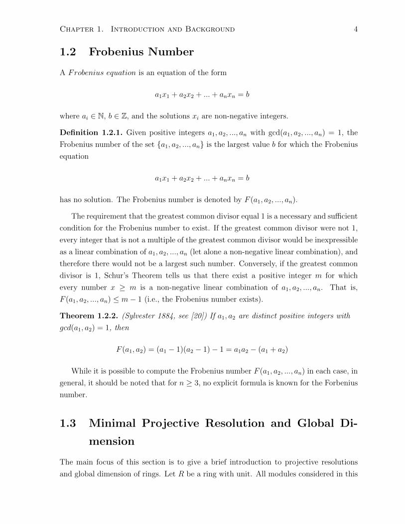
1.2 Frobenius Number
A Frobenius equation is an equation of the form
a1x1 + a2x2 + ...+ anxn = b
where ai ∈ N, b ∈ Z, and the solutions xi are non-negative integers.
Definition 1.2.1. Given positive integers a1, a2, ..., an with gcd(a1, a2, ..., an) = 1, the
Frobenius number of the set {a1, a2, ..., an} is the largest value b for which the Frobenius
equation
a1x1 + a2x2 + ...+ anxn = b
has no solution. The Frobenius number is denoted by F (a1, a2, ..., an).
The requirement that the greatest common divisor equal 1 is a necessary and sufficient
condition for the Frobenius number to exist. If the greatest common divisor were not 1,
every integer that is not a multiple of the greatest common divisor would be inexpressible
as a linear combination of a1, a2, ..., an (let alone a non-negative linear combination), and
therefore there would not be a largest such number. Conversely, if the greatest common
divisor is 1, Schur’s Theorem tells us that there exist a positive integer m for which
every number x ≥ m is a non-negative linear combination of a1, a2, ..., an. That is,
F (a1, a2, ..., an) ≤ m− 1 (i.e., the Frobenius number exists).
Theorem 1.2.2. (Sylvester 1884, see [20]) If a1, a2 are distinct positive integers with
gcd(a1, a2) = 1, then
F (a1, a2) = (a1 − 1)(a2 − 1)− 1 = a1a2 − (a1 + a2)
While it is possible to compute the Frobenius number F (a1, a2, ..., an) in each case, in
general, it should be noted that for n ≥ 3, no explicit formula is known for the Forbenius
number.
1.3 Minimal Projective Resolution and Global Di-
mension
The main focus of this section is to give a brief introduction to projective resolutions
and global dimension of rings. Let R be a ring with unit. All modules considered in this
Chapter 1. Introduction and Background 5
thesis will be right R-modules (if R is not commutative). However, similar definitions
and results can be stated for left R-modules. The set of all right R-modules is denoted
by ModR, and the set of all left R-modules is denoted by RMod. For a more “in-depth”
look we refer the reader to [8, 9, 17].
Suppose M is a submodule of N . We say that M is a superfluous submodule of N
if for any other submodule H of N ,
M +H = N ⇒ H = N
That is, M is “extremely small” relative to N .
Let M and P be R-modules, with P a projective R-module. Then, (P, f) is called a
projective cover for M if f : P → M is a superfluous epimorphism. That is, f is an
epimorphism and ker f is a superfluous submodule of P . Another common convention is
to say P →M → 0 is a projective cover when the map P →M is understood.
A projective resolution of an R-module M is an exact sequence
· · · → P2d2−→ P1
d1−→ P0ε−→M → 0
in which each Pi is a projective R-module. A free resolution of M is a projective
resolution in which each Pi is free; a flat resolution is an exact sequence in which each
Pi is flat. A finite projective resolution of M is a projective resolution of the following
form;
0→ Pndn−→ Pn−1
dn−1−→ ...d1−→ P0
ε−→M → 0
That is, there exists a natural number n such that Pi = 0 for all i ≥ n. In this case, n
is called the length of the projective resolution. A finite projective resolution is said to
be minimal if (Pi, di) is a projective cover for Im(di) for i = 1, 2, ..., n and (P0, ε) is a
projective cover for M . The length of a minimal projective resolutions is unique.
Remark 1.3.1. It is well known that a projective resolution is minimal if and only if
Im(di) ⊆ J(Pi−1) for i = 1, 2, ..., n and P0ε→M → 0 is a projective cover.
IfM is a rightR-module andM has a finite projective resolution, the projective dimension
of M , denoted pdR(M), is defined to be the minimal length among all finite projective
resolutions of M . If no finite projective resolution exists for M then pdR(M) =∞. The
right global dimension of a ring R is
gl. dim(R) = sup{pdR(M) : M ∈ModR}
Chapter 1. Introduction and Background 6
A similar definition is given for left modules and the left global dimension of a ring.
It is well known that the projective resolution of a module M is equal to the length of
any of its minimal projective resolutions, provided it has a minimal projective resolution
(recall that they all have the same length).
1.4 Krull-Remak-Schmidt Categories
In this section we introduce Krull-Remak-Schmidt Categories and give a summary of
some of the results related to them. For an “in-depth” look at these categories we refer
the reader to [10] or any book on this subject.
Definition 1.4.1. A category A is called additive if
(1) each morphism set HomA(X, Y ) is an (additive) abelian group for every X, Y ∈obj(A),
(2) the composition maps
HomA(Y, Z)× HomA(Y, Z)→ HomA(X,Z)
are bilinear, i.e., the distributive laws hold,
(3) A has a zero object,
(4) A has finite products and finite coproducts.
Definition 1.4.2. A category A is called an abelian category if it is an additive category
such that
(1) every morphism has a kernel and cokernel,
(2) every monomorphism is a kernel and every epimorphism is a cokernel.
An additive category is called Krull-Remak-Schmidt if every object decomposes
into a finite direct sum of objects having local endomorphism rings. An object is called
indecomposable if it is not isomorphic to a direct sum of two non-zero objects.
Theorem 1.4.3. (Krull-Remak-Schmidt theorem) Let A be a Krull-Remak-Schmidt Cat-
egory. Then
(1) An object is indecomposable if and only if its endomorphism ring is local.
(2) Every object is isomorphic to a finite direct sum of indecomposable objects.
(3) If
r⊕i=1
Xi∼=
s⊕j=1
Yj

Chapter 1. Introduction and Background 7
where Xi, Yj are indecomposable objects in A, then r = s and there exists a permutation
σ such that Xσ(i)∼= Yi for all i.
Proposition 1.4.4. For a ring R the following are equivalent.
(1) The category of finitely generated projective right (left) R-modules is a Krull-Remak-
Schmidt category.
(2) The module R admits a decomposition R = P1 ⊕ P2 ⊕ . . .⊕ Pr such that each Pi is a
projective right (left) R-module having a local endomorphism ring.
(3) Every simple right (left) R-module admits a projective cover.
(4) Every finitely generated right (left) R-module admits a projective cover.
Proof. See Proposition 4.1 in [10].
Example 1.4.5. Here are some examples of Krull-Remak-Schmidt categories details of
which can be found in [1, 15].
(a) An abelian category in which every object has finite length.
(b) Let R be a commutative complete local Noetherian ring. The category of finitely-
generated modules over R is a Krull-Schmidt category.
(c) The category of coherent sheaves on a projective variety.
(d) The category of finitely generated modules over a finite R-algebra, where R is a
commutative Noetherian complete local ring (this is a generalization of (b)).
1.5 Mapping Cone
Let A be an additive category. A chain complex in A is a sequence of objects and
morphisms in A, called differentials,
(A•, d•) = · · · An−1 An An+1 · · ·dn dn+1
such that the composite of adjacent morphisms is zero;
dndn+1 = 0 for all n ∈ Z
We call n the homological degree of An, abbreviated H.D. If (A•, d•) and (B•, g•) are
two chain complexes, then a chain map
f = f• = (A•, d•)→ (B•, g•)
Chapter 1. Introduction and Background 8
is a sequence of morphisms fn : An → Bn for all n ∈ Z making the following diagram
commute:
· · · An−1 An An+1 · · ·
· · · Bn−1 Bn Bn+1 · · ·
dn dn+1
gn gn+1
fn−1 fn fn+1
If the indices are increasing in the above complex and commutative diagram, we call the
complex and map a cochain complex and cochain map, respectively (in this case the
convention is to use superscripts instead of subscripts for the indices).
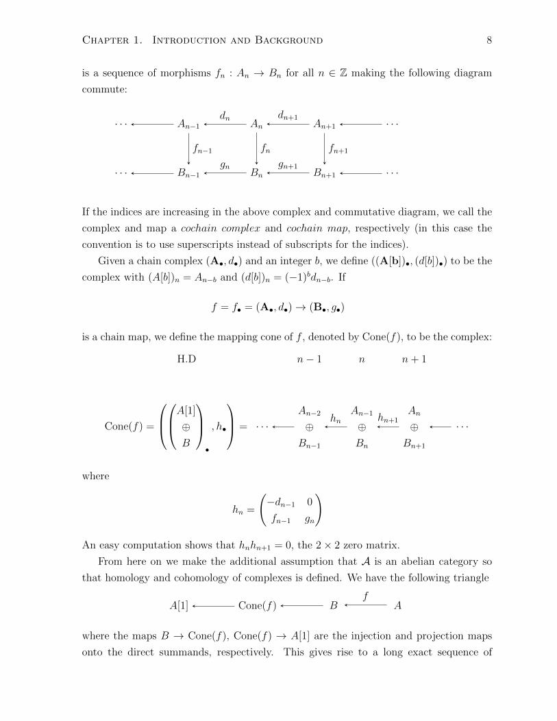
Given a chain complex (A•, d•) and an integer b, we define ((A[b])•, (d[b])•) to be the
complex with (A[b])n = An−b and (d[b])n = (−1)bdn−b. If
f = f• = (A•, d•)→ (B•, g•)
is a chain map, we define the mapping cone of f , denoted by Cone(f), to be the complex:
H.D n− 1 n n+ 1
Cone(f) =
A[1]
⊕B
•
, h•
= · · ·An−2
⊕Bn−1
An−1
⊕Bn
An
⊕Bn+1
· · ·hn hn+1
where
hn =
(−dn−1 0
fn−1 gn
)
An easy computation shows that hnhn+1 = 0, the 2× 2 zero matrix.
From here on we make the additional assumption that A is an abelian category so
that homology and cohomology of complexes is defined. We have the following triangle
A[1] Cone(f) B Af
where the maps B → Cone(f), Cone(f) → A[1] are the injection and projection maps
onto the direct summands, respectively. This gives rise to a long exact sequence of
Chapter 1. Introduction and Background 9
homology groups (for more details see chapter 6 in [17] or any book on triangulated
categories such as chapter 1 in [14])
· · · Hi−1(B) Hi−1(A) Hi(Cone(f)) Hi(B) Hi(A) · · ·
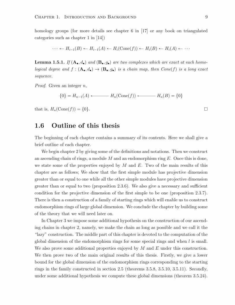
Lemma 1.5.1. If (A•, d•) and (B•, g•) are two complexes which are exact at each homo-
logical degree and f : (A•, d•) → (B•, g•) is a chain map, then Cone(f) is a long exact
sequence.
Proof. Given an integer n,
{0} = Hn−1(A) Hn(Cone(f)) Hn(B) = {0}
that is, Hn(Cone(f)) = {0}.
1.6 Outline of this thesis
The beginning of each chapter contains a summary of its contents. Here we shall give a
brief outline of each chapter.
We begin chapter 2 by giving some of the definitions and notations. Then we construct
an ascending chain of rings, a module M and an endomorphism ring E. Once this is done,
we state some of the properties enjoyed by M and E. Two of the main results of this
chapter are as follows; We show that the first simple module has projective dimension
greater than or equal to one while all the other simple modules have projective dimension
greater than or equal to two (proposition 2.3.6). We also give a necessary and sufficient
condition for the projective dimension of the first simple to be one (proposition 2.3.7).
There is then a construction of a family of starting rings which will enable us to construct
endomorphism rings of large global dimension. We conclude the chapter by building some
of the theory that we will need later on.
In Chapter 3 we impose some additional hypothesis on the construction of our ascend-
ing chains in chapter 2, namely, we make the chain as long as possible and we call it the
“lazy” construction. The middle part of this chapter is devoted to the computation of the
global dimension of the endomorphism rings for some special rings and when l is small.
We also prove some additional properties enjoyed by M and E under this construction.
We then prove two of the main original results of this thesis. Firstly, we give a lower
bound for the global dimension of the endomorphism rings corresponding to the starting
rings in the family constructed in section 2.5 (theorems 3.5.8, 3.5.10, 3.5.11). Secondly,
under some additional hypothesis we compute these global dimensions (theorem 3.5.24).

Chapter 1. Introduction and Background 10
In Chapter 4 we impose restrictions on the chain constructed in chapter 2 to make
the length of it as short as possible, we call it the “greedy” construction. The middle
part of this chapter is analogous to that of the preceding chapter but everything is done
under the “greedy” construction. We then prove the third main original result of this
thesis: for the family of starting rings constructed in section 2.5 the global dimension of
the endomorphism rings corresponding to the starting rings in the family is two (theorem
4.4.7).
In Chapter 5 we give an example which illustrates the possible values for the global
dimension of E when our starting ring is fixed. We conclude the chapter by discussing
some open questions related to this thesis which could be subject of future research.

Chapter 2
Main Objects and Tools
In this chapter we introduce the main objects studied in this thesis and the tools needed
to understand some of their elementary properties. More specifically, in section 2.1 we
introduce the notation and definitions used throughout this thesis. Section 2.2 focuses
on constructing endomorphism rings. We view these endomorphism rings as rings of
matrices and in section 2.4 we describe the entries of these matrices. In section 2.5 we
focus on a family of rings which will enable us to construct a set of endomorphism rings
whose global dimensions are arbitrarily large (but finite). We conclude this chapter by
introducing two of the most used tools in this thesis.
2.1 Conventions, Definitions, and Notations
We begin with some useful definitions regarding numerical semigroups and the rings
associated to them.
Definition 2.1.1. Let R be a ring of formal power series associated to a numerical
semigroup H. Recall that every numerical semigroup has a unique minimal generating
set. Let {α1, α2, ..., αs} be the minimal generating set for H. Let m be the maximal ideal
of R. We define
e(R) = min{n ∈ N| tn ∈ R}
C(R) = min{a ∈ N| tb ∈ R for all b ≥ a}
Γ(R) = {β ∈ N| tβ ∈ R and β ≤ C(R)}
Λ(R) = {β ∈ N| β < C(R) and β ∈ {α1, α2, ..., αs}}
We call e(R) the multiplicity of R. We also define e(m) = e(R),Γ(m) = Γ(R), and
11

Chapter 2. Main Objects and Tools 12
Λ(m) = Λ(R). We will always assume the elements in Γ(R) and Λ(R) are written in
ascending order. Also, all of the above definitions can be given in terms of the numerical
semigroup H;
e(H) = min{n ∈ N| n ∈ H}
C(H) = min{a ∈ N| b ∈ H for all b ≥ a}
Γ(H) = {β ∈ N| β ∈ H and β ≤ C(H)}
Λ(H) = {β ∈ N| β < C(H) and β ∈ {α1, α2, ..., αs}}
Notation 2.1.2. Given a ring R, the principal ideal generated by tn in R is denoted by
tnR.
Let R be a ring and A a subring of R such that R is integral over A. Then the
annihlator of the A-module R/A is called the conductor of A in R, denoted by c(R/A).
Explicitly, c(R/A) consists of elements a ∈ A such that aR ⊆ A. This is the largest ideal
of A that is also an ideal of R. If R is a subring of the total ring of fractions of A, then
we have the following identification:
c(R/A) = HomA(R,A)
A consequence of our definition are the following results, which we record for future
reference.
Lemma 2.1.3. Let H be a numerical semigroup with generators α1, α2, ..., αs and R be
the ring associated to H. Let m be the maximal ideal of R.
(a) 1 ≤ e(R) <∞, 1 ≤ C(R) <∞(b) e(R) = 1⇔ R = k[[t]]⇔ C(R) = 1.
(c) e(R) ≤ C(R).
(d) F (α1, α2, ..., αs) ∈ N ∪ {−1}. Moreover, F (α1, α2, ..., αs) = −1 if and only if there
exist nonnegative integers xi (with i = 1, 2, ..., s) such that
α1x1 + α2x2 + ...+ αsxs = 1
(e) If F (α1, α2, ..., αs) ≥ 1, then F (α1, α2, ..., αs) + 1 = C(R)
(f) If R 6= k[[t]], then c(R̃/R) = tC(R)R̃, where R̃ = k[[t]].
(g) Λ(R) ⊆ Γ(R). In particular, 0 ≤ |Λ(R)| ≤ |Γ(R)| < ∞ and |Γ(R)| ≥ 1. Moreover,
|Λ(R)| = 0⇔ e(R) = C(R).
Every ring of formal power series (equivalently, the semigroup associated to it) is
Chapter 2. Main Objects and Tools 13
completely determined by the set Γ(R). As a word of warning, one cannot replace Γ(R)
by Λ(R) in the preceding sentence. For example, if R = k[[t2, t3]] and R1 = k[[t3, t4, t5]],
then Λ(R) = Λ(R1) = ∅ but R 6= R1.
Convention 2.1.4. Suppose H is a numerical semigroup and R is the ring of formal
power series associated to it with Γ(R) = {β1, β2, . . . , βr} and β1 < β2 < ... < βr. In this
case we will write
R = lead {0, β1, β2, . . . , βr}
Given a natural number n, if a1n, a2n, ..., aqn ∈ Γ(R) with 1 ≤ a1 < a2 < . . . < aq, we
write
R = lead {0, xn,� : x = a1, a2, ..., aq}
where the square consists of all the elements in Γ(R) that are not multiples of n. This
convention is naturally extended when there is more than one number with distinct
multiples of it in Γ(R). We can also use this convention for maximal ideals of a ring or
any subrings of R (see example 2.1.5).
Observe that e(R) = β1 and C(R) = βr. We use the word lead to emphasize that
these are all the powers of t that appear in R up to C(R), in a sense they are the leading
powers of R.
Example 2.1.5. (a) LetR = k[[t5, t22, t23, t26, t29]]. Then Γ(R) = {5, 10, 15, 20, 22, 23, 25}and we write
R = lead{0, 5x, 22, 23 : x = 1, 2, 3, 4, 5}
m = lead{5x, 22, 23 : x = 1, 2, 3, 4, 5}
c(R̃/R) = lead{25}
(b) Let R = k[[t5, t8, t27]]. Then C(R) = 23,
Γ(R) = {5, 8, 10, 13, 15, 16, 18, 20, 21, 23}
and we write
R = lead{0, 5x, 8y, 13, 18, 21, 23 : x = 1, 2, 3, 4, and y = 1, 2}
Chapter 2. Main Objects and Tools 14
Definition 2.1.6. Suppose H is a numerical semigroup, 1 /∈ H and R is the ring of
formal power series associated to it with Γ(R) = {β1, β2, . . . , βr} and β1 < β2 < ... < βr
(notice that R 6= k[[t]]). We define
a1(R) := β1 − 1, and ai(R) := βi − βi−1 − 1 for 2 ≤ i ≤ r
We say that ai(R) is the i-th gap of R. Also, R is said to have r gaps, written G(R) = r.
Notice that
a1(R) > 0
ai(R) ≥ 0 for 2 ≤ i ≤ r − 1
ar(R) > 0
We can also describe the gaps of m. Since m = R/k, we define G(m) = G(R)− 1. Notice
that G(m) ≥ 0. When G(m) = 0, there are no gaps to describe, and this is equivalent to
R = lead {0, e(R)}
If G(m) ≥ 1, i.e. G(R) ≥ 2, then we define
ai(m) = ai+1(R) for i = 1, 2, ...,G(R)− 1
If R = k[[t]], we define G(R) = G(m) = 0.
Remark 2.1.7. G(R) = 1 ⇔ e(R) = C(R) ⇔ R = lead{0, e(R)}. Furthermore, since
numerical semigroups are closed under addition we have
a1(R) ≥ ai(R) for 1 ≤ i ≤ r
Notation 2.1.8. Let
g(R) =
G(R)∑i=1
ai(R)
z(R) =
G(R)∑i=2
ai(R).
We set g(R) = 0 whenever G(R) = 0 and z(R) = 0 whenever G(R) = 0 or 1. If H is
the numerical semigroup associated to R, g(R) is called the genus of H, equal to the
Chapter 2. Main Objects and Tools 15
cardinality of the complement of H in N.
Example 2.1.9. Let H = 〈5, 8, 17, 19〉 =⇒ R = k[[t5, t8, t17, t19]] , then
Γ(R) = {5, 8, 10, 13, 15}
Λ(R) = {5, 8}
R = lead {0, 5, 8, 10, 13, 15}
C(R) = 15
F (5, 8, 17, 19) = 14
e(R) = 5
a1(R) = 4, a2(R) = 2, a3(R) = 1, a4(R) = 2, a5(R) = 1
G(R) = 5
g(R) = 10
z(R) = 6
Notice that if R1 = k[[t5, t8, t11, t12, t14]], then Λ(R) = Λ(R1) but R 6= R1.
2.2 The Construction
Suppose H is a numerical semigroup with generators α1, α2, ..., αs, F (α1, α2, ..., αs) > −1,
and let R1 be the ring of formal power series associated to H. Since R1 6= R̃1 = k[[t]], we
have R1 ( EndR1(m1) ⊆ R̃1 (Theorem 1.1.1). Moreover, m1 contains a non-zero divisor
(Proposition 2.2.1), and EndR1(m1) embeds naturally into R1 (by sending f to f(a)/a,
which is independent of the non-zero divisor a ∈ m1). It is well known that in fact
EndR1(m1) ⊆ R̃1. Furthermore, it is easy to see that EndR1(m1) is itself a ring of formal
power series. Let R2 be any ring of formal power series over k that properly contains
R1 and is contained in EndR1(m1). Notice that R2 is a local Noetherian ring of (Krull)
dimension 1. If R2 = k[[t]], then R2 = EndR1(m1) = k[[t]] in which case we define
M := R1 ⊕R2, E := EndR1(M)
If R2 6= k[[t]], pick R3 such that R2 ( R3 ⊆ EndR1(m2) ⊆ k[[t]] (this is possible by
Theorem 1.1.1). If R3 = k[[t]], define
M := R1 ⊕R2 ⊕R3, E := EndR1(M)
Chapter 2. Main Objects and Tools 16
Notice that R1 ( R2 ( R3 = k[[t]]. If R3 6= k[[t]], repeat the process to obtain R4, and
continue in this fashion. Since R1 is missing only finitely many powers of t there exists
an l such that Rl = R̃1 = k[[t]]. Hence, we have constructed an ascending chain of rings
R1 ( R2 ( R3 ( ... ( Rl−1 ( Rl = k[[t]]
Let
M =l⊕
i=1
Ri, E = EndR1(M)
Notice that k[[t]] = Rl = EndR1(ml−1).
Proposition 2.2.1. Let (R,m, k) be a reduced local Noetherian ring with dim(R) = 1.
Then, m * Z(R) (the set of zero divisors of R).
Proof. Suppose not. Then
m ⊆ Z(R) =⋃
p minimal prime
p (since R is reduced).
By prime avoidance we have m ⊆ p for some minimal prime ideal. In particular, m =
p ⇒ dim(R) = ht(m) = ht(p) = 0, a contradiction (since dim(R) = 1). Therefore,
∃x ∈ m such that x /∈ Z(R).
Proposition 2.2.2. gl. dim(E) ≤ l (see [6] or [7] example 2.2.3(2)).
In one way our construction is more restrictive then the one built in [11]. More specifically,
the rings Ri and EndR1(mi) are always local Noetherian rings of (Krull) dimension 1.
However, it is also less restrictive since we only require Ri+1 ⊆ EndR1(mi). From here
on when we say an ascending chain of rings we mean a chain of rings with the above
restrictions imposed on it.
Given a chain of ascending rings
R1 ( R2 ( ... ( Rl = k[[t]]
we can represent E as an l × l matrix. More specifically,
Eij = HomR1(Rj, Ri).
The (Jacobian) radical of E denoted by J(E), or rad(E) is the matrix with the following

Chapter 2. Main Objects and Tools 17
entries (see [21]):
(J(E))ij =
Eij if i 6= j
mi if i = j.
Since R1 is a complete local noetherian commutative ring and E is a finitely generated
R-module, Theorem 1.1.4 implies that the right indecomposable projective modules of
E are the matrices Pi = eiE, where ei is the l × l matrix with 1 in the ii-th entry and
zero everywhere else. We identify Pi with its non-zero row. That is, Pi is the i-th row
in E (since all other rows are zero’s). Furthermore, the simple E-modules are Si = eiD,
where D is the l × l diagonal matrix with k as its diagonal entries. We identify Si with
its non-zero row (as we did for the projective modules), that is, Si is the row matrix with
k in its i-th entry and zero everywhere else. Since R1 is in the center of E, to compute
the global dimension of E it suffices to compute the projective dimension of the simple
modules (Theorem 1.1.3).
Lemma 2.2.3. The category of finitely generated projective E-modules is a Krull-Remak-
Schmidt category.
Proof. By Theorem 1.1.3 every simple E-module has a projective cover, and Proposition
1.4.4 completes the proof.
Lemma 2.2.4. Given a simple E-module S, the objects in the projective resolution of S
are isomorphic to a finite direct sum of indecomposable objects (each of which is obviously
projective).
Proof. This follows from example 1.4.5(b) and Theorem 1.1.4.
Example 2.2.5. Let R1 = k[[t3, t4, t5]], R2 = k[[t2.t3]], R3 = k[[t]], then
E =
R1 t3R3 t3R3
R2 R2 t2R3
R3 R3 R3
Notice that Pi = eiA is a 3 × 3 matrix, for i = 1, 2, 3. But as we mentioned, for each i
we identify Pi with its non-zero row. For example,
P1 =
R1 t3R3 t3R3
0 0 0
0 0 0
, S1 =
k 0 0
0 0 0
0 0 0
Chapter 2. Main Objects and Tools 18
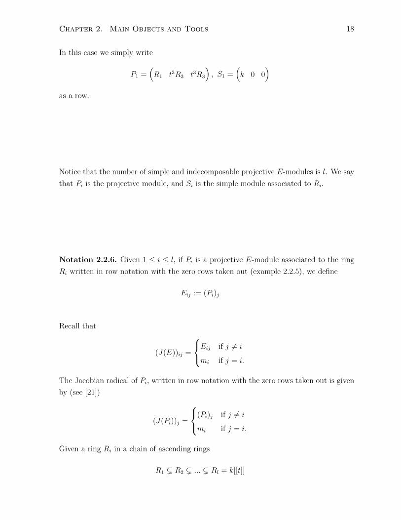
In this case we simply write
P1 =(R1 t3R3 t3R3
), S1 =
(k 0 0
)as a row.
Notice that the number of simple and indecomposable projective E-modules is l. We say
that Pi is the projective module, and Si is the simple module associated to Ri.
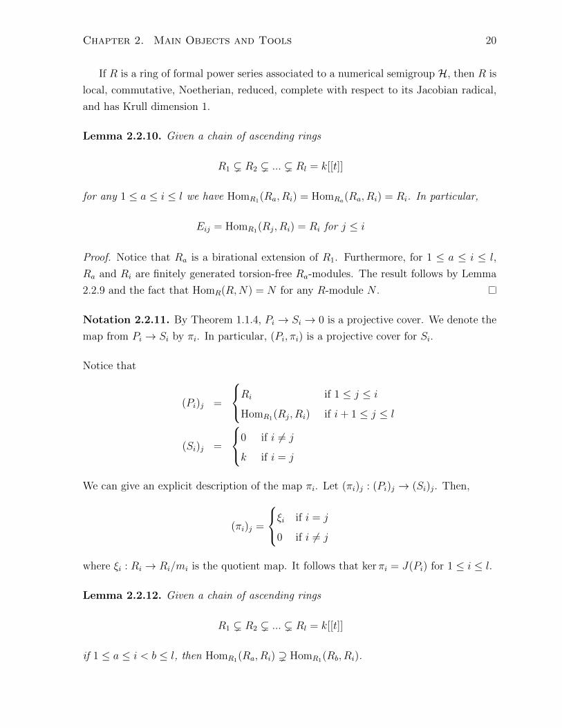
Notation 2.2.6. Given 1 ≤ i ≤ l, if Pi is a projective E-module associated to the ring
Ri written in row notation with the zero rows taken out (example 2.2.5), we define
Eij := (Pi)j
Recall that
(J(E))ij =
Eij if j 6= i
mi if j = i.
The Jacobian radical of Pi, written in row notation with the zero rows taken out is given
by (see [21])
(J(Pi))j =
(Pi)j if j 6= i
mi if j = i.
Given a ring Ri in a chain of ascending rings
R1 ( R2 ( ... ( Rl = k[[t]]

Chapter 2. Main Objects and Tools 19
with Γ(Ri) = {β1, β2, β3, ..., βr} (where β1 < ... < βr = C(Ri)), we define
Ri,0 = Ri = lead{0, β1, β2, ..., βr}
Ri,1 = Ri/k = mi = lead{β1, β2, ..., βr}
Ri,2 = lead{β2, ..., βr}
Ri,3 = lead{β3, ..., βr}
.
.
.
Ri,r = lead{βr} = tC(Ri)Rl
It should be noted that in general, there is no connection between Ri,j and Eij. However,
the notation Ri,j is used extensively in the computation portions of this thesis.
Example 2.2.7. Let R1 = k[[t3, t5, t7]], R2 = k[[t3, t4, t5]], R3 = k[[t]]. Then, C(R1) = 5
and Γ(R1) = {3, 5}. In particular,
R1,0 = R1 = lead{0, 3, 5}
R1,1 = m1 = lead{3, 5}
R1,2 = lead{5} = t5R3
Recall that a finitely generated R-module M is torsion-free provided the natural
map M →M ⊗R R is injective, where R is the total quotient ring of R.
Definition 2.2.8. Suppose R and S are local, Noetherian, commutative, reduced rings,
that are also complete with respect to their Jacobian radicals, respectively, and have
Krull dimension 1. We say that S is a birational extension of R provided R ⊆ S and S
is a finitely generated R-module contained in the total quotient ring R of R.
Notice that if S is a birational extension of R, then every finitely generated torsion-
free S-module is a finitely generated torsion-free R-module, but not vice versa. The
following lemma follows by clearing denominators.
Lemma 2.2.9. Suppose S is a birational extension of R. Let C and D be finitely gen-
erated torsion-free S-modules. Then HomR(C,D) = HomS(C,D). Furthermore, if M is
a finitely generated torsion-free R-module, and f : C →M is an R-linear map, then the
image of f is an S-module.
Chapter 2. Main Objects and Tools 20
If R is a ring of formal power series associated to a numerical semigroup H, then R is
local, commutative, Noetherian, reduced, complete with respect to its Jacobian radical,
and has Krull dimension 1.
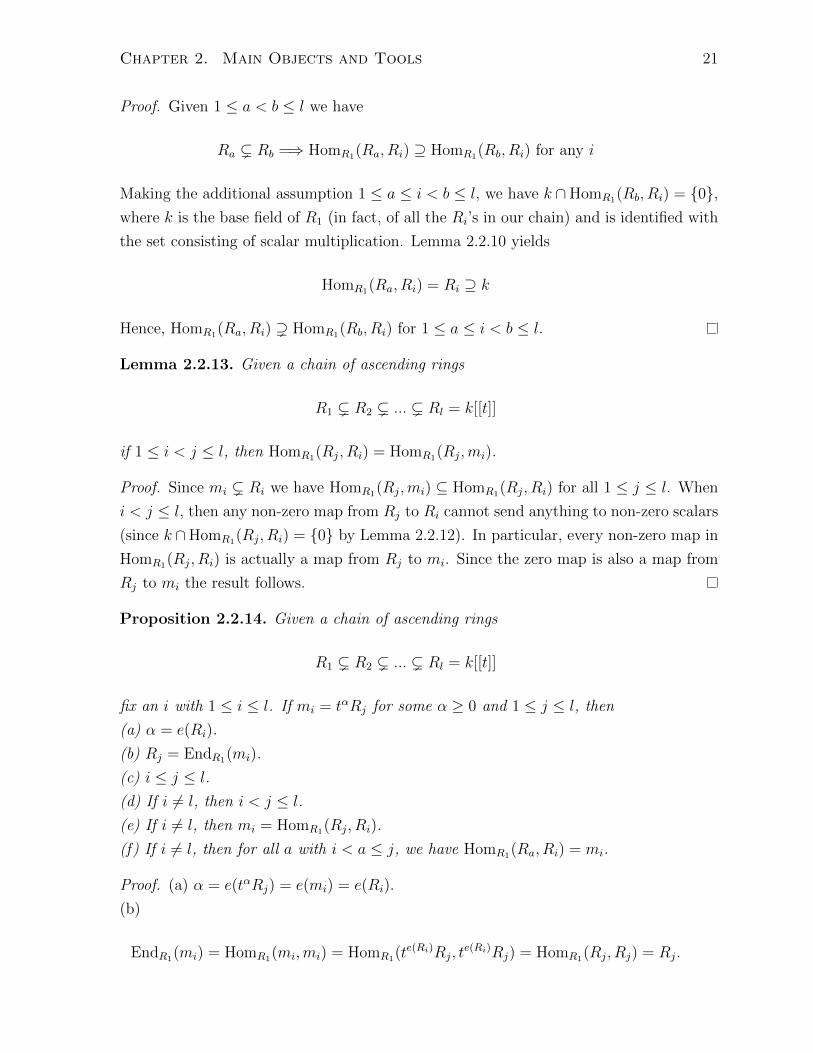
Lemma 2.2.10. Given a chain of ascending rings
R1 ( R2 ( ... ( Rl = k[[t]]
for any 1 ≤ a ≤ i ≤ l we have HomR1(Ra, Ri) = HomRa(Ra, Ri) = Ri. In particular,
Eij = HomR1(Rj, Ri) = Ri for j ≤ i
Proof. Notice that Ra is a birational extension of R1. Furthermore, for 1 ≤ a ≤ i ≤ l,
Ra and Ri are finitely generated torsion-free Ra-modules. The result follows by Lemma
2.2.9 and the fact that HomR(R,N) = N for any R-module N .
Notation 2.2.11. By Theorem 1.1.4, Pi → Si → 0 is a projective cover. We denote the
map from Pi → Si by πi. In particular, (Pi, πi) is a projective cover for Si.
Notice that
(Pi)j =
Ri if 1 ≤ j ≤ i
HomR1(Rj, Ri) if i+ 1 ≤ j ≤ l
(Si)j =
0 if i 6= j
k if i = j
We can give an explicit description of the map πi. Let (πi)j : (Pi)j → (Si)j. Then,
(πi)j =
ξi if i = j
0 if i 6= j
where ξi : Ri → Ri/mi is the quotient map. It follows that ker πi = J(Pi) for 1 ≤ i ≤ l.
Lemma 2.2.12. Given a chain of ascending rings
R1 ( R2 ( ... ( Rl = k[[t]]
if 1 ≤ a ≤ i < b ≤ l, then HomR1(Ra, Ri) ) HomR1(Rb, Ri).
Chapter 2. Main Objects and Tools 21
Proof. Given 1 ≤ a < b ≤ l we have
Ra ( Rb =⇒ HomR1(Ra, Ri) ⊇ HomR1(Rb, Ri) for any i
Making the additional assumption 1 ≤ a ≤ i < b ≤ l, we have k ∩HomR1(Rb, Ri) = {0},where k is the base field of R1 (in fact, of all the Ri’s in our chain) and is identified with
the set consisting of scalar multiplication. Lemma 2.2.10 yields
HomR1(Ra, Ri) = Ri ⊇ k
Hence, HomR1(Ra, Ri) ) HomR1(Rb, Ri) for 1 ≤ a ≤ i < b ≤ l.
Lemma 2.2.13. Given a chain of ascending rings
R1 ( R2 ( ... ( Rl = k[[t]]
if 1 ≤ i < j ≤ l, then HomR1(Rj, Ri) = HomR1(Rj,mi).
Proof. Since mi ( Ri we have HomR1(Rj,mi) ⊆ HomR1(Rj, Ri) for all 1 ≤ j ≤ l. When
i < j ≤ l, then any non-zero map from Rj to Ri cannot send anything to non-zero scalars
(since k ∩HomR1(Rj, Ri) = {0} by Lemma 2.2.12). In particular, every non-zero map in
HomR1(Rj, Ri) is actually a map from Rj to mi. Since the zero map is also a map from
Rj to mi the result follows.
Proposition 2.2.14. Given a chain of ascending rings
R1 ( R2 ( ... ( Rl = k[[t]]
fix an i with 1 ≤ i ≤ l. If mi = tαRj for some α ≥ 0 and 1 ≤ j ≤ l, then
(a) α = e(Ri).
(b) Rj = EndR1(mi).
(c) i ≤ j ≤ l.
(d) If i 6= l, then i < j ≤ l.
(e) If i 6= l, then mi = HomR1(Rj, Ri).
(f) If i 6= l, then for all a with i < a ≤ j, we have HomR1(Ra, Ri) = mi.
Proof. (a) α = e(tαRj) = e(mi) = e(Ri).
(b)
EndR1(mi) = HomR1(mi,mi) = HomR1(te(Ri)Rj, t
e(Ri)Rj) = HomR1(Rj, Rj) = Rj.

Chapter 2. Main Objects and Tools 22
(c) Since Rj = EndR1(mi) ⊇ Ri, we have i ≤ j ≤ l.
(d) If i 6= l, then Rj = EndR1(mi) ) Ri (by construction of the chain), that is i < j ≤ l.
(e) Since i 6= l, part (d) yields i < j ≤ l. By Lemmas 2.2.10 and 2.2.13 we have
HomR1(Rj, Ri) = HomR1(Rj,mi)
= HomR1(Rj, te(Ri)Rj)
= te(Ri) HomR1(Rj, Rj)
= te(Ri)Rj
= mi
(f) If i 6= l, then i < j ≤ l by part (d). For any i < a ≤ j we have Ri ( Ra ⊆ Rj. Lemma
2.2.12 yields
HomR1(Ri, Ri) ) HomR1(Ra, Ri) ⊇ HomR1(Rj, Ri)
In particular, the above chain of inclusions, part (e), and Lemma 2.2.10 yield
mi = HomR1(Rj, Ri) ⊆ HomR1(Ra, Ri) ( HomR1(Ri, Ri) = Ri
Maximality of mi implies that mi = HomR1(Ra, Ri) for all a = i+ 1, . . . , j.
Example 2.2.15. Let
R1 = lead {0, 3, 4, 6}
R2 = EndR1(m1) = lead {0, 3}
R3 = lead {0, 2}
R4 = EndR1(m3) = k[[t]]
Notice that m1 6= t3R2. That is, the converse of part (b) in Proposition 2.2.14 is false.
Lemma 2.2.16. Given an ascending chain of rings
R1 ( R2 ( · · · ( Rl = k[[t]]
then
(a) e(Rl) = C(Rl) = 1, and e(Rl−1) = C(Rl−1).
(b) dimk(Rl/R1) = g(R1)
Chapter 2. Main Objects and Tools 23
Proof. (a) Since Rl = k[[t]] we have e(R1) = 1 = C(R1). Moreover,
Rl = EndR1(ml−1) ⇒ ml−1 = lead {e(Rl−1)}
⇒ Rl−1 = lead {0, e(Rl−1)}
⇒ e(Rl−1) = C(Rl−1)
(b) Let H be the numerical semigroup associated to R1. Suppose b1, b2, ..., br are the
natural numbers missing from H, then Rl/R1 has the set {tbi + R1 : i = 1, 2, . . . , r} as
its basis over k. Hence, dimk(Rl/R1) = g(R1).
Lemma 2.2.17. Let
R1 ( R2 ( ... ( Rl = k[[t]]
be an ascending chain of rings. Then
(a) a1(R1) = e(R1)− 1
(b) 1 ≤ l ≤ g(R1) + 1
(c) e(Ri) = 1⇔ C(Ri) = 0⇔ Ri = k[[t]]⇔ mi = tRi
Proof. (a) a1(R1) = β1 − 1 = e(R1)− 1.
(b) Notice that l = 1 if and only if R1 = k[[t]]. If R1 6= k[[t]], then l ≥ 2. Moreover,
g(R1) is the number of powers of t which are missing from R1, and we atleast put one
power of t in at each stage in our construction, thus, l ≤ g(R1) + 1.
(c) e(Ri) = 1⇔ t ∈ Ri ⇔ C(Ri) = 1⇔ Ri = k[[t]]⇔ mi = tRi = lead {0, 1}.
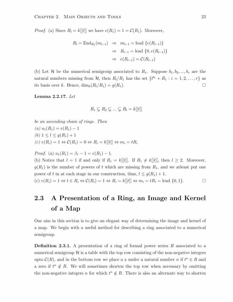
2.3 A Presentation of a Ring, an Image and Kernel
of a Map
Our aim in this section is to give an elegant way of determining the image and kernel of
a map. We begin with a useful method for describing a ring associated to a numerical
semigroup.
Definition 2.3.1. A presentation of a ring of formal power series R associated to a
numerical semigroup H is a table with the top row consisting of the non-negative integers
upto C(R), and in the bottom row we place a x under a natural number n if tn ∈ R and
a zero if tn /∈ R. We will sometimes shorten the top row when necessary by omitting
the non-negative integers n for which tn /∈ R. There is also an alternate way to shorten

Chapter 2. Main Objects and Tools 24
the table and it is as follows: given integers a, b with a ≤ b, we will use the shorthand
notation a . . . b in the top row to mean all the integers between a and b. We put an x in
the second row if those powers are in R and a zero if they are not.
Since every ring of formal power series R associated to a numerical semigroup H is
uniquely determined by Γ(R), each such ring gives rise to a unique presentation and vice
versa.
Example 2.3.2. Let R = k[[t4, t11, t13, t14]]. Then, R has the following presentation:
Powers of t 0 1 2 3 4 5 6 7 8 9 10 11
R x 0 0 0 x 0 0 0 x 0 0 x
The two shorter versions are
Powers of t 0 4 8 11
R x x x x
Powers of t 0 . . . 4 . . . 8 . . . 11
R x 0 x 0 x 0 x
The power of these presentations is that they enable us to find the image and kernel
of maps, as the following example illustrates.
Example 2.3.3. Let
R1 = k[[t4, t11, t13, t14]] = lead {0, 4, 8, 11}
R2 = EndR1(m1) = k[[t4, t7, t9, t10]] = lead {0, 4, 7}
R3 = EndR1(m2) = k[[t3, t4, t5]] = lead {0, 3}
R4 = EndR1(m3) = k[[t]] = lead {0, 1}
Then
E =
R1,0 R1,1 R1,2 R1,3
R2,0 R2,0 R2,1 R2,2
R3,0 R3,0 R3,0 R3,1
R4,0 R4,0 R4,0 R4,0
=
P1
P2
P3
P4
Chapter 2. Main Objects and Tools 25
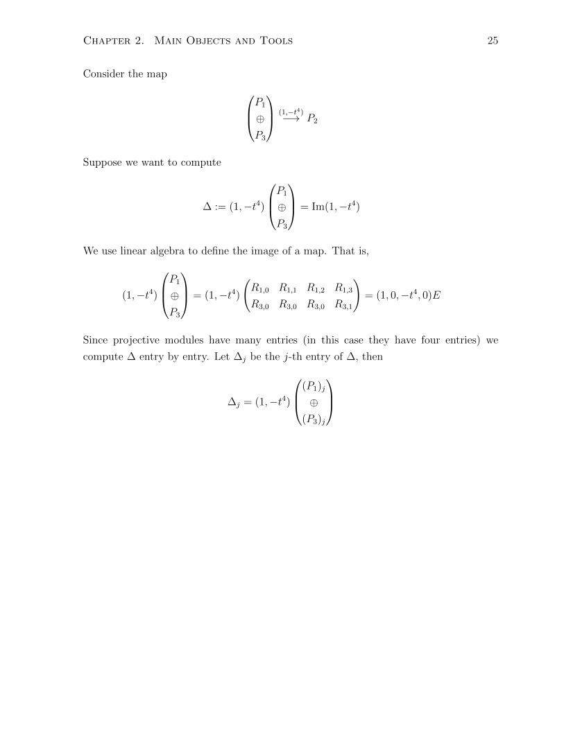
Consider the map P1
⊕P3
(1,−t4)−→ P2
Suppose we want to compute
∆ := (1,−t4)
P1
⊕P3
= Im(1,−t4)
We use linear algebra to define the image of a map. That is,
(1,−t4)
P1
⊕P3
= (1,−t4)
(R1,0 R1,1 R1,2 R1,3
R3,0 R3,0 R3,0 R3,1
)= (1, 0,−t4, 0)E
Since projective modules have many entries (in this case they have four entries) we
compute ∆ entry by entry. Let ∆j be the j-th entry of ∆, then
∆j = (1,−t4)
(P1)j
⊕(P3)j
Chapter 2. Main Objects and Tools 26
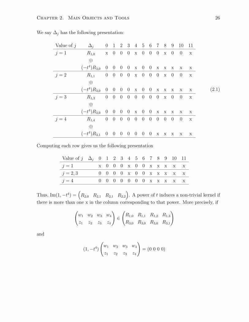
We say ∆j has the following presentation:
Value of j ∆j 0 1 2 3 4 5 6 7 8 9 10 11
j = 1 R1,0 x 0 0 0 x 0 0 0 x 0 0 x
⊕(−t4)R3,0 0 0 0 0 x 0 0 x x x x x
j = 2 R1,1 0 0 0 0 x 0 0 0 x 0 0 x
⊕(−t4)R3,0 0 0 0 0 x 0 0 x x x x x
j = 3 R1,3 0 0 0 0 0 0 0 0 x 0 0 x
⊕(−t4)R3,0 0 0 0 0 x 0 0 x x x x x
j = 4 R1,4 0 0 0 0 0 0 0 0 0 0 0 x
⊕(−t4)R3,1 0 0 0 0 0 0 0 x x x x x
(2.1)
Computing each row gives us the following presentation
Value of j ∆j 0 1 2 3 4 5 6 7 8 9 10 11
j = 1 x 0 0 0 x 0 0 x x x x x
j = 2, 3 0 0 0 0 x 0 0 x x x x x
j = 4 0 0 0 0 0 0 0 x x x x x
Thus, Im(1,−t4) =(R2,0 R2,1 R2,1 R2,2
). A power of t induces a non-trivial kernel if
there is more than one x in the column corresponding to that power. More precisely, if(w1 w2 w3 w4
z1 z2 z3 z4
)∈
(R1,0 R1,1 R1,2 R1,3
R3,0 R3,0 R3,0 R3,1
)
and
(1,−t4)
(w1 w2 w3 w4
z1 z2 z3 z4
)= (0 0 0 0)

Chapter 2. Main Objects and Tools 27
then wi − t4zi = 0 for i = 1, 2, 3, 4. This can be given the following presentation:
Value of j 0 1 2 3 4 5 6 7 8 9 10 11 12
j = 1 0 0 0 0 x11 0 0 0 x1
2 0 0 x13 x1
4 ⊆ R1,0
x11 0 0 0 x1
2 0 0 x13 x1
4 x15 x1
6 x17 x1
8 ⊆ R3,0
j = 2 0 0 0 0 x21 0 0 0 x2
2 0 0 x23 x2
4 ⊆ R1,1
x21 0 0 0 x2
2 0 0 x23 x2
4 x25 x2
6 x27 x2
8 ⊆ R3,0
j = 3 0 0 0 0 0 0 0 0 x31 0 0 x3
2 x33 ⊆ R1,2
0 0 0 0 x31 0 0 x3
2 x33 x3
4 x35 x3
6 x37 ⊆ R3,0
j = 4 0 0 0 0 0 0 0 0 0 0 0 x41 x4
2 ⊆ R1,3
0 0 0 0 0 0 0 x41 x4
2 x43 x4
4 x45 x4
6 ⊆ R3,1
(2.2)
Where x11 says the coefficient of t4 in (P1)1 = R1,0 must equal the scalar in (P3)1 = R3,0.
Similar idea works for the other xji . As one can see, notationally this becomes very messy,
as such we abuse notation and simply give the following presentation for the ker(1,−t4):
Value of j 0 1 2 3 4 5 6 7 8 9 10 11
j = 1 0 0 0 0 x 0 0 0 x 0 0 x
x 0 0 0 x 0 0 x x x x x
j = 2 0 0 0 0 x 0 0 0 x 0 0 x
x 0 0 0 x 0 0 x x x x x
j = 3 0 0 0 0 0 0 0 0 x 0 0 x
0 0 0 0 x 0 0 x x x x x
j = 4 0 0 0 0 0 0 0 0 0 0 0 x
0 0 0 0 0 0 0 x x x x x
(2.3)
Since the presentation for j = 1 and j = 2 are the same we shorten the presentation as
follows:
Value of j 0 1 2 3 4 5 6 7 8 9 10 11
j = 1, 2 0 0 0 0 x 0 0 0 x 0 0 x
x 0 0 0 x 0 0 x x x x x
j = 3 0 0 0 0 0 0 0 0 x 0 0 x
0 0 0 0 x 0 0 x x x x x
j = 4 0 0 0 0 0 0 0 0 0 0 0 x
0 0 0 0 0 0 0 x x x x x
(2.4)

Chapter 2. Main Objects and Tools 28
It thus follows that
ker(1,−t4) =
(t4y1 t4y2 t4y3 t4y4
y1 y2 y3 y4
)
where y1, y2 ∈ R2,0, y3 ∈ R2,1, y4 ∈ R2,2. In particular,
ker(1,−t4) =
(t4
1
)P2
The presentation in (2.4) can be obtained much quicker if we look at the original presen-
tation in (2.1) and reverse the action of (1,−t4) on each row on the columns that have
more than one x in them. For example,
Value of j ∆j 0 1 2 3 4 5 6 7 8 9 10 11
j = 1 R1,0 x 0 0 0 x 0 0 0 x 0 0 x
⊕(−t4)R3,0 0 0 0 0 x 0 0 x x x x x
Notice that columns 4, 8, and 11 and on have more than one x appearing in them. The
action of (1,−t4) on the first row is multiplication by 1, the reverse of this process is
to leave things as they are in the columns with more than one x. However, the action
of (1,−t4) on the second row is multiplication by −t4, the reverse of this action is to
decrease the powers by 4 in the columns with more than one x. Which gives the following
presentation;
Value of j 0 1 2 3 4 5 6 7 8 9 10 11
j = 1 0 0 0 0 x 0 0 0 x 0 0 x
x 0 0 0 x 0 0 x x x x x
Same as the result in (2.3). The same idea works for other maps, however, the more
columns and rows in the map, the more relations that the kernel will have (the xji ’s that
appear in (2.2)).
Remark 2.3.4. Suppose Af−→ B, where f can be expressed as a row matrix. Then the
preceding discussion shows that f is injective if and only if in the presentation of image
of f every column has at most one x in it.
Chapter 2. Main Objects and Tools 29
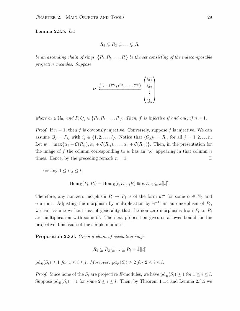
Lemma 2.3.5. Let
R1 ( R2 ( . . . ( Rl
be an ascending chain of rings, {P1, P2, . . . , Pl} be the set consisting of the indecomposable
projective modules. Suppose
P
Q1
Q2
...
Qn
f := (ta1 , ta2 , . . . , tan)
where ai ∈ N0, and P,Qj ∈ {P1, P2, . . . , Pl}. Then, f is injective if and only if n = 1.
Proof. If n = 1, then f is obviously injective. Conversely, suppose f is injective. We can
assume Qj = Pij with ij ∈ {1, 2, . . . , l}. Notice that (Qj)1 = Rij for all j = 1, 2, . . . n.
Let w = max{α1 + C(Ri1), α2 + C(Ri2), . . . , αn + C(Rin)}. Then, in the presentation for
the image of f the column corresponding to w has an “x” appearing in that column n
times. Hence, by the preceding remark n = 1.
For any 1 ≤ i, j ≤ l,
HomE(Pi, Pj) = HomE(eiE, ejE) ∼= ejEei ⊆ k[[t]].
Therefore, any non-zero morphism Pi → Pj is of the form utα for some α ∈ N0 and
u a unit. Adjusting the morphism by multiplication by u−1, an automorphism of Pj,
we can assume without loss of generality that the non-zero morphisms from Pi to Pj
are multiplication with some tα. The next proposition gives us a lower bound for the
projective dimension of the simple modules.
Proposition 2.3.6. Given a chain of ascending rings
R1 ( R2 ( ... ( Rl = k[[t]]
pdE(Si) ≥ 1 for 1 ≤ i ≤ l. Moreover, pdE(Si) ≥ 2 for 2 ≤ i ≤ l.
Proof. Since none of the Si are projective E-modules, we have pdE(Si) ≥ 1 for 1 ≤ i ≤ l.
Suppose pdE(Si) = 1 for some 2 ≤ i ≤ l. Then, by Theorem 1.1.4 and Lemma 2.3.5 we

Chapter 2. Main Objects and Tools 30
have the following exact sequence for some α ≥ 0, 1 ≤ j ≤ l;
0 Si Pi Pj 0πi tα
(2.5)
The entries of Si are zero except for the i-th entry which is k. Since i 6= 1, (2.5) yields
the following exact sequence;
0 (Si)1 = 0 (Pi)1 = Ri (Pj)1 = Rj 0(πi)1 tα
In particular, tαRj = Ri, this implies that α = 0 (since k is a subset of Ri) which in turn
yields i = j. Furthermore, since the i-th entry of Si is k and the i-th entry of Pi is Ri,
(2.5) gives us the following exact sequence;
0 k = Ri/mi Ri Ri 0id
That is, mi = Ri, a contradiction. Hence, pdE(Si) ≥ 2 for 2 ≤ i ≤ l, completing the
proof.
The next proposition gives a necessary and sufficient condition for pdE(S1) = 1.
Proposition 2.3.7. Given a chain of ascending rings
R1 ( R2 ( ... ( Rl = k[[t]]
pdE(S1) = 1 if and only if m1 = te(R1)Rj for some 1 < j ≤ l.
Proof. Suppose pdE(S1) = 1, then, by Theorem 1.1.4 and Lemma 2.3.5 we have the
following exact sequence for some α ≥ 0, 1 ≤ j ≤ l;
0 S1 P1 Pj 0π1 tα
Therefore,
0 k = R1/m1 R1 Rj 0ξ tα

Chapter 2. Main Objects and Tools 31
is a short exact sequence, where ξ is the quotient map. Therefore, m1 = tαRj where,
α = e(R1), 1 < j ≤ l (Proposition 2.2.14).
Conversely, suppose m1 = te(R1)Rj for some 1 < j ≤ l. Then, for 2 ≤ a ≤ j we have
R1 ( Ra ⊆ Rj and Lemma 2.2.12 implies that
R1 = HomR1(R1, R1) ) HomR1(Ra, R1) ⊇ HomR1(Rj, R1)
Since m1 ( R1 we have
HomR1(Ra,m1) ⊆ HomR1(Ra, R1)
In particular,
R1 = HomR1(R1, R1) ) HomR1(Ra, R1)
= HomR1(Ra,m1) (Lemma 2.2.13)
= HomR1(Ra, te(R1)Rj)
= te(R1) HomR1(Ra, Rj)
= te(R1)Rj (Lemma 2.2.10)
= m1
Maximality of m1 implies that m1 = HomR1(Ra, R1) = HomR1(Ra,m1). Moreover, for
j + 1 ≤ a ≤ l, using Proposition 2.2.13 yields
HomR1(Ra, R1) = HomR1(Ra,m1) = HomR1(Ra, te(R1)Rj) = te(R1) HomR1(Ra, Rj)
It follows that
(P1)a =
R1 if a = 1
m1 if 2 ≤ a ≤ j
HomR1(Ra, R1) if j + 1 ≤ a ≤ l
=
R1 if a = 1
te(R1)Rj if 2 ≤ a ≤ j
te(R1) HomR1(Ra, Rj) if j + 1 ≤ a ≤ l

Chapter 2. Main Objects and Tools 32
and
(Pj)a = Eja =
Rj if 1 ≤ a ≤ j
HomR1(Ra, Rj) if j + 1 ≤ a ≤ l
That is,
0 S1 P1 Pj 0π1 te(R1)
is a projective resolution for S1, and it is minimal by Proposition 2.3.6, completing the
proof.
In example 2.2.15, m2 = t3R4 , however, pdE(S2) ≥ 2 by Proposition 2.3.6. In
particular, Proposition 2.3.7 fails to hold if we replace S1 by Si for some 1 < i ≤ l.
2.4 Structure of E
We now turn our attention to the entries of the matrix E and how the entries in a given
row are related to the entries in the rows preceding it and succeeding it.
Lemma 2.4.1. Let
R1 ( R2 ( ... ( Rl = k[[t]]
be an ascending chain of rings. The entries of the matrix E satisfy the following proper-
ties;
(a) If 1 ≤ j ≤ i ≤ l,, then Eij = Ri.
(b) Eij ⊇ Ei(j+1) (that is, there is a descending chain of rings or modules as we go across
a given row. Note that Eij could equal Ei(j+1), for example, E21 = E22 = R2 always).
Furthermore, Eij ⊆ E(i+1)j (there is an ascending chain of rings or modules as we go
down a given column).
(c) If 1 ≤ i ≤ l − 1, then Eii ) Ei(i+1).
(d) HomR1(EndR1(ml), Rl) = Rl. If i 6= l, then HomR1(EndR1(mi), Ri) = mi.
(e) If 1 ≤ i ≤ l − 1, then Ei(i+1) = mi.
(f) Eil = tC(Ri)Rl for 1 ≤ i ≤ l − 1 and Ell = Rl
Proof. (a) This follows from Lemma 2.2.10.
(b) This follows from the fact that HomR1(�, Ri) is a contravariant functor and HomR1(Ri,�)
is a covariant functor.

Chapter 2. Main Objects and Tools 33
(c) This is a consequence of part (b) and Lemma 2.2.12.
(d) The first part follows from part (a) and the fact that EndR1(ml) = Rl. If i 6= l then
by Theorem 1.1.1, Ri ( EndR1(mi). That is, k ∩ HomR1(EndR1(mi), Ri) = {0} (where
k is the base field of R1, in fact, of all the Ri, and it is identified with scalar multiplica-
tion) and Ri = HomR1(Ri, Ri) ) HomR1(EndR1(mi), Ri). Given a non-negative integer
b, tb ∈ EndR1(mi) if and only if tbtx = tb+x ∈ mi for any tx ∈ mi, in particular,
HomR1(EndR1(mi), Ri) ⊇ mi.
Thus,
Ri ) HomR1(EndR1(mi), Ri) ⊇ mi,
the maximality of mi gives the desired result.
(e) Given 1 ≤ i ≤ l − 1, we have Ri ( Ri+1 ⊆ EndR1(mi). Parts (a), (c) and (d) imply
that
Ri = Eii ) Ei(i+1) ⊇ HomR1(EndR1(mi), Ri) = mi.
Maximality of mi gives Ei(i+1) = mi.
(f) Given 1 ≤ i ≤ l − 1, since Rl = k[[t]]
Eil = HomR1(Rl, Ri) = tC(Ri)Rl
The second part follows form part (a).
The preceding proposition gives us a very nice description of the entries of E on its
main diagonal, below it, the entries right above the main diagonal (Ei(i+1)), and the
entries in column l. In particular,
E =
R1 m1 ∗ ∗ ∗ ∗ ∗ ∗ tC(R1)Rl
R2 R2 m2 ∗ ∗ ∗ ∗ ∗ tC(R2)Rl
R3 R3 R3 m3 ∗ ∗ ∗ ∗ tC(R3)Rl
R4 R4 R4 R4 m4 ∗ ∗ ∗ tC(R4)Rl
......
......
. . . . . . ∗ ∗ ...
Rl−1 Rl−1 Rl−1 Rl−1 . . . tC(Rl−1)Rl
Rl Rl Rl Rl . . . Rl

Chapter 2. Main Objects and Tools 34
The ∗ entries are unknown and must be computed on a base by base cases. Notice that
ml−1 = tC(Rl−1)Rl by Lemma 2.2.16(a). We conclude this section by looking at the entries
of E when the ring R has the property e(R) = C(R).
Lemma 2.4.2. Let
R1 ( R2 ( ... ( Rl = k[[t]]
be an ascending chain of rings, and suppose e(Ri) = C(Ri) for some 1 ≤ i ≤ l. Then
Eij =
Ri if 1 ≤ j ≤ i
te(Ri)Rl if i+ 1 ≤ j ≤ l
Proof. By Proposition 2.4.1 Eij = Ri for 1 ≤ j ≤ i. Moreover, e(Ri) = C(Ri) implies
that
Ri = lead {0, e(Ri)}
Then, for any j with i+ 1 ≤ j ≤ l
HomR1(Rj, Ri) = lead {e(Ri)} = te(Ri)Rl
Proposition 2.4.3. Let
R1 ( R2 ( ... ( Rl = k[[t]]
be an ascending chain of rings. Then, pdE(Sl) = 2.
Proof. By Lemma 2.2.16(a) we have Rl−1 = lead {e(Rl−1)} with e(Rl−1) = C(Rl−1). By
Lemma 2.4.2
E(l−1)j =
Ri if 1 ≤ j ≤ l − 1
te(Rl−1)Rl if j = l
Let
∆ = (1, t)
Pl−1⊕Pl
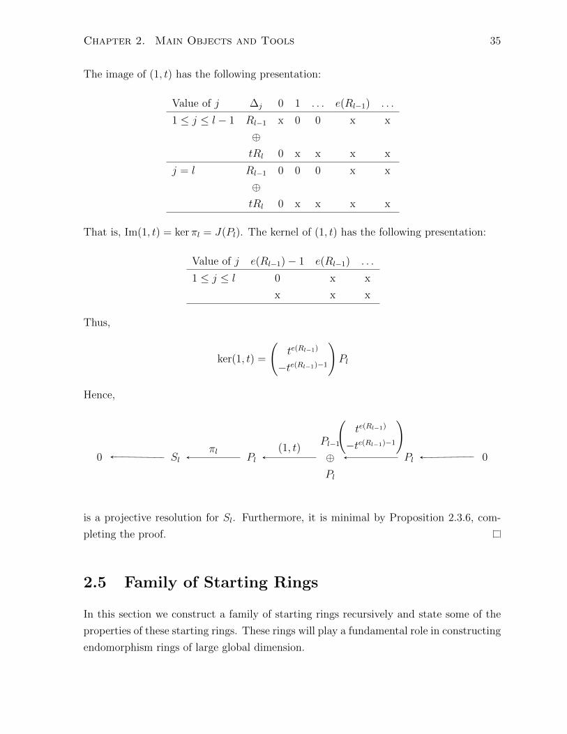
Chapter 2. Main Objects and Tools 35
The image of (1, t) has the following presentation:
Value of j ∆j 0 1 . . . e(Rl−1) . . .
1 ≤ j ≤ l − 1 Rl−1 x 0 0 x x
⊕tRl 0 x x x x
j = l Rl−1 0 0 0 x x
⊕tRl 0 x x x x
That is, Im(1, t) = ker πl = J(Pl). The kernel of (1, t) has the following presentation:
Value of j e(Rl−1)− 1 e(Rl−1) . . .
1 ≤ j ≤ l 0 x x
x x x
Thus,
ker(1, t) =
(te(Rl−1)
−te(Rl−1)−1
)Pl
Hence,
0 Sl Pl
Pl−1
⊕Pl
Pl 0πl (1, t)
(te(Rl−1)
−te(Rl−1)−1
)
is a projective resolution for Sl. Furthermore, it is minimal by Proposition 2.3.6, com-
pleting the proof.
2.5 Family of Starting Rings
In this section we construct a family of starting rings recursively and state some of the
properties of these starting rings. These rings will play a fundamental role in constructing
endomorphism rings of large global dimension.
Chapter 2. Main Objects and Tools 36
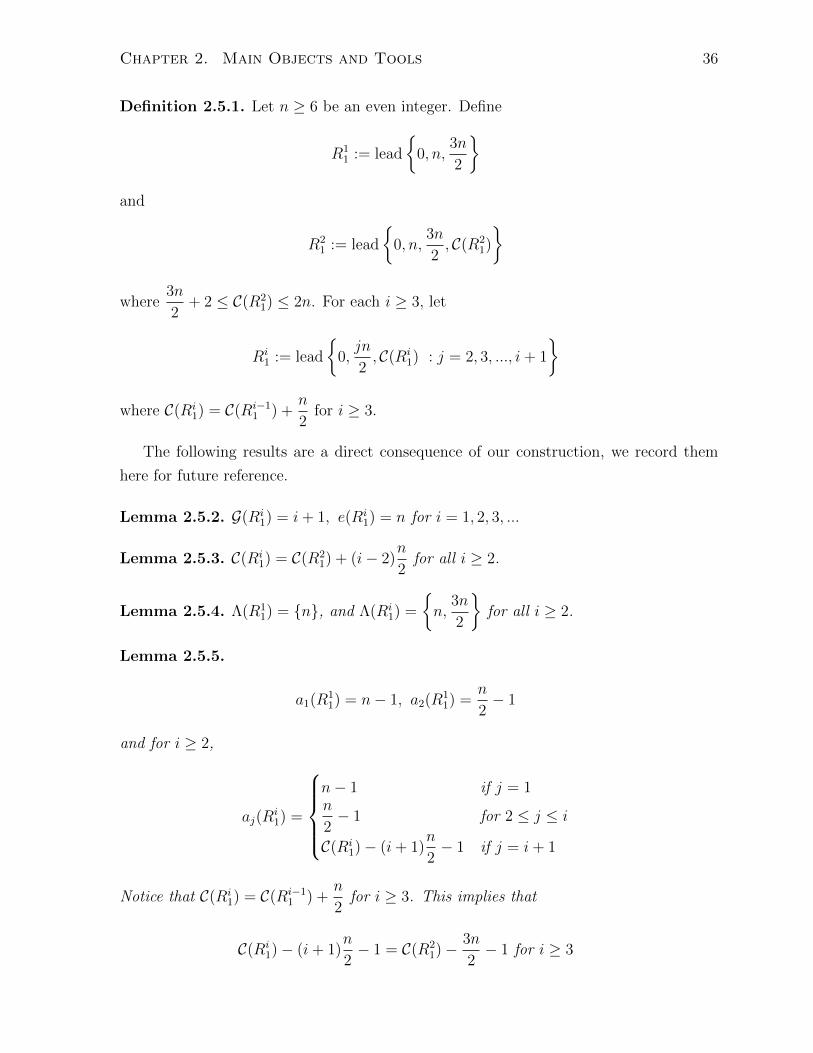
Definition 2.5.1. Let n ≥ 6 be an even integer. Define
R11 := lead
{0, n,
3n
2
}and
R21 := lead
{0, n,
3n
2, C(R2
1)
}
where3n
2+ 2 ≤ C(R2
1) ≤ 2n. For each i ≥ 3, let
Ri1 := lead
{0,jn
2, C(Ri
1) : j = 2, 3, ..., i+ 1
}
where C(Ri1) = C(Ri−1
1 ) +n
2for i ≥ 3.
The following results are a direct consequence of our construction, we record them
here for future reference.
Lemma 2.5.2. G(Ri1) = i+ 1, e(Ri
1) = n for i = 1, 2, 3, ...
Lemma 2.5.3. C(Ri1) = C(R2
1) + (i− 2)n
2for all i ≥ 2.
Lemma 2.5.4. Λ(R11) = {n}, and Λ(Ri
1) =
{n,
3n
2
}for all i ≥ 2.
Lemma 2.5.5.
a1(R11) = n− 1, a2(R
11) =
n
2− 1
and for i ≥ 2,
aj(Ri1) =
n− 1 if j = 1n
2− 1 for 2 ≤ j ≤ i
C(Ri1)− (i+ 1)
n
2− 1 if j = i+ 1
Notice that C(Ri1) = C(Ri−1
1 ) +n
2for i ≥ 3. This implies that
C(Ri1)− (i+ 1)
n
2− 1 = C(R2
1)−3n
2− 1 for i ≥ 3

Chapter 2. Main Objects and Tools 37
Notice the above equality is also true when i = 2. Hence, for i ≥ 2 we have
aj(Ri1) =
n− 1 if j = 1n
2− 1 for 2 ≤ j ≤ i
C(R21)−
3n
2− 1 if j = i+ 1
Lemma 2.5.6. Γ(R11) =
{n,
3n
2
}, and for i ≥ 2 we have Γ(Ri
1) ={βi1, β
i2, ..., β
ii+1
}where
βij =
n+ (j − 1)n
2if 1 ≤ j ≤ i
C(Ri1) if j = i+ 1
Definition 2.5.7. Suppose
R1 ( R2 ( . . . ( Rl = k[[t]]
is a chain of ascending rings. Fix i, and suppose Γ(Ri) = {β1, β2, ..., βr} with β1 < β2 <
... < βr = C(Ri). Let γ1 be the number of positive powers of t between tC(Ri)−β1 and
tC(Ri) (inclusive) which are missing from Ri. Let γ2 be the number of positive powers of
t between tC(Ri)−β2 and tC(Ri)−β1−1 (inclusive) which are missing from Ri, continuing this
process, this stops at γr, the number of positive powers of t between tC(Ri)−βr = t0 and
tC(Ri)−βr−1−1 (inclusive) which are missing from Ri. Define
Φ(Ri) = {γj | j = 1, 2, ..., r}
Lemma 2.5.8. Φ(R11) = {γ11 , γ12} =
{n− 1,
n
2− 1}
, and for i ≥ 2 we have Φ(Ri1) ={
γi1, γi2, ..., γ
ii+1
}where
γij =
n− 2 if j = 1n
2− 1 if 2 ≤ j ≤ i− 1
n
2if j = i
C(Ri1)− βii − 1 if j = i+ 1
Notice that
C(Ri1)− βii − 1 = C(R2
1) + (i− 2)n
2−(n+ (i− 1)
n
2
)− 1 = C(R2
1)−3n
2− 1

Chapter 2. Main Objects and Tools 38
That is, for i ≥ 2 we have
γij =
n− 2 if j = 1n
2− 1 if 2 ≤ j ≤ i− 1
n
2if j = i
C(R21)−
3n
2− 1 if j = i+ 1
Suppose
R1 ( R2 ( . . . ( Rl = k[[t]]
is a chain of ascending rings. Given 1 ≤ i ≤ l, if e(Ri) < C(Ri) then Λ(Ri) is not empty.
Let
Λ(Ri) = {α1, ..., αs}, Γ(Ri) = {β1, ..., βr},
where the elements are listed in ascending order. Since Λ(Ri) ⊆ Γ(Ri), for each αa ∈Λ(Ri) there exists a βja ∈ Γ(Ri) such that αa = βja . Since α1 = β1 we have a = 1 = j1.
However, for a ≥ 2 this need not be the case. This leads us to the following useful
definition.
Definition 2.5.9. Given 1 ≤ i ≤ l, let
Λ(Ri) = {α1, ..., αs}
Γ(Ri) = {β1, ..., βr}
Φ(Ri) = {γ1, ..., γr}
For each a ∈ {1, 2, ..., s}, define
λa = i+
ja∑h=1
γh
Since j1 = 1 we have λ1 = i+ γ1. We define
χ(Ri) = {λ1, ..., λs}
If e(Ri) = C(Ri), we define χ(Ri) = ∅. If follows that |χ(Ri)| = |Λ(Ri)|.

Chapter 2. Main Objects and Tools 39
Example 2.5.10. Let R1 = k[[t5, t11, t14, t17, t18]], then
C(R1) = 14
Λ(R1) = {5, 11}
Γ(R1) = {5, 10, 11, 14}
Φ(R1) = {γ1, γ2, γ3, γ4} = {3, 4, 1, 2}
Using the notation above we have α1 = 5 = β1, α2 = β3, that is, a = 1 = j1 and j2 = 3.
Moreover,
λ1 = 1 + γ1 = 4
λ2 = 1 +3∑
h=1
γh = 1 + 3 + 4 + 1 = 9
which yields χ(R1) = {4, 9}.
Lemma 2.5.11. χ(R11) = {λ11} = {γ11 + 1} = {(n− 1) + 1 = n}, and for i ≥ 2 we have
χ(Ri1) = {λi1, λi2} where
λij =
1 + γi1 = n− 1 if j = 1
1 + γi1 + γi2 if j = 2
Moreover,
λ2j =
1 + γ21 = n− 1 if j = 1
1 + γ21 + γ22 =3n
2− 1 if j = 2
and for i ≥ 3
λij =
1 + γi1 = n− 1 if j = 1
1 + γi1 + γi2 =3n
2− 2 if j = 2
2.6 The symbol d e
In this section we focus on the symbol d e and its properties.
Definition 2.6.1. Let X be a 1 × l row matrix, and Xj be its j-th entry. Given an

Chapter 2. Main Objects and Tools 40
integer a ≥ 0, we define Xdae to be a 1× (l + a) row matrix with the following entries:
(Xdae)j =
X1 if 1 ≤ j ≤ a
Xj−a if a+ 1 ≤ j ≤ l + a
That is, we are putting a string of X1’s (in fact, a of them) at the beginning of X to
obtain Xdae. Notice that
Xd0e = X
Given integers a, b ≥ 0,
(Xdae)dbe = Xda+ be = (Xdbe)dae
Notation 2.6.2. Let p ∈ N, and X i be a 1× l row matrix for i = 1, 2, ..., p. We define
X =
p⊕i=1
X i =
X1
X2
...
Xp
It follows that X is a p× l matrix.
Definition 2.6.3. Given
X =
p⊕i=1
X i
where X i are 1× l row matrices, we define
Xdae =
p⊕i=1
X idae =
X1daeX2dae
...
Xpdae
Given an integer a ≥ 0, if f : X → Y is a map given in matrix form, where
X =
p⊕i=1
X i, Y =
p⊕i=1
Y i

Chapter 2. Main Objects and Tools 41
and X i, Y i are 1 × l row matrices, then f has p columns. Since the number of rows of
Xdae, Y dae is also p, we define fdae : Xdae → Y dae by setting fdae = f (the only thing
we have done is change the domain and co-domain). We abuse notation and we use f in
place of fdae.
Let
R1 ( R2 ( R3 ( ... ( Rl−1 ( Rl = k[[t]]
be an ascending chain constructed in section 2.2. The maps πi : Pi → Si are not given
by a matrix . We define
πidae : Pidae → Sidae
as follows;
(π1dae)j =
ξi if 1 ≤ j ≤ a+ 1
0 if a+ 2 ≤ j ≤ l + a
and for 2 ≤ i ≤ l,
(πidae)j =
ξi if j = i+ a
0 if j 6= i+ a
where ξi : Ri → Ri/mi is the quotient map, Pi, Si are 1× l row matrices, and
(S1dae)j =
k if 1 ≤ j ≤ a+ 1
0 if a+ 2 ≤ j ≤ l + a
(P1dae)j =
R1 if 1 ≤ j ≤ a+ 1
(P1)j−a if a+ 2 ≤ j ≤ l + a,
for 2 ≤ i ≤ l,
(Sidae)j =
k if j = i+ a
0 if j 6= i+ a
(Pidae)j =
Ri if 1 ≤ j ≤ a+ 1
(Pi)j−a if a+ 2 ≤ j ≤ l + a

Chapter 2. Main Objects and Tools 42
Example 2.6.4. Suppose R1 = k[[t3, t4, t5]], R2 = k[[t2, t3]], R3 = k[[t]]. Then
E =
R1 t3R3 t3R3
R2 R2 t2R3
R3 R3 R3
and
S1d2e =(k k k 0 0
)S2d2e =
(0 0 0 k 0
)P1d2e =
(R1 R1 R1 t3R3 t3R3
)= (P1d1e)d1e
P2d2e =(R2 R2 R2 R2 t2R3)
)P1
⊕P2
d2e =
(P1d2eP2d2e
)=
(R1 R1 R1 t3R3 t3R3
R2 R2 R2 R2 t2R3
)=
P1d2e⊕
P2d2e
Moreover,
π1d2e : P1d2e → S1d2e and (π1d2e)j =
ξ1 if 1 ≤ j ≤ 3
0 if 4 ≤ j ≤ 5
π2d2e : P2d2e → S2d2e and (π2d2e)j =
ξ2 if j = 4
0 if j 6= 4
The following two results are an immediate consequence of our definitions above and
we record them here for future reference.
Lemma 2.6.5. Let p ∈ N. Suppose
X =
p⊕i=1
X i, Y =
p⊕i=1
Y i, Z =
p⊕i=1
Zi
where X i, Y i, Zi are 1× l rows. If
Xdae f→ Y dae g→ Zdae

Chapter 2. Main Objects and Tools 43
is exact at Y dae (i.e. ker g = Im(f)) for some a ∈ N0, then
Xdbe f→ Y dbe g→ Zdbe
is exact at Y dbe for every b ∈ N0.
Lemma 2.6.6. Using the notation in Proposition 2.6.5,
Im(X
f→ Y)⊆ J(Y )
if and only if
Im(Xdae f−→ Y dae
)⊆ J(Y dae) for any a ∈ N0
Chapter 3
“Lazy” Construction
In this chapter we concentrate on a construction of our chain which maximizes its length,
called the “lazy” construction. More specifically, in section 3.1 we give the precise defi-
nition of this construction and introduce some of the necessary notation. In section 3.2
we compute the global dimension of endomorphism rings for specific starting rings. In
Section 3.3 we give some of the results which are a consequence of this construction.
Section 3.4 focuses on computing the global dimension of endomorphism rings when the
length of the chain is small. In section 3.5 we combine this construction with the family
of starting rings constructed in section 2.5 to obtain a set of endomorphism rings whose
global dimensions are arbitrarily large (but finite).
3.1 The Construction
Given a numerical semigroup H, let R be the ring of formal power series associated to
H. Then, H has a minimal generating set, say {α1, α2, ..., αs} written in ascending order.
That is,
H = 〈α1, α2, ..., αs〉 ⇔ R = k[[tα1 , tα2 , ..., tαs ]]
Given a non-negative integer b with b 6= αi, we define
H[[b]] = 〈α1, α2, ..., αs, b〉
Since gcd(α1, α2, ..., αs) = 1 implies that gcd(α1, α2, ..., αs, b) = 1, the set H[[b]] is a
numerical semigroup. We define R[[tb]] to be the ring of formal power series associated
to H[[b]]. It should be noted that H ⊆ H[[b]], and equality holds if and only if b ∈ H.
44

Chapter 3. “Lazy” Construction 45
We are now in position to describe the “lazy” construction.
Let H be a numerical semigroup with minimal generating set {α1, α2, ..., αs}, and
F (α1, α2, ..., αs) ≥ 1 (i.e. 1 /∈ H). Let R1 be the ring of formal power series associated
to H. We define
Ri = Ri−1[[tC(Ri−1)−1]] for i ≥ 2
Since only finitely many powers of t are missing from R1, there exists an l ≥ 2 such that
Rl = k[[t]]. In particular, we have constructed the following ascending chain of rings:
R1 ( R2 ( · · · ( Rl = k[[t]] (3.1)
Let
M :=
(l⊕
i=1
Ri
), E := EndR1(M)
We say the ascending chain in (3.1), M , and E are constructed via the “lazy” construc-
tion.
For 1 ≤ i ≤ l − 1 we have Ri 6= k[[t]]. Lemma 2.1.3(e) yields tC(Ri)−1 /∈ Ri and
tx ∈ Ri for all x ≥ C(Ri). In particular, Ri ( Ri+1 ⊆ EndR1(mi). Hence, gl. dim(E) ≤ l
(Proposition 2.2.2).
Lemma 3.1.1. Let
R1 ( R2 ( ... ( Rl
be an ascending chain of ring constructed via the ”lazy” construction. Then,
(a) 1 ≤ l = g(R1) + 1, e(Rl) = C(Rl) = 1. If l ≥ 2, then e(Rl−1) = C(Rl−1) = 2.
(b) e(Ri) ≤ e(Ri−1) for i = 2, 3, ..., l. Moreover, if e(Ri−1) = C(Ri−1) then e(Ri) =
e(Ri−1)− 1.
(c) C(Ri) ≤ C(Ri−1)− 1 for i = 2, 3, ..., l. Moreover, if e(Ri−1) = C(Ri−1), then C(Ri) =
C(Ri−1)− 1.
(d) If e(Ri) = C(Ri) for some i = 1, 2, ..., l, then e(Rj) = C(Rj) for all i ≤ j ≤ l.
Proof. (a) Notice that l = 1⇔ R1 = k[[t]]. If R1 6= k[[t]], then l ≥ 2. Since g(R1) is the
number of powers of t which are missing from R1 and we put them in one at a time to
construct our chain, we have l = g(R1) + 1. Also, Rl = k[[t]] ⇒ e(Rl) = C(Rl) = 1. If
l ≥ 2, then Rl−1 = k[[t2, t3]]⇒ e(Rl−1) = C(Rl−1) = 2.
Chapter 3. “Lazy” Construction 46
(b) Since Ri−1 ( Ri we have e(Ri) ≤ e(Ri−1). If e(Ri−1) = C(Ri−1), then Ri−1 =
lead {0, e(Ri−1)} ⇒ Ri = lead {0, e(Ri−1)− 1} ⇒ e(Ri) = e(Ri−1)− 1.
(c) Since Ri−1 ( Ri we have C(Ri) ≤ C(Ri−1) − 1. If e(Ri−1) = C(Ri−1), then Ri−1 =
lead {0, C(Ri−1)} ⇒ Ri = lead {0, C(Ri−1)− 1} ⇒ C(Ri) = C(Ri−1)− 1.
(d) By part (b) e(Ri+1) = e(Ri)− 1, and by part (c) C(Ri+1) = C(Ri)− 1. In particular,
e(Ri+1) = e(Ri)− 1 = C(Ri)− 1 = C(Ri+1). A similar proof shows the result is true for
i+ 2, i+ 3, ..., l.
The projective modules under the lazy construction have a very nice description. We
state this as a lemma for future reference.
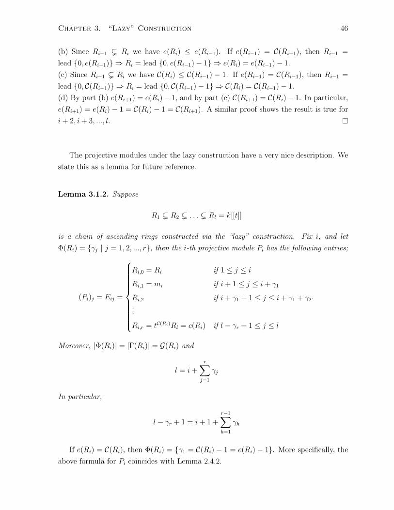
Lemma 3.1.2. Suppose
R1 ( R2 ( . . . ( Rl = k[[t]]
is a chain of ascending rings constructed via the “lazy” construction. Fix i, and let
Φ(Ri) = {γj | j = 1, 2, ..., r}, then the i-th projective module Pi has the following entries;
(Pi)j = Eij =
Ri,0 = Ri if 1 ≤ j ≤ i
Ri,1 = mi if i+ 1 ≤ j ≤ i+ γ1
Ri,2 if i+ γ1 + 1 ≤ j ≤ i+ γ1 + γ2·...
Ri,r = tC(Ri)Rl = c(Ri) if l − γr + 1 ≤ j ≤ l
Moreover, |Φ(Ri)| = |Γ(Ri)| = G(Ri) and
l = i+r∑j=1
γj
In particular,
l − γr + 1 = i+ 1 +r−1∑h=1
γh
If e(Ri) = C(Ri), then Φ(Ri) = {γ1 = C(Ri)− 1 = e(Ri)− 1}. More specifically, the
above formula for Pi coincides with Lemma 2.4.2.
Chapter 3. “Lazy” Construction 47
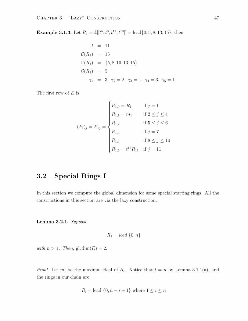
Example 3.1.3. Let R1 = k[[t5, t8, t17, t19]] = lead{0, 5, 8, 13, 15}, then
l = 11
C(R1) = 15
Γ(R1) = {5, 8, 10, 13, 15}
G(R1) = 5
γ1 = 3, γ2 = 2, γ3 = 1, γ4 = 3, γ5 = 1
The first row of E is
(P1)j = E1j =
R1,0 = R1 if j = 1
R1,1 = m1 if 2 ≤ j ≤ 4
R1,2 if 5 ≤ j ≤ 6
R1,3 if j = 7
R1,4 if 8 ≤ j ≤ 10
R1,5 = t15R11 if j = 11
3.2 Special Rings I
In this section we compute the global dimension for some special starting rings. All the
constructions in this section are via the lazy construction.
Lemma 3.2.1. Suppose
R1 = lead {0, n}
with n > 1. Then, gl. dim(E) = 2.
Proof. Let mi be the maximal ideal of Ri. Notice that l = n by Lemma 3.1.1(a), and
the rings in our chain are
Ri = lead {0, n− i+ 1} where 1 ≤ i ≤ n
Chapter 3. “Lazy” Construction 48
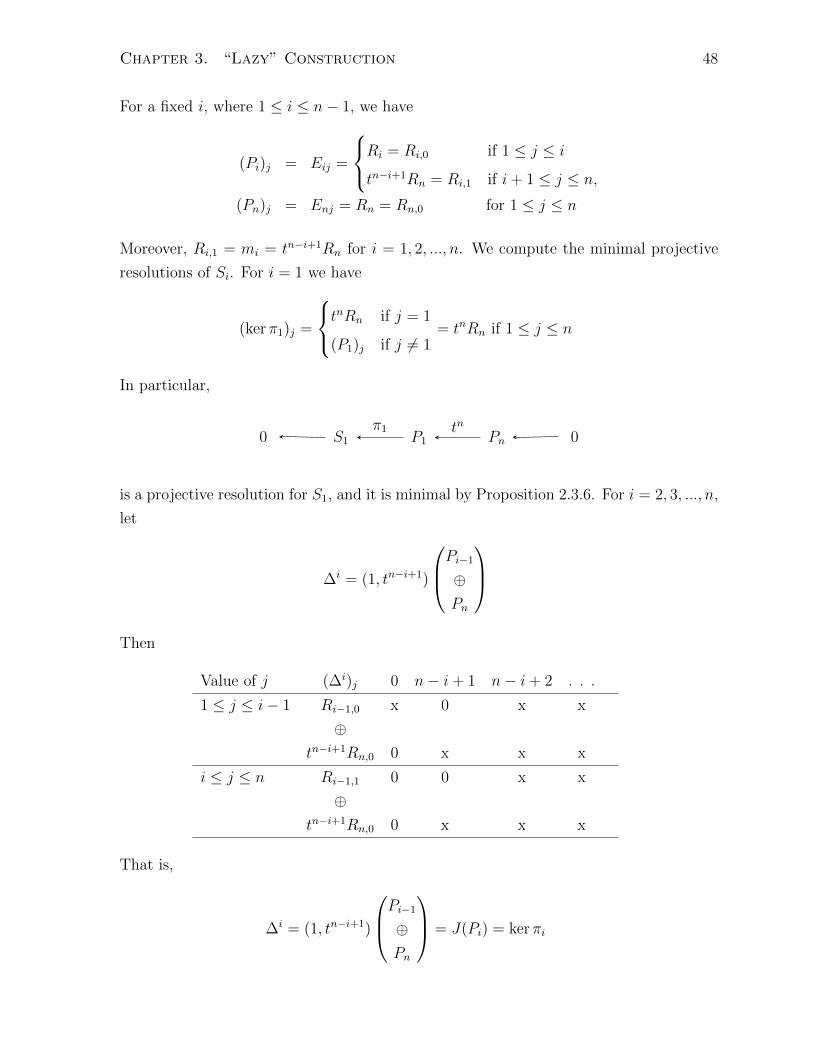
For a fixed i, where 1 ≤ i ≤ n− 1, we have
(Pi)j = Eij =
Ri = Ri,0 if 1 ≤ j ≤ i
tn−i+1Rn = Ri,1 if i+ 1 ≤ j ≤ n,
(Pn)j = Enj = Rn = Rn,0 for 1 ≤ j ≤ n
Moreover, Ri,1 = mi = tn−i+1Rn for i = 1, 2, ..., n. We compute the minimal projective
resolutions of Si. For i = 1 we have
(kerπ1)j =
tnRn if j = 1
(P1)j if j 6= 1= tnRn if 1 ≤ j ≤ n
In particular,
0 S1 P1 Pn 0π1 tn
is a projective resolution for S1, and it is minimal by Proposition 2.3.6. For i = 2, 3, ..., n,
let
∆i = (1, tn−i+1)
Pi−1⊕Pn
Then
Value of j (∆i)j 0 n− i+ 1 n− i+ 2 . . .
1 ≤ j ≤ i− 1 Ri−1,0 x 0 x x
⊕tn−i+1Rn,0 0 x x x
i ≤ j ≤ n Ri−1,1 0 0 x x
⊕tn−i+1Rn,0 0 x x x
That is,
∆i = (1, tn−i+1)
Pi−1⊕Pn
= J(Pi) = ker πi

Chapter 3. “Lazy” Construction 49
Moreover, ker(1, tn−i+1) has the following presentation:
Value of j 0 1 . . . n− i+ 1 n− i+ 2 . . .
1 ≤ j ≤ n 0 0 0 0 x x
0 x x x x x
Therefore,
0 Si Pi
Pi−1
⊕Pn
Pn 0πi (1, tn−i+1)
(tn−i+2
−t
)
is a projective resolutions for Si, and it is minimal by Proposition 2.3.6. The result
follows by Theorem 1.1.3.
An immediate consequence of Lemma 3.2.1 is: if e(R1) = C(R1), then gl. dim(E) =
2. Moreover, combining Lemma 3.1.1(d) with the proof in Lemma 3.2.1 shows that if
Ri−1 = lead {0, e(Ri−1)} for some 2 ≤ i ≤ l, then the minimal projective resolution of Si
is given by
0 Si Pi
Pi−1
⊕Pl
Pl 0πi (1, te(Ri))
(te(Ri−1)
−t
)
That is, pdE(Sj) = 2 for all j with i ≤ j ≤ l. This leads us to the following which we
present as a lemma for future reference.
Lemma 3.2.2. Suppose 2 ≤ i ≤ l with C(Ri−1) = e(Ri−1). Then,
(a) If e(R1) = C(R1) then gl. dim(E) = 2
(b) pdE(Sj) = 2 for all i ≤ j ≤ l.
(c) pdE(Sj) = 2 for z(R1) + 2 ≤ j ≤ l.
Proof. The only parts we need to prove is parts (c). This follows from the fact that
e(Rz(R1)+1)) = C(Rz(R1)+1)).
Lemma 3.2.3. Suppose b ∈ N, n > 1 with
R1 = lead {0, xn : x = 1, 2, ..., b}
Chapter 3. “Lazy” Construction 50
Then gl. dim(E) = 2.
Lemma 3.2.1 is a special case of this lemma (by setting b = 1).
Proof. The rings in our chain are
R2 = lead{0, xn, bn− 1 : x = 1, 2, ..., b− 1}
R3 = lead{0, xn, bn− 2 : x = 1, 2, ..., b− 1}...
Rb(n−1)+1 = lead {0, 1} = k[[t]]
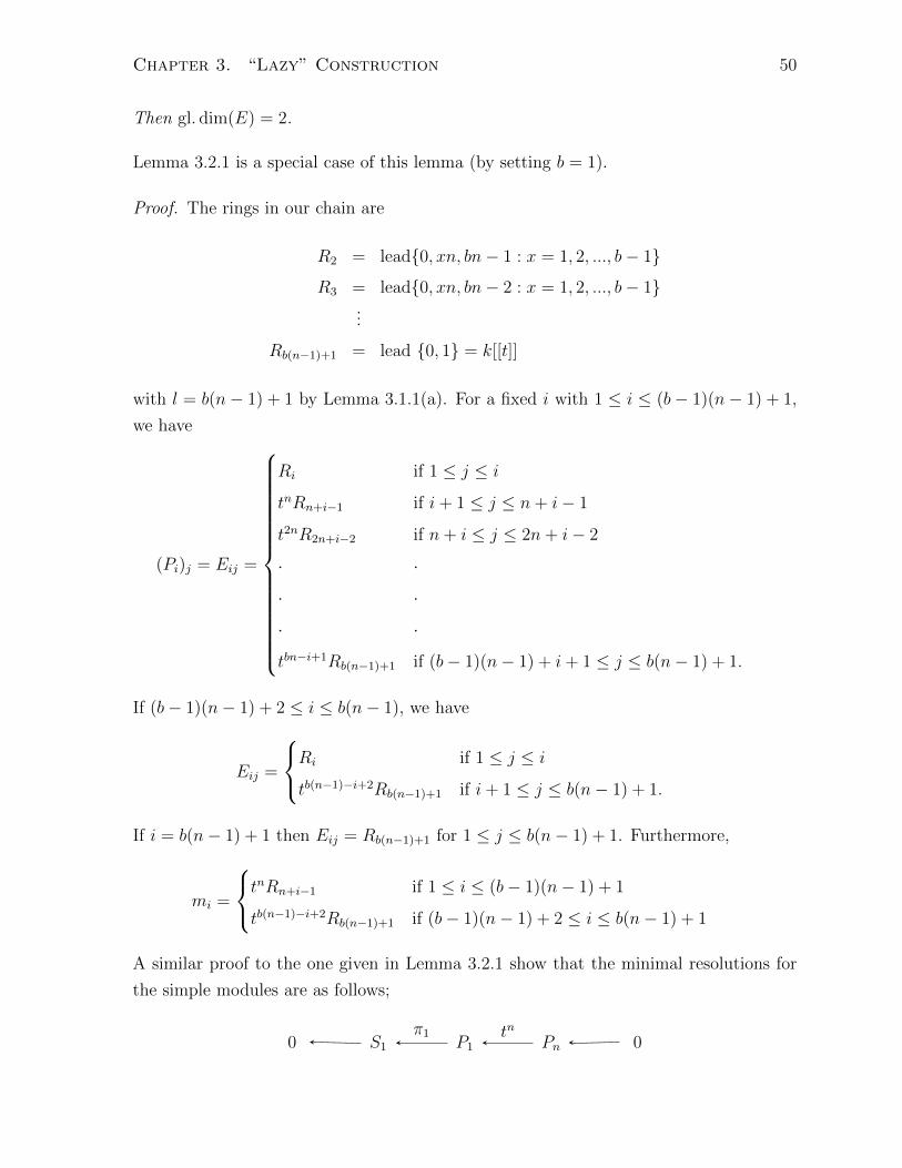
with l = b(n− 1) + 1 by Lemma 3.1.1(a). For a fixed i with 1 ≤ i ≤ (b− 1)(n− 1) + 1,
we have
(Pi)j = Eij =
Ri if 1 ≤ j ≤ i
tnRn+i−1 if i+ 1 ≤ j ≤ n+ i− 1
t2nR2n+i−2 if n+ i ≤ j ≤ 2n+ i− 2
· ·
· ·
· ·
tbn−i+1Rb(n−1)+1 if (b− 1)(n− 1) + i+ 1 ≤ j ≤ b(n− 1) + 1.
If (b− 1)(n− 1) + 2 ≤ i ≤ b(n− 1), we have
Eij =
Ri if 1 ≤ j ≤ i
tb(n−1)−i+2Rb(n−1)+1 if i+ 1 ≤ j ≤ b(n− 1) + 1.
If i = b(n− 1) + 1 then Eij = Rb(n−1)+1 for 1 ≤ j ≤ b(n− 1) + 1. Furthermore,
mi =
tnRn+i−1 if 1 ≤ i ≤ (b− 1)(n− 1) + 1
tb(n−1)−i+2Rb(n−1)+1 if (b− 1)(n− 1) + 2 ≤ i ≤ b(n− 1) + 1
A similar proof to the one given in Lemma 3.2.1 show that the minimal resolutions for
the simple modules are as follows;
0 S1 P1 Pn 0π1 tn

Chapter 3. “Lazy” Construction 51
For 2 ≤ i ≤ (b− 1)(n− 1) + 1
0 Si Pi
Pi−1
⊕Pn+i−1
Pn+i−2 0πi (1, tn))
(tn
−1
)
Let ρi = b(n− 1)− i+ 2. For (b− 1)(n− 1) + 2 ≤ i ≤ b(n− 1) + 1
0 Si Pi
Pi−1
⊕Pb(n−1)+1
Pb(n−1)+1 0πi (1, tρi)
(tρi+1
−t
)
The result follows by Theorem 1.1.3.
Lemma 3.2.4. Suppose b ∈ N, n > 1 with
R1 = lead {0, xn, bn+ c : x = 1, 2, ..., b}
where 1 < c ≤ n. Then gl. dim(E) = 2.
The case c = 1 is the preceding lemma (we don’t allow it here due to notational purposes).
Proof. Notice that l = b(n− 1) + c by Lemma 3.1.1(a), and the rings in our chain are
R2 = lead {0, xn, bn+ c− 1 : x = 1, 2, ..., b}
R3 = lead {0, xn, bn+ c− 2 : x = 1, 2, ..., b}...
Rb(n−1)+c = lead {0, 1} = k[[t]]
We give the minimal projective resolutions for the simple modules (the proof is similar
to the one given in Lemma 3.2.1);
0 S1 P1 Pn 0π1 tn
For 2 ≤ i ≤ (b− 1)(n− 1) + c

Chapter 3. “Lazy” Construction 52
0 Si Pi
Pi−1
⊕Pn+i−1
Pn+i−2 0πi (1, tn)
(tn
−1
)
Let ρi = b(n− 1) + c− i+ 1. For (b− 1)(n− 1) + c+ 1 ≤ i ≤ b(n− 1) + c
0 Si Pi
Pi−1
⊕Pb(n−1)+c
Pb(n−1)+c 0πi (1, tρi)
(tρi+1
−t
)
The result follows by Theorem 1.1.3.
The next lemmas gives us the first view of a starting ring that leads to an endomor-
phism ring with global dimension 3.
Lemma 3.2.5. Suppose n ≥ 3 and
R1 = lead {0, n, n+ 1, n+ 3}
then gl. dim(E) = 3.
Note that the result is false for n = 2. If n = 2 then n + 2 = 4 = 2n and tn+2 would be
in R1, which would give gl. dim(E) = 2 (Proposition 3.2.1).
Proof. Notice that l = n+1 by Lemma 3.1.1(a), and the rings in our chain are as follows:
R2 = lead {0, n}
R3 = lead {0, n− 1}...
Rn+1 = lead {0, 1} = k[[t]]
If i = n+ 1, then (Pi)j = Eij = Rn+1 for 1 ≤ j ≤ n+ 1. If 2 ≤ i ≤ n, then
(Pi)j = Eij =
Ri = Ri,0 if 1 ≤ j ≤ i
tn−i+2Rn+1 = mi = Ri,1 if i+ 1 ≤ j ≤ n+ 1,
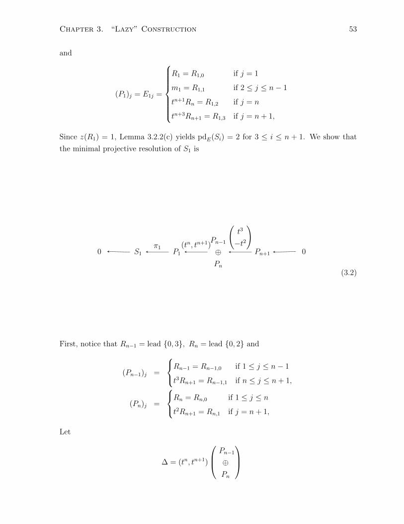
Chapter 3. “Lazy” Construction 53
and
(P1)j = E1j =
R1 = R1,0 if j = 1
m1 = R1,1 if 2 ≤ j ≤ n− 1
tn+1Rn = R1,2 if j = n
tn+3Rn+1 = R1,3 if j = n+ 1,
Since z(R1) = 1, Lemma 3.2.2(c) yields pdE(Si) = 2 for 3 ≤ i ≤ n + 1. We show that
the minimal projective resolution of S1 is
0 S1 P1
Pn−1
⊕Pn
Pn+1 0π1 (tn, tn+1)
(t3
−t2
)
(3.2)
First, notice that Rn−1 = lead {0, 3}, Rn = lead {0, 2} and
(Pn−1)j =
Rn−1 = Rn−1,0 if 1 ≤ j ≤ n− 1
t3Rn+1 = Rn−1,1 if n ≤ j ≤ n+ 1,
(Pn)j =
Rn = Rn,0 if 1 ≤ j ≤ n
t2Rn+1 = Rn,1 if j = n+ 1,
Let
∆ = (tn, tn+1)
Pn−1
⊕Pn

Chapter 3. “Lazy” Construction 54
Then the image of (tn, tn+1) has the following presentation:
Value of j ∆j n n+ 1 n+ 2 n+ 3 . . .
1 ≤ j ≤ n− 1 tnRn−1,0 x 0 0 x x
⊕tn+1Rn,0 0 x 0 x x
j = n tnRn−1,1 0 0 0 x x
⊕tn+1Rn,0 0 x 0 x x
j = n+ 1 tnRn−1,1 0 0 0 x x
⊕tn+1Rn,1 0 0 0 x x
That is, Im(tn, tn+1) = J(P1) = kerπ1. Furthermore, ker(tn, tn+1) has the following
presentation:
Value of j 0 1 2 3 . . .
1 ≤ j ≤ n 0 0 0 x x
0 0 x x x
That is
ker(tn, tn+1) =
(t3
−t2
)Pn+1 (
J(Pn−1)
⊕J(Pn)
= J
Pn−1⊕Pn
Therefore, (3.2) is a minimal projective resolution for S1. Now we show that the minimal
projective resolution for S2 is

Chapter 3. “Lazy” Construction 55
0 S2 P2
P1
⊕Pn+1
0 Pn+1
Pn−1
⊕Pn
π2 (1, tn)
(tn tn+1
−1 −t
)(t3
−t2
)
(3.3)
Let
∆′ = (1, tn)
P1
⊕Pn+1
Then the image of (1, tn) has the following presentation:
Value of j ∆′j 0 n n+ 1 n+ 2 n+ 3 . . .
j = 1 R1,0 x x x 0 x
⊕tnRn+1,0 0 x x x x
2 ≤ j ≤ n− 1 R1,1 0 x x 0 x
⊕tnRn+1,0 0 x x x x
j = n R1,2 0 0 x 0 x
⊕tnRn+1,0 0 x x x x
j = n+ 1 R1,3 0 0 0 0 x
⊕tnRn+1,0 0 x x x x

Chapter 3. “Lazy” Construction 56
That is Im(1, tn) = J(P2) = ker π2. Moreover, ker(1, tn) has the following presentation:
Value of j 0 1 2 . . . n n+ 1 n+ 2 n+ 3 . . .
1 ≤ j ≤ n− 1 0 0 0 0 x x 0 x x
x x 0 x x x x x x
j = n 0 0 0 0 0 x 0 x x
0 x 0 x x x x x x
j = n+ 1 0 0 0 0 0 0 0 x x
0 0 0 x x x x x x
A similar calculation to the ones done above show that
ker(1, tn) =
(tn tn+1
−1 −t
)Pn−1⊕Pn
(
J(P1)
⊕J(Pn+1)
= J
P1
⊕Pn+1
An element is in the kernel of a matrix if and only if it is in the kernel of each of its rows.
Since (tn, tn+1) = −tn(−1,−t), we have ker(tn, tn+1) = ker(−1,−t). But, we already
know ker(tn, tn+1) from the projective resolution of S1. In particular,
ker
(tn tn+1
−1 −t
)=
(t3
−t2
)Pn+1 (
J(Pn−1)
⊕J(Pn)
= J
Pn−1⊕Pn
In particular, (3.3) is a minimal projective resolution for S2, and the result follows by
Theorem 1.1.3.
Lemma 3.2.6. Suppose n ≥ 3 with
R1 = lead {0, n, n+ 1, 2n}
then gl. dim(E) = 3
.
Proof. The case n = 3 is taken care of by Lemma 3.2.5. Suppose n ≥ 4. Lemma 3.1.1(a)
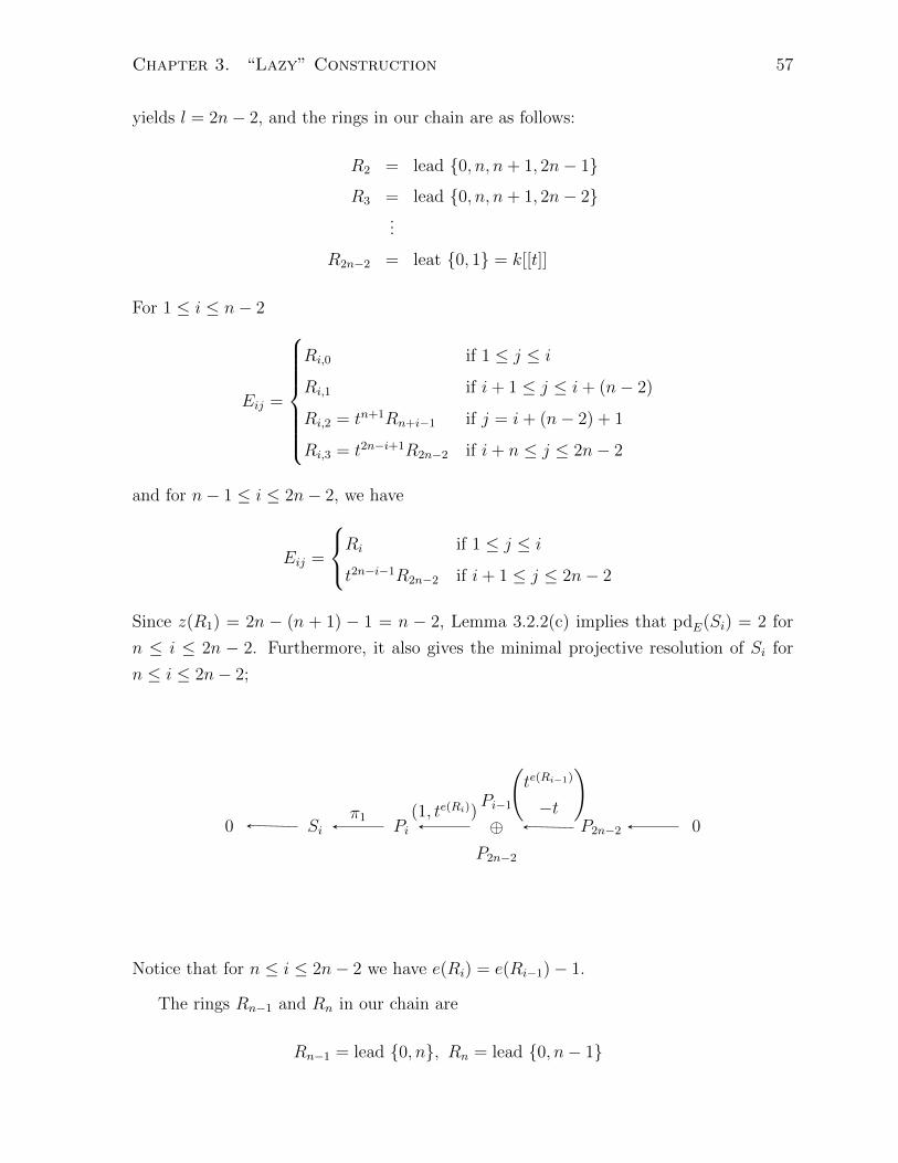
Chapter 3. “Lazy” Construction 57
yields l = 2n− 2, and the rings in our chain are as follows:
R2 = lead {0, n, n+ 1, 2n− 1}
R3 = lead {0, n, n+ 1, 2n− 2}...
R2n−2 = leat {0, 1} = k[[t]]
For 1 ≤ i ≤ n− 2
Eij =
Ri,0 if 1 ≤ j ≤ i
Ri,1 if i+ 1 ≤ j ≤ i+ (n− 2)
Ri,2 = tn+1Rn+i−1 if j = i+ (n− 2) + 1
Ri,3 = t2n−i+1R2n−2 if i+ n ≤ j ≤ 2n− 2
and for n− 1 ≤ i ≤ 2n− 2, we have
Eij =
Ri if 1 ≤ j ≤ i
t2n−i−1R2n−2 if i+ 1 ≤ j ≤ 2n− 2
Since z(R1) = 2n − (n + 1) − 1 = n − 2, Lemma 3.2.2(c) implies that pdE(Si) = 2 for
n ≤ i ≤ 2n − 2. Furthermore, it also gives the minimal projective resolution of Si for
n ≤ i ≤ 2n− 2;
0 Si Pi
Pi−1
⊕P2n−2
P2n−2 0π1 (1, te(Ri))
(te(Ri−1)
−t
)
Notice that for n ≤ i ≤ 2n− 2 we have e(Ri) = e(Ri−1)− 1.
The rings Rn−1 and Rn in our chain are
Rn−1 = lead {0, n}, Rn = lead {0, n− 1}

Chapter 3. “Lazy” Construction 58
This yields
(J(P1))j =
R1,1 if 1 ≤ j ≤ n− 1
R1,2 if j = n
R1,3 if n+ 1 ≤ j ≤ 2n
(Pn−1)j =
Rn−1,0 if 1 ≤ j ≤ n− 1
Rn−1,1 if n ≤ j ≤ 2n− 2
(Pn)j =
Rn,0 if 1 ≤ j ≤ n
Rn,1 if n+ 1 ≤ j ≤ 2n− 2
Let
∆ = (tn, tn+1)
Pn−1⊕Pn
then the image of (tn, tn+1) has the following presentation:
Values of j ∆j n n+ 1 2n . . .
1 ≤ j ≤ n− 1 tnRn−1,0 x 0 x . . .
⊕tn+1Rn,0 0 x x . . .
j = n tnRn−1,1 0 0 x . . .
⊕tn+1Rn,0 0 x x . . .
n+ 1 ≤ j ≤ 2n− 2 tnRn−1,1 0 0 x . . .
⊕tn+1Rn+1,1 0 0 x . . .
That is, Im(tn, tn+1) = J(P1) = ker π1. The ker(tn, tn+1) has the following presentation:
Values of j n− 1 n . . .
1 ≤ j ≤ 2n− 2 0 x . . .
x x . . .

Chapter 3. “Lazy” Construction 59
That is,
ker(tn, tn+1) =
(tn
−tn−1
)P2n−2 ( J
Pn−1
⊕P2n−2
Hence,
0 S1 P1
Pn−1
⊕Pn
P2n−2 0π1 (tn, tn+1)
(tn
−tn−1
)
is a minimal projective resolution of S1.
A similar computation to the one above gives the minimal resolutions of Si for 2 ≤ i ≤n− 1, and they are as follows:
0 Sn−1 Pn−1
Pn−2
⊕P2n−2
0 P2n−2
P2n−4
⊕P2n−3
πn−1 (1, tn)
(tn tn+1
−1 −t
)(t3
−t2
)
and for 2 ≤ i ≤ n− 2

Chapter 3. “Lazy” Construction 60
0 Si Pi
Pi−1
⊕Pn−i+2
⊕Pn−i+3
0 P2n−2
Pn−i+1
⊕Pn−i+2
⊕P2n−2
πi (1, tn, tn+1)
−tn −tn+1 0
1 0 −tn−i+1
0 1 tn−i
tn−i+2
−tn−i+1
t
The result follows by Theorem 1.1.3.
3.3 Minor Results I
Since Ri+1 = Ri[[tC(Ri)−1]] for 1 ≤ i ≤ l − 1, the largest powers of t missing from Ri
is “forced” in to construct Ri+1 and no other powers of t are “forced” in. This process
starts by “forcing” in the largest power of t missing from R1. This proves the following
lemma.
Lemma 3.3.1. If e(Rj) < e(R1) for some 2 ≤ j ≤ l, then G(Rj) = 1.
The following proposition shows that the global dimension of the endomorphism ring
is completely determined when the projective dimension of the first simple module is one.
Proposition 3.3.2. Suppose pdE(S1) = 1, then gl. dim(E) = 2 = pdE(Sj), for any
2 ≤ j ≤ l.
Proof. Let e(R1) = n > 1 and G(R1) = r. Consider the intervals a1(R1), a2(R1), ..., ar(R1)
for R1. Recall that r ≥ 1 . If r = 1, then
R1 = lead {0, n}
and Lemma 3.2.1 gives us the desired result.
If r ≥ 2, then a1(R1) = n − 1 ≥ a2(R1). Since pdE(S1) = 1 we have the following
projective resolution for S1;

Chapter 3. “Lazy” Construction 61
0 S1 P1 Pj 0π1 tn
for some 1 ≤ j ≤ l. This gives the following exact sequence;
0 k = R1/m1 R1 Rj 0ξ1 tn
Thus, tnRj = m1. Notice that 1 < j ≤ l by Proposition 2.2.14(d). Moreover,
tb ∈ Rj ⇔ tb+n ∈ m1
In particular,
ai(Rj) = ai+1(R1) and G(Rj) = r − 1
Suppose a1(R1) > a2(R1). Then
a1(Rj) = a2(R1) < n− 1 < e(R1)⇒ e(Rj) < e(R1)
and G(Rj) = 1 by Lemma 3.3.1, which in turn yields r = 2. That is,
R1 = lead {0, n, n+ c} with 1 < c < n,
and the result follows by Lemma 3.2.4.
If a1(R1) = a2(R1), then r ≥ 2. If r = 2 the result follows by Lemma 3.2.3. Suppose
r > 2, then we have a2(R1) = n− 1 ≥ a3(R1). If a3(R1) < n− 1 we show that r = 3. Let
Γ(R1) = {β1, β2, . . . , βr} and Γ(Rj) = {α1, α2, . . . , αr−1}
then β1 = n, β2 = 2n, and β3 = 2n + c for some 1 < c < n. If r ≥ 4, then 2n + c + 2 ≤β4 ≤ 3n and this implies that
α1 = β2 − n = n, α2 = β3 − n = n+ c, α3 = β4 − n
where n + c + 2 ≤ α3 ≤ 2n. That is, the first four powers of t that appear in Rj are
0, n, n + c,and α3. However, since the rings were constructed via the lazy construction
no such ring exists in our chain, a contradiction. Hence, r = 3 and
R1 = lead {0, n, 2n, 2n+ c},

Chapter 3. “Lazy” Construction 62
and the result follows by Lemma 3.2.4. If a1(R1) = a2(R1) = a3(R1), we repeat the
preceding argument and continue this until we get to ar(R1). In particular, we have the
following two possible cases;
Case 1. a1(R1) = a2(R1) = ... = ar(R1). In this case
R1 = lead {0, xn : x = 1, 2, ..., r},
and the result follows by Lemma 3.2.3,
or
Case 2. a1(R1) = a2(R1) = ... = ar−1(R1) > ar(R1). In this case
R1 = lead {0, xn, (r − 1)n+ c : x = 1, 2, ..., r − 1}
where 1 < c < n, and the result follows by Lemma 3.2.4.
Next we focus on how the projective resolutions of the simple modules begin under
the lazy construction.
Proposition 3.3.3. Let
R1 ( R2 ( . . . ( Rl = k[[t]]
be a chain of ascending rings constructed via the lazy construction with e(R1) = n > 1.
(a) If C(R1) = e(R1) := n > 1, then the minimal projective resolution of S1 is given by;
0 S1 P1 Pn 0π1 tn
(b) If 2 ≤ i ≤ l and e(Ri) = C(Ri), then the minimal projective resolution of Si has the
following beginning;
0 Si Pi
Pi−1
⊕Pl
· · ·πi (1, te(Ri))
Proof. (a) If C(R1) = n then
R1 = lead {0, n},

Chapter 3. “Lazy” Construction 63
the result follows by Lemma 3.2.1.
(b) For i = l the result follows from Proposition 2.4.3. Suppose 2 ≤ i ≤ l − 1. Since
e(Ri) = C(Ri) then Ri = lead{0, e(Ri)} with e(Ri) ≥ 2. and
Ri−1 = lead{0, e(Ri), e(Ri) + 1, . . . , e(Ri) + c, e(Ri) + c+ 2},
where 0 ≤ c ≤ e(Ri)− 2. In particular,
(Pi)j =
Ri if 1 ≤ j ≤ i
mi if i+ 1 ≤ j ≤ l
(Pi−1)j =
Ri−1 if 1 ≤ j ≤ i− 1
mi−1 if j = i (Lemma 2.4.1(e))
HomR1(Rj, Ri−1) if i+ 1 ≤ j ≤ l
By Lemma 2.4.1(b), (Pi−1)j ⊆ (Pi)j for 1 ≤ j ≤ l, and combining this with mi = te(Ri)Rl
yields
(1, te(Ri))
Pi−1⊕Pl
j
=
Ri if 1 ≤ j ≤ i− 1
mi if i ≤ j ≤ l= (J(Pi))j = (ker πi)j,
completing the proof.
Conjecture 1. If C(R1) > n, then the minimal projective resolution of S1 has the
following beginning;
0 S1 P1
⊕sa=1 Pλa . . .
π1 ζ
where Λ(R1) = {α1, ..., αs}, χ(R1) = {λ1, ..., λs}, and ζ = (tα1 , ..., tαs).
Proposition 3.3.4. Suppose conjecture 1 is true and 2 ≤ i ≤ l. If e(Ri) < C(Ri), then
the projective resolution of Si has the following beginning;
0 Si Pi
Pi−1
⊕⊕sa=1 Pλa
· · ·πi τi
where Λ(Ri) = {α1, ..., αs}, χ(Ri) = {λ1, ..., λs}, and τi = (1, tα1 , ..., tαs).
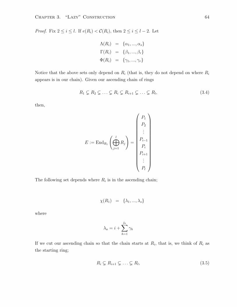
Chapter 3. “Lazy” Construction 64
Proof. Fix 2 ≤ i ≤ l. If e(Ri) < C(Ri), then 2 ≤ i ≤ l − 2. Let
Λ(Ri) = {α1, ..., αs}
Γ(Ri) = {β1, ..., βr}
Φ(Ri) = {γ1, ..., γr}
Notice that the above sets only depend on Ri (that is, they do not depend on where Ri
appears is in our chain). Given our ascending chain of rings
R1 ( R2 ( . . . ( Ri ( Ri+1 ( . . . ( Rl, (3.4)
then,
E := EndR1
(l⊕
j=1
Rj
)=
P1
P2
...
Pi−1
Pi
Pi+1
...
Pl
The following set depends where Ri is in the ascending chain;
χ(R1) = {λ1, ..., λs}
where
λa = i+
ja∑h=1
γh
If we cut our ascending chain so that the chain starts at Ri, that is, we think of Ri as
the starting ring;
Ri ( Ri+1 ( . . . ( Rl, (3.5)

Chapter 3. “Lazy” Construction 65
then,
E ′ := EndR1
(l⊕j=i
Rj
)= EndRi
(l⊕j=i
Rj
)=
P ′i
P ′i+1...
P ′l
is a l − (i− 1)× l − (i− 1) matrix with P ′jdi− 1e = Pj for i ≤ j ≤ l. Furthermore,
(P ′i )j =
Ri if j = 1
HomR1(Rj, Ri) if 2 ≤ j ≤ l − (i− 1)
=
Ri if j = 1
HomRi(Rj, Ri) if 2 ≤ j ≤ l − (i− 1)
By conjecture 1, the beginning of the minimal projective resolution of P ′i is given by;
0 S ′i P ′i⊕s
a=1 P′λ′a
· · ·π′i ζ
where
ζ = (tα1 , tα2 , . . . , tαs)
λ′a = 1 +
ja∑h=1
γh
(S ′i)j =
k if j = 1
0 if 2 ≤ j ≤ l − (i− 1)
(π′i)j =
ξi if j = 1
0 if 2 ≤ j ≤ l − (i− 1)
with ξi : Ri → k = Ri/mi is the natural map. This yields the following exact sequence
0 J(P ′i )⊕s
a=1 P′λ′a
· · ·ζ

Chapter 3. “Lazy” Construction 66
Lemma 2.6.5 yields the following exact sequence;
0 (J(P ′i ))di− 1e⊕s
a=1 P′λ′adi− 1e · · ·
ζ
(3.6)
Notice that λ′a are obtained from the ascending chain given in (3.5), which is the one
with Ri as the starting ring. To convert these subscripts when R1 is the starting ring
(the ascending chain given in (3.4)) we need to add i− 1 to these subscripts (since i− 1
rings are removed when Ri is the starting ring). More precisely, the exact sequence in
(3.6) becomes the following when R1 is the starting ring;
0 (J(P ′i ))di− 1e⊕s
a=1 P′λ′a+(i−1)di− 1e · · ·
ζ
(3.7)
Since
λ′a + (i− 1) = 1 +
ja∑h=1
γh + i− 1 = λa
the sequence in (3.7) becomes
0 (J(P ′i ))di− 1e⊕s
a=1 P′λadi− 1e · · ·
⊕sa=1 Pλa
ζ
(3.8)
Observe that
Im(ζ) = ((J(P ′i )di− 1e)j =
mi if 1 ≤ j ≤ i
HomR1(Rj, Ri) if i+ 1 ≤ j ≤ l
By Lemma 2.4.1(b), (Pi−1)j ⊆ (Pi)j for 1 ≤ j ≤ l. Combining this with the sequence in
(3.8) gives us the following beginning to the minimal projective resolution of Si;

Chapter 3. “Lazy” Construction 67
0 Si Pi
Pi−1
⊕⊕sa=1 Pλa
· · ·πi τi = (1, ζ)
as desired.
3.4 gl. dim(E) for l = 1, 2, 3, 4, 5
Our goal in this section is to compute the global dimension of E for small values of l.
More specifically, we compute gl. dim(E) for l = 1, 2, 3, 4, 5. If l = 1, then R1 = k[[t]]
and E = EndR1(R1) = R1. In particular, gl. dim(E) = 1 by Proposition 1.1.2.
Lemma 3.4.1. If l = 2, then gl. dim(E) = 2.
Proof. Since R2 = k[[t]] we have R1 = k[[t2, t3]] and the result follows by Lemma 3.2.1.
Lemma 3.4.2. If l = 3, then gl. dim(E) = 2.
Proof. There are two possible cases for R1;
R1 = k[[t3, t4, t5]] ⇒ gl. dim(E) = 2 (Lemma 3.2.1)
R1 = k[[t2, t5]] ⇒ gl. dim(E) = 2 (Lemma 3.2.3)
Lemma 3.4.3. If l = 4, then gl. dim(E) = 2 or 3.
Proof. There are three possibilities for R1;
R1 = k[[t4, t5, t6, t7]] ⇒ gl. dim(E) = 2 (Lemma 3.2.1)
R1 = k[[t2, t7]] ⇒ gl. dim(E) = 2 (Lemma 3.2.3)
R1 = k[[t3, t4]] ⇒ gl. dim(E) = 3 (Lemma 3.2.5)
Lemma 3.4.4. If l = 5, then gl. dim(E) = 2 or 3.
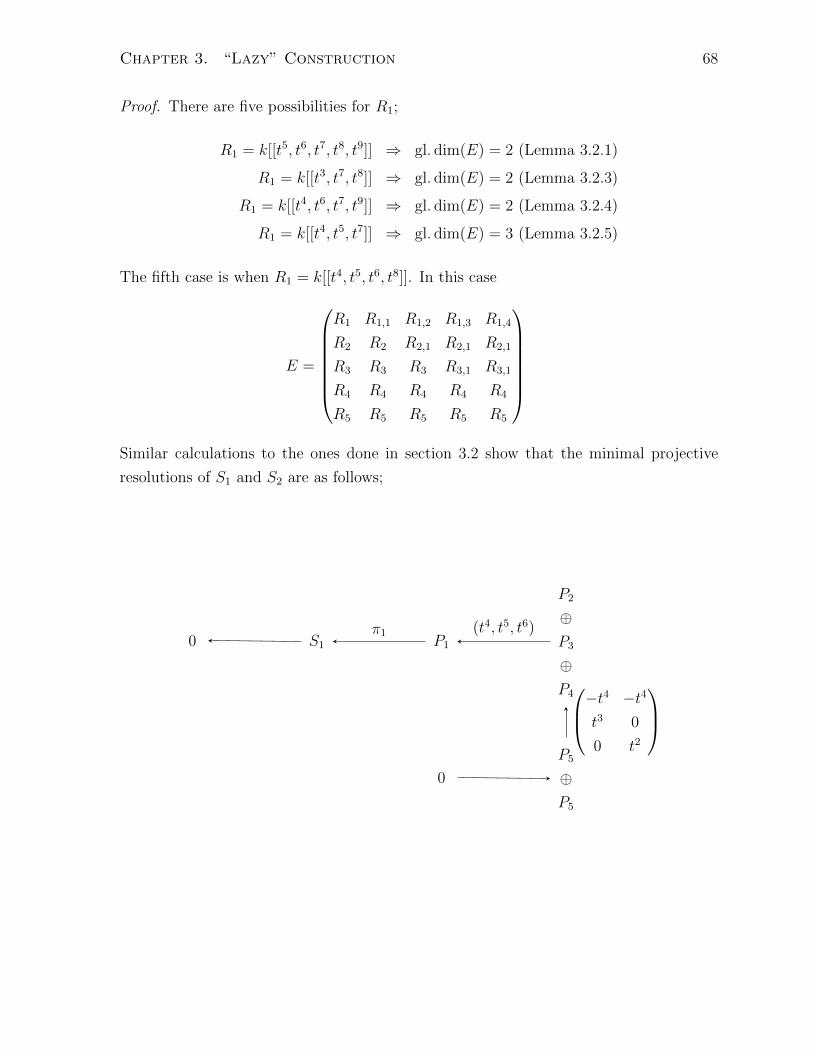
Chapter 3. “Lazy” Construction 68
Proof. There are five possibilities for R1;
R1 = k[[t5, t6, t7, t8, t9]] ⇒ gl. dim(E) = 2 (Lemma 3.2.1)
R1 = k[[t3, t7, t8]] ⇒ gl. dim(E) = 2 (Lemma 3.2.3)
R1 = k[[t4, t6, t7, t9]] ⇒ gl. dim(E) = 2 (Lemma 3.2.4)
R1 = k[[t4, t5, t7]] ⇒ gl. dim(E) = 3 (Lemma 3.2.5)
The fifth case is when R1 = k[[t4, t5, t6, t8]]. In this case
E =
R1 R1,1 R1,2 R1,3 R1,4
R2 R2 R2,1 R2,1 R2,1
R3 R3 R3 R3,1 R3,1
R4 R4 R4 R4 R4
R5 R5 R5 R5 R5
Similar calculations to the ones done in section 3.2 show that the minimal projective
resolutions of S1 and S2 are as follows;
0 S1 P1
P2
⊕P3
⊕P4
0
P5
⊕P5
π1 (t4, t5, t6)
−t4 −t4
t3 0
0 t2

Chapter 3. “Lazy” Construction 69
0 S2 P2
P1
⊕P5
P2
⊕P3
⊕P4
0
P5
⊕P5
π1 (1, t4)
(t4 t5 t6
−1 −t −t2
)
−t4 −t4
t3 0
0 t2
Moreover, since z(R1) = 1 we have pdE(Si) = 2 for 3 ≤ i ≤ 5 (Lemma 3.2.2). Hence,
gl. dim(E) = 3 by Theorem 1.1.3.
3.5 Constructing Endomorphism Rings of Large Global
Dimension
Throughout this section {Ri1 : i ∈ N} is a set of starting rings constructed in section 2.5
and for each natural number i, the ascending chain
Ri1 ( Ri
2 ( . . . ( Rili
= k[[t]]
is constructed via the lazy construction. We define
M i =
li⊕j=1
Rij and Ei = EndRi
1(M i)
In section 3.5.1 we investigate the lengths of the chains, projective modules, and the
projective dimension of the first simple modules for i = 1, 2. Once this is done, this
forms the backbone of the proofs of the main results in this chapter. In section 3.5.2
the first main result of this thesis is proved: we establish a lower bound for the global
dimension of Ei for each i ∈ N. Section 3.5.3 focuses on the module we get when we
remove the starting ring from our chain and instead start our chain from the second ring.
We conclude this section by proving the second main result of this thesis in section 3.5.4.
More precisely, we compute the global dimensions of Ei for a given set of starting rings.

Chapter 3. “Lazy” Construction 70
3.5.1 Minor Results II
This section is devoted to building the machinery needed in the next three sections. The
following proposition gives us a formula for li, the length of the chain with starting ring
Ri1.
Lemma 3.5.1. Given an even integer n ≥ 6, then l1 =3n
2− 1 and for i ≥ 2
li = i(n
2− 1)
+ C(R21)− n = C(R2
1) + (i− 2)n
2− i
Moreover,
li+1 = li +n
2− 1 for i ≥ 2
Proof.
l1 = 1 + g(R11) (Lemma 3.1.1)
= 1 + a1(R11) + a2(R
11)
= 1 + (n− 1) +(n
2− 1)
(Lemma 2.5.5)
=3n
2− 1
and for i ≥ 2,
li = 1 + g(Ri1) (Lemma 3.1.1)
= 1 +
G(Ri1)∑
j=1
aj(Ri1)
= 1 +i+1∑j=1
aj(Ri1) (Lemma 2.5.2)
= 1 + a1(Ri1) +
i∑j=2
aj(Ri1) + ai+1(R
i1)
= 1 + (n− 1) + (i− 1)(n
2− 1)
+ C(R21)−
3n
2− 1 (Lemma 2.5.5)
= i(n
2− 1)
+ C(R21)− n
= C(R21) + (i− 2)
n
2− i

Chapter 3. “Lazy” Construction 71
In particular, for i ≥ 2
li+1 = (i+ 1)(n
2− 1)
+ C(R21)− n
= i(n
2− 1)
+ C(R21)− n+
n
2− 1
= li +n
2− 1
Notice that l2 is not necessarily equal to l1 + n2− 1. To see this, the preceding
proposition yields
l2 = C(R21)− 2 and l1 +
n
2− 1 =
3n
2− 1 +
n
2− 1 = 2n− 2.
That is, the two are equal if and only if C(R21) = 2n (which is not true in general). The
following proposition allows us to go back and forth between the projective Ei modules
and projective Ei+1 modules. It plays a fundamental role in the main theorems we prove
later on in this thesis.
Proposition 3.5.2. Given an even integer n ≥ 6, let {Ri1 | i ∈ N} be a set of starting
rings constructed in section 2.5. Then
(a) For a given i ≥ 2 and j = 1, 2, ..., li,
(P i+1n2+j−1)a = (P i
j )a−n2+1 if n
2≤ a ≤ li+1
In particular, for i ≥ 2,
(P i+1n2
)a = (P i1)a−n
2+1 if n
2≤ a ≤ li+1
(b) For a given i ≥ 2 and j = 1, 2, ..., li,
(P i+1n2+j−1)a =
Rij if 1 ≤ a ≤ n
2− 1
(P ij )a−n
2+1 if n
2≤ a ≤ li+1
=((P ij
⌈n2− 1⌉))
a
In particular, for i ≥ 2,
(P i+1n/2 )a =
Ri1 if 1 ≤ a ≤ (n/2)− 1
(P i1)a−(n/2)+1 if (n/2) ≤ a ≤ li+1
=((P i1
⌈n2− 1⌉))
a
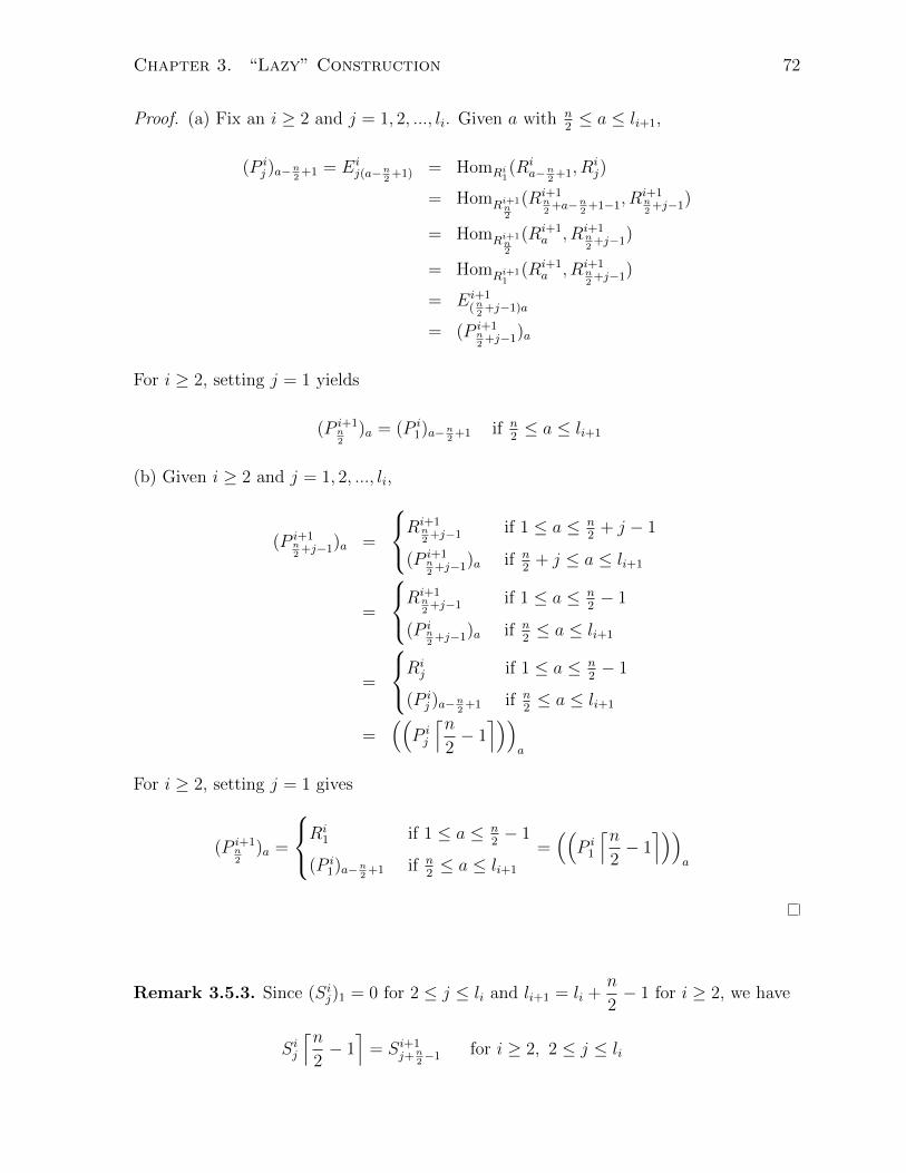
Chapter 3. “Lazy” Construction 72
Proof. (a) Fix an i ≥ 2 and j = 1, 2, ..., li. Given a with n2≤ a ≤ li+1,
(P ij )a−n
2+1 = Ei
j(a−n2+1) = HomRi
1(Ri
a−n2+1, R
ij)
= HomRi+1n2
(Ri+1n2+a−n
2+1−1, R
i+1n2+j−1)
= HomRi+1n2
(Ri+1a , Ri+1
n2+j−1)
= HomRi+11
(Ri+1a , Ri+1
n2+j−1)
= Ei+1(n2+j−1)a
= (P i+1n2+j−1)a
For i ≥ 2, setting j = 1 yields
(P i+1n2
)a = (P i1)a−n
2+1 if n
2≤ a ≤ li+1
(b) Given i ≥ 2 and j = 1, 2, ..., li,
(P i+1n2+j−1)a =
Ri+1n2+j−1 if 1 ≤ a ≤ n
2+ j − 1
(P i+1n2+j−1)a if n
2+ j ≤ a ≤ li+1
=
Ri+1n2+j−1 if 1 ≤ a ≤ n
2− 1
(P in2+j−1)a if n
2≤ a ≤ li+1
=
Rij if 1 ≤ a ≤ n
2− 1
(P ij )a−n
2+1 if n
2≤ a ≤ li+1
=((P ij
⌈n2− 1⌉))
a
For i ≥ 2, setting j = 1 gives
(P i+1n2
)a =
Ri1 if 1 ≤ a ≤ n
2− 1
(P i1)a−n
2+1 if n
2≤ a ≤ li+1
=((P i1
⌈n2− 1⌉))
a
Remark 3.5.3. Since (Sij)1 = 0 for 2 ≤ j ≤ li and li+1 = li +n
2− 1 for i ≥ 2, we have
Sij
⌈n2− 1⌉
= Si+1j+n
2−1 for i ≥ 2, 2 ≤ j ≤ li

Chapter 3. “Lazy” Construction 73
A consequence of Proposition 3.5.2 is
P 3q+2n−1 = P 3q+1
n2
⌈n2− 1⌉
= P 3q1 [n− 2]
P 3q+23n2−2 = P 3q+1
n−1
⌈n2− 1⌉
= P 3qn2dn− 2e = P 3q−1
1
⌈3n
2− 3
⌉for q ≥ 1. We conclude this section by computing the projective dimension of S1
1 as an
E1-module and S21 as an E2-module.
Lemma 3.5.4. pdE1(S11) = 1 and gl. dim(E1) = 2.
Proof. By Lemma 3.2.4
0 S11 P 1
1 P 1n 0
π11 tn
is the minimal projective resolution of S11 . That is, pdE1(S1
1) = 1. The second part
follows by Proposition 3.3.2.
The following notation will be very useful throughout this thesis.
Notation 3.5.5. Let
ε = C(R21)−
3n
2, ε1 = C(R2
1)− n, ε2 = C(R21)−
n
2
ζ = (tn, t3n2 ), τ =
(t3n2 t2n
−tn −t 3n2
):=
(τ1
τ2
), φ =
(tε1
−tε
)
Notice that
ζτ = 0, τφ = 0, ζφ = 0, τ1φ = 0, τ2φ = 0
Lemma 3.5.6. The minimal projective resolution of S21 is as follows;
0 S21 P 2
1
P 2n−1
⊕P 2
3n2−1
P 2l2
0π21 ζ φ
(3.9)
In particular, pdE2(S21) = 2.

Chapter 3. “Lazy” Construction 74
Proof. Since
R21 = lead
{0, n,
3n
2, C(R2
1)
}R2n−1 = lead {0, ε1}
R23n2−1 = lead {0, ε}
R2l2
= k[[t]]
Lemma 3.1.2 yields
(P 21 )j =
R21,0 = R2
1 if j = 1
R21,1 = m2
1 if 2 ≤ j ≤ n− 1
R21,2 if n ≤ j ≤ 3n
2− 1
R21,3 if 3n
2≤ j ≤ l2
(P 2n−1)j =
R2n−1,0 = R2
n−1 if 1 ≤ j ≤ n− 1
R2n−1,1 = m2
n−1 = tε1R2l2
if n ≤ j ≤ l2
(P 23n2−1)j =
R23n2−1,0 = R2
3n2−1 if 1 ≤ j ≤ 3n
2− 1
R23n2−1,1 = m2
3n2−1 = tεR2
l2if 3n
2≤ j ≤ l2
and (P 2l2
)j = R2l2
= k[[t]] for 1 ≤ j ≤ l2. Let
∆ = (tn, t3n2 )
P 2n−1
⊕P 2
3n2−1

Chapter 3. “Lazy” Construction 75
This gives us the following table;
Value of j ∆j n 3n2C(R2
1) . . .
1 ≤ j ≤ n− 1 tnR2n−1 x 0 x x
⊕t3n2 R2
3n2−1 0 x x x
n ≤ j ≤ 3n2− 1 tnm2
n−1 0 0 x x
⊕t3n2 R2
3n1−1 0 x x x
3n2≤ j ≤ l2 tnm2
n−1 0 0 x x
⊕t3n2 m2
3n2−1 0 0 x x
Therefore, ker ζ has the following representation;
Value of j ε ε+ 1 . . . ε1 . . .
1 ≤ j ≤ l2 0 0 0 x x
x x x x x
That is,
(tn, t3n2 )
P 2n−1
⊕P 2
3n2−1
= J(P 21 ) = ker π2
1
and
φ(P 2l2
) = ker
P 2n−1
⊕P 2(3n/2)−1
ζ−→ P 21
(
J(P 2n−1)
⊕J(P 2
(3n/2)−1)
= J
P 2n−1
⊕P 2(3n/2)−1
Hence, (3.9) is a projective resolution for S2
1 (it is minimal by Proposition 2.3.6), com-
pleting the proof.
3.5.2 Lower Bound for gl. dim(Ei)
In this section we prove the first main result of this thesis. More precisely, we obtain a
lower bound for the global dimension of Ei. We begin with a useful definition.

Chapter 3. “Lazy” Construction 76
Definition 3.5.7. Let n be a positive even integer and a ≤ b be non-negative integers,
we define
Aba(n) ={xn
2: x = a, a+ 1, ..., b
}
Now we are in position to prove the first main result of this thesis.
Theorem 3.5.8. Let {Ri1|i ∈ N} be a set of starting rings constructed in section 2.5.
(a) If q ≥ 1, then
0 S3q+21 P 3q+2
1
P 3q+2n−1
⊕P 3q+2
3n2−2
(J(P 3q−11 ))
⌈3n2− 3⌉
0π3q+21 ζ µ
(3.10)
is an exact sequence, where
µ =
(tn2
−1
), Im(ζ) = J(P 3q+2
1 )
(b) If q ≥ 0, then
0 S3q+21 W0 W1 W2 · · · Wq+1 Wq+2 0
d0 d1 d2 d3 dq+1 dq+2
(3.11)

Chapter 3. “Lazy” Construction 77
is a minimal projective resolution for S3q+21 , where
Wj =
P 3q+21 if j = 0
P 3q+2(n−1)+3(j−1)(n
2−1)
⊕
P 3q+2(n−1)+3(j−1)(n
2−1)+(n
2−1)
if j = 1, 2, ..., q
P 3q+2(n−1)+3q(n
2−1)
⊕
P 3q+2(n−1)+3q(n
2−1)+n
2
if j = q + 1
P 3q+2l3q+2
if j = q + 2
and
dj =
π3q+21 if j = 0
ζ if j = 1
τ for j = 2, ..., q + 1
φ if j = q + 2
In particular, pdE3q+2(S3q+21 ) = q + 2 for q ∈ N0 ⇒ gl. dim(E3q+2) ≥ q + 2 for q ∈ N0.
Notice that if q = 0 the second row for Wj above is omitted.
Proof. (a) Fix q ≥ 1, definition 2.5.1 and the lazy construction yield
R3q+21 = lead
{0,jn
2, C(R3q+2
1 ) : j = 2, 3, ..., 3q + 3
}R3q+2n−1 = lead
{0,jn
2, C(R3q+2
n−1 ) : j = 2, 3, ..., 3q + 1
}R3q+2
3n2−2 = lead
{0,jn
2, C(R3q+2
3n2−2
): j = 2, 3, ..., 3q
}

Chapter 3. “Lazy” Construction 78
where
C(R3q+2n−1 ) = C(R3q+2
1 )− n
C(R3q+2
3n2−2
)= C(R3q+2
1 )− 3n
2
and
G(R3q+21 ) = 3q + 3
G(R3q+2n−1 ) = G(R3q+2
1 )− 2 = 3q + 1
G(R3q+2
3n2−2
)= G(R3q+2
1 )− 3 = 3q
Lemmas 3.1.2 and 2.5.8 yield
(P 3q+21 )j =
R3q+21,0 if j = 1
R3q+21,1 if 2 ≤ j ≤ n− 1
R3q+21,2 if n ≤ j ≤ 3n
2− 2
R3q+21,3 if 3n
2− 1 ≤ j ≤ 2n− 3
R3q+21,a if an
2− a+ 2 ≤ j ≤ (a+1)n
2− a for 2 ≤ a ≤ 3q + 1
R3q+21,3q+2 if (3q+2)n
2− 3q ≤ j ≤ (3q+3)n
2− (3q + 1)
R3q+21,3q+3 if (3q+3)n
2− 3q ≤ j ≤ l3q+2
(P 3q+2n−1 )j =
R3q+2n−1,0 if 1 ≤ j ≤ n− 1
R3q+2n−1,1 if n ≤ j ≤ 2n− 3
R3q+2n−1,2 if 2n− 2 ≤ j ≤ 5n
2− 4
R3q+2n−1,3 if 5n
2− 3 ≤ j ≤ 3n− 5
R3q+2n−1,a if an
2+ n− a ≤ j ≤ (a+3)n−2(a+2)
2for 2 ≤ a ≤ 3q − 1
R3q+2n−1,3q if (3q+2)n
2− 3q ≤ j ≤ (3q+3)n
2− (3q + 1)
R3q+2n−1,3q+1 if (3q+3)n
2− 3q ≤ j ≤ l3q+2
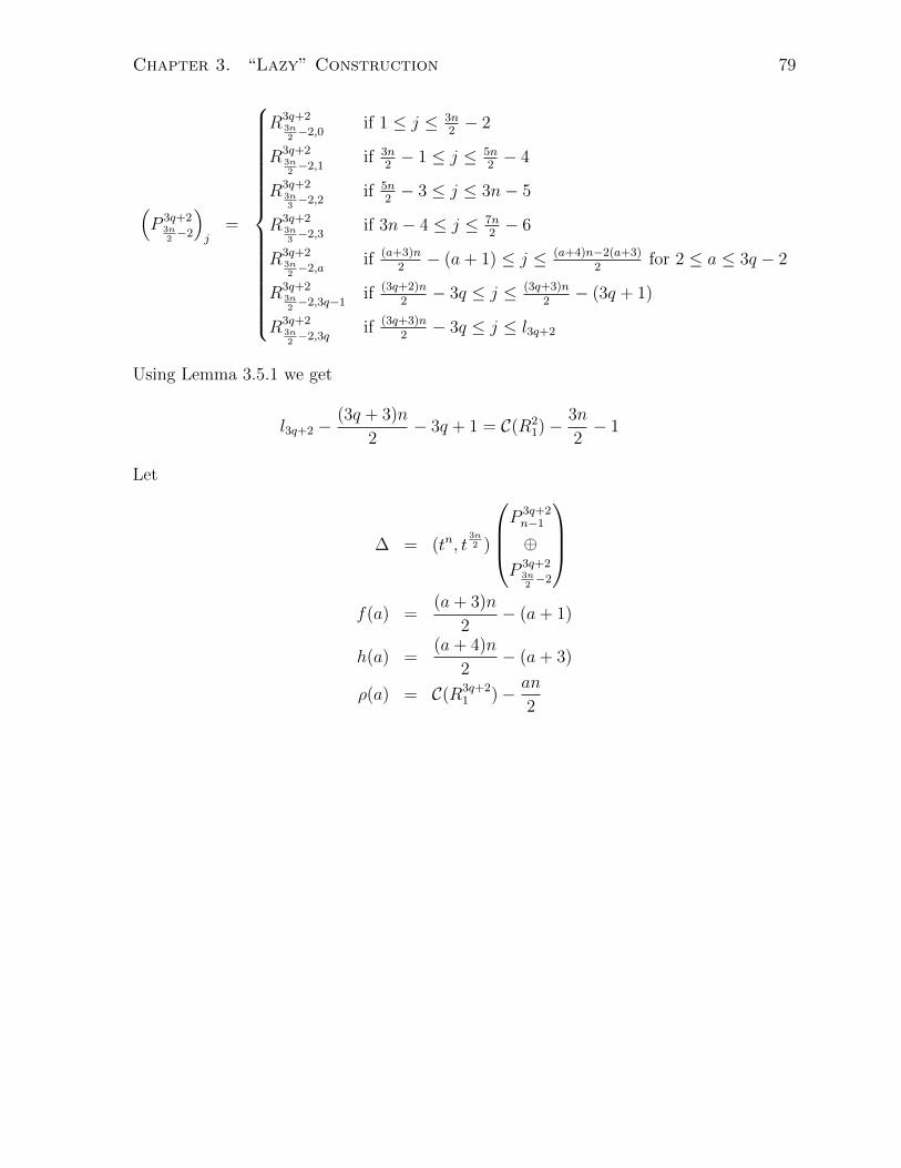
Chapter 3. “Lazy” Construction 79
(P 3q+2
3n2−2
)j
=
R3q+23n2−2,0 if 1 ≤ j ≤ 3n
2− 2
R3q+23n2−2,1 if 3n
2− 1 ≤ j ≤ 5n
2− 4
R3q+23n3−2,2 if 5n
2− 3 ≤ j ≤ 3n− 5
R3q+23n3−2,3 if 3n− 4 ≤ j ≤ 7n
2− 6
R3q+23n2−2,a if (a+3)n
2− (a+ 1) ≤ j ≤ (a+4)n−2(a+3)
2for 2 ≤ a ≤ 3q − 2
R3q+23n2−2,3q−1 if (3q+2)n
2− 3q ≤ j ≤ (3q+3)n
2− (3q + 1)
R3q+23n2−2,3q if (3q+3)n
2− 3q ≤ j ≤ l3q+2
Using Lemma 3.5.1 we get
l3q+2 −(3q + 3)n
2− 3q + 1 = C(R2
1)−3n
2− 1
Let
∆ = (tn, t3n2 )
P 3q+2n−1
⊕P 3q+2
3n2−2
f(a) =
(a+ 3)n
2− (a+ 1)
h(a) =(a+ 4)n
2− (a+ 3)
ρ(a) = C(R3q+21 )− an
2

Chapter 3. “Lazy” Construction 80
The image of (tn, t3n2 ) has the following presentation:
Value of j ∆j n 3n2
2n A3q+35 (n) C(R3q+2
1 ) · · ·1 ≤ j ≤ n− 1 tnR3q+2
n−1,0 x 0 x x x x
⊕t3n2 R3q+2
3n2−2,0 0 x 0 x x x
n ≤ j ≤ 3n2− 2 tnR3q+2
n−1,1 0 0 x x x x
⊕t3n2 R3q+2
3n2−2,0 0 x 0 x x x
3n2− 1 ≤ j ≤ 2n− 3 tnR3q+2
n−1,1 0 0 x x x x
⊕t3n2 R3q+2
3n2−2,1 0 0 0 x x x
2n− 2 ≤ j ≤ 5n2− 4 tnR3q+2
n−1,2 0 0 0 x x x
⊕t3n2 R3q+2
3n2−2,1 0 0 0 x x x
For 2 ≤ a ≤ 3q − 2 we have
Value of j ∆j A3q+3a+4 (n) C(R3q+2
1 ) · · ·f(a) ≤ j ≤ h(a) tnR3q+2
n−1,a+1 x x x
⊕t3n2 R3q+2
3n2−2,a x x x
and (note that h(3q − 2) + 1 = f(3q − 1))
Value of j ∆j(3q+3)n
2C(R3q+2
1 ) · · ·f(3q − 1) ≤ a ≤ h(3q − 2) + n
2tnR3q+2
n−1,3q x x x
⊕t3n2 R3q+2
3n2−2,3q−1 x x x
h(3q − 2) + n2
+ 1 ≤ a ≤ l3q+2 tnR3q+2n−1,3q+1 0 x x
⊕t3n2 R3q+2
3n2−2,3q 0 x x
In particular, Im(ζ) = J(P 3q+21 ) = ker π3q+2
1 . The kernel of ζ has the following presenta-
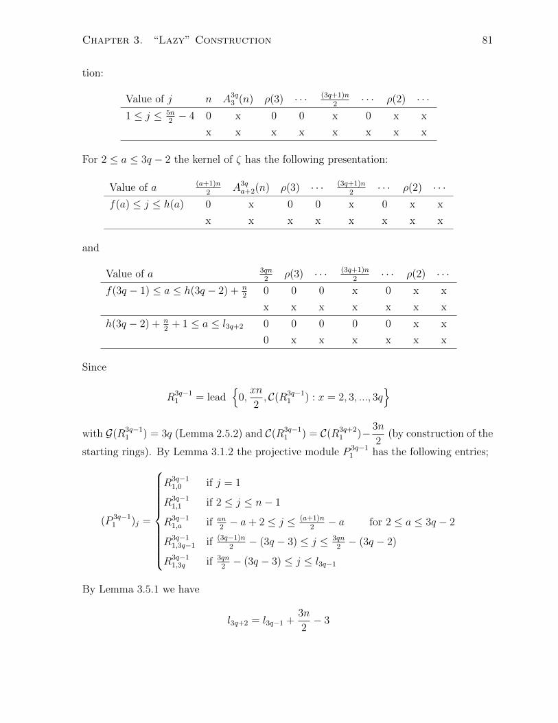
Chapter 3. “Lazy” Construction 81
tion:
Value of j n A3q3 (n) ρ(3) · · · (3q+1)n
2· · · ρ(2) · · ·
1 ≤ j ≤ 5n2− 4 0 x 0 0 x 0 x x
x x x x x x x x
For 2 ≤ a ≤ 3q − 2 the kernel of ζ has the following presentation:
Value of a (a+1)n2
A3qa+2(n) ρ(3) · · · (3q+1)n
2· · · ρ(2) · · ·
f(a) ≤ j ≤ h(a) 0 x 0 0 x 0 x x
x x x x x x x x
and
Value of a 3qn2
ρ(3) · · · (3q+1)n2
· · · ρ(2) · · ·f(3q − 1) ≤ a ≤ h(3q − 2) + n
20 0 0 x 0 x x
x x x x x x x
h(3q − 2) + n2
+ 1 ≤ a ≤ l3q+2 0 0 0 0 0 x x
0 x x x x x x
Since
R3q−11 = lead
{0,xn
2, C(R3q−1
1 ) : x = 2, 3, ..., 3q}
with G(R3q−11 ) = 3q (Lemma 2.5.2) and C(R3q−1
1 ) = C(R3q+21 )− 3n
2(by construction of the
starting rings). By Lemma 3.1.2 the projective module P 3q−11 has the following entries;
(P 3q−11 )j =
R3q−11,0 if j = 1
R3q−11,1 if 2 ≤ j ≤ n− 1
R3q−11,a if an
2− a+ 2 ≤ j ≤ (a+1)n
2− a for 2 ≤ a ≤ 3q − 2
R3q−11,3q−1 if (3q−1)n
2− (3q − 3) ≤ j ≤ 3qn
2− (3q − 2)
R3q−11,3q if 3qn
2− (3q − 3) ≤ j ≤ l3q−1
By Lemma 3.5.1 we have
l3q+2 = l3q−1 +3n
2− 3
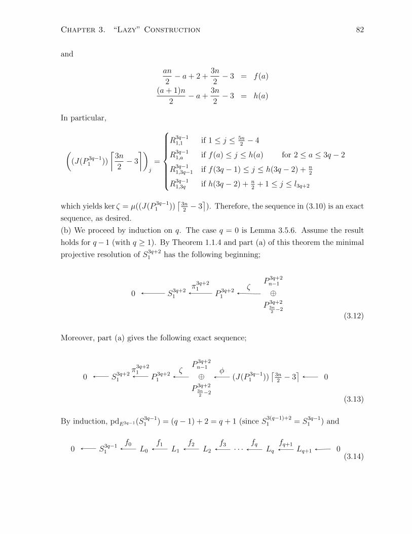
Chapter 3. “Lazy” Construction 82
and
an
2− a+ 2 +
3n
2− 3 = f(a)
(a+ 1)n
2− a+
3n
2− 3 = h(a)
In particular,
((J(P 3q−1
1 ))
⌈3n
2− 3
⌉)j
=
R3q−11,1 if 1 ≤ j ≤ 5n
2− 4
R3q−11,a if f(a) ≤ j ≤ h(a) for 2 ≤ a ≤ 3q − 2
R3q−11,3q−1 if f(3q − 1) ≤ j ≤ h(3q − 2) + n
2
R3q−11,3q if h(3q − 2) + n
2+ 1 ≤ j ≤ l3q+2
which yields ker ζ = µ((J(P 3q−11 ))
⌈3n2− 3⌉). Therefore, the sequence in (3.10) is an exact
sequence, as desired.
(b) We proceed by induction on q. The case q = 0 is Lemma 3.5.6. Assume the result
holds for q− 1 (with q ≥ 1). By Theorem 1.1.4 and part (a) of this theorem the minimal
projective resolution of S3q+21 has the following beginning;
0 S3q+21 P 3q+2
1
P 3q+2n−1
⊕P 3q+2
3n2−2
π3q+21 ζ
(3.12)
Moreover, part (a) gives the following exact sequence;
0 S3q+21 P 3q+2
1
P 3q+2n−1
⊕P 3q+2
3n2−2
(J(P 3q−11 ))
⌈3n2− 3⌉
0π3q+21 ζ φ
(3.13)
By induction, pdE3q−1(S3q−11 ) = (q − 1) + 2 = q + 1 (since S
3(q−1)+21 = S3q−1
1 ) and
0 S3q−11 L0 L1 L2 · · · Lq Lq+1 0
f0 f1 f2 f3 fq fq+1
(3.14)
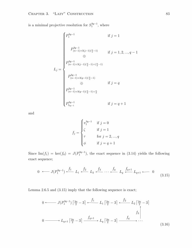
Chapter 3. “Lazy” Construction 83
is a minimal projective resolution for S3q−11 , where
Lj =
P 3q−11 if j = 1
P 3q−1(n−1)+3(j−1)(n
2−1)
⊕
P 3q−1(n−1)+3(j−1)(n
2−1)+(n
2−1)
if j = 1, 2, ..., q − 1
P 3q−1(n−1)+3(q−1)(n
2−1)
⊕
P 3q−1(n−1)+3(q−1)(n
2−1)+n
2
if j = q
P 3q−1l3q−1
if j = q + 1
and
fj =
π3q−11 if j = 0
ζ if j = 1
τ for j = 2, ..., q
φ if j = q + 1
Since Im(f1) = ker(f0) = J(P 3q−11 ), the exact sequence in (3.14) yields the following
exact sequence;
0 J(P 3q−11 ) L1 L2 · · · Lq Lq+1 0
f1 f2 f3 fq fq+1
(3.15)
Lemma 2.6.5 and (3.15) imply that the following sequence is exact;
0 J(P 3q−11 )
⌈3n2− 3⌉
L1
⌈3n2− 3⌉
L2
⌈3n2− 3⌉
0 Lq+1
⌈3n2− 3⌉
Lq⌈3n2− 3⌉
· · ·
f1 f2
f3fqfq+1
(3.16)

Chapter 3. “Lazy” Construction 84
Splicing (3.13) and (3.16) yields the following exact sequence;
0 S3q+21 P 3q+2
1
P 3q+2n−1
⊕P 3q+2
3n2−2
L1
⌈3n2− 3⌉
0 Lq+1
⌈3n2− 3⌉
Lq⌈3n2− 3⌉
· · · L2
⌈3n2− 3⌉
π3q+21 ζ τ = µζ
f2
fqfq+1 f3
(3.17)
Let
Wj =
P 3q+21 if j = 0
P 3q+2n−1 ⊕ P
3q+23n2−2 if j = 1
Lj−1[3n2− 3] if j = 2, ..., q + 2
and
dj =
π3q+21 if j = 0
ζ if j = 1
τ if j = 2
fj−1 if j = 3, ..., q + 2
In particular, (3.17) becomes the following exact sequence;
0 S3q+21 W0 W1 W2 · · · Wq+1 Wq+2 0
d0 d1 d2 d3 dq+1 dq+2
(3.18)
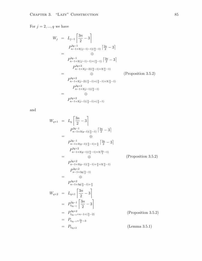
Chapter 3. “Lazy” Construction 85
For j = 2, ..., q we have
Wj = Lj−1
⌈3n
2− 3
⌉
=
P 3q−1n−1+3((j−1)−1)(n
2−1)⌈3n2− 3⌉
⊕P 3q−1n−1+3((j−1)−1)+(n
2−1)⌈3n2− 3⌉
=
P 3q+2n−1+3(j−2)(n
2−1)+3(n
2−1)
⊕P 3q+2n−1+3(j−2)(n
2−1)+(n
2−1)+3(n
2−1)
(Proposition 3.5.2)
=
P 3q+2n−1+3(j−1)(n
2−1)
⊕P 3q+2n−1+3(j−1)(n
2−1)+(n
2−1)
and
Wq+1 = Lq
⌈3n
2− 3
⌉
=
P 3q−1n−1+3(q−1)(n
2−1)⌈3n2− 3⌉
⊕P 3q−1n−1+3(q−1)(n
2−1)+n
2
⌈3n2− 3⌉
=
P 3q+2
n−1+3(q−1)(n2−1)+3( 3n
2−1)
⊕P 3q+2n−1+3(q−1)(n
2−1)+n
2+3(n
2−1)
(Proposition 3.5.2)
=
P 3q+2n−1+3q(n
2−1)
⊕P 3q+2n−1+3q(n
2−1)+n
2
Wq+2 = Lq+1
⌈3n
2− 3
⌉= P 3q−1
l3q−1
⌈3n
2− 3
⌉= P 3q+2
l3q−1+n−1+(n2−2) (Proposition 3.5.2)
= Pl3q−1+3n2−3
= Pl3q+2 (Lemma 3.5.1)

Chapter 3. “Lazy” Construction 86
That is, (3.18) is a projective resolution for S3q+21 . By Theorem 1.1.4
0 S3q+21 W0
d0
is a projective cover for S3q+21 . Since (3.12) is the start of the minimal projective resolution
for S3q+21 and (3.14) is the minimal projective resolution for S3q−1
1 , we have
Im(d1) = Im(ζ) = ker π3q+21 = J(P 3q+2
1 )
Im(d2) = Im(τ) = ker ζ ⊆ J(W1)
and for 3 ≤ j ≤ q + 2,
Im(Lj−1
fj−1−→ Lj−2
)⊆ J(Lj−2) by minimality of (3.14).
This implies that
Im(dj) = Im(fj−1)
⊆ J
(Lj−2
⌈3n
2− 3
⌉)(Lemma 2.6.6)
= J(Wj−1)
Thus, (3.18) is a minimal projective resolution for S3q+21 , as desired. The second part is
a consequence of what we just proved.
Notation 3.5.9. Let
η =
(tC(R
21)−(n/2)
−tC(R21)−n
), σ =
(t3n/2
−tn
), ε = C(R2
1)−3n
2
The following two theorems cover the cases when i is congruent to zero or 1.
Theorem 3.5.10. Let {Ri1|i ∈ N} be a set of starting rings constructed in section 2.5.
(a) The minimal projective resolution of S31 is as follows;
0 S31 P 3
1
P 3n−1
⊕P 3
3n2−2
P 3l3
0π31 ζ η

Chapter 3. “Lazy” Construction 87
In particular, pdE3(S31) = 2.
(b) If q ≥ 2, then
0 S3q1 P 3q
1
P 3qn−1
⊕P 3q
3n2−2
(J(P 3q−31 ))
⌈3n2− 3⌉
0π3q1 ζ µ
is an exact sequence, where
µ =
(tn2
−1
)
(c) If q ≥ 1, then
0 S3q1 W0 W1 W2 · · · Wq Wq+1 0
d0 d1 d2 d3 dq dq+1
is a minimal projective resolution for S3q1 , where
Wj =
P 3q1 if j = 0
P 3q(n−1)+3(j−1)(n
2−1)
⊕
P 3q(n−1)+3(j−1)(n
2−1)+(n
2−1)
if j = 1, 2, . . . , q
P 3ql3q
if j = q + 1
and
dj =
π3q1 if j = 0
ζ if j = 1
τ if j = 2, . . . , q
η if j = q + 1
In particular, pdE3q(S3q1 ) = q + 1 for q ∈ N⇒ gl. dim(E3q) ≥ q + 1 for q ∈ N.
Proof. The proof of part (a) is similar to the proof given in Lemma 3.5.6 and proofs of
parts (b) and (c) is similar to the proof given in Theorem 3.5.8.

Chapter 3. “Lazy” Construction 88
Theorem 3.5.11. Let {Ri1|i ∈ N} be a set of starting rings constructed in section 2.5.
(a) The minimal projective resolution of S11 and S4
1 are as follows;
0 S11 P 1
1 P 1n 0
π11 tn
0 S41 P 4
1
P 4n−1
⊕P 4
3n2−2
P 4l4−(ε−1) 0
π41 ζ σ
In particular, pdE1(S11) = 1 and pdE4(S4
1) = 2.
(b) If q ≥ 2, then
0 S3q+11 P 3q+1
1
P 3q+1n−1
⊕P 3q+1
3n2−2
(J(P 3q−21 ))
⌈3n2− 3⌉
0π3q+11 ζ µ
is an exact sequence, where
µ =
(tn/2
−1
)
(c) If q ≥ 1, then
0 S3q+11 W0 W1 W2 · · · Wq Wq+1 0
d0 d1 d2 d3 dq dq+1
is a minimal projective resolution for S3q+11 , where
Wj =
P 3q+11 if j = 0
P 3q+1(n−1)+3(j−1)(n
2−1)
⊕
P 3q+1(n−1)+3(j−1)(n
2−1)+(n
2−1)
if j = 1, 2, . . . , q
P 3q+1l3q+1−(ε−1) if j = q + 1

Chapter 3. “Lazy” Construction 89
and
dj =
π3q+11 if j = 0
ζ if j = 1
τ if j = 2, . . . , q
σ if j = q + 1
In particular, pdE3q+1(S3q+11 ) = q + 1 for q ∈ N0 ⇒ gl. dim(E3q+1) ≥ q + 1 for q ∈ N0.
Proof. The proof of part (a) is similar to the proof given in Lemmas 3.5.4 and 3.5.6, and
proofs of parts (b) and (c) is similar to the proof given in Theorem 3.5.8.
3.5.3 The Module M ′
Let
R1 ( R2 ( · · · ( Rl = k[[t]]
be an ascending chain of rings constructed via the lazy construction. We define
M ′ =l⊕
i=2
Ri and E ′ = EndR2(M′)
Since E is an l× l matrix, the matrix E ′ is (l−1)× (l−1) matrix. Furthermore, R1 ( R2
implies that EndR2(M′) = EndR1(M
′). The matrix E in block form has the following
form;
E =
(R1 (M ′)∗
HomR1(R1,M′) E ′
)
where
HomR1(R1,M′) = HomR1
(R1,
l⊕i=2
Ri
)=
l⊕i=2
HomR1(R1, Ri) =l⊕
i=2
Ri =
R2
R3
...
Rl
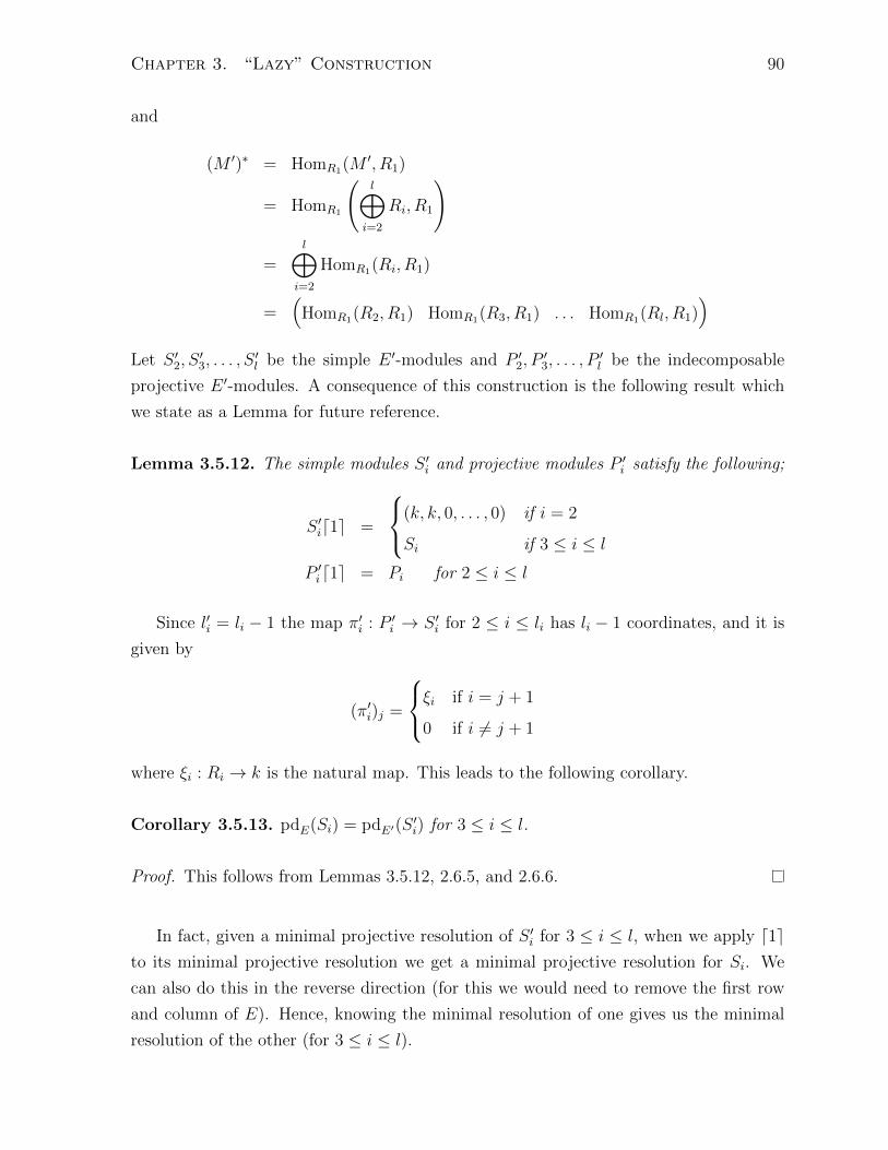
Chapter 3. “Lazy” Construction 90
and
(M ′)∗ = HomR1(M′, R1)
= HomR1
(l⊕
i=2
Ri, R1
)
=l⊕
i=2
HomR1(Ri, R1)
=(
HomR1(R2, R1) HomR1(R3, R1) . . . HomR1(Rl, R1))
Let S ′2, S′3, . . . , S
′l be the simple E ′-modules and P ′2, P
′3, . . . , P
′l be the indecomposable
projective E ′-modules. A consequence of this construction is the following result which
we state as a Lemma for future reference.
Lemma 3.5.12. The simple modules S ′i and projective modules P ′i satisfy the following;
S ′id1e =
(k, k, 0, . . . , 0) if i = 2
Si if 3 ≤ i ≤ l
P ′id1e = Pi for 2 ≤ i ≤ l
Since l′i = li − 1 the map π′i : P ′i → S ′i for 2 ≤ i ≤ li has li − 1 coordinates, and it is
given by
(π′i)j =
ξi if i = j + 1
0 if i 6= j + 1
where ξi : Ri → k is the natural map. This leads to the following corollary.
Corollary 3.5.13. pdE(Si) = pdE′(S′i) for 3 ≤ i ≤ l.
Proof. This follows from Lemmas 3.5.12, 2.6.5, and 2.6.6.
In fact, given a minimal projective resolution of S ′i for 3 ≤ i ≤ l, when we apply d1eto its minimal projective resolution we get a minimal projective resolution for Si. We
can also do this in the reverse direction (for this we would need to remove the first row
and column of E). Hence, knowing the minimal resolution of one gives us the minimal
resolution of the other (for 3 ≤ i ≤ l).

Chapter 3. “Lazy” Construction 91
3.5.4 Global Dimension
In this section we focus on computing the global dimension of Ei for a specific set of
starting rings. All the construction are via the lazy construction. To begin, we introduce
some notation.
Notation 3.5.14. Given positive inters a, b with a ≤ b, let
Vi(a, b) = max{pdEi(Sij) : j = a, a+ 1, ..., b}
Lemma 3.5.15. Suppose {Ri1 : i ∈ N} is a family of starting rings constructed in section
2.5. Then,
pdEi(Sij) = pdEi+1
(Si+1j+n
2−1
)for i ≥ 2, 2 ≤ j ≤ li. In particular,
Vi+1
(n2
+ 1, li+1
)= Vi(2, li)
for i ≥ 2.
Proof. Since Rij = Ri+1
j+n2−1 for i ≥ 2, 1 ≤ j ≤ li, we have
Sij
⌈n2− 1⌉
= Si+1j+n
2−1 for i ≥ 2, 2 ≤ j ≤ li (not true if j = 1)
P ij
⌈n2− 1⌉
= P i+1j+n
2−1 for i ≥ 2, 1 ≤ j ≤ li,
and li+1 = li +n
2− 1. In particular, given i ≥ 2 and 2 ≤ j ≤ li, if
0 Sij P ij W i
1 · · · W ia 0
πij f1 f2 fa
is a minimal projective resolution of Sij, then by Lemmas 2.6.5, 2.6.6 and Proposition

Chapter 3. “Lazy” Construction 92
3.5.2,
0 Sij⌈n2− 1⌉
P ij
⌈n2− 1⌉
W i1
⌈n2− 1⌉
0 W ia
⌈n2− 1⌉
· · ·
πij⌈n2− 1⌉
f1
f2
fa
is a minimal projective resolution of Sijdn2−1e = Si+1j+n
2−1. Hence,pdEi(Sij) = pdEi+1
(Si+1j+n
2−1
)for i ≥ 2, 2 ≤ j ≤ li. The second part is a consequence of what we just proved.
The matrix Ei+1 can be written as follows:
Ei+1 =
P i+11
P i+12
P i+13
···
P i+1n2−1
P i+1n2
P i+1n2+1
···
P i+1li+1
=
P i+11
P i+12
P i+13
···
P i+1n2−1
P i1
⌈n2− 1⌉
P i2
⌈n2− 1⌉
···
P ili
⌈n2− 1⌉
Lemma 3.5.16. Suppose {Ri
1 : i ∈ N} is a family of starting rings constructed in section
2.5, then
gl. dim(Ei+1) = max{Vi+1
(1,n
2
), Vi(2, li)
}for i ≥ 2
Proof. By Theorem 1.1.3 and Lemma 3.5.15,
gl. dim(Ei+1) = maxVi+1(1, li+1)
= max{Vi+1
(1,n
2
), Vi+1
(n2
+ 1, li+1
)}= max
{Vi+1
(1,n
2
), Vi(2, li)
}

Chapter 3. “Lazy” Construction 93
Lemma 3.5.17. Suppose n ≥ 6 is an even number and
R11 = lead
{0, n,
3n
2
},
then gl. dim(E1) = 2, V1(1, l1) = {1, 2} and V1(2, l1) = {2} where l1 =3n
2− 1.
Proof. This follows from Lemma 3.2.4 and its proof.
For the rest of this section
R11 = lead {0, 6, 9} := B1
1
Ri1 = lead {0, 3b, 11 + 3(i− 2) : b = 2, 3, ..., i+ 1} for i ≥ 2
Bi1 = lead {0, 3b, 12 + 3(i− 2) : b = 2, 3, ..., i+ 1} for i ≥ 2
Notice that these two sets of starting rings are of the type which was introduced in section
2.5 with n = 6, C(R21) = 11 and C(B2
1) = 12. We define
M i =
li⊕j=1
Rij and Ei = EndR1(M
i).
Lemma 3.5.18. gl. dim(E2) = 3 and V2(1, l2) = V2(2, l2) = {2, 3} where l2 = 9.
Proof. Notice that l2 = l1 + 1 = 9 and
S1j−1d1e = S2
j for 3 ≤ j ≤ l2
P 1j−1d1e = P 2
j for 2 ≤ j ≤ l2
Lemmas 2.6.5, 2.6.6, and 3.5.17 imply that pdE2(S2j ) = pdE1(S1
j−1) = 2 for 3 ≤ j ≤ 9.
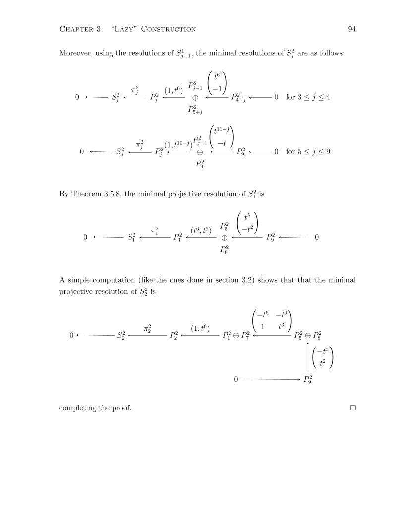
Chapter 3. “Lazy” Construction 94
Moreover, using the resolutions of S1j−1, the minimal resolutions of S2
j are as follows:
0 S2j P 2
j
P 2j−1
⊕P 25+j
P 24+j 0 for 3 ≤ j ≤ 4
π2j (1, t6)
(t6
−1
)
0 S2j P 2
j
P 2j−1
⊕P 29
P 29 0 for 5 ≤ j ≤ 9
π2j (1, t10−j)
(t11−j
−t
)
By Theorem 3.5.8, the minimal projective resolution of S21 is
0 S21 P 2
1
P 25
⊕P 28
P 29 0
π21 (t6, t9)
(t5
−t2
)
A simple computation (like the ones done in section 3.2) shows that that the minimal
projective resolution of S22 is
0 S22 P 2
2 P 21 ⊕ P 2
7 P 25 ⊕ P 2
8
0 P 29
π22 (1, t6)
(−t6 −t9
1 t3
)(−t5
t2
)
completing the proof.

Chapter 3. “Lazy” Construction 95
Notation 3.5.19. Let
1 = inclusion map
In is the n× n identity matrix
ζ = (t6, t9)
ϑ = (1, t3)
θ =
(t9
−t6
)
φ =
(t8
−t5
)
φ1 =
(t5
−t2
)
η =
(t6
−t3
)
τ =
(t9 t12
−t6 −t9
)
Lemma 3.5.20. gl. dim(E3) = 3 and V3(1, l3) = V3(2, l3) = {2, 3} where l3 = 11.
Proof. By Lemma 3.5.15, V3(4, 11) = V2(2, 9) = {2, 3}. By Theorem 3.5.10, the minimal
projective resolution of S31 is
0 S31 P 3
1
P 35
⊕P 37
P 311 0
π31 ζ φ
(3.19)
We now show pdE3(S32) = pdE3(S3
3) = 3, the proofs of which are given in great detail for
future reference. Using the definition introduced in section 3.5.3 we let
(M3)′ =
l3⊕j=2
R3j , (E3)′ = EndR3
2((M3)′) = EndR3
1((M3)′)
Since R32 = B2
1 , by Theorem 3.5.8 the minimal projective resolution of (S32)′ after renum-

Chapter 3. “Lazy” Construction 96
bering the subscripts is
0 (S32)′ (P 3
2 )′(P 3
6 )′
⊕(P 3
9 )′(P 3
11)′ 0
(π32)′ ζ η
(3.20)
where the above modules are (E3)′-modules. Applying d1e to the above exact sequence
makes the modules above into E3-modules, and Lemmas 2.6.5 and 2.6.6 yield the follow-
ing minimal projective resolution:
0 (S32)′d1e (P 3
2 )′d1e(P 3
6 )′d1e⊕
(P 39 )′d1e
(P 311)′d1e 0
(π32)′d1e ζ η
where
((π32)′d1e)j = 0 for 3 ≤ j ≤ l3,
and it is the natural map when j = 1, 2. More specifically,
0 (S32)′d1e P 3
2
P 36
⊕P 39
P 311 0
(π32)′d1e ζ η
(3.21)
is a minimal projective resolution. We can think of the sequences in (3.19) and (3.21)
as complexes by extending by zero’s on both sides. We have the following commutative

Chapter 3. “Lazy” Construction 97
diagram
0 S31 P 3
1
P 35
⊕P 37
P 311 0
0 (S32)′d1e P 3
2
P 36
⊕P 39
P 311 0
π31 ζ φ
(π32)′d1e ζ η
1 1 I2 t2
(3.22)
Taking the mapping cone gives us the following exact sequence (Lemma 1.5.1);
0
0
⊕(S3
2)′d1e
S31
⊕P 32
P 31
⊕P 36
⊕P 39
P 35
⊕P 37
⊕P 311
0
P 311
⊕0
(0 0
1 (π32)′d1e
) (−π3
1 0
1 ζ
) (−ζ 0
I2 η
)
(−φ 0
t2 0
)
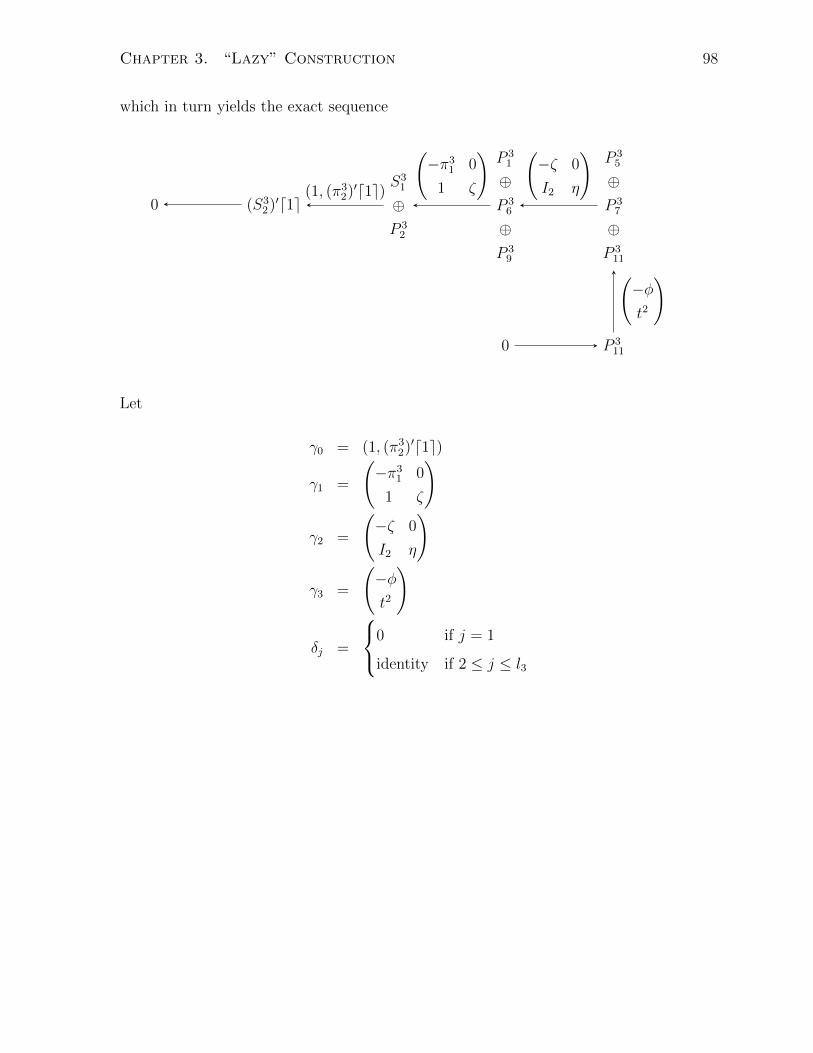
Chapter 3. “Lazy” Construction 98
which in turn yields the exact sequence
0 (S32)′d1e
S31
⊕P 32
P 31
⊕P 36
⊕P 39
P 35
⊕P 37
⊕P 311
0 P 311
(1, (π32)′d1e)
(−π3
1 0
1 ζ
) (−ζ 0
I2 η
)
(−φt2
)
Let
γ0 = (1, (π32)′d1e)
γ1 =
(−π3
1 0
1 ζ
)
γ2 =
(−ζ 0
I2 η
)
γ3 =
(−φt2
)
δj =
0 if j = 1
identity if 2 ≤ j ≤ l3
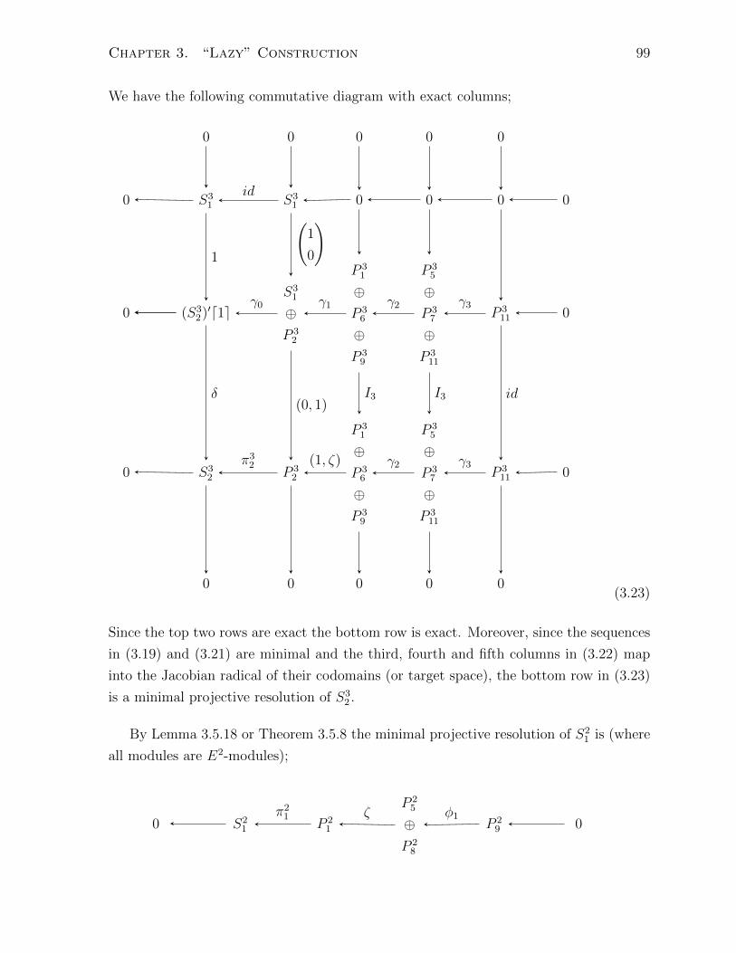
Chapter 3. “Lazy” Construction 99
We have the following commutative diagram with exact columns;
0 0 0 0 0
0 S31 S3
1 0 0 0 0
0 (S32)′d1e
S31
⊕P 32
P 31
⊕P 36
⊕P 39
P 35
⊕P 37
⊕P 311
P 311 0
0 S32 P 3
2
P 31
⊕P 36
⊕P 39
P 35
⊕P 37
⊕P 311
P 311 0
0 0 0 0 0
id
γ0 γ1 γ2 γ3
π32 (1, ζ) γ2 γ3
1
(1
0
)
(0, 1)δ I3 I3 id
(3.23)
Since the top two rows are exact the bottom row is exact. Moreover, since the sequences
in (3.19) and (3.21) are minimal and the third, fourth and fifth columns in (3.22) map
into the Jacobian radical of their codomains (or target space), the bottom row in (3.23)
is a minimal projective resolution of S32 .
By Lemma 3.5.18 or Theorem 3.5.8 the minimal projective resolution of S21 is (where
all modules are E2-modules);
0 S21 P 2
1
P 25
⊕P 28
P 29 0
π21 ζ φ1
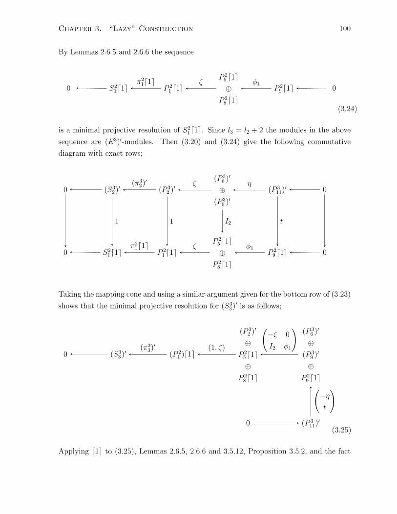
Chapter 3. “Lazy” Construction 100
By Lemmas 2.6.5 and 2.6.6 the sequence
0 S21d1e P 2
1 d1eP 25 d1e⊕
P 28 d1e
P 29 d1e 0
π21d1e ζ φ1
(3.24)
is a minimal projective resolution of S21d1e. Since l3 = l2 + 2 the modules in the above
sequence are (E3)′-modules. Then (3.20) and (3.24) give the following commutative
diagram with exact rows;
0 (S32)′ (P 3
2 )′(P 3
6 )′
⊕(P 3
9 )′(P 3
11)′ 0
0 S21d1e P 2
1 d1eP 25 d1e⊕
P 28 d1e
P 29 d1e 0
(π32)′ ζ η
π21d1e ζ φ1
1 1 I2 t
Taking the mapping cone and using a similar argument given for the bottom row of (3.23)
shows that the minimal projective resolution for (S33)′ is as follows;
0 (S33)′ (P 2
1 )d1e
(P 32 )′
⊕P 25 d1e⊕
P 28 d1e
(P 36 )′
⊕(P 3
9 )′
⊕P 29 d1e
0 (P 311)′
(π33)′ (1, ζ)
(−ζ 0
I2 φ1
)
(−ηt
)
(3.25)
Applying d1e to (3.25), Lemmas 2.6.5, 2.6.6 and 3.5.12, Proposition 3.5.2, and the fact

Chapter 3. “Lazy” Construction 101
that (π33)′d1e = π3
3 shows that
0 S33 P 3
3
P 32
⊕P 37
⊕P 310
P 36
⊕(P 3
9
⊕P 311
0 P 311
π33 (1, ζ)
(−ζ 0
I2 φ1
)
(−ηt
)
is the minimal projective resolution of S33 . Hence, gl. dim(E3) = 3 and V3(1, l3) =
V3(2, l3) = {2, 3}.
Lemma 3.5.21. gl. dim(E4) = 3 and V4(1, l4) = V4(2, l4) = {2, 3} where l4 = 13.
Proof. By Lemma 3.5.15, V4(4, 13) = V3(2, 11) = {2, 3}. A similar proof to the one given
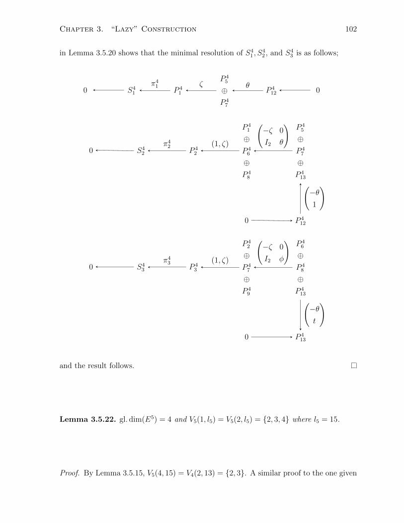
Chapter 3. “Lazy” Construction 102
in Lemma 3.5.20 shows that the minimal resolution of S41 , S
42 , and S4
3 is as follows;
0 S41 P 4
1
P 45
⊕P 47
P 412 0
π41 ζ θ
0 S42 P 4
2
P 41
⊕P 46
⊕P 48
P 45
⊕P 47
⊕P 413
0 P 412
π42 (1, ζ)
(−ζ 0
I2 θ
)
(−θ1
)
0 S43 P 4
3
P 42
⊕P 47
⊕P 49
P 46
⊕P 48
⊕P 413
0 P 413
π43 (1, ζ)
(−ζ 0
I2 φ
)
(−θt
)
and the result follows.
Lemma 3.5.22. gl. dim(E5) = 4 and V5(1, l5) = V5(2, l5) = {2, 3, 4} where l5 = 15.
Proof. By Lemma 3.5.15, V5(4, 15) = V4(2, 13) = {2, 3}. A similar proof to the one given
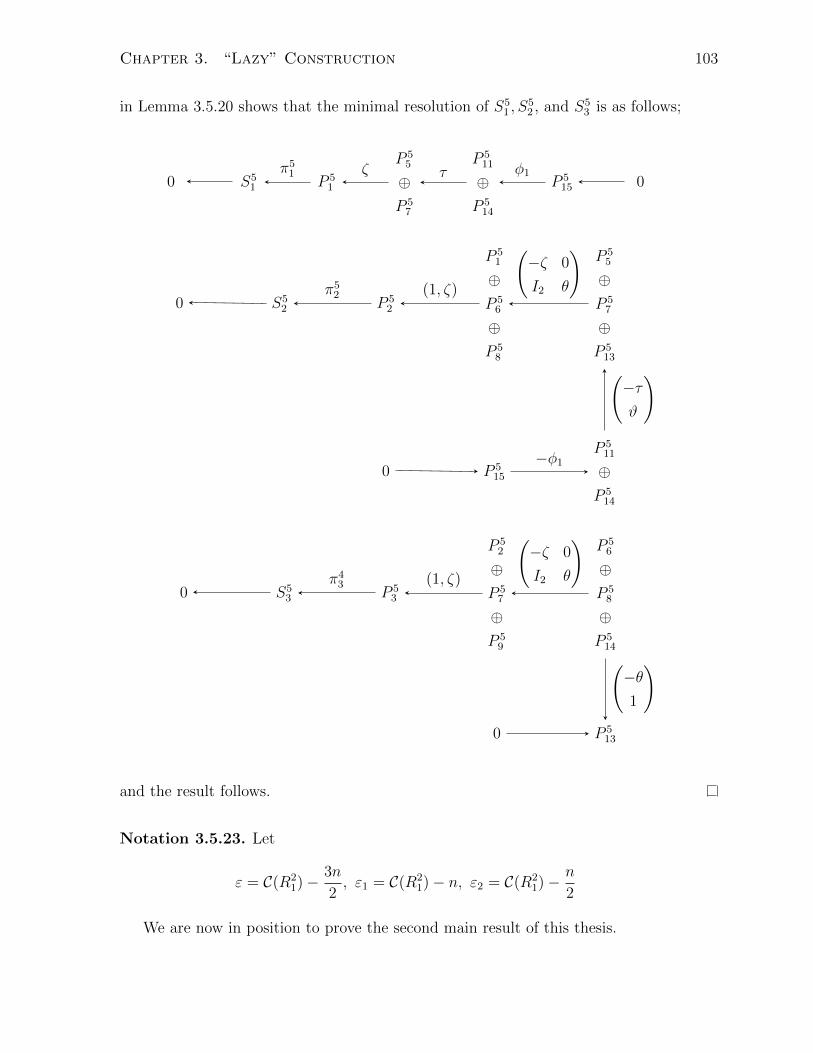
Chapter 3. “Lazy” Construction 103
in Lemma 3.5.20 shows that the minimal resolution of S51 , S
52 , and S5
3 is as follows;
0 S51 P 5
1
P 55
⊕P 57
P 511
⊕P 514
P 515 0
π51 ζ τ φ1
0 S52 P 5
2
P 51
⊕P 56
⊕P 58
P 55
⊕P 57
⊕P 513
0 P 515
P 511
⊕P 514
π52 (1, ζ)
(−ζ 0
I2 θ
)
(−τϑ
)
−φ1
0 S53 P 5
3
P 52
⊕P 57
⊕P 59
P 56
⊕P 58
⊕P 514
0 P 513
π43 (1, ζ)
(−ζ 0
I2 θ
)
(−θ1
)
and the result follows.
Notation 3.5.23. Let
ε = C(R21)−
3n
2, ε1 = C(R2
1)− n, ε2 = C(R21)−
n
2
We are now in position to prove the second main result of this thesis.

Chapter 3. “Lazy” Construction 104
Theorem 3.5.24. Let
R11 = lead {0, 6, 9}
Ri1 = lead {0, 3b, 11 + 3(i− 2) : b = 2, 3, ..., i+ 1} for i ≥ 2
where for each i the chain
Ri1 ( Ri
2 ( . . . ( Rili
= k[[t]],
the module M i and the ring Ei are constructed via the lazy construction. Then,
gl. dim(Ei) =
q + 2 if i = 3q or i = 3q + 1
q + 3 if i = 3q + 2,
V1(1, l1) = {1, 2}, V1(2, l1) = {2}, and Vi(1, li) = Vi(2, li) = {2, 3, . . . , gl. dim(Ei)} for
i ≥ 2.
Proof. We proceed by induction on i. The result holds for 1 ≤ i ≤ 5 by Lemmas 3.5.17,
3.5.18, 3.5.20, 3.5.21, and 3.5.22. Suppose the result holds for i where i ≥ 5. We consider
three cases.
Case 1. Suppose i = 3q + 1. By the induction hypothesis gl. dim(Ei) = q + 2 and
Vi+1(4, li+1) = Vi(2, li) = {2, 3, . . . , q + 2}
Since i+ 1 = 3q + 2 by Theorem 3.5.8 the minimal projective resolution of Si+11 is
H.D 0 1 . . . q q + 1 q + 2
0 Si+11 P i+1
1
P i+15
⊕P i+17
· · ·P i+16q−1
⊕P i+16q+1
P i+16q+5
⊕P i+16q+8
P i+1li+1
0πi+11 ζ τ τ τ φ1
That is, pdEi+1(Si+11 ) = q + 2. By Theorem 3.5.11 the minimal projective resolution of

Chapter 3. “Lazy” Construction 105
(Si+12 )′ (as an (Ei+1)′-module) is:
H.D 0 1 . . . q q + 1
0 (Si+12 )′ (P i+1
2 )′(P i+1
6 )′
⊕(P i+1
8 )′· · ·
(P i+16q )′
⊕(P i+1
6q+2)′
(P i+1li+1−2)
′ 0(πi+1
2 )′ ζ τ τ θ
(3.26)
Applying d1e to (3.26) and using a similar reasoning as done in the proof of Lemma
3.5.20 yields the following commutative diagram with exact rows (for convenience we
have removed the superscript i+ 1);
H.D −1 0 1 . . . q q + 1 q + 2
0 S1 P1
P5
⊕P7
· · ·P6q−1
⊕P6q+1
P6q+5
⊕P6q+8
Pli+10
0 S ′2[1] P2
P6
⊕P8
· · ·P6q
⊕P6q+2
Pli+1−2 0 0
π1 ζ τ τ τ φ1
π′2d1e ζ τ τ θ
δ−1 δ0 δ1 δqδq+1
δq+2
where
δ−1 = inclusion := 1
δ0 = inclusion := 1
δi = I2 for 1 ≤ i ≤ q
δq+1 = (1, t3)
δq+2 = 0

Chapter 3. “Lazy” Construction 106
Notice that
δ0(P1) ⊆ P2
δi
P6i−1
⊕P6i+1
⊆
J(P6i−1)
⊕J(P6i+2)
for 1 ≤ i ≤ q
δq+1
P6q+5
⊕P6q+8
⊆ J(Pli+1−2)
δq+2(Pli+1) = 0
The first through to the third inclusions follow from Lemma 2.4.1(b) and the fourth one
is obvious. Taking the mapping cone and using a similar argument as in the proof of

Chapter 3. “Lazy” Construction 107
Lemma 3.5.20 shows that the minimal projective resolution of Si+12 is as follows;
0 Si+12 P i+1
2
P i+11
⊕P i+16
⊕P i+18
P i+15
⊕P i+17
⊕P i+112
⊕P i+114
P i+16q−1
⊕P i+16q+1
⊕P i+1li+1−2
P i+16(q−1)−1
⊕P i+16(q−1)+1
⊕P i+16q
⊕P i+16q+2
. . .
P i+111
⊕P i+113
⊕P i+118
⊕P i+120
P i+16q+5
⊕P i+16q+8
P i+1li+1
0
πi+12 (1, ζ)
(−ζ 0
δ1 τ
)
(−τ 0
δ2 τ
)
(−τ 0
δq−1 τ
)(−τ 0
δq θ
)
(−τδq+1
)
−φ1
That is, pdEi+1(Si+12 ) = pdEi(Si+1
1 ) + 1 = q + 3.
By Theorem 3.5.11 the minimal projective resolution of Si1 is given by
H.D 0 1 . . . q q + 1
0 Si1 P i1
P i5
⊕P i7
· · ·P i5+6(q−1)
⊕P i7+6(q−1)
P ili−1 0
π1 ζ τ τ θ
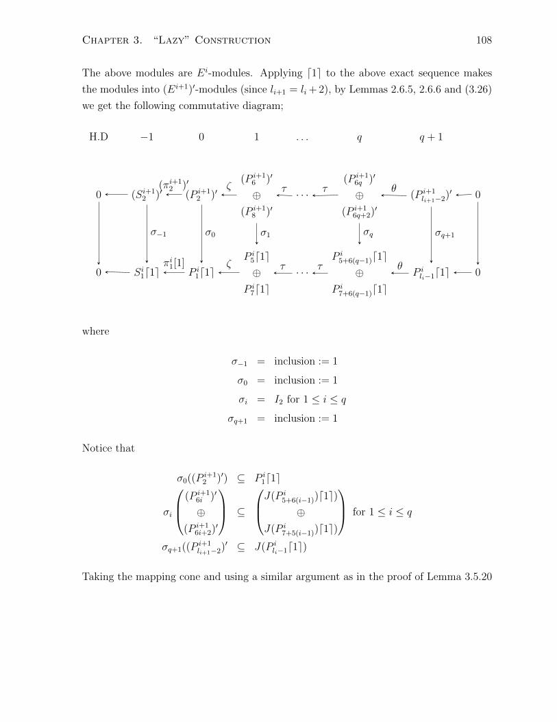
Chapter 3. “Lazy” Construction 108
The above modules are Ei-modules. Applying d1e to the above exact sequence makes
the modules into (Ei+1)′-modules (since li+1 = li + 2), by Lemmas 2.6.5, 2.6.6 and (3.26)
we get the following commutative diagram;
H.D −1 0 1 . . . q q + 1
0 (Si+12 )′ (P i+1
2 )′(P i+1
6 )′
⊕(P i+1
8 )′· · ·
(P i+16q )′
⊕(P i+1
6q+2)′
(P i+1li+1−2)
′ 0
0 Si1d1e P i1d1e
P i5d1e⊕
P i7d1e
· · ·P i5+6(q−1)d1e⊕
P i7+6(q−1)d1e
P ili−1d1e 0
(πi+12 )′ ζ τ τ θ
πi1[1] ζ τ τ θ
σ−1 σ0 σ1 σq σq+1
where
σ−1 = inclusion := 1
σ0 = inclusion := 1
σi = I2 for 1 ≤ i ≤ q
σq+1 = inclusion := 1
Notice that
σ0((Pi+12 )′) ⊆ P i
1d1e
σi
(P i+16i )′
⊕(P i+1
6i+2)′
⊆
J(P i5+6(i−1))d1e)⊕
J(P i7+5(i−1))d1e)
for 1 ≤ i ≤ q
σq+1((Pi+1li+1−2)
′ ⊆ J(P ili−1d1e)
Taking the mapping cone and using a similar argument as in the proof of Lemma 3.5.20
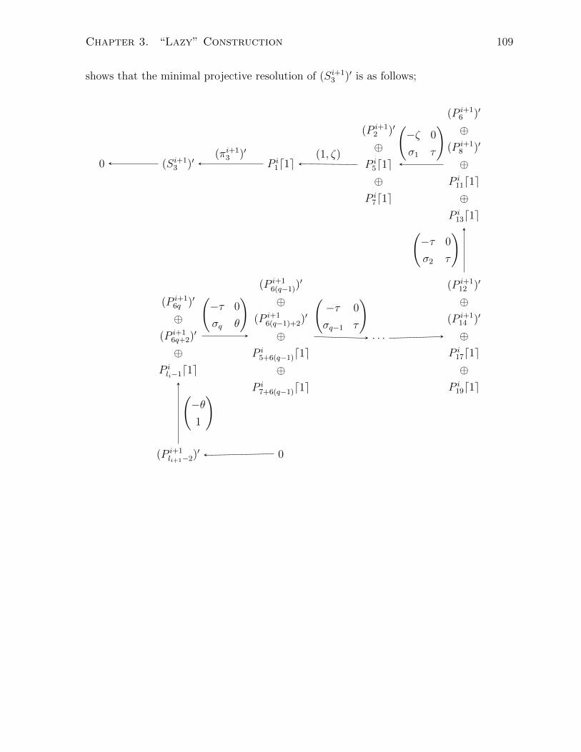
Chapter 3. “Lazy” Construction 109
shows that the minimal projective resolution of (Si+13 )′ is as follows;
0 (Si+13 )′ P i
1d1e
(P i+12 )′
⊕P i5d1e⊕
P i7d1e
(P i+16 )′
⊕(P i+1
8 )′
⊕P i11d1e⊕
P i13d1e
(P i+16q )′
⊕(P i+1
6q+2)′
⊕P ili−1d1e
(P i+16(q−1))
′
⊕(P i+1
6(q−1)+2)′
⊕P i5+6(q−1)d1e⊕
P i7+6(q−1)d1e
. . .
(P i+112 )′
⊕(P i+1
14 )′
⊕P i17d1e⊕
P i19d1e
(P i+1li+1−2)
′ 0
(πi+13 )′ (1, ζ)
(−ζ 0
σ1 τ
)
(−τ 0
σ2 τ
)
(−τ 0
σq−1 τ
)(−τ 0
σq θ
)
(−θ1
)

Chapter 3. “Lazy” Construction 110
Applying d1e gives us the minimal projective resolution of Si+13 ;
0 Si+13 P i+1
3
P i+12
⊕P i+17
⊕P i+19
P i+16
⊕P i+18
⊕P i+113
⊕P i+115
P i+16q
⊕P i+16q+2
⊕P ili+1−1
P i+16(q−1)
⊕P i+16(q−1)+2
⊕P i+17+6(q−1)
⊕P i+19+6(q−1)
. . .
P i+112
⊕P i+114
⊕P i+119
⊕P i+121
P i+1li+1−2 0
πi+13 (1, ζ)
(−ζ 0
σ1 τ
)
(−τ 0
σ2 τ
)
(−τ 0
σq−1 τ
)(−τ 0
σq θ
)
(−θ1
)
Hence, pdEi+1(Si+13 ) = q + 2, and the result follows.
Case 2. Suppose i = 3q. By the induction hypothesis gl. dim(Ei) = q + 2 and
Vi+1(4, li+1) = Vi(2, li) = {2, 3, . . . , q + 2}

Chapter 3. “Lazy” Construction 111
Since i+ 1 = 3q + 1 by Theorem 3.5.11 the minimal projective resolution of Si+11 is
H.D 0 1 . . . q q + 1
0 Si+11 P i+1
1
P i+15
⊕P i+17
· · ·P i+15+6(q−1)
⊕P i+17+6(q−1)
P i+1li+1−1 0
πi+11 ζ τ τ θ
That is, pdEi+1(Si+11 ) = q + 1. A similar argument as the one in case 1 shows that the
minimal projective resolution of Si+12 and Si+1
3 are as follows;
0 Si+12 P i+1
2
P i+11
⊕P i+16
⊕P i+18
P i+15
⊕P i+17
⊕P i+112
⊕P i+114
P i+15+6(q−1)
⊕P i+17+6(q−1)
⊕P i+1li+1
P i+15+6(q−2)
⊕P i+17+6(q−2)
⊕P i+16q
⊕P i+16q+2
. . .
P i+111
⊕P i+113
⊕P i+118
⊕P i+120
P i+1li+1−1 0
πi+12 (1, ζ)
(−ζ 0
I2 τ
)
(−τ 0
I2 τ
)
(−τ 0
I2 τ
)(−τ 0
I2 θ
)
(−θ1
)

Chapter 3. “Lazy” Construction 112
0 Si+13 P i+1
3
P i+12
⊕P i+17
⊕P i+19
P i+16
⊕P i+18
⊕P i+113
⊕P i+115
P i+16q
⊕P i+16q+2
⊕P ili+1
P i+16(q−1)
⊕P i+16(q−1)+2
⊕P i+17+6(q−1)
⊕P i+19+6(q−1)
. . .
P i+112
⊕P i+114
⊕P i+119
⊕P i+121
P i+1li+1
0
πi+13 (1, ζ)
(−ζ 0
I2 τ
)
(−τ 0
I2 τ
)
(−τ 0
I2 τ
)(−τ 0
I2 φ
)
(−θt
)
That is, pdEi+1(Si+12 ) = pdEi+1(Si+1
3 ) = q + 2 and the result follows.
Case 3. Suppose i = 3q + 2. By the induction hypothesis gl. dim(Ei) = q + 3 and
Vi+1(4, li+1) = Vi(2, li) = {2, 3, . . . , q + 3}
Since i + 1 = 3q + 3 = 3(q + 1) by Theorem 3.5.10 the minimal projective resolution of
Si+11 is
H.D 0 1 . . . q q + 1 q + 2
0 Si+11 P i+1
1
P i+15
⊕P i+17
· · ·P i+15+6(q−1)
⊕P i+17+6(q−1)
P i+15+6q
⊕P i+17+6q
P i+1li+1
0πi+11 ζ τ τ τ φ
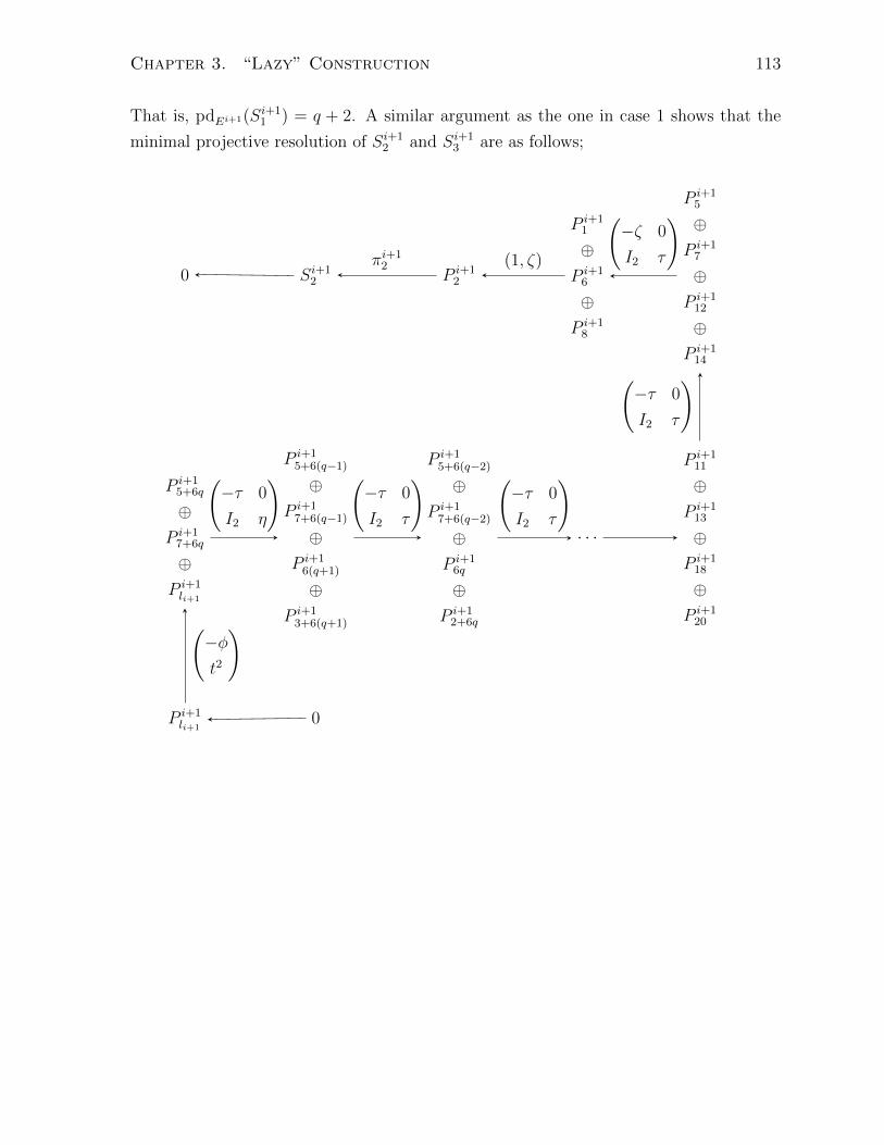
Chapter 3. “Lazy” Construction 113
That is, pdEi+1(Si+11 ) = q + 2. A similar argument as the one in case 1 shows that the
minimal projective resolution of Si+12 and Si+1
3 are as follows;
0 Si+12 P i+1
2
P i+11
⊕P i+16
⊕P i+18
P i+15
⊕P i+17
⊕P i+112
⊕P i+114
P i+15+6q
⊕P i+17+6q
⊕P i+1li+1
P i+15+6(q−1)
⊕P i+17+6(q−1)
⊕P i+16(q+1)
⊕P i+13+6(q+1)
P i+15+6(q−2)
⊕P i+17+6(q−2)
⊕P i+16q
⊕P i+12+6q
· · ·
P i+111
⊕P i+113
⊕P i+118
⊕P i+120
P i+1li+1
0
πi+12 (1, ζ)
(−ζ 0
I2 τ
)
(−τ 0
I2 τ
)
(−τ 0
I2 τ
)(−τ 0
I2 τ
)(−τ 0
I2 η
)
(−φt2
)
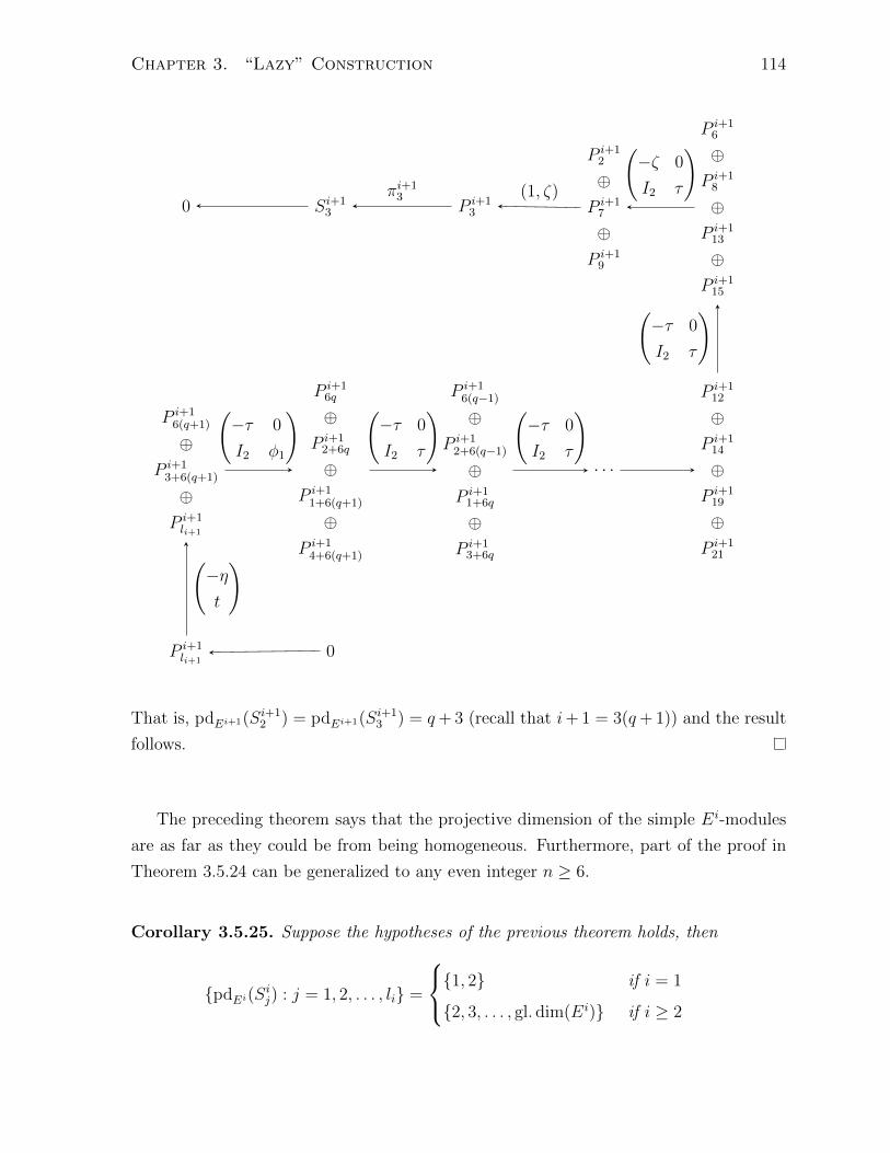
Chapter 3. “Lazy” Construction 114
0 Si+13 P i+1
3
P i+12
⊕P i+17
⊕P i+19
P i+16
⊕P i+18
⊕P i+113
⊕P i+115
P i+16(q+1)
⊕P i+13+6(q+1)
⊕P i+1li+1
P i+16q
⊕P i+12+6q
⊕P i+11+6(q+1)
⊕P i+14+6(q+1)
P i+16(q−1)
⊕P i+12+6(q−1)
⊕P i+11+6q
⊕P i+13+6q
· · ·
P i+112
⊕P i+114
⊕P i+119
⊕P i+121
P i+1li+1
0
πi+13 (1, ζ)
(−ζ 0
I2 τ
)
(−τ 0
I2 τ
)
(−τ 0
I2 τ
)(−τ 0
I2 τ
)(−τ 0
I2 φ1
)
(−ηt
)
That is, pdEi+1(Si+12 ) = pdEi+1(Si+1
3 ) = q+ 3 (recall that i+ 1 = 3(q+ 1)) and the result
follows.
The preceding theorem says that the projective dimension of the simple Ei-modules
are as far as they could be from being homogeneous. Furthermore, part of the proof in
Theorem 3.5.24 can be generalized to any even integer n ≥ 6.
Corollary 3.5.25. Suppose the hypotheses of the previous theorem holds, then
{pdEi(Sij) : j = 1, 2, . . . , li} =
{1, 2} if i = 1
{2, 3, . . . , gl. dim(Ei)} if i ≥ 2

Chapter 3. “Lazy” Construction 115
Corollary 3.5.26. Given an even integer n ≥ 6, let
R11 = lead
{0, n,
3n
2
}Ri
1 = lead
{0,bn
2,n(i+ 1)
2+ 2 : b = 2, 3, ..., i+ 1
}for i ≥ 2
where for each i the chain
Ri1 ( Ri
2 ( . . . ( Rili
= k[[t]],
the module M i and the ring Ei are constructed via the lazy construction. Then,
pdEi(Si2) = pdEi(Si1) + 1.
Proof. The proof in Theorem 3.5.24 shows this for n = 6. The value of n effects the
indices of the projective modules that appear in our projective resolutions, and when we
apply Lemma 3.5.15. However, the part of the proof to do with projective resolutions for
Si2 and Si3 only depends on ε = 2. Of course, for a given n, the indices of the projective
modules appearing in the minimal projective resolution of Si1 are given by Theorems
3.5.8, 3.5.10 and 3.5.11, and a similar argument in the proof of 3.5.24 gives the indices of
the projective modules that appear in the minimal projective resolution of Si2 and Si3.
Corollary 3.5.27. If ε = 2, then
pdE2(S2j ) =
3 if j = 2
2 if j 6= 2
In particular, gl. dim(E2) = 3.
Proof. Since ε = 2, R1j = R2
j+1 for 1 ≤ j ≤ l1 =3n
2− 1 and l2 = l1 + 1. More specifically,
P 1j d1e = P 2
j+1 for 1 ≤ j ≤ l1
S1j d1e = S2
j+1 for 2 ≤ j ≤ l1
Lemmas 2.6.5 and 2.6.6 imply that pdE2(S2j+1) = pdE1(S1
j ) for 2 ≤ j ≤ l1. By Lemma
3.2.4, pdE1(S1j ) = 2 for 2 ≤ j ≤ l1. By Theorem 3.5.8, pdE2(S2
1) = 2 and by Corollary
3.5.26, pdE2(S22) = 3.

Chapter 4
“Greedy” Construction
In this chapter we concentrate on a construction of our chain which minimizes its length,
called the “greedy” construction. More specifically, in section 4.1 we give the precise
definition of this construction. Section 4.2 focuses on computing the global dimension of
endomorphism rings for specific starting rings. In Section 4.3 we prove some of the results
which are a consequence of this construction. We conclude this chapter by proving the
third main theorem of this thesis.
4.1 The Construction
Given a ring of formal power series R1 6= k[[t]] associated to a numerical semigroup H,
define R2 = EndR1(m1) ) R1 (Theorem 1.1.1). If R2 = k[[t]], then stop. If not, let
R3 = EndR1(m2) ) R2 ) R1. If R3 = k[[t]], then stop. Otherwise, continue the process.
Since only finitely many positive powers of t are missing from R1, there exist a natural
number l such that Rl = k[[t]]. In particular,
Ri = EndR1(mi−1) for 2 ≤ i ≤ l
Since R1 is associated to a numerical semigroup, Ri are rings of formal power series. We
have constructed an ascending chain of rings;
R1 ( R2 ( ... ( Rl = k[[t]] (4.1)
Let
M :=
(l⊕
i=1
Ri
), E := EndR1(M)
116

Chapter 4. “Greedy” Construction 117
We say that the ascending chain (4.1), M and E are constructed via the ”greedy”.
Moreover, gl. dim(E) ≤ l by Proposition 2.2.2. This is the construction given in [11].
Example 4.1.1. Suppose R1 = lead {0, 5, 8}. Then,
R2 = EndR1(m1) = lead {0, 3}
R3 = EndR1(m2) = lead {0, 1} = k[[t]]
4.2 Special Rings II
In this section we compute the global dimension for some special starting rings. The
rings are analogous to the ones in section 3.2, however, the chains are constructed via
the greedy construction.
Lemma 4.2.1. Suppose
R1 = lead {0, n}
with n > 1. Then, gl. dim(E) = 2.
Proof. Notice that
R2 = EndR1(m1) = lead {0, 1} = k[[t]]
and
E =
(R1 tnR2
R2 R2
)
Since
(kerπ1)j = tnR2 for 1 ≤ j ≤ 2
= J(P1)
the minimal projective resolution for S1 is:
0 S1 P1 P2 0π1 tn
Also pdE(S2) = 2 by Proposition 2.4.3, the result follows by Theorem 1.1.3.
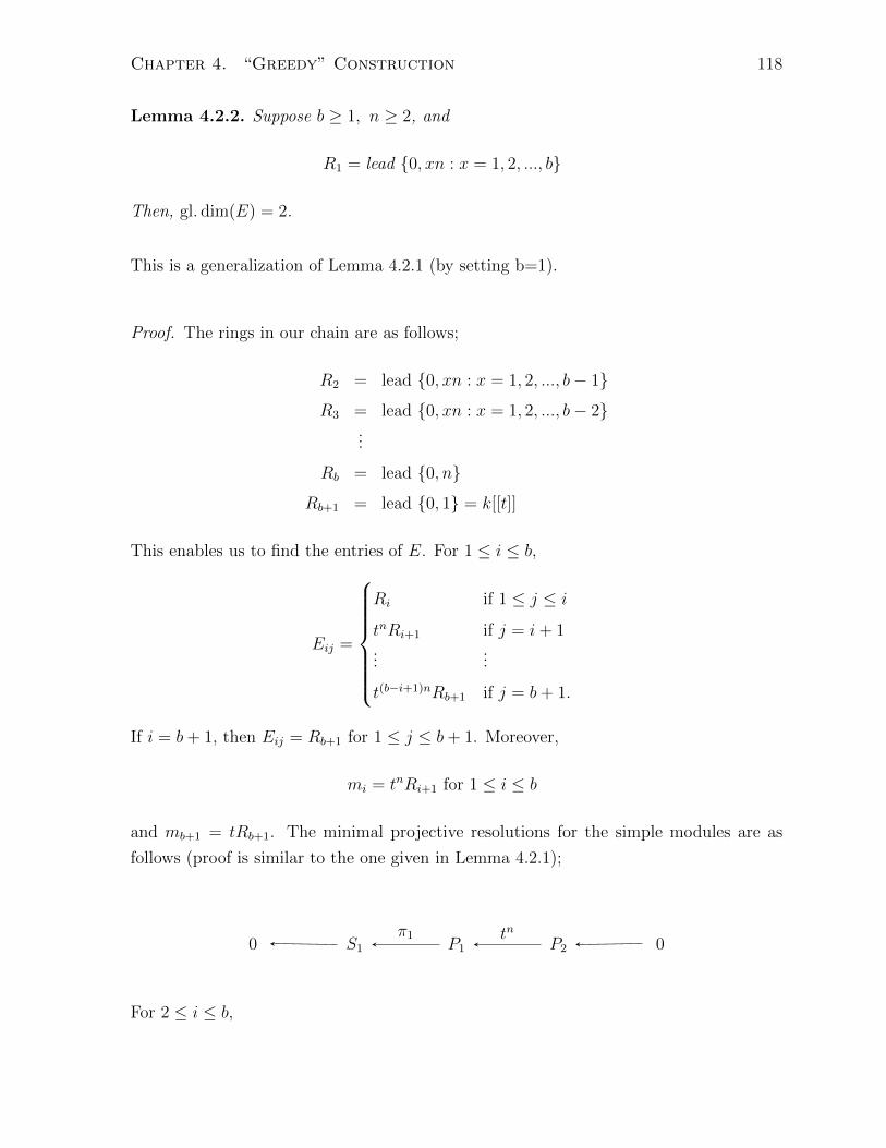
Chapter 4. “Greedy” Construction 118
Lemma 4.2.2. Suppose b ≥ 1, n ≥ 2, and
R1 = lead {0, xn : x = 1, 2, ..., b}
Then, gl. dim(E) = 2.
This is a generalization of Lemma 4.2.1 (by setting b=1).
Proof. The rings in our chain are as follows;
R2 = lead {0, xn : x = 1, 2, ..., b− 1}
R3 = lead {0, xn : x = 1, 2, ..., b− 2}...
Rb = lead {0, n}
Rb+1 = lead {0, 1} = k[[t]]
This enables us to find the entries of E. For 1 ≤ i ≤ b,
Eij =
Ri if 1 ≤ j ≤ i
tnRi+1 if j = i+ 1...
...
t(b−i+1)nRb+1 if j = b+ 1.
If i = b+ 1, then Eij = Rb+1 for 1 ≤ j ≤ b+ 1. Moreover,
mi = tnRi+1 for 1 ≤ i ≤ b
and mb+1 = tRb+1. The minimal projective resolutions for the simple modules are as
follows (proof is similar to the one given in Lemma 4.2.1);
0 S1 P1 P2 0π1 tn
For 2 ≤ i ≤ b,

Chapter 4. “Greedy” Construction 119
0 Si Pi
Pi−1
⊕Pi+1
Pi 0πi (1, tn)
(tn
−1
)
and
0 Sb+1 Pb+1
Pb
⊕Pb+1
Pb+1 0πb+1 (1, t)
(tn
−tn−1
)
The result follows by Theorem 1.1.3.
Example 4.2.3. Let b = n = 3, then
R1 = lead {0, 3, 6, 9}
R2 = lead {0, 3, 6}
R3 = lead {0, 3}
R4 = lead {0, 1}
and
E =
R1 t3R2 t6R3 t9R4
R2 R2 t3R3 t6R4
R3 R3 R3 t3R4
R4 R4 R4 R4
,
The minimal projective resolutions of the simple modules are as follows;
0 S1 P1 P2 0π1 t3
0 S2 P2
P1
⊕P3
P2 0π2 (1, t3)
(t3
−1
)
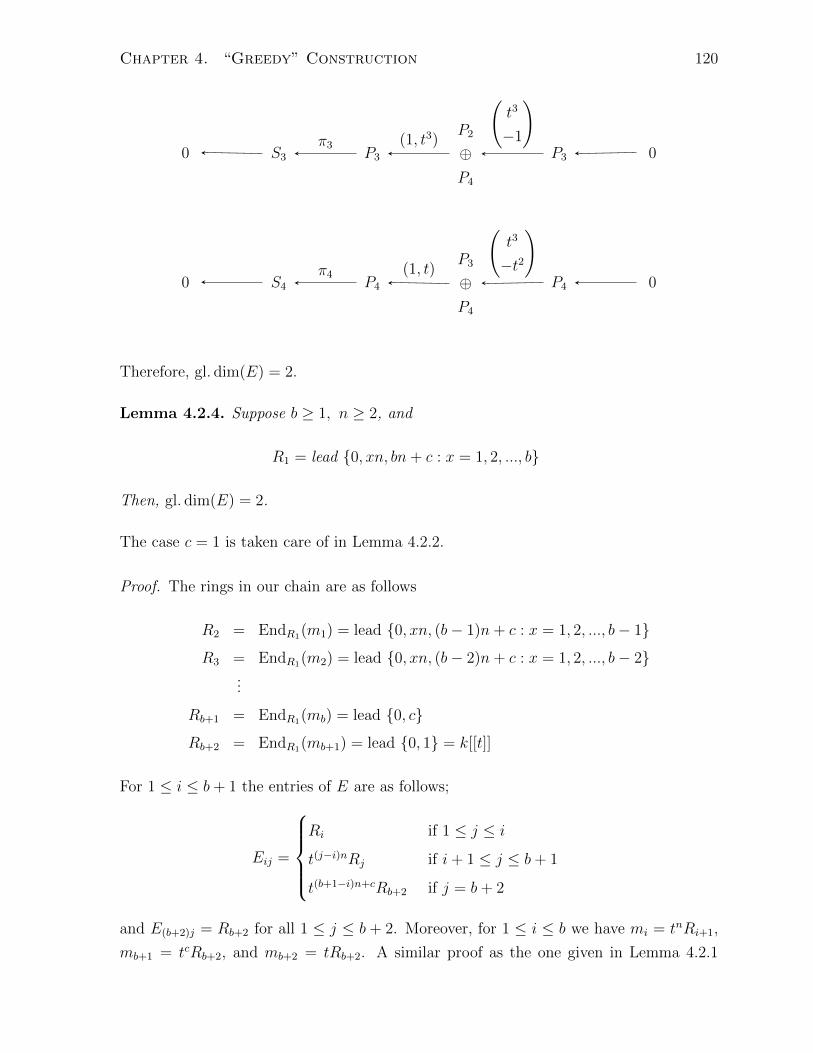
Chapter 4. “Greedy” Construction 120
0 S3 P3
P2
⊕P4
P3 0π3 (1, t3)
(t3
−1
)
0 S4 P4
P3
⊕P4
P4 0π4 (1, t)
(t3
−t2
)
Therefore, gl. dim(E) = 2.
Lemma 4.2.4. Suppose b ≥ 1, n ≥ 2, and
R1 = lead {0, xn, bn+ c : x = 1, 2, ..., b}
Then, gl. dim(E) = 2.
The case c = 1 is taken care of in Lemma 4.2.2.
Proof. The rings in our chain are as follows
R2 = EndR1(m1) = lead {0, xn, (b− 1)n+ c : x = 1, 2, ..., b− 1}
R3 = EndR1(m2) = lead {0, xn, (b− 2)n+ c : x = 1, 2, ..., b− 2}...
Rb+1 = EndR1(mb) = lead {0, c}
Rb+2 = EndR1(mb+1) = lead {0, 1} = k[[t]]
For 1 ≤ i ≤ b+ 1 the entries of E are as follows;
Eij =
Ri if 1 ≤ j ≤ i
t(j−i)nRj if i+ 1 ≤ j ≤ b+ 1
t(b+1−i)n+cRb+2 if j = b+ 2
and E(b+2)j = Rb+2 for all 1 ≤ j ≤ b + 2. Moreover, for 1 ≤ i ≤ b we have mi = tnRi+1,
mb+1 = tcRb+2, and mb+2 = tRb+2. A similar proof as the one given in Lemma 4.2.1
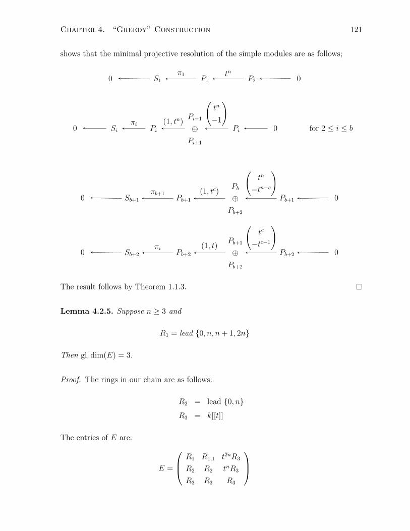
Chapter 4. “Greedy” Construction 121
shows that the minimal projective resolution of the simple modules are as follows;
0 S1 P1 P2 0π1 tn
0 Si Pi
Pi−1
⊕Pi+1
Pi 0 for 2 ≤ i ≤ bπi (1, tn)
(tn
−1
)
0 Sb+1 Pb+1
Pb
⊕Pb+2
Pb+1 0πb+1 (1, tc)
(tn
−tn−c
)
0 Sb+2 Pb+2
Pb+1
⊕Pb+2
Pb+2 0πi (1, t)
(tc
−tc−1
)
The result follows by Theorem 1.1.3.
Lemma 4.2.5. Suppose n ≥ 3 and
R1 = lead {0, n, n+ 1, 2n}
Then gl. dim(E) = 3.
Proof. The rings in our chain are as follows:
R2 = lead {0, n}
R3 = k[[t]]
The entries of E are:
E =
R1 R1,1 t2nR3
R2 R2 tnR3
R3 R3 R3

Chapter 4. “Greedy” Construction 122
Let
∆ = (tn, tn+1)
P2
⊕P2
The image of (tn, tn+1) has the following presentation:
Value of j ∆j n n+ 1 . . . 2n . . .
j = 1, 2 tnR2 x 0 0 x x
⊕tn+1R2 0 x 0 0 x
j = 3 tn(tnR3) 0 0 0 x x
⊕tn+1(tnR3) 0 0 0 0 x
That is, Im(tn, tn+1) = ker π1 = J(P1). The kernel of (tn, tn+1) has the following presen-
tation:
Value of j n n+ 1 . . .
1 ≤ j ≤ 3 0 x x
x x x
That is,
ker(tn, tn+1) =
(tn+1
−tn
)P3 ( J
P2
⊕P2
Thus, the minimal projective resolution for S1 is
0 S1 P1
P2
⊕P2
P3 0π1 (tn, tn+1)
(tn+1
−tn
)
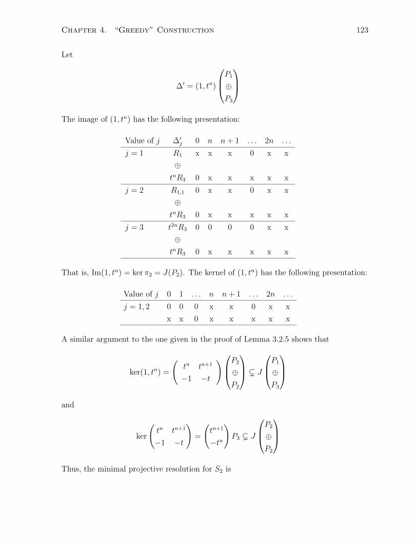
Chapter 4. “Greedy” Construction 123
Let
∆′ = (1, tn)
P1
⊕P3
The image of (1, tn) has the following presentation:
Value of j ∆′j 0 n n+ 1 . . . 2n . . .
j = 1 R1 x x x 0 x x
⊕tnR3 0 x x x x x
j = 2 R1,1 0 x x 0 x x
⊕tnR3 0 x x x x x
j = 3 t2nR3 0 0 0 0 x x
⊕tnR3 0 x x x x x
That is, Im(1, tn) = ker π2 = J(P2). The kernel of (1, tn) has the following presentation:
Value of j 0 1 . . . n n+ 1 . . . 2n . . .
j = 1, 2 0 0 0 x x 0 x x
x x 0 x x x x x
A similar argument to the one given in the proof of Lemma 3.2.5 shows that
ker(1, tn) =
(tn tn+1
−1 −t
)P2
⊕P2
( J
P1
⊕P3
and
ker
(tn tn+1
−1 −t
)=
(tn+1
−tn
)P3 ( J
P2
⊕P2
Thus, the minimal projective resolution for S2 is

Chapter 4. “Greedy” Construction 124
0 S2 P2
P1
⊕P3
P2
⊕P2
P3 0π2 (1, tn)
(tn tn+1
−1 −t
) (tn+1
−tn
)
By Proposition 2.4.3 we have pdE(S3) = 2, and the result follows by Theorem 1.1.3.
Lemma 4.2.6. Suppose n ≥ 3 and
R1 = lead {0, n, n+ 1, n+ 3}
Then, gl. dim(E) = 3.
Proof. The rings in our chain are as follows;
R2 = lead {0, 3}
R3 = lead {0, 1} = k[[t]]
and
E =
R1 m1 tn+3R3
R2 R2 t3R3
R3 R3 R3
A similar argument to the one given in the proof of Lemma 4.2.5 shows that the minimal
projective resolutions of the simple modules are as follows;
0 S1 P1
P2
⊕P2
P3 0π1 (tn, tn+1)
(t4
−t3
)

Chapter 4. “Greedy” Construction 125
0 S2 P2
P1
⊕P3
P2
⊕P2
0 P3
π2 (1, t3)
(tn tn+1
−tn−3 −tn−2
)
(t4
−t3
)
0 S3 P3
P2
⊕P3
P3 0π3 (1, t)
(t3
−t2
)
The result follows by Theorem 1.1.3.
4.3 Minor Results III
In this section we concentrate on some of the results that follow when our chain
R1 ( R2 ( ... ( Rl = k[[t]]
is constructed via the greedy construction.
Lemma 4.3.1. (a) If e(Ri) = C(Ri) then i = l − 1 or i = l.
(b) If e(Ri) < C(Ri) then C(Ri+1) = C(Ri)− e(Ri).
Proof. (a) If i = l, nothing to prove. If i < l, then e(Ri) = C(Ri) > 1. This implies
that Ri = lead{0, e(Ri)}. In particular, Ri+1 = EndR1(mi) = lead{0, 1} = k[[t]]. Hence,
i+ 1 = l, as desired.
(b) Let Γ(Ri) = {β1, β2, · · · , βr}, where e(Ri) = β1 < β2 < · · · < βr = C(Ri) (notice
that r ≥ 2). Then, tx ∈ Ri+1 = EndR1(mi) for all x ≥ βr − β1, which implies that
C(Ri+1) ≤ C(Ri) − e(Ri). However, tβr−β1−1 /∈ Ri+1. To see this, if tβr−β1−1 ∈ Ri+1,
then tβr−1 = tβ1tβr−β1−1 ∈ mi ⊆ Ri, a contradiction. Hence, C(Ri+1) ≥ C(Ri) − e(Ri),
completing the proof.
If l = 1, that is, R1 = k[[t]], then Proposition 1.1.2 implies that gl. dim(E) = 1.
Meanwhile, if l = 2 then Lemma 4.2.1 yields gl. dim(E) = 2.

Chapter 4. “Greedy” Construction 126
Lemma 4.3.2. If l = 3, then gl. dim(E) = 2 or 3.
Proof. This follows from Lemmas 4.2.2, 4.2.4, 4.2.5, 4.2.6 and Propositions 2.2.2, 2.3.6.
Lemma 2.2.17 gives us l ≤ g(R1) + 1, however, under the greedy construction this
upper bound is usually too large.
Conjecture 2. l ≤ G(R1) + 1.
The following two examples illustrate that the inequality can be an equality or strict.
Example 4.3.3. Suppose R1 = lead {0, 10, 20, 30}. Then G(R1) = 3, and
R2 = lead {0, 10, 20}
R3 = lead {0, 10}
R4 = lead {0, 1} = k[[t]]
That is, l = G(R1) + 1.
Example 4.3.4. Suppose R1 = lead {0, 10, 16, 20, 22, 24, 26, 30}. Then G(R1) = 7,
however,
R2 = lead {0, 10, 14, 16, 20}
R3 = lead {0, 6, 10}
R4 = lead {0, 4}
R5 = lead {0, 1} = k[[t]]
That is, l < G(R1) + 1.
This construction is more erratic then the lazy construction. One of the main problems
that arises is the erratic behaviour of the multiplicity of Ri in our chain. The following
examples show how some of the results that hold under the lazy construction fail under
the greedy construction.
Example 4.3.5. If R1 = lead {0, 7, 10, 13}, then R2 = lead {0, 3, 6}. That is,
e(R2) = 3 < 7 = e(R1) but G(R2) = 2.
In particular, Lemma 3.3.1 does not hold for the greedy construction.

Chapter 4. “Greedy” Construction 127
Example 4.3.6. Let
R1 = lead{0, 3, 6, 7, 9}
R2 = EndR1(m1) = lead{0, 3, 4, 6}
R3 = EndR1(m2) = lead{0, 3}
R4 = EndR1(m3) = lead{0, 1}
Then
E =
R1,0 R1,1 R1,2 R1,4
R2,0 R2,0 R2,1 R2,3
R3,0 R3,0 R3,0 R3,1
R4,0 R4,0 R4,0 R4,0
=
P1
P2
P3
P4
A simple calculation shows that the minimal projective resolution of the simple modules

Chapter 4. “Greedy” Construction 128
are as follows;
0 S1 P1 P2 0π1 t3
0 S2 P2
P1
⊕P3
⊕P3
P2
⊕P4
0π2 (1, t3, t4)
−t3 0
1 −t4
0 t3
0 S3 P3
P2
⊕P4
P3
⊕P3
0 P4
π3 (1, t3)
(t3 t4
−1 −t
)
(t4
−t3
)
0 S4 P4
P3
⊕P4
P4 0π4 (1, t)
(t3
−t2
)
In particular, gl. dim(E) = 3. This shows that Proposition 3.3.2 fails under the greedy
construction.
4.4 gl. dim(Ei) = 2
Throughout this section {Ri1| i ∈ N} is the set of starting rings constructed in section
2.5 with M i and Ei constructed via the ”greedy” construction. The third main result of
this thesis is that gl. dim(Ei) = 2 for all i ∈ N (Theorem 4.4.7). In particular, when the
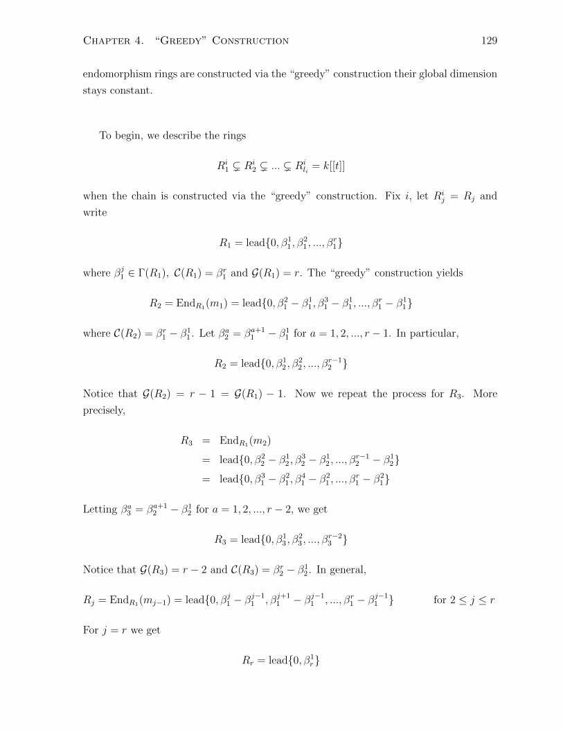
Chapter 4. “Greedy” Construction 129
endomorphism rings are constructed via the “greedy” construction their global dimension
stays constant.
To begin, we describe the rings
Ri1 ( Ri
2 ( ... ( Rili
= k[[t]]
when the chain is constructed via the “greedy” construction. Fix i, let Rij = Rj and
write
R1 = lead{0, β11 , β
21 , ..., β
r1}
where βj1 ∈ Γ(R1), C(R1) = βr1 and G(R1) = r. The “greedy” construction yields
R2 = EndR1(m1) = lead{0, β21 − β1
1 , β31 − β1
1 , ..., βr1 − β1
1}
where C(R2) = βr1 − β11 . Let βa2 = βa+1
1 − β11 for a = 1, 2, ..., r − 1. In particular,
R2 = lead{0, β12 , β
22 , ..., β
r−12 }
Notice that G(R2) = r − 1 = G(R1) − 1. Now we repeat the process for R3. More
precisely,
R3 = EndR1(m2)
= lead{0, β22 − β1
2 , β32 − β1
2 , ..., βr−12 − β1
2}
= lead{0, β31 − β2
1 , β41 − β2
1 , ..., βr1 − β2
1}
Letting βa3 = βa+12 − β1
2 for a = 1, 2, ..., r − 2, we get
R3 = lead{0, β13 , β
23 , ..., β
r−23 }
Notice that G(R3) = r − 2 and C(R3) = βr2 − β12 . In general,
Rj = EndR1(mj−1) = lead{0, βj1 − βj−11 , βj+1
1 − βj−11 , ..., βr1 − βj−11 } for 2 ≤ j ≤ r
For j = r we get
Rr = lead{0, β1r}

Chapter 4. “Greedy” Construction 130
where β1r = βr1 − βr−11 . Notice that Rr+1 = k[[t]] = lead{0, 1}. This proves the following
lemma.
Lemma 4.4.1. For each i ∈ N the following hold;
(a) li = G(Ri1) + 1 = i+ 2. Moreover, G(Ri
j+1) = G(Rij)− 1 for j = 1, 2, ..., li − 1
(b) As a matrix, the entries of Ei are as follows;
(P ij )a = Ei
ja =
Rij,0 if 1 ≤ a ≤ j
Rij,a−j if j + 1 ≤ a ≤ li
(c) For a fixed i,
Rij,a = te(R
ij)Ri
j+1,a−1 for 1 ≤ a ≤ G(Rij)
(d) For a fixed i,
R11 = lead
{0, n,
3n
2
}Ri
1 = lead
{0, n,
3n
2, ...,
(i+ 1)n
2, C(Ri
1)
}for i ≥ 2
Rij = lead
{0,n
2, n, ...,
(i− j + 1)n
2, C(Ri
1)−jn
2
}for 2 ≤ j ≤ li − 2
Rili−1 = lead
{0, C(R2
1)−3n
2
}Rili
= k[[t]]
(e) For i ≥ 3 and 3 ≤ j ≤ li we have Rij = Ri−1
j−1. In particular,
P i−1j−1d1e = P i
j and (J(P i−1j−1))d1e = J(P i
j )
Part (d) of the previous proposition tells us e(Ri1) = n for all i ∈ N. The next
proposition gives us the minimal projective resolution of the first simple module.
Lemma 4.4.2. The minimal projective resolution of Si1 is:
0 Si1 P i1 P i
2 0πi1 tn
In particular, pdEi(Si1) = 1 for all i ∈ N.

Chapter 4. “Greedy” Construction 131
Proof. By Proposition 4.4.1 (b)
(P i1)a = Ri
1,a−1 for 1 ≤ a ≤ G(Ri1) + 1
In particular,
(kerπi1)a = (J(P i1))a =
Ri1,1 if a = 1, 2
Ri1,a−1 if 3 ≤ a ≤ G(Ri
1) + 1
=
te(Ri1)Ri
2,0 if a = 1, 2
te(Ri1)Ri
2,a−2 if 3 ≤ a ≤ G(Ri1) + 1
(Lemma 4.4.1(c))
=
tnRi2,0 if a = 1, 2
tnRi2,a−2 if 3 ≤ a ≤ G(Ri
1) + 1
and the result follows.
The following results use the notations introduced in section 3.5.4.
Lemma 4.4.3. gl. dim(E1) = gl. dim(E2) = 2.
Proof. Since R11 = lead
{0, n,
3n
2
}, the greedy construction yields
R12 = lead
{0,n
2
}R1
3 = lead{0, 1} = k[[t]]
In particular,
E1 = EndR11(R1
1 ⊕R12 ⊕R1
3) =
R11,0 R1
1,1 R11,2
R12,0 R1
2,0 R12,1
R13,0 R1
3,0 R13,0
By Lemma 4.4.2 the minimal projective resolution of S1
1 is as follows;
0 S11 P 1
1 P 12 0
π11 tn
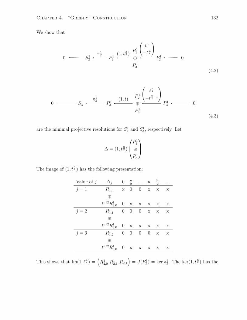
Chapter 4. “Greedy” Construction 132
We show that
0 S12 P 1
2
P 11
⊕P 13
P 12 0
π12 (1, t
n2 )
(tn
−tn2
)
(4.2)
0 S13 P 1
3
P 12
⊕P 13
P 13 0
π13 (1, t)
(tn2
−tn2−1
)
(4.3)
are the minimal projective resolutions for S12 and S1
3 , respectively. Let
∆ = (1, tn2 )
P11
⊕P 13
The image of (1, t
n2 ) has the following presentation:
Value of j ∆j 0 n2
. . . n 3n2
. . .
j = 1 R11,0 x 0 0 x x x
⊕tn/2R1
3,0 0 x x x x x
j = 2 R11,1 0 0 0 x x x
⊕tn/2R1
3,0 0 x x x x x
j = 3 R11,2 0 0 0 0 x x
⊕tn/2R1
3,0 0 x x x x x
This shows that Im(1, tn2 ) =
(R1
2,0 R12,1 R2,1
)= J(P 1
2 ) = kerπ12. The ker(1, t
n2 ) has the
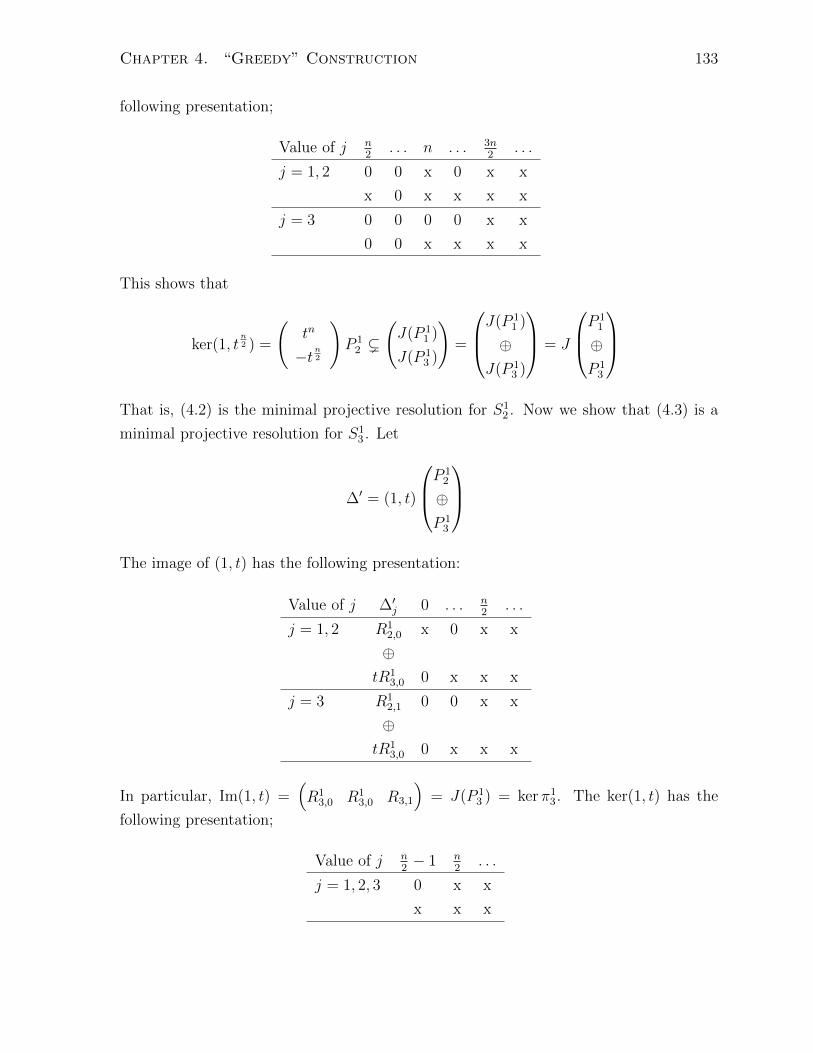
Chapter 4. “Greedy” Construction 133
following presentation;
Value of j n2
. . . n . . . 3n2
. . .
j = 1, 2 0 0 x 0 x x
x 0 x x x x
j = 3 0 0 0 0 x x
0 0 x x x x
This shows that
ker(1, tn2 ) =
(tn
−tn2
)P 12 (
(J(P 1
1 )
J(P 13 )
)=
J(P 11 )
⊕J(P 1
3 )
= J
P11
⊕P 13
That is, (4.2) is the minimal projective resolution for S1
2 . Now we show that (4.3) is a
minimal projective resolution for S13 . Let
∆′ = (1, t)
P12
⊕P 13
The image of (1, t) has the following presentation:
Value of j ∆′j 0 . . . n2
. . .
j = 1, 2 R12,0 x 0 x x
⊕tR1
3,0 0 x x x
j = 3 R12,1 0 0 x x
⊕tR1
3,0 0 x x x
In particular, Im(1, t) =(R1
3,0 R13,0 R3,1
)= J(P 1
3 ) = kerπ13. The ker(1, t) has the
following presentation;
Value of j n2− 1 n
2. . .
j = 1, 2, 3 0 x x
x x x
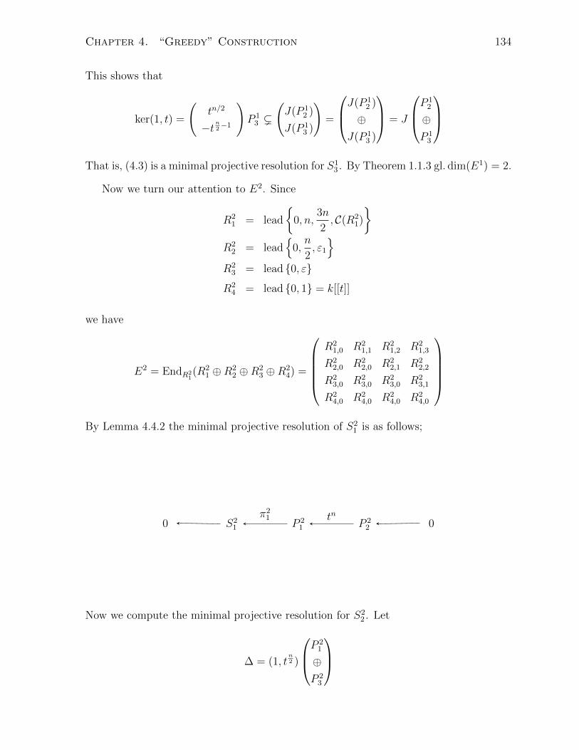
Chapter 4. “Greedy” Construction 134
This shows that
ker(1, t) =
(tn/2
−tn2−1
)P 13 (
(J(P 1
2 )
J(P 13 )
)=
J(P 12 )
⊕J(P 1
3 )
= J
P12
⊕P 13
That is, (4.3) is a minimal projective resolution for S1
3 . By Theorem 1.1.3 gl. dim(E1) = 2.
Now we turn our attention to E2. Since
R21 = lead
{0, n,
3n
2, C(R2
1)
}R2
2 = lead{
0,n
2, ε1
}R2
3 = lead {0, ε}
R24 = lead {0, 1} = k[[t]]
we have
E2 = EndR21(R2
1 ⊕R22 ⊕R2
3 ⊕R24) =
R2
1,0 R21,1 R2
1,2 R21,3
R22,0 R2
2,0 R22,1 R2
2,2
R23,0 R2
3,0 R23,0 R2
3,1
R24,0 R2
4,0 R24,0 R2
4,0
By Lemma 4.4.2 the minimal projective resolution of S2
1 is as follows;
0 S21 P 2
1 P 22 0
π21 tn
Now we compute the minimal projective resolution for S22 . Let
∆ = (1, tn2 )
P21
⊕P 23

Chapter 4. “Greedy” Construction 135
The image of (1, tn2 ) has the following presentation:
Value of j ∆j 0 n2
ε1 . . . n . . . 3n2
. . . C(R21) . . .
j = 1 R21,0 x 0 0 0 x 0 x 0 x x
⊕tn/2R2
3,0 0 x x x x x x x x x
j = 2 R21,1 0 0 0 0 x 0 x 0 x x
⊕tn/2R2
3,0 0 x x x x x x x x x
j = 3 R21,2 0 0 0 0 0 0 x 0 x x
⊕tn/2R2
3,0 0 x x x x x x x x x
j = 4 R21,3 0 0 0 0 0 0 0 0 x x
⊕tn/2R2
3,1 0 0 x x x x x x x x
That is, Im(1, tn2 ) = J(P 2
2 ) = ker π22. The ker(1, t
n2 ) has the following presentation:
Value of j n2
n ε2 . . . 3n2
. . . C(R21) . . .
j = 1, 2 0 x 0 0 x 0 x x
x x x x x x x x
j = 3 0 0 0 0 x 0 x x
0 x x x x x x x
j = 4 0 0 0 0 0 0 x x
0 0 x x x x x x
This shows that ker(1, tn2 ) =
(tn
−tn2
)P 22 . Hence,
0 S22 P 2
2
P 21
⊕P 23
P 22 0
π22 (1, t
n2 )
(tn
−tn2
)

Chapter 4. “Greedy” Construction 136
is a projective resolution for S22 and it is minimal by Proposition 2.3.6. Let
∆′ = (1, tε)
P22
⊕P 24
Then
Value of j ∆′j 0 ε . . . n2
. . . ε1 . . .
j = 1, 2 R22,0 x 0 0 x 0 x x
⊕tεR2
4,0 0 x x x x x x
j = 3 R22,1 0 0 0 x 0 x x
⊕tεR2
4,0 0 x x x x x x
j = 4 R22,2 0 0 0 0 0 x x
⊕tεR2
4,0 0 x x x x x x
That is, Im(1, tε) = J(P 23 ) = ker π2
3. The ker(1, tε) has the following presentations:
Value of j n2− ε n
2. . . ε1 . . .
j = 1, 2, 3 0 x 0 x x
x x x x x
j = 4 0 0 0 x x
0 x x x x
That is,
ker(1, tε) =
(tn2
−tn2−ε
)P 23
Hence,
0 S23 P 2
3
P 22
⊕P 24
P 23 0
π23 (1, tε)
(tn2
−tn2−ε
)
is a projective resolutions for S23 . Proposition 2.4.3 gives pdE2(S2
4) = 2, and the result

Chapter 4. “Greedy” Construction 137
follows by Theorem 1.1.3.
Notation 4.4.4. For i ≥ 3, let
εi = C(Ri1)−
3n
2, εi1 = C(Ri
1)− n, εi2 = C(Ri1)−
n
2
Lemma 4.4.5. Suppose {Ri1 : i ∈ N} is a family of starting rings constructed in section
2.5.
(a) If i ≥ 2, then the minimal projective resolutions of Sili−1 and Sili are as follows;
0 Sili−1 P ili−1
P ili−2
⊕P ili
P ili−1 0
πili−1 (1, tε)
(tn2
−tn2−ε
)
(4.4)
0 Sili P ili
P ili−1
⊕P ili
P ili
0πili (1, t)
(tε
−tε−1
)
(4.5)
(b) For all i ∈ N we have
0 Si2 P i2
P i1
⊕P i3
P i2 0
πi2 (1, tn2 )
(tn
−tn2
)
(4.6)
(c) For i ≥ 3, the minimal projective resolution of Si3 is as follows;
0 Si3 P i3
P i2
⊕P i4
P i3 0
πi3 (1, tn2 )
(tn2
−1
)
(4.7)
Warning that parts (a) and (c) are false for i = 1 (see Lemma 4.4.3).

Chapter 4. “Greedy” Construction 138
Proof. (a) Fix i ≥ 2. Lemma 4.4.1(d) yields
Rili−2 = lead
{0,n
2, ε1
}Rili−1 = lead {0, ε}
Rili
= k[[t]]
In particular,
(P ili−2)j =
Rili−2,0 if 1 ≤ j ≤ li − 2
Rili−2,1 if j = li − 1
Rli−2,2 if j = li
(P ili−1)j =
Rili−1,0 if 1 ≤ j ≤ li − 1
Rili−1,1 if j = li
=⇒ J(P ili−1)j =
Rili−1,0 if 1 ≤ j ≤ li − 2
Rili−1,1 if j = li − 1, li
,
(P ili)j = Ri
li,0for 1 ≤ j ≤ li =⇒ (J(P i
li))j =
Rili,0
if 1 ≤ j ≤ li − 1
Rli,1 if j = li
Let
∆ = (1, tε)
Pili−2
⊕P ili
Then
Value of j ∆j 0 1 . . . ε . . . n2
. . . ε1 . . .
1 ≤ j ≤ li − 2 Rili−2,0 x 0 0 0 0 x 0 x x
⊕tεRi
li,00 0 0 x x x x x x
j = li − 1 Rili−2,1 0 0 0 0 0 x 0 x x
⊕tεRi
li,00 0 0 x x x x x x
j = li Rili−2,2 0 0 0 0 0 0 0 x x
⊕tεRi
li,00 0 0 x x x x x x
That is, Im(1, tε) = J(P ili−1) = kerπili−1. Moreover, ker(1, tε) has the following presenta-
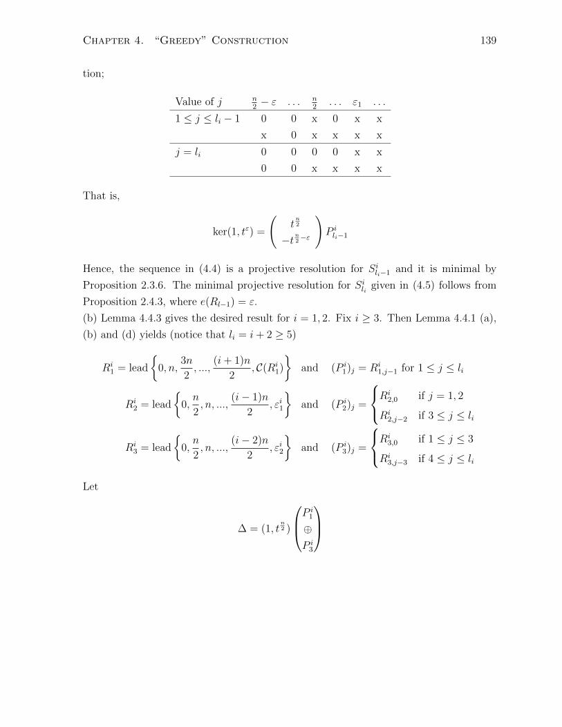
Chapter 4. “Greedy” Construction 139
tion;
Value of j n2− ε . . . n
2. . . ε1 . . .
1 ≤ j ≤ li − 1 0 0 x 0 x x
x 0 x x x x
j = li 0 0 0 0 x x
0 0 x x x x
That is,
ker(1, tε) =
(tn2
−tn2−ε
)P ili−1
Hence, the sequence in (4.4) is a projective resolution for Sili−1 and it is minimal by
Proposition 2.3.6. The minimal projective resolution for Sili given in (4.5) follows from
Proposition 2.4.3, where e(Rl−1) = ε.
(b) Lemma 4.4.3 gives the desired result for i = 1, 2. Fix i ≥ 3. Then Lemma 4.4.1 (a),
(b) and (d) yields (notice that li = i+ 2 ≥ 5)
Ri1 = lead
{0, n,
3n
2, ...,
(i+ 1)n
2, C(Ri
1)
}and (P i
1)j = Ri1,j−1 for 1 ≤ j ≤ li
Ri2 = lead
{0,n
2, n, ...,
(i− 1)n
2, εi1
}and (P i
2)j =
Ri2,0 if j = 1, 2
Ri2,j−2 if 3 ≤ j ≤ li
Ri3 = lead
{0,n
2, n, ...,
(i− 2)n
2, εi2
}and (P i
3)j =
Ri3,0 if 1 ≤ j ≤ 3
Ri3,j−3 if 4 ≤ j ≤ li
Let
∆ = (1, tn2 )
Pi1
⊕P i3
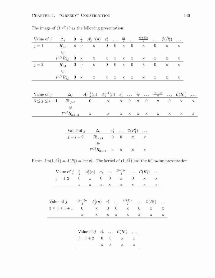
Chapter 4. “Greedy” Construction 140
The image of (1, tn2 ) has the following presentation:
Value of j ∆j 0 n2
Ai−12 (n) εi1 . . . in2
. . . (i+1)n2
. . . C(Ri1) . . .
j = 1 Ri1,0 x 0 x 0 0 x 0 x 0 x x
⊕tn/2Ri
3,0 0 x x x x x x x x x x
j = 2 Ri1,1 0 0 x 0 0 x 0 x 0 x x
⊕tn/2Ri
3,0 0 x x x x x x x x x x
Value of j ∆j Aj−1j−2(n) Ai−1j (n) εi1 . . . in2
. . . (i+1)n2
. . . C(Ri1) . . .
3 ≤ j ≤ i+ 1 Ri1,j−1 0 x x 0 x 0 x 0 x x
⊕tn/2Ri
3,j−3 x x x x x x x x x x
Value of j ∆j εi1 . . . C(Ri1) . . .
j = i+ 2 Ri1,i+1 0 0 x x
⊕tn/2Ri
3,i−1 x x x x
Hence, Im(1, tn2 ) = J(P i
2) = ker πi2. The kernel of (1, tn2 ) has the following presentation:
Value of j n2
Ai2(n) εi2 . . . (i+1)n2
. . . C(Ri1) . . .
j = 1, 2 0 x 0 0 x 0 x x
x x x x x x x x
Value of j (j−1)n2
Aij(n) εi2 . . . (i+1)n2
. . . C(Ri1) . . .
3 ≤ j ≤ i+ 1 0 x 0 0 x 0 x x
x x x x x x x x
Value of j εi2 . . . C(Ri1) . . .
j = i+ 2 0 0 x x
x x x x

Chapter 4. “Greedy” Construction 141
Therefore,
ker(1, tn2 ) =
(tn
−tn2
)P i2
That is, (4.6) is a projective resolution for Si2, and they are minimal by Proposition 2.3.6.
(c) Fix i ≥ 3, then li = i+ 2 ≥ 5. Lemma 4.4.1 (a), (b) and (d) yield
Ri1 = lead
{0, n,
3n
2, ...,
(i+ 1)n
2, tC(R
i1)
}and (P i
1)j = Ri1,j−1 for 1 ≤ j ≤ li
Ri2 = lead
{0,n
2, n, ...,
(i− 1)n
2, εi1
}and (P i
2)j =
Ri2,0 if j = 1, 2
Ri2,j−2 if 3 ≤ j ≤ li
Ri3 = lead
{0,n
2, n, ...,
(i− 2)n
2, εi}
and (P i3)j =
Ri3,0 if 1 ≤ j ≤ 3
Ri3,j−3 if 4 ≤ j ≤ li
Ri4 = lead
{0,n
2, n, ...,
(i− 3)n
2, C(Ri
1)− 2n
}and (P i
4)j =
Ri4,0 if 1 ≤ j ≤ 4
Ri4,j−4 if 5 ≤ j ≤ li
Let a ≤ b be natural numbers and define
∆ = (1, tn2 )
Pi2
⊕P i4
Then
Value of j ∆j 0 Ai−21 (n) εi . . . (i−1)n2
. . . εi1 . . .
j = 1, 2 Ri2,0 x x 0 0 x 0 x x
⊕tn/2Ri
4,0 0 x x x x x x x
j = 3 Ri2,1 0 x 0 0 x 0 x x
⊕tn/2Ri
4,0 0 x x x x x x x

Chapter 4. “Greedy” Construction 142
Value of j ∆j(j−3)n
2Ai−2j−2(n) εi . . . (i−1)n
2. . . εi1 . . .
4 ≤ j ≤ i+ 1 Ri2,j−2 0 x 0 0 x 0 x x
⊕tn/2Ri
4,j−4 x x x x x x x x
Value of j ∆j εi . . . εi1 . . .
j = i+ 2 Ri1,i+1 0 0 x x
⊕tn/2Ri
3,i−1 x x x x
Hence, Im(1, tn2 ) = J(P i
3) = ker πi3. The kernel of (1, tn2 ) has the following presentation:
Value of j 0 Ai−21 (n) εi . . . (i−1)n2
. . . εi1 . . .
1 ≤ j ≤ 3 0 x 0 0 x 0 x x
x x x x x x x x
Value of j (j−3)n2
Ai−2j−2(n) εi . . . (i−1)n2
. . . εi1 . . .
4 ≤ j ≤ i+ 1 0 x 0 0 x 0 x x
x x x x x x x x
Value of j εi . . . εi1 . . .
j = i+ 2 0 0 x x
x x x x
Therefore,
ker(1, tn2 ) =
(tn2
−1
)P i3
That is, (4.7) is a projective resolution for Si3, and it is minimal by Proposition 2.3.6.
Lemma 4.4.6. The minimal projective resolutions of the simple E3-modules are as fol-
lows;
0 S31 P 3
1 P 32 0
π31 tn

Chapter 4. “Greedy” Construction 143
0 S32 P 3
2
P 31
⊕P 33
P 32 0
π32 (1, t
n2 )
(tn
−tn2
)
0 S33 P 3
3
P 32
⊕P 34
P 33 0
π33 (1, t
n2 )
(tn2
−1
)
0 S34 P 3
4
P 33
⊕P 35
P 34 0
π34 (1, tε)
(tn2
−tn2−ε
)
0 S35 P 3
5
P 34
⊕P 35
P 35 0
π35 (1, t)
(tε
−tε−1
)
Proof. By Lemma 4.4.1(a) l3 = 5. The minimal projective resolutions follow from Lem-
mas 4.4.2 and 4.4.5.
We now prove the third main result of this thesis.
Theorem 4.4.7. Let {Ri1| i ∈ N} be a set of starting rings constructed in section 2.5.

Chapter 4. “Greedy” Construction 144
(a) For i ≥ 3, the minimal projective resolutions of the simple Ei-modules are as follows:
0 Si1 P i1 P i
2 0πi1 tn
(4.8)
0 Si2 P i2
P i1
⊕P i3
P i2 0
πi2 (1, tn2 )
(tn
−tn2
)
(4.9)
0 Sili−1 P ili−1
P ili−2
⊕P ili
P ili−1 0
πili−1 (1, tε)
(tn2
−tn2−ε
)
(4.10)
0 Sili P ili
P ili−1
⊕P ili
P ili
0πili (1, t)
(tε
−tε−1
)
(4.11)
and for 3 ≤ j ≤ li − 2,
0 Sij P ij
P ij−1
⊕P ij+1
P ij 0
πij (1, tn2 )
(tn2
−1
)
(4.12)
(b) gl. dim(Ei) = 2 for all i ∈ N.
Proof. (a) We proceed by induction on i. The result is true for E3 by Lemma 4.4.6.
Assume the result is true for i − 1 ≥ 3. Lemmas 4.4.2 and 4.4.5 gives us the exact
sequences (4.8), (4.9), (4.10), (4.11), and the minimal projective resolution of Si3. If
4 ≤ j ≤ li − 2, the minimal projective resolution of Sij has the following beginning by
Theorem 1.1.4;
0 Sij P ij
πij

Chapter 4. “Greedy” Construction 145
More specifically, we have the following short exact sequence;
0 Sij P ij J(P i
j ) 0πij inc
(4.13)
where inc is the inclusion map. Since i, j ≥ 4, Proposition 4.4.1(e) yields (J(P i−1j−1))d1e =
J(P ij ). By the induction hypothesis, the following sequence is exact:
0 Si−1j−1 P i−1j−1
P i−1j−2
⊕P i−1j
P i−1j−1 0
πi−1j−1 (1, tn2 )
(tn2
−1
)
Since Im(1, tn2 ) = ker(πi−1j−1) = J(P i−1
j−1), we get the following short exact sequence;
0 J(P i−1j−1)
P i−1j−2
⊕P i−1j
P i−1j−1 0
(1, tn2 )
(tn2
−1
)
By Lemma 2.6.5, the following sequence is exact:
0 J(P i−1j−1)d1e
P i−1j−2d1e⊕
P i−1j d1e
P i−1j−1d1e 0
(1, tn2 )
(tn2
−1
)
By Lemma 4.4.1(e) the above short exact sequence is the short exact sequence
0 J(P ij )
P ij−1
⊕P ij+1
P ij 0
(1, tn2 )
(tn2
−1
)
(4.14)
Splicing sequences (4.13) and (4.14) gives the following projective resolution for Sij;

Chapter 4. “Greedy” Construction 146
0 Sij P ij
P ij−1
⊕P ij+1
P ij 0
πij (1, tn2 )
(tn2
−1
)
By Proposition 2.3.6, the projective resolutions are minimal.
(b) This is a direct consequence of part (a), Theorem 1.1.3 and Lemma 4.4.3.

Chapter 5
Examples and Open Questions
In this chapter we give an example illustrating the possible values for global dimension
of E when the only restriction on its construction is the one given in section 2.2. We
conclude with some open questions which could be used for future research.
We start by recalling the restriction in section 2.2. Suppose H is a numerical semi-
group with generators α1, α2, ..., αs, F (α1, α2, ..., αs) > −1, and let R1 be the ring of for-
mal power series associated to H. Since R1 6= R̃1 = k[[t]], we have R1 ( EndR1(m1) ⊆ R̃1
(Theorem 1.1.1). Moreover, m1 contains a non-zero divisor (Proposition 2.2.1), and
EndR1(m1) embeds naturally into R1 (by sending f to f(a)/a, which is independent of
the non-zero divisor a ∈ m1). It is well known that in fact EndR1(m1) ⊆ R̃1. Further-
more, it is easy to see that EndR1(m1) is itself a ring of formal power series. Let R2
be any ring of formal power series over k that properly contains R1 and is contained
in EndR1(m1). Notice that R2 is a local Noetherian ring of (Krull) dimension 1. If
R2 = k[[t]], then R2 = EndR1(m1) = k[[t]] in which case we define
M := R1 ⊕R2, E := EndR1(M)
If R2 6= k[[t]], pick R3 such that R2 ( R3 ⊆ EndR1(m2) ⊆ k[[t]] (this is possible by
Theorem 1.1.1). If R3 = k[[t]], define
M := R1 ⊕R2 ⊕R3, E := EndR1(M)
Notice that R1 ( R2 ( R3 = k[[t]]. If R3 6= k[[t]], repeat the process to obtain R4, and
continue in this fashion. Since R1 is missing only finitely many powers of t there exists
an l such that Rl = R̃1 = k[[t]]. Hence, we have constructed an ascending chain of rings
R1 ( R2 ( R3 ( ... ( Rl−1 ( Rl = k[[t]]
147
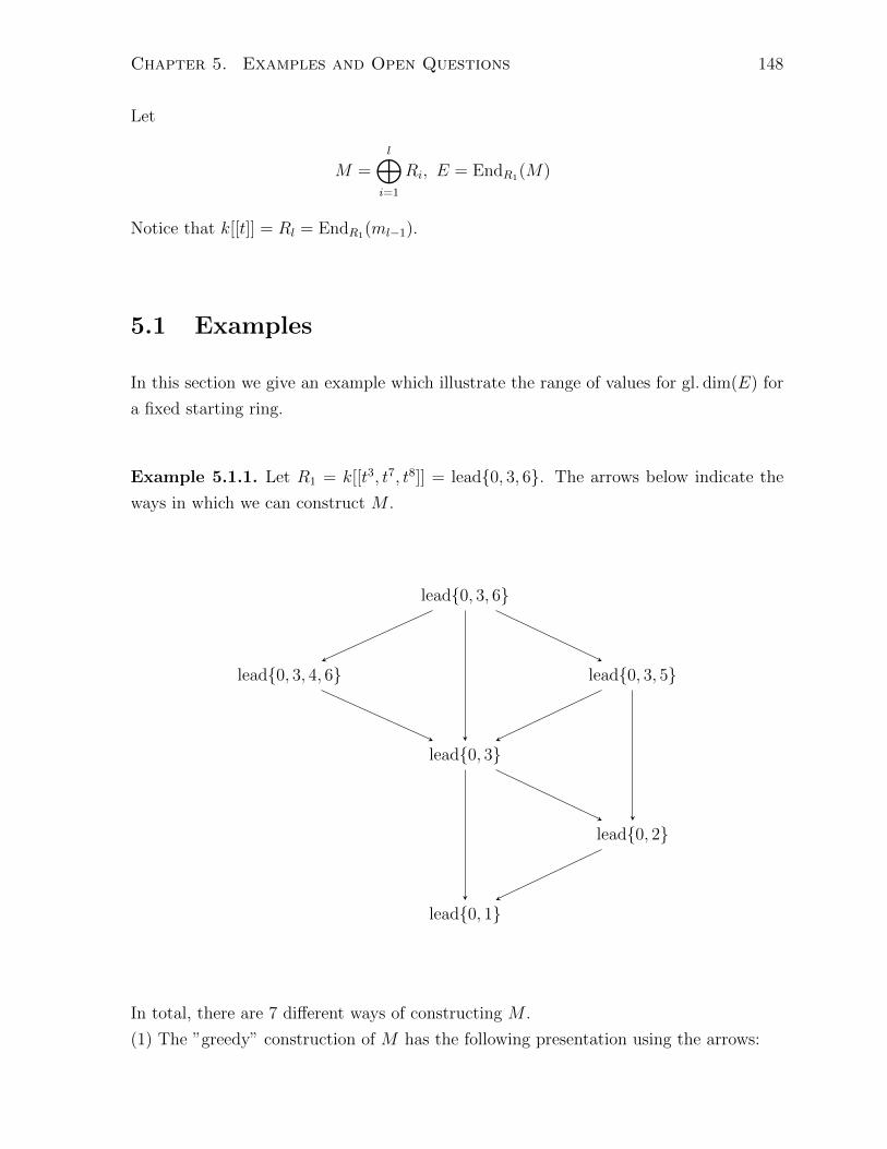
Chapter 5. Examples and Open Questions 148
Let
M =l⊕
i=1
Ri, E = EndR1(M)
Notice that k[[t]] = Rl = EndR1(ml−1).
5.1 Examples
In this section we give an example which illustrate the range of values for gl. dim(E) for
a fixed starting ring.
Example 5.1.1. Let R1 = k[[t3, t7, t8]] = lead{0, 3, 6}. The arrows below indicate the
ways in which we can construct M .
lead{0, 3, 6}
lead{0, 3, 4, 6} lead{0, 3, 5}
lead{0, 3}
lead{0, 2}
lead{0, 1}
In total, there are 7 different ways of constructing M .
(1) The ”greedy” construction of M has the following presentation using the arrows:

Chapter 5. Examples and Open Questions 149
R1 = lead{0, 3, 6}
R2 = lead{0, 3}
R3 = lead{0, 1}
Then, gl. dim(E) = 2 by Lemma 4.2.2.
(2) The ”lazy” construction of M has the following presentation using the arrows:
R1 = lead{0, 3, 6}
R2 = lead{0, 3, 5}
R3 = lead{0, 3}
R4 = lead{0, 2}
R5 = lead{0, 1}
Then, gl. dim(E) = 2 by Lemma 3.2.3.
(3) The third construction of M has the following presentation using the arrows;

Chapter 5. Examples and Open Questions 150
R1 = lead{0, 3, 6}
R2 = lead{0, 3}
R3 = lead{0, 2}
R4 = lead{0, 1}
Then
E =
R1 t3R2 t6R4 t6R4
R2 R2 t3R4 t3R4
R3 R3 R3 t2R4
R4 R4 R4 R4
The minimal projective resolutions for the simple modules are as follows;
0 S1 P1 P2 0π1 t3
0 S2 P2
P1
⊕P4
P2 0π2 (1, t3)
(t3
−1
)
0 S3 P3
P2
⊕P4
P4 0π3 (1, t2)
(t3
−t2
)
0 S4 P4
P3
⊕P4
P4 0π4 (1, t)
(t2
−t
)
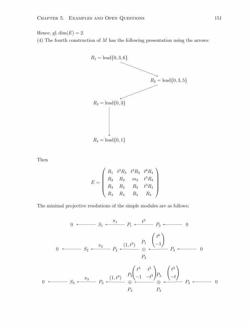
Chapter 5. Examples and Open Questions 151
Hence, gl. dim(E) = 2.
(4) The fourth construction of M has the following presentation using the arrows:
R1 = lead{0, 3, 6}
R2 = lead{0, 3, 5}
R3 = lead{0, 3}
R4 = lead{0, 1}
Then
E =
R1 t3R3 t3R3 t6R4
R2 R2 m2 t5R4
R3 R3 R3 t3R4
R4 R4 R4 R4
The minimal projective resolutions of the simple modules are as follows;
0 S1 P1 P3 0π1 t3
0 S2 P2
P1
⊕P4
P4 0π2 (1, t5)
(t6
−1
)
0 S3 P3
P2
⊕P4
P3
⊕P4
P4 0π3 (1, t3)
(t3 t5
−1 −t2
) (t3
−t
)

Chapter 5. Examples and Open Questions 152
0 S4 P4
P3
⊕P4
P4 0π4 (1, t)
(t3
−t2
)
Hence, gl. dim(E) = 3.
(5) The fifth construction of M has the following presentation using the arrows:
R1 = lead{0, 3, 6}
R2 = lead{0, 3, 4, 6}
R3 = lead{0, 3}
R4 = lead{0, 2}
R5 = lead{0, 1}
Then
E =
R1 t3R3 t3R3 t6R5 t6R5
R2 R2 m2 t4R4 t6R5
R3 R3 R3 t3R5 t3R5
R4 R4 R4 R4 t2R5
R5 R5 R5 R5 R5
The minimal projective resolutions of the simple modules are as follows;
0 S1 P1 P3 0π1 t3
0 S2 P2
P1
⊕P4
P5 0π2 (1, t4)
(t6
−t2
)

Chapter 5. Examples and Open Questions 153
0 S3 P3
P2
⊕P5
P3
⊕P4
P5 0π3 (1, t3)
(t3 t4
−1 −t
) (t3
−t2
)
0 S4 P4
P3
⊕P5
P5 0π4 (1, t2)
(t3
−t
)
0 S5 P5
P4
⊕P5
P5 0π5 (1, t)
(t2
−t
)
Hence, gl. dim(E) = 3.
(6) The sixth construction of M has the following presentation using the arrows:
R1 = lead{0, 3, 6}
R2 = lead{0, 3, 4, 6}
R3 = lead{0, 3}
R4 = lead{0, 1}
Then
E =
R1 t3R3 t3R3 t6R4
R2 R2 m2 t6R4
R3 R3 R3 t3R4
R4 R4 R4 R4
The minimal projective resolutions of the simple modules are as follows;

Chapter 5. Examples and Open Questions 154
0 S1 P1 P3 0π1 t3
0 S2 P2
P1
⊕P3
P4 0π2 (1, t4)
(t7
−t3
)
0 S3 P3
P2
⊕P4
P3
⊕P3
P4 0π3 (1, t3)
(t3 t4
−1 −t
) (t4
−t3
)
0 S4 P4
P3
⊕P4
P4 0π4 (1, t)
(t3
−t2
)
Hence, gl. dim(E) = 3.
(7) The seventh construction of M has the following presentation using the arrows:
R1 = lead{0, 3, 6}
R2 = lead{0, 3, 5}
R3 = lead{0, 2}
R4 = lead{0, 1}
Then
E =
R1 m1 t6R4 t6R4
R2 R2 t3R3 t5R4
R3 R3 R3 t2R4
R4 R4 R4 R4
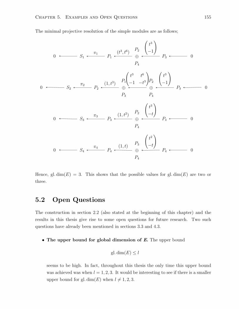
Chapter 5. Examples and Open Questions 155
The minimal projective resolution of the simple modules are as follows;
0 S1 P1
P2
⊕P4
P3 0π1 (t3, t6)
(t3
−1
)
0 S2 P2
P1
⊕P3
P2
⊕P4
P3 0π2 (1, t3)
(t3 t6
−1 −t3
) (t3
−1
)
0 S3 P3
P2
⊕P4
P4 0π3 (1, t2)
(t3
−t
)
0 S4 P4
P3
⊕P4
P4 0π4 (1, t)
(t2
−t
)
Hence, gl. dim(E) = 3. This shows that the possible values for gl. dim(E) are two or
three.
5.2 Open Questions
The construction in section 2.2 (also stated at the beginning of this chapter) and the
results in this thesis give rise to some open questions for future research. Two such
questions have already been mentioned in sections 3.3 and 4.3.
• The upper bound for global dimension of E. The upper bound
gl. dim(E) ≤ l
seems to be high. In fact, throughout this thesis the only time this upper bound
was achieved was when l = 1, 2, 3. It would be interesting to see if there is a smaller
upper bound for gl. dim(E) when l 6= 1, 2, 3.

Chapter 5. Examples and Open Questions 156
• Possible values for gl. dim(E). Suppose we fix a starting ring R associated to
a numerical semigroup H. The question which arises is what are the possible
values for gl. dim(E) when R is the starting ring and the only restriction on the
construction of our ascending chain is the one given in section 2.2? For example, in
section 5.1 we showed that if R = k[[t3, t7, t8]] then the possible values for gl. dim(E)
are 2 or 3.
• Other families of starting rings. The family of starting rings constructed in
section 2.5 leads to the question of whether it is possible to construct other families
of starting rings with analogous results given in this thesis. Also, it would be inter-
esting to construct other families of starting rings with new results for gl. dim(E).
• Projective dimension of the first and second simple module. The results
in this thesis suggest that
pdE(S1) ≤ pdE(S2).
Furthermore, under the lazy construction they suggest that
pdE(S1) ≤ pdE(S2) ≤ pdE(S1) + 1.
• Values of l. Fix a starting ring R. Let Rchain be the set of all ascending chains
such that R is the starting ring in the chain, and the chain satisfies the condition
given in section 2.2. Moreover, let Rlength be the set consisting of the lengths of the
chains that appear in Rchain. Since R is associated to some semigroup, Rchain is a
finite set, hence, Rlength is a finite set. We know that Rlength is bounded above by
g(R) + 1. It would be interesting to know all the elements of Rlength or to obtain a
lower bound for Rlength. For example, if R = k[[t3, t7, t8]], then example 5.1.1 shows
that Rlength = {3, 4, 5}.

Bibliography
[1] Michael Atiyah, On the Krull-Schmidt theorem with application to sheaves. Bull.
Soc. Math. France 84 (1956), 307 - 317. MR0086358 (19,172b)
[2] Maurice Auslander, Idun Reiten, and O. Sverre Smal∅. Representation theory of
Artin algebras. Corrected reprint of the 1995 original. Cambridge Studies in Ad-
vanced Mathematics, 36. Cambridge University Press, Cambridge, 1997. MR1476671
(98e:16011)
[3] Hyman Bass, Algebraic K-theory. W. A. Benjamin, Inc., New York-Amsterdam,
1968. MR0249491
[4] H. Grauert and R. Remmert, Analytische Stellenalgebren. (German) Unter Mitar-
beit von ). Riemenschneider. Die Grundlehren der mathematischen Wissenschaften,
Band 176. Springer-Verlag, Berlin-New York, 1971. MR0316742 (47:5290)
[5] Jooyoun Hong, Bernd Ulrich, and V. Wolmer Vasconcelos, Normalization of
modules. J. Algebra 303 (2006), no. 1, 133-145. MR2253656 (20073:13006)
[6] Osamu Iyama, τ -categories. II. Nakayama pairs and rejective subcategories. Al-
gebr. Represent. Theory 8 (2005), no. 4, 449-477. MR2199205 (2006i:18013)
[7] Osamu Iyama, Rejective subcategories of artin algebras and orders. arXiv
0311281v1, 2003.
[8] Nathan Jacobson, Basic Algebra I. Second edition. W. H. Freeman and Company,
New York, 1985. MR0780184 (86d:00001)
[9] Nathan Jacobson. Basic Algebra II. Second edition. W. H. Freeman and Company,
New York, 1989. MR1009787 (90d:00007)
[10] Henning Krause, Krull-Schmidt categories and projective covers. Expo. Math. 33
(2015), no. 4, 535-549. MR3431480
157

Bibliography 158
[11] Graham J. Leuschke, Endomorphism rings of finite global dimension. Canad.
J. Math, 59, no.2, (2007), 332-343. MR2310620 (2008c:16019)
[12] Hideyuki Matsumura, Commutative Ring Theory. Translated from the Japanese
by M. Reid. Second edition. Cambridge Studies in Advanced Mathematics, vol. 8.
Cambridge University Press, Cambridge, 1989. MR1011461 (90i:13001)
[13] J. C. McConnell and J. C. Robson, Noncommutative Noetherian rings. With the
cooperation of L. W. Small. Revised edition. Graduate studies in Mathematics, 30.
American Mathematical Society, Providence, RI, 2001. MR1811901 (2001i:16039)
[14] Amnon Neeman, Triangulated Categories. Annals of Mathematics Studies, 148.
Princeton University Press, Princeton, NJ, 2001. MR1812507 (2001k:18010)
[15] Irving Reiner, Maximal orders. Corrected reprint of the 1975 original. With a
foreword by M. J. Taylor. London Mathematical Society Monographs, New Se-
ries, 28. The Clarendon Press, Oxford University Press, Oxford, 2003. MR1972204
(2004c:16026)
[16] Irving Reiner, Maximal orders. London Mathematical Society Monographs, no. 5.
Academic Press [A subsidiary of Harcourt Brace Jovanovich, Publishers], London-
New York, 1975. MR0393100 (52:13910)
[17] J.Joseph Rotman, An introduction to homological algebra, second edition. Univer-
sitext. Springer, New York, 2009. MR2455920 (2009i:18011)
[18] J. C. Rosales and P. A. Garcia-Sanchez, Numerical semigroups, Developments in
Mathematics, 20. Springer, New York, 2009. MR2549780 (2010j:20091)
[19] J. C. Rosales and P. A. Garcia-Sanchez, Finitely generated commutative monoids,
Nova Science Publishers, Inc., Commack, New York, 1999. MR1694173
(2000d:20074)
[20] J. J. Sylvester. “Mathematical questions with their solutions”. Educational times,
41 (21), 1884.
[21] V. Wolmer Vasconcelos, On the radical of endomorphism rings of local modules.
Bull. Braz. Math. Soc. (N.S.) 45 (2014), no.4, 871-886. MR3296198