constraints and invariance in target detection
TRANSCRIPT

Constraints and invariance in target detection
By Frederick Nicolls
Thesis presented for the Degree of Doctor of Philosophy,Department of Electrical Engineering,University of Cape Town.Cape Town, February 2000


Constraints and invariance in target detection
Frederick NicollsFebruary 2000
Abstract
The concept of invariance in hypothesis testing is discussed for purposes of target detection. Invarianttests are proposed and analysed in two contexts.
The first involves the use of cyclic permutation invariance as a solution to detecting targets with un-known location in noise. An invariance condition is used to eliminate the target location parameter, anda uniformly most powerful test developed for the reduced data. The test is compared with conventionalsolutions, and shown to be more powerful. The difference however is slight, justifying the simplerformulations. This conclusion continues to hold even when additional unknown noise parameters areintroduced.
The second form of invariance involves invariance to data contained in linear subspaces of the obser-vation space. Such invariance is proposed as a generic method of reducing mismatch resulting fromoverly-simple models, which cannot capture the full complexity of the data. The formulation involvesa data-reducing projection, where components of the data which are difficult to model are discarded.The notion has relevance to both low-rank subspace interference and low-rank subspace mismatch.
Methods are presented for making estimates of invariance subspaces and covariance matrices for usein this invariant detection formulation. Using two different interpretations, necessary conditions on thesubspace estimates are derived. These conditions can sometimes be solved exactly, but approximatemethods are provided for the general case. It is shown that for use in invariant detectors, covariancematrix estimates have to be independent of data components contained in the invariance subspace. TheEM algorithm can be appropriate for this estimation. Maximum likelihood methods for obtaining theestimates are presented under Toeplitz, circulant, doubly block Toeplitz, and ARMA constraints.
Using actual samples of x-ray data, results are presented which demonstrate that subspace invariant testscan be substantially more predictable than noninvariant tests. This is true in particular when modelsare highly constrained, as is commonly necessary in adaptive detection. The improved predictabilityusually comes at the cost of a decrease in performance, although this is not always so. The invariantdetectors also avoid the need to preprocess data to better fit the assumptions.
i

ii

Acknowledgements
• The financial assistance of the National Research Foundation towards this research is herebyacknowledged. Opinions expressed in this work, or conclusions arrived at, are those of theauthor and are not necessarily to be attributed to the National Research Foundation.
• The financial assistance of De Beers Consolidated Mines Limited is also acknowledged.
iii

iv
Contents
Abstract i
Acknowledgements iii
Table of Contents v
Acronyms xi
1 Introduction 1
1.1 Description of the general problem . . . . . . . . . . . . . . . . . . . . . . . . . . . 1
1.2 Overview of statistical hypothesis testing . . . . . . . . . . . . . . . . . . . . . . . 3
1.3 The GLRT as a testing philosophy . . . . . . . . . . . . . . . . . . . . . . . . . . . 7
1.4 Specifying the conditional density of the noise . . . . . . . . . . . . . . . . . . . . . 10
1.5 Constraints and invariance in testing . . . . . . . . . . . . . . . . . . . . . . . . . . 12
1.5.1 Constraints in hypothesis testing . . . . . . . . . . . . . . . . . . . . . . . . 12
1.5.2 Invariance in hypothesis testing . . . . . . . . . . . . . . . . . . . . . . . . 14
1.6 Subspace invariance in adaptive detection . . . . . . . . . . . . . . . . . . . . . . . 17
1.7 Thesis outline and description . . . . . . . . . . . . . . . . . . . . . . . . . . . . . 19
1.7.1 Detection of targets with unknown location . . . . . . . . . . . . . . . . . . 20
1.7.2 Subspace invariance in detection . . . . . . . . . . . . . . . . . . . . . . . . 21
1.7.3 Subspace invariant covariance estimation . . . . . . . . . . . . . . . . . . . 23
1.7.4 Adaptive detection with invariance . . . . . . . . . . . . . . . . . . . . . . . 25
1.8 Notation and conventions . . . . . . . . . . . . . . . . . . . . . . . . . . . . . . . . 26
v
CONTENTS
2 Review of relevant literature 29
2.1 General literature . . . . . . . . . . . . . . . . . . . . . . . . . . . . . . . . . . . . 30
2.2 Basic parametric detection with multiple observations . . . . . . . . . . . . . . . . . 32
2.3 Advanced parametric detection with multiple observations . . . . . . . . . . . . . . 36
2.4 Predictability of detectors . . . . . . . . . . . . . . . . . . . . . . . . . . . . . . . . 39
2.5 Invariance in detection problems . . . . . . . . . . . . . . . . . . . . . . . . . . . . 41
2.6 Other detection literature . . . . . . . . . . . . . . . . . . . . . . . . . . . . . . . . 42
2.7 Constrained covariance modelling and estimation . . . . . . . . . . . . . . . . . . . 44
3 Detection of targets with unknown location 47
3.1 GLRT formulation for circular and linear shifts . . . . . . . . . . . . . . . . . . . . 49
3.1.1 Formulation for linear shifts . . . . . . . . . . . . . . . . . . . . . . . . . . 49
3.1.2 Formulation for circular shifts . . . . . . . . . . . . . . . . . . . . . . . . . 53
3.1.3 Discussion . . . . . . . . . . . . . . . . . . . . . . . . . . . . . . . . . . . 55
3.2 UMP cyclic permutation invariant detection . . . . . . . . . . . . . . . . . . . . . . 56
3.2.1 Invariance of the hypothesis testing problem . . . . . . . . . . . . . . . . . . 57
3.2.2 Maximal invariant statistic for the problem . . . . . . . . . . . . . . . . . . 58
3.2.3 Distribution of the maximal invariant statistic . . . . . . . . . . . . . . . . . 59
3.2.4 Optimal invariant likelihood ratio test . . . . . . . . . . . . . . . . . . . . . 61
3.2.5 Prewhitening in the invariant detection problem . . . . . . . . . . . . . . . . 62
3.3 Comparison of GLRT and UMPI tests . . . . . . . . . . . . . . . . . . . . . . . . . 62
3.4 Cyclic permutation invariant detection with additional nuisance parameters . . . . . 65
3.4.1 Invariant estimation of certain circulant covariance matrices . . . . . . . . . 68
3.4.2 Invariant detection using invariant estimates of nuisance parameters . . . . . 70
3.5 Performance of GLRT with invariant estimates . . . . . . . . . . . . . . . . . . . . 71
3.6 Concluding remarks . . . . . . . . . . . . . . . . . . . . . . . . . . . . . . . . . . . 73
4 Subspace invariance in detection 77
4.1 Linear subspaces . . . . . . . . . . . . . . . . . . . . . . . . . . . . . . . . . . . . 79
vi
CONTENTS
4.2 Detection in subspace interference . . . . . . . . . . . . . . . . . . . . . . . . . . . 82
4.2.1 Detection without invariance . . . . . . . . . . . . . . . . . . . . . . . . . . 84
4.2.2 Invariant detection for subspace interference . . . . . . . . . . . . . . . . . 85
4.2.3 Discussion . . . . . . . . . . . . . . . . . . . . . . . . . . . . . . . . . . . 89
4.3 Interference subspace estimation for invariant detection . . . . . . . . . . . . . . . . 91
4.3.1 Effect of interference on sample mean and covariance . . . . . . . . . . . . 93
4.3.2 Likelihood function with interference . . . . . . . . . . . . . . . . . . . . . 96
4.3.3 Specific cases of interference subspace estimation . . . . . . . . . . . . . . . 99
4.3.4 Approximate estimate of interference subspace . . . . . . . . . . . . . . . . 103
4.3.5 Discussion . . . . . . . . . . . . . . . . . . . . . . . . . . . . . . . . . . . 105
4.3.6 Example of interference subspace estimation . . . . . . . . . . . . . . . . . 105
4.4 Subspace invariance in general testing . . . . . . . . . . . . . . . . . . . . . . . . . 109
4.5 Invariance subspace estimation for model mismatch . . . . . . . . . . . . . . . . . . 112
4.5.1 Formulation of invariance subspace estimate . . . . . . . . . . . . . . . . . 113
4.5.2 Example of invariance subspace estimation . . . . . . . . . . . . . . . . . . 116
4.6 Appendix: Some vector and matrix calculus results . . . . . . . . . . . . . . . . . . 120
4.6.1 dy/dθ of y = y(x(θ)): . . . . . . . . . . . . . . . . . . . . . . . . . . . . . 121
4.6.2 dy/dθ of y = vT (θ)w(θ): . . . . . . . . . . . . . . . . . . . . . . . . . . . 121
4.6.3 dv/dθ of v = A(θ)u(θ): . . . . . . . . . . . . . . . . . . . . . . . . . . . . 121
4.6.4 dy/dθ of y = ln |A(θ)|: . . . . . . . . . . . . . . . . . . . . . . . . . . . . 122
4.6.5 dC/dhi of C =∑m
j=1
∑mk≥ j λ j kg j k(h1, . . . , hm): . . . . . . . . . . . . . . . 123
4.6.6 dy/dUH of y = ln |UTH CUH |: . . . . . . . . . . . . . . . . . . . . . . . . . 124
4.6.7 dx j/dhi of x = UTH CUH : . . . . . . . . . . . . . . . . . . . . . . . . . . . 127
4.6.8 d f/dUH of f = xT UH(UTH CUH)−1UT
H y: . . . . . . . . . . . . . . . . . . . 127
5 Subspace invariant covariance estimation 129
5.1 Parameter estimates for subspace invariant detectors . . . . . . . . . . . . . . . . . . 133
5.1.1 Invariant estimation for plug-in detection . . . . . . . . . . . . . . . . . . . 133
5.1.2 Invariant estimation for GLRT detection . . . . . . . . . . . . . . . . . . . . 136
vii
CONTENTS
5.2 Simple subspace invariant estimation . . . . . . . . . . . . . . . . . . . . . . . . . . 138
5.3 EM algorithm for structured covariance matrix estimation . . . . . . . . . . . . . . . 141
5.3.1 Basic EM algorithm overview . . . . . . . . . . . . . . . . . . . . . . . . . 142
5.3.2 Constrained covariance matrix estimation with missing data . . . . . . . . . 143
5.3.3 Expectation step . . . . . . . . . . . . . . . . . . . . . . . . . . . . . . . . 146
5.3.4 Maximisation step . . . . . . . . . . . . . . . . . . . . . . . . . . . . . . . 148
5.4 Subspace invariant estimation for circulant covariance matrices . . . . . . . . . . . . 149
5.4.1 Mathematical preliminaries . . . . . . . . . . . . . . . . . . . . . . . . . . 150
5.4.2 Case of complex circulant covariance matrices . . . . . . . . . . . . . . . . 154
5.4.3 Case of real circulant covariance matrices . . . . . . . . . . . . . . . . . . . 156
5.4.4 Example of invariant circulant covariance estimation . . . . . . . . . . . . . 157
5.5 Subspace invariant estimation for Toeplitz covariance matrices . . . . . . . . . . . . 161
5.5.1 Estimation without subspace invariance . . . . . . . . . . . . . . . . . . . . 161
5.5.2 Estimation with subspace invariance . . . . . . . . . . . . . . . . . . . . . . 163
5.5.3 Example of invariant Toeplitz covariance estimation . . . . . . . . . . . . . 165
5.6 Subspace invariant estimation under alternative constraints . . . . . . . . . . . . . . 167
5.6.1 Doubly block circulant and doubly block Toeplitz constraints . . . . . . . . 168
5.6.2 ARMA constraints . . . . . . . . . . . . . . . . . . . . . . . . . . . . . . . 170
5.7 Simultaneous estimation of interference subspace and covariance matrix . . . . . . . 171
5.8 Practical examples of invariant detectors . . . . . . . . . . . . . . . . . . . . . . . . 174
5.8.1 Invariance subspace for interference . . . . . . . . . . . . . . . . . . . . . . 174
5.8.2 Invariance subspace for reduced model mismatch . . . . . . . . . . . . . . . 182
6 Adaptive detection with invariance 189
6.1 Subspace decomposition of the detection problem . . . . . . . . . . . . . . . . . . . 190
6.1.1 Two-stage decomposition of the detection problem . . . . . . . . . . . . . . 191
6.1.2 The role of the noise-only subspace in detection . . . . . . . . . . . . . . . . 194
6.2 Adaptive detection with secondary noise-only observations . . . . . . . . . . . . . . 195
6.2.1 AMF reformulated for positive target coefficients . . . . . . . . . . . . . . . 197
viii
CONTENTS
6.2.2 GLRT reformulated for positive target coefficients . . . . . . . . . . . . . . 200
6.2.3 Subspace invariant AMF and GLRT formulations . . . . . . . . . . . . . . . 202
6.2.4 Simplified AMF detector formulation . . . . . . . . . . . . . . . . . . . . . 203
6.3 Adaptive detection with covariance constraints . . . . . . . . . . . . . . . . . . . . . 205
6.3.1 Testing with multiple observations . . . . . . . . . . . . . . . . . . . . . . . 205
6.3.2 Adaptive detection from a single sample . . . . . . . . . . . . . . . . . . . . 207
6.4 Examples of detection performance using single samples . . . . . . . . . . . . . . . 210
6.4.1 AMF results using single samples . . . . . . . . . . . . . . . . . . . . . . . 211
6.4.2 Modified AMF results using single samples . . . . . . . . . . . . . . . . . . 216
6.4.3 Target-invariant AMF results using single samples . . . . . . . . . . . . . . 223
7 Conclusion 227
7.1 Summary of main topics . . . . . . . . . . . . . . . . . . . . . . . . . . . . . . . . 227
7.2 General conclusions . . . . . . . . . . . . . . . . . . . . . . . . . . . . . . . . . . . 230
Bibliography 234
ix

x

Acronyms
AMF Adaptive matched filterAR AutoregressiveARIMA Autoregressive integrated moving averageARMA Autoregressive moving averageCFAR Constant false alarm rateDFT Discrete Fourier transformEM Expectation maximisationFFT Fast Fourier transformGLRT Generalised likelihood ratio testLRT Likelihood ratio testMA Moving averageMLE Maximum likelihood estimateMVN Multivariate normalNAR Noise-alone referenceROC Reciever operating characteristicSMI Sample matrix inversionSNR Signal-to-noise ratioUMP Uniformly most powerfulUMPI Uniformly most powerful invariant
xi

xii
Chapter 1
Introduction
In Section 1.1 a basic description is provided of the types of problem addressed in this work. This
is followed in Section 1.2 by an overview of statistical hypothesis testing, which is the paradigm in
which the concepts are presented.
The generalised likelihood ratio test is a common hypothesis testing formalism used in applied detec-
tion, and is presented in Section 1.3. Section 1.4 then discusses the general problem of noise modelling
using parametric probability densities, which are required for developing tests.
The dominant theme in this dissertation is the use of constraints and invariance in hypothesis testing.
Section 1.5 discusses these concepts in general terms, and outlines their use in this work. In Section 1.6
the specific problem of constraints and invariance in adaptive testing is outlined.
Section 1.7 provides a detailed outline of the topics presented in the remainder of the thesis, and
Section 1.8 concludes with a summary of the notation used throughout.
1.1 Description of the general problem
Target detection constitutes an important component of signal processing. Perhaps the most traditional
application in an engineering context is in the area of telecommunications, where it may be required
to make a decision of whether a given sample of data contains just noise, or some target embedded in
noise.
However, the use of target detection extends far beyond this simple application. In modern contexts
it is common to see target detection applied to such diverse topics as radar and sonar, remote sensing,
and image processing. Additionally, it is frequently applied to very complicated problems involving
multiple observations, often using a variety of sensors which may operate using different modalities.
1
Section 1.1: Description of the general problem
When applied to these types of problem, the complexity of the models used to describe the observations
can increase dramatically. For example, in image processing the models may have to take into account
complex backgrounds arising from the imaging of natural scenery. The types of model required for
such description are far removed from those typically used in basic telecommunications, or even in
time-series analysis.
In particular, it becomes necessary to develop models which permit very long-range correlations
between successive data samples. The traditional uncorrelated noise models are far too simplistic to
accurately characterise the types of signal observed in these applications.
Unfortunately, complex models lead to complicated detection procedures. This in turn leads to com-
putationally intensive implementations, usually in situations where they can least be afforded. Many
engineering problems require real-time answers to problems which involve vast quantities of data.
Thus there is a real need to extend the simple models to problems where they would not ordinarily be
appropriate. Since simple models generally afford efficient implementations, if the extension is done
appropriately then at least the computational requirement can be met.
In this work, one such extension is provided. It is appropriate in instances where a simple model
is almost appropriate, but where certain well-defined deviations may occur. In particular, the use of
subspace invariant detectors is proposed for problems where the actual observed data differ from the
assumed model only within a restricted linear subspace of the observation space.
To some extent, the methods presented validate many ad hoc techniques that are often used to enhance
the validity of simple models. For example, in nonstationary environments it is common to preceed
a detection procedure with a preprocessing stage, which aims to reduce the mismatch between the
model and the data. However, because the methods in this work are developed in a formal context,
they provide an extension to such ad hoc techniques. Insights can therefore be gathered which may
not be apparent from a simple analysis of the data.
Simple models can usually be considered to be constrained versions of more complex models. There-
fore, one way of relaxing the rigidity of a model may be to simply lift some of these constraints.
However, the methods presented relax the rigidity in a different way, namely by imposing an invari-
ance condition on sets of observations. In a sense, this invariance imposes an equivalence on those
components of the observations which are difficult to characterise using the assumed models.
There is a complex relationship between the role of the constraints and the role of the invariance group.
Stronger invariance conditions can lead to more accurate modelling, but only at the cost of reduced
detection performance. On the other hand, weaker constraints on model parameters can also lead to
better modelling, this time at the cost of poorer estimation of the parameters.
The distinction between constraints and invariance becomes paramount when detectors have to be
made adaptive. Usually some form of adaptivity is essential in complex detection problems, since
2
Chapter 1: Introduction
even the most complex models have difficulty in accurately characterising the data. However, as
soon as adaptive detectors are considered, the problem of effective parameter estimation arises. It is
particularly in this context that relaxing the constraints becomes problematic. The invariant detectors,
however, can achieve better model accuracy without introducing additional adaptivity parameters.
Another important topic of this work is to place on firmer ground certain detection procedures which
do not have a solid statistical foundation. In particular, the problem of detecting targets with unknown
location is a common one, but statistical justification for the procedures used is not readily available.
Some measure of validation is therefore provided for many of these procedures.
In this work a specific subset of detection problems is considered. Primarily, the situation is discussed
where a single instance of a target from a known set of possibilities may be present in the observed data.
This target is assumed to be additive, in that the presence of the target in no way affects the background
that would have been observed were the target absent. This formulation is appropriate in applications
such as transmission-mode imaging. More generally, it is also approximately valid whenever targets
are transient and of short duration.
Although concerned with practical solutions, the emphasis of this work is in the concepts involved.
Thus very few attempts have been made to optimise algorithms or provide efficient solutions. It is felt
that these issues should be addressed after the concepts have been validated.
This thesis is not geared towards any specific practical application. Rather, it presents a set of methods
which may be applied to general detection problems, in order to improve some aspect of the perfor-
mance. The samples on which results are tested are taken to be x-ray images, but this does not imply
that the conclusions are limited to these types of data.
1.2 Overview of statistical hypothesis testing
In the field of statistics, hypothesis testing is used to decide which of a number of predetermined
candidate scenarios is true, based on a sample of observed data. The assumption is made that the sample
is generated from one of a set of possible processes, each corresponding directly to an interpretation that
is of relevance to the problem. In the simplest case, the hypothesis test is required to identify the process
which generated the data. More generally, however, a number of different underlying processes may
relate to the same hypothesis, thereby placing an equivalence on processes with different probability
densities. The hypothesis test is then only required to identify the class of densities from which the data
were generated. The class then corresponds to the hypothesis being tested, which effectively allows
for unknown model parameters in the test formulation.
A hypothesis test is simply a function t (x) of the observed data x, which is chosen or designed to have
certain useful or convenient properties with regard to the decision procedure. Since any invertible
3
Section 1.2: Overview of statistical hypothesis testing
transformation can be applied to this test statistic, without loss of generality it may be chosen so that
only tests of the form
t (x)H1><H0
η, (1.1)
are considered, where it is assumed that one of the two hypotheses H0 and H1 is in force. The notation
used in this expression means that the decision of H1 is made when t (x) > η, with H0 being chosen if
t (x) < η. Evidently the parameter η could be fixed in advance and t (x) scaled to yield certain desired
properties, but it is usually preferable to lend an absolute interpretation to t (x) in such a way that by
varying η a class of tests is obtained with different specific properties but similar overall characteristics.
Thus all that is required to design a hypothesis test is a systematic method of arriving at a function t (x)
which results in a useful decision process.
To derive such a statistic a relative measure is required of how typical an observation is under a set of
possibilities. In abstract terms this may be achieved by specifying a function f i(x) for each possible
underlying process i , which reflects the extent to which x is typical of that process. The resulting set of
functions should ideally have the property that, for each i , f i(x) tends to be larger than f j(x) whenever
x more closely resembles the types of data generated by process i over those generated by process j .
Ostensibly there are many possibilities for the selection of such functions.
In the realm of parametric statistics the probability density is a natural candidate for providing this
information: for each possible underlying process i , the conditional probability density function p(x|i)is a direct measure of how typical the observation x is when i is in force. Thus for a given observation
x the probability p(x|i) may be calculated, and the resulting value is an absolute measure of the extent
to which there is evidence for the process i .
For the problem of a simple hypothesis versus a simple alternative, where there is only one possible
underlying process under each hypothesis, the ratio p(x|H1)/p(x|H0) directly expresses the relative
evidence for the hypothesis H1 over H0. As such it is a good candidate for t (x), and is used extensively
in simple decision-making problems. This leads to what is commonly referred to as the likelihood
ratio test (LRT), which is of the formp(x|H1)
p(x|H0)
H1><H0
η. (1.2)
This test can be shown to have a number of strong optimality properties. Firstly, if H0 corresponds
to a target-absent condition and H1 to the condition of target presence, then the LRT maximises
the probability of detecting the target subject to a maximum false alarm constraint [79, p. 114].
Alternatively, it may be shown to minimise the false alarm rate under a constraint on the probability
of detection. This is referred to as the Neyman-Pearson optimality criterion, and is prevalent in the
radar literature [16]. On the other hand, under a Bayesian formulation the LRT is optimal in that it
minimises the risk associated with the test [79, p. 63], where risk is defined to be the expected value
of a loss function which assigns certain costs to particular types of errors. In this case the threshold
parameter η depends on both the loss function and the prior probabilities of each hypothesis being in
4
Chapter 1: Introduction
force.
The Neyman-Pearson criterion exhibits an asymmetry in that the two types of errors, namely a false
alarm and a missed target, are not treated equivalently in the decision. Also, the quantities considered
in the formulation are conditional errors, which depend on the hypothesis in force. It is the combination
of these two properties that makes the Neyman-Pearson condition powerful and useful, and indeed the
only sensible criterion in some instances.
Because only conditional densities and conditional errors are considered, the Neyman-Pearson for-
mulation makes neither implicit nor explicit use of information regarding the relative probability of
each hypothesis being in force. If such information is available, a Bayesian formulation is commonly
appropriate, which minimises the risk associated with the test. In contrast to the Neyman-Pearson test,
this risk is closely related to absolute frequencies of errors, which take the prior probabilities of the
hypotheses into account. Thus, under a Bayesian formulation it can make sense to derive a test which
minimises the absolute probability of an error occurring.
It is not always necessary to specify p(x|Hi ) explicitly to find the hypothesis test. In some instances it
may be convenient to assume a parametric form for the test statistic itself, and estimate the parameters
using a sample of training data. Such a procedure is commonly used in artificial neural networks
(ANNs) and support vector machines (SVMs), which can be formulated in such a way as to completely
bypass the formal specification of conditional distributions. This has application to both the Bayesian
and Neyman-Pearson hypothesis testing paradigms. In the Bayesian situation another possibility is to
model the posterior distributions of the data instead of the conditional distributions, as done in logistic
discrimination [115, p. 109]. Nevertheless, if it is possible to specify the conditional probability, then
it is very useful for developing appropriate tests.
The optimality of the likelihood ratio test of Equation 1.2 is restricted to the case of the hypotheses being
simple, where there are no unknown parameters in the conditional probabilities. For many problems
this is too simplistic to accurately characterise the processes generating the data. Thus additional
parameters have to be introduced to account for increased model complexity. The conditional densities
used in the decision-making process are then of the form p(x|θ , Hi), which depend explicitly on the
vector parameter θ .
In the case of Bayesian testing the introduction of such parameters does not constitute a problem: a
probability density for the parameters is proposed, which may in general depend on the hypothesis, and
the required density p(x|Hi) is calculated by integrating over θ . This quantity can then be used in the
likelihood ratio test. The Neyman-Pearson test does not extend so easily, however. The ideal solution is
to find a single test which is Neyman-Pearson optimal for all values of the unknown parameters, referred
to as a uniformly most powerful (UMP) test. Such a test does not exist in general. A less powerful
but more practical approach is to use the quantity maxθ∈2i p(x|θ , Hi) as a measure of likelihood, and
form the likelihood ratio using these quantities in place of the conditional densities p(x|Hi). This leads
5
Section 1.2: Overview of statistical hypothesis testing
to the generalised likelihood ratio test (GLRT). A third option is to redefine the optimality criterion
to be less restrictive, and attempt to find an optimal test under the modified criterion. Locally most
powerful (LMP) tests present one such possibility [79, p. 140]. Finally, the class of allowed tests may
be restricted to those displaying some desirable characteristic, in the hope that an optimal test exists in
this reduced class. Uniformly most powerful invariant (UMPI) and uniformly most powerful unbiased
(UMPU) tests are relevant in this regard [34].
The Bayes test is often considered superior to all other tests, and to represent an ideal solution to a
given decision problem. This is oversimplistic in two regards: firstly, it is only optimal in situations
where minimum Bayes’ Risk can be considered a sensible and useful optimality criterion. In general
an acceptable loss function is usually fairly arbitrary, however, and is often chosen to have desirable
computational properties rather than a meaningful interpretation. Secondly, specifying prior probabil-
ities on the hypotheses is itself a difficult procedure, and the effects of errors in these specifications
can be very significant. This is further hindered by problems where the prior probabilities may vary
substantially over time, and have to be made adaptive.
Take for example the problem of detecting tumours in an x-ray image of a human torso. To specify
the Bayesian detector, one is required to quantify the relative costs between, at the very least, a falsely
detected tumour and a missed tumour. This is a difficult relationship to quantify, since it involves on
the one hand an economic cost of subsequent testing (perhaps in the form of a biopsy), and on the
other hand a more emotive and humanitarian cost. For this type of problem, prior distributions on the
hypotheses are also difficult to specify. If one uses for instance the national average as a prior measure,
it might happen that an entire group of people with different risk factors (based on say geographic or
demographic differences) are completely misdiagnosed. In this instance an incorrectly specified prior
can be disastrous. Similar observations apply to the use of a prior distribution on, for instance, the
size of the tumour: it is not inconceivable that some unknown factor may result in a group of people
with unusually large tumours. If the detector considers these to be atypical of tumours and therefore
disregards them, the consequences are severe.
For the tumour detection problem, and for many others, conditional loss functions based on a likelihood
formulation make considerably more sense. Under this interpretation, one would fix the probability
of detecting a tumour in advance, and choose the test that minimises the resulting false alarm rate.
Because the two types of conditional errors are fundamentally different, the asymmetric nature of the
testing criterion better suits the requirements. Similar conclusions apply to most radar problems — it
is more sensible to think about the probabilities of detecting or of missing a target which is actually
present (that is, conditional probability of detection), than to consider overall error rates. An example
of where the Neyman-Pearson criterion is indicated in radar problems is in the task of large-scale
detection and clearing of land-mines: a sensible specification for the problem is to require in advance
that say 95% of mines be found, and to minimise the false alarm rate subject to this constraint.
6
Chapter 1: Introduction
In this work, the Neyman-Pearson criterion is used for designing detectors and assessing performance.
This essentially lends a likelihood (rather than a Bayesian) interpretation to the detection methodology.
The methods presented are therefore appropriate for problems where conditional errors in the Neyman-
Pearson formulation are relevant.
1.3 The GLRT as a testing philosophy
As discussed in Section 1.2, the likelihood ratio is an important quantity in hypothesis testing. Under
the Neyman-Pearson criterion it is a sufficient statistic for the optimal test under simple hypotheses.
The fact that it appears in optimal formulations in various other cases serves to highlight its importance.
In general the testing problem becomes considerably more complicated when the hypotheses are no
longer simple. Optimality conditions have to be redefined, and often become so restrictive that best
tests do not exist. As mentioned in Section 1.2, if the hypotheses are composite then it may be
reasonable to use the quantity maxθ∈2i p(x|θ , Hi) as a measure of how typical an observation is under
each hypothesis, where 2i is the set of possible values of θ under Hi . This expression measures the
highest probability of observing the data vector x, over all possible values of the parameter vector
permitted within the hypothesis. The ratio of the maximum probability under the assumed hypotheses
H1 and H0 can then be used directly as a test statistic. In the engineering literature, this test is called
the generalised likelihood ratio test, or GLRT [126, p. 92]. In the statistics literature, it is commonly
just referred to as the likelihood ratio test for composite hypotheses [81, p. 240].
The GLRT formulation is often used as a semi-automatic procedure for developing tests in instances
where no optimal test exists. Once the conditional probability densities under the hypotheses are
specified, the GLRT is determined up to an unknown threshold parameter. The principle should
not be applied indiscriminately, however, and numerous warnings appear in the literature indicating
that the resulting test may not always be sensible [81, p. 263] or may not exhibit certain expected
properties [134]. Nevertheless, in many practical problems it provides a good solution, and in some
instances the resulting test may be optimal [120].
In this work, the GLRT is used extensively as a reference for comparing alternative optimal or subop-
timal detectors. For example, in Chapter 3 it is compared with the uniformly most powerful invariant
test for detecting a known target with unknown location in certain types of noise. For this particular
problem, the GLRT is a desirable solution on account of its intuitive properties, and the fact that the
implementation is simple. Thus it is important to know the extent to which the test is suboptimal, to
provide justification for its use. In contrast, in Chapter 6 the GLRT is presented as an effective but nev-
ertheless complicated detection procedure for finding a partially-known target in noise with unknown
correlation properties. In this context the performance of the GLRT is good, but its implementation is
inefficient. Thus it is used as a baseline for comparing other suboptimal but nevertheless more tractable
7

Section 1.3: The GLRT as a testing philosophy
tests.
In a useful and general form, the composite likelihood ratio testing problem can be formulated in
terms of two sets of parameters: those which are relevant to the specification of the hypotheses (the
test parameters θ r ), and those which are not (the nuisance parameters θ s). The probability density of
the observation x is then p(x|θ r , θ s), where the value of θ r determines the hypotheses and the value
of θ s is assumed irrelevant. As discussed by Kendall and Stewart [81, p. 240], a reasonable test for
H0 : θ r = θ r0 versus H1 : θ r 6= θ r0 is to form the ratio
l(x) = maxθ r ,θ s p(x|θ r , θ s)
maxθ s p(x|θ r0 , θ s)(1.3)
and use it as a test statistic. Letting θ r and θ s be the maximum likelihood estimates of θ r and θ s , and
θ s|r0 be the MLE of θ s conditional on θ r = θ r0 , this can be written as
l(x) = p(x|θ r , θ s)
p(x|θ r0 , θ s|r0). (1.4)
They go on to prove that under some regularity conditions on the maximum likelihood estimates, the
procedure of choosing H1 when l(x) > η constitutes an asymptotically optimal test. That is, for a
sufficiently large number of observations the test performs as well as if the nuisance parameter values
were known in advance. Furthermore, the asymptotic distribution of the test statistic is derived (p.
246), as well as the asymptotic test power (p. 247).
In the field of statistical signal processing a slightly modified terminology has arisen. Specifically,
in [126, p. 92] Van Trees provides a formulation of a hypothesis test for the null hypothesis that θ ∈ 20
versus the alternative θ ∈ 21, where 20 and 21 form a disjoint partition of the parameter space. With
the conditional density of the observation x given by p(x|θ ), the test is
l(x) = maxθ∈21 p(x|θ )
maxθ∈20 p(x|θ)
H1><H0
η. (1.5)
Van Trees calls this a generalised likelihood ratio test (GLRT). Although the distinction between the
testing parameters and the nuisance parameters is not explicit here, the test can be seen to include the
LRT of Equation 1.3: if θ is taken to be the combined set of parameters (θ r , θ s), then the hypothesis
H0 : θ r = θ r0 corresponds to the choice 20 = {(θ r , θ s)|θ r = θ r0}. Similarly, the hypothesis
H1 : θ r 6= θ r0 corresponds to 21 = {(θr , θ s)|θ r 6= θ r0}. Under this interpretation it is apparent that
the expression for the likelihood ratio l in Equation 1.3 is a special case of that presented in Equation 1.5.
In this work the signal processing terminology will be used. Thus the term “likelihood ratio test” will be
reserved for problems where both hypotheses are simple. For composite hypotheses, the corresponding
test will be referred to as a generalised likelihood ratio test.
8
Chapter 1: Introduction
In some cases it may be valid to assume that the targets and noise add to give the observation x: that is,
x = s + n, where s is the target and n the noise. In this case the distribution of the observation when
a target is present will differ from that where the target is absent only through a change in location of
the distribution. The noise probability density and the target vector are then all that is required to fully
specify the GLRT statistic.
Such additivity of targets and noise is quite restrictive. It is invalid in most conventional light-optical
images, where if targets are present they generally occlude the background. In most transmission-mode
imaging systems, however, the additivity assumption is at least approximately valid. For example, in
x-ray images a tumour manifests itself as a compact region which exhibits higher attenuation than
surrounding regions. The background anatomical detail is still present, and appears superimposed on
the tumour. Under suitable preprocessing of the data, usually a logarithmic transformation of the actual
photon counts, approximate additivity of the tumour data values and the anatomical data values can
be imposed. This conclusion does however ignore the fact that the presence of a dense target results
in increased photon noise at the target location, a factor which may be negligible if the target is small
and exhibits low attenuation.
The GLRT has no absolute optimality properties. Furthermore, for detection in typical engineering
environments it has a number of disadvantages which may restrict its usefulness. Most of the disad-
vantages stem from the fact that the test is entirely specified by the noise density and the chosen test
threshold. Firstly, the density is often difficult to specify with a high degree of accuracy, particularly
when unknown parameters are included in the formulation. This is discussed further in Section 1.4.
Secondly, once the relevant probability density functions have been specified, the GLRT statistic is
fixed. If the resulting test is intractable or exhibits some undesirable properties, the only recourse is to
modify the noise densities and try again. There is no general systematic procedure for performing these
modifications. Thirdly, the GLRT statistic often has an intractable or parameter-dependent sampling
distribution, making it difficult to set the free test threshold parameter meaningfully. Finally, the fact
that the test has only one degree of freedom means that it is impossible to specifically customise the
test, for example when multiple targets may be present with varying degrees of detectability.
In spite of these problems, the GLRT plays an important role in the design of hypothesis tests in practical
problems. Specifically, it can provide insights which can guide the search for a more appropriate or
suitable test. Modifications to the GLRT are not entirely without precedent: for a specific class of
problems, Kendall and Stewart [81, p. 259] demonstrate that the GLRT can be made unbiased by
adjusting the maximum likelihood parameter estimates so that they are unbiased. Since the test has no
optimality properties, there is no reason to avoid deviating from the details of the testing principle.
9
Section 1.4: Specifying the conditional density of the noise
1.4 Specifying the conditional density of the noise
The development of the likelihood ratio or the generalised likelihood ratio for the hypothesis test
requires explicit specification of the noise density. In general, for the noise model to be accurate, it
may be necessary to include unknown parameters in the formulation. Thus an appropriate form for
the noise density p(x|θ) needs to be provided, which is accurate yet restrictive enough to be useful,
and which is of a form convenient for subsequent processing.
In this work, the noise may be comprised of more than just simple statistical random noise. There
is usually also clutter present in the signal, which may have long-range correlations in all directions.
For example, for detection in x-ray images of people, the anatomical structure constitutes the clutter
field. This clutter is distinct from other noise sources in the system, such as photon noise in the x-ray
imaging process or thermal noise in the detector electronics. If on the local scale the clutter can be
considered stationary, however, it can conceptually be lumped together with the other noise sources
into an overall noise density p(x|θ ).
Specifying the noise density is difficult. In some respects it is the most important stage of the detector
design, since often this conditional density fully determines the form of the hypothesis test. The easiest
case occurs when the density can be derived from an explicit and detailed knowledge of the signal
formation process. The parameter θ then describes the possible states of the underlying process, and
for each value of this parameter a density for the noise may be developed based on physical principles.
The detector follows accordingly, and insofar as the modelling is accurate, the performance should be
good.
In general, however, the conditional noise density cannot be justified purely on physical grounds:
the signal formation process is too complicated. A difficulty then arises in how to determine which
parameters should be included into θ . In abstract terms there are at least two reasons for introducing
unknown parameters into the conditional density:
• Parameters should be introduced when they significantly improve the match between actual
data and assumed probability density functions. They can then result in improved detection
performance by means of more accurate model specification. The improved accuracy has to
be weighted against the fact that the parameter ultimately has to be estimated, which tends to
reduce the resulting performance.
• Parameters may be introduced to take into account any peripheral knowledge which may not
be adequately represented in the training data. For example, for detection in x-ray images of
human torsos one may anticipate that different people will exhibit different average attenuation,
depending on their size. Even if the training set contains only people of similar size, it would
make sense to introduce a parameter to accommodate this possible variability.
10

Chapter 1: Introduction
It is difficult to quantify the improvement made by the introduction of a parameter into the conditional
density. The main reason for this difficulty is in that the density estimate is only used to derive the
subsequent hypothesis test. It is quite conceivable that a bad density estimate will still result in a good
test. Also, it might happen that the hypothesis test is essentially independent of a parameter that is
seemingly required for better accuracy in the density. Modelling for detection and for estimation are
clearly very different.
In practice, especially for data with high dimensionality, it is seldom possible to only add parameters as
they are required. The primary cause is the near impossibility of joint density estimation for even fairly
small sets of data. Thus it is more common to use one of the standard “off-the-shelf” models. Within
the restriction of multivariate normal densities, useful assumptions and resulting densities which are
used in this work are the following:
• The noise samples are often assumed independent, especially as a first attempt at an approximate
solution. This corresponds to a multivariate normal (MVN) process with a covariance matrix
equal to some scaling of the identity matrix. In its most simple generalisation, the variance may
be considered an unknown parameter.
• A less restrictive assumption is that of spatial or temporal stationarity. Under this condition,
the statistics of the noise are assumed to be identical at all locations in the observed data. The
stationarity assumption is considerably more general than the white noise assumption, but also
has many more parameters.
• Between the white noise and the stationarity assumption are the autoregressive (AR), moving
average (MA), and autoregressive moving average (ARMA) models which are common in time
series analysis. The number of parameters in each case may be chosen to provide the desired
degree of flexibility.
It is unreasonable to expect that these simple and restricted assumptions will be valid in even a small
set of practical problems. At the very least, even the stationarity assumption is usually questionable.
However, it is often possible to use these models under the assumption that they are only partially
valid. Images, for example, typically have the property that the statistics are approximately constant
in regions that are close in space to one another. Thus the stationary constraint may be considered
approximately valid on the short term, and the stationary model used in this context. For purposes of
implementation, a preprocessing stage is often used which transforms the data into a form where the
model assumptions are more valid.
As an aside, if the restricted models are valid then they may permit estimates to be made of quantities
which could otherwise not be estimated in a less restricted model. This is a consequence of the fact that
there is information contained in the model constraint, which can be used in addition to any observed
11

Section 1.5: Constraints and invariance in testing
data samples. A particular aim of this thesis is to assess whether constraints can be used to permit
estimates to be made which are invariant to certain transformation groups.
From the detection point of view, every possible state of the parameter represents a different probability
density that has to be considered. In general, if the parameter value is not known, the detector either
implicitly or explicitly makes an estimate of this parameter in the course of the detector calculation. On
account of the finite and nonzero variance of this estimate, there is added uncertainty in the estimated
distribution of the observed data. Thus, in general, if there are more possible states then the estimation
is more difficult, which in turn results in less precise testing. A model with a very high number of states
has the capacity to encompass a high degree of complexity in the data. However, if the complexity of
the model is higher than required, there will be a decrease in the overall performance.
This introduces the classical bias/variance tradeoff in the context of statistical hypothesis testing in the
likelihood framework: if the parametric specification of the conditional density is too restrictive, then
there is not enough capacity in the model to capture the data complexity. In that case there is no value
of the parameter vector which corresponds to a probability density that accurately represents the data.
The density estimate will then be biased, and the test performance will suffer. On the other hand if
there are a large number of parameters encompassing too large a number of possible states, then the
parameter estimation is compromised and the density estimate has high uncertainty. This too causes
a degradation in detection performance. Qualitatively, therefore, the model should be flexible enough
to capture the complexity of the data, while at the same time not being so complex as to include states
which are not required for effective modelling.
1.5 Constraints and invariance in testing
The previous section discussed some restrictive parametric models which may at times be appropriate
for modelling a noise process. All the models are stationary, in that they assume the statistics indepen-
dent of the location of the origin of the coordinate system in which the values are represented. Each of
the models may be considered to be constrained versions of a more general process, namely that of all
MVN random processes of the appropriate order. In this context, the constraints restrict the allowed
variability of the models, thereby permitting improved performance through added knowledge.
1.5.1 Constraints in hypothesis testing
The primary reason for introducing constraints is to reduce the number of parameters. As discussed in
the previous section, fewer parameters can be estimated better, and reduce the set of possible models
which have to be considered viable in the detection procedure. Insofar as the constraints are valid,
these factors should result in improved overall performance. It was suggested earlier that additional
12
Chapter 1: Introduction
parameters should be introduced whenever they are required for a better match between the data and
the model. In the context of constraints another possibility is indicated: start with a general model,
and introduce constraints as required.
As with the process of adding parameters, adding constraints is difficult in the context of detection
mainly on account of the indirect nature of the relationship between the probability density and the
resulting test. There is also a similar bias/variance tradeoff associated with the model constraint inter-
pretation: if more constraints are added, there are effectively fewer free parameters. If the constraints
are valid, this results in better estimates which in turn lead to improved detection. However, if too
many constraints are added the model becomes overly restrictive, and the potential for bias increases.
There is a possible misconception that constraints simplify the subsequent processing. For the detection
problem, such simplification may be seen to occur when moving from an unconstrained model to the
assumption of a white noise constraint. However, this is by no means a consistent finding — in
general constraints are difficult to work with, and in the worst case may not afford useful closed-form
solutions to components of the detection procedure. On the other hand, added constraints may be
used to develop algorithms with reduced computational requirements, but these are often complicated,
difficult to derive, and do not extend readily from 1-D signals to 2-D images.
A difficult issue regarding constrained models in detection (and in general regarding the use of condi-
tional densities in deriving detectors) is that in some respects the models really only have to accurately
represent probabilities in the vicinity of the decision boundary. These are the regions where most of the
samples that correspond to difficult decisions will lie. In the framework developed in this thesis there
appears to be no way of utilising this observed characteristic. Perhaps the most reasonable modern
paradigm which explicitly deals with this problem is that of support vector machines (SVMs), which
are essentially only concerned with observed samples which are near to the required decision boundary.
An additional advantage of a well-specified constraint is that it can be used to condition solutions
to problems where there are otherwise not enough data. An analogy may be drawn to a system of
equations with too many unknowns — if the amount of data is fixed, then one has to reduce the
number of effective unknowns, usually by adding knowledge regarding relationships between them.
Conceptually this can be achieved through the introduction of constraints, which provide this additional
information. The constraints may be considered to reduce the number of free parameters or variables,
by specifying relationships between them which may not be violated.
Thus, for statistical problems, constraints may enable estimates to be made of quantities which may
otherwise not be estimated. Consider for example a problem where two variables are postulated,
each from a Gaussian distribution with known mean but unknown variance. If the variables are
assumed independent and the variances are allowed to differ (that is, a fairly unconstrained model),
then observing the value of the first variable provides no information regarding the variance of the
second. However, under the assumption that the two variances are equal (that is, a more constrained
13
Section 1.5: Constraints and invariance in testing
model) this is no longer the case: now the value of the first variable contains as much information
regarding the unknown variance as does the value of the second. Thus through the use of well-chosen
and accurate constraints it may be possible to calculate parameter estimates based on only partial data.
1.5.2 Invariance in hypothesis testing
Whereas constraints imply a relationship between the model parameters, it is also possible to enforce
relationships between sets of observations. This introduces the topic of invariance. As applied to the
problem of hypothesis testing, invariance is a formal procedure whereby certain observations or classes
of observations are considered equivalent for purposes of detection. That is, invariance arguments are
used to effectively equate a set of distinct observations which differ in a very precise manner from one
another.
For the invariance requirement to be reasonable, it either has to be demonstrated that the precise differ-
ences between observations that are assumed equivalent are not important to the specific problem, or
that the equivalence condition provides other advantages such as more accurate model specification.
In both cases it may be expected that the end result could be an improvement in detection perfor-
mance. Additionally, in some instances the application of an invariance criterion may be considered a
data-reduction mechanism, which maps the high-dimensional data to lower-dimensional equivalence
classes.
The use of invariance is in certain cases quite well established in the literature. The most common
application is in detection using observations which are corrupted by low-rank additive interference.
As an example, suppose that all observations of a random process are assumed to be subject to a
constant arbitrary offset with unknown magnitude. It then makes sense to require equivalence between
the observation x and the observations contained in the set {x + α1, α ∈ � }, where 1 is the vector
of ones. In general the interference subspace may have a higher dimensionality than that used in this
example, but similar principles apply.
When used in this context, invariance can be used to justify optimality of certain tests. Scharf [119,
pp. 127–153], for example, discusses a number of specific cases where nuisance parameters (which
are parameters that are required to accurately model the data density, but are of no further interest in
the detection problem) are eliminated through the application of a reasonable invariance class. If these
nuisance parameters are the only unknowns in the formulation, then the resulting invariant test has a
very strong optimality property, namely that it is uniformly most powerful in the class of all tests which
share the same invariances. Such a test is referred to as a uniformly most powerful invariant (UMPI)
test. Insofar as the invariance restriction is reasonable for the problem, the test is optimal.
It is not always possible to eliminate nuisance parameters through the application of an invariance
class. However, when it can be done, it is an ideal method for dealing with these parameters. Firstly,
14
Chapter 1: Introduction
it overcomes the need to estimate these parameters before testing, as is done in the GLRT formulation.
This has the advantage that the added variance brought about by the estimation is avoided, resulting
in more powerful tests. Secondly, invariant statistics often have tractable sampling distributions, on
account of the nuisance parameters having been entirely eliminated. This is in contrast to the GLRT
or similar formulations, which require a combined analysis of conditional densities and sampling
distributions of the parameter estimates. Thus it is easier to specify the threshold needed to yield the
desired properties in the test.
Formally, invariance is expressed in terms of a transformation group on the observation space. A
group { � } of functions is proposed, each with domain and range being the observation space itself.
The elements of this group are precisely the set of functions to which the data are assumed invariant.
That is, if x is an observation vector and the vector function f is any element of { � }, then the observations
x and f(x) are equivalent under the transformation group. The requirement that { � } be a group is needed
to ensure strict equivalence between sets of observations.
Because invariance implies equivalence between observations, subsequent decision-making and esti-
mation need only be concerned with the set to which a given observation belongs. Thus each set may
be indexed in some manner, and resulting densities derived for the probability of occurrence of each
set. Only the set to which the observation belongs is of relevance in the subsequent calculations; the
original observation is not important. In the context of statistics, the concept of a maximal invariant is
useful for labelling these sets. A maximal invariant statistic is a statistic which takes on a unique value
for each equivalence class, and as such is sufficient for the invariant detection or estimation.
In the literature, invariance is typically discussed in terms of group theory and the problem of group
representations [55]. Interpreted in this way, invariance may be considered a formal method of including
knowledge of the symmetry of a problem into the mathematical representation and subsequent search
for solutions. For an invariant test to be optimal, however, the problem has to be completely symmetric
with respect to the nuisance parameters. This is sometimes difficult to assert: again using the example
of vector samples with constant unknown offset, the parameter α must be completely unknown before
the maximal invariant statistic may be considered sufficient for the problem. However, this parameter
is seldom entirely unknown: usually it is possible to impose limits on the values that it may take on,
based on say the saturation values of the electronics from which the samples are obtained. Thus the
optimal invariant test is strictly only optimal in a mathematical sense: optimality only holds insofar as
assumptions are valid.
In this work, invariance is used in three ways. The first application is in the problem of detecting
a known target with unknown location in additive noise. The target location is considered to be an
unknown nuisance parameter, and an equivalence requirement is used to eliminate it from the problem.
The reduced problem is then shown to admit an optimal test, which is therefore UMPI.
The other applications of invariance are not presented in an optimality framework, but attempt to
15
Section 1.5: Constraints and invariance in testing
improve the performance of a detector by improving the match between the data and the models
used. The first application in this regard relates to the subspace interference problem discussed earlier.
However, instead of assuming the interference subspace known, as is required in the optimal test
formulation, a candidate interference subspace is estimated from actual samples of data. The resulting
estimate is used to derive an invariant detector for the problem. Because the interference subspace has
been estimated, and because the subspace interference assumption may not be entirely appropriate, the
resulting test can no longer be claimed optimal. Nevertheless, by including the assumption of a subspace
interference component, it is sometimes possible to achieve better detection performance through more
accurate modelling. That is, a noise plus subspace interference model may be more appropriate than
a simple conditional probability model. This is particularly true for highly-constrained models, which
may not have the capacity to accurately represent the data.
The noise plus subspace interference model is limited in that it can only accommodate certain types
of deviation from the random component of the model. The final application of invariance addresses
this issue. In particular, invariance is proposed as a general method of enhancing modelling accuracy.
This is a unique invariance application, and does not appear to have been addressed elsewhere in the
engineering literature. The assumption is made that the data are in conflict with some convenient model,
but that this mismatch may be either partially or completely eliminated by placing an equivalence on
sets of observations which are responsible for the inaccuracy. For example, invariance to portions of the
data contained in particular linear subspaces of the observation space is proposed as a mechanism for
ignoring data components which are in conflict with the convenient assumption of spatial stationarity.
That is, by ignoring the parts of the data which constitute the causes of nonstationarity, the simple
models can be made more appropriate.
The concept is applicable to models having tighter constraints than just stationarity, however. The
validity of low-order autoregressive, moving average, or autoregressive moving average models can
similarly be extended through application of a judicious invariance condition. Then it is not just the
components of the data which violate the assumption of stationarity that are ignored, but also those
components which violate the constrained model. Using this approach it is possible to make the simple
standard models discussed in the previous section appropriate in instances where they would otherwise
be invalid.
Although the concept has general applicability, it is presented in the context of invariance to linear
subspaces. That is, the actual data are considered to be in conflict with a convenient assumed model
only in terms of the values taken on in some linear subspace of the observation space. By ignoring this
subspace through the application of an invariance requirement, better modelling accuracy is achieved.
This improvement does come at the cost of reduced detectability, since portions of the target may have
been eliminated through the invariance requirement. However the more accurate model specification
can at least partially compensate for this effect.
16

Chapter 1: Introduction
When used in the context of enhancing model accuracy, the invariant tests have no claim to optimality.
Nonetheless, their performance may be better than noninvariant tests for the same problem, which
simply ignore the fact that the assumed models are inappropriate for the data to which they are being
applied.
The development of invariant detectors quite naturally leads to a requirement for invariant estimators.
This need arises because, even in the ideal case, the parameters of invariant detectors still have to be
estimated from samples of real data. These samples are generally subject to the same interference or
modelling mismatch that made the invariant test desirable. Thus the estimates should be invariant to the
same transformations that are used in developing the invariant detector. For example, in the subspace
interference problem the parameter estimates should not depend on the components of the observation
which lie in the interference subspace, since these components do not conform to the assumed models.
Invariant estimation appears to have received very little attention in either the statistical or the signal
processing literature. However, the need for such estimates in the problems discussed here is evident.
In the framework of maximum likelihood estimation, the expectation-maximisation (EM) algorithm is
ideally suited to the subspace invariant estimation problem. The EM algorithm is a procedure by which
maximum likelihood estimates of parameters can be obtained in the presence of missing data. Since
the data contained in the invariance subspace can simply be considered unavailable for estimation, the
missing data interpretation is a natural one. Thus it can be used as a generic method of solution.
The issue of how to specify a constrained probability density model along with a suitable invariance
subspace is a difficult one. Evidently as the dimension of the invariance subspace increases and more
components of the data are ignored, a given distribution with a moderate degree of capacity should
be able to model a given set of data with a higher degree of accuracy. On the other hand, there will
be a corresponding decrease in the ultimate detectability on account of an increased likelihood that
the target to be detected will lie in the invariance subspace. This work provides a number of methods
for estimating invariance subspaces and probability models, mostly phrased in a maximum likelihood
context.
1.6 Subspace invariance in adaptive detection
Adaptive detectors are important in applications where a single probability density cannot capture the
complexity of the observed data samples. In this case additional parameters are introduced which
describe a set of possible densities, with the implication being that any one member of this set is in
force when the sample is generated. Under a likelihood formulation, the particular density in force
is considered completely unknown. The observed data are then used to estimate the parameter value
(either explicitly or implicitly), while at the same time testing for the presence of a possible target.
17
Section 1.6: Subspace invariance in adaptive detection
In most cases adaptive detectors are required when the noise density changes from one sample to the
next, in a manner that cannot be easily characterised. It is then not reasonable to expect that a single
simple probability model will accurately characterise the variability that occurs in the data. To some
extent this is a result of poor modelling, although as discussed in earlier sections more accurate models
may be impossible to develop and implement effectively. In particular, adaptivity becomes essential
when models are simple but data samples are complex.
There are many paradigms for adaptive detection. One of the more convenient paradigms makes the
assumption that apart from the data which are to be tested for target presence, additional samples
are available. In the simplest case the noise in all the samples are assumed to be realisations of the
same random process, with the same underlying parameter values in force. Conceptually, a reasonable
approach is then to use the additional data to make an estimate of the noise density, and this estimate
is used to resolve the details of the detector to be used for the decision process.
The assumption of additional data samples is useful, because it allows explicit relationships to be
established between the amount of data used for the estimation and the power and accuracy of the
resulting test. However, in many instances an adaptive formulation is required in cases where it is not
appropriate to assume the availability of such additional data. The possibility then exists to use the
same data that are to be tested for target presence to make noise parameter estimates. For this approach
to be useful, very tight constraints are required on the assumed noise models. This is because the
amount of data available for estimation is low.
Thus, depending on the amount of data which can be considered available for estimation, different
degrees of constraints have to be imposed on the associated models. The presence of constraints
however increases the risk of bias in the estimated probability densities. Therefore the invariance
concepts outlined in the previous section become important for purposes of reducing model mismatch.
Particularly in the context of adaptive detectors, there are two different criteria which a detection
statistic must meet. Firstly, it should exhibit good discrimination between the conditions of target
absence and target presence. That is, the test statistic values resulting from just noise being present
should differ as much as possible from the values obtained when there is a target present. This is
referred to as the detectability criterion. However, there is an additional requirement that these sets of
values be characterisable in an absolute sense. Thus when a target is absent, the possible values taken
on by the test should be predictable, at least in a statistical sense.
In this context, constant false alarm rate (CFAR) tests are important. These are tests which have the
property that the distribution of the test statistic under the noise-only assumption is independent of
the unknown model parameters in force at the time. Then, when the test statistic is compared with
a threshold value, the resulting test has a false alarm probability which is not a function of the noise
parameters. In general the detection probability is however permitted to depend on these parameters.
18
Chapter 1: Introduction
If a CFAR test cannot be found, it is sometimes possible to adapt the test threshold according to the
estimated noise parameters in such a way that an approximately CFAR test results. As the noise
parameter estimates improve, the test becomes truly CFAR and may in some instances tend towards
optimality. For this approach to be appropriate, the estimated noise density has to be very accurate.
An invariance can be useful in two regards. Firstly, it can reduce the model mismatch. Secondly,
it can enhance the validity of certain assumptions over greater data lengths, so that more data can
be considered valid for parameter estimation. These factors can result in improvements in both the
detectability and predictability of resulting detectors.
In this work, the subspace invariance methods outlined in the previous section are applied to various
formulations of adaptive detectors. These invariances can be used to extend the validity of the simple
models which are required in an adaptive formulation, on account of implementability requirements.
By improving model accuracy, tests with better detectability and predictability are obtained.
1.7 Thesis outline and description
One of the primary topics of this thesis is the role of invariance in certain hypothesis testing problems.
Invariance is applied in two contexts. The first regards the detection of targets with unknown location
in a noise sample. In this case the appropriate invariance criterion is equivalence between observations
which differ from one another by an unknown cyclic shift. The second invariance application is that
of subspace invariance, where observations which differ from one another by some unknown additive
component in the invariance subspace are considered equivalent.
The two types of invariance are very different, and are treated separately. Chapter 3 is therefore
restricted to a discussion of detecting targets with unknown location in noise. The remainder of the
work, Chapters 4 to 6, deals with the topic of invariance to subspace components.
Although the discussion of the unknown target location problem is almost equally important, the
treatment of subspace invariant detectors constitutes the bulk of this dissertation. The presentation
is broken down into three chapters, each dealing with a different aspect of the associated detection
problem.
Chapter 4 provides a formulation of subspace invariant detectors, and provides some methods for
calculating the required quantities when the noise parameters and invariance subspace are known.
Methods are then presented for estimating candidate invariance subspaces under both the interpretations
of low-rank subspace interference and low-rank model mismatch. These methods all require that the
assumed model parameters be specified in advance, and use actual samples of data to arrive at the
required estimates.
Chapter 5 discusses the dual problem, namely the estimation of noise parameters when the invariance
19
Section 1.7: Thesis outline and description
subspace is known. A missing data interpretation is proposed, and the EM algorithm is used to obtain
subspace invariant estimates of the required parameters. Detailed methods are then presented for the
subspace invariant estimation problem under various covariance matrix constraints. A partial solution
is also provided for simultaneously estimating the noise parameters and the invariance subspace.
Since constraints are ultimately used to regularise parameter estimates based on limited data, Chapter 6
discusses subspace invariant detection in the context of adaptive detectors. Several detectors are
discussed, and it is demonstrated in each case how an invariance subspace can be included in the
formulation. Justification for doing so is also presented.
The following four sections provide a more detailed outline of what is presented in each chapter. The
discussion is quite general, and is intended as an overview. Specific references and examples are
provided in the detailed discussions in the relevant chapters.
1.7.1 Detection of targets with unknown location
The first form of invariance, discussed in Chapter 3, involves the use of invariance to cyclic permutations
of the data in the problem of detecting a target with unknown location in noise. The second, discussed
in the remaining chapters, presents the use of subspace invariance for increasing accuracy of highly-
constrained data models.
The problem of detecting a target with unknown location or unknown arrival time is common [106, 38].
The GLRT formulation is often applied, and its performance is assessed by comparing it to an optimal
detector designed for the known target location problem. Under certain assumptions the solution can
be implemented in a sliding detection window context, where a fixed detection statistic is calculated
for a data window centred on each possible target location. The decision of target presence is then
made if any of the resulting values exceeds some test threshold.
This solution has some measure of intuitive appeal and often affords an efficient implementation.
However, the procedure is not optimal, even if the test applied at each window location is itself
optimal for the known target detection problem. This suboptimality arises because the target location
is unknown, and effectively has to be estimated from the data before the final test statistic is calculated.
Since the location estimate is subject to variation, a loss in performance results.
The fact that the target location is unknown is often ignored when tests are developed. These tests are
then applied in a sliding window framework, with little justification provided for the validity of this
extended procedure. Chapter 3 addresses this issue by formulating an optimal test for some specific
cases of detecting targets with unknown location.
In particular, a test for detecting a known target with unknown location in zero-mean noise with a
known circulant covariance matrix is derived. For the required symmetries to apply, an assumption is
20
Chapter 1: Introduction
required that the target wraps around the observation interval as it shifts within the observation. This
test is uniformly most powerful in the class of tests which are invariant to cyclic shifts of the data
values. As such, it can be considered the optimal test for the detection problem.
The conditions under which the test is optimal are fairly restrictive, although practical scenarios are
easy to formulate where the development is entirely appropriate. Nonetheless, the true contribution of
the optimal test is in assessing the extent to which the GLRT is suboptimal for the same problem. At
least for a specific class of problems, this provides a definitive indication of how good the GLRT is
for these types of problem. Since the GLRT is often related to the sliding detection window paradigm,
this procedure can also be validated.
For the case of the noise distribution being known, it is demonstrated in Section 3.3 that the difference
between the optimal detector and the GLRT is marginal. This result is obtained using statistical
simulation for some simple cases, since the test statistics are in general not tractable.
The optimal test differs from the GLRT in that in the former an invariance criterion is applied which
entirely removes the unknown target location parameter from the problem. This parameter therefore
does not have to be estimated, resulting in reduced variability in the final detection statistic. The
elimination of nuisance parameters is the primary reason for introducing invariance into hypothesis
tests.
In Section 3.4 the solution to the unknown target location problem is extended to the case where the
noise is still circulant, but may contain nuisance parameters which are deterministic but unknown. In
this case the invariant testing formulation does not provide an optimal solution, in that no reasonable
invariance class can be formulated which eliminates all the nuisance parameters. Nonetheless, at
the very least the unknown target location parameter can be removed, by using the same invariance
condition that was applied to the known noise case. The remaining unknown parameters can simply
be handled by applying the GLRT to the modified problem.
In this case, the presence of the invariance constraint again improves performance by eliminating the
location parameter. In Section 3.5 results are presented comparing the performance of the invariant
test to the GLRT, this time for the case of white noise with unknown variance. The invariant detector
developed for this problem requires invariant estimates of the remaining noise parameters after the
application of the invariance condition.
1.7.2 Subspace invariance in detection
The second form of invariant hypothesis testing concerns the use of tests which are invariant to data
components contained in a linear subspace of the original observation space. The concept appears to
be most useful when the invariance subspace has low rank.
21
Section 1.7: Thesis outline and description
Subspace invariant hypothesis tests have been presented by Scharf [119], Scharf and Friedlander [120],
and Behrens and Scharf [9]. In all cases discussed, the tests are developed for the problem of detecting
targets in an environment of noise and subspace interference, where subspace interference is defined to
be a completely unknown additive contribution which is required to lie in a reduced rank subspace of
the observation space. As such, the subspace invariant detector is uniformly most powerful in the class
of all tests which are invariant to the components of the observation lying in the interference subspace.
The noise mean, covariance matrix, and interference subspace are assumed known, although some
partially-known target formulations are permitted. Although interesting from a theoretical perspective,
no results are provided which indicate the extent to which the ideas are useful in practice. It is not clear
whether the subspace interference formalism is useful for modelling any real data, and no methods are
provided for estimating either the noise parameters or interference subspace.
Chapter 4 begins with a preliminary discussion of the mathematical concepts required when dealing
with subspace invariance. This is followed in Section 4.2 by a derivation of the invariant detector
for a known target in noise which is multivariate normal and has an additive subspace interference
component. It is demonstrated that the resulting test is optimal under the conditions described, and
that the projection of the data out of the interference subspace constitutes a maximal invariant statistic
for the detection problem. For reference, the noninvariant detector is also provided.
In certain real problems, a reasonable interference subspace to introduce into the modelling may be
apparent. However, for the subspace invariant detector to be useful, a method is required of estimating
candidate interference subspaces from actual samples of data. Section 4.3 addresses this estimation
problem.
The discussion begins with a description of the effect that subspace interference can have on the
sample mean and sample covariance of the corrupted data. A maximum likelihood formulation is then
proposed for estimating the interference subspace from actual data samples, under the assumption that
the distribution of the noise before the interference is added is known. The invariant likelihood function
is presented in Section 4.3.2, and using this function a necessary condition on the maximum likelihood
interference subspace estimate is obtained. The derivation uses results presented in Appendix 4.6.
Unfortunately, in general the necessary condition on the estimate does not appear to have a tractable
closed-form solution. Nonetheless it can be solved exactly in some simple circumstances. These
cases are discussed in Section 4.3.3. Specifically, under the assumption that the noise samples are
independent and identically distributed, the ML interference subspace estimate is shown to be the span
of the eigenvectors corresponding to the largest eigenvalues.
The solution to the white noise case is extended to provide an approximate solution for the general
covariance case. This extension is the subject of Section 4.3.4. A whitening transformation is applied
to the data and the interference subspace estimated in this transformed coordinate system. The required
estimate is then obtained by transforming this estimate back into the original coordinates. The resulting
22
Chapter 1: Introduction
estimate no longer constitutes a maximum likelihood estimate, but in Section 4.3.6 it is demonstrated
that the procedure has merit for at least one simulated case.
As discussed in earlier parts of this introduction, the use of subspace invariant detectors is not restricted
to the problem of detection in noise and subspace interference. Rather, an invariance subspace can
additionally be used to partially or completely eliminate model mismatch, if indeed this mismatch
happens to lie in a restricted linear subspace of the observation space. Section 4.4 provides a general
discussion of this use of invariance in testing, and in Section 4.5 a method is presented for actually
estimating such mismatch dimensions from actual data samples. For this problem a form is assumed
for the covariance matrix of the data, and the invariance subspace serves to minimise the difference
between this covariance and the sample covariance actually observed.
Section 4.5.2 provides an example of how the general invariant detector formulation can be applied
to a detection problem in real data. It is shown that the resulting detector is indeed better than the
corresponding noninvariant detector, both in terms of overall detectability and predictability.
1.7.3 Subspace invariant covariance estimation
Chapter 5 discusses the dual problem to that of Chapter 4, namely that of noise parameter estimation
when the invariance subspace is known. In particular, the topic of invariant covariance matrix estimation
is presented, specifically for the case where constraints may be present.
It is argued that in general when there is an invariance subspace present, the noise parameter estimate
should be made invariant to data contained within this subspace. This is because the estimation data
are themselves subject to either subspace interference or low-rank model mismatch, and therefore have
components which are invalid in the invariance subspace. If this factor is ignored, the estimates can
become corrupted.
In Section 5.1 the need for subspace invariant parameter estimates is discussed for two invariant
detector formulations. Under the assumption that secondary noise-only data samples are available,
an outline of simple plug-in and GLRT solutions are presented for the problem of detecting a known
target in noise and subspace interference. It is demonstrated that in both cases invariant maximum
likelihood estimates of the noise parameters are required, which maximise the likelihood of the data
in the subspace orthogonal to the invariance subspace.
When the covariance matrix of the noise is completely unknown and no constraints are enforced, it
turns out that for specifying the invariant detector the parameter estimates are not explicitly required
to be invariant to data in the invariance subspace. This is discussed in Section 5.2. However, this
situation is unique in that the components which are incorrectly estimated due to the presence of the
invariance subspace are in fact ignored in the invariant detector. In general this is not true.
23
Section 1.7: Thesis outline and description
Since the data in the invariance subspace should not be used, one way of addressing the estimation
problem is to assume the corresponding portions of the observations missing, and use formal statistical
principles for dealing with missing data. The EM algorithm is proposed as a fairly generic method of
obtaining parameter estimates under these conditions. In Section 5.3 the EM algorithm is outlined,
and a fairly general formulation is presented for parameter estimation in the presence of covariance
constraints, when portions of the data are assumed unavailable or invalid for estimation. The expectation
and maximisation stages are explicitly provided for this problem.
Section 5.4 uses this general formulation to derive an algorithm for finding the invariant maximum
likelihood covariance matrix estimate from a sample of data, under the constraint that the matrix be
circulant and the estimate be invariant to the data components contained in a known linear subspace.
The section begins with some mathematical preliminaries required for the characterisation of circulant
matrices, and the relevant expectation and maximisation stages are then presented for both the real and
complex cases. Some simple examples are given of the invariant estimates as applied to samples of
data.
The circulant constraint is interesting in itself, but is primarily useful in the context of invariant
covariance matrix estimation under a Toeplitz constraint. In Section 5.5 this maximum likelihood
estimation problem is discussed, first for the case of no invariance subspace, and then for the case of
a known invariance subspace. Again examples are provided of the estimates obtained for some real
samples of data.
Section 5.6 outlines the subspace invariant estimation problem for some alternative constraints. The
case of estimation under doubly block circulant and doubly block Toeplitz covariance constraints are
presented, which have application in the context of cyclostationary and stationary 2-D signals. The
problem of invariant covariance matrix estimation under ARMA constraints is then discussed, and a
method presented for obtaining these estimates.
Section 5.7 addresses the problem of simultaneous estimation of the noise covariance matrix and
the invariance subspace. Unfortunately, because the interference subspace and invariance subspace
estimates presented in Chapter 4 are not true maximum likelihood estimates, no ideal general solution
has been found to this problem. Nevertheless, under the assumption that the noise obeys an ARMA
model of known order, such simultaneous estimates can indeed be obtained using direct maximisation
over a modified likelihood function. The solution obtained approximately maximises the likelihood
function over both the invariance subspace and the covariance matrix. It is shown for some artificial
situations that the results for this simultaneous estimation are good.
Finally, in Section 5.8 some practical examples are provided of the improvements that may be brought
about by the use of an invariance subspace in some real detection scenarios. Section 5.8.1 models the
data using a first-order autoregressive model, with the assumption that interference is present in the
observations. It is demonstrated that by incorporating invariance to an estimated interference subspace,
24
Chapter 1: Introduction
both the detectability and the predictability of the resulting test are increased. Even more importantly, it
is shown that the invariant test generalises better, providing considerably better results when applied to
a set of testing data than the noninvariant test. Another example, presented in Section 5.8.2, shows that
improved predictability can be expected from a test which includes an invariance subspace intended
to reduce model mismatch.
1.7.4 Adaptive detection with invariance
The methods presented in the first two subspace invariance chapters are useful for applying nonadaptive
detectors to data which are difficult to model. A single detection statistic is obtained which can be
applied to a wide variety of situations, since it tends to ignore those aspects of the data which contribute
most of the variability.
The notion of subspace invariance for enhancing model match is however most appropriate when
the models are highly constrained. It is in these cases that the invariance subspace can extend the
applicability of the models. A situation where constrained models are essential is in adaptive detection.
Here it may be required to make parameter estimates based on relatively small amounts of data, and
constraints are required to regularise these estimates.
The invariance subspace is a high-dimensional quantity, and a large number of samples are required to
estimate it effectively. This property does not make it conducive to adaptivity. However, the covariance
matrix estimate can certainly be made adaptive, resulting in an overall adaptive test statistic. An
adaptive testing paradigm that seems appropriate in this case is therefore to estimate the invariance
subspace off-line, using what is considered to be a representative sample of noise data. The invariance
subspace is then assumed fixed and known, and subsequent detection can be made adaptive while all
the time being invariant to data contained in the invariance subspace.
For the adaptive detection problem, the role of different components of the data becomes important if
the processes involved are to be fully understood. Section 6.1 presents a decomposition of the detection
problem into different subspaces, thus demonstrating how the observation components enter into the
detection problem. In particular, it is shown that the portion of the data which contains only noise
under each hypothesis contributes information regarding noise in the target-carrying subspace. This
information reduces the uncertainty in the target subspace, resulting in improved detection. When
unknown noise parameters are present, there is an additional mechanism by which the noise-only com-
ponents can improve detection, namely by providing information regarding the value of the unknown
noise parameters.
Section 6.2 presents a number of adaptive detectors, all of which assume that additional noise-only
observations are available on which to base covariance matrix estimates. These detectors resemble
certain tests discussed in the literature, but are reformulated to better model the particular types of
25

Section 1.8: Notation and conventions
problem under consideration. The tests are shown to have a CFAR property when no constraints on
the covariance matrix are imposed. Methods of incorporating invariance subspaces into these tests are
also presented.
In Section 6.3 the specific case of adaptive detection with covariance constraints is presented, for the
same set of detectors discussed previously. It is demonstrated that although the CFAR property is no
longer strictly valid, it is still asymptotically appropriate. Thus as the parameter estimates improve,
the resulting tests become CFAR. This conclusion continues to hold when an invariance subspace
is introduced. The particular case of using the same data sample to simultaneously estimate noise
parameters and perform detection is then discussed in detail, and the resulting tests are shown to have
similar properties to those discussed previously.
Finally, in Section 6.4 a number of results are presented showing the performance of the various adaptive
detectors. It is shown that the presence of a invariance subspace can improve the predictability of the
detectors dramatically, usually at the cost of a decrease in overall detectability.
1.8 Notation and conventions
A brief description of the conventions used in this document is provided in this section.
The basic notation for numerical entities is as follows:
• A bold-font upper case character (Greek or Roman) denotes a matrix.
• A bold-font lower case character denotes a vector.
• A normal-font lower case character denotes a scalar.
When relationships exist between entities, the same character will generally be used to represent them
(but perhaps with a change in weight or face). Additional relationships are indicated through use of
superscripts and subscripts, using these conventions:
• A superscript in round brackets denotes elements of a sequence, particularly for purposes of
iteration. Thus S(p) denotes the pth iterate of the quantity S.
• The transpose of the matrix S is denoted by ST , and the conjugate transpose by S†.
• Integer arguments in round brackets are used to denote elements of an entity. Thus the m × n
26
Chapter 1: Introduction
matrix S has elements S( j, k), arranged as follows:
S =
S(1, 1) S(1, 2) · · · S(1, n)
S(2, 1) S(2, 2) · · · S(2, n)
· · · · · · . . . · · ·S(m, 1) S(m, 2) · · · S(m, n)
. (1.6)
Similarly, the m-dimensional vector s is given by
s =
s(1)
s(2)...
s(m)
. (1.7)
• To be concise, this above form for matrices is often compromised in lieu of double subscripts
on scalar values. Thus an alternative form for S is
S =
s11 s12 · · · s1n
s21 s22 · · · s2n
· · · · · · . . . · · ·sm1 sm2 · · · smn
. (1.8)
This relationship may be denoted by the shorthand assertion S = (si j ).
• Single subscripts are used to specify the elements of an ordered set. For example, sk denotes the
kth element of a set of vectors, and sk the kth element of a set of scalars.
• It is often useful to consider the columns of a matrix to be a collection of vectors. Generally
these vectors will be denoted by the same character representing the matrix (but in lower case),
with a subscript providing the ordering. Thus S above is comprised of n m-dimensional vectors
such that
S =(
s1 s2 · · · sn
). (1.9)
• The linear subspace spanned by the columns of the matrix S is represented by 〈S〉. In conjunction
with the previous point it may also be denoted by 〈s1, s2, · · · , sn〉.
• Any subscripts which are not scalar variables are simply used to augment the name-space of
the symbol or draw attention to some property it possesses. For example, Salt might be used to
indicate a matrix which is related to (but different from) S. In the same spirit, dimensions of
matrices may be indicated by the subscripted form Sm×n, which indicates a m × n matrix.
In most cases the first element of any entity will be numbered starting from one. However, in some
27

Section 1.8: Notation and conventions
instances it is more convenient to start from zero. In this case the fact will be pointed out explicitly.
Certain symbols are almost always reserved for entities of a particular form:
• Generally the symbols 6 and 3 are used to denote a diagonal matrix, where all the off-diagonal
elements are zero.
• I denotes an identity matrix. A subscripted form may be used to emphasise dimension, partic-
ularly if the matrix is not square. Im×n therefore represents a m × n matrix of zeros with ones
along the main diagonal.
• U denotes a matrix which has orthonormal columns, so U†U = I. The subscripted form US has
columns which span the same subspace as the columns of S.
• UI is used to denote a p-dimensional invariance subspace, and U H the (n − p)-dimensional
complementary subspace. These matrices are unitary, and have dimensions of n × p and n ×(n − p) respectively.
The notation x : N [m, C] implies that the random vector x has a multivariate normal distribution,
with mean vector m and covariance matrix C. The notation also carries over to random scalars, where
appropriate.
Since it is virtually impossible to specify a system of notation which is consistent, concise, and
versatile, occasional deviations from these outlines might be necessary. Additionally, in some cases
specific requirements for notation each have to be dealt with on their own merit. In both cases the
usage is described in the relevant portion of the text.
28
Chapter 2
Review of relevant literature
This chapter discusses some of the literature relevant to the issues addressed in this dissertation. The
majority comes from the field of statistical signal processing, although the classical statistical literature
is also largely applicable.
Section 2.1 deals with general literature that has proved useful in researching this work. Relevant
subjects range from general statistics through to more specialised topics such as time-series analysis
and spectrum estimation.
Sections 2.2 and 2.3 provide a fairly detailed overview of literature where the detection of targets in
array environments are considered. This is quite a specialised application, in that the assumption can
be made of additional data samples, which share the distribution of the noise in the data to be tested for
target presence. From a theoretical perspective it is of immense value, since it provides a framework
in which adaptive detectors can be developed and assessed.
Section 2.4 discusses some of the literature which concentrates on the importance of predictability in
detection performance. In particular, constant false alarm rate detectors are discussed.
In Section 2.5 the specific topic of invariance in hypothesis testing is reviewed. Although vast quantities
of literature make use of this concept, very few of them are specifically dedicated towards it. However,
a few papers which do concentrate on this aspect are presented.
Section 2.6 discusses some topics of importance which do not fall directly into the categories of
detection papers discussed in previous sections. In particular, the problem of simultaneous detection
and estimation from the same sample of data is reviewed. This is followed by some more general
formulations which permit less detailed descriptions of the targets to be detected.
Finally, Section 2.7 presents some of the available and relevant literature on the subject of constrained
covariance matrices and how to estimate them. Discussion centres around the cases of both Toeplitz
29

Section 2.1: General literature
matrices and covariance matrices associated with general ARMA processes.
2.1 General literature
Statistical signal processing and detection theory as an engineering discipline has been growing rapidly
since around 1970. Probably the most seminal work in this regard is the book by Van Trees [126],
although Helstrom [59] and others had written about many of the ideas before the publication of this
book.
The early literature deals primarily with detection and estimation in a continuous-time context. Com-
monly, solutions then involve expressing the observed signals in terms of an infinite set of discrete
coefficients, which can be dealt with in an approximate fashion as necessary. In modern practice
there appears to be little or no advantage in developing methods for continuous signals, particularly
with digital implementations: signals are almost always discretised, and can be worked with as such.
Furthermore, the continuous-time solutions lend no further insights into the structure and nature of
solutions to problems. Nevertheless, sometimes continuous-time methods are presented, particularly
in the older literature, and it may be necessary to translate them to discrete time. In practice this seldom
presents any difficulty, and the conversion is generally simple. In fact, the discrete formulations are
usually simpler than their continuous-time counterparts, which sometimes require knowledge of fairly
advanced applied mathematical concepts.
Statistical signal processing has grown out of the field of statistics, and as a subject has evolved quite
far from its origins. Nonetheless, the statistical literature is still particularly relevant for more advanced
results, and should not be ignored. Statistics as a subject is highly developed, and one often finds that
certain very specific applied problems have been dealt with at length by researchers in the field.
From the point of view of general statistics, the book by De Groot [25] is clear and useful. Elementary
multivariate statistical methods are nicely presented by Morrison [98], and for more advanced results
the book by Muirhead [99] is comprehensive. The collection of works by Kendall and Stewart [81] is
indispensable in almost all aspects of statistics. Also, Papoulis [103] provides a treatment of probability
and statistics which is useful in practice.
Books on general statistics and applied statistics are useful up to a point, but as far as detection theory
is concerned are quite limited. Lehmann [87] presents a comprehensive account of advanced statistical
decision theoretic principles in a parametric context, with emphasis placed on the Neyman-Pearson
criterion as an optimality condition. Ferguson [34] has similar content matter, although Bayesian
detection formulations are more dominant. Berger [10] also provides a very readable text which is
specifically directed towards detection theory.
Not all statistical formulations are useful for practical detection problems in engineering. For example,
30
Chapter 2: Review of relevant literature
many principles in statistics have been primarily developed under conditions of approximate indepen-
dence, either between observations or between samples within observations. For signal processing
problems this emphasis is often inappropriate. An exception may however be found in the subject of
time-series analysis, which specifically addresses the problem of characterising random signals with
significant nonzero correlation between samples. The most valuable reference for models of this type
is the book by Box, Jenkins, and Reinsel [15], which has had numerous revisions since its first edition.
More accessible for non-specialists are the works by Brockwell and Davis [17, 18], and Fuller [41].
Additionally, although geared towards econometrics, the book by Judge et al. [69] is comprehensive.
Most time-series analysis problems concentrate on situations where available data are severely limited,
and a stationarity assumption is in almost all cases assumed.
The statistical literature is useful, and as has been mentioned may at times prove immensely invaluable if
the problem under investigation has indeed been treated by statisticians. However, there is a difference
between the types of problem looked at by statisticians and by engineers, and aspects of a solution
which have relevance to the one group may be insignificant to the other. The engineering literature
is valuable in the sense of being geared towards providing methods for solving real-world problems,
particularly of the types encountered in radar and image processing.
Whenever a statistical problem formulation is being used, at some point the process has to be char-
acterised. Under the assumption of stationarity, this implies a form of spectrum estimation. The
historical article by Robinson [117] is interesting in this regard. More useful for practical application
is the review article by Kay and Marple [78], which discusses in detail many fairly advanced concepts.
It does, however, preceed the more recent findings on multi-window and multi-taper spectrum estima-
tion [125], which explicitly address many of the more arbitrary aspects of spectrum estimation which
have caused much concern. The book by Kay [75] elaborates on many concepts discussed in [78],
and the algorithms provided for time-series parameter estimation are useful, even if not optimal in a
likelihood context. More recently, books have become available which address time-series models in
an engineering framework, such as the work by Porat [104]. Finally, the review paper by Makoul [90]
on linear prediction principles is useful and enlightening.
From the point of view of detection theory in an engineering context, the book by Scharf [119] has
a good balance between the different formulations and philosophies. It appears to draw heavily on
work by Lehmann [87] and Ferguson [34]. Kazakos and Papantoni-Kazakos [79] also provide a good
reference for general applied detection problems, particularly in instances where optimal tests cannot
be found or robust formulations are desirable. Kay [77] provides a general treatment of statistical
signal processing techniques, although almost exclusively confined to estimation rather than detection
problems.
The fields of nonparametric (or semi-parametric) detection and pattern recognition cannot be ignored in
hypothesis testing problems. For providing a link between parametric and semi-parametric statistical
31
Section 2.2: Basic parametric detection with multiple observations
methods, the book by Ripley [115] is unequalled. Bishop [11] is similarly indispensable for neural
network modelling and training. For more recent developments such as support vector machines,
Haykin [58] provides a coherent introduction. The book by Fukunaga [40] is useful from the point
of view of parametric pattern recognition and clustering. McLachlan [93] provides a similarly useful
account, more from the perspective of formal statistics.
When working in the field of multivariate statistics, a good set of references regarding matrix algebra
and calculus are indispensable. This is particularly true when constraints are incorporated into the
discussion. Most useful in this regard from a theoretical point of view is the book by Basilevsky [6].
Also useful for practical implementation is the work by Golub and Van Loan [47]. On a slightly
less advanced level, Searle [123] presents a number of useful results, which are aimed specifically at
solutions to mathematical problems which commonly arise in statistics.
2.2 Basic parametric detection with multiple observations
There is a large body of literature available on the subject of detecting a deterministic target in known
or partially-known noise when multiple observations are available. Typically the additional samples
are assumed to have been obtained from different sensors, each sampled simultaneously in time. In its
simplest form, this problem assumes that all the observations are governed by a common underlying
random process, with possible target presence manifesting itself in just one of the observations. The
noise-only observations can then be used to estimate the statistical properties of the noise, which are
incorporated into an hypothesis test on the potential target-carrying data.
Within this basic framework, there are a number of variations which can be permitted. The target and
the covariance matrix may be assumed fully or only partially known, the additional noise samples may
be assumed independent or correlated with one another, and the target may be assumed to be present
in either one or many of the observations. With such a rich set of possible problem definitions, it is
hardly surprising that much literature has been generated on the subject.
The assumption that multiple data samples are available is met, at least partially, in quite a few
applications. Perhaps the most simple case is where a scene or signal is captured using different
imaging modalities, or receivers which are sensitive to different frequency bands. In that case, multiple
observations are obtained which are in perfect registration, and which are often closely related to one
another. If target presence is essentially restricted to one band, then the conditions described in the
introductory paragraph are at least partially met.
Most of the literature on detection using multiple observations, however, is presented in the context
of array processing [57, 84]. In this application it is assumed that there are a large number of receiver
elements, usually with a known and fixed relative spatial orientation. Readings are simultaneously
32

Chapter 2: Review of relevant literature
obtained from each of these receivers, resulting in multiple observations which are correlated on
account of the proximity of the sensors.
The array processing context is particularly amenable to the placement of constraints on the received
signals, and is therefore of particular interest in this work. For example, when a plane wave passes
over a sensor array, there are strong relationships between the signals received at each sensor. These
relationships can be conveniently and accurately accounted for by means of constraints between the
random processes used to model each sensor.
Under an assumption of short-term stationarity, where the statistical properties of the process generating
the signal are assumed to be at most slowly-varying, the multiple-observation assumption can also be
appropriate. In this case if targets do not occur frequently and are localised in time or space, then the
portion of the observed signal adjacent to the location being tested for target presence may be assumed
to contain only noise. In this sense, the neighbouring samples may conceptually be considered to
constitute additional noise-only data. Such an approach is amenable to the inclusion of constraints
into the problem, if only to enforce the stationarity assumption.
The problem of detection using multiple observations is important from a theoretical point of view,
because it directly addresses the issue of how to incorporate estimated parameters into hypothesis
testing formulations. It is apparent from the literature that the plug-in classifier philosophy [115, p.
28], where estimates of unknown parameters are plugged into a detection statistic designed for known
parameters, does not in general yield the best solution. Rather, the detection statistic should be derived
for the problem as a whole, using a model which simultaneously describes the entire set of observations.
Another important aspect of this particular problem is that it is closely related to the problem of adaptive
detection. The additional target-free observations can be used to adapt the effective detection statistic
applied to the data to be tested. This is particularly apparent when considered in connection with the
quasi-stationarity assumption discussed earlier.
In the remainder of this section, some of the more fundamental papers on this topic are discussed. In
all cases, it is assumed that there are multiple observations available. Where appropriate, using the
terminology of Kelly [80], if target presence may only occur in one of these vectors then this vector will
be referred to as the primary data. The additional noise-only vectors then constitute the secondary data.
The section following this one continues with the discussion of detection with multiple observations,
but presents more advanced topics and formulations.
In [111], Reed, Mallett, and Brennan provide the first really useful result on this topic by quantifying
the loss in detectability brought about by using a plug-in classifier formulation for the problem of
detecting a completely known target in unknown noise. The target, if present, is assumed to occur in
the primary data, while the remaining secondary data vectors are assumed to contain independent but
identically distributed samples of MVN random noise. The noise covariance is estimated directly using
33
Section 2.2: Basic parametric detection with multiple observations
the sample covariance of the secondary data, and plugged into the optimal detection statistic for the
primary data. This optimal detection statistic is derived based on the assumption that the covariance is
known. Because the resulting test statistic is a function of the inverse of this sample covariance, they
refer to the technique as sample matrix inversion (SMI).
The most important result of this paper is that it provides a quantitative relationship between the number
of noise samples used for covariance matrix estimation, and the ultimate discrimination ability of the
plug-in detection statistic. To arrive at this result a signal-to-noise ratio (SNR) measure is presented
which quantifies the fractional loss in discrimination ability brought about by the detection statistic
being based on the estimated covariance matrix, rather than the true one. The expected value of this
loss is independent of the true noise covariance. Their results, however, give no indication of the actual
detectability that can be achieved using the estimate. Khatri and Radhakrishna Rao [82] address this
issue by deriving a probabilistic lower bound on the actual attained detectability. They also consider
the problem of detection using the estimated covariance matrix when several alternative targets may
be present in the data.
Kelly [80] extends the results of [111] by solving the problem instead using the GLRT, and introducing
an unknown multiplicative scaling factor into the target description. Again it is assumed that there
is a set of independent secondary noise vectors available which share the noise characteristics of the
primary vector on which detection is to be performed. Kelly makes the observation that the SMI method
of Reed, Mallett, and Brennan suffers from a problem in that a test threshold cannot be meaningfully
set, since it would depend on the unknown covariance matrix. The GLRT, on the other hand, has
a distribution (under both hypotheses) which is independent of the actual noise covariance matrix.
The distribution of the test statistic under H0 is therefore completely known, so the test has a CFAR
property.
Fuhrmann [39] provides the first indication of the effect that appropriate constraints can have on
improving detection performance for this detection problem. More specifically, he imposes a Toeplitz
constraint on the covariance matrix, corresponding to the assumption of stationarity. Simulation results
are provided demonstrating the improvement in detectability loss ratio (as defined and used in [111])
and test performance (when using the AMF test [116]) brought about by this constraint, both for the
case where the stationary condition is in fact valid. The improvement is significant, and without loss
of performance effectively allows the number of secondary data vectors to be reduced in proportion to
the ratio of the number of free parameters in each case. The results all assume that the secondary data
samples are independent of one another, and of the primary data vector.
Whereas Reed, Mallett, and Brennan [111] assumed the target to be detected completely known,
Robey et al. [116] assume it known only to within some unknown scaling. They derive the GLRT for
this problem under the assumption that the noise covariance matrix is known, and plug in the sample
covariance of the secondary data to yield the resulting detection statistic. They call this test the adaptive
34
Chapter 2: Review of relevant literature
matched filter (AMF). It is demonstrated that the AMF has a CFAR property, and that in some instances
it may outperform Kelly’s GLRT for the same problem.
In [80], Kelly asserted that the GLRT solution is preferable to the SMI technique [111] because it
provides a test which has a CFAR property. The result of Robey et al. [116], just described, suggests
that the CFAR property comes about not because of the use of the GLRT, but rather as a consequence
of including an unknown scale factor into the target specification. It is the estimate of this parameter
that provides the necessary normalisation for the test to be CFAR. Whether this property can in general
justify the inclusion of the unknown parameter into models of situations where the target amplitude is
in fact known is difficult to answer, and is addressed in more detail in Section 6.2.
The papers discussed up to this point are mostly conceptual. Those which follow address some of the
more practical aspects of the multiple-observation detection problem.
Margalit, Reed, and Gagliardi [92] initially assume the noise covariance matrix known, and discuss in
detail the optimal LRT for detecting a known target in the case where multiple noise observations are
available. If the additional samples are independent of the noise in the primary data then they cannot
aid in the detection. However, the assumption is made that the different observations have a known and
nonzero cross-correlation, and in this case detection performance can indeed be improved. Methods
are then presented for estimating the relevant covariance and cross-covariance parameters from the
data, which are included into the detection statistic using a plug-in approach.
The assumption of a nonzero correlation between the noise observations makes the analysis well-suited
to detection in multiband scenarios, where such correlations may be expected to occur. However,
the assumption that the noise covariance is known means that the secondary data only aid in test
performance by reducing the effective noise variance in the primary data. That is, the noise in the
primary data conditional on having observed the secondary data has lower variance than if the secondary
data had not been observed at all. It is demonstrated in Chapter 6 that for the problem of detection
where the covariance matrix contains unknown parameters, this reduced conditional variance is only
one mechanism by which the secondary data can improve performance. Thus the assumption that the
covariance is known limits the utility of the results somewhat.
Also in [92], some interesting observations are made regarding the properties of many signals that
occur in practice. It is demonstrated that images can quite successfully be modelled as realisations of
a Gaussian process with a rapidly space-varying mean and a slowly-varying covariance. Furthermore,
the covariance matrix is often approximately diagonal. Using this property, the detector proposed for
the general case is modified for use under these assumptions. Specifically, an estimate of the image
mean is subtracted from each image, and the covariance and cross-covariance of the residual modelled
as specific scalings of the identity matrix.
Chen and Reed [22] discuss the same problem as [92], except that an unknown scaling factor is included
35
Section 2.3: Advanced parametric detection with multiple observations
into the target magnitude. Again the assumption is made that after removal of the mean, the covariance
matrix of the process being modelled is some scaling of the identity matrix. A difference in this paper,
however, is in the assumption that the cross-covariance matrix between the observations is an unknown
deterministic parameter. The GLRT formalism is used to derive a detector which is shown to have a
CFAR property, with the distribution of the test statistic under the null hypothesis being only a function
of the number and dimension of the observations, not of the unknown parameters. Once again, the
assumption that the additional observations are correlated with the primary data makes the method
suited to detection in multiband images, where independence between the bands cannot be assumed.
Reed and Yu [112], acknowledging that target presence is seldom limited to one spectral band, extend
the test in [22] to allow for target contributions in the secondary data observations. The target is
assumed to have the same profile in each image scene, but the amplitude in each case is modelled as
a different deterministic unknown. The GLRT is derived for the resulting problem, and it is shown
to be a CFAR test. The similarity between the specific problem and multivariate analysis of variance
(MANOVA) in the statistics literature is also highlighted.
The results of Margalit, Reed, and Gagliardi [92], Chen and Reed [22], and Reed and Yu [112] all rely
on the assumption discussed earlier, namely that after subtracting an estimate of the mean from the data,
the covariance of the residual is approximately diagonal. Also, in these papers methods are presented
which make use of overlapping data samples to obtain covariance matrix estimates. These assumptions
and processing mechanisms require the assumption of some measure of statistical stationarity.
2.3 Advanced parametric detection with multiple observations
The previous section presented some results regarding the detection problem when multiple observa-
tions are available. Some papers concerning issues related to practical uses of the detectors were also
discussed. In this section papers dealing with more advanced or specialised instances of the prob-
lem are presented. Some of these generalise the detection formulations, while others provide results
pertaining to optimality of the resulting tests.
El Ayadi [32] uses a plug-in classifier formulation for the multiple-observation detection problem, for
the case where the noise samples corresponding to each observation are independent of one another.
The covariance of the noise within each observation is assumed unknown. The target may be present
in all of the observed data vectors, but the form in which it appears is assumed known. Instead of using
a maximum likelihood estimate for the noise covariance, however, an estimate is developed which is
as far as possible independent of target presence in the data. This estimate uses components of the
observations which are known to contain only noise under each hypothesis, and is therefore referred
to as a noise alone reference (NAR) covariance estimator. The resulting test is called the NAR test.
This testing paradigm is then extended to the case where only the linear subspace containing the target
36
Chapter 2: Review of relevant literature
is known, and a corresponding NAR estimate derived.
The covariance estimates used in [32] are based on a generalised class of covariance matrices, comprised
of a weighted sum of the outer products of each set of observed data vectors. This is convenient from
the point of view of NAR estimator selection, but is somewhat arbitrary. It is shown in Chapters 3
and 5 (in two different contexts) that estimates with the required properties can be obtained using an
invariant maximum likelihood estimation criterion, which places the estimate on similar ground to that
used in the GLRT. Furthermore, through an appropriate formulation it is sometimes possible to impose
additional constraints on these estimates, while still affording a tractable method of solution.
Kirsteins and Tufts [83] discuss the problem of detecting a target in noise plus low-rank interference.
Again multiple observations are assumed to be available. Under the assumption that the noise and
target energies are weak, the interference subspace is taken to be the principal components of all the
observed data. The resulting detector simply steers the observations out of the estimated interference
subspace, and makes a decision based on the residual. Using a GLRT formulation, the solution is
extended to the strong target case: the target present in each data snapshot is modelled as an unknown
linear combination of a known set of basis vectors, and the noise covariance is taken to be of the form
Q + σ 2I. Here Q is a low-rank matrix corresponding to the interference, and Q and σ 2 are assumed
unknown. The GLRT is derived for the problem under the assumption that the rank of Q is fixed.
The problem of detecting a target with unknown scaling in noise with covariance R = 9B9 † +λR0 is
discussed by Bose and Steinhardt [12]. Here 9 and R0 are both assumed known. This corresponds to
the assumption that the interference subspace is known, but the noise covariance within this subspace
is unknown. An invariance transformation group is defined, and a 4-D maximal invariant statistic
found. The specific case of R being unstructured is then discussed, and it is shown that under the
proposed transformation group the AMF test statistic of Robey et al. and the GLRT statistic of Kelly
together constitute a maximal invariant. Since a UMPI test does not exist for the problem, a locally
most powerful invariant (LMPI) test is proposed, which is optimal in the limit of zero SNR. The
test requires a time-consuming matrix operation in its implementation. Gau and Reed [44] provide a
method whereby this computational complexity can be reduced for the case where the interference is
large in comparison to the thermal noise.
For the case where independent secondary target-free vectors are available, Raghavan, Qiu, and
McLaughlan [110] address the problem of detecting a completely unknown target in zero-mean noise
with unknown correlation properties. They propose that invariance to arbitrary nonsingular linear
transformations is a meaningful condition to impose on the test for this problem, and demonstrate that
a uniformly most powerful test exists under this restriction. This test has a CFAR property.
In [13], Bose and Steinhardt discuss the case of detecting an unknown rank-one target for the case
where it is permitted to appear in each of the multiple observations. Within all the observations, the
target is assumed to be of a specific form. Apart from this constraint, however, the target is assumed
37
Section 2.3: Advanced parametric detection with multiple observations
unknown. An invariance argument is applied, and it is shown that the GLRT shares the required
invariances. The resulting test has a CFAR property.
Burgess and Van Veen [20] generalise many detection scenarios with multiple observations are available
by considering the GLRT for a generalised multivariate analysis of variance (GMANOVA) problem,
where it is required to test between B = 0 and B 6= 0 in the model vec(X) : N [vec(ABC), Rx ⊗ S∗].Here Rx is unknown and ⊗ is the matrix Kronecker product operator. This is similar to the model
proposed in [13], but without the restriction on the rank of the target. The model can be shown to
subsume many of the multiple-observation detection problems, including those where targets are only
partially known and targets which may appear in each of the multiple observations.
A particularly significant aspect of the analysis in [20] is that, for situations where there are a large
number of unknown parameters, the data in a well-chosen subspace can provide much better detection
performance than if all the data are used. The reason for this improvement is a reduction of the number
of free parameters, especially important when the training or estimation data are limited. Subspace
projection mappings are therefore advocated prior to estimation and detection, which reduces the
number of free parameters. In short, the reduced detectability brought about by the projection can be
countered by a gain in statistical stability, which tends to increase performance.
Another way of obtaining this increase in stability is through the introduction of constraints. Because
of the tradeoff discussed, there is an optimum balance between the number of free parameters and the
amount of estimation data. In this thesis the constraint approach is emphasised.
Many of the papers discussed use an interference subspace as part of the model. For example, Kirsteins
and Tufts [83] discuss detection in white noise with low-rank subspace interference, and Bose and
Steinhardt [12] consider a similar problem with a more general covariance matrix. However, in most
cases at least the interference subspace or the covariance matrix is assumed known, and no indication is
provided of how to estimate the unknown quantities. In Chapter 5 a method of simultaneous estimation
is presented, at least for certain classes of covariances. This estimation is made possible by phrasing
the problem in a maximum likelihood context.
In the papers discussed, the term “optimal” is often used quite liberally with regard to the derived
hypothesis tests. As always, any claim of optimality has to be clarified by a precise description of the
conditions under which the property holds. For the problem of detection in an array environment, the
arrival time of a target is invariably unknown. In most cases, however, the solutions and optimality
claims are presented in the context of targets with known arrival times. The implication is then that
the derived procedure is applied at each time interval that target presence may occur. The hypothesis
tests derived for the known arrival time problem are however in general not optimal for the case where
the arrival time is unknown.
38
Chapter 2: Review of relevant literature
2.4 Predictability of detectors
It has been mentioned in the introduction that it is important for a detector to exhibit performance which
is close to the design performance. For this property to be achieved, a number of conditions have to
be met. Firstly, the criterion by which the detector is designed and selected should suit the practical
requirements for the problem. This was discussed in the introduction, where it was demonstrated that
the Neyman-Pearson formulation is more appropriate in certain instances than the Bayesian detector.
Secondly, the performance characteristics should ideally be independent of any unknown noise param-
eters or target parameters present in the formulation. If the test characteristics depend on parameters
which are unknown and vary from one observation to the next, the detection and false alarm rates will
also vary. If the false alarm rate does not depend on the unknown parameters, then the test is said to
have a constant false alarm rate (CFAR) property. Such tests have long been considered important in
the radar and sonar literature.
Thirdly, it is desirable that the performance characteristics of the test be robust to deviations of the
data from the assumed probability density. This draws on the topic of robust statistical formulations
in hypothesis testing, which is increasingly gaining attention in recent literature. Unfortunately many
of the useful formulations in this regard are related to the Bayesian testing paradigm, where tests are
made robust to errors in the specification of the prior densities.
This section presents some of the literature related to CFAR detection, as well as less formal adaptive
normalisation methods that have been used to provide tests with predictable performance character-
istics. Much of the literature related to CFAR testing has already been presented in the previous two
sections.
The problem of robust detection is not explicitly addressed in this work, although it is demonstrated
by example in Section 5.8 that the notion of subspace invariance can aid in this regard. A good review
article of robust methods in signal processing problems is provided in [72].
Some of the early treatments of CFAR tests in applied detection are due to Nitzberg [100], Dillard [29],
Gupta et al. [53], and Rickard and Dillard [114]. These constitute just a small portion of fairly dated
literature regarding the topic of adaptive thresholds in testing. In all instances the problem is that of
detecting a very short duration target in a potentially nonstationary noise and clutter environment. The
target presence is assumed to affect the value of only a single sample data point.
The basic detector structure proposed is that of a preprocessing stage (often a square-law transforma-
tion), followed by a tapped delay line. The output of the tap corresponding to the point to be tested
is then compared with an adaptive threshold derived from the output of the remaining taps. If this
threshold is exceeded, a detection is registered. The problem, then, is to decide how to calculate the
required adaptive threshold value from the various tap outputs.
39

Section 2.4: Predictability of detectors
In particular, Nitzberg [100] discusses an adaptive threshold which is based on the assumption that the
logarithm of the noise and clutter power is a polynomial function of certain tap outputs. The order
of this polynomial is assumed known, but the coefficients unknown. Dillard [29], using a different
preprocessing stage, considers a simpler case where the samples neighbouring the one to be tested are
simply averaged to find an appropriate test threshold. The resulting test is analysed in terms of its
performance in stationary white noise with different variances. Gupta et al. [53] modify the detector
structure slightly, and allow for longer duration targets which may span more than one tap. The
successive noise samples are assumed independent, with a covariance matrix that is known except for
an overall unknown scaling factor. An adaptive test is then derived which has the approximate CFAR
property. Finally, Rickard and Dillard [114] build on the detector presented in [29], considering the
implications on detectability caused by one or more interfering target returns within the set of taps
used to make the mean level estimate. A remedy is suggested and analysed which uses ranking and
censoring techniques to make an adaptive detector which is more robust to interfering targets.
These papers present some of the very basic principles of applied CFAR testing. In some respects, all
that is required to generalise the results to targets which may span several samples is a rotation in the
observation space.
As mentioned, many of the papers discussed in the previous sections discuss CFAR detectors in
the context of array processing. For example, the GLRT of Kelly [80] and the AMF of Robey et
al. [116] achieve a CFAR property by modelling the amplitude of the target as an unknown deterministic
parameter. A similar situation arises in [22], where the test of Margalit, Reed, and Gagliardi [92] is
made CFAR by a similar amplitude parameter introduction. Raghavan, Qiu, and McLaughlan [110]
develop a CFAR test for detecting unknown targets in noise with unknown covariance. Gau and
Reed [44] develop a CFAR test for a known target with unknown scaling in white noise and subspace
interference.
Constant false alarm rate tests have also been discussed specifically in the context of detection in clutter.
For example, in [61] a CFAR detector is presented for a spatially correlated background environment,
and in [52] CFAR detection in clutter with a lognormal distribution is considered. These methods are
however presented in a particular radar context, and the techniques used do not extend well to the type
of detection problem treated in this work. They are therefore not discussed further.
Another interesting use of the NAR estimates discussed in [32] is presented by El Ayadi and Picin-
bono [33], where the problem of detecting a known target with unknown scaling in noise with known
correlation but unknown power is addressed. A minimum variance unbiased estimate of the noise
power which is invariant to the presence of target is derived, and it is shown that it is equivalent to
estimating the power from the noise-only subspace. When used in a test this property has implications
on predictability, mainly because the noise estimate is accurate in both the cases of target absent and
target present.
40

Chapter 2: Review of relevant literature
The papers outlined represent just a small fraction of the work that has been done on the development
of predictable detectors. They are interesting either because the detectors discussed are intended to
operate under a wide variety of conditions, or because they explicitly use invariance concepts in their
formulation. Further references can be found in [60].
2.5 Invariance in detection problems
One of the main topics of this work is the use of invariance in general hypothesis testing, either
in a cyclic permutation context or a linear subspace context. The topic of invariance has received
much attention in the signal processing literature. Nevertheless, it has its roots in the theory of group
representations [55], which is a branch of applied mathematics which deals formally with problems
relating to equivalence classes within data.
Invariance arguments have been used extensively as a method of justifying optimality of certain classes
of detectors. In a statistical context, the books by Ferguson [34] and Lehmann [87] provide a com-
prehensive treatment of this aspect of hypothesis testing. In short, if an optimal test does not exist
for a given problem, then it is sometimes reasonable to restrict the class of possible tests which are
considered, and attempt to find an optimal test within this smaller class. The requirement that tests be
invariant to certain transformation groups represents one possible restriction.
Scharf and Lytle [121] provide one of the first discussions of invariant hypothesis testing in the en-
gineering literature. Specifically, they discuss the problem of detecting a known target in Gaussian
noise which has a known covariance structure, but with an unknown overall energy. They propose a
reasonable invariance class for this problem, and find the uniformly most powerful detector within this
class. Since the test is invariant to the unknown noise power, the distribution of the test statistic under
H0 is independent of this parameter. Thus the test is CFAR.
These results are generalised in subsequent literature, particularly the book by Scharf [119]. Here a
number of problems are considered where invariance arguments can be used to derive tests and establish
optimality. For example, invariance to subspace interference is used to develop and justify tests when
this type of interference is present in the observations. Similarly, justification is provided for invariance
to subspace-constrained rotations in certain problems. In addition, cases of targets completely known
and only partially known are addressed. The book is essential reading as far as invariance in applied
hypothesis testing is concerned.
The paper by Scharf and Friedlander [120] (along with corrections in [118]) addresses the optimality
properties of the GLRT for a similar class of problems to those presented in [119]. In particular,
the detection of a class of subspace-restricted targets in a background of known or partially-known
coloured noise and possible low-rank subspace interference is considered. In each case the GLRT is
41
Section 2.6: Other detection literature
derived, and shown to be optimal within the class of detectors which are invariant to the same sets of
transformations to which it is itself invariant. This procedure establishes the optimality of the GLRT
for the problems. As an aside, the results presented in [120] assume that the signal subspace and the
invariance subspace are linearly independent, although they are not required to be orthogonal. Behrens
and Scharf [9] demonstrate that the required detectors can be conveniently interpreted using oblique
projection operators, yielding further insight into the relationship between the relevant subspaces.
Another interesting application of invariance is presented by Raghavan, Qiu and McLaughlin [110].
For the problem of detecting a completely unknown target in noise with a MVN distribution but an
unknown covariance matrix, they argue that invariance to arbitrary nonsingular linear transformations
is reasonable. The results assume the presence of secondary noise-only observations. The test is
developed further by Raghavan, Pulsone, and McLaughlin [109], who show that the result only holds
when the unknown target is completely unspecified. In particular, if a subspace constraint is placed on
the target then the test is no longer optimal. An interesting and important analysis of the relationships
between the components of the vectors lying in relevant subspaces is also provided.
Uses of invariance in the literature are growing steadily, particularly as a means of justifying optimality
of certain tests. There are however other applications of invariance in practical problems. Lenz [88],
for example, discusses group theory as applied to pattern recognition and image processing.
2.6 Other detection literature
Detection in an array environment constitutes the largest portion of the literature relevant to the topics
addressed in this thesis. However, there are certain issues which appear to be completely ignored in
those discussions. This section presents additional ideas in detection theory which are important. In
particular, papers which discuss the problem of detection when only a single observation is present are
discussed, as well as some more general treatments of detection when targets are partially unknown.
Bowyer, Rajasekaran, and Gebhart [14] make the distinction between white thermal noise and clutter
in an additive background signal, and discuss the problem of adaptive filtering for clutter rejection.
The clutter is modelled as an autoregressive random process, and an adaptive prewhitening Kalman
filtering approach is used for the parameter estimation. (More specifically, Kay [73] and Gingras and
Masry [46] discuss the subject of autoregressive spectral estimation in additive noise, providing some
references and background to difficulties that arise.) They then use a simple matched filter for white
noise as the detector component.
Kay [74] places the approach taken in [14] on firmer statistical ground by addressing the problem
using the GLRT. He assumes the noise to be autoregressive with known order, and the target to be
detected completely known. Approximate maximum likelihood estimates of the noise are then made
42
Chapter 2: Review of relevant literature
under each hypothesis, yielding an approximation to the required test. It is demonstrated that as the
data records become large, the test approaches the optimal matched filter for known parameter values.
This previous paper is significant in that it formalises the process of detection in unknown noise, for
the case where only a single data sample is observed. By using the autoregressive assumption, the
need for multiple samples of correlated data is overcome. Thus the same sample of data is used for
estimating the unknown noise parameters and detecting the target. The resulting test however does not
have a constant false alarm rate.
For the testing problem just described, but with the target amplitude assumed unknown but determin-
istic, Baggenstoss and Kay [5] demonstrate that the GLRT is asymptotically CFAR and optimal. They
then use the Rao test to derive an alternative detector which is asymptotically equivalent to the GLRT,
but which is simpler to calculate. Performance results are provided which show that the loss in using
this modified test is negligible for a large class of problems.
The use of the GLRT in signal processing is not restricted to the assumption that the noise distributions
be Gaussian. In an abstract context, Kay [76] demonstrates that for the problem of detecting a known
target with unknown amplitude in independent and identically distributed noise samples, the GLRT
is asymptotically optimal whenever the noise probability density function is symmetric. In [77], Kay
and Sengupta apply this result to the problem of detecting a target with unknown amplitude in noise
of a fairly general form, again with an assumption that components of the density function governing
this process be symmetric. The Rao test is developed as a reduced complexity solution for small target
amplitudes, and some computer simulation results provided. Other extensions in a non-Gaussian
context are presented in [124].
In a different vein, there are a number of papers which deal with the detection of certain types of
transient targets in various types of assumed noise. The fact that the targets are transient represents
quite a lot of information, and these papers attempt to consider detection under these circumstances
while including as little additional information regarding the target as possible. The methods are not
as powerful as those which assume the target profile known, but exhibit greater tolerance to mismatch
in the target model and are applicable to a larger variety of problems.
Porat and Friedlander [105] discuss the problem of detecting an unknown target in white noise with
known variance. It is assumed that the target can be modelled as the impulse response of a ratio-
nal transfer function filter with unknown coefficients. A modified GLRT is proposed, which avoids
the problems associated with singularities in the MLE by effectively substituting more convenient
maximum a posteriori (MAP) estimates.
Friedlander and Porat [35] consider the role of data-reducing time-frequency and time-scale transforms
in transient target detection. Initially assuming that the target lies in a known low-rank linear subspace
(but is otherwise unknown), they analyse the use of the short-time Fourier transform (STFT) and the
43
Section 2.7: Constrained covariance modelling and estimation
wavelet transform for purposes of detection in white noise. The GLRT is derived for the detection
problem, and its distribution calculated. They acknowledge that targets seldom lie precisely in a known
subspace, and using a robustness condition discuss the implications to the detection of a modelling
error in the target specification. The analysis is then extended to the case where the target subspace is
parameterised by an unknown vector parameter.
The analyses of [35] are extended in two subsequent papers by the same authors. In [106] the case
of the target subspace being completely known is discussed in more detail, with specific reference
to a framework in which different levels of unknown parameters can be included into the detection
problem. On the other hand, in [107] the case of the target subspace being parameterised by an
unknown is discussed in more detail, and it is demonstrated that this parameter is not estimable under
H0. This invalidates one of the conditions required for the GLRT to be asymptotically optimal.
Frisch and Messer [36] discuss the detection of a partially-known target in noise, where the relative
bandwidth and the time-bandwidth products are assumed known. They demonstrate that the wavelet
transform provides a useful representation, in that the GLRT is easily calculated. It is demonstrated
that the performance is better than for the case where the target is assumed completely unknown.
In [37], Frisch and Messer define a transient target to be one which is localised in some vector rep-
resentation. They use this definition to abstractly discuss the GLRT for detecting a deterministic
partially-known target in known noise for the three cases of arrival time and duration being known,
arrival time and duration being unknown, and duration being known but arrival time unknown. It is
demonstrated that as more prior information regarding the nonzero coefficients is included, the power
of the GLRT increases.
El Ayadi [31] uses the GLRT formalism to derive a detector for a known target deformed by an unknown
linear transformation in white noise with unknown power. As in [32] the use of a noise-alone reference
estimate of the power is proposed, which is independent of the presence of a target in the signal.
The general detection literature is vast, and the references provided in the last few sections can in no
way be considered complete. The review article edited by Hero [60] gives a more comprehensive list
of references, particularly in the context of statistical signal processing.
2.7 Constrained covariance modelling and estimation
The assumption of spatial or temporal stationarity leads to covariance matrices which have a Toeplitz-
type structure. For 1-D signals, the covariance matrices are Toeplitz, with equal elements along
diagonals parallel to the main diagonal [65, p. 25]. For stationary images, the structure of the
covariance matrix is doubly block Toeplitz. That is, the matrix is comprised of Toeplitz blocks which
are themselves arranged in a Toeplitz structure.
44

Chapter 2: Review of relevant literature
Toeplitz matrices are of importance in this work because they represent the least restrictive constraint
which is applied to the data in the problems discussed. The constraint that the covariance matrix have
this structure is required to enforce statistical stationarity of the associated model. However, tighter
constraints within the class of stationary processes still have the property that their covariance matrices
are Toeplitz.
The Toeplitz matrix structure can be exploited in many instances, allowing reduced-complexity so-
lutions to be obtained for problems in which they appear. Durbin’s algorithm for the solution of the
Yule-Walker equations in linear prediction is one such instance [48, p. 194], and provides a general
method of solving linear systems of equations with a Toeplitz coefficient matrix. Because of their
structure, Toeplitz matrices can also in general be inverted more simply than unstructured matrices.
Trench’s algorithm is a classical method of inverting these matrices [135]. The extent of the improve-
ment brought about by these methods is a reduction in complexity from O(n 3) to O(n2), where the
matrix is n × n [48, p. 195].
Detailed mathematical aspects of Toeplitz matrices are provided by Widom [131], and Grenander and
Szegö [51]. A useful property of these matrices is that they are closely related to Szegö polynomials [68,
67], which can be used to conveniently obtain solutions to certain types of problem. Using the
relationship between Toeplitz matrices and these polynomials, Justice [70] presents an algorithm
for the inversion of positive definite matrices with this structure. In [71] he extends this result to the
inversion of doubly block Toeplitz matrices, by using the bivariate analogues to the Szegö polynomials.
Other references that discuss the inversion of block Toeplitz and doubly block Toeplitz matrices are [2]
and [130].
Another aspect of Toeplitz-structured covariance matrices that is of interest is methods for calculating
their eigenvalues and eigenvectors. Many efforts have been made to characterise these quantities for
Toeplitz [50, 91, 64] and doubly block Toeplitz matrices [127]. Iterative methods have also been
presented for actually performing either a full or partial decomposition [8, 101].
Maximum likelihood estimation of covariance matrices under a Toeplitz assumption is quite complex.
Because there are a large number of free parameters, simple search strategies are unreliable on account
of the presence of local maxima in the search space. Burg, Luenberger, and Wenger [19] presented the
first detailed solution to the estimation problem, finding conditions on the gradient of the likelihood
function which are required for an extremum. They then presented an algorithm, termed inverse
iteration, for solving the required gradient equations.
Subsequently the expectation-maximisation (EM) algorithm of Dempster, Laird, and Rubin [28] has
become the preferred method of solving this constrained optimisation problem. Initially proposed
by Miller and Snyder [96], it involves embedding the Toeplitz covariance estimation problem into a
higher-order problem, where the constraint is converted to one of the covariance matrix being circulant.
They prove that the sequence of Toeplitz matrices obtained using this technique increases in likelihood.
45
Section 2.7: Constrained covariance modelling and estimation
The convergence properties of the algorithm are only partially known, however. This topic is discussed
further in Chapter 5, where additional references are provided. For a readable introduction to the EM
algorithm, the reader is referred to [97].
Tighter constraints than just statistical stationarity are applicable in this work. In particular, autoregres-
sive moving average models are of interest. There are a number of approximate maximum likelihood
ARMA parameter estimation schemes available in the literature, but surprisingly few for obtaining
exact MLEs. Part of the reason for this is because ML estimates of ARMA parameters are not efficient
in the sense that they do not attain the Cramer-Rao bound [15]. For most applications approximate
maximum likelihood estimates therefore suffice, and are considerably easier to calculate [75, 104].
For strict application in the GLRT, true maximum likelihood estimates are required. Also, in this work
extensive use is made of the EM algorithm, which requires MLEs to guarantee an increasing likelihood
value as the iterations progress. This motivated the choice of exact likelihood methods.
With regard to maximum likelihood estimation, a useful paper is that by Ansley [3], which provides
an efficient method of calculating the exact likelihood of a sample from an ARMA process. This is
required in any search for the maximum likelihood estimate. An algorithm for the implementation of
the method, which uses an innovations decomposition to calculate the required likelihood, is provided
by Mélard [94]. In this work the optimisation is simply performed by inserting the routine into a
Nelder-Mead simplex procedure [108]. If necessary, better speed and performance could probably be
obtained using results presented by Burshtein [21], which allows both the likelihood and the likelihood
gradient to be calculated.
46

Chapter 3
Detection of targets with unknown
location
For some detection problems, the location of a candidate target in a sequence of observations may be
known. In data communication across a synchronous channel, for example, the boundaries between
successive symbols are precisely known: the start of the symbol may be triggered through a separate
mechanism, or more commonly the source and receiver are synchronised and kept that way by a phase
locked loop. One therefore knows exactly when a symbol is required to occur. It is then possible to
gather a sequence of data which represents precisely one of a set of symbols, and to trivially apply a
hypothesis test to it. In many respects the statistical formulation is perfect for this problem, and results
in a powerful detector.
Maintaining the communications application, the problem in the preceeding paragraph may be con-
trasted with the detection of asynchronous transient transmissions of particular symbols. An inter-
planetary space probe, as a simple example, might transmit a predetermined signal back to an earth
receiver under some error condition. Since it is unknown when an error might occur, the receiver has
to consider every time interval to potentially be carrying the known target transmission. In that sense,
the location of the target transmission in the sequence of samples has to be considered unknown, and
the test developed accordingly.
The synchronous detection problem is in many respects contrived. Thus it will generally occur in
situations which have actively been designed to be synchronous. Most naturally occurring problems
seldom exhibit such synchronisation, and unknown location parameters need to be introduced in the
modelling. The problem of detecting targets with unknown location is therefore an important one.
Quite often the location parameter may not be entirely unknown. For example, in detecting instances
of ships in a satellite image or aerial photograph, the set of possible locations can be constrained
47
to correspond to sea or water. Within this constraint, however, every possible location effectively
needs to be tested for the presence of a ship. There may also be prior information on the location
parameter (ships are more likely to be found in shipping lanes), although this information can prove
to be misleading in some applications (ships carrying contraband will perhaps not be using shipping
lanes).
In practice, from a computational perspective all data are discretised. If the sampling frequency
is sufficiently greater than the dominant frequencies present in the target, then a small shift in the
location of the target will not significantly alter the sampled signal. Thus the set of candidate target
locations may almost always be considered finite. This suggests that detection may be performed by
applying some appropriate operation at each possible location, and perhaps for each possible target.
Such approaches have led to a collection of ad hoc detectors for dealing with the problem of detection
with unknown location.
For example, the use of the magnitude of the Fourier transform as a shift-invariant statistic is well
known, and one sometimes sees it used in shift-invariant detection. However, because this statistic
is not maximal, it is invariant to more than just translations. In fact, Hayes [56] has shown for the
discrete case that, even if the equivalence class includes circular shifts, time reversal, and change of
sign of the sequence, the statistic is not maximal. The result is suboptimality of any detector based on
this quantity.
Section 3.1 begins with a discussion of the generalised likelihood ratio test for the problem of de-
tecting targets with unknown location in noise with a known multivariate normal (MVN) probability
distribution. Two different types of shifts are considered, namely linear and circular, corresponding to
different problem formulations.
Section 3.2 then presents the uniformly most powerful invariant (UMPI) test for the unknown circular
shift case, in the event that the noise is MVN with a circulant covariance matrix. An invariance group
is proposed for the problem, and is shown to be appropriate. A maximal invariant statistic is found,
its distribution under each hypothesis calculated, and the resulting optimal invariant test derived. It
is demonstrated that under an identity covariance matrix assumption this test can be simplified, and a
method of prewhitening the more general problem is presented.
The GLRT and the UMPI tests for the detection problem are then compared using simulations. Results
are presented for detecting three different targets, each with three different energies, in white noise. It
is seen that the UMPI is uniformly better than the GLRT, as it indeed must be. However, the difference
is slight, lending justification for the use of the conventional GLRT solution to the problem.
Where the earlier sections assume the noise covariance matrix known, Section 3.4 discusses the problem
of detecting targets with unknown location in noise which is only partially known. The invariant
formulation still requires the assumption that the covariance matrix be circulant. It is argued that for
48
Chapter 3: Detection of targets with unknown location
use in the invariant test, the estimates of the unknown noise parameters are required to be invariant
to the same group of transformations as the detection statistic, and an invariant maximum likelihood
estimation procedure is proposed for finding such estimates. The specific case of the noise covariance
matrix being some unknown scaling of the identity matrix is discussed in detail.
Section 3.5 presents results comparing the performance of two detectors for this problem of a target
with unknown location. The noise is assumed to be white, with unknown variance. The conventional
GLRT solution, which assumes both the location and variance parameters unknown, is compared
with the invariant GLRT which only assumes the noise parameter unknown. It is demonstrated using
simulations that the invariant test is again superior to the GLRT, this time by a more significant margin.
Section 3.6 concludes with some remarks concerning the implications of the results to actual detection
problems.
Finally, to resolve any confusion, it should be noted that the term “location” is often used differently in
the statistics literature to the way it is used here. In particular, for real 1-D random variables, “location”
describes the position of the probability density along the real line. For example, if x : N [m, σ 2], then
m is referred to as a location parameter.
3.1 GLRT formulation for circular and linear shifts
In this section, the generalised likelihood ratio test (GLRT) is presented for the problem of detecting a
known target with unknown location in MVN noise with known mean and covariance. Some ambiguity
arises in the specification of the unknown location, however — it is not apparent how targets which lie
at the edges of the observation interval should be dealt with. One possibility is to assume that targets
may translate completely out of the interval; an alternative is to assume that they wrap around at the
edges.
The two sections which follow deal with the GLRT for each of these instances in turn. It is demonstrated
that, apart from a change in the definition of the candidate targets, the two cases may be identically
formulated and lead to very similar tests.
3.1.1 Formulation for linear shifts
In principle, a sequence of measured real data may often be considered to be continuous and extend
infinitely in both directions in time or space. For purposes of computation it is necessary to sample these
data and restrict the observation interval. This restriction causes complications in the specification of
the detection problem, in that a target may be present which is not entirely included in the observation
interval. This is an artifact of the sampling process, and arises in the mapping of the actual problem to
49

Section 3.1: GLRT formulation for circular and linear shifts
a useful representation. Probably the most reasonable way of dealing with this problem is to simply
test for all possible instances of targets as they appear in the sampled data. Thus targets which appear
at the edges of the observation interval are truncated, and are therefore less detectable. This truncation
partially reduces the symmetry of the problem.
Figure 3.1 depicts instances of a target at five possible locations in the sampled noise-free data. These
Figure 3.1: Instances of five possible targets (Gaussian bumps) which may occur in theobserved data interval. The targets differ in terms of their location, but targets near the
edges are truncated.
targets are said to be related by a linear shift in their location, which just means that they can translate
out of the observation interval. Each of these instances have to be considered possible by the detector.
For convenience and clarity, only the detection of 1-D targets in signals is considered, although the
extension to target detection in images is in principle trivial. Proceeding with the GLRT formulation
for this particular unknown location problem, let the prototype target to be detected be represented by
the column vector s. As discussed previously, with sufficiently close sampling only a finite number
of possible instances of targets need be considered in the observation interval. Usually the candidate
locations are then taken to be the sample locations themselves, although apart from convenience there
is no need to require this. Assuming that k possible target-present situations may occur, the target
instances may be represented by the elements of the finite set {s1, . . . , sk}. Each element si is a
linearly-shifted version of the prototype target s, where the shift is such that vacated elements of the
vector are replaced with zeros. The example targets in Figure 3.1 will all be elements of this set.
If the noise is assumed to have a multivariate normal distribution and the target and the noise are
assumed additive, then the GLRT may be written as
tGLRT(x) = lnmaxi∈[1,k] pi(x)
p0(x)
H1><H0
η, (3.1)
50
Chapter 3: Detection of targets with unknown location
where x are the observed data, p0(x) is the distribution of x under H0, and pi (x) is the distribution
under H1 with the target si present. If the noise is N [m, C], this test is equivalent to
tGLRT(x) = maxi∈[1,k]
{sT
i C−1(x − m) − 1/2sTi C−1si
} H1><H0
η. (3.2)
Thus the GLRT is obtained by calculating sTi C−1(x−m), comparing with the threshold η+1/2sT
i C−1si ,
and deciding H1 if exceeded for any i .
The GLRT has one free parameter, η, which may be chosen to provide certain desired test characteristics.
Because there is only one degree of freedom, the extent to which the test can be tuned to have any
required properties is limited. A problem with including truncated targets into the target-present
hypothesis is that the decision regions in the resulting test tend to become asymmetric with respect to
the decision boundaries, particularly when targets have radically different energies.
Figure 3.2 demonstrates conceptually the effects of such asymmetry on the GLRT decision regions for
the simple case of detecting one of three targets in a two-dimensional observation vector. The targets
are chosen to have energies which differ considerably from one another. The first diagram corresponds
to the choice η = 0, with the noise distribution N [0, I]. The second diagram corresponds to some
fixed positive value chosen for η, under the same noise condition. It is evident that the choice of η has
little effect on the portion of the decision boundary corresponding to the high-energy target s3. This is
in contrast to the boundary related to s1, which is highly dependent on η.
Because the possible targets differ so significantly, one cannot hope to find a test which has performance
which is independent of the unknown location parameter — the low energy targets are inherently less
detectable than the higher energy ones. More significantly, perhaps, the marked differences in the
targets also tends to indicate that no uniformly most powerful (UMP) test will exist for the problem.
That is, it will not be possible to find a single test which can be said to be optimal in any respect for all
possible values of the unknown location parameter.
If the preceeding GLRT formulation does not produce a reasonable test for any choice of η, the only
recourse (aside from deviating from the GLRT formulation) is to modify the set of candidate targets
to be tested for. For the problem of detection of transient targets with unknown location, it may be
reasonable to include only those targets which are completely contained in the observation interval.
At the very least, this has the effect of making the energies of all candidate targets equal, resulting in
greater similarity between the locations of the component decision boundaries with respect to changes
in η. At the same time, however, it does introduce a mismatch between the assumed distributions and
the observed samples in cases where targets are in fact only partially present in the observation interval.
51
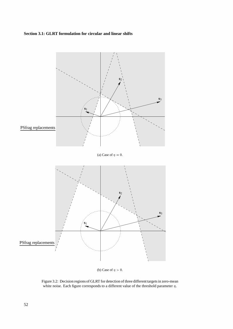
Section 3.1: GLRT formulation for circular and linear shifts
PSfrag replacements
s1
s2
s3
(a) Case of η = 0.
PSfrag replacements
s1
s2
s3
(b) Case of η > 0.
Figure 3.2: Decision regions of GLRT for detection of three different targets in zero-meanwhite noise. Each figure corresponds to a different value of the threshold parameter η.
52
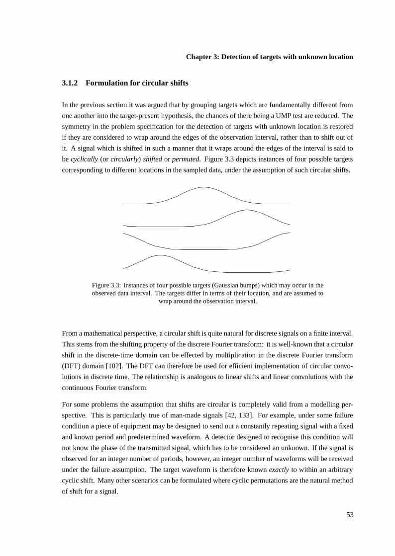
Chapter 3: Detection of targets with unknown location
3.1.2 Formulation for circular shifts
In the previous section it was argued that by grouping targets which are fundamentally different from
one another into the target-present hypothesis, the chances of there being a UMP test are reduced. The
symmetry in the problem specification for the detection of targets with unknown location is restored
if they are considered to wrap around the edges of the observation interval, rather than to shift out of
it. A signal which is shifted in such a manner that it wraps around the edges of the interval is said to
be cyclically (or circularly) shifted or permuted. Figure 3.3 depicts instances of four possible targets
corresponding to different locations in the sampled data, under the assumption of such circular shifts.
Figure 3.3: Instances of four possible targets (Gaussian bumps) which may occur in theobserved data interval. The targets differ in terms of their location, and are assumed to
wrap around the observation interval.
From a mathematical perspective, a circular shift is quite natural for discrete signals on a finite interval.
This stems from the shifting property of the discrete Fourier transform: it is well-known that a circular
shift in the discrete-time domain can be effected by multiplication in the discrete Fourier transform
(DFT) domain [102]. The DFT can therefore be used for efficient implementation of circular convo-
lutions in discrete time. The relationship is analogous to linear shifts and linear convolutions with the
continuous Fourier transform.
For some problems the assumption that shifts are circular is completely valid from a modelling per-
spective. This is particularly true of man-made signals [42, 133]. For example, under some failure
condition a piece of equipment may be designed to send out a constantly repeating signal with a fixed
and known period and predetermined waveform. A detector designed to recognise this condition will
not know the phase of the transmitted signal, which has to be considered an unknown. If the signal is
observed for an integer number of periods, however, an integer number of waveforms will be received
under the failure assumption. The target waveform is therefore known exactly to within an arbitrary
cyclic shift. Many other scenarios can be formulated where cyclic permutations are the natural method
of shift for a signal.
53
Section 3.1: GLRT formulation for circular and linear shifts
In this section the GLRT is derived for the detection problem where the target is known only to within
some cyclic permutation. Again the assumption is made that the noise is additive and multivariate
normal. In principle the test is exactly the same as for the linear shift case, with the set of candidate
targets taken to be cyclically-permuted versions of a prototype target. However, the equations can be
simplified somewhat by introducing notation which is specific to the cyclic case.
Continuing with the formal development, if the prototype target is the n-dimensional vector s then it
is assumed that the possible targets which may be present are s0, . . . , sn−1, where
sθ = Pθs, (3.3)
and P is the cyclic permutation matrix, with
P =
0 · · · 0 1
1 · · · 0 0...
. . ....
...
0 · · · 1 0
. (3.4)
This matrix has the property that premultiplying the column vector s by P cyclically permutes the
elements one position downwards:
Ps =
0 · · · 0 1
1 · · · 0 0...
. . ....
...
0 · · · 1 0
s1...
sn−1
sn
=
sn
s1...
sn−1
. (3.5)
Therefore premultiplying by the matrix Pθ will result in a circular shift downwards by θ positions. Note
that this transformation is reversible, so the matrix P is invertible. Thus it makes sense to consider the
matrix Pθ for θ negative, which will just effect a cyclic shift of a premultiplied vector by |θ | positions
upwards. Furthermore, if s is n-dimensional then the vector Pns, which has been cyclically permuted
n times, will be identical to s.
If it is required to detect instances of such cyclically-permuted targets in MVN noise with mean m and
covariance C, the GLRT is essentially the same as that of the previous section. However, there are now
considered to be n possible targets, corresponding to elements of the set {P0s, . . . , Pn−1s}. Although
cyclic shifts of greater than n positions are possible, they do not result in any new targets. Therefore
the GLRT can be written as
tGLRT(x) = maxθ∈[0,n−1]
{sT P−θC−1(x − m) − 1/2sT P−θC−1Pθs
} H1><H0
η, (3.6)
where use has been made of the property that (Pk)T = Pn−k = P−k . In the event that C is circulant, a
54
Chapter 3: Detection of targets with unknown location
further simplification can be made:
tGLRT(x) = maxθ∈[0,n−1]
{(Pθs)T C−1(x − m) − 1/2sT C−1s
} H1><H0
η. (3.7)
This stems from the result that for C persymmetric (which defines symmetry about the northeast-
southwest diagonal, and is true for both Toeplitz and circulant matrices), the relationship P kCP−k = C
holds for all k [23].
Finally, a special case often of interest is that of detection in white noise, where C = σ 2I. Under these
conditions the test becomes
tGLRT(x) = 1
σ 2max
θ∈[0,n−1]
{(Pθs)T (x − m) − 1
2sT s}
H1><H0
η. (3.8)
The first term on the left of the test inequality is simply the inner product between the observation
x − m and some cyclic permutation of the target s. Furthermore, it is apparent that the statistic
maxθ∈[0,n−1](Pθs)T (x − m) is sufficient for the decision process.
3.1.3 Discussion
In both tests presented, selecting the value of η based on required detection or false alarm rate criteria
generally has to be performed by simulation or by calculations performed on actual data samples, since
the distribution of the test statistic tGLRT(x) does not have a simple closed form. This is true even in
the case of detection in white noise with known variance. The same observation applies in the task of
assessing test performance.
The two tests presented represent different assumptions on the candidate targets which may be consid-
ered present in the observation. Clearly when circular shifts are assumed, the problem formulation no
longer accurately represents a situation where continuous data are sampled and windowed. Nonethe-
less, it can be argued that the differences between the linear and circular shift case are small, particularly
when the observation interval is long and the targets are transient. The differences in the problem spec-
ifications then only occur near the edges of the data interval.
Irrespective of the precise formulation used, a question remains of how good the GLRT solution is
to the unknown target location detection problem. One way of addressing this issue is to compare
the performance of the GLRT to a simple detector which assumes that the target location is precisely
known. This is sometimes referred to as a clairvoyant detector. The comparison then has to be made
for each possible value of the location parameter, since in general the power of the test will differ
for targets at different locations. For all values of θ the detector which “knows” the location of the
possible target will outperform the GLRT, since it is the optimal solution for what then amounts to a
simple hypothesis versus a simple alternative. The comparison is somewhat unreasonable, however,
55
Section 3.2: UMP cyclic permutation invariant detection
since the problem of detection when the target location is known is fundamentally different from that
of the location being unknown.
To make a reasonable assessment of the performance of the GLRT, therefore, an alternative formulation
is required. In the section which follows, it is demonstrated that when the noise has a circulant
covariance matrix (of which white noise is a special case), a uniformly most powerful invariant (UMPI)
test exists for the problem of detecting a target known only to within some arbitrary cyclic permutation.
This test is optimal in the Neyman-Pearson sense out of the class of all tests which are cyclic permutation
invariant. Since the GLRT derived for the same problem is also invariant to cyclic permutations, its
performance is necessarily worse than that of the UMPI test for every value of the unknown location
parameter. By comparing the performance of the two tests it is therefore possible to ascertain the
degree to which the GLRT is suboptimal.
Using this approach the tests may only be compared quantitatively under the assumption that shifts
are circular, and for certain values of the noise covariance matrix. Nevertheless, if the GLRT performs
well under these particular conditions, it may reasonably be expected that it will perform well under
most conditions with shifts defined differently. This conclusion becomes more valid as transient targets
become shorter and observation intervals longer. In essence, insofar as the problems of unknown linear
shifts and unknown cyclic permutations of the target are similar, a comparison under these restricted
conditions can provide an indication of the performance for the related cases.
3.2 UMP cyclic permutation invariant detection
This section presents a derivation of the uniformly most powerful invariant test for detecting a target
which has an arbitrary and unknown cyclic permutation. An invariance condition is imposed on the
testing problem to eliminate the dependence on the unknown shift parameter. The required invariance
that is imposed on the hypothesis test is reasonable for the structure of the problem, so the resulting
optimality is strong. The application of cyclic permutation invariance to the unknown target location
problem appears to be unique, so the derivation is presented in detail.
As with the presentation for the GLRT, it is assumed that n samples of data are observed, represented
by the vector x. Furthermore, it is assumed that any targets which may be present are observed in zero-
mean additive noise with a known circulant covariance matrix — a more general case of the covariance
matrix having certain unknown parameters is discussed in Section 3.4. The noise component n is
therefore assumed to be distributed according to N [0, C], with C circulant. Under hypothesis H0 the
distribution of x is N [0, C]. Under hypothesis H1 some cyclically-permuted version of the prototype
target signal s is added to the noise samples, where the order of the permutation is considered completely
unknown. Thus under H1 the distribution of x is N [Pθ s, C] for some θ . The shift parameter θ is an
unknown deterministic quantity, and without loss of generality can be restricted to take on any integer
56
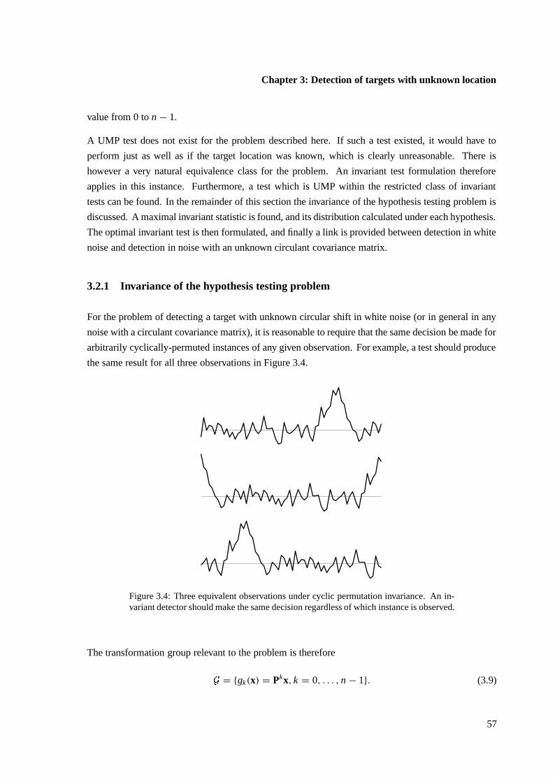
Chapter 3: Detection of targets with unknown location
value from 0 to n − 1.
A UMP test does not exist for the problem described here. If such a test existed, it would have to
perform just as well as if the target location was known, which is clearly unreasonable. There is
however a very natural equivalence class for the problem. An invariant test formulation therefore
applies in this instance. Furthermore, a test which is UMP within the restricted class of invariant
tests can be found. In the remainder of this section the invariance of the hypothesis testing problem is
discussed. A maximal invariant statistic is found, and its distribution calculated under each hypothesis.
The optimal invariant test is then formulated, and finally a link is provided between detection in white
noise and detection in noise with an unknown circulant covariance matrix.
3.2.1 Invariance of the hypothesis testing problem
For the problem of detecting a target with unknown circular shift in white noise (or in general in any
noise with a circulant covariance matrix), it is reasonable to require that the same decision be made for
arbitrarily cyclically-permuted instances of any given observation. For example, a test should produce
the same result for all three observations in Figure 3.4.
Figure 3.4: Three equivalent observations under cyclic permutation invariance. An in-variant detector should make the same decision regardless of which instance is observed.
The transformation group relevant to the problem is therefore
� = {gk(x) = Pkx, k = 0, . . . , n − 1}. (3.9)
57
Section 3.2: UMP cyclic permutation invariant detection
This places an equivalence on the observations {P0x, . . . , Pn−1x}, which is natural on account of
the symmetry of the elements of the observations under each hypothesis. Thus the observations
(x1, . . . , xn−1, xn) ≡ (xn, x1, . . . xn−1) ≡ · · · ≡ (x2, . . . , xn, x1) are all considered equivalent by the
detector. By the way the hypothesis testing problem has been formulated, enforcing this equivalence
is in no way restricting the form of the test.
The testing problem can be seen to be invariant to the group�
. Consider the distribution of the
observation x under each hypothesis: in both cases x is MVN with covariance matrix C. Under H0 the
mean is 0, and under H1 it is one of the elements of the set {P0s, . . . , Pn−1s}. An element gk(x) = Pkx
of the group�
now represents a linear transformation of x. The distribution of y = gk(x) is therefore
N [Pk Ex, PkC(Pk)T ], where Ex is the expected value of x. Noting that (Pk)T = Pn−k = P−k and that
PkCP−k = C for C persymmetric,
y : N [Pk Ex, C]. (3.10)
Thus under H0 the mean of the transformed vector y is 0, and under H1 it is an element of the set
{PkP0s, . . . , PkPn−1s} = {P0s, . . . , Pn−1s}. The transformation gk therefore preserves the form of
the distribution, and retains the partition of the parameter space under each hypothesis. Since this
conclusion applies to all elements g ∈ �, the hypothesis testing problem is invariant-
�.
3.2.2 Maximal invariant statistic for the problem
To find invariant tests, it is useful to find a maximal invariant statistic for the problem. This is a statistic
which has the required invariances, but which also manages to retain the maximum amount of useful
information contained in the observation regarding the decision process. One such statistic can be
obtained by defining Pmax(x) to be that function which cyclically permutes the elements of x until the
element with the maximum value is in the first position of the vector. Note that for the distributions
being considered here Pr{xi = x j} = 0 for i 6= j , so the maximum element of x will be unique with
probability 1.
The statistic Pmax(x) is invariant to the group�
: since one of the elements of x is always maximum
and elements of�
simply permute the observation x cyclically, Pmax[g(x)] = Pmax[x] for all g ∈ �.
Additionally, for the same reasons, the condition Pmax[g(x1)] = Pmax[g(x2)] means that x1 and x2 must
be related to one another through a cyclic shift, so x2 = g(x1) for some g ∈ �. Thus the statistic
Pmax(x) is maximal.
As explained by Lehmann [87] or Scharf [119], the significance of this result is that only functions of
the maximal invariant statistic need to be considered when looking for a test which is invariant to�
.
58
Chapter 3: Detection of targets with unknown location
3.2.3 Distribution of the maximal invariant statistic
The method described by Hogg and Craig [62, p. 142] in relation to order statistics provides a means
of determining the distribution of the maximal invariant. Firstly it is reasserted that two elements of
x are equal with probability zero, so the joint probability density of x can be defined to be zero at all
points which have at least two of their coordinates equal. The set�
where the probability density of
x is nonzero can therefore be partitioned into n mutually disjoint sets:
�1 = {x|x1 = max(x1, . . . , xn)}
... (3.11)�
n = {x|xn = max(x1, . . . , xn)}.
Thus�
i is the set of all points in� n which have no elements equal, and have x i as their largest element.
Consider the function y = Pmax(x). This defines a 1 − 1 transformation of each of�
1, . . . ,�
n onto
the same set � , where it so happens that � = �1. For points in
�i , the transformation y = Pmax(x)
cyclically permutes the elements of x upwards by i − 1 positions. Thus the inverse function is
x = Pi−1y (3.12)
which simply rotates them back downwards by the same amount.
Letting Ji be the determinant of the Jacobian of the inverse transformation corresponding to�
i , it can
be seen that
Ji = |Pi−1|. (3.13)
By the structure of Pi−1, it is always possible to obtain an identity matrix by means of a number of
row exchanges. Thus it must be the case that Ji = +1 or Ji = −1. Denoting the probability density
of x by fx(x), the results of this section can be combined to yield the probability density f y(y) of
y = Pmax(x) [62, p. 143]:
fy(y) =
∑n−1k=0 fx(Pky) y1 = max(y1, . . . , yn)
0 otherwise.(3.14)
This expression can finally be used to find the distribution of the maximal invariant statistic under each
hypothesis. Under H0,
fx(x) = (2π)−n/2|C|−n/2e− 12 xT C−1x. (3.15)
59
Section 3.2: UMP cyclic permutation invariant detection
Therefore the distribution of y = Pmax(x) is
fy(y) =
(2π)−n/2|C|−n/2∑n−1k=0 e− 1
2 (Pky)T C−1(Pky) y1 = max(y1, . . . , yn)
0 otherwise.(3.16)
Once again using the relation (Pk)T = P−k , and noting that if C is persymmetric then C−1 is also
persymmetric, this can be simplified to
fy(y) =
n(2π)−n/2|C|−1/2e− 12 yT C−1y y1 = max(y1, . . . , yn)
0 otherwise.(3.17)
When H1 is in force, the situation is slightly more complex: now the mean of the observation takes
some value in the set {Pθs, θ = 0, . . . , n − 1}. The probability density of x is therefore
fx(x) = (2π)−n/2|C|−1/2e− 12 (x−Pθ s)T C−1(x−Pθ s), (3.18)
where θ is some integer in the range 0 to n − 1. Substituting into the expression for f y(y) gives
fy(y) =
(2π)−n/2|C|−1/2∑n−1k=0 e− 1
2 (Pky−Pθ s)T C−1(Pky−Pθ s) y1 = max(y1, . . . , yn)
0 otherwise.(3.19)
The first case in this expression needs to be looked at in more detail: for the condition y1 =max(y1, . . . , yn),
fy(y) = (2π)−n/2|C|−1/2n−1∑
k=0
e− 12 [Pk(y−Pθ−ks)]T
C−1[Pk(y−Pθ−ks)]
= (2π)−n/2|C|−1/2n−1∑
k=0
e− 12 (y−Pθ−ks)T C−1(y−Pθ−ks), (3.20)
where once again the persymmetry of C has been used. Noting that the summation in this final
expression is over terms corresponding to all unique cyclic permutations of s, it must be the case that
n−1∑
k=0
e− 12 (y−Pθ−ks)T C−1(y−Pθ−ks) =
n−1∑
l=0
e− 12 (y−Pls)T C−1(y−Pls). (3.21)
Thus the density of y under H1 is
fy(y) =
(2π)−n/2|C|−1/2∑n−1l=0 e− 1
2 (y−Pls)T C−1(y−Pls) y1 = max(y1, . . . , yn)
0 otherwise.(3.22)
60

Chapter 3: Detection of targets with unknown location
Finally, a form that is sometimes useful is
fy(y) =
(2π)−n/2|C|−1/2e− 12 (yT C−1y+sT C−1s)∑n−1
l=0 esT C−1P−ly y1 = max(y1, . . . , yn)
0 otherwise,(3.23)
where use has been made of the relation P−lC−1 = C−1P−l .
Under both cases the density of the maximal invariant is independent of the unknown parameter θ . Thus
the unknown permutation parameter has been removed from the problem by the invariance requirement.
3.2.4 Optimal invariant likelihood ratio test
Once the observation x has been mapped onto the corresponding maximal invariant statistic, a simple
likelihood ratio test can be performed on this quantity. The likelihood ratio for the problem is
l(y) = (2π)−n/2|C|−1/2e− 12 (yT C−1y+sT C−1s)∑n−1
l=0 esT C−1P−ly
n(2π)−n/2|C|−1/2e− 12 yT C−1y
= 1
ne− 1
2 sT C−1sn−1∑
l=0
esT C−1P−ly. (3.24)
The log-likelihood ratio is therefore
L(y) = − ln n − 1
2sT C−1s + ln
n−1∑
l=0
esT C−1P−ly. (3.25)
The best invariant test is to compare this ratio to a threshold η, and decide H1 when exceeded:
lnn−1∑
l=0
esT C−1P−ly H1><H0
η + ln n + 1/2sT C−1s. (3.26)
This test is uniformly most powerful out of all tests which share the same invariances. Thus no other
test which is invariant to cyclic permutations of the observations can perform as well, regardless of the
value of the unknown parameter θ . Since the invariance is a perfectly reasonable one for the problem,
the test may be considered optimal.
It is worth noting that the estimation of the parameter θ is explicit in the GLRT of Equation 3.7. Thus
the most likely location of the detected signal is also provided by that test. For the UMPI test, however,
the dependence on the parameter is completely eliminated by the invariance condition. At no point
does this test make use of any estimate of θ , either implicitly or explicitly.
61

Section 3.3: Comparison of GLRT and UMPI tests
3.2.5 Prewhitening in the invariant detection problem
The previous results were based on detection in a zero-mean additive Gaussian noise environment. For
the special case where the noise is white and the elements identically distributed, C = I. In this case
the UMPI test simplifies to
lnn−1∑
l=0
esT P−ly H1><H0
η + ln n + 1/2sT s. (3.27)
It may be observed that the test in Equation 3.26 may be written in the form
lnn−1∑
l=0
esT C−1/2C−1/2P−ly H1><H0
η + ln n + 1/2sT C−1/2C−1/2s
H⇒ lnn−1∑
l=0
e(C−1/2s)T P−l(C−1/2y) H1><H0
η + ln n + 1/2(C−1/2s)T (C−1/2s), (3.28)
where use has been made of both the symmetry and persymmetry of C−1, and the consequent symmetry
and persymmetry of C−1/2. This may be seen to be precisely the test for the case of detection in white
noise given in Equation 3.27, using instead the whitened target C−1/2s and the whitened observation
C−1/2y.
Finally, it is noted that the components of a random vector with a circulant covariance matrix can
be diagonalised by means of the discrete Fourier transform. That is, it is generally possible to find
both C−1/2s and C−1/2y using the DFT. This can provide a fast method of calculating the required test
statistic in the general case of the covariance matrix being circulant.
3.3 Comparison of GLRT and UMPI tests
The UMPI test presented in the previous section is optimal for the problem of detecting targets with
unknown cyclic permutation in noise with zero mean and a known circulant covariance. This condition
is even stronger than that of a stationary constraint, which only requires that the covariance be Toeplitz.
It has been argued that this optimal test for cyclic shifts is useful from the point of view of assessing
the extent to which the GLRT for the same problem is suboptimal. That is, if the GLRT performs well
for the case of cyclic shifts and circulant covariances, then it may be expected to work well for shifts
defined differently and more general covariance structures. No optimal test exists for these cases,
but they are sufficiently similar to the UMPI test problem for general comparisons to apply. This
section therefore presents results which compare the UMPI test performance to that of the GLRT for
the unknown cyclic permutation detection problem.
62
Chapter 3: Detection of targets with unknown location
The UMPI test statistic for the circulant detection problem involves calculating the sum of the elements
of the set {esT C−1P−lx, l = 0, . . . , n − 1}. Each of these elements has a lognormal distribution, since
the exponents are each normally distributed. Furthermore, since the exponents are correlated, the
lognormal elements are dependent on one another.
A closed-form solution does not exist for the distribution of the sum or logarithm of the sum of indepen-
dent lognormally distributed random variables. There is a fair bit of literature on the subject of finding
approximate distributions, however [7]. The standard approach is to assume univariate lognormality
of the sum, and estimate the parameters using a moment or cumulant matching approach [66, 122].
The general case of the lognormal variates being correlated seems similarly intractable, although the
same approaches for approximating the distribution seem to be applicable [54, 1].
For purposes of assessing the performance of the hypothesis test, a problem with this approximation
approach is that it is not certain under which conditions it is valid and accurate. Any apparent insights
gained into the performance of the test therefore have to be confirmed as a matter of course. Fur-
thermore, attempting to determine the conditions under which the approximations apply is not trivial,
particularly with the large number of different combinations of correlations between the elements of
the sum. In the interests of simplicity and accuracy, therefore, the test performance is assessed directly
using statistical simulations.
Similar observations can be made with regard to the distribution of the GLRT statistic. In this case the
component of the test which depends on the observation is given by maxθ∈[0,n−1](Pθs)T C−1x. Under
H0, with x : N [0, C], an assessment of the performance of the GLRT therefore involves finding the
distribution of the maximum of the set of correlated normal random variables. As in the case of the
UMPI test, the distribution of the test statistic has no simple closed form. Once again it therefore seems
reasonable to quantify the performance of the test based on direct simulation.
The required simulations can be performed very efficiently on account of the fact that the primary
components of the detection statistic may be calculated using the DFT. It is therefore possible to make
performance assessments based on large numbers of generated samples, ensuring accurate results.
The remainder of this section provides a comparison between the GLRT and the UMPI tests for the
problem of detecting the basic targets shown in Figure 3.5. Various scalings of these targets are
considered, corresponding to energies of 2, 4, and 8. In all cases, the additive noise is comprised of 64
uncorrelated samples of zero-mean Gaussian noise with unit variance. In terms of method, there is no
loss of generality in assuming uncorrelated noise, since the prewhitening transformation may always
be used to cast the problem into this form. In that case all that is required is to modify the target signal
to be analysed.
Figure 3.6 shows distributions for each of the test statistics for the specific case of the targets of energy
8. In each case the distribution to the right corresponds to H1. These histograms were generated
63

Section 3.3: Comparison of GLRT and UMPI tests
0 10 20 30 40 50 600
0.1
0.2
0.3
0.4
0.5
0.6
0.7
0.8Target 1Target 2Target 3
Figure 3.5: Unit energy test targets used in Monte-Carlo simulations: the targets aresampled Gaussian functions centred on 32, with standard deviations of 1, 4, and 8.
using 25000 noise samples under each hypothesis and 50 bins. Note that the curve styles in the plot
correspond directly to those used for plotting each of the targets in Figure 3.5.
The test performance is not apparent from the histogram plots under the various hypotheses. To
demonstrate this information, Figure 3.7 shows receiver operating characteristic (ROC) curves for the
various target detection scenarios. The first plot demonstrates the relative performance of the two tests
for the three targets in Figure 3.5, under the condition that they have been scaled to have an energy of 2.
The remaining two plots show similar results for targets scaled to have energies of 4 and 8 respectively.
Since the GLRT and UMPI test are both invariant to cyclic permutations and the latter is UMP in this
class, it exhibits uniformly better performance than the GLRT in all cases.
It is clear from the plots that the difference in performance between the tests is marginal for the cases
which were analysed. A closer inspection of the results indicates that the difference does however
depend on the properties of the target being detected:
• The difference in performance between the GLRT and the UMPI test becomes smaller when the
energy of the target to be detected becomes higher. This may be attributed to the fact that the
target location estimate used in the GLRT improves under these conditions, resulting in better
relative performance.
• The difference becomes smaller as the targets become less localised. That is, the performance
of the GLRT is better relative to the UMPI test for the case of detecting target 3 in Figure 3.5
than for target 1. A possible explanation is that for the wider targets the location estimate used
in the GLRT is less important, with errors having less effect on the overall test.
On the whole, the suboptimal GLRT performs exceedingly well for the specific detection problems
analysed. The conclusion that may be drawn is that the GLRT is effective for dealing with the problem
64
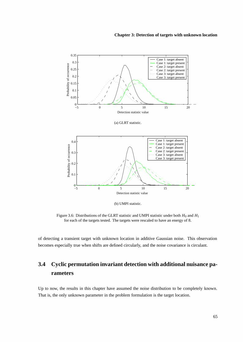
Chapter 3: Detection of targets with unknown location
−5 0 5 10 15 200
0.05
0.1
0.15
0.2
0.25
0.3
0.35
Detection statistic value
Pro
babi
lity
of o
ccur
renc
e Case 1: target absent Case 1: target presentCase 2: target absent Case 2: target presentCase 3: target absent Case 3: target present
(a) GLRT statistic.
−5 0 5 10 15 200
0.1
0.2
0.3
0.4
Detection statistic value
Pro
babi
lity
of o
ccur
renc
e Case 1: target absent Case 1: target presentCase 2: target absent Case 2: target presentCase 3: target absent Case 3: target present
(b) UMPI statistic.
Figure 3.6: Distributions of the GLRT statistic and UMPI statistic under both H0 and H1for each of the targets tested. The targets were rescaled to have an energy of 8.
of detecting a transient target with unknown location in additive Gaussian noise. This observation
becomes especially true when shifts are defined circularly, and the noise covariance is circulant.
3.4 Cyclic permutation invariant detection with additional nuisance pa-
rameters
Up to now, the results in this chapter have assumed the noise distribution to be completely known.
That is, the only unknown parameter in the problem formulation is the target location.
65

Section 3.4: Cyclic permutation invariant detection with additional nuisance parameters
0 0.1 0.2 0.3 0.4 0.5 0.6 0.7 0.8 0.9 10
0.2
0.4
0.6
0.8
1
False alarm probability
Det
ectio
n pr
obab
ility
GLRT: target 1UMPI: target 1GLRT: target 2UMPI: target 2GLRT: target 3UMPI: target 3
(a) Case 1: Targets of energy 2.
0 0.1 0.2 0.3 0.4 0.5 0.6 0.7 0.8 0.9 10
0.2
0.4
0.6
0.8
1
False alarm probability
Det
ectio
n pr
obab
ility
GLRT: target 1UMPI: target 1GLRT: target 2UMPI: target 2GLRT: target 3UMPI: target 3
(b) Case 2: Targets of energy 4.
0 0.1 0.2 0.3 0.4 0.5 0.6 0.7 0.8 0.9 10
0.2
0.4
0.6
0.8
1
False alarm probability
Det
ectio
n pr
obab
ility
GLRT: target 1UMPI: target 1GLRT: target 2UMPI: target 2GLRT: target 3UMPI: target 3
(c) Case 3: Targets of energy 8.
Figure 3.7: ROC curves for detection of the test targets scaled to have energies of 2, 4,and 8.
66
Chapter 3: Detection of targets with unknown location
Often there may be other nuisance parameters defining the noise process. These parameters have to be
dealt with by the test, usually through some estimation procedure. The GLRT, for example, estimates
all the unknown parameters under each assumed hypothesis by maximising the associated likelihood.
The likelihood ratio is then taken to be the ratio of the maximised likelihood under each hypothesis.
In general the nuisance parameter estimates will be different under each assumed hypothesis.
The results of the previous section demonstrate that instead of estimating unknown parameters, it may
be more effective to eliminate them from the problem using an appropriate and sensible invariance
criterion. For the specific cases discussed, the resulting test has a greater power, and is therefore
preferable. In this section the invariance approach is extended to the case where additional unknown
parameters are present in the distributions.
In general it will not be possible to eliminate all nuisance parameters by imposing absolutely reasonable
equivalence classes onto a problem. However, some of the parameters may still be dealt with in this
manner. For example, if it is required to detect targets with unknown location in white noise with
unknown power, the location parameter may still reasonably be eliminated by requiring invariance to
cyclic permutations, as discussed in the previous section. The noise power represents an unknown
parameter which is not removed by the invariance condition, however, and some alternative method of
dealing with it has to be adopted.
The invariant hypothesis testing framework introduces the possibility of making invariant estimates
of these remaining nuisance parameters under each hypothesis. That is, estimates are used which
are invariant to the same group of transformations that have been deemed reasonable for the testing
problem. The reason for requiring this is so that the resulting test is indeed invariant to the group
operation. One way of arriving at such estimates is to find the parameter values that maximise the
likelihood function of the maximal invariant statistic under each hypothesis. Because these estimates
are based on the maximal invariant, they are clearly invariant to the required transformation group.
Additionally, because of the maximality property of this statistic, as much valid information as possible
regarding the unknown parameters is incorporated into the statistic.
In practice, if such invariant maximum likelihood estimates are used, then the resulting test is equivalent
to performing the GLRT on the maximal invariant statistic. The distribution of this statistic may already
be independent of some of the nuisance parameters (through the action of the invariance class), but in
general it may still depend on other unknowns. Formally, suppose an invariant problem formulation
admits a maximal invariant statistic y, which has a density p H0(y|θ0) under H0 and pH1(y|θ 1) under
H1. The parameters θ 0 are those parameters which are not eliminated from the distribution of y under
H0, and θ1 are the parameters which remain under H1. If each of the parameter vectors are permitted
to take on values in the sets 20 and 21 under the two respective hypotheses, then the invariant GLRT
is given by
l(y) = maxθ1∈21 pH1(y|θ1)
maxθ0∈20 pH0(y|θ0)
H1><H0
η. (3.29)
67

Section 3.4: Cyclic permutation invariant detection with additional nuisance parameters
The invariant maximum likelihood estimates of the nuisance parameters under each hypothesis are
those values that maximise each invariant likelihood function.
Any estimate which is based purely on the value of the maximal invariant statistic is guaranteed
to be invariant. Thus the use of maximum likelihood estimates represents only one possibility of
many. In principle, any preferred nuisance parameter estimate could be made, and substituted into the
relevant invariant likelihood ratio. The maximum likelihood estimates, however, are convenient from
a computational perspective, and from the point of view of detection are familiar from the role they
play in the GLRT.
In the section which follows, details of an invariant formulation are presented for the problem of
detecting a known target with unknown circular shift in certain instances of parametrically-known
noise. The unknown location parameter is effectively eliminated by requiring cyclic permutation
invariance in the solution. The covariance matrix of the noise is assumed to be circulant, but depends
on unknown parameters which have to be dealt with by the test. These parameters are estimated by
maximising the invariant likelihood function of the maximal invariant statistic under each hypothesis.
The specific case of the noise covariance being some unknown scaling of the identity matrix is then
discussed in detail. It is demonstrated that cyclic permutation invariant estimates of the unknown noise
power can be made under each hypothesis, by maximising the related invariant likelihood functions.
The ratio of the likelihood values taken on by these functions then constitutes an invariant test statistic,
which can be compared to a threshold in the usual manner. Finally, the performance of this resulting
test is compared to the standard GLRT for the problem, where both the location parameter and the
noise power are assumed unknown, and no invariance condition is imposed.
3.4.1 Invariant estimation of certain circulant covariance matrices
In this section the equations determining the cyclic permutation invariant maximum likelihood estimate
are derived for the problem of estimating unknown covariance matrix parameters. As with the invariant
detection problem, for the invariant formulation to apply the problem has to exhibit some specific
structure. It is therefore assumed that the covariance matrix is circulant, although some of its parameters
are unknown.
If C is full-rank and positive definite, then it can always be expressed in the form C = A6AT , where
A is unitary, and 6 diagonal and positive definite. A special property of circulant matrices is that this
decomposition may always be performed using the same matrix A, and in Chapter 5 it is shown that
for the complex case A may be taken to be the unitary DFT matrix. Thus there exists a known matrix
A such that AT CA is diagonal for every circulant C of interest.
A sample x from an assumed N [Pθ s, C] process is available on which to base the covariance estimate.
68
Chapter 3: Detection of targets with unknown location
As explained, the covariance matrix C depends on certain unknown parameters. The class of problems
considered here involves the case where the unknown parameters of C may be expressed directly
in terms of the diagonal elements of AT CA = 6. In this instance, C is completely specified by
the diagonal elements of 6 = diag(σ 21 , . . . , σ 2
n ), so C may be considered to be a function of these
elements.
The covariance parameter estimate is required to be invariant to the group of transformations�
de-
fined in Equation 3.9, namely that of cyclic permutations of the elements of the observation vec-
tor. As shown in Section 3.2.3, the vector y = Pmax(x) is a maximal invariant for this class, and if
N [Pθ s, C(σ 21 , . . . , σ 2
n )] then
fy(y) = (2π)−n/2|C(σ 21 , . . . , σ 2
n )|−1/2n−1∑
l=0
e− 12 (y−Pls)T C(σ 2
1 ,...,σ 2n )−1(y−Pls) (3.30)
for y1 = max(y1, . . . , yn). The invariant likelihood function under the target present assumption is
therefore given by
L = −n/2 ln(2π) − 1/2 ln |C(σ 21 , . . . , σ 2
n )| + lnn−1∑
l=0
e− 12 (y−Pls)T C(σ 2
1 ,...,σ 2n )−1(y−Pls). (3.31)
Using the decomposition for C and adopting the notation zl = AT (y − Pls), this likelihood may be
written as
L = −n/2 ln(2π) − 1/2 ln |6| + lnn−1∑
l=0
e− 12 (y−Pls)T A6−1A(y−Pls)
= −n/2 ln(2π) − 1/2 lnn∏
k=1
σ 2k + ln
n−1∑
l=0
e− 12 zT
l 6−1zl . (3.32)
Finally, denoting by zl(k) the kth element of the vector zl , this invariant likelihood may be written as
L = −n/2 ln(2π) − 1/2n∑
k=1
ln σ 2k + ln
n−1∑
l=0
e− 1
2
∑nk=1
z2l (k)
σ2k . (3.33)
To arrive at the invariant MLE of the covariance matrix, it is required to maximise this likelihood with
respect to the parameters σ 21 , . . . , σ 2
n , subject to any desired constraints on these elements.
The expression for the invariant likelihood may be maximised under several conditions on the elements
of 6. One case which may be of interest is when all the parameters σ 21 , . . . , σ 2
n are considered unknown
and independent, which corresponds to the assumption that the noise is circulant, but otherwise com-
pletely unknown. A necessary condition on the invariant MLE is then that the derivative d L/dσ 2i be
identically zero for each i , which leads to n simultaneous equations with n unknowns. The equations
69

Section 3.4: Cyclic permutation invariant detection with additional nuisance parameters
are not easily solved, however, since the desired parameters are implicit in the equations.
A simpler case involves the assumption that a sample is provided from a N [Pθ s, σ 2I] process, where
θ and σ 2 are assumed unknown. Through the action of the invariance class, a maximal invariant is
obtained which is independent of θ . However, it is still required to make an invariant estimate of the
parameter σ 2, which parameterises the unknown component of the covariance matrix. It is easy to
see that this scenario corresponds to the choice of A = I in the previous discussion, along with the
condition that σ 21 = · · · = σ 2
n = σ 2 in the diagonalised matrix.
Under these conditions, the invariant likelihood function simplifies to
L = −n
2ln(2π) − n
2ln(σ 2) + ln
n−1∑
l=0
e− 12σ2
∑nk=1 z2
l (k)
= −n
2ln(2π) − n
2ln(σ 2) + ln
n−1∑
l=0
e− 12σ2 zT
l zl . (3.34)
A necessary condition on the invariant maximum likelihood estimate σ 2 of the noise power is that
d L
dσ 2
∣∣∣∣σ 2=σ 2
= 0. (3.35)
This yields the condition
σ 2n−1∑
l=0
e− 12σ2 zT
l zl = 1
n
n−1∑
l=0
zTl zle
− 12σ2 zT
l zl , (3.36)
which can be solved using numerical techniques.
3.4.2 Invariant detection using invariant estimates of nuisance parameters
Once the invariant estimates of the nuisance parameters have been found, they can be substituted
into the invariant likelihood function, and the maximum likelihood value obtained. The ratio of the
maximum likelihood under each assumed hypothesis may then be used as a test statistic.
Consider the case of invariant covariance matrix estimation discussed in the previous section. To use
these estimates in a detector, estimates of C under both the null hypothesis and the alternative are
required. These estimates can be used in the invariant likelihood ratio statistic, which is then given by
t (y) = maxC pH1(y|C)
maxC pH0(y|C), (3.37)
where the maximisation is implied to be over the class of circulant covariance matrices which are
considered valid for the problem. If the invariant maximum likelihood estimates of the covariance are
70
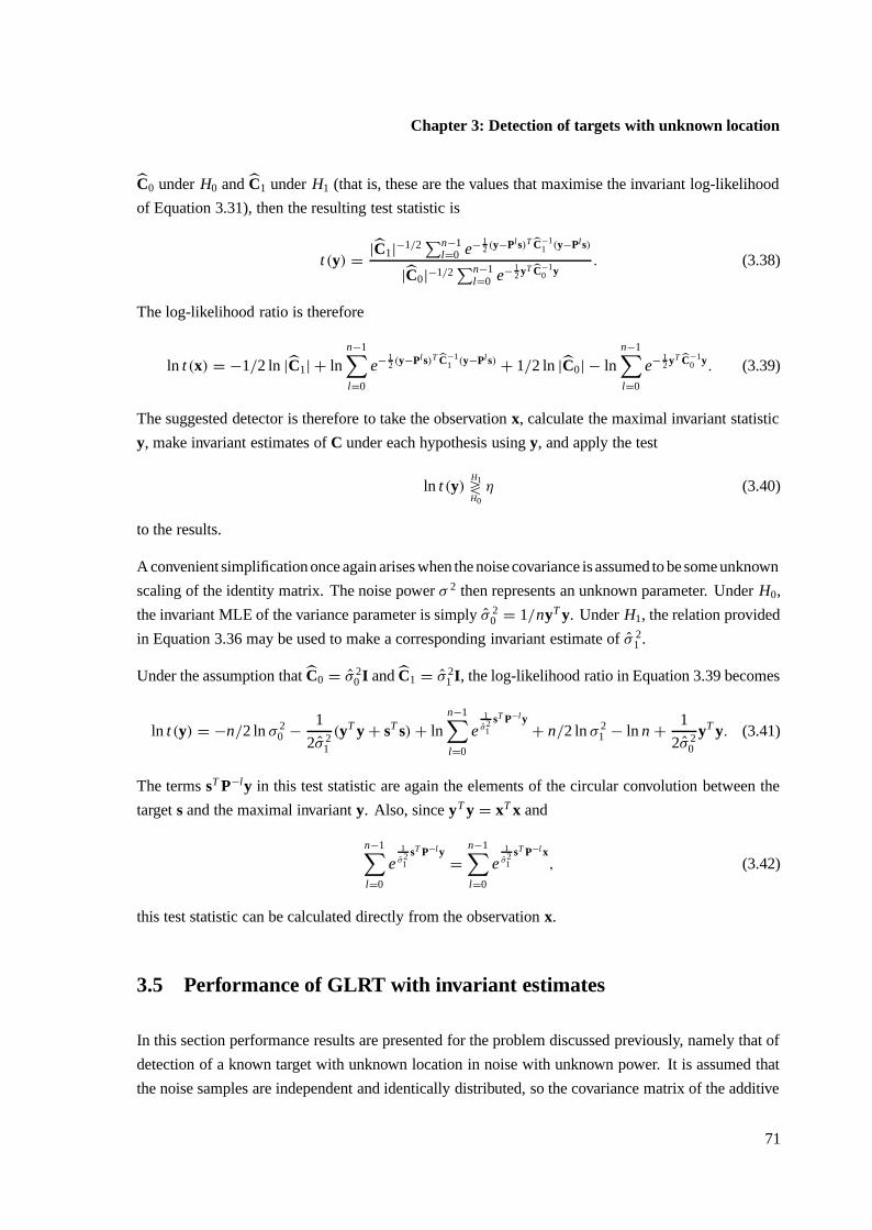
Chapter 3: Detection of targets with unknown location
C0 under H0 and C1 under H1 (that is, these are the values that maximise the invariant log-likelihood
of Equation 3.31), then the resulting test statistic is
t (y) = |C1|−1/2∑n−1
l=0 e− 12 (y−Pls)T C−1
1 (y−Pls)
|C0|−1/2∑n−1
l=0 e− 12 yT C−1
0 y. (3.38)
The log-likelihood ratio is therefore
ln t (x) = −1/2 ln |C1| + lnn−1∑
l=0
e− 12 (y−Pls)T C−1
1 (y−Pls) + 1/2 ln |C0| − lnn−1∑
l=0
e− 12 yT C−1
0 y. (3.39)
The suggested detector is therefore to take the observation x, calculate the maximal invariant statistic
y, make invariant estimates of C under each hypothesis using y, and apply the test
ln t (y)H1><H0
η (3.40)
to the results.
A convenient simplification once again arises when the noise covariance is assumed to be some unknown
scaling of the identity matrix. The noise power σ 2 then represents an unknown parameter. Under H0,
the invariant MLE of the variance parameter is simply σ 20 = 1/nyT y. Under H1, the relation provided
in Equation 3.36 may be used to make a corresponding invariant estimate of σ 21 .
Under the assumption that C0 = σ 20 I and C1 = σ 2
1 I, the log-likelihood ratio in Equation 3.39 becomes
ln t (y) = −n/2 ln σ 20 − 1
2σ 21
(yT y + sT s) + lnn−1∑
l=0
e1
σ21
sT P−ly+ n/2 ln σ 2
1 − ln n + 1
2σ 20
yT y. (3.41)
The terms sT P−ly in this test statistic are again the elements of the circular convolution between the
target s and the maximal invariant y. Also, since yT y = xT x and
n−1∑
l=0
e1
σ21
sT P−ly=
n−1∑
l=0
e1
σ21
sT P−l x, (3.42)
this test statistic can be calculated directly from the observation x.
3.5 Performance of GLRT with invariant estimates
In this section performance results are presented for the problem discussed previously, namely that of
detection of a known target with unknown location in noise with unknown power. It is assumed that
the noise samples are independent and identically distributed, so the covariance matrix of the additive
71
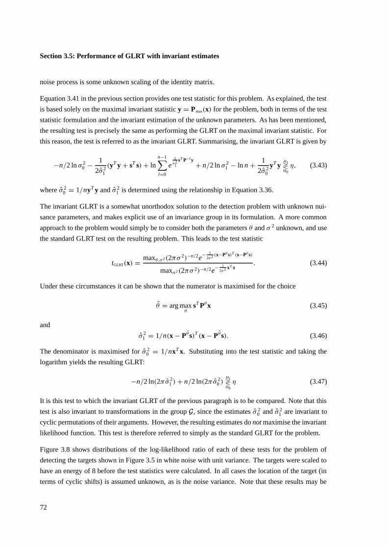
Section 3.5: Performance of GLRT with invariant estimates
noise process is some unknown scaling of the identity matrix.
Equation 3.41 in the previous section provides one test statistic for this problem. As explained, the test
is based solely on the maximal invariant statistic y = Pmax(x) for the problem, both in terms of the test
statistic formulation and the invariant estimation of the unknown parameters. As has been mentioned,
the resulting test is precisely the same as performing the GLRT on the maximal invariant statistic. For
this reason, the test is referred to as the invariant GLRT. Summarising, the invariant GLRT is given by
−n/2 ln σ 20 − 1
2σ 21
(yT y + sT s) + lnn−1∑
l=0
e1
σ21
sT P−ly+ n/2 ln σ 2
1 − ln n + 1
2σ 20
yT yH1><H0
η, (3.43)
where σ 20 = 1/nyT y and σ 2
1 is determined using the relationship in Equation 3.36.
The invariant GLRT is a somewhat unorthodox solution to the detection problem with unknown nui-
sance parameters, and makes explicit use of an invariance group in its formulation. A more common
approach to the problem would simply be to consider both the parameters θ and σ 2 unknown, and use
the standard GLRT test on the resulting problem. This leads to the test statistic
tGLRT(x) = maxθ,σ 2(2πσ 2)−n/2e− 12σ2 (x−Pθ s)T (x−Pθ s)
maxσ 2(2πσ 2)−n/2e− 12σ2 xT x
. (3.44)
Under these circumstances it can be shown that the numerator is maximised for the choice
θ = arg maxθ
sT Pθx (3.45)
and
σ 21 = 1/n(x − Pθs)T (x − Pθs). (3.46)
The denominator is maximised for σ 20 = 1/nxT x. Substituting into the test statistic and taking the
logarithm yields the resulting GLRT:
−n/2 ln(2πσ 21 ) + n/2 ln(2πσ 2
0 )H1><H0
η (3.47)
It is this test to which the invariant GLRT of the previous paragraph is to be compared. Note that this
test is also invariant to transformations in the group�
, since the estimates σ 20 and σ 2
1 are invariant to
cyclic permutations of their arguments. However, the resulting estimates do not maximise the invariant
likelihood function. This test is therefore referred to simply as the standard GLRT for the problem.
Figure 3.8 shows distributions of the log-likelihood ratio of each of these tests for the problem of
detecting the targets shown in Figure 3.5 in white noise with unit variance. The targets were scaled to
have an energy of 8 before the test statistics were calculated. In all cases the location of the target (in
terms of cyclic shifts) is assumed unknown, as is the noise variance. Note that these results may be
72

Chapter 3: Detection of targets with unknown location
compared directly with those of Section 3.3, since the same targets are used and the noise variances
are actually equal. Thus the differences between the results in this section and those of Section 3.3
differ only in that here the noise variance is additionally assumed unknown.
The ROC curves for both the GLRT and the invariant GLRT are shown in Figure 3.9, again for the
targets shown in Figure 3.5. The amplitudes of the targets have been rescaled to result in energies of
2, 4, and 8 for each plot in the figure. In each case the invariant GLRT can be seen to outperform the
standard GLRT, in some cases by quite a significant margin. The difference is more pronounced for
shorter duration targets.
The reason for the better performance of the invariant GLRT relative to that of the standard GLRT can
be attributed to the action of the invariance condition on the problem. The invariance has effectively
eliminated the unknown location parameter, which no longer has to be estimated from the data. This
reduces the uncertainty in the calculated test statistic, thereby improving the performance.
3.6 Concluding remarks
The results of this chapter partially validate the use of the GLRT for detecting targets with unknown
location in noise. For known noise parameters, the detection statistic for this test simply involves
the calculation of the set of inner products {sT1 C−1x, . . . , sT
k C−1x}, where x are the observed data and
s1, . . . , sk are shifted versions of the prototype target which may occur in the data. The GLRT compares
the maximum value of this set to a threshold, and a decision of H1 is made if exceeded.
As shown in this chapter, the GLRT is not optimal for this problem. Unfortunately it is not possible
to assess the extent of its suboptimality for all possible detection cases, but such an assessment can
indeed be made under the assumption of circular shifts and circulant covariances. For this case an
optimal UMPI test can be derived, which is most powerful in the class of all tests which are invariant
to cyclic permutations of the data. When this UMPI test is compared with the GLRT, the performance
difference is seen to be negligible for some common targets.
It must be emphasised that the tests presented are only appropriate for testing the possible presence of
a single target in the observed data. The presence of multiple targets could be dealt with in an ad-hoc
capacity using the proposed tests as a basic structure, but complications may arise if this approach is
adopted. The most serious difficulty in this regard is the estimation of the number and relative location
of targets present, which is required for meaningful detection to take place. A better approach is to
develop explicit models for the multiple target situation, and derive the GLRT accordingly.
For detecting a target with unknown location in a long sequence of data, it is common to slide a
window across the sequence and perform some predetermined detection operation at each point. For
transient targets with limited duration, this results in a set of values which are usually designed to
73
Section 3.6: Concluding remarks
become larger as the likelihood of a target being present increases. The GLRT formulation supports
this implementation method insofar as the test statistic is concerned, although the selection of the
threshold for the test may be nontrivial. This is particularly true if the test threshold is to be obtained
through statistical analysis procedures.
Also demonstrated in this chapter are ways in which an invariance formulation can be applied to de-
tection problems where additional nuisance parameters are present. The use of an invariance subspace
to eliminate some of the parameters has been proposed, with invariant estimates being made of those
parameters which are not eliminated via the invariance condition. It has been shown that even if the
invariance constraint does not eliminate all the parameters, better test performance is nevertheless
obtained through partial parameter elimination. The conclusion may be drawn that if a reasonable
invariance group exists for a problem, then detection performance will benefit by transforming the data
to a maximal invariant. Such a transformation can entirely eliminate unwanted parameters, which then
no longer have to be either estimated or considered any further.
74

Chapter 3: Detection of targets with unknown location
−6 −4 −2 0 2 4 6 8 10 120
0.05
0.1
0.15
0.2
0.25
0.3
Detection statistic value
Pro
babi
lity
of o
ccur
renc
e Case 1: target absent Case 1: target presentCase 2: target absent Case 2: target presentCase 3: target absent Case 3: target present
(a) GLRT statistic.
−6 −4 −2 0 2 4 60
0.1
0.2
0.3
0.4
Detection statistic value
Pro
babi
lity
of o
ccur
renc
e Case 1: target absent Case 1: target presentCase 2: target absent Case 2: target presentCase 3: target absent Case 3: target present
(b) Invariant GLRT statistic.
Figure 3.8: Distributions of the GLRT statistic and invariant GLRT statistic under bothH0 and H1 for each of the targets tested. The targets were rescaled to have an energy of
8.
75
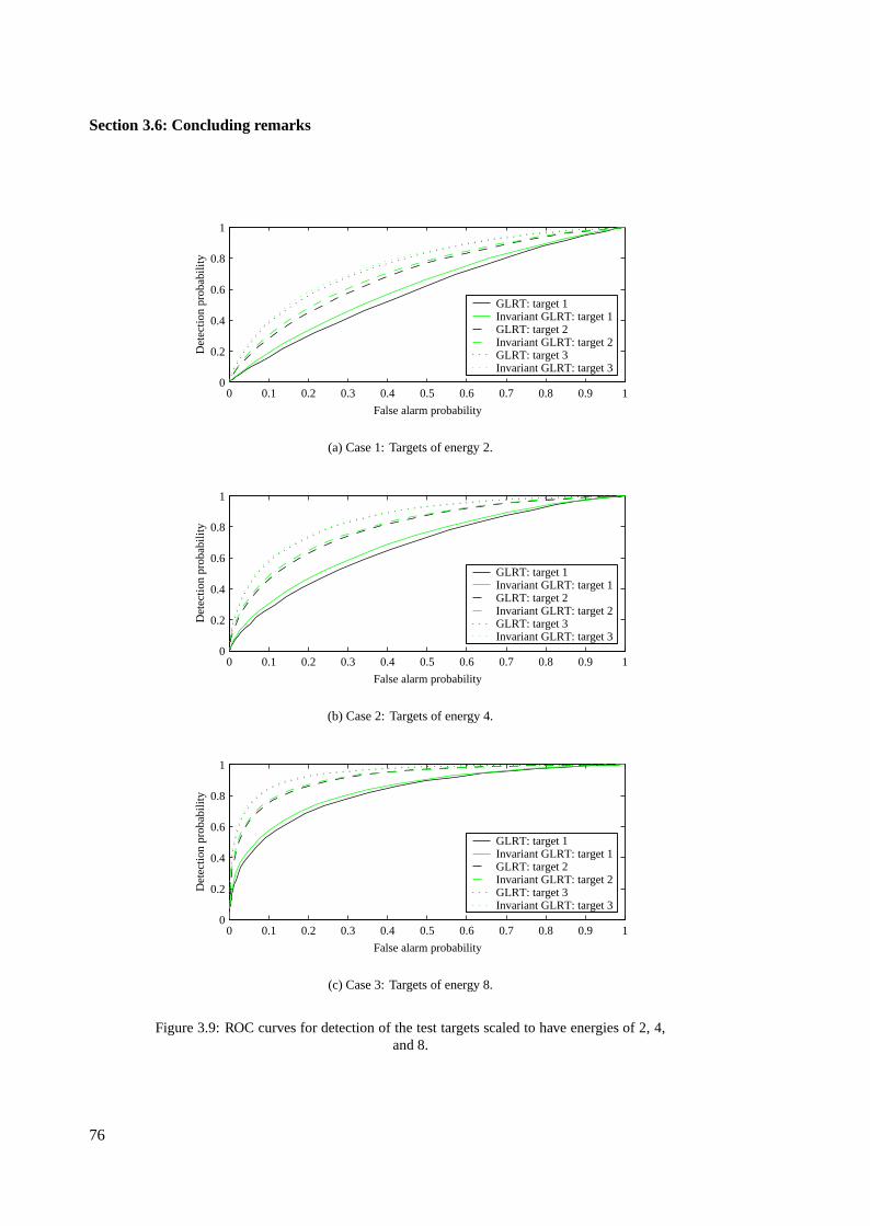
Section 3.6: Concluding remarks
0 0.1 0.2 0.3 0.4 0.5 0.6 0.7 0.8 0.9 10
0.2
0.4
0.6
0.8
1
False alarm probability
Det
ectio
n pr
obab
ility
GLRT: target 1 Invariant GLRT: target 1GLRT: target 2 Invariant GLRT: target 2GLRT: target 3 Invariant GLRT: target 3
(a) Case 1: Targets of energy 2.
0 0.1 0.2 0.3 0.4 0.5 0.6 0.7 0.8 0.9 10
0.2
0.4
0.6
0.8
1
False alarm probability
Det
ectio
n pr
obab
ility
GLRT: target 1 Invariant GLRT: target 1GLRT: target 2 Invariant GLRT: target 2GLRT: target 3 Invariant GLRT: target 3
(b) Case 2: Targets of energy 4.
0 0.1 0.2 0.3 0.4 0.5 0.6 0.7 0.8 0.9 10
0.2
0.4
0.6
0.8
1
False alarm probability
Det
ectio
n pr
obab
ility
GLRT: target 1 Invariant GLRT: target 1GLRT: target 2 Invariant GLRT: target 2GLRT: target 3 Invariant GLRT: target 3
(c) Case 3: Targets of energy 8.
Figure 3.9: ROC curves for detection of the test targets scaled to have energies of 2, 4,and 8.
76

Chapter 4
Subspace invariance in detection
When considering use in practical situations, certain statistical models have significant advantages
over others. These advantages can take the form of easy and convenient model description, efficient
parameter estimation, and closed-form solutions for specific applications.
This is particularly true of the assumption of a Gaussian probability density. It can be specified
using a relatively small number of simple parameters, which are often easily estimated and have well-
documented sampling distributions. The assumption of a normal distribution often leads to linear
models which are completely specified by first- and second-order statistics, resulting in desirable
computational properties.
In some cases it is possible to relax the rigidity of a convenient assumption without completely compro-
mising the resulting simplicity. For example, the autoregressive integrated moving average (ARIMA)
models of Box, Jenkins, and Reinsel [15] extend the validity of conventional ARMA modelling to
nonstationary random signals by means of a simple differencing operation. This presents very little
added complexity in terms of theoretical analysis and practical implementation, but opens up a whole
new range of applications in which ARMA models can be used.
In this section an alternative method of relaxing or extending a preferred statistical characterisation is
presented. The application of the ideas is with regard to simple detection of a known target in noise.
A nominally MVN random process is used for modelling the noise, although in principle the ideas
are not restricted to this case. In particular, the situation is discussed where each noise observation is
assumed to be a realisation of a random process which is only valid within a restricted linear subspace
of the original observation space. The complementary portion of the observation is assumed either to
have been corrupted by unknown interference, to not be conducive to simple statistical modelling, or to
exhibit statistical behaviour that differs from the assumed distribution. Although these situations lead
to identical detectors, the formulations have different statistical justifications and have to be treated
77

separately.
The first case considered is that of subspace interference. Here it is assumed that there is an underlying
process z generating samples on which it is required to perform detection, but that these samples are not
directly observable. Instead, samples of the form x = z + U I c are observed, where c is an unknown
deterministic parameter. Thus there is an additive interference component U I c corrupting the data
observation. It is easy to show that the interference necessarily lies in the subspace 〈U I 〉 spanned by
the columns of UI . This is a linear subspace of the original observation space, and is referred to as the
interference subspace.
A property of the subspace interference formulation is that successive or separate observations are as-
sociated with different values of the interference parameter c. Thus, apart from the subspace constraint,
nothing is known about the interference component.
In Section 4.2 the problem of performing detection in the presence of such interference is discussed.
The paradigm used is that of invariant detection. Because nothing is known about the interference
component for any given observation, it is reasonable to require invariance to these components. It is
demonstrated that within the implied invariance class a uniformly most powerful (UMP) test exists,
which can be claimed to be optimal in the Neyman-Pearson sense.
The use of invariance in dealing with subspace interference is useful for modelling processes which
exhibit statistical predictability, but where low-rank additive contributions are present which may
vary considerably. For example, some time-series processes are almost stationary, but exhibit low-
frequency trends which are sufficient to cast the stationarity assumption in doubt. Rather than trying
to characterise these trends, they may be modelled as subspace interference, thereby eliminating them
from the decision process.
To use the subspace invariant detector in a subspace interference context, it is necessary to identify the
interference subspace. Often this information is provided by peripheral knowledge (such as through
physical modelling of the processes involved), or may be fairly evident just from looking at the data.
However, to be truly useful in a general context some method of identifying interference subspaces
from samples of real data is required.
Section 4.3 deals with this identification for the case where the underlying process (z, as described
above) is multivariate normal with known parameters. A maximum likelihood formulation is presented
for estimating the interference subspace, under the assumption that the rank of the interference is known.
Unfortunately a closed-form general solution has not been found, but a number of approximate methods
are proposed which appear to have merit. Furthermore, exact solutions are provided for two simple
cases. Finally, using statistical simulations, the performance of the estimates are assessed.
The invariant test has application beyond that of detection in subspace interference. In general, subspace
invariance can be used whenever the actual distribution of the data is partially in conflict with some
78
Chapter 4: Subspace invariance in detection
convenient assumed model. Although such a conflict may arise as a result of subspace interference, it
is by no means always the case. In fact, subspace invariant detection can be used in any situation where
mismatch between the data and the model lies mainly within a linear subspace of the original observation
space. Used in this context the detector has no optimality properties. However, the inclusion of an
invariance subspace can reduce model mismatch, thereby improving overall performance.
Section 4.4 discusses this form of invariance in hypothesis testing. Some examples are given of prob-
lems which might benefit from the inclusion of an invariance subspace. From a practical perspective,
the most valuable use of the procedure is in extending the validity of simple or tractable models for
use in situations where they would otherwise be inappropriate.
The problem of identifying candidate invariance subspaces for the model mismatch problem is dis-
cussed in Section 4.5. Since a maximum likelihood solution is difficult to formulate, an alternative
method is developed. In Section 4.5.2 this method is applied to a problem involving real data, and
it is shown that the invariant detector has better detectability and predictability than the noninvariant
detector.
4.1 Linear subspaces
This chapter develops ways in which invariance to linear subspaces can aid in detector performance.
To understand the concepts involved, the notion of a linear subspace has to be understood. This section
provides an overview of the relevant linear algebraic concepts. For a detailed treatment of linear
algebra, the books by Deif [26] and Horn and Johnson [63] are recommended. For a treatment which
is more specific to the subspace invariant detection problem, the introductory chapters of the book by
Scharf [119] should be sufficient.
The notion of an abstract vector space is useful, but is not required in this discussion. Instead, a simpler
vector space can be defined in terms of sets of ordered n-tuples, either with real or complex elements,
that are organised into an n-dimensional vector x = (x1 · · · xn)T . If the elements of x are real, then
we say that x ∈ � n ; if complex, then x ∈ � n . Under the usual definitions of vector addition and
multiplication by a scalar, each of the spaces� n and
� n constitute vector spaces. Considering for
instance the set� n , the assertion follows because the following two properties hold:
x ∈ � n H⇒ ax ∈ � n for any real scalar a, and
x ∈ � n , y ∈ � n H⇒ x + y ∈ � n . (4.1)
Under the circumstances described, these two conditions are all that are required for the set in question
to be a vector space.
79
Section 4.1: Linear subspaces
An important property of a vector space is that it is closed under vector addition and scalar multipli-
cation. Thus these basic operations, when applied to elements of the space, cannot yield a resulting
vector which lies outside of the space.
This closure property of� n and
� n is familiar, and merits no further discussion. Nonetheless, closure
as an abstract concept is useful for defining a subspace of a vector space. Specifically, given a vector
space V , W is a subspace of V if it is contained in V and if it is also closed under vector addition and
scalar multiplication. Thus W is a vector space in its own right, but it is defined in the context of the
larger space V .
A vector space (and therefore a vector subspace) always has a set of linearly independent basis vectors.
The number of vectors in this basis is called the rank or dimension of the space, and is equal to the
minimum number of scalar descriptors needed to uniquely describe an arbitrary point in the space.
Thus if v1, . . . , vn form a basis of� n , then every x ∈ � n can be written as
x = a1v1 + a2v2 + · · · + anvn, (4.2)
for some set of real coefficients a1, . . . , an . Using the basis, every point in� n is therefore associated
with a unique set of n real-valued coefficients.
The basis forms a spanning set of the vector space, since the totality of vectors that can be generated
from the basis (through the operations of vector addition and scalar multiplication) is exactly the vector
space itself. Thus for the real basis v1, . . . , vn described earlier, the set
{a1v1 + a2v2 + · · · + anvn|a1, . . . , an ∈ � } (4.3)
is identically the vector space� n .
Every set of linearly independent vectors spans a linear space. A linear space can therefore be described
in terms of a spanning set of vectors. In this work, the space spanned by the vectors v1, . . . , vk
is represented using the notation 〈v1, . . . , vk〉. If k < n and the component vectors are linearly
independent, then this space will be a k-dimensional subspace of� n , and will be isomorphic to
� k . In
some instances it is convenient to arrange the basis vectors into a matrix
V =(
v1 · · · vk
), (4.4)
in which case the space spanned by the vectors will be denoted by 〈V〉. Every vector of the form Vc
can then be written as
Vc =(
v1 · · · vk
)
c1...
ck
= c1v1 + · · · + ckvk, (4.5)
80
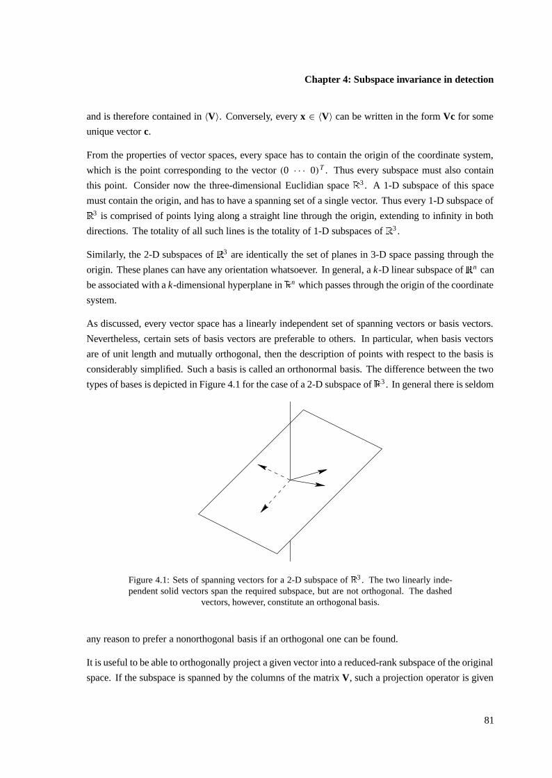
Chapter 4: Subspace invariance in detection
and is therefore contained in 〈V〉. Conversely, every x ∈ 〈V〉 can be written in the form Vc for some
unique vector c.
From the properties of vector spaces, every space has to contain the origin of the coordinate system,
which is the point corresponding to the vector (0 · · · 0)T . Thus every subspace must also contain
this point. Consider now the three-dimensional Euclidian space� 3 . A 1-D subspace of this space
must contain the origin, and has to have a spanning set of a single vector. Thus every 1-D subspace of� 3 is comprised of points lying along a straight line through the origin, extending to infinity in both
directions. The totality of all such lines is the totality of 1-D subspaces of� 3 .
Similarly, the 2-D subspaces of� 3 are identically the set of planes in 3-D space passing through the
origin. These planes can have any orientation whatsoever. In general, a k-D linear subspace of� n can
be associated with a k-dimensional hyperplane in� n which passes through the origin of the coordinate
system.
As discussed, every vector space has a linearly independent set of spanning vectors or basis vectors.
Nevertheless, certain sets of basis vectors are preferable to others. In particular, when basis vectors
are of unit length and mutually orthogonal, then the description of points with respect to the basis is
considerably simplified. Such a basis is called an orthonormal basis. The difference between the two
types of bases is depicted in Figure 4.1 for the case of a 2-D subspace of� 3 . In general there is seldom
Figure 4.1: Sets of spanning vectors for a 2-D subspace of� 3 . The two linearly inde-
pendent solid vectors span the required subspace, but are not orthogonal. The dashedvectors, however, constitute an orthogonal basis.
any reason to prefer a nonorthogonal basis if an orthogonal one can be found.
It is useful to be able to orthogonally project a given vector into a reduced-rank subspace of the original
space. If the subspace is spanned by the columns of the matrix V, such a projection operator is given
81
Section 4.2: Detection in subspace interference
by
PV = V(VT V)−1VT . (4.6)
Since from the form of this operator PV x ∈ 〈V〉 for all x, it is apparent that the range of this transfor-
mation is the required subspace. Additionally, the operator is idempotent, since PV PV = PV . These
two properties are sufficient to define a projection into 〈V〉. That this projection is orthogonal will not
be shown — see [119, p. 46] for details. Finally, if the columns of V constitute an orthogonal basis
for the required subspace, then VT V = I, so PV = VVT yields the required orthogonal projection.
4.2 Detection in subspace interference
This section discusses the problem of detecting a known target in noise which is comprised of two
additive components: a random component from a process with a known probability density, and a
deterministic interference component which is unknown but constrained to lie within a linear subspace
of the observation space. An invariant detector is derived which is optimal in the sense that no other
detector which shares the same invariances can provide better performance. A compelling argument
can therefore be made that this detector is best within the class of all reasonable tests for the problem.
The use of this detector in real situations is outlined, and a form for the test presented which allows
the relevant detector components to be calculated.
Stated formally, each noise observation is assumed to be of the form xi = zi + UI ci , where zi is
a realisation of some N -dimensional random vector with known probability distribution, and c i is a
completely unknown deterministic parameter. The columns of U I are assumed to span the interference
subspace, and may be taken to be orthogonal and of unit length. The interference parameter c i is such
that it differs from one observation to the next, and does not depend on the parameter c j associated
with any other observation x j . Therefore, if multiple samples x1, . . . , xM of noise are observed, then
each sample corresponds to a different value of ci , and the elements of the set c1, . . . , cM do not depend
on one another in any quantifiable manner.
The probability density of the combined noise xi depends on the vector ci , which plays the role of an
unknown deterministic parameter in the problem formulation. This parameter specifies the location
of the distribution: each value of ci corresponds to a probability density function whose location has
been shifted by an amount UI ci . For example, if zi is zero-mean MVN, then xi will have the same
covariance structure, but a mean value equal to U I ci .
Figure 4.2 depicts the case of a 1-D interference subspace with 2-D observations. The dashed contours
represent the distribution of the random component of the noise. Through the action of the interference,
the location of this distribution may be shifted by an arbitrary amount in the direction of the interference
vector i. The solid contours therefore represent one possible density function for the noise-plus-
82
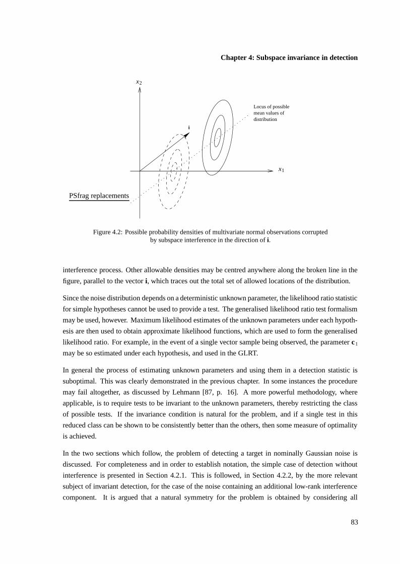
Chapter 4: Subspace invariance in detection
Locus of possiblemean values ofdistribution
i
PSfrag replacements
x1
x2
Figure 4.2: Possible probability densities of multivariate normal observations corruptedby subspace interference in the direction of i.
interference process. Other allowable densities may be centred anywhere along the broken line in the
figure, parallel to the vector i, which traces out the total set of allowed locations of the distribution.
Since the noise distribution depends on a deterministic unknown parameter, the likelihood ratio statistic
for simple hypotheses cannot be used to provide a test. The generalised likelihood ratio test formalism
may be used, however. Maximum likelihood estimates of the unknown parameters under each hypoth-
esis are then used to obtain approximate likelihood functions, which are used to form the generalised
likelihood ratio. For example, in the event of a single vector sample being observed, the parameter c1
may be so estimated under each hypothesis, and used in the GLRT.
In general the process of estimating unknown parameters and using them in a detection statistic is
suboptimal. This was clearly demonstrated in the previous chapter. In some instances the procedure
may fail altogether, as discussed by Lehmann [87, p. 16]. A more powerful methodology, where
applicable, is to require tests to be invariant to the unknown parameters, thereby restricting the class
of possible tests. If the invariance condition is natural for the problem, and if a single test in this
reduced class can be shown to be consistently better than the others, then some measure of optimality
is achieved.
In the two sections which follow, the problem of detecting a target in nominally Gaussian noise is
discussed. For completeness and in order to establish notation, the simple case of detection without
interference is presented in Section 4.2.1. This is followed, in Section 4.2.2, by the more relevant
subject of invariant detection, for the case of the noise containing an additional low-rank interference
component. It is argued that a natural symmetry for the problem is obtained by considering all
83
Section 4.2: Detection in subspace interference
observations which differ by an additive component in the interference subspace to be equivalent.
This leads to the projection of the observation out of the interference subspace as a maximal invariant
statistic, which permits the simple derivation of an optimal invariant test.
4.2.1 Detection without invariance
In the simplest form, the hypotheses are z : N [m0, C] under H0 (the target-absent hypothesis) and
z : N [m1, C] under H1 (the target-present hypothesis). The target to be detected is s = m1 − m0, and
it is assumed that m0, m1, and C are known. For the case of real random vectors, the log-likelihood
ratio for this problem is [119]
L(z) = (m1 − m0)T C−1(z − z0), (4.7)
where z0 = 1/2(m1 + m0). (For the complex case the log-likelihood ratio is L(z) = 2Re{(m1 −m0)
†C−1(z − z0)}, with z0 defined in the same way.) The optimal test is to compare this to a threshold
η, and select H1 when exceeded: that is, choose H1 when
(m1 − m0)T C−1(z − z0) > η. (4.8)
This test is optimal in both the Bayes and the Neyman-Pearson sense, with η chosen accordingly.
Letting wT = (m1 − m0)T C−1, the decision inequality can be written as
wT zH1><H0
η + wT z0, (4.9)
which shows that the inner product wT z is sufficient for the decision process.
It is simple to calculate w for this problem: since wT = (m1 − m0)T C−1 it can be seen that
Cw = m1 − m0, (4.10)
which is just a linear equation with the coefficient matrix being the covariance C. Since C is positive
semidefinite, appropriate algorithms can reduce the complexity of finding a solution [47]. If C is further
known to have a more specific structure, it may be possible to utilise corresponding low-computational
methods. For example, under a stationarity assumption C is symmetric, positive definite, and Toeplitz,
all of which can simplify the calculation of w.
84
Chapter 4: Subspace invariance in detection
4.2.2 Invariant detection for subspace interference
The optimal invariant test is now derived for the problem of detecting a known target s = m1 − m0 in
noise which is essentially MVN but has an additive subspace interference component. It is assumed
that the nominal distribution of the random component of the noise is z : N [0, C], and that the
interference lies in the subspace spanned by U I . The interference subspace is initially assumed known,
as is the covariance matrix C. The invariant detector for this problem has been developed by Scharf
and Friedlander [120], but the derivation is repeated here using a formulation which is more suited to
topics addressed in later sections.
The method used in developing the test is that of invariant testing, as presented by Lehmann [87, p.
282] and Scharf [119, p. 127]: a group of transformations is proposed which are deemed natural
for the problem, under which any reasonable test should be invariant. It is shown that the hypothesis
testing problem is invariant under this group, and a maximal invariant statistic is found. This maximal
invariant statistic is invariant to the required group of transformations, while at the same time retaining
as much valid information regarding the hypothesis in force as possible. Using this statistic, the most
powerful invariant test for the problem is derived. Insofar as the equivalence class implied by the
transformation group is reasonable, the resulting test is optimal.
Continuing with the development, it is assumed that the vector x = z + U I c is observed. The
interference component UI c of this observation depends on the unknown deterministic vector c, and
on the known matrix UI . Under the noise-only hypothesis the distribution of the random component z
is N [0, C], and under the target-present hypothesis z : N [s, C]. It is required to test between the two
hypotheses.
Figure 4.3 demonstrates the structure of the problem for a two-dimensional observation space. Under
H0, the mean of the distribution lies somewhere along the line x = iα, where i spans the interference
subspace. Under H1, the mean lies on the line x = s + iα. In both cases the covariance matrix of the
observation is C.
Since the observed data vectors have been corrupted by low-rank subspace interference, it is reasonable
to require the detector to be invariant to additive contributions within the subspace. This follows since,
in accordance with the assumptions made, the component of the observation that lies in 〈U I 〉 can take on
any value whatsoever. The invariance group is therefore {ga : ga(x) = x + UI a, a ∈ � p }. This places
an equivalence on x and the observation x + U I a, for every choice of a. Enforcing this requirement on
the test is not unreasonable, and should in no way compromise the solution. Figure 4.4 demonstrates
the equivalences dictated by this transformation group for a simple two-dimensional case.
The partition of the problem into relevant subspaces is best demonstrated by expressing the quantities in
the transformed coordinate system spanned by the unitary matrix (U H UI ), where 〈UI 〉 is the invariance
subspace and UH spans the complementary subspace. Under this representation the observed data are
85

Section 4.2: Detection in subspace interference
s
Mean under Mean under
PSfrag replacements
x1
x2H0 H1
x = αi
x = µs + αi
Figure 4.3: Structure of problem for detecting a known target s in MVN noise plussubspace interference. The interference is assumed to be in the direction of the vector i.
The distributions shown are just one instance of many possible combinations.
to be equivalent
Observations anywhere along lines
i
parallel to this one are considered
PSfrag replacementsx1
x2
Figure 4.4: Set of equivalent observations under the assumption that subspace interferencemay be present in the direction of i.
86
Chapter 4: Subspace invariance in detection
(UH UI )T x, so
(UH UI )T x =
(UT
H x
UTI x
)=(
UTH(z + UI c)
UTI (z + UI c)
)=(
UTH z
UTI z + c
). (4.11)
The first component of this vector describes the data in the subspace 〈U H 〉, and the second the data
in the complementary subspace 〈U I 〉. Now, since c can take on any value, the final component of
the transformed vector can take on any value. There is therefore no useful data contained in this
component, and the subspace 〈U I 〉 is useless for inference. It makes sense to require that a detector
not make use of data contained in this subspace.
The invariant detection problem is readily solved in the original observation space, but more insight
is provided if the problem is addressed using the alternative representation just provided. Without
changing the decision problem, the unitary transformation v = (U H UI )T x is therefore made. In this
transformed coordinate system the hypotheses are
H0 : v : N
[(UT
H m0
UTI m0 + c
),
(UT
H CUH UTH CUI
UTI CUH UT
I CUI
)], and
H1 : v : N
[(UT
H m1
UTI m1 + c
),
(UT
H CUH UTH CUI
UTI CUH UT
I CUI
)]. (4.12)
Invariance is required to the unknown parameter c, which can be attained using the group
� ={
ga : ga(v) = v +(
0
a
), a ∈ � p
}. (4.13)
This is a reasonable requirement for the testing problem, and corresponds exactly to the previously
specified invariance group in the original coordinate system.
The transformed hypothesis testing problem is invariant-�
: under H0, for example, the distribution of
ga(v) is
v : N
[(UT
H m0
UTI m0 + c + a
),
(UT
H CUH UTH CUI
UTI CUH UT
I CUI
)], (4.14)
which is still an element of the set of valid distributions of v under H0. The same assertion can be
made for the distribution of the transformed observation under H1.
A maximal invariant statistic for a group�
is a statistic which is invariant to each element of the group,
and which has the added property that the mapping of each equivalence class (as defined by the group
operation) to the statistic value is one-to-one. As described by Lehmann [87], for purposes of invariant
hypothesis testing it is a sufficient statistic. For the problem described here, the maximal invariant
is simply the component of the observation which is not associated with the interference subspace.
87
Section 4.2: Detection in subspace interference
That is, letting v = (pT qT )T with the dimension of q the same as that of the interference subspace,
M(v) = p is a maximal invariant:
• Invariant:
M[ga(v)] = M
[ga
(p
q
)]= M
[(p
q + a
)]= p = M[v]. (4.15)
• Maximal:
M[v(1)] = M[v(2)] H⇒ v(1) = v(2), (4.16)
so
v(1) = v(2) +(
0
a
)= ga(v(2)) for ga(v) = v +
(0
a
)(4.17)
and a = q(1) − q(2).
Since this statistic is sufficient for the invariant hypothesis testing problem, the most powerful invariant
decision rule depends only on M(v) = UTH x = UT
H z. This quantity is N [UTH m0, UT
H CUH ] under H0
and N [UTH m1, UT
H CUH ] under H1. The decision rule resulting from just observing this maximal
invariant statistic value is to choose H1 when
(UTH m1 − UT
H m0)T (UT
H CUH)−1(UTH z − UT
H z0) > η, (4.18)
or equivalently, when
(m1 − m0)T UH(UT
H CUH)−1UTH(z − z0) > η, (4.19)
where z0 = 1/2(m1 + m0). This is the LRT for the maximal invariant, and is therefore most powerful
in the class of all tests invariant to unknown additive interference in 〈U I 〉.
By defining
w = UH(UTH CUH)−1UT
H(m1 − m0), (4.20)
the decision process becomes choosing H1 when
wT z > η + wT z0. (4.21)
It is less obvious how to find the vector w for this case than for the noninvariant case. However, the
following method provides a solution. Let UT = (UH UI )T , and let
A =(
A11 A12
A21 A22
)(4.22)
88
Chapter 4: Subspace invariance in detection
be the inverse of the partitioned matrix
C = UT CU =(
UTH CUH UT
H CUI
UTI CUH UT
I CUI
)=(
C11 C12
C21 C22
). (4.23)
Then, since U is unitary, U−1 = UT and C−1 = UT C−1U. Thus
A =(
UTH C−1UH UT
H C−1UI
UTI C−1UH UT
I C−1UI
). (4.24)
Expanding the identity CA = I and performing some manipulation on the result, it can be shown that
C−111 = A11 − A12A−1
22 A21, (4.25)
from which the following relation results:
(UTH CUH)−1 = UT
H C−1UH − UTH C−1UI (UT
I C−1UI )−1UT
I C−1UH . (4.26)
Noting that UH UTH = I − UI UT
I , we can form the product
UH(UTH CUH)−1UT
H = (I − UI UTI )[C−1 − C−1UI (UT
I C−1UI )−1UT
I C−1] (I − UI UTI ), (4.27)
which simplifies to
UH(UTH CUH)−1UT
H = C−1 − C−1UI (UTI C−1UI )
−1UTI C−1. (4.28)
Substituting into equation 4.20 gives
w = C−1(m1 − m0) − C−1UI (UTI C−1UI )
−1UTI C−1(m1 − m0), (4.29)
which is a function of the terms C−1(m1 − m0) and C−1UI . If UI has a small number of columns
with respect to UH , both of these terms can be calculated as solutions to a set of linear equations,
eliminating the need to calculate C−1. Note that it is at no stage required to specify UH explicitly.
4.2.3 Discussion
The hypothesis test in Equation 4.19 has been shown to be optimal in the class of all tests which are
invariant to arbitrary additive contributions in the interference subspace. This optimality is absolute in
the Neyman-Pearson sense.
89
Section 4.2: Detection in subspace interference
Using Equation 4.28 the test can be written as
(m1 − m0)T C−1(z − z0) − (m1 − m0)
T C−1UI (UTI C−1UI )
−1UTI C−1(z − z0)
H1><H0
η, (4.30)
which is expressed instead in terms of the interference subspace matrix U I . This form is useful for
interpreting the role of the interference subspace. Primarily, the matrix U I can be replaced by UI B
for any invertible B without changing the test. Since under these conditions 〈U I 〉 = 〈UI B〉, the test
depends only on the span of UI , not on the specific choice. This is expected, since the choice of
representation for the interference subspace should not have an effect on the resulting test. Thus the
interference component could just as reasonably be represented by U I Bci , with ci completely unknown.
Since the maximal invariant simply projects the data out of the interference subspace, the details of
the subspace representation have no effect on the ultimate detection.
With regard to invariant hypothesis tests, the equivalences imposed on the observations by the transfor-
mation group are paramount in any optimality discussion. If the transformation group is not absolutely
reasonable for the problem, then even if the best invariant test can be found it cannot be claimed to be
optimal: there may exist a test outside of the invariance class which exhibits better performance. For
detection in subspace interference, the transformation group implies equivalence between observations
which differ only by some component in the interference subspace. This equivalence is only reasonable
if absolutely nothing is known about the interference component beyond the subspace constraint. This
is often an unrealistic assumption — most physical systems are at the very least energy-constrained,
and these constraints constitute information regarding the interference contribution. For example,
interferences corresponding to excessively large values of c simply cannot occur in a voltage signal,
since they will imply impossible energy outputs. Requiring invariance to subspace interference is then
questionable, since the invariance condition is too restrictive to be entirely realistic.
For situations where the equivalence class is appropriate, the test given in Equation 4.19 cannot be
improved upon. It is most powerful in the class of all tests which share the same set of equivalences.
As such, it is the uniformly most powerful invariant (UMPI) test, where the specific invariance group
is implied and is taken to be the set�
. The optimality is in terms of the Neyman-Pearson criterion.
Therefore, for a fixed false alarm rate, the UMPI test has the highest detection probability out of all tests
which are invariant-�
. Ferguson [34, p. 143] and Berger [10, p. 237] discuss the topic of invariance
in a Bayesian context, where invariance of the loss function under the transformation group is also
required, but that is not considered here.
For the tests discussed in this section, the only unknown parameters correspond to the contribution of
the observation in the interference subspace. Since the maximal invariant projects the observed data
out of this space, the distribution under each hypothesis is completely known and is independent of any
unknown parameters. It is for this reason that the UMPI test is trivial to find. In general this will not be
the case — the target to be detected may be parameterised by unknowns, and the noise contribution may
90
Chapter 4: Subspace invariance in detection
depend on parameters which are unknown and cannot be eliminated through a reasonable invariance
constraint. If subspace interference is still present in the observation, however, the maximal invariant
statistic continues to play a pivotal role in the formulation of any subsequent test: it contains more data
than any other statistic which is independent of the subspace interference component.
Given a problem where there are unknown parameters in addition to the unknown interference, the
procedure for invariant detection is then to find the maximal invariant statistic, calculate its parametric
distribution under the hypotheses, and address the resulting problem in its own right. For example,
once the maximal invariant has been found, the GLRT may be used on the reduced problem to find a
reasonable test. If a test can be found which is optimal for all values of the unknown parameters, then
once again a UMPI test results. The use of the maximal invariant completely eliminates the problems
associated with the interference, and no useful information has been lost through the transformation.
The importance of the maximal invariant statistic applies to hypothesis testing paradigms outside the
realm of parametric statistical classifiers. For example, ANN classifiers will also benefit from reduc-
tions brought about by invariance arguments, if indeed they are appropriate. The reduced variability
in the data resulting from replacing the original data with the maximal invariant translates directly to
better learning in the classifier: less of the available capacity of the network is wasted on trying to
characterise corrupted data components.
Finally, when used to justify optimality, invariance can only be applied successfully to problems which
exhibit a significant degree of symmetry [88, p. 85]. To place an equivalence class on sets of obser-
vations requires that the problem be entirely symmetric with regard to the associated transformations.
This restricts the applicability of the concept somewhat — most problems do not have sufficient sym-
metry for invariance concepts to be applied to them without effecting a loss in possible performance.
However, for those problems where symmetry does exist, the notion has considerable value.
4.3 Interference subspace estimation for invariant detection
In some applications it may be obvious which subspaces can be associated with interference, and are
therefore candidates for inclusion in the invariance subspace of an invariant detector. For example,
for detection of transients in a voltage signal which is subject to slow drift, it makes sense to require
invariance to DC offset at the very least. That is, components of the observation spanned by the vector
(1 1 · · · 1)T should be ignored in the detection.
The presence of interference may be more subtle, however, and a systematic method of identifying
interference subspaces from samples of target-free data is desirable. In this section a maximum
likelihood formulation is presented for this identification procedure. If this maximum likelihood
estimate is plugged into the test statistic for the invariant detector, the resulting test is not longer
91

Section 4.3: Interference subspace estimation for invariant detection
optimal. Nevertheless, its performance may still be better than a test which ignores the presence of
interference when it is in fact present.
The results of this chapter make the assumption that the actual underlying distribution of the data is
MVN, with known parameters. The dimension of the interference subspace is also assumed known.
An invariant likelihood formulation is developed, which attempts to find an invariance subspace which
has the property that the likelihood of observing the given data in the complementary subspace is
maximised.
For all but the simplest formulations, the mathematical details are complicated and do not lead to
tractable solutions. Some progress can nevertheless be made in general terms, and leads to insights
into the characteristic properties of good invariance subspaces. Additionally, the necessary condition
on the interference subspace estimate can be solved in some special instances, which can be used to
develop approximate solutions for the general case.
The proposed identification method takes no account of the target to be detected. It is conceivable,
therefore, that the estimated interference subspace completely contains a target which it is required
to detect. Invariant detection then becomes impossible, since the valid components of the data are
identical under both hypotheses. This cannot be considered a failing of the identification method,
however: if a target does indeed lie in the interference subspace, then any detector will necessarily
fail. Other advantages of decoupling the interference subspace estimate from the detection problem
are that the noise modelling becomes independent of the target to be detected. This is useful if many
different possible targets can be present in the data, and it is required to detect any single instance of
one of them.
The assumption that the underlying data distribution is known is restrictive, and limits the utility of the
proposed methods in practical problems. However, in Chapter 5 some methods are presented whereby
this requirement is relaxed, and interference subspace estimates can be obtained for models which are
not completely known.
Section 4.3.1 discusses the effect that subspace interference can have on the sample mean and covariance
matrix of corrupted data samples. It is demonstrated that the interference can cause a shifting in the
mean value of the sample distribution from its nominal position. Also, the interference can result in
an increased variance in the directions associated with the interference subspace.
In Section 4.3.2, the invariant likelihood function is presented, which expresses the likelihood of ob-
serving the components of a data sample which lie in the subspace complementary to the interference
subspace. It is this invariant likelihood which it is required to maximise, to obtain the maximum like-
lihood interference subspace estimate. The details of the maximisation are presented, and a necessary
condition on the estimate is obtained.
Section 4.3.3 discusses the solutions to the estimation problem for two special cases. In particular, the
92
Chapter 4: Subspace invariance in detection
case of a white noise assumption on the covariance matrix of the underlying process is considered,
and a closed-form solution is provided for the subspace estimate. The case of the covariance matrix
being completely unknown is also presented: although this strictly belongs in the next chapter, it is
discussed here on account of its similarity to the white noise case.
As mentioned, the necessary condition on the subspace estimate has not been solved for the general
case. Section 4.3.4 therefore discusses an approximate procedure for the estimation, which makes use
of the solution for the white noise case. In short, the observed data are prewhitened using the assumed
known covariance, and the subspace identification performed in this whitened coordinate system.
The estimate is then transformed back into the original coordinates, yielding an approximation to the
required estimate. The accuracy of this procedure increases as the covariance of the data tends to some
scaling of the identity matrix.
Finally, in Section 4.3.6 some results are presented which demonstrate the accuracy of the estimation
procedures for simulated data. Some idea is given of the number of data samples required for the
estimate to be reasonable.
4.3.1 Effect of interference on sample mean and covariance
If the nominal distribution of the data is known or can be accurately assumed, then samples of actual
data can be used to find those subspaces which are most likely to contain interference. To this end,
it is informative to characterise the manner in which interference manifests itself in the sample mean
and sample covariance of the observations. In the remainder of the discussion, the sample covariance
of the realisations x1, . . . , xM is defined to be
Sx x = 1
M
M∑
i=1
(xi − mx)(xi − mx)T , (4.31)
where mx is the sample mean. In some texts the factor 1/(M − 1) is used instead of 1/M , which
results in the sample covariance being an unbiased estimator of the distribution covariance, but this is
not appropriate in a likelihood context.
The mean of a sample of data with interference is given by
mx = 1
M
M∑
i=1
xi , (4.32)
where xi is assumed to be an observation of the form
xi = zi + UI ci , (4.33)
93

Section 4.3: Interference subspace estimation for invariant detection
and the noise-only hypothesis is in force. In terms of the underlying process, this sample mean is equal
to
mx = 1
M
M∑
i=1
(zi + UI ci)
= 1
M
M∑
i=1
zi + UI
(1
M
M∑
i=1
ci
)
= mz + UI mc, (4.34)
where mz = 1/M∑M
i=1 zi and mc = 1/M∑M
i=1 ci . If the mean value of zi is assumed to be m0 and
the covariance matrix C, then taking expectations yields
Emx = m0 + UI mc, (4.35)
so the expected value of the sample mean is the distribution mean of the nominal data samples plus an
unknown offset in the subspace 〈U I 〉.
Using the corrupted data to calculate the sample covariance gives
Sx x = 1
M
M∑
i=1
(xi − mx)(xi − mx)T
= 1
M
M∑
i=1
[(zi + UI ci) − (mz + UI mc)][(zi + UI ci) − (mz + UI mc)]T . (4.36)
Simplifying and noting that E(zi − mz) = 0, the expected value of the sample covariance becomes
E Sx x = E Szz + UI βUTI . (4.37)
Here, β = 1/M∑M
i=1(ci − mc)(ci − mc)T is a symmetric positive semidefinite matrix, which apart
from this condition can take on any values whatsoever.
Apart from the requirement that it be symmetric and positive semidefinite, the matrix β in Equation 4.37
has components which can take on any values. This is because β is the sample covariance of the
unknown components c1, . . . , cM . Since nothing is known about the distribution of ci , the matrix β is
unknown.
The effect of the interference on the expected value of the sample covariance is therefore simply an
94

Chapter 4: Subspace invariance in detection
additive offset of the form UI βUTI . Letting
UI =(
i1 · · · ip
)and β =
β11 · · · β1p...
. . ....
βp1 · · · βpp
, (4.38)
the product UI βUTI expands to
UI βUTI = β11i1iT
1 + β21i2iT1 + · · · + βp1ipiT
1
+ β12i1iT2 + β22i2iT
2 + . . . + βp2ipiT2
+ · · · + β1pi1iTp + β2pi2iT
p + · · · + βppipiTp ,
(4.39)
with β j k = βkj since β is symmetric. Also, since β is positive semidefinite, the coefficients β j j are
nonnegative for all j .
Consider pairs of terms in this sum with coefficients β j k and βkj :
β j k i j iTk + βkj ik iT
j = β j k(i j iTk + ik iT
j ). (4.40)
This sum (which is an n × n matrix) is symmetric since
(i j iTk + ik iT
j )T = i j iT
k + ik iTj . (4.41)
Rearranging and using symmetry, the expected value of the sample covariance of the corrupted obser-
vations is
E Sx x = E Szz + β11i1iT1 + β12(i1iT
2 + i2iT1 ) + · · · + β1p(i1iT
p + ipiT1 )
+ β22i2iT2 + · · · + β2p(i2iT
p + ipiT2 )
+ · · · + βppipiTp
(4.42)
with all the coefficients β j k arbitrary within the constraint that β be nonnegative definite.
Thus the expected value of the sample covariance with interference is the expected value of the sample
covariance without interference, plus a linear combination of terms from the set
{i j iT
k + ik i j ; j, k = 1, 2, . . . , p}, (4.43)
where p is the dimension of the interference subspace. Also, the components i j iTj must have nonneg-
ative coefficients for all j .
By way of example, suppose the interference subspace contributes a constant additive offset with
unknown amplitude to the observations, as well as an additive linear trend with unknown slope. The
95

Section 4.3: Interference subspace estimation for invariant detection
basis vectors for this subspace can be taken to be the vector of ones and a zero-mean vector representing
a linear ramp, both normalised to unit length. These basis vectors are shown in Figure 4.5. Denoting
5 10 15 20 25 30−0.4
−0.2
0
0.2
0.4Basis function 1Basis function 2
Figure 4.5: Basis functions for example 2-D interference subspace.
this first vector by i1 and the second by i2, the presence of interference will shift the location of the
sample mean by c1i1 + c2i2, with c1 and c2 unknown. The sample covariance matrix will contain
additive linear combinations of the form β11i1iT1 +β12(i1iT
2 + i2iT1 )+β22i2iT
2 . These three components
are shown in Figure 4.6. Note that the first and third components must have nonnegative coefficients
Figure 4.6: Components of interference contributions in the sample covariance matrix forcorrupted data. The intensity in these plots is proportional to the value of the components.
in their contribution to the sample covariance. The second can take on any values within the constraint
that the coefficient matrix be nonnegative. Since iTj Sx x i j = iT
j Szzi j + β j j is simply the variance of the
samples in the direction of the vector i j , it is clear that the presence of interference can only increase
the sample covariance in the directions of the basis vectors.
4.3.2 Likelihood function with interference
Suppose the nominal distribution of the noise-only data, before interference has been introduced, is
N [m0, C] with m0 and C known. If the interference lies in the subspace 〈U I 〉 with UTI UI = I, then
the only useful data we have regarding the distribution are samples from the process y = UTH z, where
the columns of UH = (h1 · · · hn−p) are orthonormal basis functions for the sample space of useful
96

Chapter 4: Subspace invariance in detection
data. These are effectively samples from the random process y : N [UTH m0, UT
H CUH ]. This is the
distribution of the data that lies outside the interference subspace.
The estimation proceeds by finding the matrix UH that maximises the likelihood of the observed data
in the subspace 〈UH 〉. The interference subspace estimate is then 〈UI 〉, chosen so that 〈UI 〉 ⊥ 〈UH 〉.
The probability density function for the data y1, . . . , yM is
p(y1, . . . , yM) = (2π)−M(n−p)/2|UTH CUH |−M/2e−1/2
∑Mi=1(yi−UT
H m0)T (UT
H CUH )−1(yi−UTH m0). (4.44)
Thus the log-likelihood is
L y(UH) = K − M
2ln |UT
H CUH | − 1
2
M∑
i=1
(yi − UTH m0)
T (UTH CUH)−1(yi − UT
H m0) (4.45)
which, since yi = UTH zi = UT
H xi , is equal to
L x(UH) = K − M
2ln |UT
H CUH | − 1
2
M∑
i=1
(xi − m0)T UH(UT
H CUH)−1UTH(xi − m0)
= K − M
2ln |UT
H CUH | − M
2
1
M
M∑
i=1
tr{UH(UT
H CUH)−1UH(xi − m0)(xi − m0)T}
= K − M
2ln |UT
H CUH | − M
2tr{UH(UT
H CUH)−1UTH Sx x
}
= K − M
2ln |UT
H CUH | − M
2tr{(UT
H CUH)−1UTH Sx xUH
}. (4.46)
The matrix Sx x = 1/M∑M
i=1(xi − m0)(xi − m0)T is the sample covariance of the data under the
assumption that the mean is known, and equal to m0. For maximum likelihood estimation, it is the
quantity L x which has to be maximised with respect to the choice of UH , subject to the constraint that
UTH UH = I. Note that this is a function of the corrupted data observations x1, . . . , xM .
The requirement that UTH UH = I leads to (n − p) + [(n − p) − 1] + · · · + 1 unique constraints, n − p
of which are (for i = 1, . . . , n − p):
gii(h1, . . . , hn−p) = hTi hi − 1 = 0. (4.47)
The remaining constraints can be written as
g j k(h1, . . . , hn−p) = 2hTj hk = 0, (4.48)
97
Section 4.3: Interference subspace estimation for invariant detection
for j = 1, . . . , n − p and k = j + 1, . . . , n − p. The Lagrangian for the problem is given by
� = − M
2ln |UT
H CUH | − 1
2
M∑
i=1
(xi − m0)T UH (UT
HCUH)−1UTH(xi − m0)
+n−p∑
j=1
n−p∑
k≥ j
λ j kg j k(h1, . . . , hn−p). (4.49)
Necessary conditions for an extremum are that d �dUH
∣∣∣UH =UH
equal the zero matrix. The matrix derivative
of this expression can be found using the results presented in Section 4.6, yielding
d�
dUH= −MCUH(UT
H CUH)−1
− M(I − CUH(UTH CUH)−1UT
H)Sx xUH(UTH CUH)−1 + 2UH0. (4.50)
The necessary condition on the interference subspace estimate UH is therefore
2
MUH0 = CUH(UT
H CUH)−1 + (I − CUH(UTH CUH)−1UT
H)Sx xUH(UTH CUH)−1. (4.51)
Evoking the constraint UTH UH = I and solving for 0 gives
0 = M
2
(I + (UT
H − UTH)Sx xUH(UT
H CUH)−1) = M
2I. (4.52)
Substituting back and postmultiplying by UTH CUH yields the final form of the necessary condition on
the estimate UH to be
UH(UTH CUH) = CUH + Sx xUH − CUH(UT
H CUH)−1UTH Sx xUH . (4.53)
This is a complicated matrix equation in UH . A few things can be said about the nature of the solutions:
• If UH is a solution and R is an orthogonal matrix of the appropriate dimension, then UH R is
also a solution. It is orthogonal, and its columns span the same space as UH . Thus all that can
be ascertained is the space of the columns of UH .
• If UH is multiplied on the left by an orthogonal matrix L, and C is replaced by LCLT and
Sx x by LSx xLT , the problem is unchanged. Since C and Sx x are symmetric, L can be chosen
to diagonalise either of them. Thus either C or Sx x can be assumed diagonal without loss of
generality.
Even with these insights, a closed-form solution to this equation has not been found. Nonetheless, it
can be solved for two special cases, which provides some insight into the nature of the solutions.
98

Chapter 4: Subspace invariance in detection
4.3.3 Specific cases of interference subspace estimation
There are two cases where the estimate of UH which maximises the likelihood has been found. The
first is where the noise model is such that the samples are uncorrelated and identically distributed. The
second occurs when no previous assumptions are made regarding the covariance C, but it is instead
estimated simultaneously from the observed data samples. It is shown in this section that both cases
lead to the same necessary condition on the invariance subspace. A method of finding an orthogonal
basis for the interference subspace estimate 〈UI 〉 is then presented.
Interference subspace estimation for an uncorrelated noise model
The first special case of interest is when the components of the noise vector are uncorrelated and
identically distributed. This corresponds to the condition C = σ 2I, whereσ 2 can be considered a known
or unknown constant. The likelihood function to be maximised then becomes (from Equation 4.46)
L = K − M
2
[n ln σ 2 + tr(UT
H Sx xUH)], (4.54)
so a constrained minimisation of the term tr(UTH Sx xUH) with respect to UH yields the required estimate.
Since the entire problem has been formulated in� n , it is reasonable to require that UH be real.
The necessary condition on the maximum likelihood estimate of the retained subspace in the problem
therefore becomes (from Equation 4.53)
σ 2UH = σ 2UH + Sx xUH − σ 2UH (σ 2)−1UTH Sx xUH , (4.55)
which upon simplification yields
UH UTH Sx xUH = Sx xUH . (4.56)
As with the general condition given in the previous section, the solutions to this equation can also be
seen to be invariant to multiplication on the right by any orthogonal matrix R. Thus all that may be
ascertained is the space of the columns of UH .
The condition on UH implies that
UH UTH Sx xUH w = Sx xUH w (4.57)
for all vectors w, and the converse is also true. Letting v = UH w, as w varies, v takes on all vectors
in 〈UH 〉. Thus the condition can be expressed as follows: for all v ∈ 〈UH 〉,
UH UTH Sx xv = Sx xv. (4.58)
99
Section 4.3: Interference subspace estimation for invariant detection
Additionally, the matrix UH UTH is an idempotent operator which projects orthogonally into the space
〈UH 〉. Thus the implication is that the vector Sx xv must lie in the span of UH .
Bearing in mind that only the space spanned by the columns is specified by the necessary condition,
in the search for solutions UH to Equation 4.56 one is therefore looking for a subspace 〈UH 〉 which
has the property that
∀v ∈ 〈UH 〉, Sx xv ∈ 〈UH 〉 (4.59)
In other words, the vector subspace 〈UH 〉 is mapped into itself by the transformation matrix Sx x .
Equivalently, 〈UH 〉 must be an invariant subspace of the mapping.
Invariant subspaces are discussed by Golub and Van Loan [47, p. 190] and Watkins [129, p. 287],
and from a more algebraic perspective by Gastinel [43, p. 183]. In short, a subspace�
is invariant
to transformation by the matrix A if for every v ∈ �the transformed vector Av ∈ �
. The notion has
particular relevance to numerical computation of matrix eigenvalues and certain other decompositions.
A useful theorem regarding invariant subspaces is provided and proved by Watkins [129, p. 288]:
Let�
be a subspace of � n with basis x1, . . . , xk . Thus� = 〈x1, . . . , xk〉. Let X =
[x1 · · · xk] ∈ � n×k . Then�
is invariant under A ∈ � n×n if and only if there exists
B ∈ � k×k such that AX = XB.
Here � can be any algebraic field, and in particular we may take � = �or � = �
.
Returning to the original minimisation problem, we are attempting to find a real matrix UH which
minimises tr(UTH Sx xUH) subject to the constraint that UT
H UH = I. Furthermore, 〈UH 〉 must be an
invariant subspace of Sx x . We proceed by finding the minimum achievable value of the likelihood
term, and then find a suitable matrix UH which attains this minimum.
Suppose UH ∈ � n×(n−p) spans an invariant subspace of Sx x , and UTH UH = I. Then, by the theorem
given earlier, there exists a matrix B such that Sx xUH = UH B. B can be written as B = G3G−1 for
some diagonal 3 and some invertible G with unit-length columns. Thus Sx xUH G = UH G3. Letting
F = UH G, we note that F also has unit-length columns. With this definition, the previous expression
becomes Sx xF = F3, which is recognised as a standard eigenequation. Thus the diagonal elements of
3 are eigenvalues of Sx x , with the columns of F being the corresponding eigenvectors. Furthermore,
if Sx x is real and symmetric, the eigenvalues and eigenvectors are real.
With this insight, the term tr(UTH Sx xUH) is again considered. Since the columns of UH are orthogonal,
UTH Sx xUH = G3G−1. Thus
tr(UTH Sx xUH) = tr(G3G−1) = tr(3). (4.60)
Since the elements of 3 are eigenvalues of Sx x , this trace can be minimised by choosing F such that its
100
Chapter 4: Subspace invariance in detection
columns are eigenvectors corresponding to the n − p smallest eigenvalues. A solution for UH can now
be found as follows: since the columns of F can always be orthogonalised, there exists an orthogonal
matrix Q and a matrix R such that F = QR (the QR decomposition is one way of finding such an
orthogonal Q). Let UH = QM for M any ((n − p) × (n − p))-dimensional orthogonal matrix. Then
tr(UTH Sx xUH) = tr(MT QT Sx xQM) = tr(QT Sx xQ). (4.61)
Since Sx xQR = QR3, if R is invertible then QT Sx xQ = R3R−1. Thus
tr(QT Sx xQ) = tr(R3R−1) = tr(3), (4.62)
so tr(UTH Sx xUH) attains the minimum at UH = UH .
In summary, then, the required estimate of UH may be found as follows:
• Find the eigenvectors of Sx x corresponding to the (n − p) smallest eigenvalues. Arranging these
eigenvectors into the columns of the matrix F, we have Sx xF = F3.
• Find an orthogonal matrix Q and a matrix R such that F = QR.
• Let UH = QM for any orthogonal M.
The procedure presented here for finding the solution is more general than is required, and charac-
terises the entire class of possible solutions. It is also appropriate in the case where the matrix S x x
is not symmetric, where the eigenvectors are not orthogonal. If just one solution is required and the
assumption of symmetry can be made, then in the previous steps we may always choose R = M = I.
Then the matrix UH may simply be chosen to consist of the eigenvectors corresponding to the (n − p)
smallest eigenvalues of Sx x . UH is then orthogonal, as required, and minimises the likelihood term for
the problem.
Clearly the solution is not unique — postmultiplication by any unitary matrix (or equivalently, rotation
in the subspace spanned by the columns) leaves the likelihood unchanged. If the eigenvalues of S x x
are not unique then even the invariant subspace may not be uniquely specified. In that case there are
multiple maximum likelihood estimates, and one may be selected arbitrarily.
Interference subspace estimation for unknown model covariance
The second special case occurs when the covariance matrix C of the model cannot be specified in
advance. It is then possible to simultaneously estimate both the covariance and the interference
101

Section 4.3: Interference subspace estimation for invariant detection
subspace from the same samples of data. This involves maximising the log-likelihood function
L x = K − M
2
[ln |UT
H CUH | + tr{(UT
H CUH)−1(UTH Sx xUH)
}](4.63)
with respect to both C and UH . To some extent this section preempts the discussion of Chapter 5,
which deals with covariance matrix estimates in interference. However, the class of solutions is closely
related to those presented in the previous section, so the discussion is not out of place at this point.
It is well-known that the conventional maximum likelihood estimate of an unknown covariance matrix
is simply the sample covariance of the observations [98, p. 95]. Equivalently, the log-likelihood
L = K − M
2
[ln |C| + tr(C−1S)
](4.64)
is maximised with respect to C by taking C = S. Similarly, L x will be maximised with respect to
UTH CUH by taking UT
H CUH = UTH Sx xUH . There is more than one matrix C for which this is true. In
fact, letting C = Sx x +UHβUTH for any matrix β provides a solution. However, as far as the likelihood
is concerned these different choices are equivalent, and for simplicity we may choose C = Sx x as the
maximum likelihood estimate.
Using this as the value of C in the noise model, the log-likelihood in Equation 4.63 becomes
L x = K − M
2
[ln |UT
H Sx xUH | + tr {I}], (4.65)
which can be maximised by minimising the quantity |UTH Sx xUH | subject to the constraint UT
H UH = I.
Using the results of Section 4.6 in a simple Lagrangian formulation, the necessary condition on the
maximum likelihood estimate UH of the parameter UH becomes
UH UTH Sx xUH = Sx xUH , (4.66)
which is the same as for the uncorrelated noise case discussed previously.
Much of the analysis of the previous section carries over to this problem. In particular, since the
condition given by Equation 4.66 is the same as that of Equation 4.56, we can again find an invertible
matrix G with unit length columns and a diagonal matrix 3 of eigenvalues of Sx x such that UTH Sx xUH =
G3G−1. Therefore
|UTH Sx xUH | = |G3G−1| = |G||3||G−1| = |3|. (4.67)
Thus, in principle, the minimum value of |UTH Sx xUH | which can be achieved is equal to the minimum
product which can be obtained by multiplying n − p of the eigenvalues of Sx x together. In practice,
since Sx x is positive semidefinite, the eigenvalues are all nonnegative. Thus the minimum value which
can be attained is simply the product of the n − p smallest eigenvalues.
102
Chapter 4: Subspace invariance in detection
Once again the matrix F, with columns equal to the eigenvectors associated with the smallest eigen-
values, has an orthogonal decomposition F = QR. Letting UH = QM for any orthogonal M,
|UTH Sx xUH | = |MT QT Sx xQM| = |QT Sx xQ| = |R3R−1| = |3|. (4.68)
Thus |UTH Sx xUH | attains the minimum at UH = UH .
The maximum likelihood estimate of the interference subspace 〈UI 〉 is simply the subspace comple-
mentary to 〈UH 〉. Now, since the matrix Sx x is symmetric, it has orthogonal eigenvectors. Therefore,
the basis functions of the invariance subspace may also be taken directly as the eigenvectors cor-
responding to the p largest eigenvalues of this sample covariance. Thus either U I or UH may be
estimated from the eigenvectors of Sx x , and both methods will yield the same result. Once again the
choice of invariance subspace representation is only known to within an arbitrary rotation of the vectors
comprising the basis functions.
4.3.4 Approximate estimate of interference subspace
It has been shown that if the noise samples are independent and identically distributed, then the
maximum likelihood estimate of the invariance subspace is that subspace spanned by the eigenvectors
of Sx x corresponding to the p largest eigenvalues. A similar result applies when the the covariance
matrix is assumed completely unknown, and a maximum likelihood criterion is used to estimate both
the covariance and the interference subspace.
When the covariance matrix is known but is not some scaling of the identity matrix, the necessary
condition on the interference subspace estimate given by Equation 4.53 is difficult to solve. However,
an approximate method may be used to arrive at a solution which may be sufficiently accurate in some
instances.
As demonstrated in Section 4.3.3, a closed-form solution to the estimation problem exists for C = σ 2I.
The approach taken for the more general covariance case is therefore to prewhiten the observed data
before finding the interference subspace. Once the subspace has been estimated in this whitened
coordinate system, it is transformed back into the original data space. The estimate obtained using
this procedure does not maximise the likelihood since the whitening transformation is in general not
unitary. Nevertheless, as the covariance of the noise tends towards σ 2I the method will become more
accurate.
Suppose the data x1, . . . , xM are observed, and xi = zi + UI ci for all i . In the noise-only case the
103
Section 4.3: Interference subspace estimation for invariant detection
distribution of zi is N [m0, C]. The problem can be whitened by applying the transformation
wi = C−1/2xi
= C−1/2zi + C−1/2UI ci . (4.69)
The distribution of this transformed data is nominally N [C−1/2m0, I], with interference in the subspace
〈C−1/2UI 〉.
Since the random components of the transformed data are nominally white, the results of Section 4.3.3
apply in this coordinate system. Thus the interference subspace matrix estimate UIT in these coordinates
can be taken to be comprised of the eigenvectors corresponding to the p largest eigenvectors of the
sample covariance Sww. This sample covariance can be written as
Sww = 1
M
M∑
i=1
(wi − C−1/2m0)(wi − C−1/2m0)T
= 1
M
M∑
i=1
C−1/2(xi − m0)(xi − m0)T C−1/2
= C−1/2Sx xC−1/2, (4.70)
which are all known quantities.
The interference and complementary subspace estimates UIT and UHT in the transformed coordinate
system can therefore be found. All that remains is to transform the subspaces back into the original
coordinate system. The inverse transformation matrix is C1/2, resulting in the invariance subspace
estimate 〈C1/2UIT 〉 and the complementary subspace estimate 〈C1/2UHT 〉 in the coordinate system of
the original observations. The columns of the matrices C1/2UIT and C1/2UHT are no longer orthogonal.
However, they may be trivially orthogonalised, yielding the corresponding estimates UI and UH .
There is a complication which arises when using this approximation technique, on account of orthog-
onality of vectors not being retained across general linear transformations. Thus, even though the
matrices UIT and UHT in the whitened coordinate system are orthogonal and span disjoint subspaces,
the subspace estimates 〈UI 〉 and 〈UH 〉 in the original coordinate system are not disjoint. Thus it makes a
difference whether the estimates in this space are made based on estimates of the interference subspace
or of the complementary subspace in the transformed coordinates.
In practice a choice has to be made regarding which of the two estimates to use. If the dimension of
the interference subspace is small, it is simplest to just use the estimate of the interference subspace in
the transformed problem. Alternatively, a more acceptable solution might be to calculate both possible
solutions, and choose the one with the higher likelihood.
104
Chapter 4: Subspace invariance in detection
4.3.5 Discussion
The computational difficulties associated with the proposed method of interference subspace estimation
are high. This is partially a result of the way that the estimation problem is formulated. Some
justification is therefore required for posing the problem in a missing data framework, rather than just
modelling the process directly with unknown parameters.
Specifically, in the literature the subspace interference problem is typically formulated by assuming a
covariance matrix of the form C+U IβUI , with β an unknown parameter [83, 12, 44]. The assumption
of multivariate normality is also made. The subspace interference estimation problem then becomes
that of estimating the matrix U I .
There are a number of reasons why this explicit noise plus interference model is undesirable in this
work:
• Firstly, the explicit model makes the assumption that the data are MVN, even in the interference
subspace. This is an assumption which limits the utility of the subspace invariance formulation.
• Secondly, the matrix β is not an unknown deterministic quantity. It does not correspond to any
characteristic of the process generating the data, only to the specific interference components
in the set of observed data vectors. It is therefore inappropriate to attempt to estimate β, and
thereby obtain an estimate of U I . The viewpoints of Little and Rubin [89], discussed in more
detail in the introduction to Chapter 5, confirm this observation.
• Thirdly, the invariant estimation approach can be used in cases where the interference interpre-
tation is inappropriate. In particular, in Chapter 5 methods are presented for estimation in the
presence of model mismatch, rather than interference. The invariant estimation methods can be
applied to this alternative problem formulation without any modifications.
A point to note is that the interference subspace estimate presented in the previous section does not
make use of the knowledge that the matrix β describing the interference components has to be positive
semidefinite. There may therefore be a loss of performance with respect to an estimator which explicitly
takes this factor into account. On the other hand, since the estimator provided does not make use of
this knowledge, it is more general. Thus it could provide estimates which are appropriate for scenarios
where a strict subspace interference interpretation is overly restrictive.
4.3.6 Example of interference subspace estimation
This section demonstrates the use of the proposed interference subspace estimation procedures for
certain ideal cases. The results are based on statistical simulations, for which the correct solutions of
105
Section 4.3: Interference subspace estimation for invariant detection
the interference subspace estimates are known.
In order to assess the accuracy of a subspace estimate, a figure of merit is required which expresses the
extent to which the true subspace 〈U I 〉 and the estimated subspace 〈UI 〉 are similar. Since different
matrices can represent the same subspace, this measure has to be independent of the specific details of
the matrices UI and UI used to represent these subspaces. That is, only the subspaces spanned by the
matrices are to be compared, not the matrices themselves.
If UI and UI are required to have orthogonal columns, one function which is suited to this task is
d(UI , UI ) = |UTI UI |. (4.71)
Firstly, this measure has the property that if U I and UI are mutually orthogonal (so the subspaces 〈U I 〉and 〈UI 〉 are disjoint), then it takes on a value of zero. In that case the two subspaces are completely
disparate, and have no vectors in common. This quite naturally corresponds to a condition of complete
mismatch of the subspaces. If on the other hand the subspaces are identical, then UI = UI R for some
orthogonal matrix R. In that case,
|UTI UI | = |UT
I UI R| = |UTI UI ||R| = |UT
I UI |, (4.72)
which for orthogonal UI has an absolute value identically equal to unity. Thus the measure is zero
when the subspaces are completely separate, and positive or negative unity when they are perfectly
aligned. The quantity |d(UTI UI )| is therefore useful as a direct measure for subspace comparison.
A low value of |d(UTI UI )| does not necessarily imply that the subspaces are far apart, only that they
do not coincide. For example, in the case of a 3-D invariance subspace, if two of the basis functions
are correctly identified but the third is entirely incorrect, then the measure also returns zero. Thus all
that is needed for a low subspace match measure is that one of the estimated basis functions be entirely
incorrect. A high value of |d(UTI UI )|, however, means that all the basis functions have been accurately
identified.
Using this criterion to analyse the estimates, results were generated assessing the accuracy of the
interference subspace estimation procedures discussed in the previous sections. Since the underlying
covariance matrix has to be assumed known, two different cases were considered: one corresponding
to a white noise assumption, and the other to a first-order Markov process with a fairly high correlation
between samples. The autocorrelation functions for the two processes are shown in Figure 4.7. Each
of the samples used were of length 32.
More specifically, the simulation results were generated as follows:
• For each autocorrelation function, M samples z1, . . . , zM of zero-mean MVN noise were gen-
erated from the corresponding process. Two values of M , namely M = 50 and M = 200, were
106
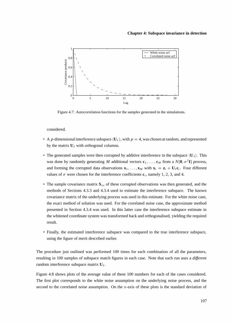
Chapter 4: Subspace invariance in detection
0 5 10 15 20 25 300
0.2
0.4
0.6
0.8
1
Lag
Cov
aria
nce
prod
ucts
White noise acf Correlated noise acf
Figure 4.7: Autocorrelation functions for the samples generated in the simulations.
considered.
• A p-dimensional interference subspace 〈U I 〉, with p = 4, was chosen at random, and represented
by the matrix UI with orthogonal columns.
• The generated samples were then corrupted by additive interference in the subspace 〈U I 〉. This
was done by randomly generating M additional vectors c1, . . . , cM from a N [0, σ 2I] process,
and forming the corrupted data observations x1, . . . , xM with xi = zi + UI ci . Four different
values of σ were chosen for the interference coefficients ci , namely 1, 2, 3, and 4.
• The sample covariance matrix Sx x of these corrupted observations was then generated, and the
methods of Sections 4.3.3 and 4.3.4 used to estimate the interference subspace. The known
covariance matrix of the underlying process was used in this estimate. For the white noise case,
the exact method of solution was used. For the correlated noise case, the approximate method
presented in Section 4.3.4 was used. In this latter case the interference subspace estimate in
the whitened coordinate system was transformed back and orthogonalised, yielding the required
result.
• Finally, the estimated interference subspace was compared to the true interference subspace,
using the figure of merit described earlier.
The procedure just outlined was performed 100 times for each combination of all the parameters,
resulting in 100 samples of subspace match figures in each case. Note that each run uses a different
random interference subspace matrix U I .
Figure 4.8 shows plots of the average value of these 100 numbers for each of the cases considered.
The first plot corresponds to the white noise assumption on the underlying noise process, and the
second to the correlated noise assumption. On the x-axis of these plots is the standard deviation of
107
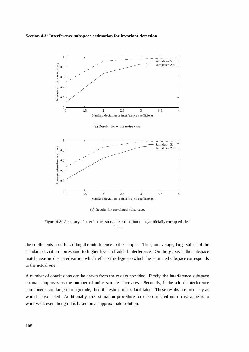
Section 4.3: Interference subspace estimation for invariant detection
1 1.5 2 2.5 3 3.5 40
0.2
0.4
0.6
0.8
1
Standard deviation of interference coefficients
Ave
rage
est
imat
ion
accu
racy
Samples = 50 Samples = 200
(a) Results for white noise case.
1 1.5 2 2.5 3 3.5 40
0.2
0.4
0.6
0.8
1
Standard deviation of interference coefficients
Ave
rage
est
imat
ion
accu
racy
Samples = 50 Samples = 200
(b) Results for correlated noise case.
Figure 4.8: Accuracy of interference subspace estimation using artificially corrupted idealdata.
the coefficients used for adding the interference to the samples. Thus, on average, large values of the
standard deviation correspond to higher levels of added interference. On the y-axis is the subspace
match measure discussed earlier, which reflects the degree to which the estimated subspace corresponds
to the actual one.
A number of conclusions can be drawn from the results provided. Firstly, the interference subspace
estimate improves as the number of noise samples increases. Secondly, if the added interference
components are large in magnitude, then the estimation is facilitated. These results are precisely as
would be expected. Additionally, the estimation procedure for the correlated noise case appears to
work well, even though it is based on an approximate solution.
108
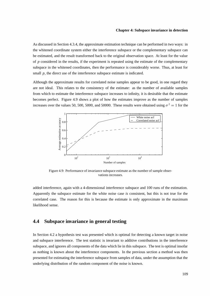
Chapter 4: Subspace invariance in detection
As discussed in Section 4.3.4, the approximate estimation technique can be performed in two ways: in
the whitened coordinate system either the interference subspace or the complementary subspace can
be estimated, and the result transformed back to the original observation space. At least for the value
of p considered in the results, if the experiment is repeated using the estimate of the complementary
subspace in the whitened coordinates, then the performance is considerably worse. Thus, at least for
small p, the direct use of the interference subspace estimate is indicated.
Although the approximate results for correlated noise samples appear to be good, in one regard they
are not ideal. This relates to the consistency of the estimate: as the number of available samples
from which to estimate the interference subspace increases to infinity, it is desirable that the estimate
becomes perfect. Figure 4.9 shows a plot of how the estimates improve as the number of samples
increases over the values 50, 500, 5000, and 50000. These results were obtained using σ 2 = 1 for the
102
103
104
0
0.2
0.4
0.6
0.8
1
Number of samples
Ave
rage
est
imat
ion
accu
racy
White noise acf Correlated noise acf
Figure 4.9: Performance of invariance subspace estimate as the number of sample obser-vations increases.
added interference, again with a 4-dimensional interference subspace and 100 runs of the estimation.
Apparently the subspace estimate for the white noise case is consistent, but this is not true for the
correlated case. The reason for this is because the estimate is only approximate in the maximum
likelihood sense.
4.4 Subspace invariance in general testing
In Section 4.2 a hypothesis test was presented which is optimal for detecting a known target in noise
and subspace interference. The test statistic is invariant to additive contributions in the interference
subspace, and ignores all components of the data which lie in this subspace. The test is optimal insofar
as nothing is known about the interference components. In the previous section a method was then
presented for estimating the interference subspace from samples of data, under the assumption that the
underlying distribution of the random component of the noise is known.
109
Section 4.4: Subspace invariance in general testing
In this section the use of subspace invariant tests is presented for purposes other than detection in
interference. In short, it is argued that such tests may be used in any circumstances where the inclusion of
an invariance subspace either significantly improves the modelling accuracy, or substantially simplifies
the resulting test. In such cases subspace invariance may not seem to be the most natural restriction, and
the resulting tests have no reasonable claim to optimality. However, the formulation may nevertheless
be desirable for other reasons:
• The invariance condition may result in test statistics which are easier to calculate than when the
condition is dropped. Under these circumstances it may be reasonable to find the most powerful
test which has a desirable implementation.
• The data contained in some linear subspace may be in conflict with a convenient assumed
distribution in the observation space. In this instance it may be simpler to just ignore the subspace
where the mismatch is occurring, by requiring invariance to the subspace. The modelling and
testing is then restricted to the conveniently-modelled complementary subspace.
In most cases both of these reasons usually play a role in the decision to use an invariant test.
Figure 4.10 shows two hypothetical scenarios where the use of an invariance subspace may simplify
detection. In both cases a noise probability density is demonstrated which is normally distributed in one
dimension, but where the normal assumption is completely inappropriate in the orthogonal direction.
Rather than attempting to characterise the densities accurately, it may be appropriate to simply ignore
that component of each observation which does not fit the model. This can be achieved by performing
the entire detection procedure on the data value corresponding to the x1-direction, which has a normal
distribution.
More generally, it can happen that the data contained in a p-dimensional subspace do not conform to
an assumption which would otherwise be convenient in the entire N -dimensional space. Under the
MVN assumption, for example, this could happen when the data contained in the subspace 〈U I 〉 are
either not normal, or when the disjoint subspaces 〈UH 〉 and 〈UI 〉 are not jointly normal. It may then
be simpler to just ignore the components of the data in 〈U I 〉, which would otherwise complicate the
statistical description. As long as the target to be detected does not have a considerable component
in the invariance subspace, the performance loss may not be too great. What is gained, however, is
detection performance which is more predictable than if the modelling mismatch were simply ignored.
The notion of ignoring subspaces which do not conform to simple modelling has even more value when
tight constraints are included in the allowable models. Often even the assumption of normality is not
sufficient to simplify the parametric models to the point where they are useful or convenient in practice
— further constraints may be required to yield an accurate parametric distribution which is effective
for the detection. Under a normal assumption, for example, these constraints are brought about by
incorporating dependencies into the mean and covariance parameters of the MVN distribution. The
110
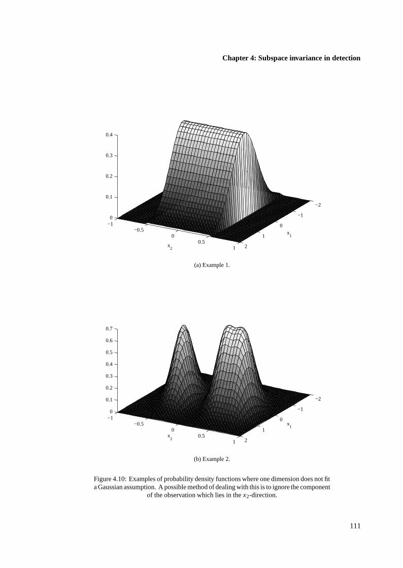
Chapter 4: Subspace invariance in detection
−2
−1
0
1
2
−1−0.5
00.5
1
0
0.1
0.2
0.3
0.4
x1
x2
(a) Example 1.
−2
−1
0
1
2
−1−0.5
00.5
1
0
0.1
0.2
0.3
0.4
0.5
0.6
0.7
x1
x2
(b) Example 2.
Figure 4.10: Examples of probability density functions where one dimension does not fita Gaussian assumption. A possible method of dealing with this is to ignore the component
of the observation which lies in the x2-direction.
111

Section 4.5: Invariance subspace estimation for model mismatch
constraints can enhance the convenience and tractability of the model, but also increase the possibility
of mismatch between the assumed and the actual distributions. If the mismatches tend to be restricted
to a linear subspace of the observation space, however, the use of subspace invariance can simplify the
detection problem and improve performance.
In the previous section it was demonstrated that the invariant test in Equation 4.30 is optimal for the
detection problem where interference in a known subspace is present in the observation. This is no
longer true when invariance is applied in the context suggested here: because the invariance condition
cannot be claimed to be natural for the problem, the requirement that a test be invariant involves a
restriction which cannot by justified entirely on decision-theoretic grounds. Rather, the justification
lies in the convenience of the representation, which in practice may ultimately result in better modelling
accuracy. The test is still uniformly most powerful within the class of invariant tests, but this criterion
is no longer of any use as an optimality property.
By incorporating invariance into the hypothesis test, the invariance dimensions are entirely ignored in
the calculation of the statistic. If the target to be detected happens to lie in the invariance subspace,
this will lead to a complete failure of the detection procedure. The only recourse then is to improve
the accuracy of the statistical model used to characterise the noise. If part of the target lies in the
ignored subspace, there will be a loss in detectability brought about by the effective reduction in the
target energy. This will lead to a degradation in detection performance. However, if the invariance
subspace significantly improves the modelling accuracy, an increase in the overall performance may
still be effected.
Improved modelling accuracy will result in a test which exhibits performance closer to the design
performance. Thus detection and false alarm probabilities will be closer to the values expected from
the design stage. This is important in practical detectors. Also, it is easier to have confidence in a
system which performs in accordance with predictions, since it reflects a deeper understanding of the
processes being modelled.
4.5 Invariance subspace estimation for model mismatch
Section 4.3 discussed the problem of estimating the interference subspace from noise samples con-
taining interference. The assumption was made that the distribution of the random component of the
observations is multivariate normal, with known mean and covariance. It was demonstrated that inter-
ference causes an increase in the variance of the data in the corresponding dimensions. This increased
variance can be identified, and estimated interference subspaces assigned accordingly.
However, as suggested in the previous section, the notion of subspace invariance in testing also has
application in reducing the mismatch between assumed models and actual data realisations. Identifying
112
Chapter 4: Subspace invariance in detection
candidate invariance subspaces for this problem is different from that of identification of interference
subspaces. The primary reason for this difference arises in that a mismatched model can exhibit
variances in certain directions which are greater than or smaller than the variances predicted by
the model. This cannot occur under the subspace interference interpretation, where only increased
variances may be observed.
The likelihood criterion used for interference subspace estimation therefore cannot always be applied
sensibly to the problem of model mismatch. A modified criterion is required which penalises both
mismatch in terms of variances which are larger than those predicted by the model, as well as those
which are smaller.
The solutions to this identification problem depend strongly on the criterion used to assess mismatch.
Also, as with the subspace interference problem, most formulations are not tractable and are therefore
not useful in practice. One criterion which is reasonable and useful is based on the Frobenius norm,
which can be used to measure the distance between covariances matrices of the model and the observa-
tions. In this section a method of invariance subspace estimation is presented, based on this criterion.
An example of invariance subspace estimation applied to a real-data problem is then presented in
Section 4.5.2.
4.5.1 Formulation of invariance subspace estimate
Suppose that the assumed model covariance is C, and that the sample covariance of the observations
is Sx x . As before, this sample covariance is calculated under the assumption that the noise mean
under H0 is known, and equal to m0. C is again assumed known, and may be chosen to have a form
that is convenient from a computational perspective. The approach taken in the invariance subspace
identification problem is to find a subspace 〈U I 〉 where these two covariance matrices are maximally
different. If such a subspace is ignored in subsequent estimation and detection, a reduction in model
mismatch will be achieved.
Since the invariance subspace is spanned by U I , the model covariance in 〈UI 〉 is UTI CUI . Similarly,
the sample covariance in this subspace is UTI Sx xUI . Now, the Frobenius norm measures the mismatch
between two matrices F and G as the sum of the squared differences between the corresponding
elements. Thus, if F = ( f i j ) and G = (gi j ), then the distance between the matrices in the specified
metric is
dF (F, G) =p∑
i=1
p∑
j=1
( fi j − gi j )2
= tr(F − G)T (F − G), (4.73)
where the dimension of the matrices is assumed to be p× p. The distance between the model covariance
113
Section 4.5: Invariance subspace estimation for model mismatch
and the actual covariance is therefore given by
dF(UTI Sx xUI , UT
I CUI ) = tr{UT
I (Sx x − C)UI UTI (Sx x − C)UI
}
= tr{UT
I AUI UTI AUI
}, (4.74)
where use has been made of the symmetry of C and Sx x , and A = Sx x − C for convenience.
Under this proposed criterion, a good invariance subspace will be associated with a choice of U I where
the distance in Equation 4.74 is large. In the remainder of this section it is shown that the distance
is maximised when the columns of U I are chosen to be those eigenvectors of A corresponding to the
p eigenvalues with largest absolute magnitude. The distance measure chosen depends only on the
subspace spanned by the matrix U I . That is, if UI is replaced by any matrix UI R with R unitary, the
distance remains unchanged:
tr{(UI R)T A(UI R)(UI R)T A(UI R)
}= tr
{RT UT
I AUI UTI AUI R
}= tr
{UT
I AUI UTI AUI
}. (4.75)
This is important since it again means that it is only the subspace 〈U I 〉 that is important in the max-
imisation, not the specific details of U I .
As before, we assume that UH is a matrix with orthogonal columns such that UTH UI = I. The distance
dF can then be written as
dF = tr{UT
I A(I − UH UTH)AUI
}
= tr{UT
I AAUI
}− tr
{UT
I AUH UTH AUI
}. (4.76)
Letting UH = (h1 · · · hn−p) and UI = (i1 · · · ip), the second term in this expression is
tr{UT
I AUH UTH AUI
}= iT
1 A
n−p∑
j=1
h j hTj
Ai1 + · · · + iT
p A
n−p∑
j=1
h j hTj
Aip
=p∑
k=1
n−p∑
j=1
iTk Ah jhT
j Aik =p∑
k=1
n−p∑
j=1
(iTk Ah j)
2, (4.77)
where the final result holds on account of the symmetry of A. This result demonstrates that the second
term in Equation 4.76 is a nonnegative quantity, irrespective of the choice of U I and UH .
Using the previous observation, an upper bound on the value of dF under the required orthogonality
constraints can be found. Specifically, since the second term in Equation 4.76 is nonnegative, the
quantity dF must always be smaller than or equal to the maximum attainable value of tr{UT
I AAUI
}.
Under the constraint that UTI UI = I, it is possible to calculate this maximum value. Forming the
114
Chapter 4: Subspace invariance in detection
Lagrangian� = tr
{UT
I AAUI
}+
p∑
j=1
p∑
k≥ j
λ j kg j k(i1, . . . , ip) (4.78)
with the final term representing the orthogonality constraint, it is easy to show that
d�
dUI= 2AAUI + 2UI 0. (4.79)
To achieve a maximum, this derivative must be zero when evaluated at U I = UI :
2AAUI + 2UI 0 = 0. (4.80)
Premultiplying by UTI ,
20 = −2UTI AAUI , (4.81)
so a necessary condition on UI is that
UI UTI AAUI = AAUI . (4.82)
This is exactly the problem discussed in Section 4.3.3. There it was shown that to maximise the
required trace, one solution is to choose as the columns of UI the eigenvectors corresponding to the
p largest eigenvalues. The maximum value attained for tr{UT
I AAUI
}is in that case the sum of the
corresponding eigenvalues. Now, since AA is the Grammian of A, it is positive semidefinite. Thus
the eigenvalues involved in this sum are all nonnegative. Given A, it is easy to calculate the maximum
possible value that dF may have: it is simply the sum of the p largest eigenvalues of AA.
It is now shown that there exists a choice of UI and UH for which the distance dF attains the maximum
possible value derived in the previous paragraph. Clearly, then, this provides the required solution to
the maximisation problem. In particular, we take UI to be comprised of eigenvectors corresponding
to the p eigenvalues of A with maximum absolute magnitude. The matrix UH is taken to be the
n − p remaining eigenvectors, which correspond to eigenvalues with smallest magnitude. Since A is
symmetric, all these eigenvalues are real, although some may be negative. With the preceeding choice
of UI and UH , it is clearly true that UTI AUI = 3I , UT
H AUH = 3H , and UTI AUH = 0, which are
basic properties of eigenvectors. In these relationships 3 I is a diagonal matrix containing the p largest
absolute eigenvalues of A, and 3H is a diagonal matrix containing the smallest.
Returning to the expression in Equation 4.76, under the conditions described, the second term is
identically zero since UTI AUH = 0. The achieved distance between the matrices is therefore
dF = tr{UT
I AAUI
}. (4.83)
115
Section 4.5: Invariance subspace estimation for model mismatch
This distance can be written as
dF = tr{(AUI )
T (AUI )}
= tr{(UI 3I )
T (UI 3I )}
= tr(32
I
). (4.84)
This is exactly the sum of the squared eigenvalues of A which have largest magnitude.
Finally, if λ is an eigenvalue of A, then λ2 is an eigenvalue of AA. Thus if {λ1, . . . , λp} is the set of
eigenvalues of A with largest magnitude, then {λ21, . . . , λ
2p} will be the set of largest eigenvalues of
AA. Now, since
tr(32
I
)=
p∑
j=1
λ2j , (4.85)
it is evident that dF meets the upper bound on the distance, since the sum of the squared values of the
eigenvalues of A with maximum absolute value is identical to the sum of the maximum eigenvalues of
AA. Thus UI maximises the distance between the covariance matrices, as required.
The method discussed can be used to find the invariance subspace which maximises the Frobenius
distance between the model and sample covariances within that subspace. It seems, however, that
the same method cannot be used to estimate the complementary subspace U H through an analogous
minimisation of the corresponding distances. For example, if it is required to find a single dimension
h where the mismatch is small, any unit vector h such that hT Ch = hT Sx xh should be appropriate.
Thus h should be chosen to be one of those directions where the variance of C and Sx x are equal. In
general this will not occur for h an eigenvector of Sx x − C.
4.5.2 Example of invariance subspace estimation
The invariance subspace estimate presented in the previous section can be used whenever the underlying
data covariance matrix is assumed known. The invariance subspace then serves to reduce the degree
of mismatch between the model and a set of data samples, by identifying those dimensions where the
model and sample covariances differ most.
In most cases the underlying covariance matrix is not known. However, for any covariance assumption,
the method presented will tend to produce an invariance subspace which will enhance the degree of
match between the data and the model. For purposes of demonstrating the concept, therefore, the
underlying covariance assumption is not critical. In this section a fairly arbitrary covariance assumption
is made, and it is demonstrated how a subspace invariance restriction can result in a detector which
exhibits both better and more predictable performance than a noninvariant detector.
The test data used for the demonstration is shown in Figure 4.11. It is a portion of a x-ray image of a
scale model of a mill, of a type used in the mining industry. Also shown in the figure is a horizontal cut
along the first line of the image, clearly demonstrating a nonstationary trend in the data. The problem
116

Chapter 4: Subspace invariance in detection
(a) Complete image.
50 100 150 200 250 300 350−30
−20
−10
0
10
20
Horizontal position
Inte
nsity
(b) Horizontal cut through first line.
Figure 4.11: Test image used in analysis.
discussed here is that of detecting a known target in a horizontal 32 element sample of noise. For
the demonstration, noise samples are obtained by simply extracting data from various locations in the
image. Note that this procedure is in no direct way related to either the detection of a 2-D target in
the image, or the problem of detecting a target with unknown location. The image is simply used to
provide 1-D noise samples which are related to one another in a realistic but unknown manner.
It is assumed that the target to be detected is a transient one-dimensional Gaussian signal with a
standard deviation of 3 and an energy of 50 × 50 = 2500. The assumption is also made that the
nominal distribution of the noise is stationary, with an autocorrelation function
r( j) = 15(0.8) j . (4.86)
The image was made to have a mean of zero prior to the processing, so the noise in the model is
assumed zero mean.
If a detector is developed using this arbitrary assumed model, it will clearly be inaccurate. Nevertheless,
such a detector was designed, and applied to a set of overlapping noise samples extracted from the 20th
to 30th lines in the test image. This led to a set of sample test statistic values under the H0 assumption.
117

Section 4.5: Invariance subspace estimation for model mismatch
The solid plot in Figure 4.12(a) shows the values of each of these samples for noise data extracted from
the 20th line. Also shown in Figure 4.12(a), and represented by the dashed plot, is the value that the
50 100 150 200 250 300 350−40
−20
0
20
40
60
80
Horizontal position
Tes
t sta
tistic
val
ue
Target absent Target present
(a) No invariance subspace.
50 100 150 200 250 300 350−20
−10
0
10
20
30
40
Horizontal position
Tes
t sta
tistic
val
ue
Target absent Target present
(b) Invariance subspace of dimension 3.
Figure 4.12: Example of test statistic applied to 20th line of test image.
test statistic would take on in the event that there was a target present in each extracted sample of data.
If the two sets of test statistic values were well-separated, then comparing the statistic to a threshold
would provide a good test. However, in this case the distributions of the values overlap considerably,
on account of the inaccuracy of the model used to derive the detector.
Figure 4.12(b) shows a similar result, this time using a detector designed with a 3-dimensional in-
variance subspace. This invariance subspace was estimated using noise samples obtained from the
first 10 rows of the test data. In particular, for each of the 10 lines, a noise sample of length 32
was extracted from horizontal positions separated by a distance of 8 pixels, and a sample covariance
matrix calculated. Using this sample covariance and the assumed noise covariance, a 3-dimensional
118
Chapter 4: Subspace invariance in detection
invariance subspace was obtained using the methods of the previous section. This invariance subspace
was then used in conjunction with the assumed covariance to develop an invariant detection statistic,
which was tested in the same manner described for the noninvariant detector. The invariant detector
quite successfully ignores those components of the data which represent the most significant model
mismatch. That is, the sets of values taken on under target-absent and target-present conditions are
well separated and compact, and a threshold on the invariant test statistic will produce an effective test.
The invariance subspace has reduced the absolute separation between the values taken on between
the two hypotheses. For the noninvariant detector this separation is approximately 40, while for the
invariant detector it is about 20. However, on account of the better model match, the observed variance
of the test statistic is considerably smaller for the invariant detector. If the separation in each case is
considered as a fraction of the standard deviation of the noise in the statistic, then it is apparent that
this normalised separation is greater for the invariant detector. Figure 4.13 shows this normalisation as
a function of the invariance subspace dimension. As the invariance subspace increases, the normalised
separation increases initially and then tails off as the dimension of the invariance subspace increases
further. The initial rise is caused by the subspace invariance reducing the standard deviation of the
noise in the test statistic; the subsequent dropoff is a result of progressively more of the target being
nulled by the invariant detector.
Also shown in Figure 4.13 is the predicted and the observed standard deviations of the test statistic when
applied to the noise data. The predicted value is obtained using the assumed model distribution, from
which the original detectors were derived. It can be seen that as the dimension of the invariance subspace
increases, the mismatch between the predicted standard deviation and the observed standard deviation
decreases. This quite simply occurs because the invariant model is more accurate for representing the
data than the noninvariant model.
119
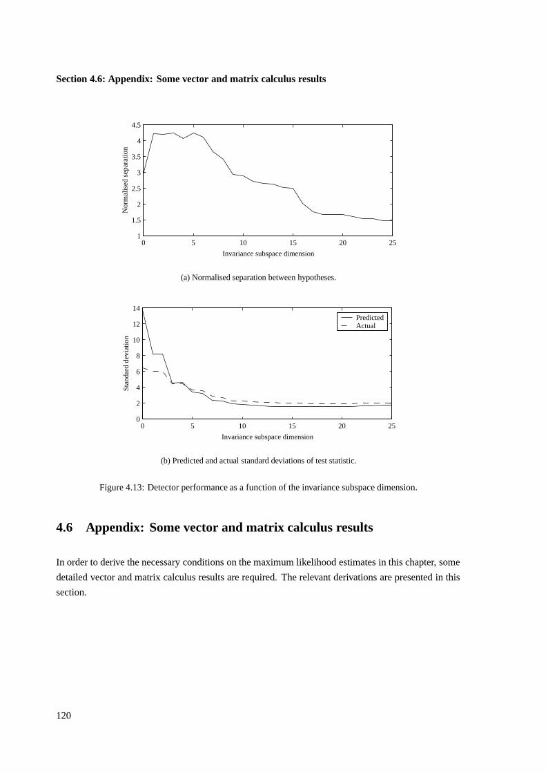
Section 4.6: Appendix: Some vector and matrix calculus results
0 5 10 15 20 251
1.5
2
2.5
3
3.5
4
4.5
Invariance subspace dimension
Nor
mal
ised
sep
arat
ion
(a) Normalised separation between hypotheses.
0 5 10 15 20 250
2
4
6
8
10
12
14
Invariance subspace dimension
Stan
dard
dev
iatio
n
PredictedActual
(b) Predicted and actual standard deviations of test statistic.
Figure 4.13: Detector performance as a function of the invariance subspace dimension.
4.6 Appendix: Some vector and matrix calculus results
In order to derive the necessary conditions on the maximum likelihood estimates in this chapter, some
detailed vector and matrix calculus results are required. The relevant derivations are presented in this
section.
120
Chapter 4: Subspace invariance in detection
4.6.1 dy/dθ of y = y(x(θ)):
dy
dθ=
ddθ1
y(x1(θ1, . . . , θm), . . . , xn(θ1, . . . , θm))
...d
dθmy(x1(θ1, . . . , θm), . . . , xn(θ1, . . . , θm))
=
dydx1
dx1dθ1
+ · · · + dydxn
dxndθ1
...dydx1
dx1dθm
+ · · · + dydxn
dxndθm
=
dx1dθ1
. . . dxndθ1
.... . .
...dx1dθm
. . . dxndθm
dydx1...
dydxn
= dxdθ
dy
dx. (4.87)
4.6.2 dy/dθ of y = vT (θ)w(θ):
Rewriting as y = v1(θ)w1(θ) + · · · + vn(θ)wn(θ), the derivative with respect to θ is
dy
dθ=
dydθ1...
dydθm
=
v1dw1dθ1
+ w1dv1dθ1
+ · · · + vndwndθ1
+ wndvndθ1
...
v1dw1dθm
+ w1dv1dθm
+ · · · + vndwndθm
+ wndvndθm
= dwdθ
v + dvdθ
w. (4.88)
4.6.3 dv/dθ of v = A(θ)u(θ):
If A is the matrix
A =
a11 · · · a1n...
. . ....
an1 · · · ann
=
aT1...
aTn
,
then the i th component of v is given by
vi(θ) = aTi (θ)ui(θ).
121
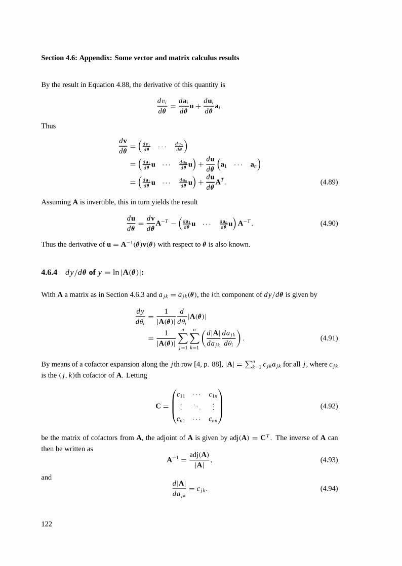
Section 4.6: Appendix: Some vector and matrix calculus results
By the result in Equation 4.88, the derivative of this quantity is
dvi
dθ= dai
dθu + dui
dθai .
Thus
dvdθ
=(
dv1dθ
· · · dvndθ
)
=(
da1dθ
u · · · dandθ
u)
+ dudθ
(a1 · · · an
)
=(
da1dθ
u · · · dandθ
u)
+ dudθ
AT . (4.89)
Assuming A is invertible, this in turn yields the result
dudθ
= dvdθ
A−T −(
da1dθ
u · · · dandθ
u)
A−T . (4.90)
Thus the derivative of u = A−1(θ)v(θ) with respect to θ is also known.
4.6.4 dy/dθ of y = ln |A(θ)|:
With A a matrix as in Section 4.6.3 and a j k = a j k(θ), the i th component of dy/dθ is given by
dy
dθi= 1
|A(θ)|d
dθi|A(θ)|
= 1
|A(θ)|
n∑
j=1
n∑
k=1
(d|A|da j k
da j k
dθi
). (4.91)
By means of a cofactor expansion along the j th row [4, p. 88], |A| =∑n
k=1 c j ka j k for all j , where c j k
is the ( j, k)th cofactor of A. Letting
C =
c11 · · · c1n...
. . ....
cn1 · · · cnn
(4.92)
be the matrix of cofactors from A, the adjoint of A is given by adj(A) = CT . The inverse of A can
then be written as
A−1 = adj(A)
|A| , (4.93)
andd|A|da j k
= c j k . (4.94)
122
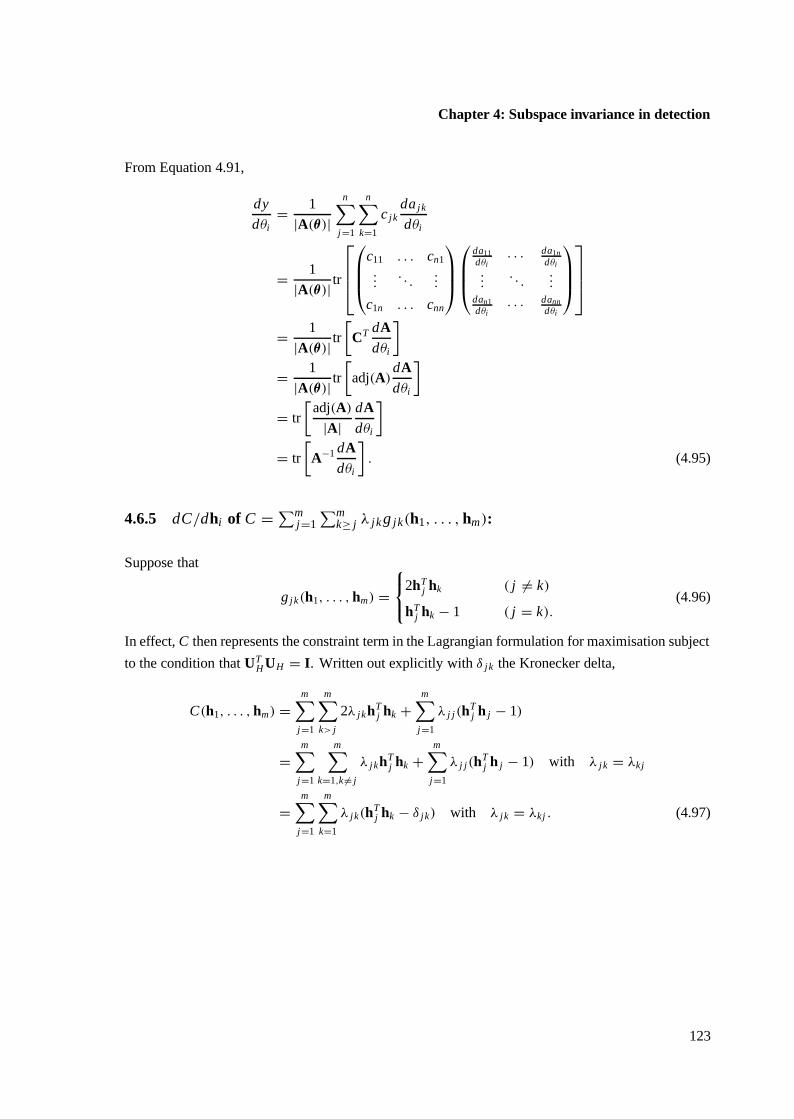
Chapter 4: Subspace invariance in detection
From Equation 4.91,
dy
dθi= 1
|A(θ)|
n∑
j=1
n∑
k=1
c j kda j k
dθi
= 1
|A(θ)| tr
c11 . . . cn1...
. . ....
c1n . . . cnn
da11dθi
· · · da1ndθi
.... . .
...dan1dθi
· · · danndθi
= 1
|A(θ)| tr[
CT dAdθi
]
= 1
|A(θ)| tr[
adj(A)dAdθi
]
= tr
[adj(A)
|A|dAdθi
]
= tr
[A−1 dA
dθi
]. (4.95)
4.6.5 dC/dhi of C =∑m
j=1∑m
k≥ j λ jk g jk(h1, . . . , hm):
Suppose that
g j k(h1, . . . , hm) =
2hTj hk ( j 6= k)
hTj hk − 1 ( j = k).
(4.96)
In effect, C then represents the constraint term in the Lagrangian formulation for maximisation subject
to the condition that UTH UH = I. Written out explicitly with δ j k the Kronecker delta,
C(h1, . . . , hm) =m∑
j=1
m∑
k> j
2λ j khTj hk +
m∑
j=1
λ j j(hTj h j − 1)
=m∑
j=1
m∑
k=1,k 6= j
λ j khTj hk +
m∑
j=1
λ j j(hTj h j − 1) with λ j k = λkj
=m∑
j=1
m∑
k=1
λ j k(hTj hk − δ j k) with λ j k = λkj . (4.97)
123

Section 4.6: Appendix: Some vector and matrix calculus results
The required derivatives are now given by
dC
dhi= d
dhi
m∑
k=1
λik(hTi hk − δik) +
m∑
j=1
λ j i(hTj hi − δ j i) − λii(hT
i hi − δii )
= d
dhi
m∑
k=1,k 6=i
λikhTi hk +
m∑
j=1, j 6=i
λ j ihTj hi + λii (hT
i hi − 1)
=m∑
k=1,k 6=i
λikhk +m∑
j=1, j 6=i
λ j ih j + 2λii hi
=m∑
k=1
λikhk +m∑
j=1
λ j ih j , (4.98)
which, since λ j k = λkj , is equal to
dC
dhi=
m∑
k=1
λikhk +m∑
j=1
λi j h j
= 2m∑
k=1
λikhk
= 2(
h1 · · · hm
)
λi1...
λim
= 2UHλi . (4.99)
Thus letting 0 be the symmetric matrix 0 = (λ1 · · · λm) with λTi = (λi1 · · · λim),
dC
dUH= 2UH (λi1 · · · λim) = 2UH0. (4.100)
4.6.6 dy/dUH of y = ln |UTH CUH |:
Suppose UH = (h1 · · · hm) and
h j =
h j1...
h jn
. (4.101)
Letting X = UTH CUH , the result in Section 4.6.4 shows that
dy
dh j k= tr
[X−1 dX
dh j k
]. (4.102)
124

Chapter 4: Subspace invariance in detection
Initially, it is therefore required to calculate the derivative with respect to h j k of
X =
hT1 Ch1 · · · hT
1 Chm...
. . ....
hTmCh1 · · · hT
mChm
. (4.103)
Letting CT = (c1 · · · cm), there are four cases of interest which occur in the derivative of the elements
hTr Chs of X:
• j = r, j 6= s : Letting ys = Chs , ddh jk
hTr Chs = d
dh jkhT
j Chs . Therefore
d
dh j khT
r Chs = d
dh j k
(h j1 · · · h jn
)
ys1...
hsn
= ynk = cT
k hs. (4.104)
• j = s, j 6= r : ddh jk
hTr Chs = d
dh jkhT
r Ch j = cTk hr .
• j = r, j = s : ddh jk
hTr Chs = d
dh jkhT
j Ch j . However ddh j
hTj Ch j = 2Chi = 2yi , so
d
dh j khT
r Chs = 2y j k = 2cTk h j . (4.105)
• j 6= r, j 6= s : ddh jk
hTr Chs = 0.
Using these results,
d
dh j kUT
H CUH =
0 · · · cTk h1 · · · 0
......
...
cTk h1 · · · 2cT
k h j · · · cTk hm
......
...
0 · · · cTk hm · · · 0
,
where only the j th row and column have nonzero elements. This matrix can be written as
d
dh j kUT
H CUH =
0 · · · 0 · · · 0...
......
cTk h1 · · · cT
k h j · · · cTk hm
......
...
0 · · · 0 · · · 0
+
0 · · · cTk h1 · · · 0
......
...
0 · · · cTk h j · · · 0
......
...
0 · · · cTk hm · · · 0
= e j cTk UH + UT
H ck eTj , (4.106)
125
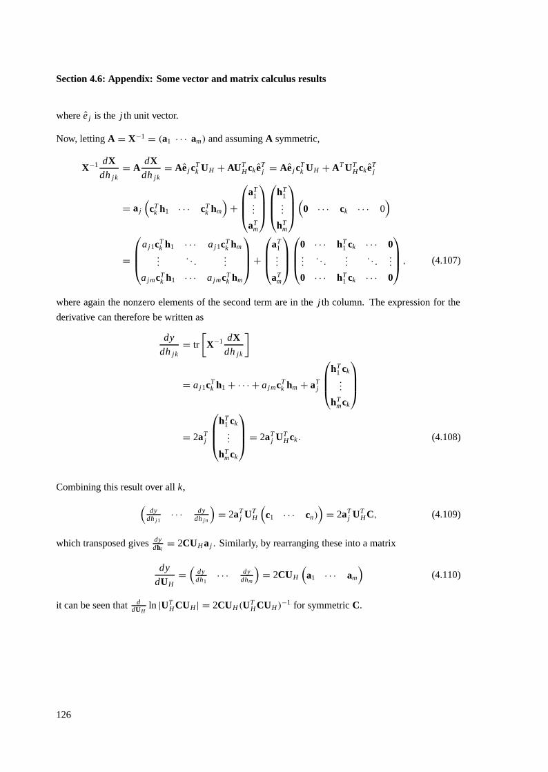
Section 4.6: Appendix: Some vector and matrix calculus results
where e j is the j th unit vector.
Now, letting A = X−1 = (a1 · · · am) and assuming A symmetric,
X−1 dXdh j k
= AdX
dh j k= Ae j cT
k UH + AUTH ck eT
j = Ae j cTk UH + AT UT
H ck eTj
= a j
(cT
k h1 · · · cTk hm
)+
aT1...
aTm
hT1...
hTm
(
0 · · · ck · · · 0)
=
a j1cTk h1 · · · a j1cT
k hm...
. . ....
a jmcTk h1 · · · a jmcT
k hm
+
aT1...
aTm
0 · · · hT1 ck · · · 0
.... . .
.... . .
...
0 · · · hT1 ck · · · 0
, (4.107)
where again the nonzero elements of the second term are in the j th column. The expression for the
derivative can therefore be written as
dy
dh j k= tr
[X−1 dX
dh j k
]
= a j1cTk h1 + · · · + a jmcT
k hm + aTj
hT1 ck...
hTmck
= 2aTj
hT1 ck...
hTmck
= 2aT
j UTH ck . (4.108)
Combining this result over all k,
(dy
dh j1· · · dy
dh jn
)= 2aT
j UTH
(c1 · · · cn)
)= 2aT
j UTH C, (4.109)
which transposed gives dydhi
= 2CUH a j . Similarly, by rearranging these into a matrix
dy
dUH=(
dydh1
· · · dydhm
)= 2CUH
(a1 · · · am
)(4.110)
it can be seen that ddUH
ln |UTH CUH | = 2CUH(UT
H CUH)−1 for symmetric C.
126
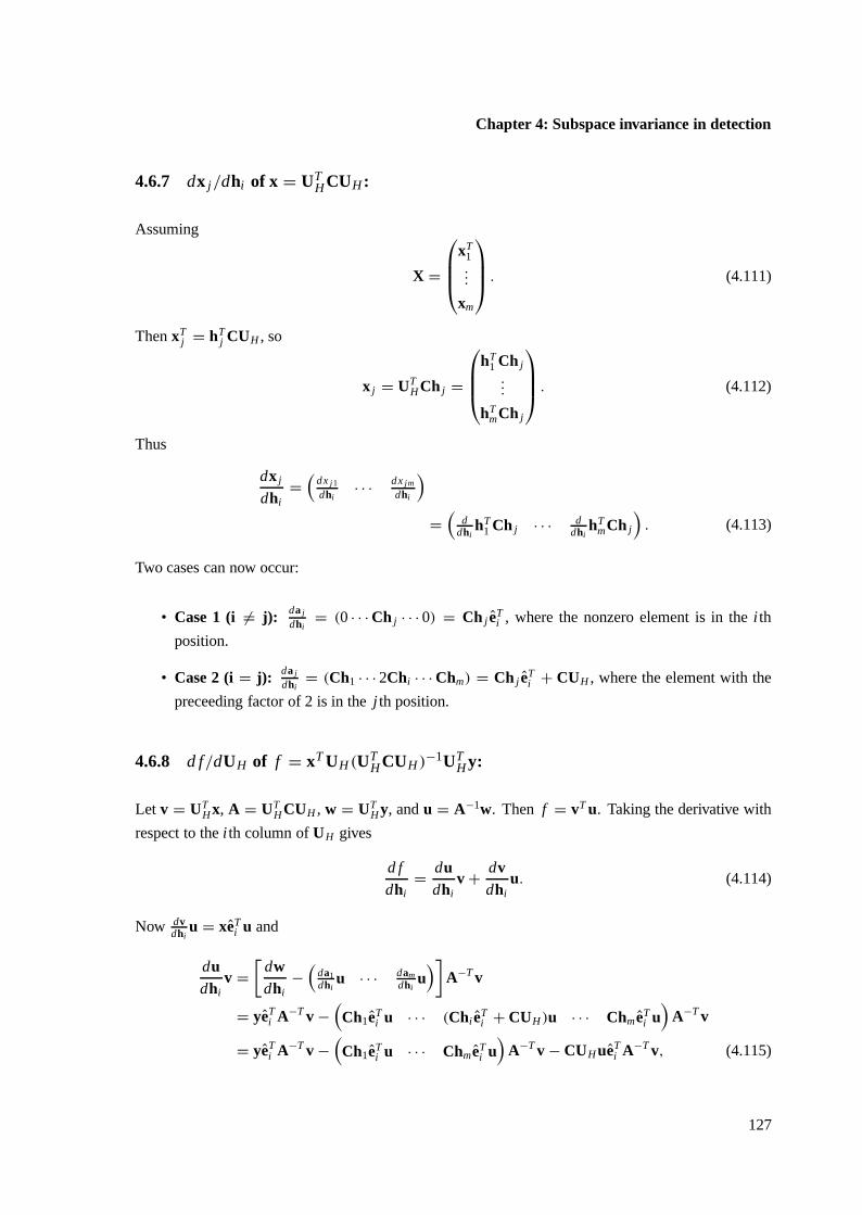
Chapter 4: Subspace invariance in detection
4.6.7 dx j/dhi of x = UTH CUH :
Assuming
X =
xT1...
xm
. (4.111)
Then xTj = hT
j CUH , so
x j = UTH Ch j =
hT1 Ch j
...
hTmCh j
. (4.112)
Thus
dx j
dhi=(
dx j1
dhi· · · dx jm
dhi
)
=(
ddhi
hT1 Ch j · · · d
dhihT
mCh j
). (4.113)
Two cases can now occur:
• Case 1 (i 6= j): da j
dhi= (0 · · · Ch j · · · 0) = Ch j eT
i , where the nonzero element is in the i th
position.
• Case 2 (i = j): da j
dhi= (Ch1 · · · 2Chi · · · Chm) = Ch j eT
i + CUH , where the element with the
preceeding factor of 2 is in the j th position.
4.6.8 d f/dUH of f = xT UH (UTH CUH )−1UT
H y:
Let v = UTH x, A = UT
H CUH , w = UTH y, and u = A−1w. Then f = vT u. Taking the derivative with
respect to the i th column of UH gives
d f
dhi= du
dhiv + dv
dhiu. (4.114)
Now dvdhi
u = xeTi u and
dudhi
v =[
dwdhi
−(
da1dhi
u · · · damdhi
u)]
A−T v
= yeTi A−T v −
(Ch1eT
i u · · · (Chi eTi + CUH)u · · · Chm eT
i u)
A−T v
= yeTi A−T v −
(Ch1eT
i u · · · Chm eTi u)
A−T v − CUH ueTi A−T v, (4.115)
127
so
d f
dhi= xeT
i u + yeTi A−T v − CUH ueT
i A−T v −(
Ch1eTi u · · · Chm eT
i u)
A−T v. (4.116)
But
(Ch1eT
i u · · · Chm eTi u)
A−T v = (eTi u)
(Ch1 · · · Chm
)A−T v
= (eTi u)CUHA−T v = CUH A−T veT
i u, (4.117)
which, letting z = A−T v, yields for the derivative
d f
dhi= (x − CUH A−T v)eT
i u + (y − CUHu)eTi A−T v
= (x − CUH A−T v)ui + (y − CUH u)zi . (4.118)
Arranging the individual results for each i into a matrix and substituting the original assignments,
d f
dUH=(
d fdh1
· · · d fdhm
)
= (x − CUH A−T v)uT + (y − CUHu)zT
= xyT UH(UTH CUH)−T − CUH(UT
H CUH)−T UTH xyT UH(UT
H CUH)−T
+ yxT UH(UTH CUH)−1 − CUH(UT
H CUH)−1UTH yxT UH(UT
H CUH)−1
= (I − CUH(UTH CUH)−T UT
H)xyT UH(UTH CUH)−T +
+ (I − CUH(UTH CUH)−1UT
H)yxT UH(UTH CUH)−1. (4.119)
If C is symmetric, this simplifies to
d f
dUH= (I − CUH(UT
H CUH)−1UTH)(xyT + yxT )UH(UT
H CUH)−1, (4.120)
and if additionally y = x, then
d f
dUH= 2(I − CUH(UT
H CUH)−1UTH)xxT UH(UT
HCUH)−1. (4.121)
Note that since y = xT UH(UTH CUH)−1UT
H x is equivalent to y = tr{(UT
H CUH)−1UTH xxT UH
}, this
result can also be written as
d
dUHtr{(UT
H CUH)−1UTH xxT UH
}= 2(I − CUH(UT
H CUH)−1UTH)xxT UH(UT
H CUH)−1. (4.122)
128
Chapter 5
Subspace invariant covariance estimation
In the previous chapter, the uniformly most powerful invariant test was presented for the problem
of detecting a target in MVN noise with known parameters and interference in a known subspace.
Methods were suggested for estimating the interference subspace from actual samples of data, still
under the assumption that the noise mean and covariance parameters are known. The use of invariant
detectors for more general problems was also proposed, where the invariance subspace is used to
partially overcome the effects of model mismatch, specifically in the cases where such mismatch
occurs in a low-dimensional subspace of the observation space.
All the results of Chapter 4 make the assumption that the parameters of the underlying noise process
are known. Samples of data are then used to estimate a suitable invariance subspace. In this chapter the
dual problem is addressed, where the invariance subspace is assumed known but the noise parameters
are unknown and have to be estimated. Again the assumption is made of a nominally MVN distribution
for the noise, at least within the subspace complementary to the invariance subspace.
In general, if not accounted for, the presence of subspace interference or low-rank model mismatch will
have an effect on any noise parameter estimates. Take for example the simple 2-D situation depicted
in Figure 5.1, where the actual noise is zero mean and uncorrelated, and interference is present in the
x2-direction. For purposes of estimation, the assumption is made that the noise mean is identically zero,
and the covariance is some unknown multiple of the identity matrix, say σ 2I. To specify the noise, it
is required to estimate σ 2. Now, if σ 2 is estimated without suitable compensation for the interference,
a reasonable estimator would be the average of the sample variance in the x1 and x2-directions. The
resulting covariance estimate is demonstrated by the dotted contour in Figure 5.1, where it is clear that
the value of σ 2 has been considerably overestimated.
For the case of the data being corrupted by interference in the subspace 〈U I 〉, one remedy is to consider
the interference subspace components unknown and estimate them along with the model parameters.
129
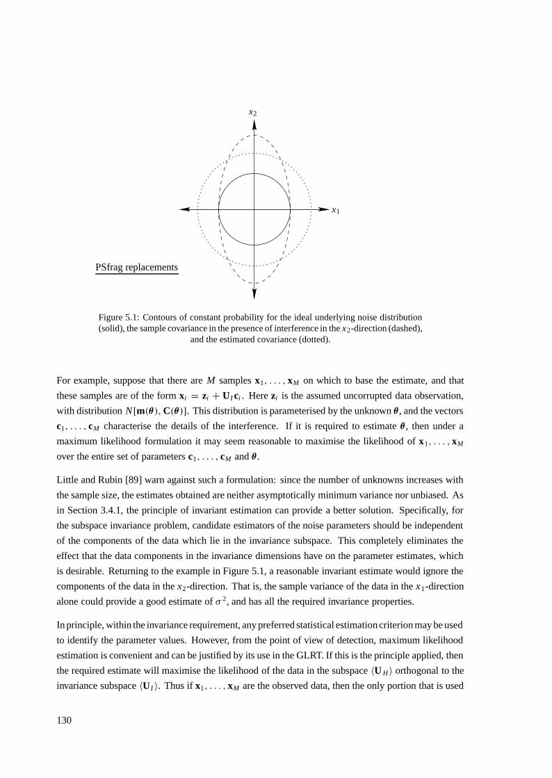
PSfrag replacements
x1
x2
Figure 5.1: Contours of constant probability for the ideal underlying noise distribution(solid), the sample covariance in the presence of interference in the x2-direction (dashed),
and the estimated covariance (dotted).
For example, suppose that there are M samples x1, . . . , xM on which to base the estimate, and that
these samples are of the form xi = zi + UI ci . Here zi is the assumed uncorrupted data observation,
with distribution N [m(θ), C(θ)]. This distribution is parameterised by the unknown θ , and the vectors
c1, . . . , cM characterise the details of the interference. If it is required to estimate θ , then under a
maximum likelihood formulation it may seem reasonable to maximise the likelihood of x1, . . . , xM
over the entire set of parameters c1, . . . , cM and θ .
Little and Rubin [89] warn against such a formulation: since the number of unknowns increases with
the sample size, the estimates obtained are neither asymptotically minimum variance nor unbiased. As
in Section 3.4.1, the principle of invariant estimation can provide a better solution. Specifically, for
the subspace invariance problem, candidate estimators of the noise parameters should be independent
of the components of the data which lie in the invariance subspace. This completely eliminates the
effect that the data components in the invariance dimensions have on the parameter estimates, which
is desirable. Returning to the example in Figure 5.1, a reasonable invariant estimate would ignore the
components of the data in the x2-direction. That is, the sample variance of the data in the x1-direction
alone could provide a good estimate of σ 2, and has all the required invariance properties.
In principle, within the invariance requirement, any preferred statistical estimation criterion may be used
to identify the parameter values. However, from the point of view of detection, maximum likelihood
estimation is convenient and can be justified by its use in the GLRT. If this is the principle applied, then
the required estimate will maximise the likelihood of the data in the subspace 〈U H 〉 orthogonal to the
invariance subspace 〈UI 〉. Thus if x1, . . . , xM are the observed data, then the only portion that is used
130
Chapter 5: Subspace invariant covariance estimation
in the invariant estimation is UTH x1, . . . , UT
H xM , which are the components of the observations which
lie outside of the invariance subspace. The invariant MLE will maximise the likelihood of observing
these portions of the observations with respect to the unknown parameter values.
The presence of constraints on the noise parameters can cause some complications in the context of
invariant estimation. This is because constraints on the assumed MVN model may conceptually be
applied in two ways: either to the distribution of the data in the original observation space, or to the
distribution of the data in the subspace that is considered valid for estimation. By placing the constraint
on the valid components of the data, the invariance subspace is entirely removed from the problem.
The constrained estimate then makes no reference whatsoever to any conditions or constraints in the
original observation space, and the constrained maximisation can be performed directly. For example,
an assumption might be made that the portion of an observation outside of the invariance subspace is
subject to a white noise constraint. This constraint is phrased entirely within the subspace 〈U H 〉, and
no reference is made to conditions on the covariance of the data in the invariance subspace 〈U I 〉.
More often, however, constraints are meaningful in the context of the original data space, rather than in
the reduced subspace of valid data. Take for example the detection problem where the noise is assumed
to be stationary except for the presence of low-rank additive interference or model mismatch. It then
makes sense to consider a stationary constraint on the original full-rank data, which only indirectly
imposes itself on the subspace of valid data — the invariance subspace cannot conceptually be removed
from the problem formulation without abstracting the description of the constraint. Naturally it is
always possible to translate a constraint on the complete data to a constraint on the valid data subspace,
and perform the entire estimation problem in this subspace. However, from the point of view of
computational tractability this approach is often not desirable.
In the previous chapter it was suggested that a missing data interpretation is appropriate for that portion
of each observation which lies in the invariance subspace. This is useful since it provides a formalism in
which the invariance aspects of the problem can be conveniently dealt with from a statistical viewpoint.
In the context of this chapter, it permits the use of the expectation-maximisation (EM) algorithm of
Dempster, Laird, and Rubin [28] for finding invariant maximum likelihood estimates. To use this
formalism, it is assumed that there is an underlying process which generates data samples (henceforth
referred to as the complete data). It is required to estimate the parameters of this process. The complete
data may or may not be hypothetical, depending on the context in which invariance is being utilised.
Either way, the complete data are not considered observable: only those components which lie outside
of the invariance subspace (referred to as the observable or incomplete data components) may be
considered valid and used in the estimation.
Subspace invariant estimates are interesting in their own right, but in the context of this work the
emphasis is on their use in target detection. That is, invariant estimators and invariant detectors need
to be combined in some manner, so that true subspace invariant detectors are obtained even in the
131
case where there are unknown noise parameters in the formulation. For many applications where
invariant tests are desirable, invariant estimators are required of the noise parameters. This is because
the training samples themselves exhibit modelling mismatch for the components which lie inside the
invariance subspace, which can affect the estimates if not accounted for.
Some paradigms for including invariant estimates into the detection problem are presented in Sec-
tion 5.1. In particular, both the plug-in classifier and the GLRT principles are applied to the detection
problem where an invariance subspace is present. These formulations are not necessarily proposed as
solutions to problems: they mainly serve to demonstrate the concepts involved in invariant detection
and estimation.
In Section 5.2 the invariant estimation of the noise mean and covariance matrix is discussed for the
simple case where these parameters are assumed completely unknown, and no assumptions are made
regarding their structure. In this case, nothing can be said about the parameter values related to
dimensions corresponding to the invariance subspace. For purposes of invariant detection, however,
this lack of complete specification does not present a problem: the resulting test statistic is independent
of the parameters which are not identifiable. In that case there is a rich background of literature which
may be drawn on, and the performance of the resulting detector can be effectively quantified.
The case of unconstrained noise parameters is mainly of interest when large amounts of training data
are available on which to base estimates. However, when data are scarce then constraints are required.
Such constraints reduce the number of samples required to accurately estimate the parameters, and if
appropriate can improve the detection performance.
In Sections 5.4, 5.5, and 5.6, the task of making invariant estimates of unknown noise parameters
is discussed under certain constraints on the allowed values that these parameters may take on. In
particular, the problems of subspace invariant covariance estimation under circulant, doubly block
circulant, Toeplitz, doubly block Toeplitz, and ARMA constraints on the covariance matrix are con-
sidered. It is demonstrated that a missing data interpretation is appropriate in each case, and that the
expectation-maximisation algorithm can sometimes be used to iteratively arrive at maximum likelihood
estimates.
Section 5.7 briefly discusses the problem of simultaneous invariance subspace and covariance matrix
estimation, in both the contexts of subspace interference and low-rank model mismatch. The methods
are only appropriate in instances where direct maximisation of an objective function over the set of
allowable covariances is possible. The ARMA assumption is one such case.
Finally, Section 5.8 provides some results demonstrating the simultaneous estimation of parameters,
and the use of invariant detectors for real-data applications. It is shown that the invariant detectors can
improve detectability, and exhibit better generalisation properties. The predictability of the invariant
tests is also better than that of the noninvariant tests.
132
Chapter 5: Subspace invariant covariance estimation
5.1 Parameter estimates for subspace invariant detectors
The detector presented in Section 4.2.1 is optimal for the problem of detecting a known target in MVN
noise with known parameters. Similarly, the invariant detector of Section 4.2.2 is optimal for the
case where observations are corrupted by interference in a known subspace, again in MVN noise with
known mean and covariance.
If the noise parameters are unknown, the tests cannot be directly applied to the observed data: the test
statistic will in general itself depend on these unknown parameters. A modified test formulation is
therefore required which is not conditional on these unknowns.
In the literature, there are two common paradigms for dealing with this problem. Both make the
assumption that there are additional observations available, with distributions which are related to the
distribution of the noise in the data to be tested. Often these observations are required to contain only
noise, in which case they share the distribution of the noise in the primary data.
The first paradigm uses the additional data samples to make a direct estimate of the parameters,
leading to a plug-in formulation, where the estimates are substituted into the optimal test statistic
derived for the known parameter problem. The second considers all the data at once, using a GLRT
for the resulting problem. An estimate of the noise parameters is also implicit in this approach, in
the form of the maximisation of density functions over the allowed space of parameters. Although
less common, constraints can be included in both formulations, and can result in considerably more
powerful tests [39].
If an invariance subspace is included in the problem, then the parameter estimation may become
complicated. The reason for this is because the training data are themselves corrupted by interference,
or exhibit model mismatch in the invariance subspace. As discussed, this can have an effect on the
noise parameter estimates, and if not taken into account may have a degrading effect on the resulting
test. Therefore, for use in an invariant test, the parameter estimates are required to be invariant to the
components of the data in the invariance subspace.
The two sections which follow discuss detection formulations for the problem of detecting a known
target in parametrically-known noise, when an invariance subspace is present and additional noise-only
observations are available. In both cases it is demonstrated that subspace invariant noise parameter
estimates are required. The remainder of the chapter discusses methods for obtaining these estimates.
5.1.1 Invariant estimation for plug-in detection
Let x be the data to be tested for target presence, with the additional samples x1, . . . , xM being available
for estimation. Assuming for now the case of no invariance subspace, these additional observations are
133
Section 5.1: Parameter estimates for subspace invariant detectors
assumed to be realisations of the same random process that generated the noise in x. A plug-in classifier
formulation [115] may be appropriate in this case: a good or optimal test statistic is derived for the data
x under the assumption that the noise parameters are known, and estimates of these parameters based
on x1, . . . , xM are plugged into this statistic. In some contexts these additional data may be regarded
as training samples.
If an invariance subspace is included, then the requirement that the governing distribution be the same
for all observations can be relaxed slightly. All that is then required is that the samples share the same
distribution in the subspace complementary to the invariance subspace. A test which is invariant to
the data in 〈UI 〉 is developed for x, and a suitable invariant estimate of the noise parameters plugged
into the expression. The estimate is obtained from the samples x1, . . . , xM , and is again required to
be invariant to components in the subspace 〈U I 〉. The resulting test does not depend on any data
components in the invariance subspace.
As with the case discussed in Chapter 3, finding a suitable invariant estimate requires the specification
of an invariance group which places certain equivalences on sets of observations. This group is the
same as the one applied to the detection portion of the test. The maximal invariant statistic again plays
an important role in the resulting estimation problem. In particular, since all invariant functions of the
data must be functions of the maximal invariant, any invariant estimator must also be a function of it.
As with invariant detection, the maximal invariant contains as much information as possible which is
independent of the component of the observations in the invariance subspace. The distribution of the
maximal invariant statistic therefore provides all information regarding the invariant estimates of the
unknown parameters.
Once the maximal invariant has been found, and its parametric distribution calculated, the choice of
estimator is open to the same conditions as any other estimation problem. Therefore the invariant
estimator may be chosen to optimise any of the standard criteria, such as being minimum variance
unbiased or having minimum mean square error. However, one estimator which stands out from
the others is the maximum likelihood estimator, which has certain useful invariance properties. In
particular, if θ is a maximum likelihood estimate of a parameter θ , then w(θ) will be the maximum
likelihood estimate of the transformed parameter w(θ). This property justifies the use of the estimate
as a plug-in value in a detection statistic: if the conditional detection statistic is t (x|θ) and θ is the
MLE of θ , then t (x|θ) is the MLE of the test statistic.
Since the estimates are used only in specifying the details of the statistic to be used in the detector,
the only way to really assess the estimate is in terms of the detection performance which results from
its use. The standard desirable properties of an estimator have no direct bearing to this problem.
For example, there is no a priori reason to believe that an unbiased estimator or a minimum variance
estimator will be better for detection than any other estimator.
Assuming that maximum likelihood is the estimation paradigm of choice, the invariant MLE of the
134

Chapter 5: Subspace invariant covariance estimation
parameter θ is that value which maximises the likelihood of the maximal invariant statistic. As in
the case of invariant detection, if the observed additional data are (x1, . . . , xM) then the maximal
invariant statistic is (y1, . . . , yM), with yi = UTH xi . This simply contains the component of each
observation which lies outside of the invariance subspace. If the nominal distribution of the noise
is N [m(θ), C(θ)], then each element of this maximal invariant statistic is N [UTH m(θ), UT
H C(θ)UH ].With the observations independent, the invariant probability density function is
p(y1, . . . , yM) = (2π)−M(n−p)/2|UTH C(θ)UH |−M/2e− 1
2
∑Mj=1(y j−UT
H m(θ))T (UTH C(θ)UH )−1(y j−UT
H m(θ))
= (2π)−M(n−p)/2|UTH C(θ)UH |−M/2e− 1
2∑M
j=1(y j−UTH m(θ))T (UT
H C(θ)UH )−1(y j−UTH m(θ)),
(5.1)
where UH is a matrix with orthonormal columns which span the subspace orthogonal to 〈U I 〉. As is
usual for normal distributions, the calculation of this value can be simplified by considering instead
the log-likelihood
L = K − M
2ln |UT
H C(θ)UH | − 1
2
M∑
j=1
(y j − UTH m(θ))T (UT
H C(θ)UH)−1(y j − UTH m(θ)), (5.2)
and maximising it accordingly.
The estimate θ obtained from this estimation is substituted into the conditional invariant test statistic
for the data observation x, resulting in the final invariant plug-in test statistic (using Equation 4.29)
t (x) = sT [C(θ)−1 − C(θ)−1UI (UTI C(θ)−1UI )
−1UTI C(θ)−1](x − m(θ)), (5.3)
with s being the target to be detected. The test compares the value of this statistic to a threshold, and
decides H1 if exceeded. In general the threshold should be obtained by applying the test statistic to
samples of actual data, rather than through analytical techniques which assume the distribution of the
maximal invariant to be N [UTH m(θ), UT
H C(θ)UH ]. This is because in the latter case the uncertainty in
the estimate of θ is not taken into account.
The test which results from this development is identical to what would be obtained if it were required
to test for the presence of a target UTH s in the observation y = UT
H x, with the additional observations
y1, . . . , yM containing only noise. The noise distribution of these samples is N [UTH m(θ), UT
H C(θ)UH ],with θ unknown. Thus the entire formulation is equivalent to calculating a maximal invariant for the
observations, and proceeding with a conventional plug-in classifier development.
The plug-in formalism can in no way be claimed to be optimal unless the parameter estimates are
perfect, which can never occur in practice. However, if the parameter estimates are good, then the
resulting test statistic should exhibit good discrimination ability and the test performance will be high.
More specifically, if the relevant parameter estimates are consistent, then the asymptotic performance
135
Section 5.1: Parameter estimates for subspace invariant detectors
of the test (that is, as the number of training samples goes to infinity) will be the same as if the parameter
values were known in advance [81, p. 246].
The reason for the suboptimality of the plug-in classifier lies in the fact that the sampling distribution
of the estimator is not taken into account when developing the test statistic. Thus each estimator will
result in a different test statistic. A good estimator is in general expected to yield a good test, but this
cannot be guaranteed.
An alternative hypothesis testing paradigm is that of the generalised likelihood ratio test, which deals
with this problem in a formal manner. This is discussed in the next section.
5.1.2 Invariant estimation for GLRT detection
The plug-in classifier is not the only way in which the detection problem can be approached when
additional observations are available. Kelly [80], for example, argues that the GLRT formulation
should be used simultaneously on the data to be tested as well as on the training data. This formulation
addresses the problem in its entirety, and overcomes some of the arbitrariness of the plug-in formalism.
To use the GLRT for this problem, it is assumed that the combined set of data x1, . . . , xM is observed.
In contrast to the discussion in the previous section, however, here it is assumed that the vector x1
represents the data to be tested for the presence of target, and x2, . . . , xM are the additional noise-only
data available for estimation. In Kelly’s terminology, x1 is referred to as the primary data, and the
additional observations constitute the secondary data.
Once again, if an invariance subspace is included in the problem, then a maximal invariant statistic is
(y1, . . . , yM), with yi = UTH xi . As in the previous section, the entire formulation can be applied to
this maximal invariant. Under H0, the distribution of each component yi is N [UTH m(θ), UT
H C(θ)UH ].Under H1, y1 : N [UT
H m(θ) + UTH s, UT
H C(θ)UH ], with y2, . . . yM distributed as before. With the
problem formulated in this way, the GLRT follows quite simply:
tGLRT = maxθ∈2 pH1(y1, . . . , yM |θ)
maxθ∈2 pH0(y1, . . . , yM |θ)
H1><H0
η, (5.4)
where pH1(y1, . . . , yM |θ) is the probability density of the combined set of observations under H1,
and pH0(y1, . . . , yM |θ) the density under H0. These densities are conditional on the unknown vector
parameter θ . It is assumed that the set of values which this parameter can take on is the same under
both hypotheses, namely 2.
If the noise components in the observations are independent, then the only difference between the
probability densities under the two hypotheses is that under H1 the mean of y1 is offset by UTH s. The
details of the test statistic are easy to derive, but in this general case are not very enlightening. The
important point to note, however, is that implicit in the test is the maximisation of the likelihood function
136
Chapter 5: Subspace invariant covariance estimation
under each assumed hypothesis. This once again corresponds to maximum likelihood estimation of
the noise parameter which, since performed over the distribution of the maximal invariant statistic, is
itself invariant to data contributions in the invariance subspace. For implementing the test, invariant
maximum likelihood estimates of the parameters are therefore again required.
To demonstrate, consider the calculation of the denominator term in Equation 5.4. For independent
observations, the probability density pH0(y1, . . . , yM) is identical to p(y1, . . . , yM) in Equation 5.1,
so the log-likelihood is as given in Equation 5.2. Maximisation over θ under the assumption of
H0 is therefore identical to the maximisation required for the plug-in detector formulation, and the
invariant maximum likelihood estimate of θ is exactly what is required to calculate the denominator
term. Similarly, it is easy to show that estimation of θ in the numerator term in Equation 5.4 can be
performed by calculating the maximum likelihood estimate for the observation (y1−UTH s, y2, . . . , yM).
Aside from the improvement brought about by incorporating the parameter estimation into the test
formulation, the GLRT may be expected to perform better than the plug-in test because it also uses the
potential target-carrying observation y1 in the noise parameter estimation. This observation contains
information regarding the noise distribution, and it makes no sense not to use it in the estimate. The
difference between the GLRT and the plug-in test becomes less significant as the number of secondary
data vectors increases.
The GLRT formulation introduces the possibility of testing for target presence in the event that no
additional noise-only samples are avaliable. In that case, any noise parameter estimate has to be based
solely on the single sample of data on which testing is to be performed. This represents a situation where
only a small amount of data is available on which to base the parameter estimates, and a corresponding
decrease in test performance may be expected.
This shortage of data may be remedied by placing appropriate and sufficiently tight constraints on the
set of allowable noise densities. By reducing the number of effective free parameters, more accurate
noise density estimates can be obtained even from a small amount of data. This reduced variance
comes at the risk of increased bias in the estimates, since the constrained model has less capacity to
capture specific noise details. However, a biased estimate is in many instances superior to an unbiased
estimate with a high variance.
Kay [74], for example, makes the assumption that the noise is a realisation of a white noise driven
rational transfer function filter, and uses the GLRT to test for target presence in a single observation
vector. This is equivalent to the assumption that the noise is governed by an ARMA(p,q) process,
where the orders p and q are fixed in advance. The number of free parameters in this model is p + q,
which can be chosen to be much smaller than the number of parameters required to specify a general
covariance matrix. This approach presupposes that the noise can indeed be effectively modelled as a
realisation of an ARMA process.
137
Section 5.2: Simple subspace invariant estimation
The section which follows discusses the problem of making a subspace invariant estimate of the noise
parameters under the assumption that there are no constraints on the mean vector and the covariance
matrix. The estimate maximises the likelihood of the data component which lies outside of the invari-
ance subspace 〈UI 〉, which is assumed known. The result can either be substituted directly into the
invariant test statistic in a plug-in formulation, or can be used as the maximisation stage of a GLRT
formulation. Since the estimates are unconstrained, they are only appropriate in instances where the
number of secondary data vectors is large, and the resulting estimates can be considered good.
5.2 Simple subspace invariant estimation
If the noise distribution is unknown, it has to be estimated from actual data samples. In the context
of parametric statistics, this involves postulating a probability density which depends on unknown
parameters, and fixing these parameters using some estimator. As discussed in the previous section,
for the invariant detection problem the data samples used to estimate the noise parameters are only
valid in the subspace orthogonal to the invariance subspace. Thus the estimators themselves need to
be invariant to the same subspaces that the detector needs to be.
Also discussed in the previous section, if the estimation paradigm is maximum likelihood then the
required invariant estimate has to maximise the log-likelihood in Equation 5.2. Writing this in terms
of the maximal invariant components y1, . . . , yM , this likelihood is
L = K − M
2ln |UT
H C(θ)UH | − 1
2
M∑
j=1
(y j − UTH m(θ))T (UT
H C(θ)UH)−1(y j − UTH m(θ)). (5.5)
In the event that the mean and covariance matrix of the noise are unconstrained, the maximisation
can be performed quite easily. In this case, the explicit dependence on the parameter vector θ can be
dropped, and the estimation problem is equivalent to finding the values of m and C that maximise the
invariant log-likelihood
L = K − M
2ln |UT
H CUH | − 1
2
M∑
j=1
(y j − UTH m)T (UT
H CUH)−1(y j − UTH m). (5.6)
For this unconstrained case, a necessary condition on the maximum likelihood estimate m of the mean
138

Chapter 5: Subspace invariant covariance estimation
is that d Ldm
∣∣m=m = 0. Now,
d L
dm= −1
2
M∑
j=1
[d
dm(y j − UT
H m)
]2(UT
H CUH)−1(y j − UTH m)
= UH(UTHCUH)−1
M∑
j=1
(y j − UTH m)
= MUH(UTH CUH)−1(my − UT
H m), (5.7)
where my = 1/M∑M
j=1 y j .
Let U = (UH UI ) be an orthogonal matrix, with UH and UI chosen in the usual manner. Premultiplying
the necessary condition by the invertible matrix UT yields
(UT
H
UTI
)MUH (UT
H CUH)−1(my − UTH m) = 0
H⇒(
(UTH CUH)−1(my − UT
H m)
0
)= 0, (5.8)
since UTH UH = I and UT
I UH = 0. With UTH CUH invertible, it must be true that UT
H m = my . Thus
possible solutions are m = UH my + UI c for all vectors c ∈ � p . Each of these solutions result in
the same likelihood value. Thus they are all maximum likelihood estimators, and we may choose
arbitrarily between them. The most obvious choice is that of c = 0, resulting in m = UH my . Since
my = UTH mx with mx defined accordingly, the estimate of m can be written in terms of the corrupted
observations as m = UH UTH mx . This is simply the projection of the sample mean into the space
spanned by the matrix UH .
The invariant covariance matrix estimate can be obtained similarly. Using the standard results for
maximum likelihood covariance matrix estimation the required estimate of C, namely C, should satisfy
UTH CUH = 1
M
M∑
j=1
(y j − UTH m)(y j − UT
H m)T
= 1
M
M∑
j=1
(y j − my)(y j − my)T = Syy, (5.9)
where Syy is the sample covariance matrix of y1, . . . , yM . Candidate values for C are
C = UH SyyUTH + UI βUT
I (5.10)
for all matrices β, which again all result in the same likelihood value for the observations. Thus we
139
Section 5.2: Simple subspace invariant estimation
may choose β = 0, so C = UH SyyUTH . Writing in terms of the sample covariance Sx x of the original
corrupted data observations yields the result
C = UH UTH Sx xUH UT
H (5.11)
as the required invariant maximum likelihood covariance estimate.
The fact that the estimates are not unique arises because portions of data are missing. These missing
data would be required to determine anything about some of the parameters. In the statistical parlance,
these parameters are not identifiable; the invariant probability density function does not depend on
their values, so they cannot be estimated. More specifically, the available valid data contain absolutely
no information regarding the mean value of the original data distribution in the invariance subspace,
nor of the variance and covariance components related to these directions. From the point of view of
the log-likelihood in Equation 5.2, there are therefore many equivalent choices. The available choices
all result in the same values for the quantities UTH m and UT
H CUH , which can therefore in general be
estimated uniquely.
For the case of the plug-in detector, the proposed detection statistic in Equation 5.3 depends on the
parameters m and C only through these quantities which may be uniquely estimated. The invariant
plug-in test can therefore be specified completely and unambiguously. In fact, since UTH m = UT
H mx
and UTH CUH = UT
H Sx xUH , the test can be correctly specified using the corrupted sample mean and
covariance matrix based on the original observations x1, . . . , xM . The test statistic is itself independent
of the corrupted components of the estimate, so for the detector the estimation problem is trivial.
Similar conclusions apply to the GLRT formulation. Since the invariant likelihood does not depend
on the interference or mismatch components, the required maximum likelihood estimates can simply
be taken to be the sample mean and sample covariance of the corrupted data observations. Under each
hypothesis, the maximised likelihood is the same as if an explicit invariant estimate is used.
The plug-in test statistic proposed for the unconstrained noise problem is identical to the sample matrix
inversion technique discussed by Reed, Mallet, and Brennan [111], except that an invariance subspace
has been included in this formulation. Since this invariance requirement can be eliminated entirely
through the transformation to the maximal invariant, the analysis provided by Reed et al. them applies
directly to this situation. Results are therefore readily available which characterise the performance of
the plug-in formulation in this invariant testing problem.
The plug-in test produces a statistic which exhibits high discrimination ability between the two hy-
potheses. That is, the difference in value taken on under the condition of target absent and target
present is large. However, a problem exists when the test threshold has to be set to yield the required
performance characteristics: since the distribution of the statistic under H0 depends on unknown co-
variance parameters, the threshold is difficult to set meaningfully. The same problem exists with the
140

Chapter 5: Subspace invariant covariance estimation
subspace invariant GLRT. In Chapter 6 alternative test formulations are discussed which do not exhibit
this problem for the unconstrained noise case. However, the test statistic formulations presented in
this chapter are common and intuitive, and clearly demonstrate the need for invariant estimators in
detection.
Thus, for the invariant test with no constraints on the mean and covariance matrix, invariant parameter
estimates are not required for either of the formulations presented. In the more general case, however,
where constraints are imposed on the parameters, this is not true. In that case, the presence of subspace
mismatch between the data and the model can have an effect on the parameter estimates which is not
cancelled out in the calculation of the test statistic. The remainder of this chapter discusses invariant
estimation procedures for various constraints on the covariance matrix of the data.
5.3 EM algorithm for structured covariance matrix estimation
In this section a general formulation of the EM algorithm is presented which covers a large class of
structured covariance matrix estimation problems. The development is fairly abstract, to accommodate
as many cases of interest as possible. In particular, the solution is formulated in a manner such that
the inclusion of an invariance subspace is facilitated. The sections following this one provide details
of how the solution can be applied to real estimation problems, which may or may not incorporate an
invariance subspace.
In the formulations, it is important to distinguish between results which apply to the field of complex
numbers, and those which apply to real numbers. Where appropriate, the distinction will be clearly
made. To some extent, the complex formulations are simpler, and are typically dominant in the radar
literature. The real case formulations, at least in the problems discussed here, are conceptually similar,
but additional restrictions are required to ensure that all results remain real. Recall also that the form
of a complex MVN density differs from that of the real MVN density function: for the complex case
if x : N [m, C] is an n-dimensional random vector, then
p(x) = π−n|C|−1e−(x−m)†C−1(x−m) (5.12)
is the implied density function [75, p. 44].
To formulate the problem, we recall that subspace invariant estimation can be approached using a
missing data interpretation. That is, the portions of the data which lie in the invariance subspace can be
considered unobservable, and are therefore not available for estimation. Nonetheless, it is still required
to make an estimate of the parameters from the data which are observed and considered valid, namely
the portions of the observations orthogonal to the subspace to which invariance is required.
The expectation-maximisation algorithm is a statistical formulation for calculating maximum likeli-
141

Section 5.3: EM algorithm for structured covariance matrix estimation
hood estimates of unknown parameters in the presence of missing data. It was first formally presented
in a general context by Dempster, Laird, and Rubin [28], although the principle had been used in an
ad hoc capacity for some time before the publication of their paper. It is an iterative procedure, where
each iteration is guaranteed to refine the current best estimate of the parameters in such a way that the
likelihood is increased (or at least not decreased). As such, the algorithm provides an ideal compu-
tational mechanism for finding the constrained covariance matrix parameters needed for the invariant
estimation problem.
5.3.1 Basic EM algorithm overview
Miller et al. [95] describe the EM algorithm very succinctly as follows (with some changes in notation):
The EM algorithm is an iterative method for determining the MLE of some parameter
vector, call it φ, from some observed data, call them U. Using the terminology of Dempster
and others, U is termed the “incomplete data.” The incomplete data take values in a sample
space U = {all possible values of U} and have a density p(φ; U) over the sample space.
It is often difficult to maximise p(φ; U) with respect to φ. To circumvent this difficulty, U
is embedded in a large space Z in which some hypothetical data Z, termed the “complete
data,” take values. A many-to-one mapping from Z to U, defined by some function H
such that U = H(Z) is assumed, as is a density f (φ; Z) of Z over Z. The densities of the
incomplete and complete data are related according to
p(φ; U) =∫
{Z:U=H(Z)}f (φ; Z)dZ.
There are two steps for each iteration of the EM algorithm, an E step and M step. In the E
(for expectation) step of the g + 1 iteration, the conditional expectation of the complete-
data likelihood function E{ln f (φ; Z)|U,φ (g)} is determined, where φ(g) is the estimate of
φ determined at iteration g. In the M (for maximisation) step, the conditional expectation
of the complete data log-likelihood is maximised with respect to φ, yielding the φ (g+1)
iterate. As proven by Dempster and others, the sequence of log-likelihood functions of
the incomplete-data ln p(φ(g); U), ln p(φ(g+1); U), . . ., will be nondecreasing.
A requirement for the EM iteration to be useful is that the maximisation of the complete data likelihood
function with respect to the unknown parameters be simple and efficient. If this is not the case, then
computational reduction is not achieved. Specifically, if the complete data MLE is difficult to find,
then by using the EM algorithm one has effectively substituted a difficult maximisation problem (the
incomplete data problem) with a sequence of iterations, each of which involves a difficult maximisation
problem (over the complete data). Clearly there is then little point in adopting the EM framework.
142
Chapter 5: Subspace invariant covariance estimation
To reiterate, at each stage the EM algorithm formulation embeds the estimation problem into a larger
one, which has the desirable property of computational tractability. The expected likelihood function
for this complete data problem is then calculated, conditional on the observed data and the current
best estimates of the unknown parameters. This constitutes the expectation stage. The maximisation
portion of each iteration involves finding the value of the parameters which maximises this conditional
likelihood. For practical purposes this maximisation has to be simple, preferably with a closed-form
solution. The values of the parameters which maximises the conditional likelihood are then taken to
be the current best estimates, and the iteration is repeated.
The EM algorithm has also been used for finding maximum likelihood estimates of covariance matrices
under the constraint that these estimates be Toeplitz [95]. Although a less obvious application of the
EM algorithm, in this context each observed data vector is assumed to constitute the first n samples
of an s-dimensional process with an unknown positive semidefinite circulant covariance matrix. As
long as the order of the extension to circulant is large enough (that is, s is sufficiently large), the
maximisation of the observed data covariance is effectively performed over the set of positive definite
Toeplitz matrices.
Although each EM iteration is guaranteed to not reduce the likelihood, the problem of whether it
converges to a global maximum is difficult to answer in general [27]. Furthermore, the fact that the set
of possible parameter values is constrained can in some instances impede the efficiency of the search:
when restricted to the constraint set, the path between two solutions which are close in real terms may
be very long. Also, it has been reported that the algorithm sometimes converges very slowly — this
may be considered to be the price paid for guaranteed convergence. Finally, as with all iterative search
techniques, the initial estimates of the unknown parameters can have an effect on the final solution.
5.3.2 Constrained covariance matrix estimation with missing data
The EM algorithm is well-suited to the task of estimating noise parameters in the presence of subspace
interference or low-rank model mismatch: the valid portions of the data (in other words the portions
which do not lie in the invariance subspace) constitute the observed or incomplete data, while the
complete data are chosen to facilitate the maximisation step of the EM iteration. As mentioned earlier
in this chapter, it is convenient to place any constraints on the complete data rather than on the observed
or incomplete data. Therefore, as long as the constraint is tractable in terms of maximum likelihood
estimation of the parameters from the complete data, the EM algorithm is an appropriate method of
solution.
In the remainder of this chapter, the models are all assumed to have a zero mean. In the context of
subspace invariant detection and estimation, this restriction is not severe: as long as the actual mean
vector lies in the invariance subspace, the assumption is appropriate. In most cases this condition can
143

Section 5.3: EM algorithm for structured covariance matrix estimation
be either implicitly or explicitly enforced. Alternatively, an estimate of the mean can be obtained from
the data, and the samples modified accordingly.
Suppose that one is given M independent q-dimensional observations v1 , . . . , vM , distributed according
to vi : N [0, Cvv]. These constitute the incomplete or observed data. It is required to find the maximum
likelihood estimate of Cvv subject to certain constraints. For the EM algorithm these constraints are
formulated indirectly, as conditions on the assumed complete data.
To continue, the relationship between the incomplete data and the complete data has to be specified. In
this development the relationship is assumed to be through a deterministic and known linear transfor-
mation. Furthermore, the complete data are assumed to consist of s-dimensional multivariate normal
random vectors u1, . . . , uM , each with a N [0, Cuu ] distribution. Therefore, each observed vector vi is
related to the corresponding complete data vector ui through the linear relationship
vi = Aui . (5.14)
This ensures that the distribution of vi is still normal.
The choice of the complete data is not unique. There is not even a requirement that the relationship
between the complete and the incomplete data be linear. The formulation given here is therefore mainly
for convenience, since MVN distributions and linear transformations are easy to work with. However,
even within the constraints provided, the choice is not unique: the only requirement is that Cuu and A
be chosen in such a way that ui has the required distribution. The specification of these parameters
therefore has to be based on additional criteria. Primarily, the properties desired for the complete data
distribution are:
• The constraint on Cvv must be easily expressed in terms of the complete data covariance Cuu,
and
• the unknown covariance matrix parameters must be more easily calculated for the constrained
complete data problem than for the original problem.
For some problems there may be one formulation which stands out as more natural than the others.
In that case, as long as the previous conditions are met, then that formulation should be used. In the
absence of an obvious candidate, however, any formulation which matches the requirements may be
used.
As explained, the constraint on Cvv is expressed in terms of a constraint on Cuu . This is possible due
to the strict equality Cvv = ACuuA†: a constraint on Cuu enforces a corresponding requirement upon
Cvv. For purposes of this development, it is convenient to require that only matrices Cuu satisfying
V6V† = Cuu (5.15)
144
Chapter 5: Subspace invariant covariance estimation
for some diagonal matrix 6 = diag(σ 21 , . . . , σ 2
s ) be considered candidates for the maximum likelihood
covariance estimate, where V is a known and fixed unitary matrix. This is a restriction which proves
to be useful for the problems discussed in later sections, but is still moderately general.
Since Cuu is a covariance matrix, it has to be Hermitian and positive semidefinite. Recognising the
previous equations as an eigenequation, the diagonal elements of 6 (which are the eigenvalues of Cuu)
may be restricted to be real and nonnegative (thus justifying the notation used for the elements of 6). If
necessary further restrictions on these values may be applied, and will correspond to tighter constraints
on the possible values of Cuu (and consequently on Cvv). Combining these results and letting�
be a
subset of all real diagonal matrices with positive elements, a constraint set
�V, � = {V6V†,6 ∈ � } (5.16)
is defined. The criterion placed on Cuu is that it belongs to this set.�
must be chosen so that only
valid candidates for the maximum likelihood covariance estimate are included in this set.
The form of the constraint in Equation 5.16 is such that the complete data are conveniently parame-
terised: since the complete data observations are decorrelated by the matrix V†, the diagonal elements
of 6 completely describe the covariance matrix. For maximum likelihood estimation, the constrained
complete data covariance estimate can be obtained by maximising the likelihood over the allowed
values of σ 21 , . . . , σ 2
s . To this end, it is useful to define the transformed vector di = V†ui , which is
distributed according to di : N [0,6]. In this transformed coordinate system, the maximum likelihood
estimate 6 of the complete data covariance matrix can be calculated by maximising the likelihood of
the observations d1, . . . , dM over 6, subject to the condition 6 ∈ �. If required, the constrained MLE
of the data in the original coordinate system is then Cuu = V6V†.
From a statistical point of view the decorrelated data vectors are entirely equivalent to the original
complete data — they are just represented in a different coordinate system which has been rotated
around the origin. However, because the decorrelated data are easier to work with, the derivation of the
EM algorithm is simplified by considering d1, . . . , dM to be the complete data, rather than u1, . . . , uM .
For purposes of the algorithm, the relationship between the incomplete and complete data is therefore
taken to be
vi = AVdi, (5.17)
with di assumed to have a N [0,6] distribution. The constraint on Cvv is thereby expressed in terms
of the constraint on 6, namely that 6 ∈ �. Note that this reformulation by no means contradicts the
previous discussion regarding the selection and utility of the hypothetical complete data observations
u1, . . . , uM ; the conditions imposed on 6 are entirely equivalent to those imposed on Cuu .
Having outlined the optimisation criteria and the relationship between the complete and incomplete
data, the expectation and maximisation steps of the EM algorithm can be described. The development
145
Section 5.3: EM algorithm for structured covariance matrix estimation
is fairly straightforward, but leads to complicated expressions for the relevant quantities involved in the
calculation. From an implementation viewpoint, the expectation and maximisation steps are iterated
until convergence occurs, at which point the solution is obtained by transforming back into the original
parameter space.
5.3.3 Expectation step
Recall that the estimation step of the EM algorithm involves finding the expected value of the complete
data log-likelihood function, conditional on the current best estimate of the unknown parameters and
the observed data v1, . . . , vM . The log-likelihood function of the complete data therefore first has to
be specified.
The log-likelihood for the data is different under conditions of real and complex numbers. For real
numbers, it is given by
L(6; d1, . . . , dM) = − Ms
2ln 2π − M
2
ln |6| + 1
M
M∑
j=1
dTj 6
−1d j
, (5.18)
while for the complex case it is
L(6; d1, . . . , dM) = −Ms ln π − M
ln |6| + 1
M
M∑
j=1
d†j6
−1d j
. (5.19)
These expressions are very similar, and can both be written in the form
L(6; d1, . . . , dM) = K − J
ln |6| + 1
M
M∑
j=1
d†j6
−1d j
, (5.20)
with the constants K and J chosen accordingly. By considering this latter form, the complex and real
cases may be considered at once. To maximise the likelihood, it is required to minimise the quantity
in square brackets. Note that the log-likelihood in these expressions would be exactly the same if
146
Chapter 5: Subspace invariant covariance estimation
calculated for the alternative complete data observations u1, . . . , uM , with Cuu = V6V†:
L(Cuu; u1, . . . , uM) = K − J
ln |Cuu| + 1
M
M∑
j=1
u†j C
−1uu u j
= K − J
ln |V6V†| + 1
M
M∑
j=1
d†j V
†(V6V†)−1Vd j
= K − J
ln |6| + 1
M
M∑
j=1
d†j6
−1d j
. (5.21)
The equivalence of the complete data representations is therefore evident.
With 6 diagonal, the general log-likelihood in Equation 5.20 can be rewritten as
L(6; d1, . . . , dM) = K − J
s∑
k=1
ln σ 2k + 1
M
M∑
j=1
s∑
k=1
|d j (k)|2σ 2
k
, (5.22)
where d j (k) is the kth element of the vector d j . The required conditional expectation of the complete
data log-likelihood at the gth iteration is therefore
E{L|6(g); v1, . . . , vM} = K − J
s∑
k=1
ln σ 2k + 1
M
s∑
k=1
M∑
j=1
E{|d j (k)|2|6(g), v1, . . . , vM}σ 2
k
= K − J
s∑
k=1
ln σ 2k +
s∑
k=1
1
σ 2k
1
M
M∑
j=1
E{|d j(k)|2|6(g), v1, . . . , vM}
. (5.23)
Taking a similar approach to Miller et al. [95], the quantity in round brackets can be seen to be the kth
diagonal element of the matrix
C(g)
dd = 1
M
M∑
j=1
E{d jd†j |6(g), v1, . . . , vM}. (5.24)
Since the observations are independent,
E{d jd†j |6(g), v1, . . . , vM} = E{d jd
†j |6(g), v j }. (5.25)
To calculate this expectation, the joint distribution of d j and v j is required: with Kvv = AV6(g)V†A†
and Kdd = 6(g) we have (v j
d j
): N
[(0
0
),
(Kvv Kvd
Kdv Kdd
)]. (5.26)
147
Section 5.3: EM algorithm for structured covariance matrix estimation
The quantity Kdv = K†vd can be calculated as
Kdv = E{d jv†j } = E{d jd
†j V
†A†} = E{d jd†j}V†A†
= 6(g)V†A†. (5.27)
The conditional distribution of d j given v j and 6(g) is therefore [113]
d j |6(g), v j : N [KdvK−1vv v j ,6
(g) − KdvK−1vv Kvd], (5.28)
from which it can be shown that
E{d jd†j |6(g), v j } = KdvK−1
vv v j v†j K
−1vv Kvd + 6(g) − KdvK−1
vv Kvd. (5.29)
This latter expression may be obtained by considering the conditional variance of d j , and using the
Gauss-Markov theorem. Using this result in Equation 5.24 we have that
C(g)
dd = KdvK−1vv SvvK−1
vv Kvd + 6(g) − KdvK−1vv Kvd, (5.30)
where Svv = 1/M∑M
j=1 v j v†j is the sample covariance of the incomplete data observations. Writing
explicitly, this gives
C(g)
dd = 6(g)V†A†(AV6(g)V†A†)−1Svv(AV6(g)V†A†)−1AV6(g)
+ 6(g) − 6(g)V†A†(AV6(g)V†A†)−1AV6(g).
= 6(g)V†A†(C(g)vv )−1Svv(C(g)
vv )−1AV6(g) + 6(g) − 6(g)V†A†(C(g)vv )−1AV6(g), (5.31)
where use has been made of the fact that the current best estimate of the required covariance matrix on
the gth iteration is
C(g)vv = AV6(g)V†A†. (5.32)
Once this matrix has been calculated, the diagonal elements may be substituted into the expression
for the expected conditional log-likelihood in Equation 5.23. It is this resulting expression which is
required for the maximisation stage of the iteration.
5.3.4 Maximisation step
This step involves maximising the conditional likelihood E{L|6 (g), v1, . . . , vM} in Equation 5.23 over
the allowed space 6 ∈ �. Any constraints on 6 relate directly to conditions on the allowable set of
values of the parameters σ 21 , . . . , σ 2
s in Equation 5.23. In some instances no constraints are required on
these values, beyond the need for them to be real and nonnegative. However, sometimes this does not
148
Chapter 5: Subspace invariant covariance estimation
sufficiently restrict the values of the complete data covariance Cuu, in which case additional conditions
are required.
To be as general as possible, the maximisation problem could be formulated with a general linear
constraint on the parameters, for example with L constraints of the form
cTi σ = bi , i = 1, . . . , L , (5.33)
with σ = (σ 21 , . . . , σ 2
s )T . However, this does not lead to a closed-form solution due to the nonlinearity
of the objective function E{L|6(g), v1, . . . , vM}. It is possible to formulate an effective search for an
extremum given such linear constraints [128, p. 155]. Such a formalism will however not be presented:
for our purposes the constraints are generally simple, and specific solutions will be provided for each
individual case of interest.
Having determined the values of the parameters (σ 21 )(g+1), . . . , (σ 2
s )(g+1) which maximises the con-
ditional expected log-likelihood, the next estimate of the parameter matrix to be used in the iteration
is
6(g+1) = diag((σ 21 )(g+1), . . . , (σ 2
s )(g+1)). (5.34)
This constitutes the new best estimate of the complete data covariance, and can be used in the succeeding
expectation step. Alternatively, if the likelihood is considered high enough, relevant estimates of Cuu
or Cvv can be calculated directly from this quantity, and the iterations terminated.
5.4 Subspace invariant estimation for circulant covariance matrices
In this section the results of the previous discussion are applied to the problem of finding the maximum
likelihood covariance matrix estimate under a positive semidefinite circulant constraint. It is assumed
that the estimate is required to be invariant to data components lying in a known linear subspace of the
original observation space. The presentation of a solution for the circulant case is useful on two counts:
firstly, it highlights the differences in formulations for the cases of complex and real data; secondly, it
provides the basic framework for a more interesting constraint, namely that of the covariance matrix
being Toeplitz. The case of complex data is dealt with first — it permits a simpler specification of the
constraint set, and results in easier calculations. This is followed by a discussion of the real case.
Two different interpretations of the invariant estimation problem are possible, depending on whether
the data are considered to be corrupted by subspace interference or low-rank model mismatch. In both
cases it is assumed that the corrupted full-rank n-dimensional observations x1, . . . , xM are given, and
that the invariance subspace is 〈U I 〉:
• In the first case, the data x1, . . . , xM are assumed to be corrupted by additive subspace interference
149

Section 5.4: Subspace invariant estimation for circulant covariance matrices
in the subspace 〈UI 〉. That is, each observation xi is of the form xi = zi + UI ci , with zi
a realisation of an underlying N [0, C] process and ci completely unknown. It is required to
estimate the covariance matrix C, subject to the constraint that it be circulant, Hermitian, and
positive semidefinite.
• In the second case, the data x1, . . . , xM are assumed to be drawn from a random process which
only partially conforms to the assumption of zero-mean MVN with a circulant covariance.
Specifically, the model is only considered appropriate in the subspace 〈U H 〉, orthogonal to 〈UI 〉.The problem is to estimate the underlying circulant covariance matrix, under the additional
requirement that it be Hermitian and positive semidefinite.
In both instances the only portions of the original data which may be considered valid for estimation
are y1, . . . , yM , with yi = UTH xi . In a natural way, these vectors constitute the incomplete data
for the estimation problem. The interpretation for the complete data is different for the two cases,
however. The subspace interference problem is the simplest: the complete data can be considered to
be the underlying observations z1, . . . , zM , which have not yet been corrupted by interference. For the
subspace mismatch problem, on the other hand, it is possible to postulate similar (but hypothetical)
complete data observations z1, . . . , zM , which do not suffer from the mismatch present in the original
observations, but nevertheless share the same conditional distribution in the subspace 〈U H 〉.
Irrespective of whether the process for which the covariance is to be estimated actually exists or not,
the formulation of the EM algorithm is identical. The complete data are taken to be z1, . . . , zM , each
with a N [0, C] distribution. The incomplete data are taken to be y1, . . . , yM , with yi = U†H xi for each
i . By assumption U†H xi = U†
H zi , so the relationship between the complete and incomplete data is
yi = U†H zi .
The EM formulation given in the previous section can therefore be applied by taking (v1, . . . , vM) =(y1, . . . , yM), each with dimension q = n − p. The complete data observations (u1, . . . , uM) in
that section are taken to be (z1, . . . , zM) as described above, each with dimension s = n. The
transformation matrix between the complete and incomplete data is A = U†H . All that remains is to
specify the parameters dictating the constraint set, namely V and�
.
It is at this point that the development between the real and complex cases differ. In particular, for
the real case the set of candidate covariance matrices is required to only have real elements. The two
formulations therefore differ quite considerably.
5.4.1 Mathematical preliminaries
For the problem under discussion in this section, it is required to maximise the likelihood of the
complete data over the set of positive definite Hermitian circulant matrices. In the first instance, these
150

Chapter 5: Subspace invariant covariance estimation
matrices are permitted to be complex, but in the second an additional requirement is made that the
covariance matrix be real. In both cases the set�
V, � in Equation 5.16 needs to be specified in such
a way that it contains exactly the matrices of interest. To this end, some results pertaining to circulant
matrices are required. In particular, a useful property of general circulant matrices is that they are
diagonalised by the discrete Fourier transform (DFT).
Before continuing, it is useful to clearly define the n-dimensional unitary DFT matrix Wn. Using the
notation of [102], we let wn = e−i 2πn and define
Wn = 1√n
1 1 · · · 1
1 w1(1)n · · · w1(n−1)
n...
.... . .
...
1 w(n−1)1n · · · w(n−1)(n−1)
n
. (5.35)
Now, 1/√
nWnz is the Fourier transform of z as usually defined. Since Wn is unitary, it is useful to let
W†n =
(w0
n w1n · · · wn−1
n
), (5.36)
where
wkn = 1√
n
w−k(0)n
w−k(1)n...
w−k(n−1)n
(5.37)
constitutes the kth orthonormal DFT basis vector.
Now, let C be the circulant matrix
C =
c0 c1 c2 · · · cn−1
cn−1 c0 c1 · · · cn−2...
......
. . ....
c1 c2 c3 · · · c0
. (5.38)
The following two theorems are proved by Davis [24, p. 72]:
• C is diagonalised by Wn, so WnCW†n = 3 for some 3 = diag(λ0, . . . , λn−1), and
• 3 = diag(λ0, . . . , λn−1) implies that W†n3Wn is circulant.
In both cases, λk ∈ �. These provide necessary and sufficient conditions for a matrix to be circulant.
However, the results are not specific enough, even for the complex case, since all circulant matrices
are included in the characterisation — the requirement is for positive semidefinite Hermitian matrices.
151
Section 5.4: Subspace invariant estimation for circulant covariance matrices
When C is Hermitian, then it has real eigenvalues [85, p. 75]. Noting that the expression WnCW†n = 3
in the previous paragraph is an eigenequation, the diagonal elements of 3 must therefore be real,
since they are identically the eigenvalues of C. Furthermore, if C is positive semidefinite, then these
elements must additionally be nonnegative. Therefore it may be asserted that if C is circulant and
positive semidefinite, then WnCW†n is diagonal, with real nonnegative elements. The converse of this
result is also true: firstly, if λk ∈ �then W†
n3Wn is Hermitian, since
(W†n3Wn)
† = W†n3
†Wn = W†n3Wn. (5.39)
Secondly, if λk is nonnegative for each k, then the matrix 3 is nonnegative. Since Wn is invertible,
W†n3Wn is nonnegative definite.
Summarising these results, if C = W†n3Wn then:
• If 3 is real and diagonal with nonnegative elements, then C is circulant, Hermitian, and non-
negative definite, and
• If C is circulant, Hermitian, and nonnegative definite, then 3 is real and diagonal with nonneg-
ative elements.
Thus the set
{W†n3Wn|λi ∈ �
, λi ≥ 0} (5.40)
is precisely the set of all positive semidefinite Hermitian matrices with a circulant structure. There are
no extra or missing elements in this set. Additionally, if a characterisation is required for the set of all
positive definite matrices of this form, then it is sufficient to restrict the elements λ0, . . . , λn−1 to be
positive.
A similar characterisation can be developed for the set of positive semidefinite symmetric circulant
matrices, which are required to be real. Since these matrices are all included in the set described
previously, further conditions are required on the diagonal elements of 3 to ensure that the matrix
W†n6Wn also be real.
In this context it is useful to characterise the nature of the diagonal elements of the product WnSW†n,
where S is an arbitrary real symmetric matrix: denoting the diagonal elements by δ0, . . . , δn−1, we
152
Chapter 5: Subspace invariant covariance estimation
have
δk = 1
n
n∑
j=1
n∑
l=1
s j lwk( j−l)n
= 1
n
n∑
j=1
s j j + 1
n
n∑
j=1
∑
l< j
s j lwk( j−l)n + 1
n
n∑
j=1
∑
l> j
s j lwk( j−l)n
= 1
n
n∑
j=1
s j j + 1
n
n∑
j=1
∑
l< j
(s j lw
k( j−l)n + sl jw
k(l− j)n
)
= 1
n
n∑
j=1
s j j + 1
n
n∑
j=1
∑
l< j
2s j l
(w
k( j−l)n + w
k(l− j)n
2
)
= 1
n
n∑
j=1
s j j + 1
n
n∑
j=1
∑
l< j
2s j l cos
(2π
nk( j − l)
). (5.41)
On account of the cosine function being even and periodic,
cos
(2π
nk( j − 1)
)= cos
(2π
n(n − k)( j − 1)
), (5.42)
from which it can be seen that δk = δn−k . Thus under the conditions described here, the diagonal
elements of WnSW†n form an even sequence.
Combining this result with those presented for the complex case, it is evident then that if C is real,
symmetric, circulant, and positive definite, then it can be written in the form C = W†n3Wn for some
real and diagonal matrix 3, which has nonnegative diagonal elements which form an even sequence. (In
the context of eigenequations, this means that C has repeated eigenvalues, as it must if it is symmetric.)
All that remains then, for purposes of characterising the required set of real matrices, is to demonstrate
that the converse is also true.
Once again drawing on previous results in this section, if 3 is real and diagonal with nonnegative
elements, then G = W†n3Wn is nonnegative definite, Hermitian, and circulant. Therefore, it is
required to show that the additional condition λk = λn−k on the diagonal elements of 3 imply that G is
real. The Hermitian property in that case then ensures the required symmetry. Now, the nature of the
elements of G can be determined by examining the first column of G in the relation given. Denoting
this column by the vector g1, we have
g1 = 1/√
nW†n31 = 1/
√nW†
nλ, (5.43)
where λ = (λ0, . . . , λn−1)T . The conjugate of g1 is
g∗1 = 1/
√nWT
n 3∗ = 1/√
nWnλ, (5.44)
153
Section 5.4: Subspace invariant estimation for circulant covariance matrices
since λ is real. Noting that λk = λn−k simply implies that the sequence λ0, . . . , λn−1 is even (see
for example [45, p. 33]), we see that g∗1 is proportional to the DFT of an even sequence. From the
properties of the DFT, g∗1 is therefore real [45, p. 61]. Thus g1 is real, and so is G.
The set
{W†n3Wn|λi ∈ �
, λi ≥ 0, λi = λ2n−i} (5.45)
is therefore identically the set of all real, symmetric, and positive semidefinite matrices which have a
circulant structure. The additional constraint that the diagonal elements of 3 form an even sequence
is all that is required to restrict the set of matrices to be real.
It may seem disturbing that the set of real matrices with the required characteristics is formulated in
terms of the complex matrix Wn . However, a complex formulation is not essential if it is not desired.
Specifically, on account of the constraint on the diagonal elements of 3, the choice of Wn to diagonalise
the circulant matrices is not unique and may always be chosen to be real. This is because some
eigenvalues of C are necessarily repeated, on account of the matrix being symmetric. In particular,
writing C = W†n3Wn, the even sequence constraint implies that the eigenvalues corresponding to
the eigenvectors w jn and wn− j
n must be equal. This being the case, only the subspace spanned by
aw jn + bwn− j
n for a = b ∈ �may be uniquely specified. Noting that w j
n is identically the transpose of
wn− jn , this condition means that the eigenspace corresponding to each set of repeated eigenvalues lies
in the real space� n . Therefore, each pair of eigenvectors with the same eigenvalue may be replaced by
two real orthonormal eigenvectors which span the same space. Thus W†n3Wn may always be written as
PT 3P for some real (and fixed) matrix P. Basilevsky [6, p. 224] discusses the real eigendecomposition
of real symmtric circulant matrices in more detail: such a matrix can in general be decomposed using
a set of sampled real sine and cosine functions.
For purposes of implementation, however, the complex formulation is preferred because it is more
easily implemented using the FFT.
5.4.2 Case of complex circulant covariance matrices
With the preliminaries completed, the remainder of the EM formulation can be completed. From the
results of the previous section, the set of all complex Hermitian positive semidefinite circulant matrices
of dimension n × n is given by
{W†n6Wn|σ 2
i ∈ �, σ 2
i ≥ 0}, (5.46)
where 6 = diag(σ 21 , . . . , σ 2
n ). Thus we may take this to be the covariance matrix constraint set by
choosing V = W†n and
�to be the set of all real diagonal matrices with nonnegative elements.
With A, V, and�
suitably defined, the iterations described in Section 5.3 can be used directly. The
expectation stage proceeds trivially, although certain computational savings can be made by exploit-
154
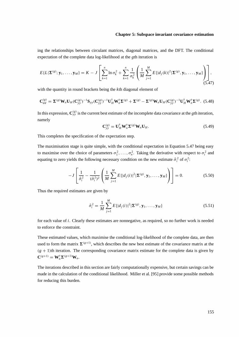
Chapter 5: Subspace invariant covariance estimation
ing the relationships between circulant matrices, diagonal matrices, and the DFT. The conditional
expectation of the complete data log-likelihood at the gth iteration is
E{L|6(g); y1, . . . , yM} = K − J
n∑
k=1
ln σ 2k +
n∑
k=1
1
σ 2k
1
M
M∑
j=1
E{|d j(k)|2|6(g), y1, . . . , yM}
,
(5.47)
with the quantity in round brackets being the kth diagonal element of
C(g)
dd = 6(g)WnUH(C(g)yy )−1Syy(C(g)
yy )−1U†H W†
n6(g) + 6(g) − 6(g)WnUH(C(g)
yy )−1U†H W†
n6(g). (5.48)
In this expression, C(g)yy is the current best estimate of the incomplete data covariance at the gth iteration,
namely
C(g)yy = U†
H W†n6
(g)WnUH . (5.49)
This completes the specification of the expectation step.
The maximisation stage is quite simple, with the conditional expectation in Equation 5.47 being easy
to maximise over the choice of parameters σ 21 , . . . , σ 2
n . Taking the derivative with respect to σ 2i and
equating to zero yields the following necessary condition on the new estimate σ 2i of σ 2
i :
−J
1
σ 2i
− 1
(σ 2i )2
1
M
M∑
j=1
E{|d j(i)|2|6(g), y1, . . . , yM}
= 0. (5.50)
Thus the required estimates are given by
σ 2i = 1
M
M∑
j=1
E{|d j(i)|2|6(g), y1, . . . , yM} (5.51)
for each value of i . Clearly these estimates are nonnegative, as required, so no further work is needed
to enforce the constraint.
These estimated values, which maximise the conditional log-likelihood of the complete data, are then
used to form the matrix 6(g+1), which describes the new best estimate of the covariance matrix at the
(g + 1)th iteration. The corresponding covariance matrix estimate for the complete data is given by
C(g+1) = W†n6
(g+1)Wn.
The iterations described in this section are fairly computationally expensive, but certain savings can be
made in the calculation of the conditional likelihood. Miller et al. [95] provide some possible methods
for reducing this burden.
155
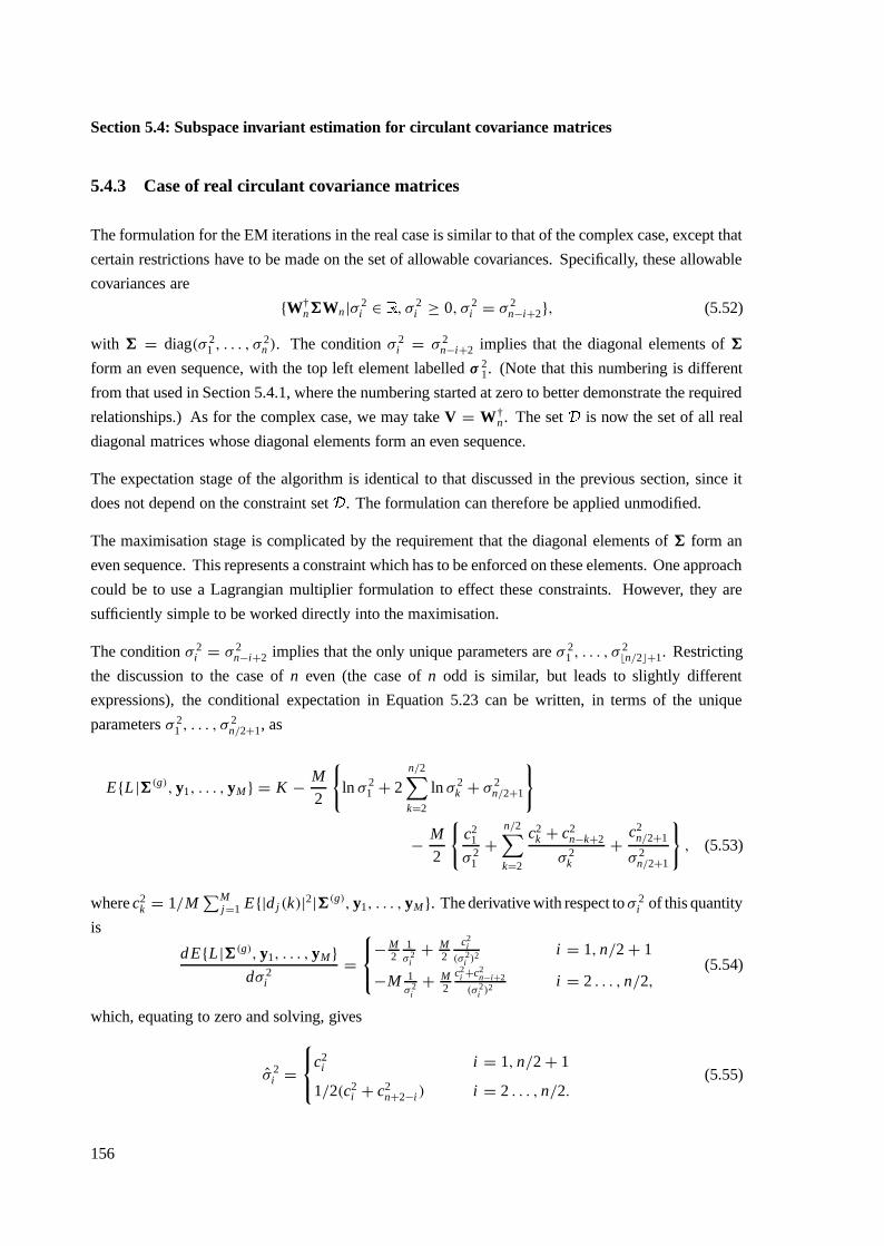
Section 5.4: Subspace invariant estimation for circulant covariance matrices
5.4.3 Case of real circulant covariance matrices
The formulation for the EM iterations in the real case is similar to that of the complex case, except that
certain restrictions have to be made on the set of allowable covariances. Specifically, these allowable
covariances are
{W†n6Wn|σ 2
i ∈ �, σ 2
i ≥ 0, σ 2i = σ 2
n−i+2}, (5.52)
with 6 = diag(σ 21 , . . . , σ 2
n ). The condition σ 2i = σ 2
n−i+2 implies that the diagonal elements of 6
form an even sequence, with the top left element labelled σ 21. (Note that this numbering is different
from that used in Section 5.4.1, where the numbering started at zero to better demonstrate the required
relationships.) As for the complex case, we may take V = W†n . The set
�is now the set of all real
diagonal matrices whose diagonal elements form an even sequence.
The expectation stage of the algorithm is identical to that discussed in the previous section, since it
does not depend on the constraint set�
. The formulation can therefore be applied unmodified.
The maximisation stage is complicated by the requirement that the diagonal elements of 6 form an
even sequence. This represents a constraint which has to be enforced on these elements. One approach
could be to use a Lagrangian multiplier formulation to effect these constraints. However, they are
sufficiently simple to be worked directly into the maximisation.
The condition σ 2i = σ 2
n−i+2 implies that the only unique parameters are σ 21 , . . . , σ 2
bn/2c+1. Restricting
the discussion to the case of n even (the case of n odd is similar, but leads to slightly different
expressions), the conditional expectation in Equation 5.23 can be written, in terms of the unique
parameters σ 21 , . . . , σ 2
n/2+1, as
E{L|6(g), y1, . . . , yM} = K − M
2
{ln σ 2
1 + 2n/2∑
k=2
ln σ 2k + σ 2
n/2+1
}
− M
2
{c2
1
σ 21
+n/2∑
k=2
c2k + c2
n−k+2
σ 2k
+c2
n/2+1
σ 2n/2+1
}, (5.53)
where c2k = 1/M
∑Mj=1 E{|d j(k)|2|6(g), y1, . . . , yM}. The derivative with respect to σ 2
i of this quantity
is
d E{L|6(g), y1, . . . , yM}dσ 2
i
=
− M2
1σ 2
i+ M
2c2
i
(σ 2i )2 i = 1, n/2 + 1
−M 1σ 2
i+ M
2c2
i +c2n−i+2
(σ 2i )2 i = 2 . . . , n/2,
(5.54)
which, equating to zero and solving, gives
σ 2i =
c2i i = 1, n/2 + 1
1/2(c2i + c2
n+2−i ) i = 2 . . . , n/2.(5.55)
156

Chapter 5: Subspace invariant covariance estimation
As with the previous case, these parameters can easily be calculated from the matrix C(g)
dd . Again these
estimates are clearly nonnegative, as required. They can be used directly as the elements of the best
estimate 6(g+1) of 6 at the (g + 1)th iteration.
Less apparent is the fact that the exact same algorithm can be used for this real case as for the complex
case, as long as the initial covariance estimate is real and symmetric. In order to see this, consider the
quantity C(g)
dd in Equation 5.48: using the relation C(g) = W†n6
(g)Wn, this can be written as
C(g)
dd = Wn[C(g)UH(C(g)yy )−1Syy(C(g)
yy )−1UTH C(g)]W†
n + 6(g)
− Wn[C(g)UH(C(g)yy )−1UT
H C(g)]W†n. (5.56)
Noting that the quantities in square brackets are both symmetric, the argument presented in Section 5.4.1
demonstrates that the first and last terms in this expression have diagonal elements which form an even
sequence. Therefore, if we have σ 2i = σ 2
n+i+2, then the elements of C(g)
dd are such that C(g)
dd (k, k) =C(g)
dd (n − k + 2, n − k + 2). Thus the form of the new parameter estimate 6 (g+1) is such that C(g+1) is
real and symmetric, as required.
5.4.4 Example of invariant circulant covariance estimation
Some results of applying the invariant constrained covariance matrix estimation procedure to three
different real-valued observations are provided in this section. The results assume that only a single
noise observation is available for the estimation, so M = 1. The samples were generated from ideal
zero-mean normal random processes. In each case the actual covariance matrix of the process was
chosen to be circulant, but with different correlation properties. The relevant autocorrelation functions
for the processes are demonstrated in Figure 5.2. Since the covariance matrices of the processes
0 10 20 30 40 50 600
0.2
0.4
0.6
0.8
1
Lag
Cor
rela
tion
prod
uct
acf 1acf 2acf 3
Figure 5.2: Autocorrelation functions for the three different processes used to generatethe samples for testing the circulant constrained invariant estimation.
157
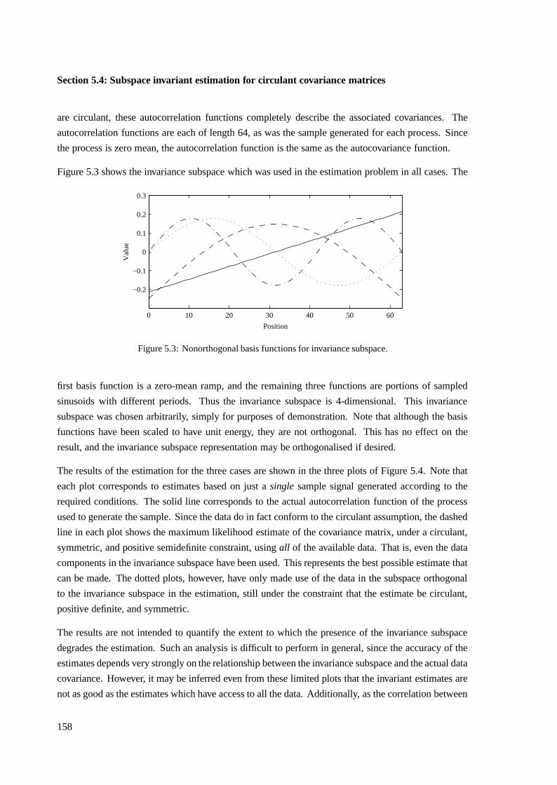
Section 5.4: Subspace invariant estimation for circulant covariance matrices
are circulant, these autocorrelation functions completely describe the associated covariances. The
autocorrelation functions are each of length 64, as was the sample generated for each process. Since
the process is zero mean, the autocorrelation function is the same as the autocovariance function.
Figure 5.3 shows the invariance subspace which was used in the estimation problem in all cases. The
0 10 20 30 40 50 60
−0.2
−0.1
0
0.1
0.2
0.3
Position
Val
ue
Figure 5.3: Nonorthogonal basis functions for invariance subspace.
first basis function is a zero-mean ramp, and the remaining three functions are portions of sampled
sinusoids with different periods. Thus the invariance subspace is 4-dimensional. This invariance
subspace was chosen arbitrarily, simply for purposes of demonstration. Note that although the basis
functions have been scaled to have unit energy, they are not orthogonal. This has no effect on the
result, and the invariance subspace representation may be orthogonalised if desired.
The results of the estimation for the three cases are shown in the three plots of Figure 5.4. Note that
each plot corresponds to estimates based on just a single sample signal generated according to the
required conditions. The solid line corresponds to the actual autocorrelation function of the process
used to generate the sample. Since the data do in fact conform to the circulant assumption, the dashed
line in each plot shows the maximum likelihood estimate of the covariance matrix, under a circulant,
symmetric, and positive semidefinite constraint, using all of the available data. That is, even the data
components in the invariance subspace have been used. This represents the best possible estimate that
can be made. The dotted plots, however, have only made use of the data in the subspace orthogonal
to the invariance subspace in the estimation, still under the constraint that the estimate be circulant,
positive definite, and symmetric.
The results are not intended to quantify the extent to which the presence of the invariance subspace
degrades the estimation. Such an analysis is difficult to perform in general, since the accuracy of the
estimates depends very strongly on the relationship between the invariance subspace and the actual data
covariance. However, it may be inferred even from these limited plots that the invariant estimates are
not as good as the estimates which have access to all the data. Additionally, as the correlation between
158
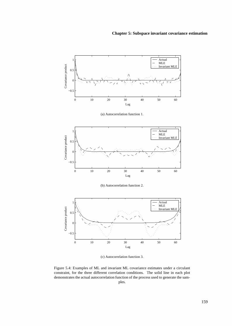
Chapter 5: Subspace invariant covariance estimation
0 10 20 30 40 50 60
−0.5
0
0.5
1
Lag
Cov
aria
nce
prod
uct Actual
MLE Invariant MLE
(a) Autocorrelation function 1.
0 10 20 30 40 50 60
−0.5
0
0.5
1
Lag
Cov
aria
nce
prod
uct Actual
MLE Invariant MLE
(b) Autocorrelation function 2.
0 10 20 30 40 50 60
−0.5
0
0.5
1
Lag
Cov
aria
nce
prod
uct Actual
MLE Invariant MLE
(c) Autocorrelation function 3.
Figure 5.4: Examples of ML and invariant ML covariance estimates under a circulantconstraint, for the three different correlation conditions. The solid line in each plotdemonstrates the actual autocorrelation function of the process used to generate the sam-
ples.
159
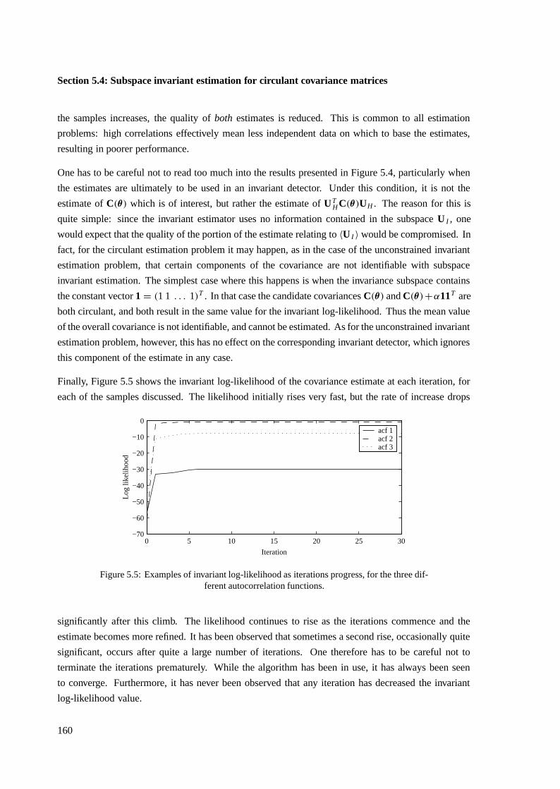
Section 5.4: Subspace invariant estimation for circulant covariance matrices
the samples increases, the quality of both estimates is reduced. This is common to all estimation
problems: high correlations effectively mean less independent data on which to base the estimates,
resulting in poorer performance.
One has to be careful not to read too much into the results presented in Figure 5.4, particularly when
the estimates are ultimately to be used in an invariant detector. Under this condition, it is not the
estimate of C(θ) which is of interest, but rather the estimate of UTH C(θ)UH . The reason for this is
quite simple: since the invariant estimator uses no information contained in the subspace U I , one
would expect that the quality of the portion of the estimate relating to 〈U I 〉 would be compromised. In
fact, for the circulant estimation problem it may happen, as in the case of the unconstrained invariant
estimation problem, that certain components of the covariance are not identifiable with subspace
invariant estimation. The simplest case where this happens is when the invariance subspace contains
the constant vector 1 = (1 1 . . . 1)T . In that case the candidate covariances C(θ) and C(θ)+α11T are
both circulant, and both result in the same value for the invariant log-likelihood. Thus the mean value
of the overall covariance is not identifiable, and cannot be estimated. As for the unconstrained invariant
estimation problem, however, this has no effect on the corresponding invariant detector, which ignores
this component of the estimate in any case.
Finally, Figure 5.5 shows the invariant log-likelihood of the covariance estimate at each iteration, for
each of the samples discussed. The likelihood initially rises very fast, but the rate of increase drops
0 5 10 15 20 25 30−70
−60
−50
−40
−30
−20
−10
0
Iteration
Log
likel
ihoo
d
acf 1acf 2acf 3
Figure 5.5: Examples of invariant log-likelihood as iterations progress, for the three dif-ferent autocorrelation functions.
significantly after this climb. The likelihood continues to rise as the iterations commence and the
estimate becomes more refined. It has been observed that sometimes a second rise, occasionally quite
significant, occurs after quite a large number of iterations. One therefore has to be careful not to
terminate the iterations prematurely. While the algorithm has been in use, it has always been seen
to converge. Furthermore, it has never been observed that any iteration has decreased the invariant
log-likelihood value.
160
Chapter 5: Subspace invariant covariance estimation
5.5 Subspace invariant estimation for Toeplitz covariance matrices
In this section, the previous results are extended to the problem of covariance matrix estimation under
a Toeplitz constraint, both with and without an invariance subspace. Initially, the case of no invariance
is considered, since it is slightly simpler to explain. This case is fairly extensively discussed in the
literature, usually as applied to complex observations and covariances. Once the simpler case has been
discussed, extending the results to include an invariance subspace is easy.
5.5.1 Estimation without subspace invariance
The standard approach to estimating covariance matrices under a Toeplitz constraint is to once again
use a missing data interpretation. The relationship between the complete and incomplete data is of a
very specific form: each observed data vector xi is assumed to consist of the first n elements of an
hypothetical s-dimensional complete data vector ui , which is MVN with an unknown positive definite
circulant covariance matrix. The vectors x1, . . . , xM play the role of the incomplete data in the EM
formulation. The relationship between xi and ui is therefore
xi =(
In×n 0)
ui , (5.57)
where In×n is the n × n identity matrix, and 0 is a matrix of zeros of the appropriate order. This
transformation simply extract the first n elements of ui .
The approach used for the estimation makes use of the observation that the top-left block of a cir-
culant matrix has a Toeplitz structure. Furthermore, if the matrix is positive semidefinite, then the
corresponding block is also positive semidefinite. Explicitly, if C is circulant and positive definite,
then (In×n 0
)C
(In×n
0
)(5.58)
is positive semidefinite and Toeplitz. Noting that this matrix is precisely the covariance of x i if
ui : N [0, C], it is apparent that maximising the likelihood subject to a circulant constraint on the
complete data will result in a Toeplitz estimate for the covariance matrix of the incomplete data.
A circulant positive definite Hermitian constraint on the complete data is therefore equivalent to a
Toeplitz positive definite Hermitian constraint on the incomplete data. What is not apparent, however,
is to what extent the converse is true: what proportion of n ×n Toeplitz matrices can be embedded into
the top-left block of a s × s circulant matrix? This is an important question, since it is over precisely
these matrices that the effective maximisation will be performed. Specifically, if the complete data
circulant covariance matrix is required to be Hermitian and positive definite, then the implied set of
161
Section 5.5: Subspace invariant estimation for Toeplitz covariance matrices
Toeplitz covariance matrices over which the incomplete data likelihood is maximised is precisely
{(In×n 0
)C
(In×n
0
)∣∣∣∣∣C is Hermitian, positive definite, and circulant
}. (5.59)
Evidently this is not exactly equivalent to the set of all positive definite Hermitian Toeplitz matrices
— the latter set contains elements not included in the former.
The extent to which the formulation is appropriate for the problem depends on the dimension chosen
for the complete data, namely the parameter s. This parameter is entirely free in the formulation, and
the only effect that it has is on the extent to which the implied constraint approximates the required
constraint. For example, if s is chosen to equal n, the effective constraint set is just the set of circulant
matrices with the required properties. The elements of this set satisfy the requirement that they be
Toeplitz (since a circulant matrix is always Toeplitz), but at the same time the set is far smaller than the
complete set of Toeplitz matrices. Thus a more stringent constraint has been placed on the candidate
covariances than was actually desired. As s is chosen successively larger than n, this disparity becomes
smaller. Dembo, Mallows, and Shepp [27] demonstrate that every finite-dimensional positive definite
Toeplitz matrix can be embedded into a circulant matrix of sufficiently large order. They also provide
bounds on s required for such an embedding, based on the value of the minimum eigenvalue of the
Toeplitz matrix.
In practice the difference between the actual constraint in force and the desired constraint appears not
to be critical. As long as s is fairly large relative to n (a factor of two seems acceptible), the resulting
estimates are reasonable and useful. However, it should be remembered that the estimate obtained may
in fact only be an approximation to what is required.
Returning to the formal development of the algorithm for implementing the estimation, as in the
previous section two cases have to be considered: real and of complex covariances. Each requires a
different specification of the constraint set. Once described, however, the development of the algorithm
details is straightforward.
For the case of complex covariances, the constraint on the complete data covariance C is that it be
Hermitian, positive semidefinite, and circulant. This is identical to the constraint used in Section 5.4.2,
so the choice of V = W†n and
�to be the set of all real diagonal matrices with nonnegative elements
is appropriate. The only difference is in the definition of the transformation matrix A. With the
incomplete data (v1, . . . , vM) taken to be the actual observations (x1, . . . , xM), and the complete data
u1, . . . , uM as described, the relationship provided in Equation 5.57 implies that
A =(
In×n 0)
. (5.60)
This completely specifies the required quantities in the EM formulation.
162

Chapter 5: Subspace invariant covariance estimation
The implementation details are fundamentally identical to those provided in the section on invariant
estimation for circulant matrices, although on account of the simple nature of the relationship between
the complete and incomplete data some computational simplifications may be included [95]. The only
difference is that now the incomplete data are taken to be the actual observations, rather than the data
contained in the valid subspace.
Similarly, the real case is essentially solved using the results of Section 5.4.3, with a similar set of
candidates for the complete data covariance C. Once again it may be observed that as long as the initial
estimate of the covariance is real and the observations are real, the algorithm for the solution to the
complex problem always results in real estimates for the covariance at the subsequent iteration. Thus
the two cases may be solved using the same implementation, by simply using an appropriate starting
condition.
Finally, some necessary conditions on the convergence of the EM algorithm are known [132], but it
is difficult to ascertain whether they are met for this Toeplitz covariance estimation problem [27]. In
practice it has been observed that it always seems to provide a good solution. Nevertheless, convergence
is sometimes quite slow, and the rate of increase in likelihood as the iterations progress is by no means
consistent. This can make it difficult to specify a stopping criterion for the iterations, especially if
accuracy is the dominant factor. For signal processing applications it may be reasonable to execute
a predetermined number of iterations to improve an estimate, particularly when execution time is a
constraint. Since the likelihood is nondecreasing, a fixed number of iterations will always provide a
better solution (in the maximum likelihood sense) than the original estimate.
5.5.2 Estimation with subspace invariance
With the generalised EM formulation presented in Section 5.3, the extension of the Toeplitz covari-
ance estimation problem to include subspace invariance is easily achieved. Suppose the observed data
are x1, . . . , xM , each assumed to nominally be normally distributed, with a zero mean and a Toeplitz
covariance matrix. These observations are corrupted by mismatch components in the invariance sub-
space 〈UI 〉. Thus the components yi , . . . , yM are all that can be considered valid for estimation, where
yi = UTH xi .
Conceptually, it is quite useful to postulate the hypothetical data z1, . . . , zM , which are identical to the
observed data x1, . . . , xM except that they have not been corrupted in the invariance subspace. Thus
zi actually does conform to the Toeplitz assumption. The sets of observations however may differ in
the invariance subspace, so all that can be guaranteed is that UTH zi = UT
H xi .
If z1, . . . , zM could actually be observed, the estimation of the Toeplitz covariance matrix could be
achieved using the results of the previous section. In particular, the s-dimensional complete data vectors
u1, . . . , uM are proposed, which have a circulant covariance matrix C. The relationship between these
163
Section 5.5: Subspace invariant estimation for Toeplitz covariance matrices
complete data and the hypothetical ideal uncorrupted observations z1, . . . , zM is
zi =(
In×n 0)
ui . (5.61)
These uncorrupted observations are not observed: all that can be considered observable are the com-
ponents in the subspace orthogonal to the invariance subspace, namely UTH z1, . . . , UT
H zM . These quite
naturally take the role of the incomplete data observations in the EM formulation. It is required to
maximise the log-likelihood of these incomplete data observations over the complete data covariance
matrix C. Once this estimate is obtained, the required Toeplitz covariance matrix is
(In×n 0
)C
(In×n
0
). (5.62)
Now, the observable components UTH z1, . . . , UT
H zM are precisely y1, . . . , yM , which can therefore be
considered the incomplete data.
With these quantities all specified, it is easy to establish the relationship between the complete data
u1, . . . , uM and the incomplete data y1, . . . , yM :
yi = UTH xi = UT
H zi = UTH
(In×n 0
)ui . (5.63)
Thus for the EM algorithm, it is appropriate to take
A = UTH
(In×n 0
). (5.64)
The constraint sets for the complex and real cases are chosen exactly as in the previous discussion,
and the form of the quantities to be calculated in the iterations is identical. That is, the conditional
expectation of the complete data log-likelihood is
L(6; d1, . . . , dM) = K − J
s∑
k=1
ln σ 2k + 1
M
M∑
j=1
s∑
k=1
|d j (k)|2σ 2
k
, (5.65)
which can be calculated using the diagonal elements of
C(g)
dd = 6(g)V†A†(C(g)yy )−1Syy(C(g)
yy )−1AV6(g) + 6(g) − 6(g)V†A†(C(g)yy )−1AV6(g)
= 6(g)Wn
(In×n
0
)UH(C(g)
yy )−1Syy(C(g)yy )−1U†
H
(In×n 0
)W†
n6(g) + 6(g) (5.66)
− 6(g)Wn
(In×n
0
)UH(C(g)
yy )−1U†H
(In×n 0
)W†
n6(g), (5.67)
164
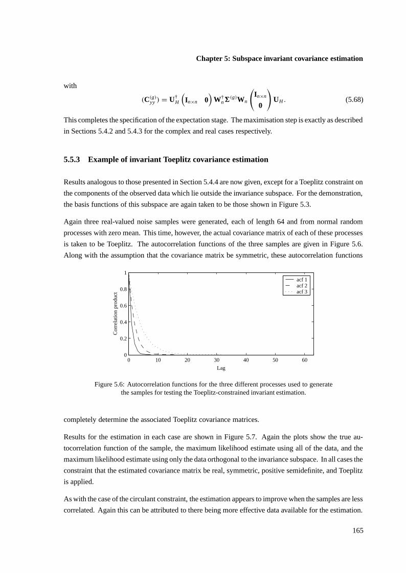
Chapter 5: Subspace invariant covariance estimation
with
(C(g)yy ) = U†
H
(In×n 0
)W†
n6(g)Wn
(In×n
0
)UH . (5.68)
This completes the specification of the expectation stage. The maximisation step is exactly as described
in Sections 5.4.2 and 5.4.3 for the complex and real cases respectively.
5.5.3 Example of invariant Toeplitz covariance estimation
Results analogous to those presented in Section 5.4.4 are now given, except for a Toeplitz constraint on
the components of the observed data which lie outside the invariance subspace. For the demonstration,
the basis functions of this subspace are again taken to be those shown in Figure 5.3.
Again three real-valued noise samples were generated, each of length 64 and from normal random
processes with zero mean. This time, however, the actual covariance matrix of each of these processes
is taken to be Toeplitz. The autocorrelation functions of the three samples are given in Figure 5.6.
Along with the assumption that the covariance matrix be symmetric, these autocorrelation functions
0 10 20 30 40 50 600
0.2
0.4
0.6
0.8
1
Lag
Cor
rela
tion
prod
uct
acf 1acf 2acf 3
Figure 5.6: Autocorrelation functions for the three different processes used to generatethe samples for testing the Toeplitz-constrained invariant estimation.
completely determine the associated Toeplitz covariance matrices.
Results for the estimation in each case are shown in Figure 5.7. Again the plots show the true au-
tocorrelation function of the sample, the maximum likelihood estimate using all of the data, and the
maximum likelihood estimate using only the data orthogonal to the invariance subspace. In all cases the
constraint that the estimated covariance matrix be real, symmetric, positive semidefinite, and Toeplitz
is applied.
As with the case of the circulant constraint, the estimation appears to improve when the samples are less
correlated. Again this can be attributed to there being more effective data available for the estimation.
165
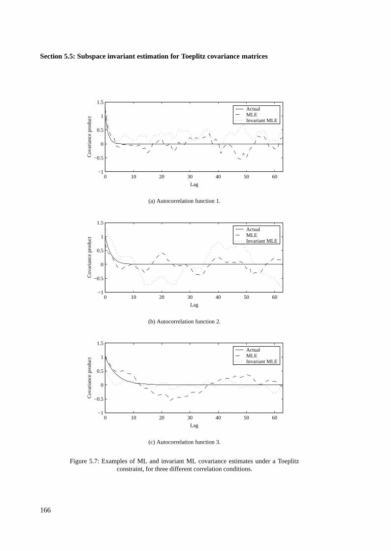
Section 5.5: Subspace invariant estimation for Toeplitz covariance matrices
0 10 20 30 40 50 60−1
−0.5
0
0.5
1
1.5
Lag
Cov
aria
nce
prod
uct Actual
MLE Invariant MLE
(a) Autocorrelation function 1.
0 10 20 30 40 50 60−1
−0.5
0
0.5
1
1.5
Lag
Cov
aria
nce
prod
uct Actual
MLE Invariant MLE
(b) Autocorrelation function 2.
0 10 20 30 40 50 60−1
−0.5
0
0.5
1
1.5
Lag
Cov
aria
nce
prod
uct Actual
MLE Invariant MLE
(c) Autocorrelation function 3.
Figure 5.7: Examples of ML and invariant ML covariance estimates under a Toeplitzconstraint, for three different correlation conditions.
166
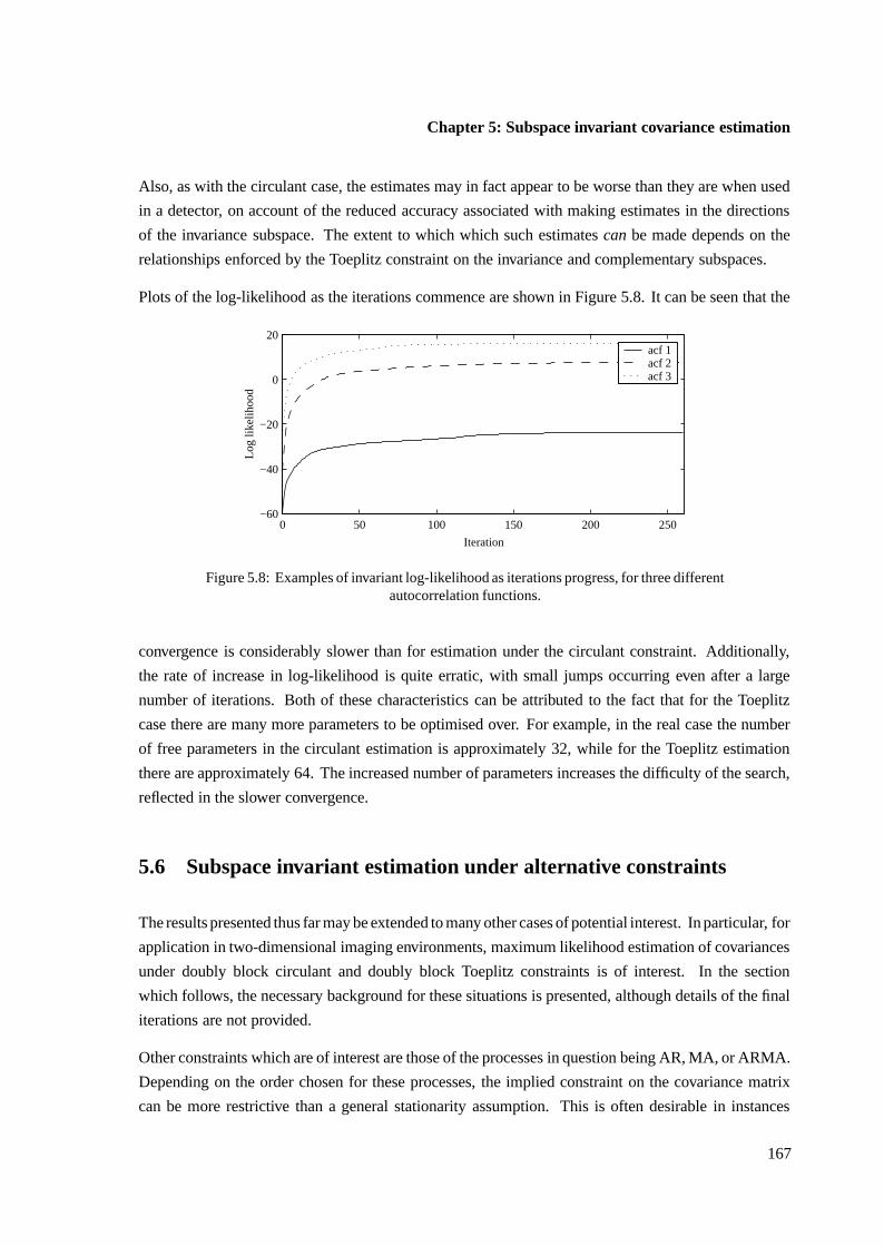
Chapter 5: Subspace invariant covariance estimation
Also, as with the circulant case, the estimates may in fact appear to be worse than they are when used
in a detector, on account of the reduced accuracy associated with making estimates in the directions
of the invariance subspace. The extent to which which such estimates can be made depends on the
relationships enforced by the Toeplitz constraint on the invariance and complementary subspaces.
Plots of the log-likelihood as the iterations commence are shown in Figure 5.8. It can be seen that the
0 50 100 150 200 250−60
−40
−20
0
20
Iteration
Log
likel
ihoo
d
acf 1acf 2acf 3
Figure 5.8: Examples of invariant log-likelihood as iterations progress, for three differentautocorrelation functions.
convergence is considerably slower than for estimation under the circulant constraint. Additionally,
the rate of increase in log-likelihood is quite erratic, with small jumps occurring even after a large
number of iterations. Both of these characteristics can be attributed to the fact that for the Toeplitz
case there are many more parameters to be optimised over. For example, in the real case the number
of free parameters in the circulant estimation is approximately 32, while for the Toeplitz estimation
there are approximately 64. The increased number of parameters increases the difficulty of the search,
reflected in the slower convergence.
5.6 Subspace invariant estimation under alternative constraints
The results presented thus far may be extended to many other cases of potential interest. In particular, for
application in two-dimensional imaging environments, maximum likelihood estimation of covariances
under doubly block circulant and doubly block Toeplitz constraints is of interest. In the section
which follows, the necessary background for these situations is presented, although details of the final
iterations are not provided.
Other constraints which are of interest are those of the processes in question being AR, MA, or ARMA.
Depending on the order chosen for these processes, the implied constraint on the covariance matrix
can be more restrictive than a general stationarity assumption. This is often desirable in instances
167

Section 5.6: Subspace invariant estimation under alternative constraints
where the amount of data available for estimation is small. As with the Toeplitz case, however, as far
as invariant detection is concerned it is useful to be able to make invariant estimates of the associated
parameter values. This case is discussed briefly in Section 5.6.2.
5.6.1 Doubly block circulant and doubly block Toeplitz constraints
A doubly block circulant matrix is a matrix which has a circulant block struture, each block of which
is circulant. A doubly block Toeplitz matrix is defined similarly. These matrices arise in statistical
characterisation of covariances of cyclic or stationary data, when 2-D observations are reordered into
a column vector through column or row ordering.
The constraints can also be cast into the form required by the general algorithm developed in Sec-
tion 5.3. The most difficult part of the formulation involves the diagonalisation of general doubly
block circulant matrices. This section begins with a description of how such matrices can be diago-
nalised in the complex case. The required quantities for specifying the EM iterations under doubly
circulant and doubly Toeplitz constraints are then provided. In the interests of simplicity only complex
matrix formulations are considered, and estimation with an invariance subspace is not presented. The
extensions are however quite simple, and conceptually follow the same procedures as for the simpler
cases of Toeplitz and circulant covariances.
Let B be a doubly block circulant matrix, with r × r blocks each of dimension s × s:
B =
C0 C1 C2 · · · Cr−1
Cr−1 C0 C1 · · · Cr−2...
......
. . ....
C1 C2 C3 · · · C0
, (5.69)
Note that B is in general itself not circulant.
Davis [24, p. 185] demonstrates the following points:
• B is diagonalisable by the unitary matrix Wr ⊗ Ws , where ⊗ is the Kronecker product op-
erator [49]. Furthermore, if the matrices of eigenvalues of the circulant blocks are given by
3k, k = 0, . . . , r −1, then the diagonal matrix of the eigenvalues of B is given by∑r−1
k=0 �kr ⊗3k .
In this expression, �r = diag(w−0r , w−1
r , . . . , w−(r−1)r ).
• Any matrix A = (Wr ⊗ Ws)3(Wr ⊗ Ws), where 3 is diagonal, is doubly block circulant, with
r × r blocks each of dimension s × s. Since (Wr ⊗ Ws) = (Wr ⊗ Ws)†, this can be written in
the more conventional form A = (Wr ⊗ Ws)†3(Wr ⊗ Ws).
These are analogous to the results provided for circulant matrices, and give necessary and sufficient
168
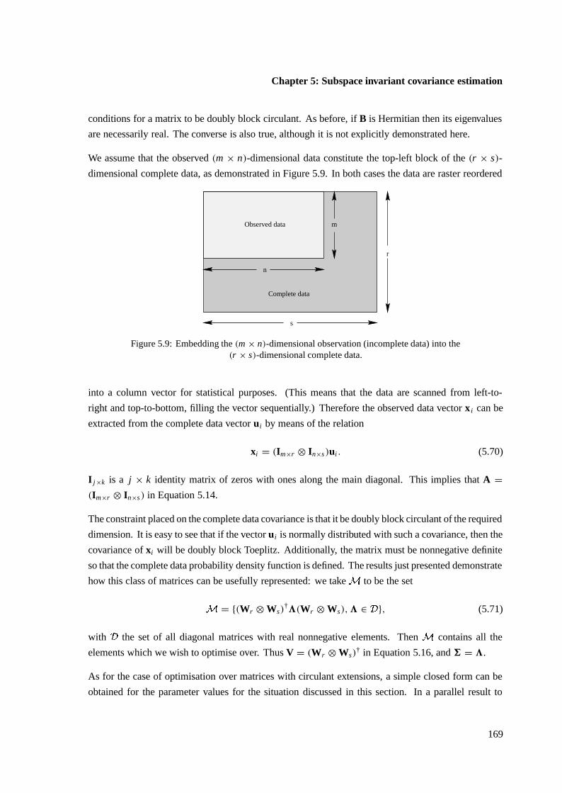
Chapter 5: Subspace invariant covariance estimation
conditions for a matrix to be doubly block circulant. As before, if B is Hermitian then its eigenvalues
are necessarily real. The converse is also true, although it is not explicitly demonstrated here.
We assume that the observed (m × n)-dimensional data constitute the top-left block of the (r × s)-
dimensional complete data, as demonstrated in Figure 5.9. In both cases the data are raster reordered
Complete data
n
s
Observed data
r
m
Figure 5.9: Embedding the (m × n)-dimensional observation (incomplete data) into the(r × s)-dimensional complete data.
into a column vector for statistical purposes. (This means that the data are scanned from left-to-
right and top-to-bottom, filling the vector sequentially.) Therefore the observed data vector x i can be
extracted from the complete data vector ui by means of the relation
xi = (Im×r ⊗ In×s)ui . (5.70)
I j×k is a j × k identity matrix of zeros with ones along the main diagonal. This implies that A =(Im×r ⊗ In×s) in Equation 5.14.
The constraint placed on the complete data covariance is that it be doubly block circulant of the required
dimension. It is easy to see that if the vector ui is normally distributed with such a covariance, then the
covariance of xi will be doubly block Toeplitz. Additionally, the matrix must be nonnegative definite
so that the complete data probability density function is defined. The results just presented demonstrate
how this class of matrices can be usefully represented: we take�
to be the set
� = {(Wr ⊗ Ws)†3(Wr ⊗ Ws),3 ∈ � }, (5.71)
with�
the set of all diagonal matrices with real nonnegative elements. Then�
contains all the
elements which we wish to optimise over. Thus V = (Wr ⊗ Ws)† in Equation 5.16, and 6 = 3.
As for the case of optimisation over matrices with circulant extensions, a simple closed form can be
obtained for the parameter values for the situation discussed in this section. In a parallel result to
169
Section 5.6: Subspace invariant estimation under alternative constraints
Equation 5.51,
σ 2i = 1
M
M∑
j=1
E{|d j(i)|2|6(g), x1, . . . , xM}, (5.72)
where all the relevant quantities have been derived from the raster reordered observations. For each i ,
this value is simply the i th diagonal element of C(g)
dd in Equation 5.31.
A final simplification arises by considering the value of the product V†A in the calculation. This
product is given by
V†A† = (Wr ⊗ Ws)(Im×r ⊗ In×s)†
= (Wr ⊗ Ws)(Ir×m ⊗ Is×n)
= Wr Ir×m ⊗ WsIs×n
= W(m)r ⊗ W(n)
s (5.73)
where W(m)r contains the first m columns of Wr , and W(n)
s contains the first n columns of Ws .
5.6.2 ARMA constraints
The final case of interest is that of subspace invariant estimation of covariance matrices under AR, MA,
and ARMA constraints. These are especially useful when the amount of data available for estimation
is small.
Even without the invariance subspace, maximum likelihood estimation for these models is difficult.
In most applications, approximations are used to simplify the objective likelihood function, which in
turn leads to an approximate maximum likelihood estimate. To some extent the estimation under an
autoregressive assumption is simpler than the cases of MA and ARMA processes, although it still does
not permit a convenient solution.
There are some fairly efficient methods available for calculating the likelihood of a general ARMA
process given a seqence of successive scalar observations. For example, an algorithm which finds this
likelihood using an innovations decomposition is provided by Mélard [94].
Unfortunately, it is difficult to use this type of approach within the EM framework presented in this
chapter. This is because the maximisation stage of the EM iteration, at least in the form presented,
requires a way of estimating the ARMA parameters from the conditional expectation of the sample
covariance matrix, rather than from a single sequence of observed values. Exact likelihood methods
for this problem are difficult to obtain, and Porat [104, p. 200] recommends simplifying the problem
through appropriate approximate methods. However, this casts the EM procedure in doubt, and since
a nondecreasing likelihood can no longer be guaranteed, convergence may not occur with a modified
170

Chapter 5: Subspace invariant covariance estimation
estimate. Unfortunately the EM method does not appear to permit an alternative formulation, where
this problem is overcome.
For this reason, a simpler approach is to maximise the invariant log-likelihood function directly, over
the space of allowed parameter values for the general ARMA process. Computationally this is an
expensive procedure, but is sufficient as far as investigating ideas is concerned. Furthermore, since
the number of parameters in the models is generally low, search methods are not unreasonable for the
estimation. Thus, where required, the invariant log-likelihood is simply maximised using the Nelder-
Mead simplex algorithm [108]. The matrices over which this maximisation is performed is the set of
all possible valid covariance matrices of the assumed process. The set of parameter values is chosen
such that the implied ARMA process is stable and invertible. Kay [75, p. 131] provides a method
of calculating the autocorrelation function of an ARMA process, which is all that is required in the
likelihood calculation.
5.7 Simultaneous estimation of interference subspace and covariance
matrix
Chapter 4 discussed the problem of estimating the invariance subspace from actual data, when the true
covariance matrix is known. Chapter 5 discussed the dual problem of estimating the covariance matrix
when the invariance subspace is known. A problem which has not yet been addressed is how to make
simultaneous estimates of these two quantities when neither are known.
This is a difficult problem, for which no ideal solution has been found. For the interference subspace
estimate, the primary cause of this difficulty is the fact that the proposed estimation method is only
approximate, with no maximum likelihood solution having been obtained. For the invariance subspace
in the model mismatch problem, the difficulty arises in that an estimate is obtained of the invariance
subspace, and not of the complementary subspace.
One method which presents itself is to iterate between the invariance subspace estimation and the
covariance matrix estimation, in the hope that the procedure will converge to a reasonable solution for
both quantities. There is no guarantee that this method will provide a good solution set, however. In
fact, it is difficult to determine whether the procedure will even converge. In some cases it has been
seen to provide a reasonable solution, but this is difficult to validate in general.
At least for the subspace interference problem, a better solution is to attempt to maximise the likelihood
over both the unknown covariance matrix and the unknown invariance subspace. Thus the invariant
likelihood should be maximised over the joint parameters U I (or equivalently UH ) and C. Since the
value of UH that approximately maximises this likelihood is known with respect to C, the explicit
dependence on UH can be eliminated: we know UH(θ), where θ parameterises the covariance matrix.
171
Section 5.7: Simultaneous estimation of interference subspace and covariance matrix
An approximate modified invariant likelihood can therefore be formulated as
La = (2π)−M(n−p)/2|UTH(θ)C(θ)UH(θ)|−M/2e− 1
2∑M
j=1 yTj (UT
H (θ)C(θ)UH (θ))−1y j . (5.74)
Maximising over θ then yields the approximate covariance estimate, from which the corresponding
invariance subspace estimate can be obtained.
Unfortunately this procedure can only be applied using direct maximisation over the parameter θ .
The invariant covariance estimates for circulant and Toeplitz matrices cannot be used in this context,
since they require that the invariance subspace be held constant over the maximisation. Nevertheless,
estimates using ARMA processes can be obtained, by adopting the search methods described in the
previous section.
To demonstrate the performance of this proposed procedure for the subspace interference case, the
experiment presented in Section 4.3.6 was repeated. Data samples were again generated from first-
order AR processes with autocorrelation functions shown in Figure 4.7, and subspace interference
added as before. This time the underlying covariance matrix, which generated the samples prior to
interference being added, was not assumed known. Instead, under just the assumption of a first-order
autoregressive model, the procedure outlined in this section was used.
As for the earlier case, this interference subspace estimation procedure was repeated 100 times for
each set of parameters of interest. Figure 5.10 shows the results of the simulations, and is analogous to
the results in Figure 4.8 for the known covariance case. The performance of the proposed procedure
is good, and indicates that the fact that the covariance matrix is unknown has a negligible effect on the
accuracy of the interference subspace estimates.
It must be noted that the assumption of a first-order autoregressive process was completely appropriate
and valid for the results presented. In general this may not be the case, and it is difficult to predict the
effect on the algorithm if the assumed model is invalid. Also, the model used has only two degrees of
freedom. For estimating the parameters of this model, the 50 or 200 noise samples represent a huge
amount of data on which to base these estimates. It is therefore not surprising that the covariance
matrix and interference subspace estimates are good.
If assumptions of more general covariance structures are required, a reasonable approach would be to
estimate the interference subspace using the method just described, using an ARMA process of fairly
high order. Once estimated, the invariance subspace can be held fixed while an invariant Toeplitz or
circulant constrained covariance matrix estimate is made. Although not ideal, if the ARMA process
is sufficiently flexible, the interference subspace estimate will be fairly accurate. At the very least, the
main causes of nonstationarity will have been eliminated.
For the case of subspace invariance for model mismatch, the same procedure can be used. This
time, however, the relationship between the invariance subspace estimate and the covariance matrix is
172
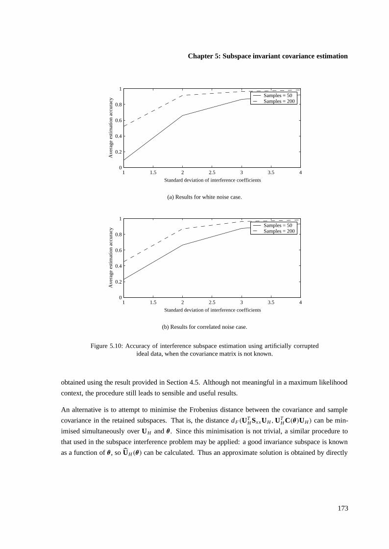
Chapter 5: Subspace invariant covariance estimation
1 1.5 2 2.5 3 3.5 40
0.2
0.4
0.6
0.8
1
Standard deviation of interference coefficients
Ave
rage
est
imat
ion
accu
racy
Samples = 50 Samples = 200
(a) Results for white noise case.
1 1.5 2 2.5 3 3.5 40
0.2
0.4
0.6
0.8
1
Standard deviation of interference coefficients
Ave
rage
est
imat
ion
accu
racy
Samples = 50 Samples = 200
(b) Results for correlated noise case.
Figure 5.10: Accuracy of interference subspace estimation using artificially corruptedideal data, when the covariance matrix is not known.
obtained using the result provided in Section 4.5. Although not meaningful in a maximum likelihood
context, the procedure still leads to sensible and useful results.
An alternative is to attempt to minimise the Frobenius distance between the covariance and sample
covariance in the retained subspaces. That is, the distance dF(UTH Sx xUH , UT
H C(θ)UH) can be min-
imised simultaneously over UH and θ . Since this minimisation is not trivial, a similar procedure to
that used in the subspace interference problem may be applied: a good invariance subspace is known
as a function of θ , so UH(θ) can be calculated. Thus an approximate solution is obtained by directly
173
Section 5.8: Practical examples of invariant detectors
minimising the modified distance measure
dF(UTH(θ)Sx xUH(θ), UT
H(θ)C(θ)UH(θ)) =tr{UT
H(θ)(Sx x − C(θ))UH(θ)UTH(θ)(Sx x − C(θ))UH(θ)
}(5.75)
with respect to θ .
5.8 Practical examples of invariant detectors
The primary justification for invariant detectors is to eliminate the effect of subspace interference or low-
rank model mismatch from the detection problem. The invariant detector ignores these components,
thereby gaining a potential performance advantage via improved modelling.
A useful characteristic of the invariant detector is that it achieves this improved accuracy without
the need for adaptivity. This facilitates the calculation of the detection statistic, and is useful in
environments where speed is critical. Ideally, if the invariance subspace is correctly identified, the
resulting detector will be robust to the types of interference or model mismatch which commonly
occur.
In this section, it is shown how an invariant detector can improve overall performance in the case of
certain real-data applications. To make a fair assessment, it is necessary to clarify the characteristics
that a good detector should have. Firstly, the detection statistic should be highly discriminatory: that
is, it should differ maximally under the conditions of target absence and target presence. However, in
most cases this is not sufficient to define a good detector. Just as important, is the requirement that the
values which the statistic take on under the various hypotheses be consistent and well characterised.
At some point a decision has to be made based on the value of the detection statistic; if this decision
cannot be made meaningfully, the detector is useless in practice.
5.8.1 Invariance subspace for interference
The first example uses real samples of data, and attempts to assess whether the noise plus subspace
interference assumption can be successfully used to model the data for purposes of detection. In partic-
ular, subspace interference of various dimensionalities is assumed to be present in the observations, and
simultaneous estimates are obtained of the interference subspaces and covariance matrix parameters.
A highly-constrained covariance model is initially assumed, namely that of a first-order autoregressive
process, so the procedure presented in Section 5.7 for the estimation is appropriate.
Two samples of data were used, extracted from disjoint regions in an x-ray image of a human torso.
174
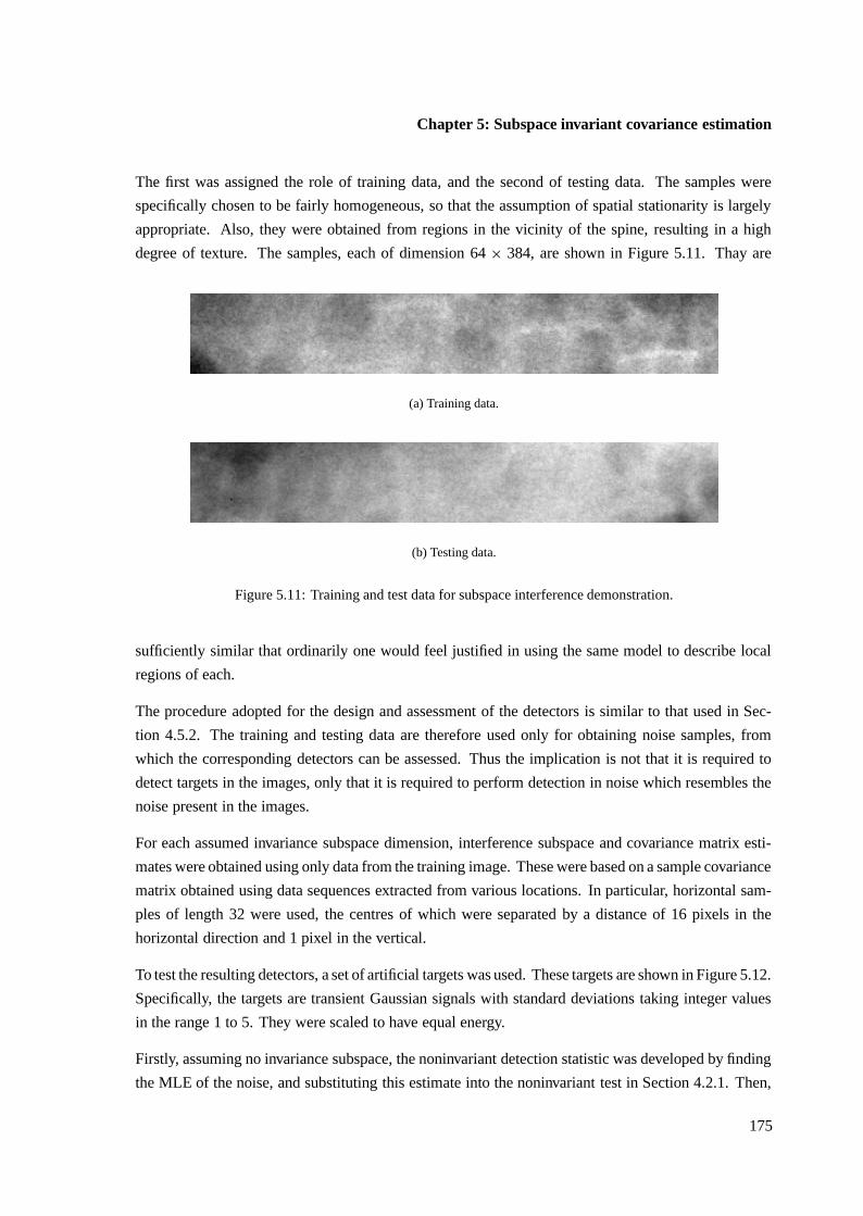
Chapter 5: Subspace invariant covariance estimation
The first was assigned the role of training data, and the second of testing data. The samples were
specifically chosen to be fairly homogeneous, so that the assumption of spatial stationarity is largely
appropriate. Also, they were obtained from regions in the vicinity of the spine, resulting in a high
degree of texture. The samples, each of dimension 64 × 384, are shown in Figure 5.11. Thay are
(a) Training data.
(b) Testing data.
Figure 5.11: Training and test data for subspace interference demonstration.
sufficiently similar that ordinarily one would feel justified in using the same model to describe local
regions of each.
The procedure adopted for the design and assessment of the detectors is similar to that used in Sec-
tion 4.5.2. The training and testing data are therefore used only for obtaining noise samples, from
which the corresponding detectors can be assessed. Thus the implication is not that it is required to
detect targets in the images, only that it is required to perform detection in noise which resembles the
noise present in the images.
For each assumed invariance subspace dimension, interference subspace and covariance matrix esti-
mates were obtained using only data from the training image. These were based on a sample covariance
matrix obtained using data sequences extracted from various locations. In particular, horizontal sam-
ples of length 32 were used, the centres of which were separated by a distance of 16 pixels in the
horizontal direction and 1 pixel in the vertical.
To test the resulting detectors, a set of artificial targets was used. These targets are shown in Figure 5.12.
Specifically, the targets are transient Gaussian signals with standard deviations taking integer values
in the range 1 to 5. They were scaled to have equal energy.
Firstly, assuming no invariance subspace, the noninvariant detection statistic was developed by finding
the MLE of the noise, and substituting this estimate into the noninvariant test in Section 4.2.1. Then,
175

Section 5.8: Practical examples of invariant detectors
5 10 15 20 25 300
20
40
60
80
100
120
140Target 1Target 2Target 3Target 4Target 5
Figure 5.12: Targets used for testing the invariant detection.
for assumed interference subspace dimensions from 1 to 10, the covariance matrix and interference
subspace estimates described earlier were obtained, and simply plugged into the subspace invariant
test statistic of Equation 4.2.2. Figure 5.13 shows an example of the effective detection templates
corresponding to noninvariant and invariant tests, for one specific target and interference subspace
dimension.
0 5 10 15 20 25 30 35−0.6
−0.4
−0.2
0
0.2
0.4
0.6Noninvariant templateInvariant template
Figure 5.13: Effective templates for noninvariant and invariant detection of Target 3. Thisresult is for an invariance subspace of dimension 4.
Using the methods described, 11 detection statistics, 11 covariance matrix estimates, and 10 invariance
subspace estimates (since there is no estimate for the noninvariant test) were obtained. Each of these
detection statistics was then applied to noise samples taken from both the training and the testing data,
and independent sets of results were formed. Additionally, targets were added to the noise samples,
simulating conditions of target presence, and the detection statistics were again calculated.
Table 5.1 shows the average normalised separation between the sets of values taken on by the test
statistics under the conditions of target absence and target presence. That is, the absolute difference
176
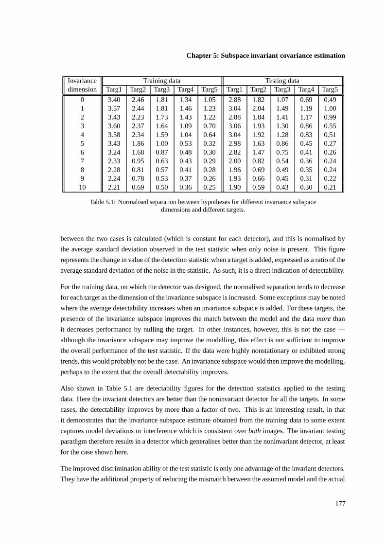
Chapter 5: Subspace invariant covariance estimation
Invariance Training data Testing datadimension Targ1 Targ2 Targ3 Targ4 Targ5 Targ1 Targ2 Targ3 Targ4 Targ5
0 3.40 2.46 1.81 1.34 1.05 2.88 1.82 1.07 0.69 0.491 3.57 2.44 1.81 1.46 1.23 3.04 2.04 1.49 1.19 1.002 3.43 2.23 1.73 1.43 1.22 2.88 1.84 1.41 1.17 0.993 3.60 2.37 1.64 1.09 0.70 3.06 1.93 1.30 0.86 0.554 3.58 2.34 1.59 1.04 0.64 3.04 1.92 1.28 0.83 0.515 3.43 1.86 1.00 0.53 0.32 2.98 1.63 0.86 0.45 0.276 3.24 1.68 0.87 0.48 0.30 2.82 1.47 0.75 0.41 0.267 2.33 0.95 0.63 0.43 0.29 2.00 0.82 0.54 0.36 0.248 2.28 0.81 0.57 0.41 0.28 1.96 0.69 0.49 0.35 0.249 2.24 0.78 0.53 0.37 0.26 1.93 0.66 0.45 0.31 0.22
10 2.21 0.69 0.50 0.36 0.25 1.90 0.59 0.43 0.30 0.21
Table 5.1: Normalised separation between hypotheses for different invariance subspacedimensions and different targets.
between the two cases is calculated (which is constant for each detector), and this is normalised by
the average standard deviation observed in the test statistic when only noise is present. This figure
represents the change in value of the detection statistic when a target is added, expressed as a ratio of the
average standard deviation of the noise in the statistic. As such, it is a direct indication of detectability.
For the training data, on which the detector was designed, the normalised separation tends to decrease
for each target as the dimension of the invariance subspace is increased. Some exceptions may be noted
where the average detectability increases when an invariance subspace is added. For these targets, the
presence of the invariance subspace improves the match between the model and the data more than
it decreases performance by nulling the target. In other instances, however, this is not the case —
although the invariance subspace may improve the modelling, this effect is not sufficient to improve
the overall performance of the test statistic. If the data were highly nonstationary or exhibited strong
trends, this would probably not be the case. An invariance subspace would then improve the modelling,
perhaps to the extent that the overall detectability improves.
Also shown in Table 5.1 are detectability figures for the detection statistics applied to the testing
data. Here the invariant detectors are better than the noninvariant detector for all the targets. In some
cases, the detectability improves by more than a factor of two. This is an interesting result, in that
it demonstrates that the invariance subspace estimate obtained from the training data to some extent
captures model deviations or interference which is consistent over both images. The invariant testing
paradigm therefore results in a detector which generalises better than the noninvariant detector, at least
for the case shown here.
The improved discrimination ability of the test statistic is only one advantage of the invariant detectors.
They have the additional property of reducing the mismatch between the assumed model and the actual
177
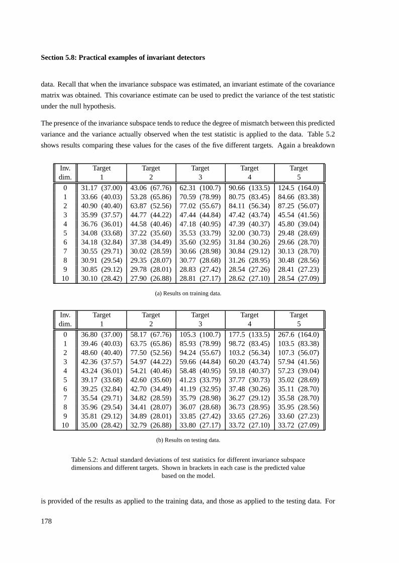
Section 5.8: Practical examples of invariant detectors
data. Recall that when the invariance subspace was estimated, an invariant estimate of the covariance
matrix was obtained. This covariance estimate can be used to predict the variance of the test statistic
under the null hypothesis.
The presence of the invariance subspace tends to reduce the degree of mismatch between this predicted
variance and the variance actually observed when the test statistic is applied to the data. Table 5.2
shows results comparing these values for the cases of the five different targets. Again a breakdown
Inv. Target Target Target Target Targetdim. 1 2 3 4 5
0 31.17 (37.00) 43.06 (67.76) 62.31 (100.7) 90.66 (133.5) 124.5 (164.0)1 33.66 (40.03) 53.28 (65.86) 70.59 (78.99) 80.75 (83.45) 84.66 (83.38)2 40.90 (40.40) 63.87 (52.56) 77.02 (55.67) 84.11 (56.34) 87.25 (56.07)3 35.99 (37.57) 44.77 (44.22) 47.44 (44.84) 47.42 (43.74) 45.54 (41.56)4 36.76 (36.01) 44.58 (40.46) 47.18 (40.95) 47.39 (40.37) 45.80 (39.04)5 34.08 (33.68) 37.22 (35.60) 35.53 (33.79) 32.00 (30.73) 29.48 (28.69)6 34.18 (32.84) 37.38 (34.49) 35.60 (32.95) 31.84 (30.26) 29.66 (28.70)7 30.55 (29.71) 30.02 (28.59) 30.66 (28.98) 30.84 (29.12) 30.13 (28.70)8 30.91 (29.54) 29.35 (28.07) 30.77 (28.68) 31.26 (28.95) 30.48 (28.56)9 30.85 (29.12) 29.78 (28.01) 28.83 (27.42) 28.54 (27.26) 28.41 (27.23)
10 30.10 (28.42) 27.90 (26.88) 28.81 (27.17) 28.62 (27.10) 28.54 (27.09)
(a) Results on training data.
Inv. Target Target Target Target Targetdim. 1 2 3 4 5
0 36.80 (37.00) 58.17 (67.76) 105.3 (100.7) 177.5 (133.5) 267.6 (164.0)1 39.46 (40.03) 63.75 (65.86) 85.93 (78.99) 98.72 (83.45) 103.5 (83.38)2 48.60 (40.40) 77.50 (52.56) 94.24 (55.67) 103.2 (56.34) 107.3 (56.07)3 42.36 (37.57) 54.97 (44.22) 59.66 (44.84) 60.20 (43.74) 57.94 (41.56)4 43.24 (36.01) 54.21 (40.46) 58.48 (40.95) 59.18 (40.37) 57.23 (39.04)5 39.17 (33.68) 42.60 (35.60) 41.23 (33.79) 37.77 (30.73) 35.02 (28.69)6 39.25 (32.84) 42.70 (34.49) 41.19 (32.95) 37.48 (30.26) 35.11 (28.70)7 35.54 (29.71) 34.82 (28.59) 35.79 (28.98) 36.27 (29.12) 35.58 (28.70)8 35.96 (29.54) 34.41 (28.07) 36.07 (28.68) 36.73 (28.95) 35.95 (28.56)9 35.81 (29.12) 34.89 (28.01) 33.85 (27.42) 33.65 (27.26) 33.60 (27.23)
10 35.00 (28.42) 32.79 (26.88) 33.80 (27.17) 33.72 (27.10) 33.72 (27.09)
(b) Results on testing data.
Table 5.2: Actual standard deviations of test statistics for different invariance subspacedimensions and different targets. Shown in brackets in each case is the predicted value
based on the model.
is provided of the results as applied to the training data, and those as applied to the testing data. For
178
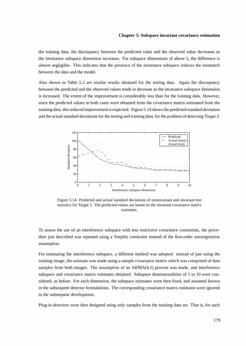
Chapter 5: Subspace invariant covariance estimation
the training data, the discrepancy between the predicted value and the observed value decreases as
the invariance subspace dimension increases. For subspace dimensions of above 5, the difference is
almost negligible. This indicates that the presence of the invariance subspace reduces the mismatch
between the data and the model.
Also shown in Table 5.2 are similar results obtained for the testing data. Again the discrepancy
between the predicted and the observed values tends to decrease as the invariance subspace dimension
is increased. The extent of the improvement is considerably less than for the training data. However,
since the predicted values in both cases were obtained from the covariance matrix estimated from the
training data, this reduced improvement is expected. Figure 5.14 shows the predicted standard deviation
and the actual standard deviations for the testing and training data, for the problem of detecting Target 3.
0 1 2 3 4 5 6 7 8 9 100
20
40
60
80
100
120
Interference subspace dimension
Stan
dard
dev
iatio
n
Predicted Actual (train)Actual (test)
Figure 5.14: Predicted and actual standard deviations of noninvariant and invariant teststatistics for Target 3. The predicted values are based on the invariant covariance matrix
estimates.
To assess the use of an interference subspace with less restrictive covariance constraints, the proce-
dure just described was repeated using a Toeplitz constraint instead of the first-order autoregressive
assumption.
For estimating the interference subspace, a different method was adopted: instead of just using the
training image, the estimate was made using a sample covariance matrix which was comprised of data
samples from both images. The assumption of an ARMA(4,1) process was made, and interference
subspace and covariance matrix estimates obtained. Subspace dimensionalities of 1 to 10 were con-
sidered, as before. For each dimension, the subspace estimates were then fixed, and assumed known
in the subsequent detector formulations. The corresponding covariance matrix estimates were ignored
in the subsequent development.
Plug-in detectors were then designed using only samples from the training data set. That is, for each
179

Section 5.8: Practical examples of invariant detectors
assumed interference subspace, an invariant covariance matrix estimate was made from data in this
set. This estimate was constrained to be Toeplitz. The final detector was then obtained by plugging
the resulting covariance matrix estimate into the subspace invariant detection statistic.
Table 5.3 shows the average target detectability figures as a function of the interference subspace
dimension. In this case the presence of the invariance subspace at no stage increases the detectability.
Invariance Training data Testing datadimension Targ1 Targ2 Targ3 Targ4 Targ5 Targ1 Targ2 Targ3 Targ4 Targ5
0 3.76 2.65 2.02 1.59 1.31 3.23 2.23 1.66 1.29 1.051 3.76 2.65 2.01 1.58 1.29 3.23 2.24 1.66 1.30 1.062 3.71 2.56 1.92 1.50 1.22 3.16 2.13 1.55 1.20 0.983 3.65 2.38 1.57 1.01 0.64 3.14 2.03 1.32 0.83 0.534 3.63 2.30 1.42 0.81 0.42 3.13 1.97 1.20 0.67 0.355 3.36 1.78 0.83 0.36 0.20 2.91 1.55 0.72 0.30 0.176 3.31 1.68 0.74 0.30 0.18 2.87 1.48 0.65 0.26 0.167 2.82 1.06 0.42 0.24 0.19 2.42 0.91 0.35 0.20 0.168 2.81 1.00 0.37 0.21 0.17 2.42 0.86 0.31 0.18 0.159 2.63 0.73 0.29 0.20 0.16 2.25 0.62 0.25 0.17 0.14
10 2.24 0.51 0.26 0.19 0.16 1.92 0.43 0.22 0.16 0.13
Table 5.3: Normalised separation between hypotheses for different invariance subspacedimensions and different targets.
The reason can be attributed to the high capacity of the general Toeplitz constrained model, and the
relative homogeneity of the data. That is, under a Toeplitz assumption the model is still flexible enough
to accurately model the data even when interference is apparently present. This may not be the case
for data which exhibit greater variability.
The test statistic also appears to generalise well, as can be determined from results when applied to
the testing data. The presence of the invariance subspace only reduces the detectability. The average
detectability in each case is smaller than that for the training data, as expected, but the difference is
quite small.
Table 5.4 shows actual standard deviations of the test statistics versus the standard deviations predicted
by the estimated model. Again the results are separated into training and testing data. For the training
data, the actual observed values are almost identical to the predicted values. This can again be attributed
to the relative freedom of the model under just a Toeplitz constraint. The model mismatch is therefore
almost identically zero in all cases, and the introduction of an invariance subspace then only serves to
reduce performance.
The presence of the interference subspace does reduce the mismatch between the predicted and the
observed test statistic variance for the test image. The difference is small, however, and hardly warrants
180
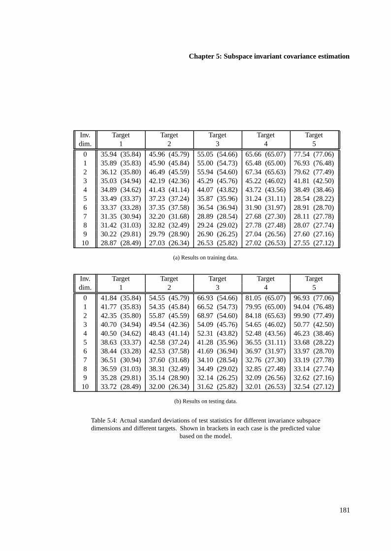
Chapter 5: Subspace invariant covariance estimation
Inv. Target Target Target Target Targetdim. 1 2 3 4 5
0 35.94 (35.84) 45.96 (45.79) 55.05 (54.66) 65.66 (65.07) 77.54 (77.06)1 35.89 (35.83) 45.90 (45.84) 55.00 (54.73) 65.48 (65.00) 76.93 (76.48)2 36.12 (35.80) 46.49 (45.59) 55.94 (54.60) 67.34 (65.63) 79.62 (77.49)3 35.03 (34.94) 42.19 (42.36) 45.29 (45.76) 45.22 (46.02) 41.81 (42.50)4 34.89 (34.62) 41.43 (41.14) 44.07 (43.82) 43.72 (43.56) 38.49 (38.46)5 33.49 (33.37) 37.23 (37.24) 35.87 (35.96) 31.24 (31.11) 28.54 (28.22)6 33.37 (33.28) 37.35 (37.58) 36.54 (36.94) 31.90 (31.97) 28.91 (28.70)7 31.35 (30.94) 32.20 (31.68) 28.89 (28.54) 27.68 (27.30) 28.11 (27.78)8 31.42 (31.03) 32.82 (32.49) 29.24 (29.02) 27.78 (27.48) 28.07 (27.74)9 30.22 (29.81) 29.79 (28.90) 26.90 (26.25) 27.04 (26.56) 27.60 (27.16)
10 28.87 (28.49) 27.03 (26.34) 26.53 (25.82) 27.02 (26.53) 27.55 (27.12)
(a) Results on training data.
Inv. Target Target Target Target Targetdim. 1 2 3 4 5
0 41.84 (35.84) 54.55 (45.79) 66.93 (54.66) 81.05 (65.07) 96.93 (77.06)1 41.77 (35.83) 54.35 (45.84) 66.52 (54.73) 79.95 (65.00) 94.04 (76.48)2 42.35 (35.80) 55.87 (45.59) 68.97 (54.60) 84.18 (65.63) 99.90 (77.49)3 40.70 (34.94) 49.54 (42.36) 54.09 (45.76) 54.65 (46.02) 50.77 (42.50)4 40.50 (34.62) 48.43 (41.14) 52.31 (43.82) 52.48 (43.56) 46.23 (38.46)5 38.63 (33.37) 42.58 (37.24) 41.28 (35.96) 36.55 (31.11) 33.68 (28.22)6 38.44 (33.28) 42.53 (37.58) 41.69 (36.94) 36.97 (31.97) 33.97 (28.70)7 36.51 (30.94) 37.60 (31.68) 34.10 (28.54) 32.76 (27.30) 33.19 (27.78)8 36.59 (31.03) 38.31 (32.49) 34.49 (29.02) 32.85 (27.48) 33.14 (27.74)9 35.28 (29.81) 35.14 (28.90) 32.14 (26.25) 32.09 (26.56) 32.62 (27.16)
10 33.72 (28.49) 32.00 (26.34) 31.62 (25.82) 32.01 (26.53) 32.54 (27.12)
(b) Results on testing data.
Table 5.4: Actual standard deviations of test statistics for different invariance subspacedimensions and different targets. Shown in brackets in each case is the predicted value
based on the model.
181
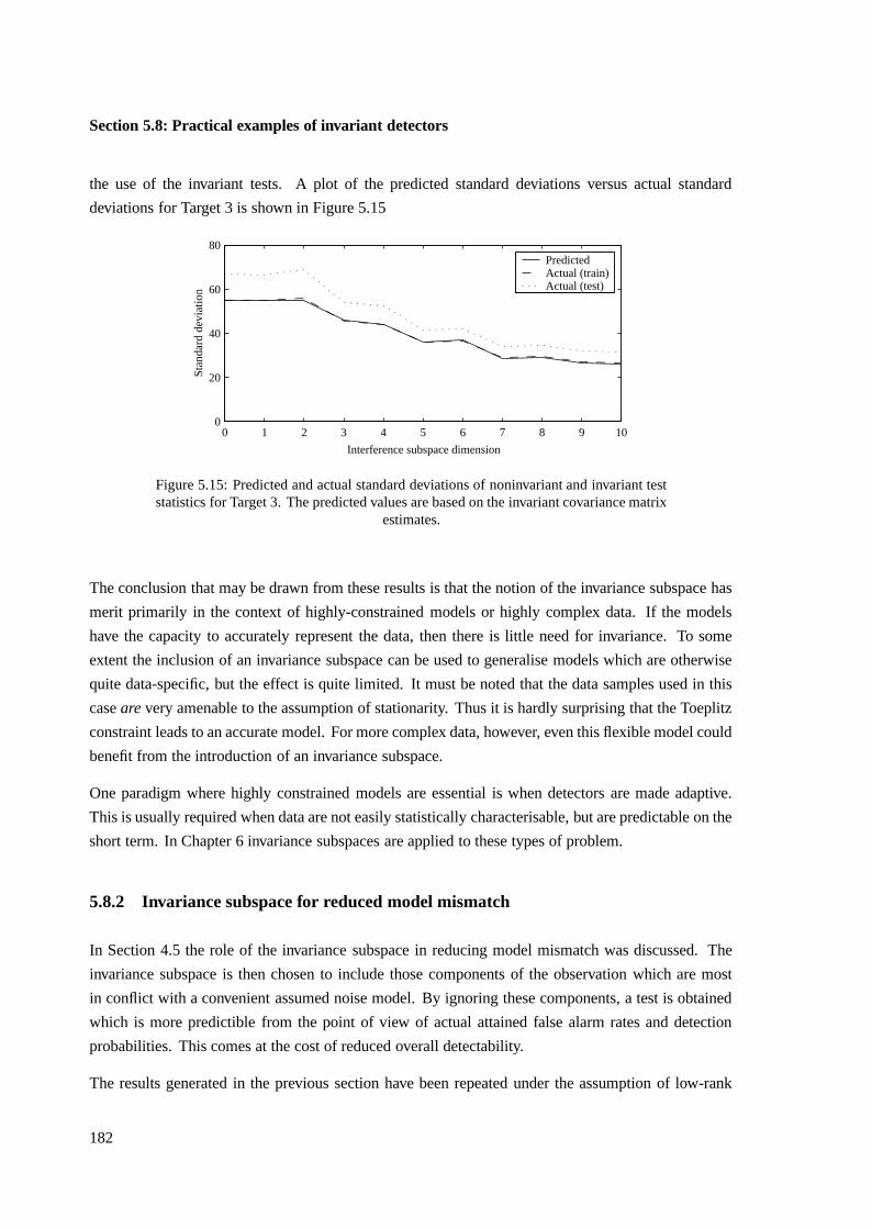
Section 5.8: Practical examples of invariant detectors
the use of the invariant tests. A plot of the predicted standard deviations versus actual standard
deviations for Target 3 is shown in Figure 5.15
0 1 2 3 4 5 6 7 8 9 100
20
40
60
80
Interference subspace dimension
Stan
dard
dev
iatio
n
Predicted Actual (train)Actual (test)
Figure 5.15: Predicted and actual standard deviations of noninvariant and invariant teststatistics for Target 3. The predicted values are based on the invariant covariance matrix
estimates.
The conclusion that may be drawn from these results is that the notion of the invariance subspace has
merit primarily in the context of highly-constrained models or highly complex data. If the models
have the capacity to accurately represent the data, then there is little need for invariance. To some
extent the inclusion of an invariance subspace can be used to generalise models which are otherwise
quite data-specific, but the effect is quite limited. It must be noted that the data samples used in this
case are very amenable to the assumption of stationarity. Thus it is hardly surprising that the Toeplitz
constraint leads to an accurate model. For more complex data, however, even this flexible model could
benefit from the introduction of an invariance subspace.
One paradigm where highly constrained models are essential is when detectors are made adaptive.
This is usually required when data are not easily statistically characterisable, but are predictable on the
short term. In Chapter 6 invariance subspaces are applied to these types of problem.
5.8.2 Invariance subspace for reduced model mismatch
In Section 4.5 the role of the invariance subspace in reducing model mismatch was discussed. The
invariance subspace is then chosen to include those components of the observation which are most
in conflict with a convenient assumed noise model. By ignoring these components, a test is obtained
which is more predictible from the point of view of actual attained false alarm rates and detection
probabilities. This comes at the cost of reduced overall detectability.
The results generated in the previous section have been repeated under the assumption of low-rank
182

Chapter 5: Subspace invariant covariance estimation
model mismatch, instead of a subspace interference. The invariance subspace is then estimated using
the method presented in Section 5.7, where simultaneous minimisation of the Frobenius norm over
the invariance subspace and the covariance matrix is performed. The results are very similar to those
using the assumption of subspace interference. They will therefore not be repeated here. It has been
observed that the invariance subspace estimates are quite similar in both cases, and the advantages of
including invariance are apparent for both formulations. This is a promising result, suggesting that
the precise details of the invariance formulation are not critical. It also raises the possibility that good
results may be obtained without the need for rigorous maximum likelihood procedures.
To explicitly demonstrate the concept of invariance subspace estimation for model mismatch, results
have therefore been generated for a different problem. In particular, the same test image used in
Section 4.5.2 and shown in Figure 4.11 was used, and invariant detectors designed for it. Again the
image was simply used to obtain noise samples, with no unknown target location problem implied.
The assumption was made that data samples extracted along horizontal lines in this image can be
treated as a realisation of the same stationary random process, at least in the subspace orthogonal to
the invariance subspace.
In anticipation of one of the primary topics of the next chapter, namely predictability in detection, the
data analysis was performed differently from the analysis in the previous section. In particular, the
following steps were performed:
• Initially the assumption of a first-order autoregressive process was made for the noise samples.
These samples were each of length 32, and obtained by extracting horizontal windows of data
from the image.
• A sample covariance matrix was calculated, using nonoverlapping data extracted from the entire
image. For the noninvariant detector, a simple constrained estimate of the covariance was
made. For the invariant detector, a three-dimensional invariance subspace was assumed. The
simultaneous estimation procedure which minimises the Frobenius distance between the relevant
covariance matrices, presented in Section 5.7, was used to obtain a covariance matrix estimate
and an invariance subspace estimate.
• Assuming accuracy all the estimates, a noninvariant and an invariant detector were developed
for two different targets. These targets were taken to be Target 2 and Target 3 from the previous
section. The estimate of the noise covariance matrix in each case was used to select the test
threshold, for 8 required false alarm rates (PFA).
• Each detector was then applied to a number of samples of data extracted from the image. Since
the samples contain only noise, the actual false alarm rate for each detector and each threshold
value could be found.
183

Section 5.8: Practical examples of invariant detectors
For both the noninvariant and invariant detectors, and for each of the two targets, the method described
was used to obtain plots of actual false alarm rates versus desired false alarm rates. If the models are
perfectly accurate for the data, then the difference between the actual and desired rates will be small.
Figure 5.16 shows the autocorrelation function and invariance subspace estimates obtained using this
method. These estimates do not depend on the targets to be detected. It may be observed that the
0 5 10 15 20 25 300
5
10
15
20
25
30
Lag
Cov
aria
nce
prod
uct
(a) Autocorrelation function estimate.
0 5 10 15 20 25 30−0.4
−0.2
0
0.2
0.4
Lag
Cov
aria
nce
prod
uct
(b) Basis functions of three-dimensional invariance subspace estimate.
Figure 5.16: Invariant autocorrelation function and invariance subspace basis estimatesunder first-order autoregressive assumption.
dotted basis function in Figure 5.16(b) quite closely resembles target 3. It may be expected that the
detectability for the invariant test will suffer for this target.
Figure 5.17 shows results for the subspace invariant detectors using the autocorrelation function and
invariance subspace estimates shown in Figure 5.16. The first plot corresponds to the predictability of
184

Chapter 5: Subspace invariant covariance estimation
0.05 0.1 0.15 0.2 0.25 0.3 0.35 0.40
0.1
0.2
0.3
0.4
Required PFA
Obs
erve
d P FA
Ideal No invariance With invariance
(a) Target 2.
0.05 0.1 0.15 0.2 0.25 0.3 0.35 0.40
0.1
0.2
0.3
0.4
Required PFA
Obs
erve
d P FA
Ideal No invariance With invariance
(b) Target 3.
Figure 5.17: Actual false alarm rates versus ideal rates for noninvariant and invariantdetection using AR(1) model. A 3-D invariance subspace was assumed.
the test for Target 2, and the second for Target 3. Also shown are results for the noninvariant detectors,
which at no time use data in the invariance subspace in their calculation. It is clear that the invariant
detector produces a test that exhibits performance closer to the design conditions. In particular, for
Target 2, the invariance subspace has improved the modelling considerably. The improvement for
Target 3 is smaller, but still significant.
What is not demonstrated in these plots is that the overall detectability has decreased with the in-
troduction of the invariance subspace: the ratio of the normalised separation between the invariant
and noninvariant test is about 0.7 for Target 2, and 0.45 for Target 3. There is therefore a significant
reduction in detectability associated with the inclusion of the invariance subspace.
185
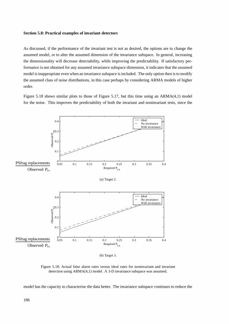
Section 5.8: Practical examples of invariant detectors
As discussed, if the performance of the invariant test is not as desired, the options are to change the
assumed model, or to alter the assumed dimension of the invariance subspace. In general, increasing
the dimensionality will decrease detectability, while improving the predictability. If satisfactory per-
formance is not obtained for any assumed invariance subspace dimension, it indicates that the assumed
model is inappropriate even when an invariance subspace is included. The only option then is to modify
the assumed class of noise distributions, in this case perhaps by considering ARMA models of higher
order.
Figure 5.18 shows similar plots to those of Figure 5.17, but this time using an ARMA(4,1) model
for the noise. This improves the predictability of both the invariant and noninvariant tests, since the
0.05 0.1 0.15 0.2 0.25 0.3 0.35 0.40
0.1
0.2
0.3
0.4
Required PFA
Obs
erve
d P FA
Ideal No invariance With invariance
PSfrag replacements
Observed PFA
(a) Target 2.
0.05 0.1 0.15 0.2 0.25 0.3 0.35 0.40
0.1
0.2
0.3
0.4
Required PFA
Obs
erve
d P FA
Ideal No invariance With invariance
PSfrag replacements
Observed PFA
(b) Target 3.
Figure 5.18: Actual false alarm rates versus ideal rates for noninvariant and invariantdetection using ARMA(4,1) model. A 3-D invariance subspace was assumed.
model has the capacity to characterise the data better. The invariance subspace continues to reduce the
186

Chapter 5: Subspace invariant covariance estimation
mismatch, however. With the better modelling the detectability for the invariant detectors improves
in both cases, with the ratio of the normalised separation increasing to 0.79 and 0.51, for Target 2 and
Target 3 respectively.
It may be noted that, even with the invariance subspace, the predictability of the test statistic for Target 3
is fairly low. This may be attributed directly to the fact that the target lies substantially in the invariance
subspace. The target therefore resembles components of the noise which are difficult to characterise
effectively. Any detector will suffer under these conditions.
Predictability in detection is especially important when detectors are made adaptive. For these detectors
to be effective, however, constraints are essential to improve the parameter estimation. If the constrained
models are too restrictive, an invariance subspace can be introduced. This subspace can improve the
validity of the constrained models, thereby improving overall performance. This topic is addressed in
the next chapter.
187

Section 5.8: Practical examples of invariant detectors
188

Chapter 6
Adaptive detection with invariance
In this chapter the role of subspace invariant detectors in adaptive detection is presented. Two cases
are considered in detail, namely where secondary noise-only observations are available for estimation,
and where simultaneous estimation and detection has to be performed on the same data sample. In this
latter case constraints on the set of allowed noise densities are essential.
As discussed in the literature review chapter, in an adaptive context with secondary observations
available, the work by Burgess and Van Veen [20] is of considerable interest. They propose subspace
projections as a general method of dimensionality reduction when covariance matrices are completely
unknown. That is, by reducing the dimensionality, the ratio of the amount of data available for
estimation to the number of noise parameters is improved. The subspace projections can therefore lead
to better performance even though data are discarded.
Because covariance constraints are used in the majority of this thesis, the subspace projection method
for dimensionality reduction is not appropriate. Instead, the data-to-parameter ratio is improved by
limiting the set of possible values for the unknown parameters. Thus in this work certain dimensions of
the observation space are ignored for a different reason: because they do not conform to the modelling
assumptions.
The chapter begins with a decomposition of the detection problem into disjoint subspaces. This is
useful for demonstrating the way in which the different components of an observation contribute to the
overall detection statistic. In particular, for the known noise parameter case, it is shown that the noise-
only components serve only to reduce the variance in the conditional distribution of the target-carrying
components. When unknown noise parameters are included, a separate mechanism arises by which
the noise-only subspace can improve detection: the observed data in this subspace contain additional
information regarding the distribution of the noise in the target subspace. Thus further improvements
may be obtained from using the noise-only component.
189
Section 6.1: Subspace decomposition of the detection problem
Section 6.2 discusses in detail the problem of adaptive detection when secondary noise-only observa-
tions are available which share the distribution of the primary data. Two tests are considered, namely
the AMF and the GLRT discussed in previous chapters. It is argued that the formulations of these tests
presented in the literature are inappropriate in some instances, and modified derivations are presented
which more accurately represent common problems. The resulting tests are shown to have a CFAR
property in the case where there are no constraints on the covariance matrix estimate. In both these
cases it is demonstrated that the inclusion of an invariance subspace for improving modelling is trivial,
and the tests continue to be CFAR. Finally, a simplified AMF formulation is presented which has some
computational savings.
Section 6.3 discusses issues relating to covariance constraints in the testing problem. When constrained
estimates are used the tests presented no longer have a CFAR property, but they are nevertheless
asymptotically CFAR whenever the noise estimates are consistent. The tests are then applied to the
problem of simultaneous estimation and detection from a single sample of data, where covariance
constraints are essential. It is shown that the AMF and GLRT formulations can be used for this
problem. The use of estimates which are invariant to possible target presence are also proposed in
these instances. These estimates overcome certain difficulties which otherwise arise.
In Section 6.4 results are presented showing the use of invariance subspaces in the detectors discussed.
In all cases it is assumed that there is only a single sample of data available for the training and
testing. It is demonstrated that the invariance subspace can result in a detector which is considerably
more predictable than the corresponding noninvariant detector. It also overcomes the need for a
preprocessing stage to make the data better suit the model.
6.1 Subspace decomposition of the detection problem
In time-series analysis, it is commonly required to predict the value of a future sample based on
previously observed samples. This prediction is achieved through the use of a statistical model for the
process. In the event that the process generating the samples is MVN and the model parameters are
known, a linear predictor formulation is appropriate. If all assumptions are valid, then the predicted
value minimises the expected mean square error between itself and the actual value obtained [113].
A similar interpretation may be applied to the general problem of predicting one set of components of
a MVN observation from a different set of components. In particular, it is possible to reformulate the
optimal detector in coloured noise into an estimation stage, followed by detection. The estimation stage
makes use of the data components in the noise-only subspace to predict the nominal value of the noise
component in the target-carrying subspace. The difference between the observed data in the target
subspace and this predicted value then constitutes a sufficient statistic for the optimal detection. The
interpretation may also be extended to the invariant detector discussed in Chapter 4, by appropriately
190
Chapter 6: Adaptive detection with invariance
ignoring the invariance subspace in the prediction.
6.1.1 Two-stage decomposition of the detection problem
The development is as follows: suppose the observation space is decomposed into three mutually
disjoint subspaces 〈UI 〉, 〈UT 〉, and 〈UN 〉, which are p, t , and (n − p − t)-dimensional respectively.
These spaces are spanned by the matrices U I , UT , and UN , each with orthonormal columns. U I is
chosen to span the invariance subspace, which is ignored in the detection. 〈UT 〉 is the projection of
the target-carrying subspace out of the invariance subspace — in other words, all targets that may be
present lie in 〈(UI UT )〉, with UI ⊥ UT . 〈UN 〉 is then the remaining subspace after 〈UT 〉 and 〈UI 〉have been removed. It is a noise-only subspace, containing data with the same distribution under each
possible hypothesis.
Suppose that it is required to detect any instance of the parametric target sθ in additive noise n : N [0, C].By expanding on the alternative basis, the observed data x may be represented by the components
xt = UTT x, xi = UT
I x, and xn = UTN x. Useful interpretations may be applied to these components:
• xt is the potential target-carrying portion of the observation, which is not affected by the invari-
ance subspace. It is also subject to noise.
• xi is the component to which the test is required to be invariant, and should therefore be ignored
in any subsequent development.
• xn is the component of the observation that is completely unaffected by target presence, and
contains only valid noise data. It therefore only provides information regarding the additive
noise in the observation.
The reformulation of the detection problem is obtained by means of the following interpretation: since
target presence only affects the component xt in a useful manner, it should be possible to perform the
entire detection process in the subspace 〈UT 〉. However, since the noise-only component xn contains
information regarding the noise in this target subspace, it is still useful from the point of view of
detection. The approach is therefore to use the data xn to predict the value of the noise in the target
subspace. It is then shown that the difference between the actual observed data in this subspace and
the predicted value is sufficient for the detection. Thus it may be concluded that the only role of the
noise-only subspace (at least for the case of a known noise distribution) is to provide information
regarding the data in the target subspace.
The assertions made in the previous paragraph may be proved using the Gauss-Markov theorem and
some inversion formulae for partitioned matrices. Firstly, with xt and xn as defined, and with x :
191

Section 6.1: Subspace decomposition of the detection problem
N [0, C], under H0 (xt
xn
): N
[(0
0
),
(UT
T CUT UTT CUN
UTN CUT UT
N CUN
)]. (6.1)
Similarly, under H1, (xt
xn
): N
[(UT
T sθ
0
),
(UT
T CUT UTT CUN
UTN CUT UT
N CUN
)]. (6.2)
The target parameter θ is assumed known for purposes of the detection problem.
As described, the noise-only subspace is used to predict the value of the noise component in the
subspace 〈UT 〉. Under the MVN assumption, the natural estimate for this purpose is the conditional
expectation E{xt |xn}. By applying the Gauss-Markov theorem, the appropriate conditional distribution
is given by
xt |xn : N [UTT CUN (UT
N CUN )−1xn, Q], (6.3)
where Q = UTT CUT − UT
T CUN (UTN CUN )−1UT
N CUT . Note that this distribution applies under H0,
since it is assumed to describe only the noise component of the observation x = sθ + n. It is now
shown that with xt = E{xt |xn}, the statistic xt − xt is sufficient for the invariant detection problem,
where invariance is required to data components in the subspace 〈U I 〉.
The distribution of the statistic xt − xt is N [0, Q] under H0, and N [UTT sθ , Q] under H1. For known θ ,
the optimal test statistic of H0 versus H1 given the data xt − xt is therefore
t = sTθ UT Q−1(xt − xt)
= sTθ UT Q−1(xt − UT
T CUN (UTN CUN )−1xn. (6.4)
A fairly lengthy simplification process now follows. Noting that the conditional covariance matrix Q
can be written as
Q = UTT
[C − CUN (UT
N CUN )−1UTN C]
UT , (6.5)
Equation 4.28 can be used to show that
Q = UTT
(
UT UI
)((UTT
UTI
)C−1
(UT UI
))−1 (UT
T
UTI
)UT . (6.6)
Note that Equation 4.28 requires orthogonality between UH and UI to hold, which is why UH in that
expression is taken to be (UT UI ) when applied here. This last expression for Q may be simplified to
Q =(
It×t 0)(UT
T C−1UT UTT C−1UI
UTI C−1UT UT
I C−1UI
)−1 (It×t
0
). (6.7)
192
Chapter 6: Adaptive detection with invariance
Therefore, Q is simply the top left t × t elements of the inverse of the block matrix
A =(
UTT C−1UT UT
T C−1UI
UTI C−1UT UT
I C−1UI
). (6.8)
The partitioned matrix inversion formula [6, p. 179] may then be used to derive a final useful form for
the conditional covariance:
Q−1 = UTT C−1UT − UT
T C−1UI (UTI C−1UI )
−1UTI C−1UT . (6.9)
The second portion of the simplification relates to the quantity xt − xt . In this case, noting that
xt − xt = UTT x − UT
T CUN (UTN CUN )−1UT
N x
= UTT [C − UT
T CUN (UTN CUN )−1UT
N C]C−1x, (6.10)
the same results as before may be used to show that
xt − xt =(
It×t 0)(UT
T C−1UT UTT C−1UI
UTI C−1UT UT
I C−1UI
)−1 (UT
T C−1x
UTI C−1x
). (6.11)
Once again the partitioned matrix inversion formula may be used (in conjunction with the result
obtained in Equation 6.9) to show that
xt − xt =(
Q −QUTT C−1UI (UT
I C−1UI )−1)(UT
T C−1x
UTI C−1x
), (6.12)
so that
xt − xt = QUTT C−1x − QUT
T C−1UI (UTI C−1UI )
−1UTI C−1x. (6.13)
Finally, substituting this result into the test statistic in Equation 6.4 yields the following expression:
t = sTθ UT UT
T C−1x − sTθ UT UT
T C−1UI (UTI C−1UI )
−1UTI C−1x. (6.14)
Again using the relationship in Equation 4.28 can be written as
t = sTθ UT UT
T UH(UTH CUH)−1UT
H x, (6.15)
where UH is a matrix spanning the subspace complementary to 〈U I 〉. Now UT UTT sθ is the orthogonal
projection of sθ into the space 〈UT 〉, which is contained in the space 〈UH 〉. Thus UT UTT sθ = UH UT
H sθ ,
and
t = sTθ UH(UT
H CUH)−1UTH x. (6.16)
193
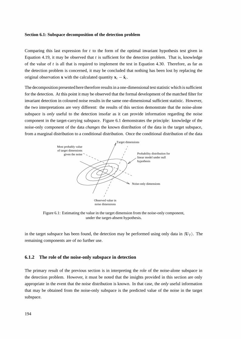
Section 6.1: Subspace decomposition of the detection problem
Comparing this last expression for t to the form of the optimal invariant hypothesis test given in
Equation 4.19, it may be observed that t is sufficient for the detection problem. That is, knowledge
of the value of t is all that is required to implement the test in Equation 4.30. Therefore, as far as
the detection problem is concerned, it may be concluded that nothing has been lost by replacing the
original observation x with the calculated quantity xt − xt .
The decomposition presented here therefore results in a one-dimensional test statistic which is sufficient
for the detection. At this point it may be observed that the formal development of the matched filter for
invariant detection in coloured noise results in the same one-dimensional sufficient statistic. However,
the two interpretations are very different: the results of this section demonstrate that the noise-alone
subspace is only useful to the detection insofar as it can provide information regarding the noise
component in the target-carrying subspace. Figure 6.1 demonstrates the principle: knowledge of the
noise-only component of the data changes the known distribution of the data in the target subspace,
from a marginal distribution to a conditional distribution. Once the conditional distribution of the data
Probability distribution forlinear model under nullhypothesis
Observed value innoise dimensions
Most probably value
given the noiseof target dimensions
Noise-only dimensions
Target dimensions
Figure 6.1: Estimating the value in the target dimension from the noise-only component,under the target-absent hypothesis.
in the target subspace has been found, the detection may be performed using only data in 〈UT 〉. The
remaining components are of no further use.
6.1.2 The role of the noise-only subspace in detection
The primary result of the previous section is in interpreting the role of the noise-alone subspace in
the detection problem. However, it must be noted that the insights provided in this section are only
appropriate in the event that the noise distribution is known. In that case, the only useful information
that may be obtained from the noise-only subspace is the predicted value of the noise in the target
subspace.
194
Chapter 6: Adaptive detection with invariance
The decomposition presented also provides a reasonable solution to the problem of assessing whether
an assumed noise model is appropriate for detecting a known target, given a sample of actual noise data.
In general, it is difficult to ascertain whether model mismatch or inaccuracy will have a detrimental
effect on detector performance: it is quite conceivable that a partially-incorrect model is still accurate
for detection. However, the subspace decomposition presented can provide a means of obtaining such
information: if the best predicted value of the noise in the target-carrying subspace is similar to the
value that is actually observed under the null hypothesis, then model accuracy for detection is indicated.
Note that this validation process has the advantage that it specifically takes the target subspace into
account.
The results presented suggest that the use of the noise-alone subspace is only useful insofar as observing
xn reduces the uncertainty of the data in the target-carrying subspace. Although true when the noise
distribution is assumed known, if the noise contains unknown parameters this statement is no longer
true. When unknown parameters are included in the formulation, the noise-only subspace also provides
information regarding the values of these parameters. This provides further information regarding the
distribution of the data in the target subspace, in addition to the actual noise component in this subspace.
To explain these results in more detail, suppose that the nominal noise distribution is N [0, C(θ )]. In
that case, (xt
xn
): N
[(0
0
),
(Ct t(θ) Ctn(θ)
Cnt(θ) Cnn(θ)
)]. (6.17)
Suppose for now that θ is fixed and known. The noise covariance matrix is then known, and the
results presented previously apply. That is, the component xn can be used to make an estimate of the
noise component in xt , which is useful in the subsequent detection. This, however, is only possible
when Ctn(θ) and Cnt(θ) are nonzero — in the event that the coupling between the subspaces is
zero, knowledge regarding the component of the data in the subspace 〈UN 〉 provides no information
regarding the noise in 〈UT 〉. In that case, observing xn contributes nothing to the final detector, which
may effectively be performed entirely in the subspace 〈UT 〉. The subspaces are effectively independent.
When θ is unknown, this last conclusion no longer applies. Then, even if C tn(θ) and Cnt(θ) are zero
for all values of θ , the data in the noise-only subspace still contain information that is useful to the
decision process in the subspace 〈UT 〉. This is because the distribution of xn depends on θ . Thus, by
observing xn , information is obtained regarding the details of the distribution of the data component
xt .
6.2 Adaptive detection with secondary noise-only observations
Section 5.1 presented an outline of solutions to the problem of detecting a known target in the presence of
partially-known noise, when an invariance subspace is included in the formulation. It was demonstrated
195
Section 6.2: Adaptive detection with secondary noise-only observations
that the resulting tests require subspace invariant estimates of the noise parameters.
The case of completely known targets does not generally lead to tests which exhibit a constant false
alarm rate. For example, Reed, Mallet and Brennan [111] discuss a plug-in formulation for this known
target detection problem when the covariance matrix is completely unspecified, and the distribution
of the test statistic under H0 depends on the unknown covariance. This makes it difficult to select a
test threshold meaningfully, since the properties of the test will in general depend on the unknown
parameter values.
In [116], Robey et al. demonstrate that the plug-in principle, when applied to the problem of detecting
the presence of the target αs for unknown α, leads to a CFAR test. That is, the introduction of
the parameter α results in the test having a normalisation component which improves its statistical
properties under the noise-only hypothesis. They call this test the adaptive matched filter (AMF).
Similarly, Kelly [80] shows that the introduction of an unknown target scaling parameter results in the
GLRT for the same problem having a CFAR property.
Both the AMF test and the GLRT in these cases assume the presence of secondary target-free observa-
tions, which share the distribution of the noise component of the data to be tested for target presence.
The observations are all assumed to be mutually independent and zero mean, and the only unknown pa-
rameter in their distribution is the covariance matrix. No constraints are placed on the set of allowable
covariances.
The tests presented by Robey et al. and Kelly both deal with the problem of complex signals and
targets. The unknown target scaling parameter α is also complex, and is permitted to take on any
value whatsoever. For real observations, this formulation is inappropriate for many problems: since
the parameter α is unconstrained, it can take on both positive and negative values. Thus the tests
will produce the same result when presented with the data observation x as they will when presented
with −x. They will therefore detect instances of both the target αs and the target −αs, without
discrimination.
When a noise model is used to represent an environment comprised substantially of clutter, this two-
sided property of the tests is highly undesirable if only positive scale coefficients are relevant. In x-ray
images, for example, tumours always exhibit greater attenuation than surrounding tissue. It makes no
sense then to allow false alarms based on regions which resemble tumours in shape, but have inverted
attenuation profiles. Thus it is desirable to reformulate the AMF and GLRT to better represent this
class of problems.
In the two sections which follow, the AMF and GLRT are modified for the problem of one-sided
hypothesis testing, where the target coefficient is still considered unknown, but is constrained to be
nonnegative. It is demonstrated that the resulting tests are once again CFAR. Initially the inclusion of
an invariance subspace is not considered: this case is discussed in Section 6.2.3. Also, constraints on
196
Chapter 6: Adaptive detection with invariance
the allowed covariance matrix are not considered, but are presented in Section 6.3. In Section 6.2.4
a simplified AMF formulation is presented which is less adaptive, but avoids the need for a matrix
inversion in its calculation.
6.2.1 AMF reformulated for positive target coefficients
The derivation in this section is similar to that presented in [116], with the exception that the target
amplitude parameter is required to be nonnegative. Thus it is required to detect the target αs in coloured
noise, with α > 0. With x the data to be tested for target presence, the null hypothesis is x : N [0, C].The composite alternative is that x : N [αs, C], for some α > 0.
In practice, the covariance matrix C is unknown, and is estimated from the secondary noise-only
observations x1, . . . , xM . However, for purposes of the AMF test development, it is assumed that C is
known, and the GLRT is derived for detecting the presence of the target x under these conditions. The
GLRT statistic for this known covariance matrix problem is
tGLRT(x) = lnmaxα≥0(2π)−n/2|C|−1/2e−1/2(x−αs)T C−1(x−αs)
(2π)−n/2|C|−1/2e−1/2xT C−1x
= maxα≥0
{αsT C−1x − 1/2α2sT C−1s
}. (6.18)
It is easy to show that the value α of α that maximises the previous expression is given by
α =
sT C−1xsT C−1s sT C−1x ≥ 0
0 sT C−1x < 0,(6.19)
which assumes the constraint α > 0. Substituting back into 6.18, the GLRT statistic becomes
tGLRT(x) =
12
(sT C−1x)2
sT C−1s sT C−1x ≥ 0
0 sT C−1x < 0.(6.20)
The resulting test is to compare this to a threshold and decide H1 if exceeded.
If only positive values of the threshold are permitted, then the test tGLRT(x)H1><H0
η′ can be cast into the
simplified formsT C−1x√sT C−1s
H1><H0
η. (6.21)
This follows since H1 is never decided if sT C−1x < 0. To form the final AMF test statistic, the estimate
C of C obtained from the secondary data vectors is substituted into this expression. Thus as long as
197

Section 6.2: Adaptive detection with secondary noise-only observations
the threshold η is always chosen to be positive, the AMF is
tAMF(x) = sT C−1x√sT C−1s
H1><H0
η. (6.22)
Note that the square of this test statistic is precisely the test developed by Robey et al. for the
corresponding two-sided problem.
Using the same methods presented in [116], it can be demonstrated that the distribution of the test
statistic tAMF(x) is independent of the actual noise covariance C. Firstly, consider the term sT C−1x in
the numerator. Under the null hypothesis, x : N [0, C] and M C : W [C; n, M], where W [C; n, M]denotes an n-dimensional Wishart distribution with M degrees of freedom, and matrix scale parameter
C [30, p. 302]. It is assumed that C has been obtained using M additional independent observations.
Now
sT C−1x = sT C−1/2C1/2C−1C1/2C−1/2x = uT C−1y, (6.23)
where u = C−1/2s, y = C−1/2x, and C = C−1/2CC−1/2. The transformed vector y has a N [0, I]distribution. Also, from the properties of the Wishart distribution [30, p. 302], the distribution of M C
is W [I; n, M]. The distribution of both of these quantities is therefore independent of the unknown
covariance C. The only term in this alternative form of the numerator which depends on C is the vector
u.
It can be shown that this term depends on C only through a scalar coefficient d . Let U be a unitary
transformation chosen such that
d e1 = UT u, (6.24)
with e1 the first unit vector (1 0 · · · 0)T . Then
uT C−1y = uT UUT C−1UUT y = d eT1 G−1z, (6.25)
where now G = UT CU and z = UT y. Since the distribution of z : N [0, I] and MG : W [I; n, M], it
is evident that the unknown covariance matrix C enters the distribution of sT C−1x only through d .
Using a similar analysis on the denominator term sT C−1s,
sT C−1s = sT C−1/2C1/2C−1C1/2C−1/2s = uT C−1u
= uT UUT C−1UUT u = d2eT1 G−1e1, (6.26)
where once again the distribution of MG is W [I; n, M]. Thus the distribution of the denominator also
only depends on C through the value of d .
198

Chapter 6: Adaptive detection with invariance
Returning to the AMF, the test statistic can therefore be written as
tAMF = d eT1 G−1z√
d2eT1 G−1e1
= eT1 M−1z√eT
1 G−1e1
. (6.27)
Since d can be eliminated from the statistic, the remaining quantity in no way depends on C. Thus
under H0 the distribution of the test statistic is completely determined, and does not depend on the
underlying covariance parameters. A fixed test threshold can therefore be used to yield a desired false
alarm rate.
In practice, the restriction that the threshold be positive means that this result only holds for tests of
sufficiently small size. Since the distribution under H0 is symmetric about the origin, the test presented
is applicable whenever the required false alarm rate is less than 0.5. In most cases this is hardly a
restriction, unless high detection rates are required at the cost of a large number of false alarms.
It is easy to see how this modified formulation, which permits only positive target coefficients, can
improve detection performance. As mentioned, the AMF test statistic presented in the literature makes
use of the square of the statistic obtained here. Thus, when compared to a threshold, the unconstrained
test makes a decision of target presence whenever the quantity tAMF above is either greater than or
smaller than a set threshold. The modified formulation for positive target coefficients, however, only
decides H1 when the value of tAMF is greater than a threshold. Thus for the same threshold value, the
two tests have the same detection probability, but the false alarm rate in the latter case is halved. This
translates directly to better detection.
No attempt has been made to develop a closed-form solution for the density of this test statistic under
either hypothesis. However, the limiting distribution as the number of secondary data vectors increases
can be found, and is useful for subsequent developments. Suppose that the distribution of the secondary
vectors and of x under H0 is N [0, C] under H0. Since the sample covariance matrix is a consistent
estimator of the actual covariance, as M increases, C tends towards C. The variance in this estimate
also goes to zero. Thus the AMF test statistic
sT C−1x√sT C−1s
−→ sT C−1x√sT C−1s
, as M −→ ∞. (6.28)
With x : N [0, C], this quantity has a N [0, 1] distribution under H0.
Through a similar set of arguments it can be seen that this test is also asymptotically optimal for
detecting the target αs in noise, for any α > 0. It approaches the optimal matched filter for the known
covariance matrix case.
Thus it has been shown that the AMF of Robey et al. can be reformulated to detect only instances
of targets which have a positive coefficient. In the next section it is shown that Kelly’s GLRT can be
199
Section 6.2: Adaptive detection with secondary noise-only observations
similarly modified, again resulting in a CFAR test.
A final point to note with regard to this test, and those which follow, is that when written in the form
sT C−1xH1><H0
√sT C−1s, (6.29)
an adaptive thresholding interpretation is appropriate. Thus the value of the test component sT C−1x
may be calculated and compared to the threshold value√
sT C−1s, which is itself a function of the
estimated noise characteristics. The same test is achieved using this interpretation.
6.2.2 GLRT reformulated for positive target coefficients
As in the previous section, it is assumed that it is required to detect the presence of some positive
scaling of the target s in zero-mean noise with an unknown and unconstrained covariance matrix. The
data to be tested for target presence are x, and it is assumed that M additional noise-only observations
are available for estimation. (Note that this is in contrast to the multiple observation GLRT formulation
in Section 5.1.2, where the primary data vector was taken to be x1.) Thus the null hypothesis is that
x, x1, . . . , xM : N [0, C], and the alternative is that x : N [αs, C] for some α > 0, with x1, x2, . . . , xM :N [0, C]. The covariance matrix C is completely unknown.
The derivation of the test proceeds in the same way as in [80], up to the point where it is necessary to
maximise the likelihood ratio over the unknown factor α. That is, the GLRT statistic is given by
tGLRT(x, x1, . . . , xM) = maxα,C(2π)−(M+1)n/2|C|−(M+1)/2e−1/2(x−αs)T C−1(x−αs)−1/2∑M
i=1 xTi C−1xi
maxα,C(2π)−(M+1)n/2|C|−(M+1)/2e−1/2xT C−1x−1/2∑M
i=1 xTi C−1xi
.
(6.30)
Using standard results of MLEs of unknown covariance matrices, it is easy to show that the numerator
is maximised over C by the choice C1 = ((x − αs)(x − αs)T + MC)/(M + 1), where
C = 1
M
M∑
i=1
xi xTi . (6.31)
Similarly, the denominator takes on a maximum for C0 = (xxT + MC)/(M + 1). Substituting these
values into the test statistic and simplifying yields the result
tGLRT(x, x1, . . . , xM) = maxα≥0 |C1|−(M+1)/2
|C0|−(M+1)/2= maxα≥0 |(x − αs)(x − αs)T + MC|−(M+1)/2
|xxT + MC|−(M+1)/2.
(6.32)
Without changing the test, the monotonically increasing transformation t −→ t 2/(M+1) can be made,
200
Chapter 6: Adaptive detection with invariance
resulting in the modified test statistic
tGLRT = |xxT + MC|minα≥0 |(x − αs)(x − αs)T + MC|
. (6.33)
Using the same identities presented by Kelly, namely that |zzT + S| = |S|(1 + zT S−1z), this statistic
can be written as
tGLRT = (1 + 1/MxT C−1x)
minα≥0(1 + 1/M(x − αs)T C−1(x − αs)). (6.34)
At this point the minimisation over α can be performed.
As for the case of the AMF, the constrained minimum of the denominator over α ≥ 0 occurs for
α =
sT C−1xsT C−1s
sT C−1x ≥ 0
0 sT C−1x < 0.(6.35)
The resulting likelihood ratio test statistic is therefore
tGLRT =
1+1/MxT C−1x
1+1/MxT C−1x−1/M (sT C−1x)2
sT C−1s
sT C−1x ≥ 0
1 sT C−1x < 0
=
11−γ
sT C−1x ≥ 0
1 sT C−1x < 0,(6.36)
with
γ = (sT C−1x)2
(sT C−1s)(M + xT C−1x). (6.37)
Now, using the Cauchy-Schwarz inequality with the inner product 〈u, v〉 = uT C−1v [4, p. 227], it can
be seen that
(sT C−1x)2 ≤ (sT C−1s)(xT C−1x) < (sT C−1s)(M + xT C−1x), (6.38)
where the additional result has been used that C is nonsingular and positive definite. Thus it must
always be the case that 0 ≤ γ < 1. On this interval tGLRT ≥ 1, and the monotonically increasing
transformation t −→ M(1 − 1/t) can be applied to the value of the test statistic. For testing purposes,
this yields the equivalent statistic
tGLRT =
M(sT C−1x)2
(sT C−1s)(M+xT C−1x)sT C−1x ≥ 0
0 sT C−1x < 0.(6.39)
The GLRT compares this value to a threshold, and decides H1 when exceeded.
Once again for sufficiently large threshold values this statistic can be modified, by taking square roots,
201
Section 6.2: Adaptive detection with secondary noise-only observations
to produce the test
tGLRT = sT C−1x√
sT C−1s√
1 + 1/MxT C−1x
H1><H0
η. (6.40)
For this to hold requires that η > 0, which in account of the symmetry of the distribution corresponds
to a false alarm rate of less than 0.5. Thus as long as the required size is smaller than 0.5, the above
test represents the GLRT for the problem.
The distribution of this test statistic under H0 is independent of the unknown parameters. From the
discussion of the AMF, it is apparent that the distribution of the ratio sT C−1x/√
sT C−1s is independent
of both α and C. Additionally, the term xT C−1x can be shown to have a distribution independent of C
under H0:
xT C−1x = xT C−1/2C1/2C−1C1/2C−1/2x = yT C−1y, (6.41)
with y : N [0, I] and MC : W [I; n, M] as before. Thus the density of the term√
1 + 1/MxT C−1x does
not depend on the unknown covariance C, and the distribution of the test statistic tGLRT in Equation 6.40
is similarly independent.
Kelly [80] provides analytical solutions for the distribution of the test statistic, its size, and its power, for
the case where the target amplitude parameter is unconstrained. The functions are complex, however,
and provide little insight. Thus no attempt has been made to calculate these quantities for the modified
test presented here. What can quite simply be observed, however, is the limiting distribution of the
test statistic when large numbers of secondary noise-only observations are available. For large M ,√1 + 1/MxT C−1x ≈ 1 and C ≈ C. Thus the test statistic is approximately
tGLRT ≈ sT C−1x√sT C−1s
. (6.42)
Under H0, x : N [0, C], so the limiting distribution of tGLRT is also N [0, 1].
6.2.3 Subspace invariant AMF and GLRT formulations
When secondary noise-only observations are available, and it is required to detect a known target in
noise with unknown covariance, the presence of an invariance subspace causes no complications if
the covariance is unconstrained. That is, for observed secondary observations x1, . . . , xM and primary
data x, the invariant detection problem can simply be formulated in terms of the projected components
y1, . . . , yM and y, with yi = UTH xi and y = UT
H x. The presence of the target in the vector y will be of
the form αUTH s, if it appeared in the original as αs.
The subspace invariant detection problem can therefore be reformulated as follows: test for the presence
of the target αUTH s in the observation y, where y1, . . . , yM are secondary noise-only data, assumed to
202
Chapter 6: Adaptive detection with invariance
be zero mean, with completely unknown covariance.
An advantage of the invariance subspace formulation is that the distributions of the secondary data no
longer have to be considered equal: only the marginal distributions in the subspace orthogonal to the
invariance subspace must be the same. This can extend the applicability of the tests to situations where
they could otherwise not be applied.
The AMF presented in the previous section can therefore be trivially applied. Written in terms of the
original corrupted observations, the invariant test is
tAMF = sT UH(UTH CUH)−1UT
H x√sT UH(UT
H C−1UH)UTH s
H1><H0
η. (6.43)
This test again has a constant false alarm rate, since it is precisely the AMF for the transformed
observations. The limiting distribution of this test statistic is N [0, 1].
The subspace invariant GLRT for the unconstrained case can similarly be seen to be
tGLRT = sT UH(UTHCUH)−1UT
H x√sT UH(UT
H CUH)−1UTH s√
1 + 1/MxT UH(UTH CUH)−1UT
H x
H1><H0
η. (6.44)
The limiting distribution, as the number of additional observations becomes large, is the same as that
of the invariant AMF, namely N [0, 1].
The energy of the modified target αUTHs is less than or equal to the energy of the original target, which
will have the effect of reducing its detectability. However, an improvement in overall detectability can
still be brought about in two different ways. The first is through the reduced dimensionality of the
observations, as discussed in the introduction to this chapter, which can result in more stable noise
covariance parameter estimates. The second is through the potential for more accurate modelling by
means of the invariance subspace.
6.2.4 Simplified AMF detector formulation
The AMF test requires the inversion of the possibly high-dimensional sample covariance matrix C. If
this is undesirable, it may be reasonable to use an approximate value of C in the numerator of the AMF
test, which is then held constant. The numerator is then given by the product sT C−1ave x, with Cave chosen
from the data to result in high differentiation ability of the test statistic on average. It is still desirable
to have a test which is adaptive, however, and the denominator term has to be adjusted accordingly.
Under the null hypothesis, if x : N [0, C] then the distribution of the numerator is N [0, sT C−1ave CC−1
ave s].
203
Section 6.2: Adaptive detection with secondary noise-only observations
An appropriate normalisation is therefore to use the modified AMF test statistic
sT C−1ave x√
sT C−1ave CC−1
ave s, (6.45)
which has a N [0, 1] distribution under H0 if C is known. In practice C is unknown and is estimated
either from secondary data or from the data which are to be tested. Using the estimate C in the previous
expression yields the modified AMF test statistic
tMAMF = sT C−1ave x√
sT C−1ave CC−1
ave s. (6.46)
Once again the procedure is to calculate this statistic, compare it to a threshold, and decide H1 when
exceeded.
Under the assumption that the noise covariance matrix is unconstrained and is estimated from additional
independent samples, this yields a CFAR test. Additionally, the statistic has a closed-form solution
under H0, so the threshold can be selected analytically.
To see this, let w = C−1ave s. The modified AMF statistic is then
tMAMF = wT x√wT Cw
= wT C1/2C−1/2x√wT C1/2C−1/2CC−1/2C1/2w
. (6.47)
Again letting C = C−1/2CC−1/2, and letting wm = C1/2w and y = C−1/2x, this becomes
tMAMF = wTmy√
wTmCwm
= wTmy√
wTmCwm
= wTmy√
(wTm MCwm)/M
(6.48)
where wm is the unit vector in the direction of wm . Since y : N [0, I] under H0, the numerator term
wTmy has a N [0, 1] distribution. Also, since M C : W [I; n, M], the denominator term wT
m MCwm has a
W [1; 1, M] distribution. This is identically a χ 2 distribution with M degrees of freedom. Furthermore,
since the numerator and denominator depend on different sets of observations, they are independent.
Thus the numerator of tMAMF has a central normal distribution with unit variance, and the denominator
is the scaled square root of an independent χ 2 distributed quantity with M degrees of freedom. The
test statistic therefore has a t distribution under H0, with M degrees of freedom [86, p. 313].
204
Chapter 6: Adaptive detection with invariance
As the number of secondary data vectors increases, the covariance matrix can be better estimated.
Thus the covariance estimate used in the MAMF test statistic progressively becomes error free and
unbiased. In the limit, the distribution of the modified test statistic becomes normal, with unit variance.
In terms of the previous discussion, this can be observed by noting that as the value of M increases,
the standard t distribution approaches the N [0, 1] distribution. Thus the distribution of the test statistic
becomes approximately N [0, 1] as the covariance parameter estimate improves.
This simplified detector also permits the incorporation of an invariance subspace. Following the same
method used for the AMF and GLRT, the corresponding invariant test statistic is
tMAMF = sT UH(UTH CaveUH)−1UT
H x√sT UH(UT
HCaveUH)−1UTH CUH(UT
H CaveUH)−1UTH s
. (6.49)
The quantity sT UH(UTH CaveUH)−1UT
H can be calculated in advance, eliminating the need for matrix
inversion at the adaptation stage.
6.3 Adaptive detection with covariance constraints
In this section, the use of covariance constraints in the AMF and GLRT formulations presented in
the previous sections are discussed. Section 6.3.1 deals with the case where secondary noise-only
observations are available. Section 6.3.2 then discusses the case where estimation and detection have
to be performed using the same sample of data. In all cases the imposed constraint means that the tests
no longer have a constant false alarm rate, although this property does hold asymptotically.
6.3.1 Testing with multiple observations
When the additional observations are low in number, constrained covariance matrix estimates are
essential. Without these constraints, the variance in the estimates is so large that the test statistic, in
both the AMF and GLRT instances, is subject to high uncertainty. This reduces the effectiveness of
the resulting tests, often to the point that they are useless.
Even when the number of observations is high, constraints can regularise the estimates, yielding better
detectors. As long as the constraints are valid, overall performance will increase. As discussed in the
previous chapter, an invariance subspace can extend the validity of these assumptions if they prove
overly restrictive. By ignoring those components of the observations which contradict the assumptions,
better model validity can be attained. This is particularly important when stationary models are used
to model nonstationary data.
Because the invariance subspace estimation procedures require large amounts of data, it is seldom
205

Section 6.3: Adaptive detection with covariance constraints
feasible to adapt these estimates to the particular set of observations being considered. A more viable
approach is to make just a single invariance subspace estimate, which aims to eliminate the mismatch
for as wide a variety of situations as possible. The invariance subspace is then held constant, while
adaptive covariance matrix estimates continue to be made.
An “average” invariance subspace estimate is one approach to the subspace estimation problem which
proves useful in practice. A large number of training data observations are used to estimate a candidate
invariance subspace and covariance matrix estimate, using the results of the previous section. The
estimates can be made in the context of invariance for subspace interference or for model mismatch
reduction. The invariance subspace estimate obtained is then assumed to characterise the mismatch
components, and corresponding data components are ignored in subsequent testing.
This is by no means a perfect solution, since the notion of an “average” covariance matrix estimate
is not appropriate in highly-variable data. In a different context and for a different problem, Burgess
and Van Veen [20] use an estimate which is based purely on the class of allowable noise distributions
under the assumed model. A similar approach could perhaps be adopted for this problem, where the
invariance subspace minimises the average or maximum mismatch over the entire class of valid noise
parameters. Nevertheless, such an approach has not been formulated, and the average estimate has
proven to be useful in applications. There are a rich set of possibilities for this estimation problem.
Thus, using an average estimate, the invariance subspace corresponding to a set of data can be specified.
This estimate is then assumed valid and known, and held fixed when the detector is applied to data
which are subsequently presented to it. In this context, the adaptive subspace invariant detection
statistics presented in the previous section can simply be applied, with the covariance matrix estimates
replaced with their invariant constrained counterparts.
The use of constrained estimates in the AMF proceeds trivially, with the subspace invariant constrained
estimate C used directly in the expression for the test. The GLRT does not proceed so simply, however,
since the constraint has to be worked directly into the maximisation of the numerator and denominator.
This requirement arises purely as a result of the potential target-carrying observation x, which is not
included in the estimate C. Nevertheless, a reasonable approach is to ignore this factor, and use the
constrained covariance matrix estimate as C in the GLRT expression.
Because constrained estimates have been used, neither of the invariant tests can be expected to have
a constant false alarm rate. That is, the covariance matrix is no longer just the sample covariance,
and a Wishart distribution is not appropriate for representing its distribution. As long as the invariant
covariance matrix estimates are consistent, however, the limiting distributions are still appropriate in
each case. Thus if the amount of data available for estimation is large, the distributions of the test
statistics in each case can be assumed to be N [0, 1]. An approximate CFAR property is therefore
appropriate.
206
Chapter 6: Adaptive detection with invariance
Again, because data have been eliminated through the invariance requirement, the tests cannot be
claimed asymptotically optimal. Their performance may however be better than tests which are
optimal, but are applied in contexts which make invalid assumptions.
6.3.2 Adaptive detection from a single sample
Constraints become even more important when adaptive detection has to be performed on just a single
sample of data. Without constraints, it is not even possible to obtain a useful covariance matrix estimate,
since it will be singular. The adaptive detectors usually require the inversion of this matrix, so the
procedures fail entirely.
For stationary constraints, a single sample of data is sufficient for estimates to be made. The longer
the sample, the better the estimates of the coefficients corresponding to low-order lag products. In
some respects this is a more suitable formulation for many problems, where if a multiple-observation
method is used, then the additional data have to be taken from different locations in the same set of
data.
With constraints and only a single observation, the AMF test from the previous section can be applied
unmodified. Thus the test statistic for the case of no invariance subspace is simply
tAMF = sT C−1x√sT C−1s
, (6.50)
where C is a suitable constrained covariance matrix estimate.
The choice of C in this case is less obvious, however, since additional observations containing only
noise are not available. For CFAR detection, the assumption that only noise is present in the data
is however appropriate. Then, if the observation does indeed only contain noise, the estimate will
be valid and consistent. For long data samples the covariance matrix estimate will be good, and the
distribution of the test statistic will be approximately N [0, 1]. The test threshold can therefore be set
to yield an approximately constant false alarm rate.
The detection performance may however suffer using this approach, since the covariance matrix esti-
mate will be invalid when the target is in fact present. Then the covariance matrix estimate becomes
biased, and is no longer consistent. In some applications this reduced performance may be justified by
the approximate CFAR property of the test.
To see how the performance can suffer, consider the term sT C−1s. Ideally, if the estimate is perfect,
then this term will equal sT C−1s, where C is the true covariance matrix. Suppose, however, that there
is a target present in the data from which the covariance is estimated, and the presence of this target
is simply ignored. Ignoring for now the covariance constraint, the presence of the target αs will tend
207

Section 6.3: Adaptive detection with covariance constraints
to change the value of the term to sT (C + α2ssT )−1s. Using Woodbury’s identity [77, p. 571], this
expression can be written as
sT (C + α2ssT )−1s = sT[C−1 − α2C−1s(1 + α2sT C−1s)−1sT C−1
]s
= sT C−1s[
1 − α2 sT C−1s1 + α2sT C−1s
]. (6.51)
The second term in square brackets is identically zero for α = 0, but tends to unity as α grows without
bound. Thus for finite α > 0, it is always true that
sT (C + α2ssT )−1s < sT C−1s. (6.52)
Furthermore, as α −→ ∞, sT (C + α2ssT )−1s −→ 0.
Assuming zero uncertainty in the covariance estimate, and still ignoring the constraint on this estimate,
under H1 the value of the AMF test statistic will be approximately
sT (C + α2ssT )−1s√sT (C + α2ssT )−1s
=√
sT (C + α2ssT )−1s. (6.53)
In this form it can be seen that as the target amplitude α increases, the value tends towards zero. Thus,
the performance of the AMF test proposed will become worse as the target amplitude increases. Now,
if a constraint were imposed on the covariance matrix estimate, the presence of the target in the signal
would still tend to shift the value of C towards C + α2ssT , although the effect may be reduced if this
latter quantity does not conform to the constraint. Nonetheless, the same conclusions may be expected
to apply, and the presence of the target will tend to reduce detection performance.
With the development of invariant detectors, another option exists: the estimate of the covariance
matrix can be made invariant to the presence of the target. The estimator is then required to yield the
same result irrespective of whether there is a target present in the data sample or not. For the simple
problem of detecting a target with unknown amplitude in noise, such an invariant estimate can be
obtained by including the vector spanning the target subspace into the invariance subspace.
As long as the invariant estimate is consistent, the test obtained will not suffer from the problems just
outlined. That is, the presence of the target will not corrupt the covariance estimate, so the test will
no longer tend to fail for targets with large amplitudes. In fact, the performance should improve for
larger amplitude targets, as indeed one would expect from a test. Furthermore, the test will still have
an asymptotic CFAR property.
If a fixed invariance subspace is included into the detection formulation, the same conclusions apply.
That is, the test statistic in Equation 6.43 can be used, with an invariant estimate C substituted for the
sample covariance matrix. This estimate is required to be invariant to both the invariance subspace
208

Chapter 6: Adaptive detection with invariance
and the target subspace.
This proposed solution has interpretation in terms of the noise-alone reference of El Ayadi [32, 31] and
El Ayadi and Picinbono [33]. In particular, the subspace orthogonal to both the invariance subspace
and the target subspace can be considered to contain only noise under both hypotheses. Since the
invariant estimator only makes use of data in this subspace, it can be considered a NAR estimate. The
subspace decomposition presented at the start of this chapter can be used to interpret the resulting test
in terms of these different components. It must be noted that in this application the components of the
estimates related to data in the invariance subspace are not ignored by the final detection stage.
As an aside, the target-invariant covariance matrix estimates can be extended to the case where one of
many different targets may be present in the data. The invariance subspace is then simply augmented
with the additional basis functions spanning the space of all possible targets. In practice a principal
components analysis can be used to find an approximate target subspace in this instance.
An invariance subspace has additional advantages in the context of adaptive detection. In particular, by
enhancing the validity of a stationary model, it permits the use of longer data samples in the estimation
procedures. That is, because the primary causes of nonstationarity or mismatch are ignored, the
stationarity assumption is appropriate over longer distances in space or time than would otherwise be
true. Thus more data samples can be used in the estimate, and the conditions where asymptotic results
are obtained is more easily reached. This is particularly important when covariances are constrained,
and the test statistic distributions under H0 are not known. In these instances the asymptotic results
are all that are available for test threshold selection. If estimates can be enhanced to encourage the
accuracy of these approximations, it can aid considerably in detection.
The GLRT does not suffer from the same disadvantages as the AMF, since separate estimates of the
covariance matrix are made under the assumed hypotheses. However, a difficulty with the GLRT
regards its implementation, particularly when the covariance matrix is structured. The NAR estimate
can again provide a means of overcoming this problem.
For the case where the GLRT is used on a single observation, and constraints are included, the derivation
presented in Section 6.2.2 is inappropriate. In particular, the test requires a constrained maximisation
of the likelihood over the allowed covariances. The GLRT is therefore
tGLRT(x) = maxα,C(2π)−n/2|C|−1/2e−1/2(x−αs)T C−1(x−αs)
maxC(2π)−n/2|C|−1/2e−1/2xT C−1x. (6.54)
The maximisation in both cases is performed over all valid covariances, and in the numerator over all
appropriate α.
The denominator in this expression can be calculated easily. It simply involves a constrained estimation
of C from the data x, under the assumption that C is of the required form. Any maximum likelihood
209
Section 6.4: Examples of detection performance using single samples
constrained estimation methods are appropriate for this term. A difficulty arises in the calculation of
the numerator, however. In general the maximisation over the parameter α cannot be conveniently
included into the constrained covariance matrix estimation. Therefore, in practice it may be necessary
to consider a number of possible values for α, make the associated constrained covariance matrix
estimates, and find the combination which results in the highest likelihood. The number of constrained
covariance matrix estimates required is equal to the number of values considered for α.
The computational requirements involved in this calculation are prohibitive, and it is usually not
practical to use this method. Once again, however, the invariant covariance matrix estimate can
overcome the problem. Instead of making multiple covariance estimates for all possible values of α,
an estimate is simply used which is invariant to α. In other words, it is invariant to the presence of
the target. Under this approximation, the numerator term can be found using just a single covariance
matrix estimate.
There is no reason that different covariance matrix estimates cannot still be used in both the numer-
ator and the denominator, but if both estimates are made invariant then only one covariance matrix
estimation calculation is required. That is, a target-invariant estimate of the noise can be made, and
used simultaneously as the approximate maximising value for C in the numerator and the denominator.
The numerator can then easily be maximised over the remaining parameter α, yielding the final test.
If this procedure is followed, then the exact same test is obtained as for the AMF using the invariant
covariance matrix estimate, discussed earlier in this section. Thus the two approaches are reconciled.
Irrespective of the precise formulation used, the same conclusions as for the AMF hold when an
invariance subspace is included for purposes of enhanced model match. In that case the GLRT test
statistic would ordinarily be
tGLRT(x) = maxα,C(2π)−(n−p)/2|UTH CUH |−1/2e−1/2(x−αs)T UH (UT
H CUH )−1UTH (x−αs)
maxC(2π)−(n−p)/2|UTH CUH |−1/2e−1/2xT UH (UT
H CUH )−1UTH x
, (6.55)
which implies invariant maximum likelihood estimates of C. If the maximisation in the numerator is
taken to be invariant to 〈s〉 in addition to 〈U I 〉, then the implementation is facilitated.
The simplified AMF detector presented in Section 6.2.4 also extends easily to the case of adaptive
detection using just a single data sample, and the same methods discussed for the AMF detector apply.
The resulting test remains asymptotically CFAR, with a N [0, 1] distribution under the null hypothesis.
6.4 Examples of detection performance using single samples
In this section the adaptive tests presented in Section 6.3.2 are applied to certain real-data applications.
Results are obtained which demonstrate both the detectability and the predictability of the tests. It is
210

Chapter 6: Adaptive detection with invariance
shown that in all cases the incorporation of an invariance subspace increases the predictability of the
detectors. In most cases this comes at the cost of reduced detectability.
The data used to assess performance are the same as used in Section 5.8.1, and shown in Figure 5.11.
Again the images were simply used to provide noise samples which come from a realistic source, and
have a definite but unknown underlying relationship. The assumption was made that it was required
to detect the presence of Target 2 in Figure 5.12 in the noise samples.
Results are presented for three different detectors, namely the AMF, the modified AMF, and the AMF
using target-invariant covariance matrix estimates. The target amplitude is considered unknown, but
constrained to be positive. In each case the effect of including an interference subspace is assessed.
As in the example presented in Section 5.8.1, it does not appear to be critical whether the interference
subspace formulation or the general invariance subspace formulation is used for the subspace estimate.
Similar invariance subspace results are obtained in each case, and conclusions which apply to the
one case are appropriate in the other. Results are therefore not presented for the use of an invariance
subspace for explicitly reducing model mismatch.
6.4.1 AMF results using single samples
To provide a reference against which to compare the performance of the invariant detectors, a conven-
tional noninvariant adaptive detector was developed for samples obtained from the test image. The
assumption was made that, over short distances, the data contained in horizontal lines across the image
could be modelled as a first-order autoregressive process with zero mean.
Because the data are quite variable, the resulting detector performed very poorly. To enhance the match
between the model and the data an unsharp-masking preprocessing stage was therefore employed,
which attempted to remove the underlying trends in the data. This was done by calculating a moving
average across the image data, on a line-by-line basis, and subtracting the resulting low-pass version
of the signal from the original. The length of the window used to form the average is a variable that
has to be specified.
With the preprocessing, the resulting data were more suited to the first-order AR model. The following
procedure was then applied to the test data:
• A sample of data was extracted from a particular location along a horizontal line in the image,
which is known to contain only noise. The sample was used to make an estimate of the local
covariance properties, using maximum likelihood estimation under an AR(1) assumption. Two
lengths of data samples were considered for the estimation window, namely 32 and 64. Using
the sample an estimate C was obtained.
211
Section 6.4: Examples of detection performance using single samples
• The estimate C is assumed to accurately characterise the covariance properties at the location
from which the estimation sample was extracted. Data on which to perform detection were then
extracted from the same location, although the length of this data sample was fixed at 32. This
constitutes the testing data x.
• Using the two quantities obtained, the noninvariant AMF statistic value was calculated using
Equation 6.50. This represents a sample value of the test statistic when H0 is in force.
• The procedure was repeated on different data extracted from other locations in the test image.
The centres of the locations considered were separated by a distance of 8 pixels in both the
vertical and horizontal directions. A set of values was thus obtained which is representative of
the values taken on by the test statistic tAMF in the absence of a target.
• The procedure was then repeated, but this time a target was inserted into every data sample
extracted. The profile of the target was modified to take into account the preprocessing stage.
For the covariance estimation, however, the assumption was still made that the data contained
only noise. Using the same methods as before, a set of representative values of the test statistic
tAMF were therefore obtained for the case of target presence.
Once these sets of values under the two different hypotheses were obtained, an assessment of the test
performance could be made. In each case considered, three plots were generated:
• Using the sample test statistic values, the performance of the detector can be assessed. Firstly,
by considering different test statistic values, the ROC curve was obtained. This is a plot of the
detection probability PD versus the false alarm rate PFA, as the threshold value used in the test
changes. It is a direct reflection of the discrimination ability of the test, also referred to as the
detectability.
• To set the test threshold in practice, the assumption has to be made that the asymptotic results
apply. That is, the distribution of the test statistic tAMF under H0 is assumed to be N [0, 1]. For
a required PFA it is therefore possible to find a threshold value to be used in the test. A second
plot was produced which shows the actual observed PFA versus the required PFA, indicating the
extent to which the N [0, 1] distribution assumption is valid. The degree to which the desired
performance matches the actual performance is referred to as the predictability of the test.
• Finally, a third plot of the actual observed detection probability versus the required PFA was
generated, which again uses the assumption that the null distribution of tAMF is N [0, 1].
Figure 6.2 shows the results for an estimation window of length 32. Two different lengths of pre-
processing windows were considered, namely that of 16 and 32 samples. The window of length 32
modifies the original data less than the window of length 16. Figure 6.3 shows similar results, but this
212
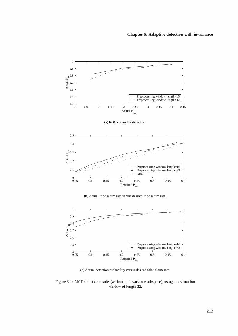
Chapter 6: Adaptive detection with invariance
0 0.05 0.1 0.15 0.2 0.25 0.3 0.35 0.4 0.450.4
0.5
0.6
0.7
0.8
0.9
1
Actual PFA
Act
ual P
D
Preprocessing window length=16Preprocessing window length=32
(a) ROC curves for detection.
0.05 0.1 0.15 0.2 0.25 0.3 0.35 0.40
0.1
0.2
0.3
0.4
0.5
Required PFA
Act
ual P
FA
Preprocessing window length=16Preprocessing window length=32Ideal
(b) Actual false alarm rate versus desired false alarm rate.
0.05 0.1 0.15 0.2 0.25 0.3 0.35 0.40.4
0.5
0.6
0.7
0.8
0.9
1
Required PFA
Act
ual P
D
Preprocessing window length=16Preprocessing window length=32
(c) Actual detection probability versus desired false alarm rate.
Figure 6.2: AMF detection results (without an invariance subspace), using an estimationwindow of length 32.
213
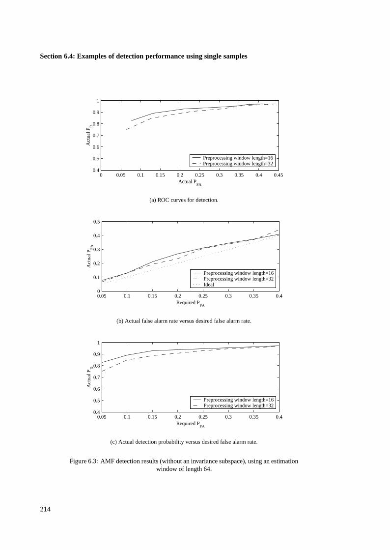
Section 6.4: Examples of detection performance using single samples
0 0.05 0.1 0.15 0.2 0.25 0.3 0.35 0.4 0.450.4
0.5
0.6
0.7
0.8
0.9
1
Actual PFA
Act
ual P
D
Preprocessing window length=16Preprocessing window length=32
(a) ROC curves for detection.
0.05 0.1 0.15 0.2 0.25 0.3 0.35 0.40
0.1
0.2
0.3
0.4
0.5
Required PFA
Act
ual P
FA
Preprocessing window length=16Preprocessing window length=32Ideal
(b) Actual false alarm rate versus desired false alarm rate.
0.05 0.1 0.15 0.2 0.25 0.3 0.35 0.40.4
0.5
0.6
0.7
0.8
0.9
1
Required PFA
Act
ual P
D
Preprocessing window length=16Preprocessing window length=32
(c) Actual detection probability versus desired false alarm rate.
Figure 6.3: AMF detection results (without an invariance subspace), using an estimationwindow of length 64.
214
Chapter 6: Adaptive detection with invariance
time using an estimation window of length 64.
A number of conclusions can be drawn from the results presented. Firstly, longer estimation windows
do not improve the performance of the test, either in terms of detectability (as shown by the ROC
curves) or predictability (as shown by the plots of actual versus required PFA). This can be attributed to
the fact that there is model mismatch, so the covariance estimates are biased. Increasing the estimation
window length does not decrease this bias.
Using more samples for estimation should however reduce the variance in the estimate, which could
bring about improved performance. However, this is not observed. A possible reason for this lack of
improvement is that the assumed model is not appropriate over the full length of the longer estimation
window. Thus the decreased variance is offset by inappropriateness of the model over longer sample
lengths.
Secondly, the difference between the required false alarm rate and the achieved false alarm rate is high.
This indicates that the assumed N [0, 1] distribution of the test statistic under H0 is not appropriate.
That is, even with long sequences of estimation data the expected asymptotic properties of the test are
not coming into play. Again this can be attributed to model mismatch, and the fact that the data are
not stationary across the length of the estimation window.
The conclusion may be drawn that even with the preprocessing, the assumption of an AR(1) process
along the length of the data windows being considered is inappropriate. The primary effect of the
mismatch is that the asymptotic properties of the test are not attained, and the detector is not predictable.
The invariant test formulation can be applied to the same problem. Because the model explicitly
incorporates mismatch, the preprocessing stage is not required. That is, the invariant detector simply
ignores those components which are in conflict with the model. An analysis of the invariant test was
performed as follows:
• Candidate invariance subspaces were estimated from the training image in Figure 5.11. Using a
subspace interference assumption, invariance subspaces of dimension 1, 3, and 5 were estimated
from the training data. The method used was the simultaneous approximate maximum likelihood
method presented in Section 5.7, using an assumed AR(1) model. The length of the invariance
subspace basis functions was chosen to be the same as the length of the estimation window. The
invariance subspaces were then assumed fixed, while the invariant detector was applied to the
test data.
• A similar procedure was then adopted as for the noninvariant adaptive detector discussed earlier.
In this case, however, the covariance matrix estimate was made to be invariant to the assumed
invariance subspace. For the calculation of both test statistic values, the covariance estimates
ignored the possible presence of a target. The test statistic tAMF from Equation 6.43 was used.
215
Section 6.4: Examples of detection performance using single samples
As with the noninvariant detector, this procedure results in two sets of sample values of the test statistic,
for the conditions of target presence and target absence. The sets of values were analysed in the same
manner as before. Figure 6.4 shows results for three different invariance subspace dimensions, and
an estimation window of length 32. Figure 6.5 shows similar results, but for an estimation window of
length 64.
The first point to note from these results is that the detectability of the test tends to decrease as the
invariance subspace is increased. This can be seen from the ROC curves, which move downwards for
higher invariance dimensions. This is a result of portions of the target lying in the invariance subspace,
and not being available for detection. However, the penalty incurred is far smaller for the case of a
longer estimation window length. This indicates that the longer estimation window has produced a
covariance estimate which is better than that obtained for shorter estimation windows. The only reason
that this improved estimation can be achieved is because the invariance subspace has improved the
validity of the model, even over long data lengths.
The second point of interest is that as the invariance subspace dimension is increased, the actual false
alarm rate tends towards the required rate. This makes for a very predictable detector, which performs
as designed. The presence of the invariance subspace has eliminated those components of the problem
where the data conflict with the AR(1) assumption. The bias in the covariance estimates is therefore
reduced, making the asymptotic properties of the test more appropriate.
6.4.2 Modified AMF results using single samples
In this section, similar results are provided to those of the previous section. The difference is that in
this case the modified AMF is used, which uses an average estimate of the covariance in the numerator.
Thus the adaptivity only comes in through the denominator term, which changes to suit the noise
properties of the particular sample of data being analysed.
For assessing the noninvariant detector for this problem, the same procedure used in the previous
section was adopted. The results for estimation windows of length 32 and 64 are shown in Figures 6.6
and 6.7. Shown in Figures 6.8 and 6.9 are analogous results for the modified AMF test when invariance
subspaces of different orders are included.
An interesting point in these plots is that in the nonadaptive case the longer preprocessing window
leads to better detectability, which is in contrast to the results presented in the previous section. The
predictability for this case is also improved, as demonstrated in the plots of required versus actual
false alarm rates. This result may well be specific to the target being detected. However, the reduced
uncertainty brought about by fixing the numerator of the test statistic has clearly improved the detection.
By fixing the detection statistic, the capacity of the test to adapt has been restricted. The test therefore
216
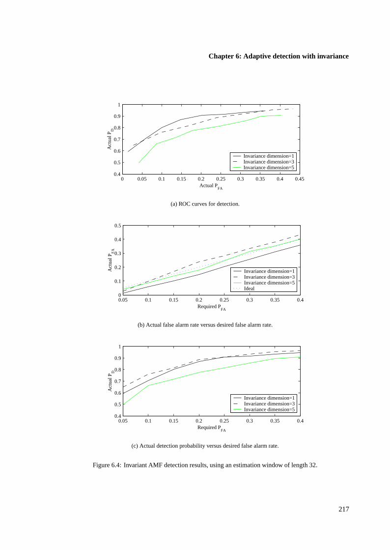
Chapter 6: Adaptive detection with invariance
0 0.05 0.1 0.15 0.2 0.25 0.3 0.35 0.4 0.450.4
0.5
0.6
0.7
0.8
0.9
1
Actual PFA
Act
ual P
D
Invariance dimension=1Invariance dimension=3Invariance dimension=5
(a) ROC curves for detection.
0.05 0.1 0.15 0.2 0.25 0.3 0.35 0.40
0.1
0.2
0.3
0.4
0.5
Required PFA
Act
ual P
FA
Invariance dimension=1Invariance dimension=3Invariance dimension=5Ideal
(b) Actual false alarm rate versus desired false alarm rate.
0.05 0.1 0.15 0.2 0.25 0.3 0.35 0.40.4
0.5
0.6
0.7
0.8
0.9
1
Required PFA
Act
ual P
D
Invariance dimension=1Invariance dimension=3Invariance dimension=5
(c) Actual detection probability versus desired false alarm rate.
Figure 6.4: Invariant AMF detection results, using an estimation window of length 32.
217
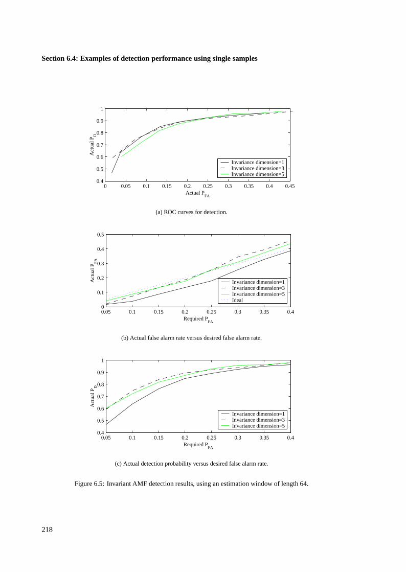
Section 6.4: Examples of detection performance using single samples
0 0.05 0.1 0.15 0.2 0.25 0.3 0.35 0.4 0.450.4
0.5
0.6
0.7
0.8
0.9
1
Actual PFA
Act
ual P
D
Invariance dimension=1Invariance dimension=3Invariance dimension=5
(a) ROC curves for detection.
0.05 0.1 0.15 0.2 0.25 0.3 0.35 0.40
0.1
0.2
0.3
0.4
0.5
Required PFA
Act
ual P
FA
Invariance dimension=1Invariance dimension=3Invariance dimension=5Ideal
(b) Actual false alarm rate versus desired false alarm rate.
0.05 0.1 0.15 0.2 0.25 0.3 0.35 0.40.4
0.5
0.6
0.7
0.8
0.9
1
Required PFA
Act
ual P
D
Invariance dimension=1Invariance dimension=3Invariance dimension=5
(c) Actual detection probability versus desired false alarm rate.
Figure 6.5: Invariant AMF detection results, using an estimation window of length 64.
218
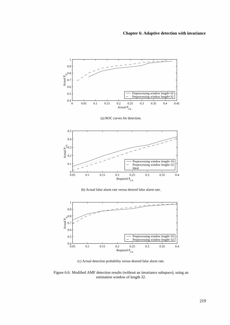
Chapter 6: Adaptive detection with invariance
0 0.05 0.1 0.15 0.2 0.25 0.3 0.35 0.4 0.450.4
0.5
0.6
0.7
0.8
0.9
1
Actual PFA
Act
ual P
D
Preprocessing window length=16Preprocessing window length=32
(a) ROC curves for detection.
0.05 0.1 0.15 0.2 0.25 0.3 0.35 0.40
0.1
0.2
0.3
0.4
0.5
Required PFA
Act
ual P
FA
Preprocessing window length=16Preprocessing window length=32Ideal
(b) Actual false alarm rate versus desired false alarm rate.
0.05 0.1 0.15 0.2 0.25 0.3 0.35 0.40.4
0.5
0.6
0.7
0.8
0.9
1
Required PFA
Act
ual P
D
Preprocessing window length=16Preprocessing window length=32
(c) Actual detection probability versus desired false alarm rate.
Figure 6.6: Modified AMF detection results (without an invariance subspace), using anestimation window of length 32.
219

Section 6.4: Examples of detection performance using single samples
0 0.05 0.1 0.15 0.2 0.25 0.3 0.35 0.4 0.450.4
0.5
0.6
0.7
0.8
0.9
1
Actual PFA
Act
ual P
D
Preprocessing window length=16Preprocessing window length=32
(a) ROC curves for detection.
0.05 0.1 0.15 0.2 0.25 0.3 0.35 0.40
0.1
0.2
0.3
0.4
0.5
Required PFA
Act
ual P
FA
Preprocessing window length=16Preprocessing window length=32Ideal
(b) Actual false alarm rate versus desired false alarm rate.
0.05 0.1 0.15 0.2 0.25 0.3 0.35 0.40.4
0.5
0.6
0.7
0.8
0.9
1
Required PFA
Act
ual P
D
Preprocessing window length=16Preprocessing window length=32
(c) Actual detection probability versus desired false alarm rate.
Figure 6.7: Modified AMF detection results (without an invariance subspace), using anestimation window of length 64.
220
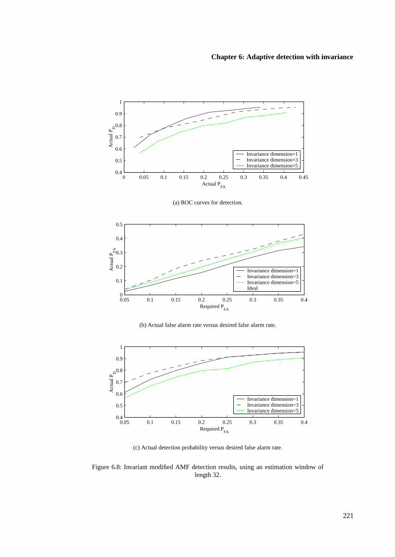
Chapter 6: Adaptive detection with invariance
0 0.05 0.1 0.15 0.2 0.25 0.3 0.35 0.4 0.450.4
0.5
0.6
0.7
0.8
0.9
1
Actual PFA
Act
ual P
D
Invariance dimension=1Invariance dimension=3Invariance dimension=5
(a) ROC curves for detection.
0.05 0.1 0.15 0.2 0.25 0.3 0.35 0.40
0.1
0.2
0.3
0.4
0.5
Required PFA
Act
ual P
FA
Invariance dimension=1Invariance dimension=3Invariance dimension=5Ideal
(b) Actual false alarm rate versus desired false alarm rate.
0.05 0.1 0.15 0.2 0.25 0.3 0.35 0.40.4
0.5
0.6
0.7
0.8
0.9
1
Required PFA
Act
ual P
D
Invariance dimension=1Invariance dimension=3Invariance dimension=5
(c) Actual detection probability versus desired false alarm rate.
Figure 6.8: Invariant modified AMF detection results, using an estimation window oflength 32.
221

Section 6.4: Examples of detection performance using single samples
0 0.05 0.1 0.15 0.2 0.25 0.3 0.35 0.4 0.450.4
0.5
0.6
0.7
0.8
0.9
1
Actual PFA
Act
ual P
D
Invariance dimension=1Invariance dimension=3Invariance dimension=5
(a) ROC curves for detection.
0.05 0.1 0.15 0.2 0.25 0.3 0.35 0.40
0.1
0.2
0.3
0.4
0.5
Required PFA
Act
ual P
FA
Invariance dimension=1Invariance dimension=3Invariance dimension=5Ideal
(b) Actual false alarm rate versus desired false alarm rate.
0.05 0.1 0.15 0.2 0.25 0.3 0.35 0.40.4
0.5
0.6
0.7
0.8
0.9
1
Required PFA
Act
ual P
D
Invariance dimension=1Invariance dimension=3Invariance dimension=5
(c) Actual detection probability versus desired false alarm rate.
Figure 6.9: Invariant modified AMF detection results, using an estimation window oflength 64.
222
Chapter 6: Adaptive detection with invariance
works well in the case of the data under analysis here, which are quite homogeneous. For more
variable data the lack of adaptivity will incur a performance penalty. Nonetheless, the results indicate
that adaptivity in general causes a decrease in performance, as a result of having to make estimates of
the required parameters. Thus detectors should only be made as adaptive as necessary.
The invariant detector works quite well in this case, especially with regard to predictability. The
detection performance does suffer, however, again as a result of part of the target being ignored in the
detection. The observation can once again be made that the longer estimation window lengths improve
the overall performance, a factor which can be directly attributed to the invariance subspace making
the assumed model appropriate over longer data lengths.
Finally, the last plot in Figure 6.9 demonstrates how improved predictability can lead directly to
improved detectability, purely as a result of being able to set the test threshold more accurately. As the
invariance subspace increases the detectability decreases, but through better threshold specification the
more invariant detector can ultimately produce higher detectability as a function of the required false
alarm rate.
6.4.3 Target-invariant AMF results using single samples
The final results demonstrate the use of the target-invariant method for estimating the covariance matrix
used in the invariant AMF. These are provided in Figures 6.10 and 6.11. Here the covariance estimate
is completely independent of the possible presence of a target. The results are marginally better than
the test which assumes only noise present in the estimation data, but the difference is slight.
This improvement is small primarily because of the tight constraint on the noise model. That is, the
presence of a short duration transient target in the signal is almost completely ignored in the estimation,
since it conflicts very strongly with the assumed set of possible distributions. The noninvariant esti-
mation therefore does not suffer greatly from the presence of this target. For different targets, which
more closely resemble realisations of the low-order random process, this may no longer be the case.
Also, less restrictive noise models may be more affected by the presence of the target.
223
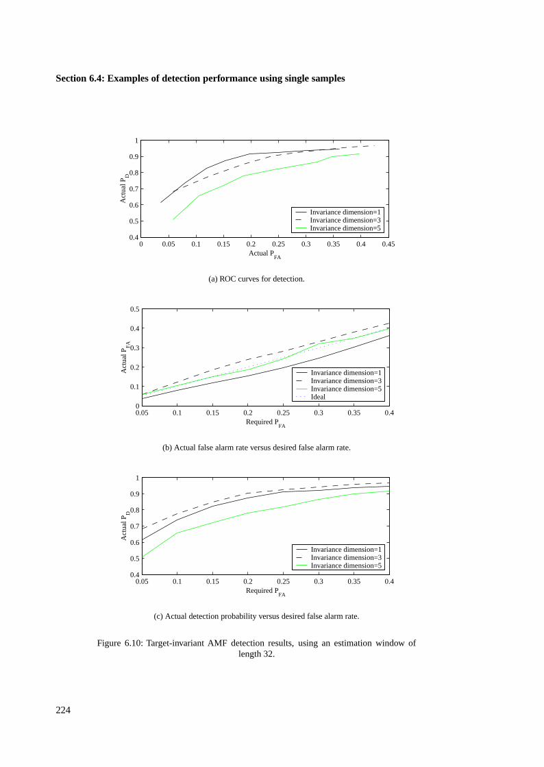
Section 6.4: Examples of detection performance using single samples
0 0.05 0.1 0.15 0.2 0.25 0.3 0.35 0.4 0.450.4
0.5
0.6
0.7
0.8
0.9
1
Actual PFA
Act
ual P
D
Invariance dimension=1Invariance dimension=3Invariance dimension=5
(a) ROC curves for detection.
0.05 0.1 0.15 0.2 0.25 0.3 0.35 0.40
0.1
0.2
0.3
0.4
0.5
Required PFA
Act
ual P
FA
Invariance dimension=1Invariance dimension=3Invariance dimension=5Ideal
(b) Actual false alarm rate versus desired false alarm rate.
0.05 0.1 0.15 0.2 0.25 0.3 0.35 0.40.4
0.5
0.6
0.7
0.8
0.9
1
Required PFA
Act
ual P
D
Invariance dimension=1Invariance dimension=3Invariance dimension=5
(c) Actual detection probability versus desired false alarm rate.
Figure 6.10: Target-invariant AMF detection results, using an estimation window oflength 32.
224
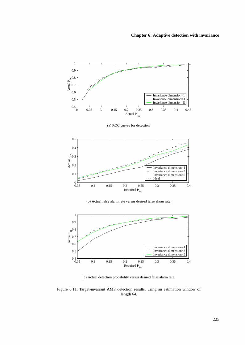
Chapter 6: Adaptive detection with invariance
0 0.05 0.1 0.15 0.2 0.25 0.3 0.35 0.4 0.450.4
0.5
0.6
0.7
0.8
0.9
1
Actual PFA
Act
ual P
D
Invariance dimension=1Invariance dimension=3Invariance dimension=5
(a) ROC curves for detection.
0.05 0.1 0.15 0.2 0.25 0.3 0.35 0.40
0.1
0.2
0.3
0.4
0.5
Required PFA
Act
ual P
FA
Invariance dimension=1Invariance dimension=3Invariance dimension=5Ideal
(b) Actual false alarm rate versus desired false alarm rate.
0.05 0.1 0.15 0.2 0.25 0.3 0.35 0.40.4
0.5
0.6
0.7
0.8
0.9
1
Required PFA
Act
ual P
D
Invariance dimension=1Invariance dimension=3Invariance dimension=5
(c) Actual detection probability versus desired false alarm rate.
Figure 6.11: Target-invariant AMF detection results, using an estimation window oflength 64.
225

Section 6.4: Examples of detection performance using single samples
226
Chapter 7
Conclusion
Section 7.1 summarises the main topics and results in this thesis. Section 7.2 then makes some general
conclusions based on the work.
7.1 Summary of main topics
The primary goal of this thesis is to demonstrate some of the roles that invariance and constraints
can play in detection problems. Two types of invariance are considered, namely invariance to cyclic
permutations, and invariance to components of the data contained in linear subspaces of the observation
space.
The GLRT plays an important part in applied target detection, and this work is no exception. Chapter 3
addresses the issue of suboptimality of the GLRT for simple detection of targets with unknown location
in certain types of noise. Specifically, a UMPI test is developed for the case where the target is known
and the covariance circulant. This test is most powerful in the class of all cyclic permutation invariant
tests. Since the GLRT falls into this class, a direct comparison of the two tests is possible. It is shown
that for circulant covariances the differences between the GLRT and the optimal UMPI test are small.
This justifies the use of the more conventional GLRT for the testing problem.
Another issue that is addressed is the use of invariance for eliminating nuisance parameters. For certain
unknown target location problems, it is demonstrated that cyclic permutation invariance is a natural
restriction to impose, and even when additional unknown parameters are present, the resulting test can
be more powerful than the corresponding noninvariant test. The specific case of detection in noise
with unknown power is discussed in detail. A cyclic permutation invariance condition is imposed, and
an invariant estimate of the noise power used to specify the test. The test which includes invariance is
again shown to be more powerful than the conventional GLRT for the problem.
227
Section 7.1: Summary of main topics
The second application of invariance concerns invariance to data components contained in linear
subspaces of the observation space. In Chapter 4 subspace invariant tests are formulated, and methods
provided for calculating the resulting test statistics. This form of invariant testing is applied to two
problems, namely that of detection in subspace interference, and detection in noise which is difficult
to characterise.
For both these situations, methods are presented for estimating candidate invariance subspaces under
the assumption that the covariance matrix is known. In the first instance a maximum likelihood
formulation is proposed, where the invariance subspace serves to eliminate those components of the
data which can be modelled least accurately. In the second instance, a method based on the Frobenius
distance between covariances contained in certain subspaces is used, where the invariance subspace
serves to ignore the dimensions where the conflict between the assumed model and the actual data is
greatest. It is demonstrated that both of these methods lead to useful estimates.
In particular, simulated results are provided for the case of interference subspace identification. The
estimates are shown to be accurate. However, on account of approximations that had to be made in
the derivation of the estimates, they are not ideal because they are not consistent. Nevertheless, they
work well in instances where the interference components are large. A demonstration of the use of
an invariance subspace for reducing model mismatch is presented for a real-data application, and it is
shown that the resulting estimate improves both the detectability and predictability of the hypothesis
test.
Chapter 5 discusses the problem of estimating covariance matrices for use in invariant detectors. It is
argued that when the covariance matrices are constrained, the estimates are required to be invariant
to the same subspace as the detector. For the subspace invariance problem, an invariant maximum
likelihood paradigm is proposed, where only the data contained in subspaces complementary to the
invariance subspace are used in the estimation. Detailed methods are presented for calculating the
covariance estimates under circulant, Toeplitz, doubly block circulant, doubly block Toeplitz, and
ARMA constraints.
It is shown that when the covariance matrix is unconstrained, explicit invariance in the estimate is not
required. When constraints are present, however, this is no longer true, since the data components in
the invariance subspace corrupt the estimate in a way which is not ignored in the subsequent detection.
The problem of simultaneous covariance and invariance subspace estimation is then addressed, and
methods provided for obtaining such estimates under the assumption that the noise largely obeys an
ARMA model. Practical examples are provided demonstrating the use of these estimates for actual
problems. Simulations are again provided showing the performance for the subspace interference
interpretation, and the results shown to be good. The methods are also applied to actual data, both in
the context of subspace interference and subspace invariance for model mismatch reduction. The use
of an invariance subspace is shown to improve the predictability of the resulting detectors, and in some
228

Chapter 7: Conclusion
cases to improve the detectability. Perhaps more importantly, explicit use of an invariance subspace
can improve the ability of the detector to generalise beyond the set of training data.
The improved predictability is of particular importance in adaptive detection, where the noise estimates
are used to yield approximately CFAR properties. The use of subspace invariance for this application
is discussed in Chapter 6. The chapter opens by providing a decomposition of the subspace invariant
testing problem into relevant subspaces, which has application in interpreting the roles of the various
components of the observations. The AMF and the GLRT, which assume the presence of secondary
noise-only observations, are then modified for the case of a known target with unknown amplitude,
where the amplitude is restricted to be positive. This is a more natural formulation for many problems
involving detection in real data, and the resulting tests are shown to be more powerful than those which
consider the amplitude parameter completely unknown. The tests have a CFAR property, even when
a known invariance subspace is included.
It is argued that for some applications it is reasonable to make a single invariance subspace estimate,
and hold this fixed for the remainder of the adaptive testing. The invariance subspace then just serves
to improve the modelling on the average. The modified AMF and GLRT formulations are discussed
for the case where constraints in the covariance are enforced, and the special case is discussed where
the same data are used for parameter estimation and detection. In these cases the tests are not strictly
CFAR, but tend to become so as the parameter estimation improves.
The use of invariance to possible target presence is then proposed as a method of improving perfor-
mance, or reducing computational requirements, particularly in the case of constrained covariances. It
is shown that if target-invariant estimates are used in the tests, then the problem of invalid assumptions
in the estimation is overcome. This should lead to improved detectability, expecially if the target
amplitude is large.
Partially adaptive detectors are also proposed, where the test threshold is adapted but the basic statistic
is held constant. These tests have an advantage in that a costly matrix inversion is eliminated. They also
lead to CFAR tests in the unconstrained covariance case, and asymptotically CFAR tests otherwise.
The specific case of simultaneous estimation and detection from a single sample of data is discussed
in detail, particularly with regard to the AMF, GLRT, and simplified AMF. A covariance constraint is
essential in these cases, and the tests become CFAR as the parameter estimates improve. The AMF
and modified AMF are also applied to a sample of real data, both in noninvariant and invariant forms.
The invariant test formulations are shown to have improved predictability, which comes at the cost of
slightly reduced detectability. In some cases this improved predictability can, however, lead to tests
which perform better on the whole.
229
Section 7.2: General conclusions
7.2 General conclusions
The results of Chapter 3 partially validate the use of the GLRT for detection problems where the
location of the target is unknown. For some very simple situations, the performance of the GLRT is
almost as good as the optimal test for the problem. It is only possible to compare the GLRT to the
optimal test under a restricted set of circumstances, but these are sufficiently similar to more common
situations to make the comparison useful as a baseline.
In practice, unknown target location problems arise frequently, and are usually dealt with in an ad
hoc manner. By explicitly introducing an unknown location parameter, however, the assumed model
represents the actual situation being modelled far more accurately. If the problem formulation then
has a reasonable solution, it is of considerably more value than a solution which assumes the location
known. Admittedly, complications arising from the introduction of such a parameter may greatly
hinder the search for a solution. On the other hand, it forces the system designer to at least consider
the effect that the unknown location actually has on the problem. In the literature, detectors designed
for known target location problems are often applied in a sliding window framework, with little or no
consideration given to associated problems which might arise.
More importantly, in this thesis, is the role that invariance can play in the problem. It is demonstrated
that when a nuisance parameter can be eliminated though a legitimate invariance criterion, the resulting
detection performance almost always improves. This stems directly from the fact that the parameter
otherwise has to be estimated, which increases the uncertainty in the test statistic. However, invariant
detectors introduce other difficulties, namely the need for invariant estimators. Under a maximum
likelihood framework these detectors may be quite easy to specify, but their calculation may not be
trivial.
The results of Chapters 4 and 5 address a related issue. In particular, the use of invariance to a certain
subspace of the data is proposed. The first application is to the problem of detection in subspace
interference. Under the condition that the interference lies in a known subspace but is otherwise
unknown, an invariant detector can be derived which is optimal in a UMPI sense. In practice, however,
the interference subspace is seldom known, and even the assumption that the components contained
in this subspace are completely unknown is questionable. Nevertheless, the subspace interference
assumption may still be adopted, albeit in a non-optimal context.
To this end, methods of estimating candidate interference subspaces are presented. These methods
are more general than required, in that they do not take into account the fact that the interference
components must always enter into the sample covariance through a positive definite matrix. Rather
than considering this a shortcoming, however, it can be argued that it improves the applicability of
the subspace invariance formalism to applications beyond those of strict subspace interference. The
methods also do not require an assumption of multivariate normality of the covariance in the noise-
230
Chapter 7: Conclusion
plus-interference process, which extends the applicability.
The fact that an exact maximum likelihood method has not been found for the interference subspace
estimation problem is problematic, particularly when joint estimation of the subspace and the co-
variance matrix is required. Nevertheless, the approximate methods appear to work when applied to
real-data problems. Indeed, the fact that they work so well is surprising, particularly when a subspace
interference interpretation on the data is questionable. In short, a noise plus subspace interference
model seems quite appropriate for modelling a wide variety of data.
The use of invariance to explicitly reduce model mismatch is unique, and could have application to
problems far beyond those discussed in this thesis. In particular, apart from computational convenience
there is no reason to restrict the notion to subspace invariance. By imposing equivalence classes on
those portions of the data which are in conflict with some convenient modelling assumption, better
performance may be achieved than if the mismatch is simply ignored. This improvement does however
come at the risk of reduced detectability, if the application of invariance substantially eliminates part
of the target.
The use of subspace invariance for model mismatch is quite tractable, on account of the simple relation-
ships between MVN distributions and linear transformations. In the example given in Section 4.5.2 it
is quite clear that the presence of such an invariance subspace leads to a considerably more predictable
detector.
Once again the presence of invariance raises the need for invariant estimators. Conceptually there is
nothing complicated about such detectors — they can simply be obtained by performing the estimation
based on the maximal invariant statistic rather than on the original data. They may however be difficult
to calculate. The complexity of the methods presented in Chapter 5 attribute to this fact.
The invariant detectors proposed are particularly useful in situations where computational efficiency is
paramount. Using the methods discussed, a single simple detection statistic is obtained which is robust
to certain expected deviations of the data from the assumed model. The resulting detection statistic
can be calculated using a simple convolution product, if used in a sliding window context. Thus the
need for adaptivity or preprocessing can sometimes be avoided. Avoiding adaptivity is desirable from
a computational perspective. Avoiding preprocessing is desirable since it introduces a second stage of
modelling and computation, which increases the uncertainty in the results.
The methods presented for simultaneous estimation of invariance subspaces and covariance matri-
ces are quite limiting, in that explicit maximisation of the likelihood is indicated. Nevertheless, for
many applications ARMA models are sufficiently rich to successfully model data, particularly when
an invariance subspace is included to accommodate any mismatch. Being stationary, they can also
successfully identify primary causes of nonstationarity in data, which to a large extent is what the in-
variance subspace is required for. Additionally, since the invariance subspace identification procedure
231
Section 7.2: General conclusions
can be performed off-line, methods with high computational complexity are not inappropriate.
The Toeplitz and circulant constraints on the covariance are primarily of interest in applications where
there is a large amount of data from which to make estimates. In many practical problems, this condition
is not met. When detectors are made adaptive, the computational requirements can also be prohibitive,
at least with computing technology where it now stands. Nonetheless, as far as multiple-observation
detection is concerned, the use of constraints is important and can improve detectability substantially.
Chapter 6 outlines many of the uses of subspace invariance and invariant covariance estimation in a
detection context. The opening analysis regarding the roles of the target, invariance, and noise-only
subspaces is conceptually invaluable, particularly when detection and estimation are to be performed
using the same data sample.
Subspace invariance can extend the application of multiple-observation detector formulations to cases
where the observations do not come from identical processes, as long as the processes differ only in
their distribution in a restricted linear subspace. Under both the AMF and GLRT formulations the
invariant tests continue to be CFAR.
Also, subspace invariance can extend the lengths of data over which a stationarity assumption can be
assumed valid, by ignoring the primary causes of nonstationarity. This is particularly important when
tests are only asymptotically CFAR, with an intractable or unknown distribution for the test statistic.
Parameter estimates should then be as accurate as possible for asymptotic results to be used effectively.
The improved modelling accuracy brought about by the inclusion of an invariance subspace translates
directly to more predictable tests. That is, the actual attained false alarm rates correspond far more
closely to the false alarm rates specified in the design. This is important in any application where a
false alarm can be considered costly, perhaps in the form of a subsequent action which then has to be
taken. In these contexts the reduced detectability may be fully justified.
The presence of an invariance subspace also partially eliminates the need for preprocessing of the data,
particularly when highly-constrained models are considered. As demonstrated in the results, a method
of preprocessing which is appropriate for one detector may not be appropriate for a different detector,
even if the two are quite similar. Also, preprocessing is usually fairly ad hoc, with no systematic
method available for designing a good solution. The invariant detectors, however, compensate for
modelling inaccuracies in the calculation of the test statistic itself, where they can be analysed as part
of the detector specification. In general, when it can be achieved, this provides a far better solution.
The analysis of the modified AMF, which does not involve adaptivity in the numerator term, provides
insight into the price that has to be paid for adaptivity in a detector. In effect, every term in the test
expression that has to be estimated contributes uncertainty into the resulting value. Thus tests should
only be made as adaptive is necessary.
232

The subspace methods presented in this work do not provide a final solution to any given testing
problem. Rather, they provide additional tools which may sometimes be used to design detectors for
certain problems, which otherwise would be difficult to solve. In this sense, they just increase the set
of possible detectors which may be considered for a problem. The methods cannot be applicable in
all problems, however. It is up to the system designer to ascertain whether the methods have merit for
any particular problem which is under investigation.
Finally, the methods presented in this work have been based on maximum likelihood principles primar-
ily in the interests of rigour. The maximum likelihood framework is a good paradigm for investigating
ideas, but the computational complexity can limit the application somewhat. When applied in real
situations, it may often be expected that less complicated estimates will suffice for certain components
of the detection problems.
233

234
Bibliography
[1] A. A. ABU-DAYYA AND N. C. BEAULIEU. Outage probabilities in the presence of correlated
lognormal interferers. IEEE Transactions on Vehicular Technology, 43(1):164–173, February
1994.
[2] H. AKAIKE. Maximum likelihood identification of Gaussian autoregressive moving average
models. Biometrika, 60(2):255–265, 1973.
[3] C. F. ANSLEY. An algorithm for the exact likelihood of a mixed autoregressive-moving average
process. Biometrika, 66(1):59–65, 1979.
[4] H. ANTON. Elementary Linear Algebra. John Wiley & Sons, sixth edition, 1991.
[5] P. M. BAGGENSTOSS AND S. M. KAY. An adaptive detector for deterministic signals in noise
of unknown spectra using the rao test. IEEE Transactions on Signal Processing, 40(6):1460–
1468, June 1992.
[6] A. BASILEVSKY. Applied Matrix Algebra in the Statistical Sciences. Elsevier Science Pub-
lishing Company, 1983.
[7] N. C. BEAULIEU, A. A. ABU-DAYYA, AND P. J. MCLANE. Estimating the distribution of
a sum of independent lognormal random variables. IEEE Transaction on Communications,
43(12):2869–2873, December 1995.
[8] A. A. L. BEEX AND M. P. FARGUES. Highly parallel recursive/iterative Toeplitz eigenspace
decomposition. IEEE Transactions on Acoustics, Speech, and Signal Processing, 37(11):1765–
1768, November 1989.
[9] R. T. BEHRENS AND L. L. SCHARF. Signal processing applications of oblique projection
operators. IEEE Transactions on Signal Processing, 42(6):1412–1424, June 1994.
[10] J. O. BERGER. Statistical Decision Theory: Foundations, concepts, and methods. Springer
Series in Statistics. Springer-Verlag, 1980.
[11] C. M. BISHOP. Neural Networks for Pattern Recognition. Oxford University Press, 1995.
235
[12] S. BOSE AND A. O. STEINHARDT. A maximal invariant framework for adaptive detection
with structured and unstructured covariance matrices. IEEE Transactions on Signal Processing,
43(9):2164–2175, September 1995.
[13] S. BOSE AND A. O. STEINHARDT. Adaptive array detection of uncertain rank one waveforms.
IEEE Transactions on Signal Processing, 44(11):2801–2809, November 1996.
[14] D. E. BOWYER, P. K. RAJASEKARAN, AND W. W. GEBHART. Adaptive clutter filtering using
autoregressive spectral estimation. IEEE Transactions on Aerospace and Electronic Systems,
AES-15(4):538–546, July 1979.
[15] G. E. P. BOX, G. M. JENKINS, AND G. C. REINSEL. Time Series Analysis: Forecasting and
Control. Prentice-Hall, third edition, 1994.
[16] L. E. BRENNAN AND I. S. REED. Theory of adaptive radar. IEEE Transactions on Aerospace
and Electronic Systems, AES-9(2):237–252, March 1973.
[17] P. J. BROCKWELL AND R. A. DAVIS. Time series: theory and methods. Springer Series in
Statistics. Springer-Verlag, second edition, 1991.
[18] P. J. BROCKWELL AND R. A. DAVIS. Introduction to Time Series and Forecasting. Springer
Texts in Statistics. Springer-Verlag, 1996.
[19] J. P. BURG, D. G. LUENBERGER, AND D. L. WENGER. Estimation of structured covariance
matrices. Proceedings of the IEEE, 70(9):963–974, September 1982.
[20] K. A. BURGESS AND B. D. VAN VEEN. Subspace-based adaptive generalized likelihood ratio
detection. IEEE Transactions on Signal Processing, 44(4):912–927, April 1996.
[21] D. BURSHTEIN. An efficient algorithm for calculating the likelihood and likelihood gradient
of ARMA models. IEEE Transactions on Automatic Control, 38(2):336–340, February 1993.
[22] J. Y. CHEN AND I. S. REED. A detection algorithm for optical targets in clutter. IEEE
Transactions on Aerospace and Electronic Systems, AES-23(1):46–59, January 1987.
[23] G. CORTELAZZO, G. A. MIAN, AND R. RINALDO. Toeplitz properties of the block ma-
trices encountered in the processing of spatiotemporal signals. IEEE Transactions on Signal
Processing, 39(7):1672–1674, July 1991.
[24] P. J. DAVIS. Circulant Matrices. Pure & Applied Mathematics: A Wiley-Interscience Series
of Texts, Monographs & Tracts. John Wiley & Sons, 1979.
[25] M. H. DEGROOT. Probability and Statistics. Addison-Wesley Series in Statistics. Addison-
Wesley, second edition, 1986.
236
[26] A. S. DEIF. Advanced Matrix Theory for Scientists and Engineers. John Wiley & Sons, 1982.
[27] A. DEMBO, C. L. MALLOWS, AND L. A. SHEPP. Embedding nonnegative definite Toeplitz
matrices in nonnegative definite circulant matrices, with application to covariance estimation.
IEEE Transactions on Information Theory, 35(6):1206–1212, November 1989.
[28] A. P. DEMPSTER, N. M. LAIRD, AND D. B. RUBIN. Maximum likelihood from incomplete
data via the EM algorithm. Journal of the Royal Statistical Society: B, 39:1–38, 1977.
[29] G. M. DILLARD. Mean-level detection of nonfluctuating signals. IEEE Transactions on
Aerospace and Electronic Systems, AES-10(6):795–799, November 1984.
[30] M. L. EATON. Multivariate Statistics: A Vector Space Approach. Wiley Series in Probability
and Mathematical Statistics. John Wiley & Sons, 1983.
[31] M. H. EL AYADI. Generalised likelihood adaptive detection of signals deformed by unknown
linear filtering in noise with slowly fluctuating power. IEEE Transactions on Acoustics, Speech,
and Signal Processing, ASSP-33(2):401–405, April 1985.
[32] M. H. EL AYADI. NAR estimators of spatial covariance matrices for adaptive array detection.
IEEE Transactions on Signal Processing, 39(7):1682–1686, July 1991.
[33] M. H. EL AYADI AND B. PICINBONO. NAR AGC adaptive detection of nonoverlapping signals
in noise with fluctuating power. IEEE Transactions on Acoustics, Speech, and Signal Processing,
ASSP-29(5):952–963, October 1981.
[34] T. S. FERGUSON. Mathematical Statistics: A decision theoretic approach. Probability in
Mathematical statistics. Academic Press, 1967.
[35] B. FRIEDLANDER AND B. PORAT. Performance analysis of transient detectors based on a class
of linear data transforms. IEEE Transactions on Information Theory, 38(2):665–673, March
1992.
[36] M. FRISCH AND H. MESSER. The use of the wavelet transform in the detection of an unknown
transient signal. IEEE Transactions on Information Theory, 38(2):892–897, March 1992.
[37] M. FRISCH AND H. MESSER. Transient signal detection using prior information in the likeli-
hood ratio test. IEEE Transactions on Signal Processing, 41(6):2177–2192, June 1993.
[38] M. FRISCH AND H. MESSER. Detection of a known transient signal of unknown scaling and
arrival time. IEEE Transactions on Signal Processing, 42(7):1859–1863, July 1994.
[39] D. R. FUHRMANN. Application of Toeplitz covariance estimation to adaptive beamforming
and detection. IEEE Transactions on Signal Processing, 39(10):2194–2198, October 1991.
237
[40] K. FUKUNAGA. Introduction to Statistical Pattern Recognition. Computer Science and Scien-
tific Computing. Academic Press, second edition, 1990.
[41] W. A. FULLER. Introduction to Statistical Time Series. Wiley Series in Probability and Statistics.
John Wiley & Sons, second edition, 1996.
[42] W. A. GARDNER AND C. M. SPOONER. The cumulant theory of cyclostationary time-series,
part I: foundations. IEEE Transactions on Signal Processing, 42(12):3387–3408, December
1994.
[43] N. GASTINEL. Linear Numerical Analysis. Hermann, 1970. Translated from the original
French text Analyse numérique linéaire, first published by Hermann in 1966.
[44] Y.-L. GAU AND I. S. REED. An improved reduced-rank CFAR space-time adaptive radar
detection algorithm. IEEE Transactions on Signal Processing, 46(8):2139–2146, August 1998.
[45] N. C. GEÇKINLI AND D. YAVUZ. Discrete Fourier Transformation and Its Applications to
Power Spectra Estimation, volume 8 of Studies in Electrical and Electronic Engineering. Else-
vier, 1983.
[46] D. F. GINGRAS AND E. MASRY. Autoregressive spectral estimation in additive noise. IEEE
Transactions on Acoustics, Speech, and Signal Processing, 36(4):490–501, April 1988.
[47] G. H. GOLUB AND C. F. VAN LOAN. Matrix Computations. Johns Hopkins University Press,
1983.
[48] G. H. GOLUB AND C. F. VAN LOAN. Matrix Computations. Johns Hopkins Series in the
Mathematical Sciences. Johns Hopkins University Press, third edition, 1996.
[49] A. GRAHAM. Kronecker Products and Matrix Calculus. Ellis Horwood Series in Mathematics
and its Applications. Halsted Press, 1981.
[50] R. M. GRAY. On the asymptotic eigenvalue distribution of Toeplitz matrices. IEEE Transactions
on Information Theory, IT-18(6):725–730, November 1972.
[51] U. GRENANDER AND G. SZEGÖ. Toeplitz Forms and their Applications. University of Cali-
fornia Press, 1958.
[52] M. GUIDA, M. LONGO, AND M. LOPS. Biparametric CFAR procedures for lognormal clutter.
IEEE Transactions on Aerospace and Electronic Systems, 29(3):798–809, July 1993.
[53] D. V. GUPTA, J. F. VETELINO, T. J. CURRY, AND J. T. FRANCIS. An adaptive threshold
system for nonstationary noise backgrounds. IEEE Transactions on Aerospace and Electronic
Systems, AES-13(1):11–16, January 1977.
238
[54] M. A. HAMDAN. The logarithm of the sum of two correlated log-normal variates. Journal of
the American Statistical Association, 66(333):105–106, March 1971.
[55] M. HAMERMESH. Group Theory and its Application to Physical Problems. Addison-Wesley,
1962.
[56] M. H. HAYES. The reconstruction of a multidimensional sequence from the phase or magnitude
of its Fourier transform. IEEE Transactions on Acoustics, Speech, and Signal Processing, ASSP-
30(2):140–154, April 1982.
[57] S. S. HAYKIN, editor. Array Signal Processing. Prentice-Hall, 1985.
[58] S. S. HAYKIN. Neural Networks: A Comprehensive Foundation. Prentice-Hall, second edition,
1999.
[59] C. W. HELSTROM. Statistical Theory of Signal Detection. Pergamon Press, 1960.
[60] A. HERO. Hilights of statistical signal and array processing. IEEE Signal Processing Magazine,
pages 21–64, September 1998.
[61] S. D. HIMONAS AND M. BARKAT. Adaptive CFAR detection in partially correlated clutter.
IEE Proceedings, Pt F, 137(5):387–394, October 1990.
[62] R. V. HOGG AND A. T. CRAIG. Introduction to Mathematical Statistics. Macmillan, third
edition, 1970.
[63] R. A. HORN AND C. R. JOHNSON. Topics in Matrix Analysis. Cambridge University Press,
1991.
[64] D. HUANG. Symmetric solutions and eigenvalue problems of Toeplitz systems. IEEE Trans-
actions on Signal Processing, 40(12):3069–3074, December 1992.
[65] A. K. JAIN. Fundamentals of Digital Image Processing. Prentice-Hall, 1989.
[66] W. A. JANOS. Tail of the distribution of sums of log-normal variates. IEEE Transactions on
Information Theory, IT-16(3):299–302, May 1970.
[67] W. B. JONES AND O. NJØASTAD. Applications of Szegö polymonials to digital signal pro-
cessing. Rocky Mountain Journal of Mathematics, 21(1):387–436, 1991.
[68] W. B. JONES, O. NJØASTAD, AND E. B. SAFF. Szegö polynomials associated with Wiener-
Levinson filters. Journal of Computational and Applied Mathematics, 32:387–406, 1990.
[69] G. G. JUDGE, W. E. GRIFFITHS, R. CARTER HILL, H. LÜTKEPOHL, AND T.-C. LEE. The
Theory and Practice of Econometrics. Wiley Series in Probability and Statistics. John Wiley &
Sons, second edition, 1985.
239
[70] J. H. JUSTICE. An algorithm for inverting positive definite Toeplitz matrices. SIAM Journal
on Applied Mathematics, 23(3):289–291, November 1972.
[71] J. H. JUSTICE. A Levinson-type algorithm for two-dimensional Weiner filtering using bivariate
Szegö polynomials. Proceedings of the IEEE, 65(6):882–886, June 1977.
[72] S. A. KASSAM AND H. V. POOR. Robust techniques for signal processing: a survey. Proceed-
ings of the IEEE, 73(3):433–481, March 1985.
[73] S. M. KAY. Noise compensation for autoregressive spectral estimates. IEEE Transactions on
Acoustics, Speech, and Signal Processing, ASSP-28(3):292–303, June 1980.
[74] S. M. KAY. Asymptotically optimal detection in unknown colored noise via autoregressive
modeling. IEEE Transactions on Acoustics, Speech, and Signal Processing, ASSP-31(4):927–
940, August 1983.
[75] S. M. KAY. Modern Spectral Estimation: Theory and Applications. Prentice-Hall, 1988.
[76] S. M. KAY. Asymptotically optimal detection in incompletely characterised non-Gaussian
noise. IEEE Transactions on Acoustics, Speech, and Signal Processing, 37(5):627–633, May
1989.
[77] S. M. KAY. Fundamentals of Statistical Signal Processing: Estimation Theory. Prentice Hall
Signal Processing Series. Prentice-Hall, 1993.
[78] S. M. KAY AND S. L. MARPLE, JR. Spectrum analysis — a modern perspective. Proceedings
of the IEEE, 69(11):1380–1419, November 1981.
[79] D. KAZAKOS AND P. PAPANTONI-KAZAKOS. Detection and Estimation. Computer Science
Press, 1990.
[80] E. J. KELLY. An adaptive detection algorithm. IEEE Transactions on Aerospace and Electronic
Systems, AES-22(1):115–127, March 1986.
[81] M. KENDALL AND A. STUART. The Advanced Theory of Statistics, volume 2. Charles Griffin
& Company, fourth edition, 1979.
[82] C. G. KHATRI AND C. RADHAKRISHNA RAO. Effects of estimated noise covariance matrix
in optimal signal detection. IEEE Transactions on Acoustics, Speech, and Signal Processing,
ASSP-35(5):671–679, May 1987.
[83] I. P. KIRSTEINS AND D. W. TUFTS. Adaptive detection using low rank approximation to a
data matrix. IEEE Transactions on Aerospace and Electronic Systems, 30(1):55–67, January
1994.
240
[84] H. KRIM AND M. VIBERG. Two decades of array signal processing research. IEEE Signal
Processing Magazine, pages 67–94, July 1996.
[85] P. LANCASTER. Theory of Matrices. Academic Press, 1969.
[86] H. J. LARSON. Introduction to Probability Theory and Statistical Inference. Wiley Series in
Probability and Mathematical Statistics. John Wiley & Sons, third edition, 1982.
[87] E. L. LEHMANN. Testing Statistical Hypotheses. Wiley Series in Probability and Mathematical
Statistics. John Wiley & Sons, second edition, 1986.
[88] R. LENZ. Group Theoretical Methods in Image Processing, volume 413 of Lecture Notes in
Computer Science. Springer-Verlag, 1990.
[89] R. J. A. LITTLE AND D. B. RUBIN. Statistical Analysis with Missing Data. Wiley Series in
Probability and Mathematical Statistics. John Wiley & Sons, 1987.
[90] J. MAKHOUL. Linear prediction: a tutorial review. Proceedings of the IEEE, 63(4):561–580,
April 1975.
[91] J. MAKHOUL. On the eigenvectors of symmetric Toeplitz matrices. IEEE Transactions on
Acoustics, Speech, and Signal Processing, ASSP-29(4):868–872, August 1981.
[92] A. MARGALIT, I. S. REED, AND R. M. GAGLIARDI. Adaptive optical target detection using
correlated images. IEEE Transactions on Aerospace and Electronic Systems, AES-21(3):394–
405, May 1985.
[93] G. J. MCLACHLAN. Discriminant Analysis and Statistical Pattern Recognition. Wiley Series
in Probability and Mathematical Statistics. John Wiley & Sons, 1992.
[94] G. MÉLARD. A fast algorithm for the exact likelihood of autoregressive-moving average models.
Applied Statistics, 33(1):104–114, 1984.
[95] M. I. MILLER, D. R. FUHRMANN, J. A. O’SULLIVAN, AND D. L. SNYDER. Maximum-
likelihood methods for Toeplitz covariance estimation and radar imaging. In S. HAYKIN, editor,
Advances in Spectrum Analysis and Array Processing, volume II, pages 145–172. Prentice-Hall,
1991.
[96] M. I. MILLER AND D. L. SNYDER. The role of likelihood and entropy in incomplete-data prob-
lems: applications to estimating point-process intensities and Toeplitz constrained covariances.
Proceedings of the IEEE, 75(7):892–907, July 1987.
[97] T. K. MOON. The expectation-maximization algorithm. IEEE Signal Processing Magazine,
pages 47–60, November 1996.
241
[98] D. F. MORRISON. Multivariate Statistical Methods. McGraw-Hill Series in Probability and
Statistics. McGraw-Hill, 1967.
[99] R. J. MUIRHEAD. Aspects of Multivariate Statistical Theory. Wiley Series in Probability and
Mathematical Statistics. John Wiley & Sons, 1982.
[100] R. NITZBERG. Constant-false-alarm-rate processors for locally nonstationary clutter. IEEE
Transactions on Aerospace and Electronic Systems, AES-9(3):399–405, May 1973.
[101] F. NOOR AND S. D. MORGERA. Recursive and iterative algorithms for computing eigenvalues
of hermitian Toeplitz matrices. IEEE Transactions on Signal Processing, 41(3):1272–1280,
March 1993.
[102] A. V. OPPENHEIM AND R. W. SCHAFER. Digital Signal Processing. Prentice-Hall, 1975.
[103] A. PAPOULIS. Probability, Random Variables, and Stochastic Processes. McGraw-Hill series
in System Science. McGraw-Hill, 1965.
[104] B. PORAT. Digital Processing of Random Signals: theory and methods. Prentice Hall Infor-
mation and System Sciences Series. Prentice-Hall, 1994.
[105] B. PORAT AND B. FRIEDLANDER. Adaptive detection of transient signals. IEEE Transactions
on Acoustics, Speech, and Signal Processing, ASSP-34(6):1410–1418, December 1986.
[106] B. PORAT AND B. FRIEDLANDER. Performance analysis of a class of transient detection
algorithms — a unified framework. IEEE Transactions on Signal Processing, 40(10):2536–
2546, October 1992.
[107] B. PORAT AND B. FRIEDLANDER. On the generalised likelihood ratio test for a class of
nonlinear detection problems. IEEE Transactions on Signal Processing, 41(11):3186–3190,
November 1993.
[108] W. H. PRESS, B. P. FLANNERY, S. A. TEUKOLSKY, AND W. T. VETTERLING. Numerical
Recipes in C: The Art of Scientific Computing. Cambridge University Press, 1988.
[109] R. S. RAGHAVAN, N. PULSONE, AND D. J. MCLAUGHLIN. Performance of the GLRT for
adaptive vector subspace detection. IEEE Transactions on Aerospace and Electronic Systems,
32(4):1473–1487, October 1996.
[110] R. S. RAGHAVAN, H. F. QIU, AND D. J. MCLAUGHLIN. CFAR detection in clutter with
unknown correlation properties. IEEE Transactions on Aerospace and Electronic Systems,
31(2):647–657, April 1995.
[111] I. S. REED, J. D. MALLETT, AND L. E. BRENNAN. Rapid convergence rate in adaptive arrays.
IEEE Transactions on Aerospace and Electronic Systems, AES-10(6):853–863, November 1974.
242

[112] I. S. REED AND X. YU. Adaptive multiple-band CFAR detection of an optical pattern with
unknown spectral distribution. IEEE Transactions on Acoustics, Speech, and Signal Processing,
38(10):1760–1770, October 1990.
[113] I. B. RHODES. A tutorial introduction to estimation and filtering. IEEE Transactions on
Automatic Control, AC-16(6):688–706, December 1971.
[114] J. T. RICKARD AND G. M. DILLARD. Adaptive detection algorithms for multiple-target sit-
uations. IEEE Transactions on Aerospace and Electronic Systems, AES-13(4):338–343, July
1977.
[115] B. D. RIPLEY. Pattern Recognition and Neural Networks. Cambridge University Press, 1996.
[116] F. C. ROBEY, D. R. FUHRMANN, E. J. KELLY, AND R. NITZBERG. A CFAR adaptive matched
filter detector. IEEE Transactions on Aerospace and Electronic Systems, 28(1):208–216, January
1992.
[117] E. A. ROBINSON. A historical perspective of spectrum estimation. Proceedings of the IEEE,
70(9):885–907, September 1982.
[118] L. L. SCHARF AND B. FRIEDLANDER. Corrections to "Matched subspace detectors". IEEE
Transactions on Signal Processing, 45(6):1669, June 1997.
[119] L. L. SCHARF. Statistical Signal Processing: Detection, Estimation, and Time Series Analysis.
Addison-Weseley Series in Electrical and Computer Engineering: Digital Signal Processing.
Addison-Wesley, 1991.
[120] L. L. SCHARF AND B. FRIEDLANDER. Matched subspace detectors. IEEE Transactions on
Signal Processing, 42(8):2146–2157, 1994.
[121] L. L. SCHARF AND D. W. LYTLE. Signal detection in gaussian noise of unknown level: an
invariance application. IEEE Transactions on Information Theory, IT-17(4):404–411, July 1971.
[122] S. C. SCHWARTZ AND Y. S. YEH. On the distribution function and moments of power sums
with log-normal components. Bell Systems Technical Journal, 61(7):1441–1462, September
1982.
[123] S. R. SEARLE. Matrix Algebra useful for Statistics. Wiley Series in Probability and Mathe-
matical Statistics. John Wiley & Sons, 1982.
[124] D. SENGUPTA AND S. M. KAY. Parameter estimation and GLRT detection in colored non-
gaussian autoregressive processes. IEEE Transactions on Acoustics, Speech, and Signal Pro-
cessing, 38(10):1661–1676, October 1990.
243
[125] D. J. THOMSON. Spectrum estimation and harmonic analysis. Proceedings of the IEEE,
70(9):1055–1096, September 1982.
[126] H. L. VAN TREES. Detection, Estimation, and Modulation Theory (Part I). John Wiley &
Sons, 1968.
[127] P. A. VOOIS. A theorem on the asymptotic eigenvalue distribution of Toeplitz-block-Toeplitz
matrices. IEEE Transactions on Signal Processing, 44(7):1837–1841, July 1996.
[128] G. R. WALSH. Methods of Optimisation. John Wiley & Sons, 1975.
[129] D. S. WATKINS. Fundamentals of Matrix Computations. John Wiley & Sons, 1991.
[130] M. WAX AND T. KAILATH. Efficient inversion of Toeplitz-block Toeplitz matrices. IEEE
Transactions on Acoustics, Speech, and Signal Processing, ASSP-31(5):1218–1221, October
1983.
[131] H. WIDOM. Studies in Real and Complex Analysis, volume 3, chapter Toeplitz Matrices, pages
179–209. The Mathematical Association of America, 1965.
[132] C. F. J. WU. On the convergence properties of the EM algorithm. Annals of Statistics, 11(1):95–
103, 1983.
[133] G. K. YEUNG AND W. A. GARDNER. Search-efficient methods of detection of cyclostationary
signals. IEEE Transactions on Signal Processing, 44(5):1214–1223, May 1996.
[134] O. ZEITOUNI, J. ZIV, AND N. MERHAV. When is the generalized likelihood ratio test optimal?
IEEE Transactions on Information Theory, 38(5):1597–1602, September 1992.
[135] S. ZOHAR. Toeplitz matrix inversion: The algorithm of W. F. Trench. Journal of the Association
for Computing Machinery, 16(4):592–601, October 1969.
244