1

Constraint Models for the Covering Test ProblemsAuthors: Brahim Hnich, Steven D. Prestwich, Evgeny

Selensky, Barbara M. Smith

Speaker: Pingyu Zhang CSE 990 Advanced Constraint Processing, Fall 2009

2

Outline

• Introduction & background• CSP model

– Naïve model, Alternative model, Integrated model

• Symmetry breaking• Solving the CSP

– Setting up the Ilog Solver, Experiment results

• SAT Model– Model, Experiment results

3

• A combinatorial problem– A machine with 10 switches,

each with two positions– 210 possible combinations to

be tested before shipping!

The Combinatorial Testing Problem

• Real world problems– Software interaction testing– Hardware testing– Testing of advanced materials– Interactions regulating gene expressions

4

Optimization Problem: CA(t,k,g)

• Given– A set of k software ‘components’ to be

tested– Each component can take g different

values (alphabet) – A covering strength t

• Find – the minimum number of tests, b– Such that every combination of t

components appears in some test

0 0 0 0 0

0 0 0 1 1

0 0 1 0 1

0 1 0 0 1

0 1 1 1 0

1 0 0 0 1

1 0 1 1 0

1 1 0 1 0

1 1 1 0 0

1 1 1 1 1

k=5

b=?

t=3

b=2

5

• Given: CA(t, k, g) of size b: b×k array– k: # of parameters– g: size of the alphabet– t: covering strength: for every subset of t parameters, each value combination appear at least once– Example CA(3, 5, 2), 25=32? b=10 does it!

• Goal: Minimize b – Unfortunately, NP hard

Mathematical Object: Covering Array

0 0 0 0 0

0 0 0 1 1

0 0 1 0 1

0 1 0 0 1

0 1 1 1 0

1 0 0 0 1

1 0 1 1 0

1 1 0 1 0

1 1 1 0 0

1 1 1 1 1

0 0 0 0 0

0 0 0 1 1

0 0 1 0 1

0 1 0 0 1

0 1 1 1 0

1 0 0 0 1

1 0 1 1 0

1 1 0 1 0

1 1 1 0 0

1 1 1 1 1

0 0 0 0 0

0 0 0 1 1

0 0 1 0 1

0 1 0 0 1

0 1 1 1 0

1 0 0 0 1

1 0 1 1 0

1 1 0 1 0

1 1 1 0 0

1 1 1 1 1

0 0 0 0 0

0 0 0 1 1

0 0 1 0 1

0 1 0 0 1

0 1 1 1 0

1 0 0 0 1

1 0 1 1 0

1 1 0 1 0

1 1 1 0 0

1 1 1 1 1

0 0 0 0 0

0 0 0 1 1

0 0 1 0 1

0 1 0 0 1

0 1 1 1 0

1 0 0 0 1

1 0 1 1 0

1 1 0 1 0

1 1 1 0 0

1 1 1 1 1

0 0 0 0 0

0 0 0 1 1

0 0 1 0 1

0 1 0 0 1

0 1 1 1 0

1 0 0 0 1

1 0 1 1 0

1 1 0 1 0

1 1 1 0 0

1 1 1 1 1

0 0 0 0 0

0 0 0 1 1

0 0 1 0 1

0 1 0 0 1

0 1 1 1 0

1 0 0 0 1

1 0 1 1 0

1 1 0 1 0

1 1 1 0 0

1 1 1 1 1

0 0 0 0 0

0 0 0 1 1

0 0 1 0 1

0 1 0 0 1

0 1 1 1 0

1 0 0 0 1

1 0 1 1 0

1 1 0 1 0

1 1 1 0 0

1 1 1 1 1

0 0 0 0 0

0 0 0 1 1

0 0 1 0 1

0 1 0 0 1

0 1 1 1 0

1 0 0 0 1

1 0 1 1 0

1 1 0 1 0

1 1 1 0 0

1 1 1 1 1

0 0 0 0 0

0 0 0 1 1

0 0 1 0 1

0 1 0 0 1

0 1 1 1 0

1 0 0 0 1

1 0 1 1 0

1 1 0 1 0

1 1 1 0 0

1 1 1 1 1

0 0 0 0 0

0 0 0 1 1

0 0 1 0 1

0 1 0 0 1

0 1 1 1 0

1 0 0 0 1

1 0 1 1 0

1 1 0 1 0

1 1 1 0 0

1 1 1 1 1

6

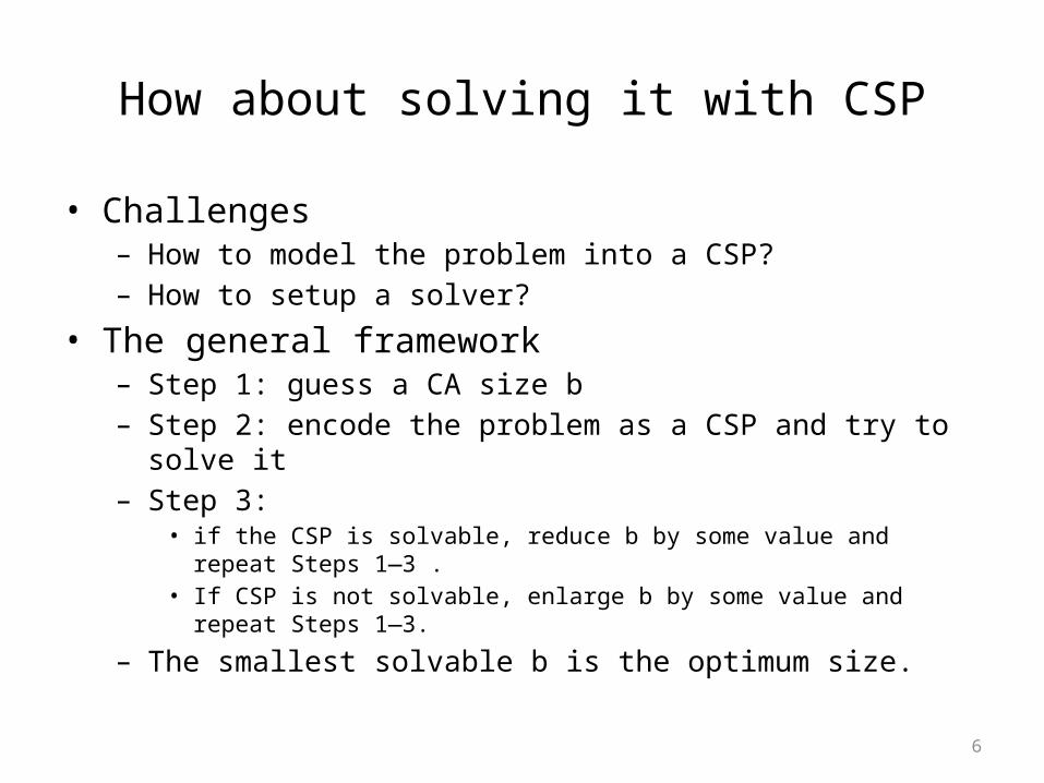
• Challenges– How to model the problem into a CSP?– How to setup a solver?

• The general framework– Step 1: guess a CA size b– Step 2: encode the problem as a CSP and try to solve it– Step 3:

• if the CSP is solvable, reduce b by some value and repeat Steps 1—3 . • If CSP is not solvable, enlarge b by some value and repeat Steps 1—3.

– The smallest solvable b is the optimum size.

How about solving it with CSP

7

Outline

• Introduction & Background• CSP model

– Naïve model, Alternative model, Integrated model

• Symmetry breaking• Solving the CSP

– Setting up the Ilog Solver, Experiment results

• SAT Model– Model, Experiment results

8

• Rows Each variable represents the value of one parameter in one vector: b×k matrix

– Example: k=5 (xi1..5), g=2 (0/1), t=3 (every combination of three parameters), b=5 (a total of 5 combinations/rows)

• How to express constraints?– Every subset of t parameters must be combined in all possible ways

A Naïve Matrix Model

x11 x12 x13 x14 x15x21 x22 x23 x24 x25x31 x32 x33 x34 x35x41 x42 x43 x44 x45x51 x52 x53 x54 x55

9

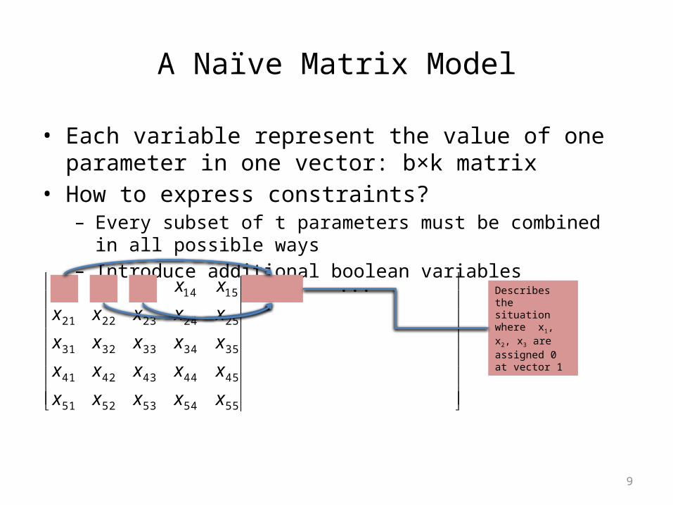
• Each variable represent the value of one parameter in one vector: b×k matrix

• How to express constraints?– Every subset of t parameters must be combined in all possible ways– Introduce additional boolean variables

A Naïve Matrix Model

x11 x12 x13 x14 x15x21 x22 x23 x24 x25x31 x32 x33 x34 x35x41 x42 x43 x44 x45x51 x52 x53 x54 x55

x1,123,000 ...

Describes the situation where x1, x2, x3 are assigned 0 at vector 1

10

• Each variable represent the value of one parameter in one vector: b×k matrix

• How to express constraints?– Every subset of t parameters must be combined in all possible ways

A Naïve Matrix Model

x11 x12 x13 x14 x15x21 x22 x23 x24 x25x31 x32 x33 x34 x35x41 x42 x43 x44 x45x51 x52 x53 x54 x55

x1,123,000 ...

x2,123,000 ...

x3,123,000 ...

x4,123,000 ...

x5,123,000 ...

1

11

• Each variable represent the value of one parameter in one vector: b×k matrix

• How to express constraints?– Every subset of t parameters must be combined in all possible ways– Question: How many columns are there for this example?

A Naïve Matrix Model

x11 x12 x13 x14 x15x21 x22 x23 x24 x25x31 x32 x33 x34 x35x41 x42 x43 x44 x45x51 x52 x53 x54 x55

x1,123,000 x1,123,001 ... x1,123,111 x1,124,000 ... x1,345,111x2,123,000 x2,123,001 ... x2,123,111 x2,124,000 ... x2,345,111x3,123,000 x3,123,001 ... x3,123,111 x3,124,000 ... x3,345,111x4,123,000 x4,123,001 ... x4,123,111 x4,124,000 ... x4,345,111x5,123,000 x5,123,001 ... x5,123,111 x5,124,000 ... x5,345,111

12

• Each variable represent the value of one parameter in one vector: b×k matrix

• How to express constraints?– Every subset of t parameters must be combined in all possible ways.– Express coverage constraints over columns (in general, columns)

– Clearly, this is not very efficient…

A Naïve Matrix Model

x11 x12 x13 x14 x15x21 x22 x23 x24 x25x31 x32 x33 x34 x35x41 x42 x43 x44 x45x51 x52 x53 x54 x55

x1,123,000 x1,123,001 ... x1,123,111 x1,124,000 ... x1,345,111x2,123,000 x2,123,001 ... x2,123,111 x2,124,000 ... x2,345,111x3,123,000 x3,123,001 ... x3,123,111 x3,124,000 ... x3,345,111x4,123,000 x4,123,001 ... x4,123,111 x4,124,000 ... x4,345,111x5,123,000 x5,123,001 ... x5,123,111 x5,124,000 ... x5,345,111

1

1

1

1

1

k

t

2t

13

• What did we learn from last model?– Setting up variables is simple and straightforward.– Expressing constraints is cumbersome and introduces numerous

assistant variables.

• Each variable represents a t-tuple in a vector (compound variable), domain is all possible values for the tuple.

Alternative Matrix Model

1,2,3 c1,1c2,1c3,1c4,1c5,1...

1,2,4 c1,2c2,2c3,2c4,2c5,2...

1,2,5 c1,3c2,3c3,3c4,3c5,3...

1,3,4 c1,4c2,4c3,4c4,4c5,4...

1,3,5 c1,5c2,5c3,5c4,5c5,5...

1,4,5 c1,6c2,6c3,6c4,6c5,6...

2,3,4 c1,7c2,7c3,7c4,7c5,7...

2,3,5 c1,8c2,8c3,8c4,8c5,8...

2,4,5 c1,9c2,9c3,9c4,9c5,9...

3,4,5 c1,10c2,10c3,10c4,10c5,10...

Domain of C1,1

Assignments for x1, x2, x3

0 0, 0, 0

1 0, 0, 1

2 0, 1, 0

3 0, 1, 1

4 1, 0, 0

5 1, 0, 1

6 1, 1, 0

7 1, 1, 1

14

1,2,3 0

0

1

2

3

4

5

6

7

7

1,2,4 0

1

0

2

3

4

5

7

6

7

1,2,5 0

1

1

3

2

5

4

6

6

7

1,3,4 0

1

2

0

3

4

7

5

6

7

1,3,5 0

1

3

1

2

5

6

4

6

7

1,4,5 0

3

1

1

2

5

6

6

4

7

2,3,4 0

1

2

4

7

0

3

5

6

7

2,3,5 0

1

3

5

6

1

2

4

6

7

2,4,5 0

3

1

5

6

1

2

6

4

7

3,4,5 0

3

5

1

6

1

6

2

4

7

• How to express constraints?– Now, each column represents all assignments for one specific tuple.– In each column, every number in the range 0 to 2t -1 should appear at

least once, and at most…– Question: How many times each number appears at most in a column?

– Enforcing such a global constraint on each column. ( constraints in total)

Alternative Matrix Model

k

t

15

x11 x12 x13 x14 x15x21 x22 x23 x24 x25x31 x32 x33 x34 x35x41 x42 x43 x44 x45x51 x52 x53 x54 x55

x1,123,000 x1,123,001 ... x1,123,111 x1,124,000 ... x1,345,111x2,123,000 x2,123,001 ... x2,123,111 x2,124,000 ... x2,345,111x3,123,000 x3,123,001 ... x3,123,111 x3,124,000 ... x3,345,111x4,123,000 x4,123,001 ... x4,123,111 x4,124,000 ... x4,345,111x5,123,000 x5,123,001 ... x5,123,111 x5,124,000 ... x5,345,111

• Improvement over the last model?

• Are we done?

Alternative Matrix Model

1,2,3 c1,1c2,1c3,1c4,1c5,1...

1,2,4 c1,2c2,2c3,2c4,2c5,2...

1,2,5 c1,3c2,3c3,3c4,3c5,3...

1,3,4 c1,4c2,4c3,4c4,4c5,4...

1,3,5 c1,5c2,5c3,5c4,5c5,5...

1,4,5 c1,6c2,6c3,6c4,6c5,6...

2,3,4 c1,7c2,7c3,7c4,7c5,7...

2,3,5 c1,8c2,8c3,8c4,8c5,8...

2,4,5 c1,9c2,9c3,9c4,9c5,9...

3,4,5 c1,10c2,10c3,10c4,10c5,10...

16

• Intersection Constraints– Values assigned to compound variables in the same vector should be

consistent.– In every row, if two variables share some positions, we impose a

binary constraint stating the allowed pairs of values.

Alternative Matrix Model

1,2,3 c1,1c2,1c3,1c4,1c5,1...

1,2,4 c1,2c2,2c3,2c4,2c5,2...

1,2,5 c1,3c2,3c3,3c4,3c5,3...

1,3,4 c1,4c2,4c3,4c4,4c5,4...

1,3,5 c1,5c2,5c3,5c4,5c5,5...

1,4,5 c1,6c2,6c3,6c4,6c5,6...

2,3,4 c1,7c2,7c3,7c4,7c5,7...

2,3,5 c1,8c2,8c3,8c4,8c5,8...

2,4,5 c1,9c2,9c3,9c4,9c5,9...

3,4,5 c1,10c2,10c3,10c4,10c5,10...

Allowed tuples

(0,0), (0,1), (1,0), (1,1), (2,2), (2,3), (3,2), (3,3), (4,4), (4,5), (5,4), (5,5), (6,6), (6,7), (7,6), (7,7)

17

• How many Intersection Constraints for each row?– For each compound variable, # of variables sharing ONE position is – # of variables sharing TWO positions– Continues until the case of sharing (t-1) positions

• For the CA(3, 5, 2) example– # of variables sharing ONE position is 3 – # of variables sharing TWO positions is 6– 10 variables in each row, (3+6)×10/2 = 45 constraints.

Alternative Matrix Model

1,2,3 1,2,4 1,2,5 1,3,4 1,3,5 1,4,5 2,3,4 2,3,5 2,4,5 3,4,5

t k t

t 1

t

2

k t

t 2

18

• How many Intersection Constraints for each row?– Reduction 1: the red constraint is redundant with the conjunction of

the two blue constraints and it can be removed.

– In general, constraints between variables that share fewer than t-1 positions in common, can be removed.

Alternative Matrix Model

1,2,3 1,2,4 1,2,5 1,3,4 1,3,5 1,4,5 2,3,4 2,3,5 2,4,5 3,4,5

1,2,3 1,2,4 1,2,5 1,3,4 1,3,5 1,4,5 2,3,4 2,3,5 2,4,5 3,4,5

1,2 1,41

19

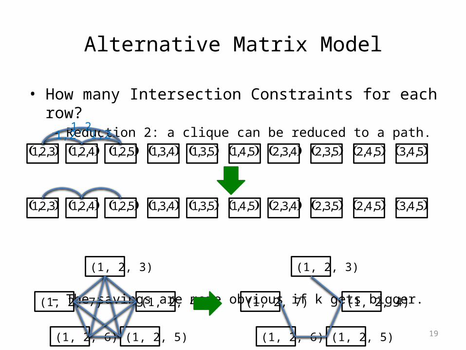
• How many Intersection Constraints for each row?– Reduction 2: a clique can be reduced to a path.

– The savings are more obvious if k gets bigger.

Alternative Matrix Model

1,2,3 1,2,4 1,2,5 1,3,4 1,3,5 1,4,5 2,3,4 2,3,5 2,4,5 3,4,5

1,2,3 1,2,4 1,2,5 1,3,4 1,3,5 1,4,5 2,3,4 2,3,5 2,4,5 3,4,5

(1, 2, 3)

(1, 2, 7) (1, 2, 4)

(1, 2, 6) (1, 2, 5)

(1, 2, 3)

(1, 2, 7) (1, 2, 4)

(1, 2, 6) (1, 2, 5)

1,21,2

1,2

20

• How many Intersection Constraints for each row?– Apply reduction 1: 45 30

Alternative Matrix Model

1,2,3 1,2,4 1,2,5 1,3,4 1,3,5 1,4,5 2,3,4 2,3,5 2,4,5 3,4,5

21

• How many Intersection Constraints for each row?– Apply reduction 1: 45 30

– Apply reduction 2: 30 20

Alternative Matrix Model

1,2,3 1,2,4 1,2,5 1,3,4 1,3,5 1,4,5 2,3,4 2,3,5 2,4,5 3,4,5

1,2,3 1,2,4 1,2,5 1,3,4 1,3,5 1,4,5 2,3,4 2,3,5 2,4,5 3,4,5

22

x11 x12 x13 x14 x15x21 x22 x23 x24 x25x31 x32 x33 x34 x35x41 x42 x43 x44 x45x51 x52 x53 x54 x55

x1,123,000 x1,123,001 ... x1,123,111 x1,124,000 ... x1,345,111x2,123,000 x2,123,001 ... x2,123,111 x2,124,000 ... x2,345,111x3,123,000 x3,123,001 ... x3,123,111 x3,124,000 ... x3,345,111x4,123,000 x4,123,001 ... x4,123,111 x4,124,000 ... x4,345,111x5,123,000 x5,123,001 ... x5,123,111 x5,124,000 ... x5,345,111

• Still, the # of intersection constraints is a problem – Why not apply the intersection constraints on the naïve model?

• To summarize so far– Naïve model suffers from # of additional variables.– The alternative model suffers from # of intersection constraints.– Can we combine the strengths together?

Alternative Matrix Model

Implicit connections

23

• Channeling constraint– explicitly express connections between compound variable and its

corresponding t variables in the naïve model.

– There are totally channeling constraints, each with arity t+1.– Enforcing GAC on them leads to assignment of x or domain reduce of c– Eliminate all intersection constraints.

Combining them together: an Integrated Model

x11 x12 x13 x14 x15x21 x22 x23 x24 x25x31 x32 x33 x34 x35x41 x42 x43 x44 x45x51 x52 x53 x54 x55

1,2,3 c1,1c2,1c3,1c4,1c5,1...

1,2,4 c1,2c2,2c3,2c4,2c5,2...

1,2,5 c1,3c2,3c3,3c4,3c5,3...

1,3,4 c1,4c2,4c3,4c4,4c5,4...

1,3,5 c1,5c2,5c3,5c4,5c5,5...

1,4,5 c1,6c2,6c3,6c4,6c5,6...

2,3,4 c1,7c2,7c3,7c4,7c5,7...

2,3,5 c1,8c2,8c3,8c4,8c5,8...

2,4,5 c1,9c2,9c3,9c4,9c5,9...

3,4,5 c1,10c2,10c3,10c4,10c5,10...

Extensionally (0,0,0,0), (1,0,0,1),(2,0,1,0),(3,0,1,1),(4,1,0,0),(5,1,0,1),(6,1,1,0),(7,1,1,1)

Intensionally C1,1=4x11+2x12+x13

k

t

b

24

Outline

• Introduction & Background• CSP model

– Naïve model, Alternative model, Integrated model

• Symmetry breaking• Solving the CSP

– Setting up the Ilog Solver, Experiment results

• SAT Model– Model, Experiment results

25

• CA has both row and column symmetries: any two cols/rows

• Another less obvious symmetry: value symmetry

• Size of the symmetry group: – So we must deal with them!

Symmetry

0 0 0 0 0

0 0 0 1 1

0 0 1 0 1

0 1 0 0 1

0 1 1 1 0

1 0 0 0 1

1 0 1 1 0

1 1 0 1 0

1 1 1 0 0

1 1 1 1 1

0 0 0 0 0

1 1 0 1 0

0 0 1 0 1

0 1 0 0 1

0 1 1 1 0

1 0 0 0 1

1 0 1 1 0

0 0 0 1 1

1 1 1 0 0

1 1 1 1 1

0 0 0 0 0

0 0 0 1 1

0 0 1 0 1

0 1 0 0 1

0 1 1 1 0

1 0 0 0 1

1 0 1 1 0

1 1 0 1 0

1 1 1 0 0

1 1 1 1 1

0 0 0 0 0

0 1 0 0 1

0 0 1 0 1

0 0 0 1 1

0 1 1 1 0

1 0 0 0 1

1 1 1 0 0

1 1 0 1 0

1 0 1 1 0

1 1 1 1 1

0 0 0 0 0

0 0 0 1 1

0 0 1 0 1

0 1 0 0 1

0 1 1 1 0

1 0 0 0 1

1 0 1 1 0

1 1 0 1 0

1 1 1 0 0

1 1 1 1 1

1 1 1 1 1

1 1 1 0 0

1 1 0 1 0

1 0 1 1 0

1 0 0 0 1

0 1 1 1 0

0 1 0 0 1

0 0 1 0 1

0 0 0 1 1

0 0 0 0 0

k!b! g! k

26

• For row and column symmetries– [Flener02] Theorem1: For a matrix model with row and column

symmetry in some 2-d matrix, each symmetry class of assignments has an element where both the rows and the columns of that matrix are lexicographically ordered.

– Naïve model: Impose lexicographical ordering constraints on both rows and columns of the matrix

– Alternative model: rows are the same, columns are not as powerful, but can be help

– Integrated model: can apply lexicographical ordering on either original or alternative matrix, but not both.

Symmetry Breaking

0 0 0 0 0

0 0 0 1 1

0 0 1 0 1

0 1 0 0 1

0 1 1 1 0

1 0 0 0 1

1 0 1 1 0

1 1 0 1 0

1 1 1 0 0

1 1 1 1 1

27

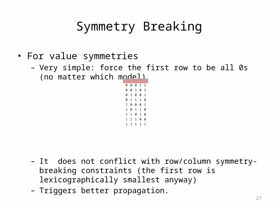
• For value symmetries– Very simple: force the first row to be all 0s (no matter which model)

– It does not conflict with row/column symmetry-breaking constraints (the first row is lexicographically smallest anyway)

– Triggers better propagation.

Symmetry Breaking

0 0 0 0 0

0 0 0 1 1

0 0 1 0 1

0 1 0 0 1

0 1 1 1 0

1 0 0 0 1

1 0 1 1 0

1 1 0 1 0

1 1 1 0 0

1 1 1 1 1

28

Outline

• Introduction & Background• CSP model

– Naïve model, Alternative model, Integrated model

• Symmetry breaking• Solving the CSP

– Setting up the Ilog Solver, Experiment results

• SAT Model– Model, Experiment results

29

• Use ILOG Solver 6.0• Use compound variables as search variables

– Coverage constraints expressed over compound variables

• Variable and value ordering– Values assigned in ascending order– Labeling variables by column (coverage constraints are on columns)– Lexicographical ordering within each column

• Symmetry-breaking constraints (as shown before)• Channeling constraints

– Extensional: GAC– Intensional: bounds consistency– Same for domain of binary alphabet: each value is a bound. However,

solver may run faster on bounds consistency

Setting up the solver

30

• Results for CA(3, k, 2)

– For alternative model, both with all/minimal intersection constraints– For integrated model, channeling constraints expressed both

extensionally (GAC) and intensionally (bounds consistency).– * indicates finding optimal size of b.

Experiment results

31

• Results for CA(3, k, 2)

– For integrated model, enforcing intensional constraints is cheaper than enforcing extensional constraints.

Experiment results

32

• Results for CA(3, k, 2)

– Integrated model is better than alternative model– For k=12, integrated model has 220 channeling constraints, while

alternative model has 594 non-redundant intersection constraints.

Experiment results

33

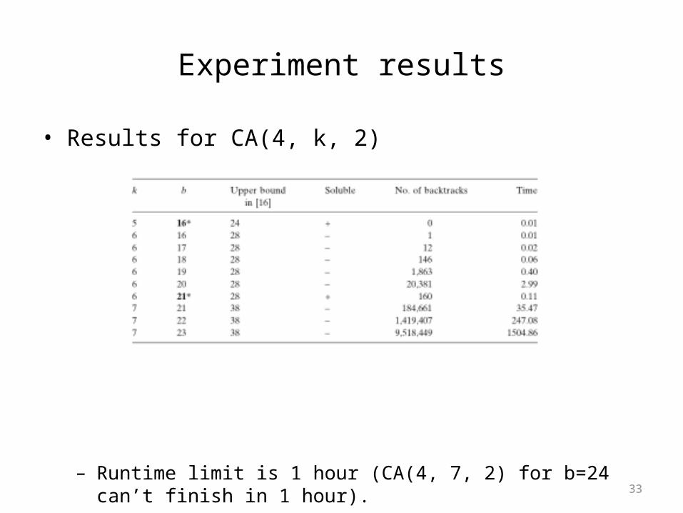
• Results for CA(4, k, 2)

– Runtime limit is 1 hour (CA(4, 7, 2) for b=24 can’t finish in 1 hour).

Experiment results

34

Outline

• Introduction & Background• CSP model

– Naïve model, Alternative model, Integrated model

• Symmetry breaking• Solving the CSP

– Setting up the Ilog Solver, Experiment results

• SAT Model– Model, Experiment results

35

• Encoding the problem into CNF SAT (Example CA(2, 3, 2))

– Still have two matrices: original and alternative– Create a Boolean variable for EACH value of EACH variable.

Local search model with SAT

x11 x12 x13x21 x22 x23x31 x32 x33... ... ...

m11,0 m11,1 m12,0 m12,1 m13,0 m13,1

m21,0 m21,1 m22,0 m22,1 m23,0 m23,1

m31,0 m31,1 m32,0 m32,1 m33,0 m33,1

... ... ... ... ... ...

c11 c12 c13c21 c22 c23c31 c32 c33... ... ...

a11,0 a11,1 a11,2 a11,3 a12,0 a12,1 a12,2 a12,3 a13,0 a13,1 a13,2 a13,3a21,0 a21,1 a21,2 a21,3 a22,0 a22,1 a22,2 a22,3 a23,0 a23,1 a23,2 a23,3a31,0 a31,1 a31,2 a31,3 a32,0 a32,1 a32,2 a32,3 a33,0 a33,1 a33,2 a33,3... ... ... ... ... ... ... ... ... ... ... ...

(1,2), (2,3), (1,3)

36

• Encoding the problem into CNF SAT

Local search model with SAT

x11 x12 x13x21 x22 x23x31 x32 x33... ... ...

m11,0 m11,1 m12,0 m12,1 m13,0 m13,1

m21,0 m21,1 m22,0 m22,1 m23,0 m23,1

m31,0 m31,1 m32,0 m32,1 m33,0 m33,1

... ... ... ... ... ...

(1)

x

mijx

(2)

m ijx m ijx'

(1,2), (2,3), (1,3)

c11 c12 c13c21 c22 c23c31 c32 c33... ... ...

a11,0 a11,1 a11,2 a11,3 a12,0 a12,1 a12,2 a12,3 a13,0 a13,1 a13,2 a13,3a21,0 a21,1 a21,2 a21,3 a22,0 a22,1 a22,2 a22,3 a23,0 a23,1 a23,2 a23,3a31,0 a31,1 a31,2 a31,3 a32,0 a32,1 a32,2 a32,3 a33,0 a33,1 a33,2 a33,3... ... ... ... ... ... ... ... ... ... ... ...

m11,0 m11,1

m 11,0 m 11,1

37

• Encoding the problem into CNF SAT

Local search model with SAT

x11 x12 x13x21 x22 x23x31 x32 x33... ... ...

m11,0 m11,1 m12,0 m12,1 m13,0 m13,1

m21,0 m21,1 m22,0 m22,1 m23,0 m23,1

m31,0 m31,1 m32,0 m32,1 m33,0 m33,1

... ... ... ... ... ...

(1)

(2)

m ijx m ijx'

(3)

y

aij 'y

(4)

a ij 'y a ij 'y'

(1,2), (2,3), (1,3)

c11 c12 c13c21 c22 c23c31 c32 c33... ... ...

a11,0 a11,1 a11,2 a11,3 a12,0 a12,1 a12,2 a12,3 a13,0 a13,1 a13,2 a13,3a21,0 a21,1 a21,2 a21,3 a22,0 a22,1 a22,2 a22,3 a23,0 a23,1 a23,2 a23,3a31,0 a31,1 a31,2 a31,3 a32,0 a32,1 a32,2 a32,3 a33,0 a33,1 a33,2 a33,3... ... ... ... ... ... ... ... ... ... ... ...

m11,0 m11,1

m 11,0 m 11,1

a11,0 a11,1 a11,2 a11,3

(a 11,0 a 11,1) (a 11,0 a 11,2) (a 11,0 a 11,3) (a 11,1 a 11,2) (a 11,1 a 11,3) (a 11,2 a 11,3)

x

mijx

38

• Encoding the problem into CNF SAT

Local search model with SAT

x11 x12 x13x21 x22 x23x31 x32 x33... ... ...

m11,0 m11,1 m12,0 m12,1 m13,0 m13,1

m21,0 m21,1 m22,0 m22,1 m23,0 m23,1

m31,0 m31,1 m32,0 m32,1 m33,0 m33,1

... ... ... ... ... ...

(1)

x

mijx

(2)

m ijx m ijx'

(3)

y

aij 'y

(4)

a ij 'y a ij 'y'

(5)

iaij 'y

(1,2), (2,3), (1,3)

c11 c12 c13c21 c22 c23c31 c32 c33... ... ...

a11,0 a11,1 a11,2 a11,3 a12,0 a12,1 a12,2 a12,3 a13,0 a13,1 a13,2 a13,3a21,0 a21,1 a21,2 a21,3 a22,0 a22,1 a22,2 a22,3 a23,0 a23,1 a23,2 a23,3a31,0 a31,1 a31,2 a31,3 a32,0 a32,1 a32,2 a32,3 a33,0 a33,1 a33,2 a33,3... ... ... ... ... ... ... ... ... ... ... ...

a11,0 a11,1 a11,2 a11,3

(a 11,0 a 11,1) (a 11,0 a 11,2) (a 11,0 a 11,3) (a 11,1 a 11,2) (a 11,1 a 11,3) (a 11,2 a 11,3)

m11,0 m11,1

m 11,0 m 11,1

a11,0 a21,0 a31,0

39

• Encoding the problem into CNF SAT

Local search model with SAT

x11 x12 x13x21 x22 x23x31 x32 x33... ... ...

m11,0 m11,1 m12,0 m12,1 m13,0 m13,1

m21,0 m21,1 m22,0 m22,1 m23,0 m23,1

m31,0 m31,1 m32,0 m32,1 m33,0 m33,1

... ... ... ... ... ...

(1)

x

mijx

(2)

m ijx m ijx'

(3)

y

aij 'y

(4)

a ij 'y a ij 'y'

(5)

iaij 'y

(6)

a ij 'y mijx

(1,2), (2,3), (1,3)

c11 c12 c13c21 c22 c23c31 c32 c33... ... ...

a11,0 a11,1 a11,2 a11,3 a12,0 a12,1 a12,2 a12,3 a13,0 a13,1 a13,2 a13,3a21,0 a21,1 a21,2 a21,3 a22,0 a22,1 a22,2 a22,3 a23,0 a23,1 a23,2 a23,3a31,0 a31,1 a31,2 a31,3 a32,0 a32,1 a32,2 a32,3 a33,0 a33,1 a33,2 a33,3... ... ... ... ... ... ... ... ... ... ... ...

a11,0 a11,1 a11,2 a11,3

(a 11,0 a 11,1) (a 11,0 a 11,2) (a 11,0 a 11,3) (a 11,1 a 11,2) (a 11,1 a 11,3) (a 11,2 a 11,3)

m11,0 m11,1

m 11,0 m 11,1

a11,0 a21,0 a31,0

(a 11,0 m11,0) (a 11,0 m12,0)

40

• Encoding the problem into CNF SAT

Local search model with SAT

x11 x12 x13x21 x22 x23x31 x32 x33... ... ...

m11,0 m11,1 m12,0 m12,1 m13,0 m13,1

m21,0 m21,1 m22,0 m22,1 m23,0 m23,1

m31,0 m31,1 m32,0 m32,1 m33,0 m33,1

... ... ... ... ... ...

(1)

x

mijx

(2)

m ijx m ijx'

(3)

y

aij 'y

(4)

a ij 'y a ij 'y'

(5)

iaij 'y

(6)

a ij 'y mijx

(1,2), (2,3), (1,3)

c11 c12 c13c21 c22 c23c31 c32 c33... ... ...

a11,0 a11,1 a11,2 a11,3 a12,0 a12,1 a12,2 a12,3 a13,0 a13,1 a13,2 a13,3a21,0 a21,1 a21,2 a21,3 a22,0 a22,1 a22,2 a22,3 a23,0 a23,1 a23,2 a23,3a31,0 a31,1 a31,2 a31,3 a32,0 a32,1 a32,2 a32,3 a33,0 a33,1 a33,2 a33,3... ... ... ... ... ... ... ... ... ... ... ...

a11,0 a11,1 a11,2 a11,3

(a 11,0 a 11,1) (a 11,0 a 11,2) (a 11,0 a 11,3) (a 11,1 a 11,2) (a 11,1 a 11,3) (a 11,2 a 11,3)

m11,0 m11,1

m 11,0 m 11,1

a11,0 a21,0 a31,0

(a 11,0 m11,0) (a 11,0 m12,0)

41

• Encoding the problem into CNF SAT

Local search model with SAT

x11 x12 x13x21 x22 x23x31 x32 x33... ... ...

m11,0 m11,1 m12,0 m12,1 m13,0 m13,1

m21,0 m21,1 m22,0 m22,1 m23,0 m23,1

m31,0 m31,1 m32,0 m32,1 m33,0 m33,1

... ... ... ... ... ...

(1)

x

mijx

(2)

m ijx m ijx'

(3)

y

aij 'y

(4)

a ij 'y a ij 'y'

(5)

iaij 'y

(6)

a ij 'y mijx

(1,2), (2,3), (1,3)

c11 c12 c13c21 c22 c23c31 c32 c33... ... ...

a11,0 a11,1 a11,2 a11,3 a12,0 a12,1 a12,2 a12,3 a13,0 a13,1 a13,2 a13,3a21,0 a21,1 a21,2 a21,3 a22,0 a22,1 a22,2 a22,3 a23,0 a23,1 a23,2 a23,3a31,0 a31,1 a31,2 a31,3 a32,0 a32,1 a32,2 a32,3 a33,0 a33,1 a33,2 a33,3... ... ... ... ... ... ... ... ... ... ... ...

a11,0 a11,1 a11,2 a11,3

(a 11,0 a 11,1) (a 11,0 a 11,2) (a 11,0 a 11,3) (a 11,1 a 11,2) (a 11,1 a 11,3) (a 11,2 a 11,3)

m11,0 m11,1

m 11,0 m 11,1

a11,0 a21,0 a31,0

(a 11,0 m11,0) (a 11,0 m12,0)

42

• SAT local search algorithm– First, randomly assign all boolean variables.– Select a violated clause, flip the value of one variable in it (satisfy the

clause, but may cause others to violate).– Repeat until timeout or satisfied.

• Variable selection heuristic– With probability p, randomly select a variable. (noise, set to .2, .3, .4)– With 1-p, pick variable with min score

– Break ties by selecting the variable that was least recently flipped.– Freebie move: if there are multiple variables such that flipping them

would not create new unsat clauses (score=0), break ties randomly.

Setting up the solver

# of unsatisfied clauses results from flipping v

total # of flips in the past on all variables other than vScore =

Smallest negative

effect Prefer variables that have

fewest flips

43

Results for local search model: CA(2, k, g)

*bold denotes best results.

HW: HWFSAT (2006)HR: Hartmann & Raskin 2004CK: Chateaunef & Kreher 2002MS: Meagher & Stevens 2005NU: Nurmela 2004

44

• CA(3, k, g)

• CA(4, k, g)

Results for local search model

Better than the other 2

In fact, they are optimal, but do we

know they are optimal?

45

• Modeling CA problem into CSP– Naïve model– Alternative model– Integrated model

• Local search with SAT– Handles larger problems– Trade scalability with completeness– Combining results with CSP results may be valuable

Summary

46

• Page 203, first formula:• Page 203, fifth line from bottom: variables • Page 212, 20th line from top:

Small Typos in Paper

xrl p

(xri,xrj ,xrl )

iaij 'y

47

• References– Hnich et al. ‘06: Constraints models for the covering test problems– Flener et al. ‘02: Breaking row and column symmetry in matrix models– Frisch et al. ‘02: Global constraints for lexicographical orderings– Gent et al. ‘95: Unsatisfied variables in local search– Hartman et al. ‘04:Problems and algorithms for covering arrays– Chateauneuf et al. ‘02: On the state of strength-three covering arrays– Meagher et al. ‘05: Group construction of covering arrays– Nurmela et al. ‘04: Upper bounds for covering arrays by Tabu search

• The switches and light bulbs shown on first slide is a real game– http://www.devicedaily.com/gadgets/awesome-wooden-switch-and-b

ulb-game-resurrects-1960s-idea.html

Literature

48

Discussion