constraint-based design of parallel kinematic xy flexure...
TRANSCRIPT

Awtar, ASME MD-06-1015 1
Constraint-based Design of Parallel Kinematic XY Flexure Mechanisms
Shorya Awtar1 Precision Engineering Research Group Massachusetts Institute of Technology, Cambridge MA 518-577-5500, [email protected] Alexander H. Slocum Professor of Mechanical Engineering, Precision Engineering Research Group Massachusetts Institute of Technology, Cambridge MA 617-253-0012, [email protected]
Abstract
This paper presents parallel kinematic XY flexure mechanism designs based on systematic
constraint patterns that allow large ranges of motion without causing over-constraint or
significant error motions. Key performance characteristics of XY mechanisms such as mobility,
cross-axis coupling, parasitic errors, actuator isolation, drive stiffness, lost motion, and geometric
sensitivity are discussed. The standard double parallelogram flexure module is used as a
constraint building-block and its non-linear force-displacement characteristics are employed in
analytically predicting the performance characteristics of two proposed XY flexure mechanism
designs. Fundamental performance tradeoffs, including those resulting from the non-linear load-
stiffening and elastokinematic effects, in flexure mechanisms are highlighted. Comparisons
between closed-form linear and non-linear analyses are presented to emphasize the inadequacy
of the former. It is shown that geometric symmetry in the constraint arrangement relaxes some of
the design tradeoffs, resulting in improved performance. The non-linear analytical predictions
are validated by means of computational FEA and experimental measurements.
Keywords: Constraint-based Flexure Design, XY Flexure, Non-linear Flexure Analysis, Flexure
Performance Characteristics, Flexure Design Tradeoffs, Center of Stiffness
1 Corresponding Author

Awtar, ASME MD-06-1015 2
1. Introduction and Background
Compact XY flexure stages that provide large range of motion are desirable in several
applications such as semiconductor mask and wafer alignments [1], scanning interferometry and
atomic force microscopy [2-3], micromanipulation and microassembly [4], high-density memory
storage [5], and MEMS sensors and actuators [6-7]. Despite numerous designs that exist in the
technical literature [1, 8-10], flexure stages generally lack in motion range. Challenges in the
design of large range mechanisms arise from the basic tradeoff between Degrees of Freedom
(DOF) and Degrees of Constraint (DOC) in flexures [11]. As constraint elements, flexures pose a
compromise between the motion range along DOF and the stiffness and error motions along
DOC. These tradeoffs are further pronounced due to the non-linear load-stiffening and
elastokinematic effects in distributed-compliance flexure mechanisms, which are nevertheless
desirable due to elastic-averaging [11-12]. Load-stiffening refers to the increase in stiffness in
the presence of loads, and elastokinematic effect characterizes the specific displacement
component that has a kinematic dependence on other displacements as well as an elastic
dependence on loads. While deterministic mathematical techniques for flexure design exist [13-
14], these are best suited for shape and size synthesis. Constraint-based design has generally
proven to be effective in flexure mechanism topology generation [15]. Accordingly, several new
parallel kinematic XY flexure mechanisms based on a systematic and symmetric arrangement of
common flexure modules, in a fashion that does not over-constrain the primary motions, have
been proposed [11, 16]. Some representative designs, the underlying constraint pattern, key
performance characteristics, and design challenges and tradeoffs are presented in this paper.
A closed-form non-linear analysis is employed to predict the performance of the proposed XY
mechanisms, which utilize the standard double parallelogram flexure module. Although the
presented analysis is valid for any general shape of the constituent beams in these modules,
uniform-thickness simple beams are assumed for the purpose of illustration. Non-linearities
associated with the beam curvature, which can be modeled using elliptical integrals [17] or the
pseudo-rigid body method [18], have been neglected since deflections considered here are an
order less the beam length. However, load-stiffening and elastokinematic non-linearities
resulting from the deformed-state force equilibrium conditions can play a significant role in
determining the influence of loads and displacements in one direction on the stiffness and error
motion properties of other directions. Since these non-linearities can arise for displacements of

Awtar, ASME MD-06-1015 3
the order of the beam thickness and significantly influence the performance of a flexure
mechanism, they cannot be ignored. Existing treatments of load-stiffening and elastokinematic
effects in beams are either too complex for closed-form analysis [19] or case-specific [20]. Due
to their assumed lumped-compliance topology, pseudo-rigid body models do not capture
elastokinematic effects. Therefore, a generalized analytical formulation based on simple yet
accurate approximations for the non-linear force-displacement relationships of the beam flexure
[11-12] is used here.
A realistic performance prediction, not possible using a linear analysis, is thus obtained without
the need for iterative or numerical methods. The parametric nature of these results offers several
insights into XY flexure mechanism design, particularly in terms of performance characteristics
and compromises therein. The presented analyses also provide a mathematical verification of the
design axiom that geometric symmetry in mechanism design yields improved performance. To
verify the analytical predictions, an experimental setup has been designed that accommodates
multiple sensors and actuators to reliably characterize one of the proposed XY flexure
mechanism designs.
2. XY Mechanism Topology Design
There are two kinds of design configurations for multi-DOF mechanisms – serial and parallel.
Serial designs present a stacked assembly of several single-DOF stages and incorporate moving
actuators and cables, which can be detrimental for precision and dynamic performance. Parallel
designs, which are considered here, are usually compact and allow ground mounting of actuators.
While the generic performance characteristics of flexures such as mobility, error motions and
stiffness variations have been defined in the prior literature [12], the specific desirable attributes
of a parallel kinematic XY flexure mechanism and associated challenges are listed here.
1. The primary objective of the design is to achieve large ranges of motion along the desired
directions X and Y, and an obvious limitation comes from material failure criteria. For a given
maximum stress level, high compliance in the directions of primary motion or DOF increases the
range of motion. However, in designs with out-of-plane constraints, this conflicts with the need
to maintain high stiffness and small error motions in the out-of-plane directions, thus making
planer designs preferable.
Awtar, ASME MD-06-1015 4
2. In an XY mechanism, the motion stage yaw is often undesirable. Given this requirement, the
motion stage yaw may be rejected passively or actively. While both options have respective
advantages, fewer actuators make the former favorable due to reduced design complexity and
potentially better motion range. Thus, the mechanism has to be designed such that the rotation of
the motion stage, being a parasitic error motion, is inherently constrained. This error motion
may be further attenuated by exploiting the Center of Stiffness (COS) concept to appropriately
place the actuators, as explained in the following section.
3. Minimal cross-axis coupling between the X and Y degrees of freedom is an important
performance requirement, especially in applications where end-point feedback is not feasible or
the two axes are not actively controlled. Cross-axis coupling refers to any motion along the Y
direction in response to an actuation along the X direction, and vice versa. In the absence of end-
point feedback, it necessitates an additional calibration step to determine the transformation
matrix between the actuator coordinates and the motion stage coordinates. In unactuated or
under-actuated systems, cross-axis coupling can lead to undesirable internal resonances.
4. An important challenge in parallel mechanism design for positioning is that of integrating the
ground-mounted actuators with the motion stage. Linear displacement or force source actuators
typically do not tolerate transverse loads and displacements. Therefore, the point of actuation on
the flexure mechanism must be such that it only moves along the direction of actuation and has
minimal transverse motions in response to any actuator in the system. Eliminating transverse
motion at the point of actuation, is termed as actuator isolation, and is generally difficult to
achieve due to the parallel geometry.
5. In the absence of adequate actuator isolation, the actuators have to be connected to the point
of actuation by means of a decoupler, which ideally transmits axial force without any loss in
motion and absorbs any transverse motions without generating transverse loads. However, a
flexure-based decoupler, which is desirable to maintain precision, is subject to its own tradeoffs.
Increasing its motion range and compliance in the transverse direction results in lost motion
between the actuator and motion stage, affecting precision, and loss in stiffness along its axial
direction. The latter contributes to drive stiffness, which is the overall stiffness between the point
of actuation and the motion stage, and influences the dynamic performance of the motion system.

Awtar, ASME MD-06-1015 5
6. Low thermal and manufacturing sensitivities are important performance parameters for
precision flexure mechanisms in general. Both these factors, being strongly dependent on the
mechanism’s geometry, may be improved by careful use of reversal and symmetry.
Because of the tradeoff between quality of DOF and DOC, all these performance measures
including parasitic errors, cross-axis coupling, actuator isolation, lost motion and drive stiffness,
deteriorate with increasing range of motion, as shall be shown quantitatively in the subsequent
sections. Depending upon the application, these collectively restrict the range of a parallel
kinematic mechanism to a level much smaller than what is allowed by material limits. While
geometric symmetry plays an important role in improving performance, it can overconstrain the
primary directions resulting in a significantly reduced range, if implemented inappropriately.
MotionStage
IntermediateStage 1
IntermediateStage 2
Flexure B
Flexure C
Flex
ure
A
Flexure DGround:Fixed Stage
X
Y
Z
Fig.1 Proposed Constraint Arrangement for XY Flexure Mechanisms
Fig. 1 illustrates the proposed constraint arrangement that can help achieve the above-listed
desirable attributes in XY mechanisms. The constraint arrangement includes four basic rigid
stages: Ground, Motion Stage, and intermediate Stages 1 and 2. Stage 1 is connected to ground
by means of flexure module A, which only allows relative X translation; the Motion Stage is
connected to Stage 1 via flexure module B, which only allows relative Y translation; the Motion
Stage is connected to Stage 2 via flexure module C, which only allows a relative X translation;
and finally, Stage 2 is connected to Ground by means of flexure module D, which only allows
relative Y translation. Thus, in any deformed configuration of the mechanism, Stage 1 will
always have only an X displacement with respect to Ground while Stage 2 will have only a Y

Awtar, ASME MD-06-1015 6
displacement. Furthermore, the Motion Stage inherits the X displacement of Stage 1 and the Y
displacement of Stage 2, thus acquiring two translational degrees of freedom that are mutually
independent. Since the Y and X displacements of the Motion Stage do not influence Stage 1 and
Stage 2, respectively, these are ideal locations for applying the actuation loads, obviating the
need for decouplers.
In an ideal scenario where the flexure modules A, B, C and D are perfect constraints, this
arrangement would yield a flawless design. However, due to the inherent imperfection in
flexures, the actual resulting designs are expected to deviate slightly from ideal behavior. Any
approximately linear motion flexure module can be used as the building-blocks A, B, C and D.
Fig. 2 presents a design based on the double parallelogram flexure module. Although simple
beams are illustrated, other beam shapes may be employed as well. The double parallelogram
flexure offers large range, good rotational stiffness, no purely kinematic parasitic errors, and
excellent thermal stability.
Ground
MotionStage
Stage 1
Stage 2
ao
bo
my
fy
Xo
Yo
2w1
2w2
fx
mx
X
Y
1
4
3
2
sx
sy
Fig.2 XY Flexure Mechanism Design 1

Awtar, ASME MD-06-1015 7
Without causing overconstraint, this design is further enhanced by making use of symmetry,
which involves adding intermediate Stages 3 and 4, and repeating the constraint arrangement
described earlier. The resulting design, illustrated in Fig. 3, is expected to exhibit superior
performance. Since the relative rotation in the double parallelogram module is elastic and
elastokinematic in nature, motion stage rotation in both these mechanisms may be mitigated by
appropriately locating the actuation forces on the intermediate stages [12]. The axes of X and Y
actuation that minimize the motion stage yaw are referred to as the Center of Stiffness axes.
1
6
5
4
3
2
7
8
ao
ro
bo
fx
mx
fymy
Stage 1
Ground
GroundGround
Ground
Stage 2
Stage 3
Stage 4
Xo
Yo
MotionStage
2w2
2w1
X
Y
so
Fig.3 XY Flexure Mechanism Design 2
At this point, it is interesting to highlight the inadequacy of the traditional mobility criteria in
determining the DOF of flexure mechanisms. Gruebler’s criterion predicts a DOF of 1 for
Design 1, and –1 for Design 2. In other words, Design 1 should only allow a single independent
Awtar, ASME MD-06-1015 8
actuation, while Design 2 should be immobile due to over-constraint. Both these predictions are
incorrect because the geometric constraint arrangement in each of these cases results in
redundant constraints. In rigid-link mechanisms, geometric imperfections arising from
manufacturing and assembly, can cause otherwise redundant constraints to become independent,
a possibility that is accurately captured by Gruebler’s criterion. However, in flexure mechanisms,
particularly distributed-compliance topologies, elastic averaging plays an important role in
ensuring that redundant constraints remain unaffected despite small geometric variations. Elastic
averaging is a consequence of finite stiffness along the constraint directions in flexures. Thus,
while the lack of ideal constraint behavior in flexures results in performance compromises on
one hand, it is also responsible for allowing special geometries in mechanism topology design.
Several other XY designs with different space utilization, choice of building-blocks, and levels
of symmetry can be generated using the proposed constraint arrangement [16]. The performance
of any resulting mechanism depends on the constraint characteristics of the individual building-
blocks and the geometry of the constraint arrangement, as shall be shown analytically in the
following sections.
3. Performance Prediction of Proposed XY Mechanisms
fλ
pλ2w1 2w2
mλ
xλ
yλθλ
SecondaryStage
PrimaryStage
Ground
X
Y
Ground
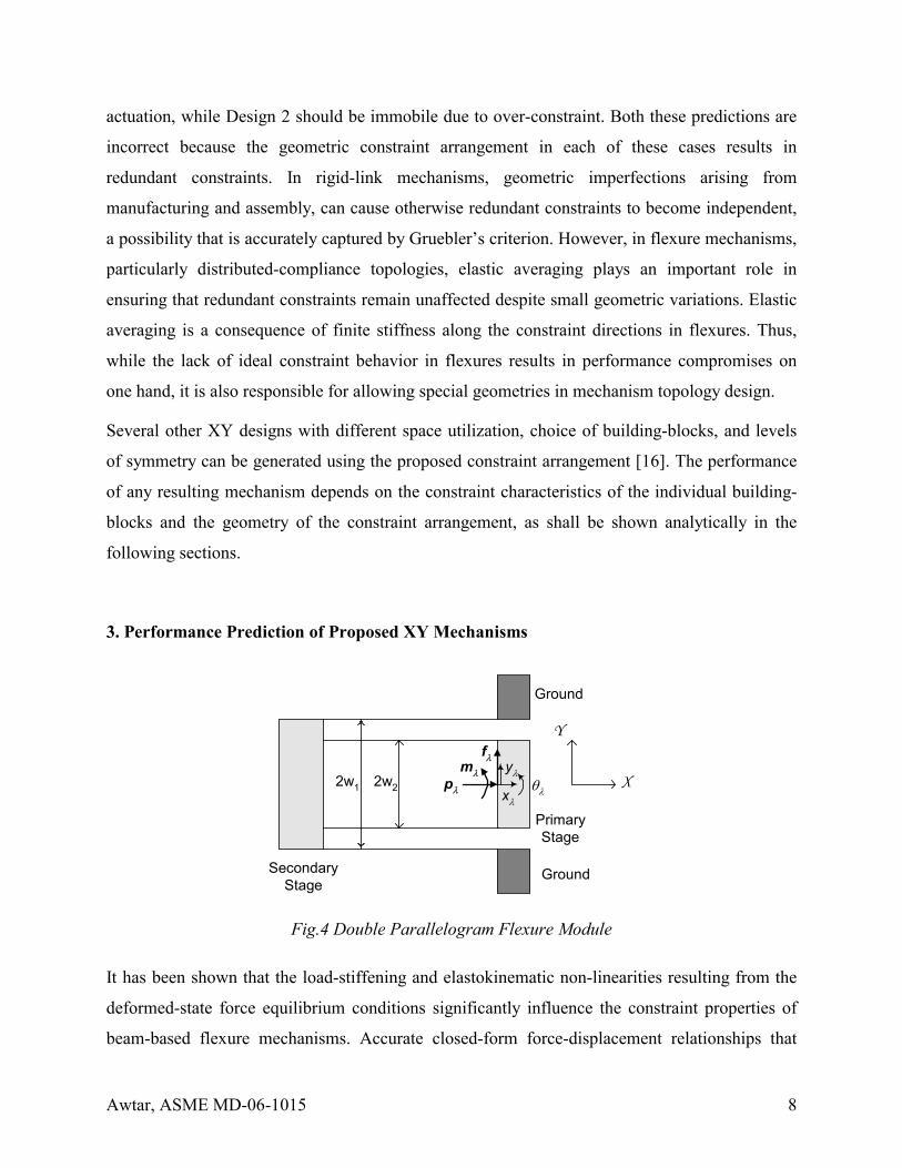
Fig.4 Double Parallelogram Flexure Module
It has been shown that the load-stiffening and elastokinematic non-linearities resulting from the
deformed-state force equilibrium conditions significantly influence the constraint properties of
beam-based flexure mechanisms. Accurate closed-form force-displacement relationships that

Awtar, ASME MD-06-1015 9
incorporate these non-linearities have been derived for the double parallelogram flexure [12],
and shall be used in the analysis of the proposed XY mechanisms. With reference to Fig. 4, the
linear and non-linear force-displacement results for the double parallelogram flexure are
reproduced below.
Linear Analysis:
where 2
2 2
12w d 2 2
2 1 212 22w d1 2
1a
1w d
1d
0y2w www w
x 0
00
λ λ
λ λ
λ λ
θ
⎡ ⎤⎡ ⎤ ⎡ ⎤⎢ ⎥⎢ ⎥ ⎢ ⎥= ⎢ ⎥⎢ ⎥ ⎢ ⎥ +⎢ ⎥⎢ ⎥ ⎢ ⎥⎣ ⎦ ⎣ ⎦⎣ ⎦
fmp
(1)
Non-Linear Analysis:
( ) ( )2 2
4ay2a e
λλ
λ
≈−fp
( ) ( ) ( ) ( )
( ) ( ) ( )
2
221
2
222
1 1 r 1 2c h2w d 2a e 2a e2a e
1 1 r 2c h2w d 2a e2a e
λ λ λλ λ λ
λ λλ
λ λλ λ
λλ
θ⎞⎛ ⎡ ⎤⎞⎛
≈ + − − + −⎟⎜ ⎢ ⎥⎟⎜ ⎟⎜ ⎟ − +− ⎢ ⎥⎝ ⎠⎣ ⎦⎝ ⎠⎞⎛ ⎡ ⎤
+ + − +⎟⎜ ⎢ ⎥⎜ ⎟ ++ ⎣ ⎦⎝ ⎠
f f pm pp pp
f fm ppp
(2)
( ) ( )( )
2 2 22
2
r 2a e 8aei 1 y r eix yd 4a d 2 2 a
λλ λλ λ λ λ
⎡ ⎤+ − ⎡ ⎤⎞⎛⎣ ⎦= + ≈ + −⎜ ⎟⎢ ⎥⎝ ⎠⎣ ⎦
pp p p
In the above expressions, fλ, mλ, pλ, yλ, θλ, and xλ represent normalized transverse force,
moment, axial force, transverse displacement, rotation, and axial displacement, respectively, for
a given double parallelogram flexure module. All displacements and length parameters are
normalized by the beam length L, forces by E'Izz/L2, and moments by E'Izz/L. E' denotes Young’s
modulus for plane stress, and plate modulus for plane strain. The coefficients a, c, e, h, i and r
are all non-dimensional numbers that are characteristic of the beam shape, and assume the
following values for a simple beam with uniform thickness: a=12, c=−6, e=1.2, h=−0.1,
i=−0.6, and r =1/700. Although simple beams are used for illustration, these force-displacement
results and all the subsequent derivations are valid for any general beam shape.
The primary and secondary stages, along with ground, are assumed rigid in arriving at the above
results. Therefore, the normalized elastic axial stiffness of the double parallelogram module is

Awtar, ASME MD-06-1015 10
simply given by the elastic axial stiffness of the constituent beams, d. For a simple beam, d
assumes a value of 12/t2, where t is the normalized beam thickness. If the dimensions of the
primary, secondary or ground stages are such that they cannot be assumed perfectly rigid,
additional elastic stiffness or compliance contributions should be included in the above
expressions. This primarily affects the axial stiffness of the double parallelogram module.
In analyzing the two proposed XY mechanism designs, force equilibrium is applied in the
deformed configuration of the mechanism to capture the relevant non-linearities. Ground,
Motion Stage and the Intermediate Stages are all assumed perfectly rigid. For typical
dimensions, the transverse elastic stiffness, a, of the beam is several orders of magnitude smaller
than its axial elastic stiffness, d, and may generally be neglected in comparison. Being small,
rotations may also be neglected wherever their contribution is relatively insignificant. All non-
dimensional quantities are represented by lower case alphabets throughout this paper.
3.1 XY Mechanism Design 1
XY Mechanism Design 1 is shown in a deformed configuration in Fig. 5, where the rigid frames
including Ground, Motion Stage and the two intermediate stages are represented by solid lines,
and the compliance of the double parallelograms is denoted by the small circles. The planer
rotations of the Motion Stage and the two intermediate stages are exaggerated for the purpose of
illustration. Free Body Diagrams of the individual stages are also included. The relative
displacements of each constituent flexure module are given by,
λ λθ yλ xλ
1 1θ 1 o 1x a θ+ y1
2 2θ 2 o 2y b θ− 2x
3 s 1θ θ− ( ) ( )s o s 1 o 1y a y bθ θ− − + s 1x x−
4 s 2θ θ+ ( ) ( )2 o 2 s o sx a x bθ θ− − + s 2y y−

Awtar, ASME MD-06-1015 11
θ1
θ2
(x1,y1 )
(xs ,ys )p2
1
4
3
2
(x2 ,y2 )
θs
f4m4
X
Y
p3
f3m3
p4
myfy
Stage 2
mx
fx
p1
f1m1
f2
m2
Stage 1
p2f2
m2
p3
f3m3
MotionStage
Ground
Fig.5 XY Mechanism 1 in a Deformed Configuration
There are three internal forces per flexure module and three displacements per stage, resulting in
21 unknowns. The three force-displacement relations per flexure module, given by (1), and three
force-equilibrium relations per stage provide 21 equations. Since the internal forces are not of
interest, instead of solving these equations explicitly, energy methods are employed to efficiently
obtain the following summarized force-displacement results for the linear case.
1 2 2 3 sx
1 3 3 2 sy
2 3 4 5 1x
2 3 4 5 2y
3 2 5 5 4 s
k 0 k k k x0 k k k k yk k k 0 kk k 0 k kk k k k k0
θθθ
− − −⎡ ⎤ ⎧ ⎫⎧ ⎫⎢ ⎥ ⎪ ⎪⎪ ⎪⎢ ⎥ ⎪ ⎪⎪ ⎪⎪ ⎪ ⎪ ⎪⎢ ⎥= − −⎨ ⎬ ⎨ ⎬⎢ ⎥⎪ ⎪ ⎪ ⎪− −⎢ ⎥⎪ ⎪ ⎪ ⎪⎢ ⎥− − −⎪ ⎪ ⎪ ⎪⎩ ⎭ ⎣ ⎦ ⎩ ⎭
ffmm
where ( )( )
( ) ( )( ) ( )
11
2 o 21
3 o 22 2 2
4 o o o o1
5 o o o o2
k 2ak a ak a b
k a a b a b a 2w dk a b a a a b
=
= − +
= − −
= + − − +
= − −
(3)
The Motion Stage rotation can be obtained by inverting the above stiffness matrix.
( )( ) ( )s x x o o y y o o4
1 a b a bk
θ = − + + + +m f m f
This expression shows that the motion stage rotation can be made identically zero if mx=
fx(ao+bo) and my= −fy(ao+bo), which implies that the COS axes for the Motion Stage with

Awtar, ASME MD-06-1015 12
respect to the X and Y actuation forces is given by Xo and Yo, shown in Fig. 2. Not being
intuitively obvious, this is useful information if Motion Stage yaw is to be minimized passively.
With this choice of actuation force locations, the remaining displacements can be calculated from
the matrix expression (3).
( ) ; ; =
( ) ; = ;
( ) ( )
( ) ( )
2x o x x
s y 1 s 22
2y y yo
s x 1 2 s2
o o o1 x y2 2
o o o2 x y2 2
2a 1x x x x2a 16w d 2d 2d
2b 1y y y y2a 16w d 2d 2d
1 2a 4b 1 2b8w d 8w d
1 2a 1 4a 2b8w d 8w d
θ
θ
+= + = +
−= + = +
− − −= − −
+ + += − −
f f ff
f f ff
f f
f f
(4)
Since the linear analysis captures only elastic effects, it should be recognized that these results
are valid only for small loads and displacements. Nevertheless, they provide valuable design help
not only in determining the actuator locations but also in selecting the geometric parameters ao
and bo so as to minimize cross-axis coupling and intermediate stage rotations. In this case, the
above results indicate that the dimension ao should be kept as small as possible and bo should be
chosen to be 1/2.
To accurately predict the elastokinematic effects that become prominent with increasing loads
and displacements, we proceed to perform a non-linear analysis. The 21 equations, including the
non-linear force displacement relations (2) for the double parallelogram, are explicitly solved
using the symbolic computation tool MAPLE™. Taking advantage of the normalized
framework, higher order small terms are dropped at appropriate steps in the analysis, and the
following force-displacement results for the mechanism are obtained.
( )( )( ) ( )
22o
s x y o 1 o 2 o s2 2 2y
1 a 1 2ax 8a 8a a a b4a e w d
θ θ θ⎡ ⎤+
= + − + +⎢ ⎥− ⎣ ⎦f f
f (5)
( )( )( ) ( )
22o
s y x o 1 o 2 o s2 2 2x
1 a 1 2by 8a 8a b b a4a e w d
θ θ θ⎡ ⎤−
= + + + +⎢ ⎥− ⎣ ⎦f f
f (6)
( ) ( ) ; 2 2
2 11 s x 1 y
y ra 2 ei 1 x ra 2 ei 1x x y4a 2d 4a 2d
⎡ ⎤ ⎡ ⎤− −= + + = +⎢ ⎥ ⎢ ⎥
⎣ ⎦ ⎣ ⎦f f (7)
Awtar, ASME MD-06-1015 13
( ) 1 ( ) 1 ; =2d 2d
2 21 2
2 s y 2 xx ra 2 ei y ra 2 eiy y x
4a 4a⎡ ⎤ ⎡ ⎤− −
= + + +⎢ ⎥ ⎢ ⎥⎣ ⎦ ⎣ ⎦
f f (8)
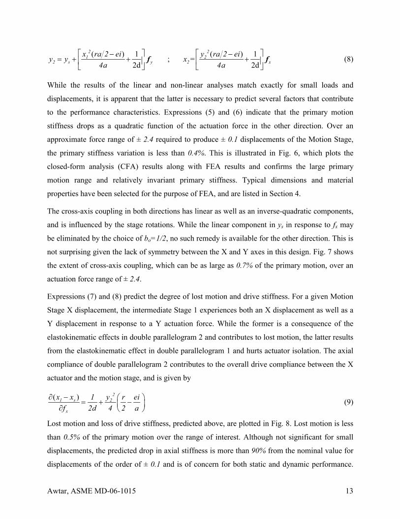
While the results of the linear and non-linear analyses match exactly for small loads and
displacements, it is apparent that the latter is necessary to predict several factors that contribute
to the performance characteristics. Expressions (5) and (6) indicate that the primary motion
stiffness drops as a quadratic function of the actuation force in the other direction. Over an
approximate force range of ± 2.4 required to produce ± 0.1 displacements of the Motion Stage,
the primary stiffness variation is less than 0.4%. This is illustrated in Fig. 6, which plots the
closed-form analysis (CFA) results along with FEA results and confirms the large primary
motion range and relatively invariant primary stiffness. Typical dimensions and material
properties have been selected for the purpose of FEA, and are listed in Section 4.
The cross-axis coupling in both directions has linear as well as an inverse-quadratic components,
and is influenced by the stage rotations. While the linear component in ys in response to fx may
be eliminated by the choice of bo=1/2, no such remedy is available for the other direction. This is
not surprising given the lack of symmetry between the X and Y axes in this design. Fig. 7 shows
the extent of cross-axis coupling, which can be as large as 0.7% of the primary motion, over an
actuation force range of ± 2.4.
Expressions (7) and (8) predict the degree of lost motion and drive stiffness. For a given Motion
Stage X displacement, the intermediate Stage 1 experiences both an X displacement as well as a
Y displacement in response to a Y actuation force. While the former is a consequence of the
elastokinematic effects in double parallelogram 2 and contributes to lost motion, the latter results
from the elastokinematic effect in double parallelogram 1 and hurts actuator isolation. The axial
compliance of double parallelogram 2 contributes to the overall drive compliance between the X
actuator and the motion stage, and is given by
( ) 21 s 2
x
x x 1 y r eif 2d 4 2 a
∂ − ⎞⎛= + −⎜ ⎟∂ ⎝ ⎠ (9)
Lost motion and loss of drive stiffness, predicted above, are plotted in Fig. 8. Lost motion is less
than 0.5% of the primary motion over the range of interest. Although not significant for small
displacements, the predicted drop in axial stiffness is more than 90% from the nominal value for
displacements of the order of ± 0.1 and is of concern for both static and dynamic performance.

Awtar, ASME MD-06-1015 14
To restrict the loss in drive stiffness to less than 25%, the motion range of this design has to be
limited to ± 0.0125.
Actuator isolation is determined by the amount of Y displacement at the point of X force
application. If the X force is applied along the COS axis, Xo, the extent of actuator isolation is
given by (y1−sxθ1), which is plotted in Fig. 9. The lack of actuator isolation for the Y actuator
can be as large as 1.5% of the primary motion for the force ranges of interest.
-2 -1 0 1 2-0.15
-0.1
-0.05
0
0.05
0.1
0.15
Y Force ( fy )
y s
fx = -2.4, 0, 2.4
-2 -1 0 1 2-6
-4
-2
0
2
4
6x 10
-4
Y Force ( fy )
x s - x s( f
y=0 )
fx= -1.6
fx=1.6
fx= 0
Fig.6 Primary Motion: : CFA (–) and FEA (o) Fig.7 Cross-Axis Error Motion: CFA (–) and FEA (o)
-2 -1 0 1 2-3
-2
-1
0
1
2
3x 10
-4
Y Force ( fy )
x s- x1
fx= 0.8
fx= - 0.8 fx= 0
fx= 1.6
fx= -1.6
-2 -1 0 1 2
-2
-1
0
1
2
x 10-4
Y Force ( fy )
y 1 - s x θ
1
fx= -1.6
fx= - 0.8
fx= 0.8 fx= 1.6
fx= 0
Fig.8 Lost Motion / Drive Stiffness: CFA (–) and FEA (o) Fig.9 Actuator Isolation: CFA (–) and FEA (o)
Awtar, ASME MD-06-1015 15
For simplicity, Motion Stage rotation is expressed here for two special cases.
( ) ( )
( ) ( )
for
for
2 2s x o x o x x o x o x x y y2 2
2 2s y o y o y y o y o y y x x2 2
1 32a a b rd 2 a b 064a w d
1 32a a b rd 2 a b 064a w d
θ
θ
⎡ ⎤= − − + − − = =⎣ ⎦
⎡ ⎤= + + + + + = =⎣ ⎦
m f f m f f f f m
m f f m f f f f m (10)
For small loads and displacements, these expressions yield COS axes identical to those predicted
by the linear analysis. With no independent moments, and actuation forces acting along axes Xo
and Yo, the Motion Stage rotation reduces to
( )( )
( ) ( ) +
o o 3 2 2 3s x x y x y y2 2 2 2
x y
x y2 2 2 2 2 2
2 x y
a brw 64a 2rd
1 4 2ah cea d w w 32a rd
θ+
⎡ ⎤= ⋅ ⋅ + − −⎣ ⎦+ +
⎧ ⎫⋅ − − ⋅⎨ ⎬
+ +⎩ ⎭
f f f f f ff f
f ff f
(11)
This shows that while it is possible to entirely eliminate the linear, or purely elastic, component
of the Motion Stage rotation by selecting the force locations, the same is not true for the non-
linear elastokinematic components because the COS shifts with increasing loads. Since the
applied moments cannot be controlled independent of the forces, the mechanism’s geometry
plays an important role in the effectiveness of this passive yaw minimization method. Motion
Stage rotation is plotted against the X and Y actuation forces in Fig. 10, which not only illustrate
the inadequacy of the linear analysis but also provide an idea of the range beyond which the non-
linear effects become important. For the chosen mechanism dimensions, the maximum rotation is
approximately 40 µrad over a motion range of ± 0.1. To ensure a motion stage rotation of less
than 5 µrad, the motion range of this design is restricted to ± 0.05.
Sensitivity of the Motion Stage yaw to the location of force application may also be analytically
determined to simulate assembly and manufacturing tolerances that can cause an offset between
the COS axis and the actual actuation axis. If ex represents this offset, then the Motion Stage yaw
is given by the following expression in the absence of any Y actuation.
( )2
3 xs o o x x x2 2
1 32a er a b 2e f f64a w d
θ⎡ ⎤
= + + +⎢ ⎥⎣ ⎦
(12)

Awtar, ASME MD-06-1015 16
-2 -1 0 1 2-5
-4
-3
-2
-1
0
1
2
3
4
5x 10⁻⁵
X Force ( fx)
Mot
ion
Sta
ge R
otat
ion
( θs )
fy=2.4
fy=1.2
fy= -2.4
fy= -1.2
fy= 0
Fig.10 Motion Stage Rotation: CFA (Contour), CFA (–) and FEA (o)
Result (12) is corroborated by FEA in Fig. 11, where fx is kept fixed at 0.25. This picture will
obviously change with increasing loads and in the presence of fy.
-2 -1 0 1 2-6
-4
-2
0
2
4
6
8x 10
-5
X Force Location ( ex )
Stag
e R
otat
ions θ1 θs
θ2
fx = 0.25
Fig.11 Moment Sensitivity and COS for the Stages with respect X Force: CFA (–) and FEA (o)
With the actuation forces applied along the COS of the Motion Stage, the intermediate stage
rotations are calculated using the non-linear analysis for specific cases.
fy fx
θs

Awtar, ASME MD-06-1015 17
( ) ( )
( ) ( ) ( )
for
for
2 22 3x
1 o o x o o x y2 2 2 2x
2 31 o y o o y x2 2 2
y
1 rd 16a 16a 1 2a 4b rd a b 064a w d rd 32a
1 16a 2b 1 rd a b 1 04w d rd 32a
θ
θ
⎞⎛ + ⎡ ⎤= − − − + + =⎟⎜ ⎣ ⎦+⎝ ⎠
⎡ ⎤= − − − + =⎣ ⎦+
f f f ff
f f ff
(13)
( ) ( ) ( )
( ) ( )
for
for
2 32 o x o o x y2 2 2
x
2 2y 2 3
2 o o y o o y x2 2 2 2y
1 16a 1 2a rd a b 1 04w d rd 32a
rd 16a1 16a 1 2b 4a rd a b 064a w d rd 32a
θ
θ
⎡ ⎤= − + − − + =⎣ ⎦+
⎞⎛ +⎡ ⎤= − + + − + =⎟⎜ ⎣ ⎦⎜ ⎟+⎝ ⎠
f f ff
ff f f
f
(14)
The intermediate stage rotations are obviously large and have a dominant linear component, with
the non-linear contribution two orders of magnitude smaller. The dependence of Stage 1 rotation
on fy is clearly attenuated with the choice of bo=1/2. This is not true of Stage 2, which therefore
sees a higher maximum rotation. The difference between the rotations of the two intermediate
stages is due to the lack of symmetry in this design. These rotations are plotted in Figures 12 and
13 for various loading conditions.
If the application so demands, the actuation forces may be alternatively applied along the COS
axes of Stage 1 or Stage 2, but this obviously affects the Motion Stage rotation. Both the linear as
well as non-linear analyses reveal that the COS for Stage 1 with respect to X actuation force is
located at a distance (1+2bo+4ao)/6 from the nominal location, and with respect to the Y
actuation force is located at (1−2ao−4bo)/2, which actually corresponds to the Yo axis for bo=0.5.
Similarly, the COS of Stage 2 with respect to the Y actuation force is located at a distance
(1−2ao−4bo)/6 from the nominal location, and with respect to X actuation force is located at
(1+2bo+4ao)/2. A force location that results in a positive moment, following the convention of
Fig. 2, is considered positive and vice versa. These results are also precisely validated by FEA in
Fig. 11.
Thus, it is seen that XY Mechanism Design 1 offers a good range of primary motions, although
other performance attributes such as cross-axis coupling, parasitic rotations, actuator isolation
and drive stiffness deteriorate with increasing primary motion. Improvements in performance
may be achieved by applying the actuation forces along the COS axes and choosing geometric
parameters judiciously. Given its compact geometry, this design may be quite suitable for several
applications.

Awtar, ASME MD-06-1015 18
-2 -1 0 1 2
-1
-0.5
0
0.5
1
x 10-4
Y Force ( fy )
θ 1
fx= 0
fx= -1.6
fx= - 0.8
fx= 0.8
fx= 1.6
-2 -1 0 1 2
-5
-2.5
0
2.5
5x 10
-4
Y Force ( fy )
θ 2
fx= 0
fx= -1.6
fx= - 0.8
fx= 0.8
fx= 1.6
Fig.12 Stage 1 Rotation: CFA (–) and FEA (o) Fig.13 Stage 2 Rotation: CFA (–) and FEA (o)
3.2 XY Mechanism Design 2
Fig. 14 illustrates the XY Mechanism Design 2 in a deformed configuration, along with the FBD
and displacements of the stages. As in the previous case, stage rotations are exaggerated. The
relative displacements for the individual double parallelogram flexure modules, represented by
the small circles, are given by
λ λθ yλ xλ
1 1θ 1 o 1x a θ− 1y
2 2θ 2 o 2y a θ+ 2x−
3 s 1θ θ+ ( ) ( )s o s 1 o 1y r y bθ θ− − − s 1x x−
4 s 2θ θ+ ( ) ( )s o s 2 o 2x r x bθ θ− + + + s 2y y−
5 s 7θ θ− ( ) ( )s o s 7 o 7y r y bθ θ− + + − s 7x x− +
6 s 8θ θ− ( ) ( )s o s 8 o 8x r x bθ θ− − + s 8y y− +
7 7θ 7 o 7x a θ− 7y−
8 8θ 8 o 8y a θ− 8x
There are 3 unknown displacements per stage and 3 unknown internal forces per flexure module,
resulting in 39 unknowns. The 3 force equilibrium relations per stage and 3 constitutive relations
per flexure module provide 39 equations necessary to solve these unknowns.

Awtar, ASME MD-06-1015 19
fx
mx
fy
my
(xs,ys )
θ1
θs
θ2
θ8
θ7
m1
1
6
5
4
3
2
78
f1
p1
m3
f3p3
m6
f6
p6
m8
f8
p8
m7
f7
p7
m5
f5
p5
m4
f4
p4
m2
f2
p2
X
Y
Stage 1
MotionStage
Stage 4
Stage 3
Stage 2
(x1,y1 )
(x2 ,y2 )
(x7 ,y7 )
(x8 ,y8 ) Ground
Ground
Ground
Ground
Fig.14 XY Mechanism 2 in a Deformed Configuration
As earlier, a linear analysis is performed first, using the linear constitutive relations (1) for the
modules, which yields the following force-displacement results for the overall mechanism.
1 2 3 2 3 s x
1 3 2 3 2 s y
2 3 4 5 1 x
3 2 4 5 2 y
2 3 4 5 7
3 2 4 5 8
5 5 5 5 6 s
k 0 k k k k 0 x0 k k k k k 0 yk k k 0 0 0 kk k 0 k 0 0 kk k 0 0 k 0 k 0k k 0 0 0 k k 00 0 k k k k k 0
θθθθθ
⎡ ⎤ ⎧ ⎫ ⎧ ⎫⎢ ⎥ ⎪ ⎪ ⎪ ⎪− −⎢ ⎥ ⎪ ⎪ ⎪ ⎪⎢ ⎥ ⎪ ⎪− − ⎪ ⎪−
⎪ ⎪ ⎪ ⎪⎢ ⎥− = −⎨ ⎬ ⎨ ⎬⎢ ⎥⎪ ⎪ ⎪ ⎪⎢ ⎥− ⎪ ⎪ ⎪ ⎪⎢ ⎥⎪ ⎪ ⎪ ⎪⎢ ⎥⎪ ⎪ ⎪ ⎪⎢ ⎥− − ⎩ ⎭⎣ ⎦ ⎩ ⎭
ffmm where,
( )( )
( ) ( )
( ) ( )
( ) ( )
11
2 o 21
3 o 22 2 2
4 o o o o21 1
5 o o o2 221 1
6 o o o2 2
k 4ak a ak a b
k a a b a b a 2w d
k ab r ar w d
k 4ar r 4 ar w d
=
= − +
= − −
= + − − +
= + + +
= + + +
These equations may be further solved to determine the displacements explicitly.

Awtar, ASME MD-06-1015 20
( )( ) ; ; o yx o x x xs 1 s 7 s2 2
2b 12a 1 3x x x x x4a 16dw 16dw 4d 4d
−+= − − = + = −
mf m f f
( )( ) ; ; y o y y yo xs 2 s 8 s2 2
2a 1 32b 1y y y y y4a 16dw 16dw 4d 4d
+−= + − = + = −f m f fm
; ; ; y yx x2 8 1 7x x y y
4d 4d 4d 4d= = = =
f ff f (15)
( )( ) o y yo x x1 2 2 2 2
2b 12a 1 516dw 16dw 8dw 8dw
θ−+
= − − −f mf m ;
( )( ) o y yo x x7 2 2 2 2
2b 12a 116dw 16dw 8dw 8dw
θ−+
= − + +f mf m
( ) ( )o y yo x x2 2 2 2 2
2a 1 52b 116dw 16dw 8dw 8dw
θ+ −
= + − −f mf m ;
( ) ( )o y yo x x8 2 2 2 2
2a 1 2b 116dw 16dw 8dw 8dw
θ+ −
= + + +f mf m
yxs 2 24dw 4dw
θ = +mm
Once again, several interesting observations can be made from this preliminary analysis. Motion
Stage rotation is predicted to be identically zero in the absence of any applied moments,
irrespective of the geometric dimensions. This implies that the COS axes of the motion stage
correspond to Xo and Yo, which coincide with the nominal actuation locations, as shown in Fig.
3. Furthermore, the elastic contribution in the error motions can be minimized by choosing the
smallest possible ao, and bo=1/2. With this choice of design parameters, the above results also
show that the rotations of intermediate stages 1 and 3 are not affected by the Y actuation force,
and those of intermediate stages 2 and 4 are not affected by X actuation force. Also, these results
claim that there should be a perfect decoupling between the two axes.
A more accurate prediction of the mechanism behavior is obtained by solving the system
equations using the nonlinear force-displacement relations (2) for the modules. By neglecting
insignificant terms at each step in the derivation, the following displacement results are obtained
using MAPLE™.
( )( ) ( )
2 2 3 2 22 yx x
s 2 2 2 2 2 2y y
64a y e i 64ax4a 4a64a 3e 64a 3e
+= ≈
− −
ff ff f
(16)

Awtar, ASME MD-06-1015 21
( )( )( )
( )
2 2 22 2yx x 2
1 2 2 2 2 2 2y y
2 2x x 2
2 2 2y
192a 11e64a y r ei 1x4a 4 2 2 a d64a 3e 64a 3e
64a 3 y ei 14a 4 2a d64a 3e
−⎧ ⎫⎞⎛= + − +⎨ ⎬⎜ ⎟− −⎝ ⎠⎩ ⎭
⎞⎛≈ + − + ⎟⎜− ⎝ ⎠
ff ff f
f ff
(17)
( )( )( )
( )
2 2 22 2yx x 2
7 2 2 2 2 2 2y y
2 2x x 2
2 2 2y
64a e64a y r ei 1x4a 4 2 2 a d64a 3e 64a 3e
64a y ei 14a 4 2a d64a 3e
−⎧ ⎫⎞⎛= − − +⎨ ⎬⎜ ⎟− −⎝ ⎠⎩ ⎭
⎞⎛≈ − − + ⎟⎜− ⎝ ⎠
ff ff f
f ff
(18)
2x 2
2y r ei 1x
4 2 2 a d⎧ ⎫⎞⎛= − +⎨ ⎬⎜ ⎟
⎝ ⎠⎩ ⎭
f (19) 2
x 28
y r ei 1x4 2 2 a d
⎧ ⎫⎞⎛= − +⎨ ⎬⎜ ⎟⎝ ⎠⎩ ⎭
f (20)
( )( ) ( )
2 2 3 2 21 xy y
s 2 2 2 2 2 2x x
64a x e i 64ay4a 4a64a 3e 64a 3e
+= ≈
− −
ff ff f
(21)
( )( )( )
( )
2 2 22 2xy y 1
2 2 2 2 2 2 2x x
2 2y y 1
2 2 2x
192a 11e64a x r ei 1y4a 4 2 2 a d64a 3e 64a 3e
364a x ei 14a 4 2a d64a 3e
−⎧ ⎫⎞⎛= + − +⎨ ⎬⎜ ⎟− −⎝ ⎠⎩ ⎭
⎞⎛≈ + − + ⎟⎜− ⎝ ⎠
ff ff f
f ff
(22)
( )( )( )
( )
2 2 22 2xy y 1
8 2 2 2 2 2 2x x
2 2y y 1
2 2 2x
64a e64a x r ei 1y4a 4 2 2 a d64a 3e 64a 3e
64a x ei 14a 4 2a d64a 3e
−⎧ ⎫⎞⎛= − − +⎨ ⎬⎜ ⎟− −⎝ ⎠⎩ ⎭
⎞⎛≈ − − + ⎟⎜− ⎝ ⎠
ff ff f
f ff
(23)
2y 1
1x r ei 1y
4 2 2 a d⎧ ⎫⎞⎛= − +⎨ ⎬⎜ ⎟
⎝ ⎠⎩ ⎭
f (24)
2y 1
7x r ei 1y
4 2 2 a d⎧ ⎫⎞⎛= − +⎨ ⎬⎜ ⎟
⎝ ⎠⎩ ⎭
f (25)
As in the previous case, the non-linear analysis predicts several important factors that determine
the mechanism's performance characteristics that are not captured by the linear analysis. Due to
twice the number of double parallelogram modules, the normalized force required to generate a
nominal primary motion of ± 0.1 in this case is approximately 4.8, twice that for Design 1. Fig.
15 confirms the large primary motion, which follows a predominantly linear behavior and is free

Awtar, ASME MD-06-1015 22
of any over-constraining effects. It may be noticed in expression (16) that the primary stiffness in
the X direction changes with the Y force. This is expected because upon the application of a
positive Y force, flexure modules 4, 6 and 7 experience a compressive axial force, while module
1 sees a tensile axial force. Irrespective of whether the axial force is tensile or compressive, the
transverse stiffness of all these modules drops resulting in an overall reduction in the primary
motion stiffness. However, over the range of the applied forces, the drop in primary motion
stiffness is less than 1.2%, which is barely noticeable in FEA results and experimental
measurements plotted in Fig. 15. The geometric dimensions and material properties of the
mechanism used in the FEA and experimental testing are listed in the following section.
Expressions (16) and (21) show that the linear elastic component of the cross-axis coupling in
this case is entirely eliminated. Any contributions from the applied moments and stage rotations
are also cancelled out due to symmetry. However, there remains a quadratic elastokinematic
component comparable to that in Design 1, and is plotted in Fig. 16. The worst-case cross-axis
error is on the order of 1% of the primary motion. Lost motion and change in drive stiffness are
given by expressions (17) and (21). Being approximately two orders smaller than the next larger
terms, the higher order terms in these expressions may be neglected. As in Design 1, the drive
stiffness between the actuator and Motion Stage reduces with increasing primary motions owing
to the double parallelogram characteristics. These predictions are validated in Fig. 17 by means
of FEA and experimental measurements. Maximum lost motion is approximately 1% of the
primary motion, while the drop in drive stiffness is the same as in the previous case. Clearly,
these attributes are not significantly affected by the overall mechanism’s geometric layout, and
are strongly dependent on the characteristics of the constraint building-blocks.
The degree of actuator isolation is given by the amount of X displacement at the point of Y
actuation on Stage 2. This is given by (x2−soθ2) and is comprised of linear and quadratic
components. The quadratic component results from the elastokinematic effect in double
parallelogram flexure module 2, derived in expression (19), in response to an X actuation force
and Y primary motion. Actuator isolation is plotted in Fig. 18 and is shown to be up to 0.6% of
primary motion, which is similar to the previous design.

Awtar, ASME MD-06-1015 23
-3 -2 -1 0 1 2 3-0.08
-0.06
-0.04
-0.02
0
0.02
0.04
0.06
0.08
Y Force ( fy )
y s
fx = - 3.214, 0, 3.214
-3 -2 -1 0 1 2 3-4
-3
-2
-1
0
1
2
3
4x 10⁻⁴
Y Force ( fy )
x s - x s( f
y=0 )
fx = 3.214
fx = 0
fx = 1.607
fx = - 1.607
fx = - 3.214
Fig.15 Primary Motion: CFA (–), FEA (o), Exp (*) Fig.16 Cross-axis Error Motion:
CFA (–), FEA (o), Exp (*)
-0.5 0 0.5 1 1.5 2 2.5 3 3.5-0.5
0
0.5
1
1.5
2
2.5
3
3.5
4
4.5x 10⁻⁴
Y Force ( fy )
x s - x 1
x1 = - 0.06, - 0.045, - 0.03, - 0.015, 0
-3 -2 -1 0 1 2 3-3
-2
-1
0
1
2
3x 10⁻⁴
Y Force ( fy )
x 2 - s o θ
2
fx = 3.214
fx = 1.607
fx = 0
fx = - 1.607
fx = - 3.214
Fig.17 Lost Motion / Drive Stiffness:
CFA (–), FEA (o), Exp (*) Fig.18 Actuator Isolation: CFA (–), FEA (o), Exp (*)
Next, the stage rotations can also be analytically calculated and the non-linear results are
presented here for some specific cases. Motion Stage rotation is given by
( ) ( ) for and for
2 2 2 2x y
s x y y s y x x2 2 2 2
64a rd 64a rd0 0
256a w d 256a w dθ θ
+ += = = = = =
f fm f m m f m (26)

Awtar, ASME MD-06-1015 24
This validates the inference drawn from the linear analysis regarding the COS location.
Remarkably, this choice of COS axes which corresponds to mx= my= 0 not only eliminates the
linear elastic component in the Motion Stage rotation, but also some of the non-linear terms. The
overall dependence of Motion Stage rotation on the X and Y actuation forces is presented in Fig.
19. From the large flat area in the central region of the 3D contour, it is apparent that the Motion
Stage rotation has been considerably suppressed despite the elastokinematic errors of the double
parallelogram flexure module. In fact, it is possible to keep the motion stage rotation less than 5
µrad over the entire motion range of ± 0.1 in both directions. Given the considerably small
magnitude of the Motion Stage rotation, the accuracy of both the closed-form as well as finite
element analyses is expected to be limited. Nevertheless, Fig. 19 indicates a fair agreement
between the two analysis methods, in terms of magnitudes and trends. Experimental
measurements of the stage rotation yielded a random variation within ± 10 µrad, which is very
likely due to extraneous factors.
-3 -2 -1 0 1 2 3-4
-3
-2
-1
0
1
2
3x 10
-6
Y Force ( fy )
Mot
ion
Sta
ge R
otat
ion
( θs )
fx = 3.214
fx = 1.607
fx = 0
fx = - 1.607
fx = - 3.214
Fig.19 Motion Stage Rotation: CFA (Contour), CFA (Lines) and FEA (Marks)
Expression (26) also provides a quantitative assessment of the sensitivity of the stage rotation
with respect to offsets ex and ey in the actuation axis, by setting mx=fx ex and my=fy ey. This is two
times better than the previous design for small loads, and four times better for higher loads. The
specific case of fx = 0 and fy = 3.214 is plotted in Fig. 20, along with FEA results.
fx fy
θs
o fx = 3.214 fx = 1.607 fx = 0 fx = -1.607
x fx = -3.214

Awtar, ASME MD-06-1015 25
-1 -0.5 0 0.5 1-3
-2
-1
0
1
2
3
4
5x 10⁻⁴
Y Force Location ( ey )
Stag
e R
otat
ions
θ1 θs
θ2
fy = 3.214
Fig.20 Moment Sensitivity and COS for the Stages with respect Y Force: CFA (–) and FEA (o)
Finally, we present the rotation of the intermediate stages assuming general loads but specific
cases, to avoid complex expressions. For y y0= =f m ,
( )2 2 22 2x x x o xx
1 2 2 2 2x
rd 32a 1 2a 320a64a rd128a rd 256a w d
θ⎡ ⎤− + + −⎞⎛ + ⎣ ⎦= ⎟⎜ +⎝ ⎠
f m f mff
( ).2 2x o xx
2 2 2 2x
a b 0 5 a64a rd128a rd 4aw d
θ− −⎡ ⎤⎞⎛ + ⎣ ⎦= ⎟⎜ +⎝ ⎠
f mff
(27)
( )2 2 22 2x x x o xx
7 2 2 2 2x
rd 32a 1 2a 64a64a rd128a rd 256a w d
θ⎡ ⎤+ + +⎞⎛ + ⎣ ⎦= ⎟⎜ +⎝ ⎠
f m f mff
( ).2 2x o xx
8 2 2 2x
a b 0 5 a64a rd128a rd 4aw d
θ− +⎡ ⎤⎞⎛ + ⎣ ⎦= ⎟⎜ +⎝ ⎠
f mff
These expressions provide the COS of the intermediate stages with respect to X actuation.
Similarly, the intermediate stage rotations for x x0= =f m are as follows, and provide the COS
of the intermediate stages with respect to Y actuation.
( . )2 2y o yy
1 2 2 2y
a b 0 5 a64a rd128a rd 4aw d
θ⎡ ⎤⎞ − +⎛ + ⎣ ⎦= − ⎟⎜⎜ ⎟+⎝ ⎠
f mff
Awtar, ASME MD-06-1015 26
( )2 2 22 2y y y o yy
2 2 2 2 2y
rd 32a 1 2a 320a64a rd128a rd 256a w d
θ⎡ ⎤− + + −⎞⎛ + ⎣ ⎦= ⎟⎜⎜ ⎟+⎝ ⎠
f m f mff
(28)
( ).2 2y o yy
7 2 2 2y
a b 0 5 a64a rd128a rd 4aw d
θ⎡ ⎤⎞ − − +⎛ + ⎣ ⎦= ⎟⎜⎜ ⎟+⎝ ⎠
f mff
( )2 2 22 2y y y o yy
8 2 2 2 2y
rd 32a 1 2a 64a64a rd128a rd 256a w d
θ⎡ ⎤+ + +⎞⎛ + ⎣ ⎦= ⎟⎜⎜ ⎟+⎝ ⎠
f m f mff
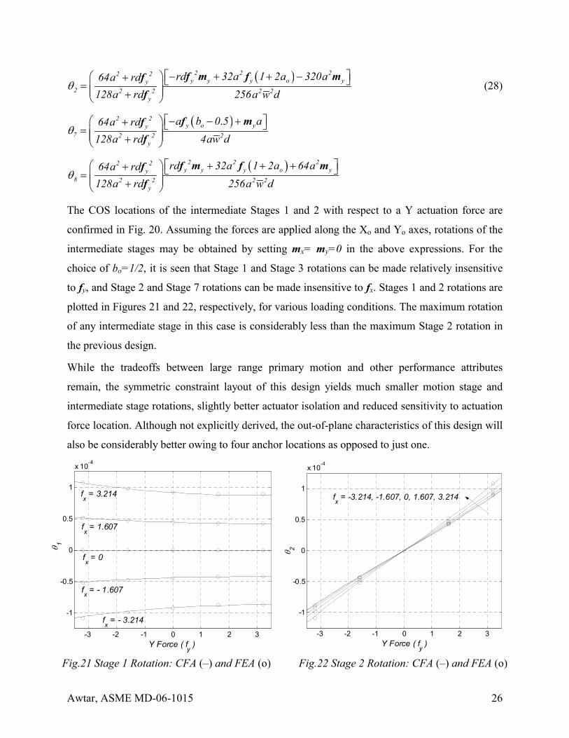
The COS locations of the intermediate Stages 1 and 2 with respect to a Y actuation force are
confirmed in Fig. 20. Assuming the forces are applied along the Xo and Yo axes, rotations of the
intermediate stages may be obtained by setting mx= my=0 in the above expressions. For the
choice of bo=1/2, it is seen that Stage 1 and Stage 3 rotations can be made relatively insensitive
to fy, and Stage 2 and Stage 7 rotations can be made insensitive to fx. Stages 1 and 2 rotations are
plotted in Figures 21 and 22, respectively, for various loading conditions. The maximum rotation
of any intermediate stage in this case is considerably less than the maximum Stage 2 rotation in
the previous design.
While the tradeoffs between large range primary motion and other performance attributes
remain, the symmetric constraint layout of this design yields much smaller motion stage and
intermediate stage rotations, slightly better actuator isolation and reduced sensitivity to actuation
force location. Although not explicitly derived, the out-of-plane characteristics of this design will
also be considerably better owing to four anchor locations as opposed to just one.
-3 -2 -1 0 1 2 3
-1
-0.5
0
0.5
1
x 10-4
Y Force ( fy )
θ 1
fx = 3.214
fx = 1.607
fx = - 1.607
fx = - 3.214
fx = 0
-3 -2 -1 0 1 2 3
-1
-0.5
0
0.5
1
x 10-4
Y Force ( fy )
θ 2
fx = -3.214, -1.607, 0, 1.607, 3.214
Fig.21 Stage 1 Rotation: CFA (–) and FEA (o) Fig.22 Stage 2 Rotation: CFA (–) and FEA (o)

Awtar, ASME MD-06-1015 27
4. FEA and Experimental Results
A thorough Finite Element Analysis has been performed in ANSYS for both designs to validate
the closed-form analysis (CFA) results. BEAM4 elements have been used with the large
displacement option turned on and shear coefficients set to zero. The material assumed in both
cases is AL6061 and the standard values for Young’s Modulus (69,000 N.mm–2) and Poisson’s
Ratio (0.3) are used. The characteristic beam length in both cases is 47.5mm, beam height is
25mm, and the remaining geometric parameters are listed below.
ao 0.9737 ro 0.9737 w1 0.3882 t 1/76
bo 0.5 so 0.9105 w2 0.2697
XY Mechanism Design 1
ao 0.9737 sx 1.3421 w1 0.3882 t 1/76
bo 0.5 sy 1.1316 w2 0.2697 ro 0.9737
XY Mechanism Design 2
The geometric parameters for the two designs are kept identical or as close as possible to provide
an even comparison. The closed-form analysis (CFA) and FEA predictions are found to be in
close agreement. Significantly, the fairly complex and non-intuitive non-linear trends in the
force-displacement relationships have been captured accurately and parametrically by the CFA.
For Design 1, the difference between the predictions of the two analysis methods in terms of the
primary motion, cross-axis error, lost motion, actuator isolation, motion stage rotation, and
intermediate stage rotations is less than 0.5%, 15%, 4%, 2%, 2%, and 0.5%, respectively, over a
primary motion range of ± 0.1. For Design 2, except for the motion stage rotation, which is too
small for a reasonable comparison, the remaining performance predictions using the CFA are
within 0.3%, 4%, 4%, 1%, and 7%, respectively, of the FEA.
To experimentally verify these analytical predictions, an AL6061-T6 prototype of the XY
Mechanism Design 2, with the above-mentioned dimensions, was fabricated using wire-EDM.
The experimental set-up, shown in Fig. 23, has been designed such that the flexure stage can be
actuated using free weights, motorized precision micrometers, and piezoelectric stacks. The
metrology consists of plane-mirror laser interferometry, autocollimation and capacitance gages,

Awtar, ASME MD-06-1015 28
to characterize the translations and rotations of the motion stage and intermediate stages.
Measurements were conducted on an isolation table, and corrected for temperature and humidity
variations. Simultaneous measurements using multiple sensors and successive measurements
using different actuators yield a reliable performance characterization. Measurement uncertainty
is approximately 50nm for displacements and 0.2µrad for rotations.
The experimental measurements and analytical predictions for the XY Mechanism Design 2
displacements and rotations agree very well, as seen in Figures 15 through 18. The experiments
yield an approximately 11% higher primary motion stiffness, indicated in Fig. 15, as compared
to the analysis. Since this stiffness comes primarily from the known transverse elastic stiffness
coefficient of the simple beam, a=12, the observed discrepancy is most likely due to the assumed
value of Young's Modulus. The experimental measurements also reveal a normalized elastic
axial stiffness of the double parallelogram flexure modules that is 40% less than the expected
value, as evident from Fig. 17. This confirms that the axial stiffness of the beams, d, is not
sufficient to capture the axial stiffness of the double parallelogram module if the secondary stage
has a finite compliance [21]. The effect of the secondary stage compliance can be easily
incorporated in the proposed analysis. The non-linear components of the cross-axis error motion
and lost motion are measured to be within 5% of the predicted values.
Fig.23 Experimental Set-up
Flexure Plate
Metrology Plate
Actuators
Sensor Mount

Awtar, ASME MD-06-1015 29
5. Conclusion
There are three main contributions in this paper. Key performance attributes and challenges in
XY mechanism design have been explained, and new parallel kinematic XY flexure mechanism
designs based on systematic and symmetric constraint arrangements are proposed. These
constraint arrangements allow large primary motions and small error motions without running
into over-constraint problems. A 300mm x 300mm XY flexure stage with a motion range of
5mm x 5mm, cross-axis coupling, lost motion and actuator isolation better than 1%, and a
motion stage rotation of less than 1 arc sec, has been tested.
Second, this paper presents a parametric non-linear dimensionless analysis procedure for the
performance prediction of beam-based flexure mechanisms. Based on simple yet accurate
approximations for the beam and double parallelogram flexure force-displacement relations, it
captures all the relevant non-linearities in the motion and force ranges of interest. Consequently,
the relatively complex and non-intuitive non-linear trends in the force-displacement relationships
of the proposed mechanisms have been derived to a high degree of accuracy. The nonlinear
analysis reveals the importance of elastokinematic and load-stiffening effects, which are not
captured by a linear analysis. This exposes the latter’s inadequacy in performance evaluation
over large motion ranges. The parametric nature of the analysis not only provides a better
physical understanding of the mapping between the mechanism’s geometry and performance, but
also an ideal basis for shape and size optimization. The presented analysis is general in nature
and remains valid for any beam shape variations.
Finally, we highlight the fact that there exist fundamental performance tradeoffs in flexure
mechanism design, arising from the imperfect constraint properties of flexure elements. The
closed-form force-displacement relationship predictions accurately quantify these performance
attributes and tradeoffs. It is shown that the need to minimize cross-axis coupling, parasitic stage
rotations, lost motion, and loss in actuator isolation and drive stiffness, conflicts with the desire
for a large range of primary motion. These compromises depend on the characteristics of the
individual building-block modules as well as the geometry of the layout. It is shown that Design
2, owing to its higher degree of symmetry, exhibits improved actuator isolation, lower stage
rotations, and a higher degree of robustness against manufacturing and assembly errors, in
comparison to Design 1. However, other performance attributes such as lost motion and drive

Awtar, ASME MD-06-1015 30
stiffness, being strongly dependent on the building-block characteristics, remain similar in nature
and magnitude. It is also shown that the concept of Center of Stiffness may be used as a
convenient means for the passive minimization of stage rotations. However, the effectiveness of
this method is influenced by the mechanism's geometry, with the symmetric design proving to be
a more suitable candidate.
Several avenues for future work are currently being pursued. The compliance of the secondary
stage in the double parallelogram flexure modules can easily by modeled and included in the
closed-form analysis to obtain more accurate and realistic performance predictions. Since certain
performance attributes may not be improved simply by a symmetric geometry of constraint
arrangement, other building blocks may be considered depending upon the requirements of a
given application. For motion stages designed for high dynamic performance, the
elastokinematic drive stiffness can be considerably improved by the use of the double tilted-
beam flexure module [12], which preserves axial stiffness but is detrimental to parasitic stage
rotations. Furthermore, beam shape optimization allows for the fine-tuning of the beam
characteristic coefficients to achieve specific improvements in the performance attributes.
To facilitate the nonlinear analysis, we are developing a symbolic computation tool in MAPLETM
that would allow a quick performance evaluation of any 2-D beam-based flexure design concept.
It may be noticed that the system equations have been explicitly solved to arrive at the force-
displacement results. The use of energy methods can prove to be tricky in problems with
elastokinematic non-linearities and is currently being explored in order to make the analysis
more efficient. The elastokinematic and load-stiffening effects lead to stiffness variations and
couplings between displacement coordinates, thereby significantly affecting the dynamic
characteristics of the proposed designs. An accurate dynamic model of the mechanisms that
incorporates these effects is necessary for the design of a high-precision high-bandwidth motion
system, and is being developed. For high-precision applications, the determination of thermal
sensitivity is also a key requirement and may be incorporated within the proposed analysis
framework.

Awtar, ASME MD-06-1015 31
References
1. Ryu, J.W., Gweon, D.-G., and Moon, K.S., 1997, “Optimal Design of a Flexure Hinge
based X-Y-θ Wafer Stage”, Journal of Precision Engineering, 21(1), pp. 18-28.
2. Smith, A.R., Gwo, S., and Shih, C.K. 1994, “A New High Resolution Two-dimensional
Micropositioning Device for Scanning Probe Microscopy”, Review of Scientific
Instruments, 64 (10), pp. 3216-3219.
3. Eom, T.B. and Kim, J.Y., 2001, “Long Range Stage for the Metrological Atomic Force
Microscope”, Proc. ASPE 2001 Annual Meeting, pp. 156-159.
4. Gorman, J. J. and Dagalakis, N. G., 2003, “Force control of linear motor stages for
microassembly”, IMECE2003-42079, ASME International Mechanical Engineering
Conference and Exposition, Washington, DC.
5. Vettiger, P., et al., 2000, “The Millipede – More than one thousand tips for future AFM data
storage”, IBM Journal of Research and Development, 44 (3), pp. 323-340.
6. ADXL Accelerometers and ADXRS Gyroscopes, www.analogdevices.com
7. Agilent Nanostepper J7220, www.labs.agilent.com
8. XY Nanopositioner P-733, www.physikinstrumente.com
9. Chang, S.H., Tseng, C.K., and Chien, H.C., 1999, “An Ultra-Precision XYθZ Piezo-
Micropositioner Part I: Design and Analysis”, IEEE Transactions on Ultrasonics,
Ferroelectrics, and Frequency Control, 46 (4), pp. 897-905.
10. Chen, K.S., Trumper, D.L., and Smith, S.T., 2002, “Design and Control for an
Electromagnetically driven X-Y-θ Stage”, Journal of Precision Engineering and
Nanotechnology, 26, pp. 355-369.
11. Awtar, S., 2004, “Analysis and Synthesis of Planer Kinematic XY Mechanisms”, Sc.D.
thesis, Massachusetts Institute of Technology, Cambridge, MA.
(http://web.mit.edu/shorya/www)
12. Awtar, S. and Slocum, A.H., 2005, “Closed-form Nonlinear Analysis of Beam-based
Flexure Modules”, Proc. ASME IDETC/CIE 2005, Long Beach, CA, Paper No. 85440

Awtar, ASME MD-06-1015 32
13. Ananthasuresh, G.K., Kota S., and Gianchandani, Y., 1994, “A Methodical Approach to
Design of Compliant Micromechanisms”, Solid State Sensor and Actuator Workshop, Hilton
Head Island, SC, pp. 189-192.
14. Frecker, M.I., Ananthasuresh, G.K., Nishiwaki, S., Kickuchi, N., and Kota S., 1997,
“Topological Synthesis of Compliant Mechanisms Using Multi-criteria optimization,”
Journal of Mechanical Design, 119, pp. 238-245.
15. Blanding, D.K., 1999, Exact Constraint: Machine Design Using Kinematic Principles,
ASME Press, New York, NY.
16. Awtar S., and Slocum A.H., 2004, “Apparatus Having motion with Pre-determined degree
of Freedom”, US Patent 6,688,183 B2.
17. Bisshopp, K.E., and Drucker, D.C., 1945, “Large Deflection of Cantilever Beams”,
Quarterly of Applied Mathematics, 3 (3), pp. 272-275.
18. Howell L.L, 2001, Compliant Mechanisms, John Wiley & Sons, New York, NY.
19. Plainevaux, J.E., 1956, “Etude des deformations d’une lame de suspension elastique”,
Nuovo Cimento, 4, pp. 922-928.
20. Legtenberg, R., Groeneveld, A.W. and Elwenspoek, M., 1996, “Comb-drive Actuators for
Large Displacements”, Journal of Micromechanics and Microengineering, 6, pp. 320-329.
21. Saggere, L., Kota, S., 1994, “A New Design for Suspension of Linear Microactuators”,
ASME Journal of Dynamic Systems and Control, 55 (2), pp. 671-675.
Awtar, ASME MD-06-1015 33
List of Figure Captions
Fig.1 Proposed Constraint Arrangement for XY Flexure Mechanisms
Fig.2 XY Flexure Mechanism Design 1
Fig.3 XY Flexure Mechanism Design 2
Fig.4 Double Parallelogram Flexure Module
Fig.5 XY Mechanism 1 in a Deformed Configuration
Fig.6 Primary Motion: CFA (–) and FEA (o)
Fig.7 Cross-Axis Error Motion: CFA (–) and FEA (o)
Fig.8 Lost Motion / Drive Stiffness: CFA (–) and FEA (o)
Fig.9 Actuator Isolation: CFA (–) and FEA (o)
Fig.10 Motion Stage Rotation: CFA (Contour), CFA (–) and FEA (o)
Fig.11 Moment Sensitivity and COS for the Stages with respect X Force: CFA (–) and FEA (o)
Fig.12 Stage 1 Rotation: CFA (–) and FEA (o)
Fig.13 Stage 2 Rotation: CFA (–) and FEA (o)
Fig.14 XY Mechanism 2 in a Deformed Configuration
Fig.15 Primary Motion: CFA (–), FEA (o), Exp (*)
Fig.16 Cross-axis Error Motion: CFA (–), FEA (o), Exp (*)
Fig.17 Lost Motion / Drive Stiffness: CFA (–), FEA (o), Exp (*)
Fig. 18 Actuator Isolation: CFA (–), FEA (o), Exp (*)
Fig.19 Motion Stage Rotation: CFA (Contour), CFA (Lines) and FEA (Marks)
Fig.20 Moment Sensitivity and COS for the Stages with respect Y Force: CFA (–) and FEA (o)
Fig.21 Stage 1 Rotation: CFA (–) and FEA (o)
Fig.22 Stage 2 Rotation: CFA (–) and FEA (o)
Fig.23 Experimental Set-up