A&A 599, A17 (2017)DOI: 10.1051/0004-6361/201629464c© ESO 2017

Astronomy&Astrophysics

Constraining the thin disc initial mass function using Galacticclassical Cepheids

R. Mor1, A. C. Robin2, F. Figueras1, and B. Lemasle3

1 Dept. Física Quàntica i Astrofísica, Institut de Ciències del Cosmos, Universitat de Barcelona (IEEC-UB), Martí Franquès 1,08028 Barcelona, Spaine-mail: rmor@fqa.ub.edu

2 Institut Utinam, CNRS UMR6213, Université de Bourgogne Franche-Comté, OSU THETA, Observatoire de Besançon,BP 1615, 25010 Besançon Cedex, France

3 Astronomisches Rechen-Institut, Zentrum für Astronomie der Universität Heidelberg, Mönchhofstr. 12–14, 69120 Heidelberg,Germany

Received 3 August 2016 / Accepted 20 October 2016

ABSTRACT

Context. The initial mass function (IMF) plays a crucial role in galaxy evolution and its implications on star formation theory makeit a milestone for the next decade. It is in the intermediate and high mass ranges where the uncertainties of the IMF are larger. This isa major subject of debate and analysis both for Galactic and extragalactic science.Aims. Our goal is to constrain the IMF of the Galactic thin disc population using both Galactic classical Cepheids and Tycho-2 data.Methods. For the first time, the Besançon Galaxy Model (BGM) has been used to characterize the Galactic population of classicalCepheids. We modified the age configuration in the youngest populations of the BGM thin disc model to avoid artificial discontinuitiesin the age distribution of the simulated Cepheids. Three statistical methods, optimized for different mass ranges, have been developedand applied to search for the best IMF that fits the observations. This strategy enables us to quantify variations in the star formationhistory (SFH), the stellar density at Sun position and the thin disc radial scale length. A rigorous treatment of unresolved multiplestellar systems has been undertaken, adopting a spatial resolution according to the catalogues used.Results. For intermediate masses, our study favours a composite field-star IMF slope of α = 3.2 for the local thin disc, excludingflatter values, e.g. the Salpeter IMF (α = 2.35). Our findings are broadly consistent with previous results derived from Milky Waymodels. Moreover, a constant SFH is definitively excluded, the three statistical methods considered here show that it is inconsistentwith the observational data.Conclusions. Using field stars and Galactic classical Cepheids, we found an IMF steeper than the canonical stellar IMF of associationsand young clusters above 1 M�. This result is consistent with the predictions of the integrated Galactic IMF.

Key words. stars: luminosity function, mass function – stars: variables: Cepheids – Galaxy: disk – solar neighborhood –Galaxy: evolution

1. Introduction

Classical Cepheids are probably the best-known and most impor-tant pulsating variable stars. Since Henrietta Swan Leavitt deter-mined for the first time, in 1912, their period-luminosity relation(Leavitt & Pickering 1912), classical Cepheids have become thefirst ladder of the extragalactic distance scale, since they provideaccurate distances in the Local Universe. Now, in the Gaia era,the expected thousands of Cepheids that are going to be detected(Eyer & Cuypers 2000; Windmark et al. 2011; Mor et al. 2015),again place these classical variable stars in a privileged positionwhen studying the structure of the Milky Way. In this work weplan to update the youngest populations in the Besançon GalaxyModel (BGM) making it capable to simulate a reliable popula-tion of Cepheids. With this new configuration, and as a first step,we aim to use the classical Cepheids as tracers of intermediate-mass population to constrain the initial mass function (IMF) ofthe thin disc.

The IMF describes the mass distribution of a star formationepisode. Together with the star formation history (SFH), it is oneof the most important functions to characterize the evolution ofthe stellar populations in the Milky Way and external galaxies.

The chemical composition and luminosity of galaxies is directlyinfluenced by the IMF as it determines the baryonic content andthe light of the Universe. Salpeter (1955) was the first to describethe IMF as a simple power law dN = ξ(m)dm = km−αdm and heestimated a power-law index of α = 2.35, taking into considera-tion an age of 6 Gyr for the Milky Way. Since then, several fun-damental works on the empirical derivation of the Galactic IMFhave been written, such those of Schmidt (1959), Miller & Scalo(1979), Scalo (1986), Kroupa et al. (1993), and Kroupa (2002)among others. Even so, the shape of the IMF is still a matter ofdebate, in particular for the high and intermediate stellar massrange.

Several methods to derive the IMF consist either in analysingthe mass distribution of complex preprocessed samples, or byfitting models to star counts in complete but limited samples.Advantages and drawbacks of this last method are discussed inthis paper, keeping in mind that this approach depends on otherparameters such as the SFH, the density distribution, or the in-terstellar extinction.

An important handicap when studying the IMF at intermedi-ate and high masses is the low number of stars of these massesthat can be found in clusters or associations. The same occurs

Article published by EDP Sciences A17, page 1 of 12

A&A 599, A17 (2017)

when using field stars just around few hundred parsecs from theSun. Classical Cepheids can solve the problem of poor statisticsat intermediate masses because they are bright and their distancecan be accurately determined. Soon Gaia will provide us withthousands of them, but for the moment the most complete cata-logues of Galactic classical Cepheids provide us with hundredsof Cepheids in the intermediate stellar mass range. These hun-dreds of Cepheids, together with the ≈800 000 stars from theTycho-2 catalogue (Høg et al. 2000) up to V = 11 (that is domi-nated by low-mass stars), ensures good statistics to constrain theIMF in the present work.

It have been suggested that the IMF is closely related tothe structure and fragmentation mechanism of molecular cloudswhere the stars are formed. Thus, several attempts to derive theIMF theoretically have been made in this context. For example,Adams & Fatuzzo (1996) computed a semi-empirical mass for-mula (SEMF) which provides the transformation between initialconditions in molecular clouds and the final masses of formingstars based on the idea that stars determine their own massesthrough the action of powerful stellar outflows. For a particu-lar SEMF, a given distribution of initial conditions theoreticallypredicts a corresponding IMF. Key works when discussing thetheory of the IMF are the following: Larson (1992), assuminga two-dimensional molecular cloud and hierarchical fragmenta-tion, derived a slope of α = 3 for high masses and α = 3.3 for amore general IMF. In contrast, Padoan & Nordlund (2002), con-sidering a turbulent fragmentation of molecular clouds, derivedan IMF with a slope α = 2.33, significantly lower and very closeto the Salpeter one. Elmegreen (1997) obtained a slope valueof α ≈ 2–2.7 considering a turbulent fractal molecular cloud.We need to bear in mind that several parameters are degener-ated when deriving the theoretical formation of the stellar coresfrom the molecular clouds, i.e. coalescence of protostellar cores,mass-dependence, accretion process, stellar feedback, or frag-mentation. In the case of intermediate and high-mass stars theformation process is even more complex. Thus, in this context,the empirical and semi-empirical determination of the IMF at in-termediate and high masses can contribute to the understandingof the star formation mechanism.

From a population synthesis point of view, several attemptshave made to determine the IMF for different components ofthe Milky Way. For example in Reylé & Robin (2001) andRobin et al. (2014), the IMF of the thick disc component wasstudied using deep star counts in different directions. Moreoverin Robin et al. (2000), the halo IMF was investigated. Recentlythe IMF of the thin disc was evaluated by our team (Czekaj et al.2014) using Tycho-2 data and also by Rybizki & Just (2015) us-ing an observational sample that consists of stars from the ex-tended Hipparcos catalogue and the Catalogue of Nearby Stars.

In this work, we aim to constrain the thin disc IMF at inter-mediate masses using the BGM. This tool is being updated eachyear by studying the different components of the Milky Way,e.g. the bulge region (Robin et al. 2012b), where a triaxial boxyshape for the bar is fitted; the thick disc, Robin et al. (2014),where two successive star formation episodes are proposed; thethin disc (Czekaj et al. 2014), where results point to a decreasingSFH whatever IMF is assumed. Furthermore the BGM has beenused to study the interstellar medium (Marshall et al. 2006),Galactic kinematics and dynamics (e.g. Bienaymé et al. 2015),to estimate micro-lensing probabilities (Awiphan et al. 2016;Kerins et al. 2009) and it has has also been used for the prepara-tion of the ESA Gaia astrometric mission (Robin et al. 2012a).In a daily effort to update the BGM piece by piece, contributingstep by step to the knowledge of the different components of the

Milky Way, in this work we aim to update the youngest popu-lations of the BGM thin disc, improving its fit with the Tycho-2data and using it to constrain the IMF.

In Sect. 2, we briefly describe the BGM, the model ingredi-ents, the characteristics of classical Cepheids in the BGM andour strategy. In Sect. 3, we describe the observational sample.In Sect. 4, we present our evaluation methods. Results are pre-sented in Sect. 5, while discussion and conclusions are presentedin Sects. 6 and 7.

2. The Besançon Galaxy Model

The Besançon Galaxy Model has proved to be an efficient toolto test the Milky Way galaxy structure and evolution scenarios.Last updates are described in Robin et al. (2003), Robin et al.(2012b), Robin et al. (2014) and Czekaj et al. (2014), whereasits dynamical consistency is discussed in Bienaymé et al. (1987)and Bienaymé et al. (2015). In this study, we are interested ingenerating a full sky set of data to be compared with bothTycho-2 data and the most complete catalogues of GalacticCepheids. These catalogues are complete up to a bright limit inapparent magnitude, thus with a dominant contribution from thethin disc population and a small contribution from the thick disc(expected ≈10%) and the halo (expected ≈0.3%).

2.1. The thin disc population

The thin disc component is described in Czekaj et al. (2014). Thestars are generated following an IMF and an SFH, with a con-tinuous star formation during the disc evolution. The thin discpopulation is divided into seven age sub-populations with theage intervals described in Bienaymé et al. (1987). The densitydistribution of each sub-population of the thin disc is assumedto follow an Einasto density profile as described in Robin et al.(2012b) Sect. 2.1, except for the youngest sub-population whichfollows the expression described in Robin et al. (2003). Themain parameters for the characterization of the Einasto profilesare the eccentricities of the ellipsoid (ε, that is the axis ratio), thescale length of the disc (Rd) and the scale length of the disc hole(Rh). A velocity dispersion as a function of age is adopted and,each time the IMF and the SFH is changed, new structure pa-rameters (e.g. the eccentricities of the ellipsoids ε) are computedto keep the dynamical statistical equilibrium (Bienaymé et al.1987). Stellar evolutionary tracks and model atmosphere, com-bined with an age-metallicity relation, enable us to go frommasses, ages, and metallicities to the space of the observables.In this process a 3D interstellar extinction model is assumed.

BGM thin disc simulations work following the scheme ofFig. 3 from Czekaj et al. (2014). The SFH, a key ingredient ofthe simulation, determines the amount of stars generated in eachone of the seven age sub-populations. Once a star is created, weassign an age and a metallicity to it. The ages are drawn ran-domly from the uniform distribution in the interval of the givenage sub-population. The metallicity is drawn for each star fromits own age, according to the age-metallicity relation adopted.When the age, mass, and metallicity are established, we inter-polate the stellar evolutionary tracks and find the position of thestar in the Hertzsprung-Russell diagram.

The model includes the generation of unresolved and re-solved binary systems according to an imposed spatial resolu-tion. The binarity treatment is well described in Sects. 2.2.2 and4.3. of Czekaj et al. (2014). Binaries are generated following thescheme proposed by Arenou (2011), also used to generate the

A17, page 2 of 12

R. Mor et al.: Constraining the IMF using Galactic Cepheids

Gaia Universe Model (Robin et al. 2012a). To decide if eachnewly created star is either a single or primary component ofmultiple system, the model uses a probability density functionthat depends on the mass of the object and its luminosity class.The mass-ratio distribution between system components, esti-mated from observations (Arenou 2011), takes into account thespectral type and mass of the primary component.

Hereafter, our initial default model (hereafter DM) will beModel B of Czekaj et al. (2014). Model B is the model proposedin Czekaj et al. (2014), which gave better results in differentstudies (e.g. Robin et al. 2014), moreover it is used nowadays asthe thin disc model for the Gaia Object Generator (Robin et al.2012b; Luri et al. 2014). Table 5 of Czekaj et al. (2014) showsthe set of thin disc ingredients adopted to fit Tycho-2 data us-ing the radial scale length parameters detailed in Robin et al.(2003). The stellar evolutionary models used are those ofChabrier & Baraffe (1997) for M < 0.7 M�, Bertelli et al. (2008,2009) for 0.7 M� < M < 20 M�, and Bertelli et al. (1994)20 M� < 120 M�.

2.2. Generation of classical Cepheids

The instability strip (IS) is the region of the Hertzprung-Russeldiagram occupied by the pulsating variable stars, including clas-sical Cepheids. The hotter and cooler boundaries of the IS arecalled the blue edge and red edge, respectively. For this work, upto apparent magnitude V = 9, that is for stars around solar neigh-bourhood, we adopt the blue edge as log(Teff) = −(log(L/L�) −62.7)/15.8 from Bono et al. (2000b) and red edge as log(Teff) =−(log(L/L�) − 40.2)/10.0 from Fiorentino et al. (2013), bothderived from Cepheid pulsation models at solar metallicity. ForCepheids at larger heliocentric distances (magnitudes 9 < V ≤12), and given the radial metallicity gradient of the Milky Way(e.g. Genovali et al. 2014), we decided to keep the same red ageand to use as the blue edge the one derived from pulsation mod-els at lower metallicity (z = 0.008) from Fiorentino et al. (2013),that is log(Teff) = −(log(L/L�) − 52.5)/13.1.

We impose a luminosity cut in the range 2.7 ≤ log(L/L�) ≤4.7. This luminosity cut constrains the effective temperature ofthe Cepheids to about 4000 ≤ Teff ≤ 7000 K (Bono et al. 1999).

The masses of our simulated Cepheids, selected with theboundaries of the IS described above, are found to be between3 and 11 M� with a few reaching up to 15 M� (see Fig. 1).These values are in good agreement with the mass ranges in theliterature. To start with, the classical review from Cox (1980)established the Cepheid mass range between 3 and 15 M�.More recent studies, such as Caputo et al. (2005), found massesbetween 5 to 15 M�. Using evolutionary models, Bono et al.(2000a) estimated a minimum mass of ≈3.25 M� for low metal-licity Cepheids and ≈4.75 M� for Cepheids with solar metal-licity. The upper limit given by both Bono et al. (2000a) andAlibert et al. (1999) could depend on metallicity and it is in therange 10−12 M�. More recently, Anderson et al. (2014), also us-ing stellar model but including stellar rotation, predict massesfrom 4 to 10 M�. This agreement between literature and ourgenerated Cepheid mass distribution using the BGM reinforceboth the boundaries of the IS adopted and the BGM Cepheid-generation strategy.

The age distribution of our simulated Cepheids is presentedin Fig. 2. Most of our simulated Cepheids have ages of be-tween 20 and 200 Myr, well compatible with the values de-rived by Bono et al. (2005), who estimated ages from ≈25 Myrto ≈200 Myr, based on evolutionary and pulsation models. The

Fig. 1. Mass distribution of the simulated Galactic classical Cepheidsfor 10 runs. The plot corresponds to the default model. The mass isexpressed in solar masses.

shape of the age distribution obtained here using BGM is dis-cussed in Sect. 2.3.

With regard to binary fraction, our simulations show thatabout 68% of classical Cepheids are contained in a binary sys-tem. This percentage is consistent with values from the litera-ture (e.g. Szabados 2003 estimated about 60–80% of Cepheids).None of our simulated Cepheids are secondary components ofa multiple system. To generate these objects as secondaries, pri-mary stars should have M > 3.5 M� and we have checked thatonly about 2% of stars up to V = 12 fulfil this condition. Further-more, this probability becomes negligible when imposing thesecondary to be in the instability strip.

Czekaj et al. (2014) adopted a spatial resolution of 0.8 arcsecaccording to the resolution of Tycho-2 catalogue. In the citedwork, it was noted that most of the simulated binaries have an-gular separation smaller than 0.5 arcsec. The Cepheid cataloguesused here could have worse resolutions than Tycho-2, thus thedistribution of the simulated angular separation enables us toadopt the same 0.8 arcsec resolution for the Cepheids withoutcompromising the total number of star counts.

2.3. Cepheid ages to constrain the BGM youngestpopulations

In Fig. 2, we show the age distribution of the simulated classi-cal Cepheids with a black dotted line up to apparent magnitudeV = 12 using the DM. Like the other stars, the Cepheids are gen-erated following an SFH and an IMF, as described in Sect. 2.1.Since classical Cepheids are young stars they belong to the sub-population 1 and 2 of the thin disc component of the BGM. Al-though the range of the ages shown in Fig. 2 is compatible withthe ages of Cepheids (Bono et al. 2005), its distribution presentsa double peak which has not been seen in the empirical data.This is an artefact that comes from a discontinuity between sub-populations 1 and 2 of the thin disc in the BGM. In the presentwork, we modified the age interval of these two youngest sub-populations to avoid this discontinuity. In the initial DM, thefirst population covered an age interval between 0 and 0.15 Gyr,while the second sub-population covered the age range 0.15 to1 Gyr. From now on, the age range of the first sub-population

A17, page 3 of 12

A&A 599, A17 (2017)

Fig. 2. Age distribution of the simulated Galactic classical Cepheids for10 runs. The black dotted line is for the initial default model. The redsolid line is for the modified default model after the update of the ageintervals of the youngest populations of the BGM.

and second sub-population of our DM will be set from 0.0 to0.10 Gyr and between 0.10 to 1 Gyr respectively. Thus, once theage interval for sub-population 1 and 2 is redefined, all the ma-chinery of the BGM is set up and rerun, e.g. the amount of starsgenerated in the so-called new sub-population 1 and 2 is derivedfrom the SFH, and the integrals over time will be computed ac-cording to the new age range. A new BGM simulation is usedto update the Cepheid age distribution. In Fig. 2, we show in redthe age distribution of the simulated Galactic classical Cepheidswith the revised DM. Now the age distribution follows a smoothsingle peak distribution. As seen in Sect. 5, this modification ofthe age ranges improves the fit of the BGM with Tycho-2 data inthe Galactic plane.

2.4. Model variants and strategy

In Fig. 3, we present the scheme of the seven model variantsproposed to constrain the thin disc IMF. To evaluate which is thebest of the tested IMFs (see Sect. 2.5) it is mandatory to analysenot only the changes that are due to the IMF, but also evaluatethe impact of other key ingredients on the mean properties of thesimulated catalogues. Work performed in Czekaj et al. (2014),Robin et al. (2012b), and previous experience has allowed us toidentify the SFH, the stellar density at the Sun position, and theradial scale length as the key parameters most affecting the starcount analysis that we perform in this paper.

By departing from the DM, changing only the IMF, we con-structed the two other main model variants (see Fig. 3). Thoseare the Salpeter Variant (SV) and the Haywood-Robin variant(HRV). In Sect. 2.5, we further describe the IMFs used. Theimpact of thin disc radial scale length variations is tested, as-suming the scale length of Robin et al. (2003; Rd = 2530 pcand Rh = 1320 pc) for the DM and changing it to the values ofRobin et al. (2012b; Rd = 2170 pc and Rh = 1330 pc) in thedefault model A variant (DAV). These new scale lengths havebeen obtained by fitting 2MASS data towards the bulge regionin Robin et al. (2012b). To evaluate the effects of the variationin the local stellar mass density, we tested the values of Wielen(1974; 0.039 M�/pc3 ) in the default model B variant (DBV) andJahreiß & Wielen (1997; 0.033 M�/pc3) used in the DM. Both

values are selected because they are used in the best-fit mod-els in Czekaj et al. (2014) and they represent a good range ofthe values published in the literature. To analyse the effects pro-duced by changes in the SFH, we assumed the decreasing SFHby Aumer & Binney (2009) for the DM and a constant SFH inthe default model C variant (DCV). Additionally, to further studythe Haywood-Robin IMF, we test the variant HRVB, which hasthe HRV parameters but using 0.039 M�/pc3 as the local stellarmass density.

For the sky areas with longitude between –100 and 100and latitudes between –10 and 10 the model variants presentedin Fig. 3 have been tested with two different extinction mod-els, Marshall et al. (2006) and Drimmel & Spergel (2001). Us-ing this strategy, we are able to identify what the impact of theinterstellar extinction is in our Cepheids data, most of them con-tained in the Galactic plane. All the other thin disc model in-gredients are maintained as fixed. Its values are those adoptedby Czekaj et al. (2014), Tables 2 and 5. Once a full set of pa-rameters is adopted, thus for each of the seven variant mod-els in Fig. 3, we applied dynamical constraints as described inBienaymé et al. (1987), solving the Poisson equation, using theCaldwell & Ostriker (1981) rotation curve for constraining thedark halo density, and deriving the eccentricities of the Einastoprofiles for each thin disc sub-component from the collision-less Boltzmann equation, assuming dynamical statistical equi-librium. The resulting values for the Einasto eccentricities aregiven in Tables 1 and 2.

2.5. Initial mass function

In Fig. 4, we present the normalised IMFs that we proposed totest. They are described using the classical analytical approxi-mation ξ(m):

dNdm

= ξ(m) = k · m−α = k · m−(1+x) (1)

where N is the number of stars, m is the mass (in M�), and k isthe normalisation constant. We propose to check the two IMFsthat better fit the Tycho-2 data (Czekaj et al. 2014). The slope ofthese IMFs at intermediate masses are on the upper limit valuesfound in the literature (see Kroupa 2002). Additionally, to covermost of the range of variation of the slope, we include the clas-sical IMF of Salpeter (1955) with α = 2.35, as representative ofthe lowest values. In Table 3, we present the slopes and limitingmasses for the tested IMFs.

In Fig. 4, we present the three tested IMFs normalized inthe range between 0.09 and 120 M�. The normalization hasbeen done in terms of mass. To get the mass locked withineach mass interval, one must solve

∫m · ξ(m)dm for each mass

range. The sum of the obtained result for each mass interval isthen normalized to one using the continuity coefficients Ki as∑

i Ki ·∫ mi+1

mim · ξ(m)dm = 1, i being the index of the mass in-

terval considered (i = 1, 3), see Czekaj et al. (2014) Sect. 2.2.1.Looking at Fig. 4, we can anticipate the general lines of the sim-ulations. Salpeter IMF will produce more stars in the range be-tween 0.09 and 0.5 M� while in the range between 0.5 to about5 M�, it will produce less stars than the two other tested IMFs.From about 5 M� to 120 M�, Salpeter IMF will be the IMF thatproduces more stars. If we take a look at the tested IMFs inthe Cepheid mass range, it is clear that Salpeter will dedicatemore mass to the Cepheid production than the other two IMFs.We note, however, that the Salpeter IMF generates less low-mass Cepheids (in the range ≈3 M� to ≈6 M�) and much more

A17, page 4 of 12

R. Mor et al.: Constraining the IMF using Galactic Cepheids

Fig. 3. Scheme of the seven model variants tested in the present paper. For the three main variants, DM, HRV, and SV only the IMF has beenchanged. The DCV differs from the DM in the SFH, DBV differs from DM in the stellar density at Sun position, and DAV differs from DM on thethin disc radial scale length. The HRV has its own variant in stellar density at Sun position, the HRVB.

Table 1. Thin disc local densities M�/pc3.

Sub-population Age (Gyr) DM HRV DBV DCV HRVB SV DAV1 0–0.10 0.00131 0.00117 0.00147 0.00207 0.00133 0.00113 0.001282 0.10 –1 0.00541 0.00504 0.00639 0.00808 0.00589 0.00468 0.005303 1–2 0.00427 0.00404 0.00499 0.00557 0.00483 0.00382 0.004174 2–3 0.00291 0.00284 0.00351 0.00339 0.00341 0.00275 0.002925 3–5 0.00496 0.00502 0.00580 0.00485 0.00596 0.00496 0.004986 5–7 0.00510 0.00526 0.00601 0.00393 0.00620 0.00535 0.005067 7–10 0.00944 0.00997 0.01122 0.00543 0.01183 0.0103 0.00953

Total thin disc 0.0334 0.0333 0.0394 0.0333 0.0395 0.0330 0.0332

Notes. Contribution to the total dynamical mass of the 7 sub-populations (see Sect. 2.1) for each one of the model variants in Fig. 3.

Table 2. Thin disc eccentricities of the 7 sub-populations (see Sect. 2.1) for each one of the model variants in Fig. 3.

Sub-population Age (Gyr) DM HRV DBV DCV HRVB SV DAV1 0–0.10 0.0140 0.0140 0.0140 0.0140 0.0140 0.0140 0.01402 0.10–1 0.0205 0.0204 0.0197 0.0210 0.0196 0.0205 0.02313 1–2 0.0292 0.0292 0.0281 0.0299 0.0280 0.0292 0.03274 2–3 0.0441 0.0440 0.0426 0.0450 0.0424 0.0441 0.04895 3–5 0.0565 0.0564 0.0547 0.0576 0.0545 0.0565 0.06246 5–7 0.0642 0.0641 0.0622 0.0654 0.0619 0.0642 0.07077 7–10 0.0647 0.0645 0.0627 0.0659 0.0624 0.0646 0.0712

high-mass Cepheids (M > 6 M�) than the other tested IMFs.Kroupa-Haywood IMF will produce a few more Cepheids thanHaywood-Robin IMF.

3. Classical Cepheid observational dataOur strategy requires us to compare well-defined samples whichare complete up to a limit in apparent magnitude. Whereas thisis trivial for simulated BGM samples, observational data haveto be treated rigorously. Currently, the most complete Cepheidcatalogues with good Cepheid variability classification are theBerdnikov catalogue (Berdnikov 2008) with 577 stars and theDDO catalogue (Fernie et al. 1995) with 509 stars, with bothcatalogues being compilations of photometric data for knownCepheids. We tested that 95% of Cepheids up to V = 9are contained in both catalogues, thus in the present work we

have used the photometric data from the Berdnikov catalogue(for Cepheids up to V = 9) since it is the most up-to-dateone. For fainter magnitudes, we used the ASAS Catalogue ofVariable Stars (hereafter ACVS) from Pojmanski (2002) andPojmanski et al. (2006). The telescopes for this survey are in-stalled in the southern hemisphere from where stars with decli-nation δ ≤ 29 can be observed. ACVS contains 809 stars classi-fied exclusively as classical Cepheids. Whereas the quality of thelight curves in the Bernikov catalogue ensures the stars are wellclassified as classical Galactic Cepheids, the classification in theACVS catalogue, which is built using small telescopes thus hav-ing less accurate light curves, could contain some contaminantsfrom other variable types. To minimize the contamination, wework only with those Cepheids in ACVS that are concentratedin the Galactic plane.

A17, page 5 of 12

A&A 599, A17 (2017)

Table 3. Slopes and mass limits for the tested IMFs.

IMF M1 α1 M2 α2 M3 α3 M4

Salpeter 0.09 2.35 – 2.35 – 2.35 120Haywood-Robin 0.09 1.6 1.0 3.0 – 3.0 120

Kroupa-Haywood 0.09 1.3 0.5 1.8 1.53 3.2 120

Notes. The M1, M2, M3, and M4 are the limiting masses (when necessary) and the α1, α2 and α3 are the corresponding slopes. The values of theM1 and M4 are fixed according to the limiting masses of the evolutionary tracks.

-5

-4

-3

-2

-1

0

1

0.1 1 1.53 3 4 6 8 14 50 100

log

(m−

x )

Mass (M�)

Salpeter IMFKroupa-Haywood IMF

Haywood-Robin IMF

Fig. 4. Three tested IMFs in the range between 0.09 and 120 M� nor-malized. The blue solid line is for Salpeter IMF, the red thick dashed lineis for Kroupa-Haywood, and the green thin dashed line is for Haywood-Robin. We note how for a fix total amount of mass, Salpeter IMF is theIMF that generates less stars in the interval ≈0.5 to ≈6 M�, but morestars at M > 6 M� and at M < 0.5 M�

The type II Cepheids, the old, low-mass counterpart to theclassical Cepheids are believed to belong to the thick disc.They are difficult to disentangle from classical Cepheids. Forthe brightest Cepheids, for which large amounts of photomet-ric data is available and the chemical composition is known (e.g.Andrievsky et al. 2002; Lemasle et al. 2007), the amount of con-tamination from type II Cepheids is negligible. For the faintestCepheids of our sample, since we concentrate on the Galacticplane, where the contribution of the thick disc is small, the con-tamination from type II Cepheids is not significant for our study.

Classical Cepheids are variable stars with large amplitudevariations in visual magnitude. As a result, caution is necessarywhen defining the photometric parameters setting the limitingmagnitude. The Berdnikov catalogue provides both the visualmagnitude at maximum (Vmax) and minimum brightness (Vmin).ACVS provides the visual magnitude at maximum brightness(Vmax) and the amplitude (δV). To accurately determine the meanmagnitude of a Cepheid, template lightcurves should be used.But, as we are conservative when selecting the limiting magni-tude for the completeness of the catalogues, we can approximateVmean by (Vmax + Vmin)/2 for Berdnikov data and by Vmax + δV/2for ACVS. With this definition in mind, several considerationsarise when comparing simulated and observed data.

Since our BGM simulations do not include brightness vari-ability information (see Sects. 2.1 and 2.2), it is appropriate toconsider the magnitude from the evolutionary tracks as the oneassociated to the mean intrinsic brightness of the star. The lightcurve of the Cepheids can be assumed as being symmetric at first

approximation; then the probability of finding a Cepheid in anypoint of its period between Vmax and Vmin is uniform.

Owing to Cepheid variability, one might wonder whethera bias in the star counts similar to Malmquist bias could beintroduced when cutting the sample in Vmean apparent magni-tude. To quantify this effect, we have taken the full Berdnikovdata, and assigned a random phase to each star in the cata-logue. This process was done by assigning a V magnitude toeach star in the range [Vmin, Vmax] with a uniform probability.This process was repeated to generate 10 000 realisations ofthe catalogue and a cut to V = 9 was applied in each realisa-tion. These 10 000 realisations gave us a mean number of countsof 141 ± 2 Cepheids up to V = 9. Then we verified that thesame number of Cepheids (141 stars) was obtained when a cutat Vmean = 9 was applied. From this test, we prove that the com-parison of observed and simulated data can be done using Vmeanas the limiting magnitude.

The next step was to set up the faint-end apparent mag-nitude completeness limit values for each catalogue. For bothBerdnikov and ACVS catalogues, this limit was evaluated as inMonguió et al. (2013). The limiting magnitude was computed asthe mean of the magnitudes at the maximum peak star countsin a magnitude histogram, and its two adjacent bins, before andafter the peak, weighted by the number of stars in each bin. InMonguió et al. (2013), it was estimated that the limiting mag-nitude computed with this method provides the 90% complete-ness limit. They confirmed it by using complete catalogues. Fol-lowing this strategy, we obtain the 90% completeness limit ofBerdnikov catalogue at V = 9.5, for ACVS we obtained the90% completeness at V = 12.4. From these results it is rea-sonable to consider the Berdnikov catalogue complete at V = 9and the ACVS catalogue complete at V = 12. To summarize,our observed sample has 141 classical Cepheids from full skywith visual magnitude up to V = 9 (Bernikov catalogue) and279 Cepheids in the magnitude range 9 ≤ V ≤ 12 with δ ≤ 29and |b| ≤ 10 (from ACVS). This observational constraint can bewell modelled in our simulated BGM sample.

4. Statistical tools for IMF’s evaluation

Three different statistical methods are used to search for the bestIMF fitting the observations. As will be seen, the informationprovided by each of them is fully complementary. Furthermore,whereas a unique method could converge to the non-optimal so-lution, a robust conclusion is obtained when consistency amongthe three is obtained.

4.1. Absolute Cepheid counts

Our first evaluation method is as simple as comparing the to-tal number of simulated Cepheids versus the observations. Thismethod allows us to test which IMF and model variant is able toreproduce the total number of classical Cepheids up to a given

A17, page 6 of 12

R. Mor et al.: Constraining the IMF using Galactic Cepheids

limit in apparent magnitude. This strategy shows us how all themachinery of the BGM, which incorporates most of the currentknowledge about the Milky Way, is able to generate the observedamount of a certain type of stars in a specific evolutionary stage.It is the first time that the BGM is used to test such a specificpopulation as classical Cepheids.

Each one of the model variants in Fig. 3 was simulated tentimes, and the mean of the resulting star counts was computed.To quantify the differences between model and data, we use abasic estimator, χ2 = (Nobs − Nsimu)2/Nobs. This exercise is donefor each one of the two extinction models considered, resultingin a total of 280 simulations on the MareNostrum supercom-puter. This evaluation method has the following drawback: itcould be possible to find a combination of parameters that worksproperly when fitting the Cepheid observational data, but it couldfail when trying to fit the observational data of other stellar popu-lations or the whole sky. A given IMF could be able to reproducethe absolute number of Cepheids up to a given limiting magni-tude, but this does not prove its goodness in a general sense. Toovercome this drawback, in Sect. 4.2 we introduce the reducedlikelihood test to be applied to a full sky sample (in this caseTycho-2 data) and, in Sect. 4.3, a probabilistic approach that in-volves all populations as well as Cepheid data.

4.2. Reduced likelihood applied to Tycho-2 data

This method was designed to search for the IMF and modelvariant that gives a better fit with Tycho-2 data in the regionof low latitudes |b| ≤ 10◦. As mentioned, we are searching forthe IMF that best fits the Cepheids but also the full thin discpopulation. The Galactic plane was selected because, as known,the youngest population, and thus classical Cepheids, are wellconcentrated in this region. The reduced likelihood for Poissonstatistics has been selected to undertake this work as describedin Bienaymé et al. (1987). The absolute value of this likelihoodneeds to be understood as a good distance estimator to evaluatethe differences between the simulations and the observations interms of star counts. As pointed out in Bienaymé et al. (1987),this method avoids the bias introduced by the chi-square fit, atleast for small numbers.

For each model variant (Fig. 3), a distance is computed be-tween simulated and observed star counts, taking the absolutevalue of the following expression:

Lr =

N∑i=1

qi · (1 − Ri + ln(Ri)), (2)

where Lr is the reduced likelihood for a Poisson statistics(Kendall & Stuart 1973; Bienaymé et al. 1987) and qi and fi thenumber of stars in the data and the model respectively. Ri is de-fined as the quotient between both (Ri = fi/qi). This reducedlikelihood becomes zero when the simulation and the observa-tions have the same number of stars in each bin, and Lr = 0 isits maximum value. |Lr| can be understood as a metric for thedistance between simulations and observations in terms of starcounts in a 2D grid. The smaller the value of |Lr|, the closer it isto the observational data.

This reduced likelihood is applied to the 1D colour (B− V)Tdistribution (1D plots like the ones used in Czekaj et al. 2014)and to the 2D case of the colour–magnitude diagram distribution(hereafter CMD) used in Robin et al. (2014).

4.3. The probabilistic Bayesian approach

This third evaluation method has been developed to simultane-ously use, in a Bayesian probabilistic approach, data from bothCepheids and all stellar populations found in the disc. It is alsoapplicable to the full sky star count distribution.

We want to quantify how good a given IMF is able to re-produce the probability to find a Cepheid each time a star isobserved. As known this probability depends on the apparentlimiting magnitude of the sample. Hereafter, for simplicity, thisprobability is called the Cepheid fraction. We aim at quantify-ing, within the tolerance interval, the probability that our modelvariant, which is being evaluated, has the same Cepheid frac-tion as the observations. This strategy is equivalent to the one re-cently proposed by Downes et al. (2015). These authors appliedthe method to establish the number fraction of stars with cir-cumstellar discs among low mass stars and brown dwarfs. Themethod imposes choosing a tolerance threshold when compar-ing simulated and observed Cepheid fraction (e.g. 15%). Thisthreshold defines a tolerance interval in the 2D probability spaceestablished by these two Cepheids fractions.

Our problem is a two-state problem: for a given observedstar, either it is a Cepheid or it is not, i.e. we have a so-calledsuccess if the observed star is a Cepheid and a so-called failure ifit is not. As already known, this can be described by the binomialdistribution.

Let f ObsCep and f sim−IMF

Cep be the observed and the simulatedCepheid fraction. Since these probabilities are independent, wecan write the full posterior probability distribution function inthe 2D space as

P(

f obsCep, f sim−IMF

Cep |data)

= P(

f obsCep|data

)∗ P

(f sim−IMFCep |data

), (3)

where P(

f obsCep|data

)and P

(f sim−IMFCep |data

)are binomial distribu-

tions, thus each of them can be computed following

P(

fCep|data)

=(( fCep)NCep · (1 − fCep)Ntot−NCep

). (4)

Substituting these expressions in Eq. (3) and adopting a uniformprior, the posterior full 2D probability can be expressed as

P(

f obsCep, f sim−IMF

Cep |data)

= C ·(( f obs

Cep)NObs

Cep · (1 − f obsCep)NObs

tot −NObsCep

)∗

∗

(( f sim−IMF

Cep )Nsim−IMF

Cep · (1 − f sim−IMFCep )Nsim−IMF

tot −Nsim−IMFCep

), (5)

where C is the normalisation constant. Following Downes et al.(2015), Eq. (3), the integral, over the full tolerance area, ofthe posterior probability distribution function (Eq. (5)) gives theprobability that the observations and the model variant have thesame Cepheid fraction.

As mentioned, this method can be applied to full sky data.In our case, owing to Cepheid observational constraints (seeSect. 3), it will be applied to the full sky data for samples upto V = 9 and to δ ≤ 29◦ and |b| ≤ 10◦ area for the magnituderange 9 ≤ V ≤ 11. This upper limit of V = 11 is imposed, in thiscase, by the completeness of the Tycho-2 catalogue (Czekaj et al.2014).

5. Results

The three evaluation methods described in the previous sec-tion have been applied to Cepheids and Tycho-2 data. We note

A17, page 7 of 12

A&A 599, A17 (2017)

Fig. 5. Testing the IMF. Cepheid counts for the complete region upto V = 12. Up to V = 9 the observational Cepheid catalogues areconsidered as being complete for the whole sky while for the inter-val 9 < V ≤ 12 they are supposed to be complete for δ ≤ 29. In theinterval 9 < V ≤ 12, an additional cut (|b| ≤ 10) is applied to avoidcontamination of the observational sample. The green line indicates theobservational counts, the grey region is the region within 1σ. Filled reddots are for the simulations with the Marshall et al. (2006) extinctionmodel, while blue triangles are simulations with the Drimmel & Spergel(2001) extinction model. Error bars are due to Poisson noise. We notehow the DM, that is Kroupa-Haywood IMF, is the variant that better fitsthe observational data, while HRV, that is Haywood-Robin IMF and SV(Salpeter IMF), are more than 5σ away from the observational data.

that each of these methods is dominated by a specific range ofmasses. Whereas in the absolute Cepheid count method the dom-inant masses are in the range 3–15 M�, that is in the mass rangeof our Cepheids, in the likelihood method the most dominantobjects are the low mass stars in Tycho-2 catalogue. And, in acomplementary way, the resulting probabilities in the Bayesianmethod are influenced by both low and intermediate mass.

In Fig. 5, we present the comparison of the absolute Cepheidcounts as part of the first evaluation method. We can see howthe DM, which uses Kroupa-Haywood IMF, nicely fits the ob-servational data with a χ2 = 0.4, while Haywood-Robin IMF(HRV) and Salpeter IMF (SV) are more than 5σ away from theobserved data with χ2 = 32 and χ2 = 55, respectively. Thus,our first evaluation method places the Kroupa-Haywood IMF asthe best to reproduce the absolute Galactic Cepheid counts. Weemphasize that, although Czekaj et al. (2014) showed that theextinction model can play a significant role in star count com-parisons, our analysis shown in Fig. 5 does not critically de-pend on it. However it should be noted that Marshall’s extinctionmodel covers only about half of the Galactic plane (|l| ≤ 100◦),so any difference between extinction models should come fromthis area. In a similar way, we have checked that, in terms of starcount computation, the already reported Marshall underestima-tion of extinction (e.g. Czekaj et al. 2014) at short heliocentricdistances compensates the underestimation of Drimmel’s modelwith regards to Marshall’s model at distances that are larger thanabout 1 kpc. We would need more accurate extinction maps (forexample from future Gaia data) to treat the absolute Cepheidcounts in the solar neighbourhood more robustly.

As mentioned in Sect. 2.5, we want to evaluate and quantifythe impact in previous results when changing critical ingredi-ents, such as the radial scale length of the thin disc, the stellardensity at Sun position, and the SFH. In Fig. 6, we present a

Fig. 6. Testing variations on radial scale length, stellar density at Sunposition, and SFH. Cepheid counts for the same completeness regions asFig. 5. The green line indicates the observational counts, the grey regionis the region within 1σ. Notice how DAV (changed scale length) andDM (default model) are really close to the observational data. The sim-ulations have been made taking into consideration the Marshall et al.(2006) extinction model. Hence reasonable changes in the radial scalelength have small effects in the total Cepheid counts. DBV (local stel-lar density variant) is still close to observational data. As expected, achange in SFH (DCV) is critical for the comparison of Cepheid countsin absolute terms.

comparison between observational data and model variants forwhich these parameters have been changed. To quantify the im-pact of a change in the radial scale length, we need to look at thedifferences between the DAV model, with a radial scale lengthof 2170 pc and the DM, where a radial scale length of 2530 pcis used. We note in Fig. 6 that this difference is small and bothDM and DAV fit the observational data properly. Since the stellardensity at the position of the Sun is fixed in BGM, a change inthe radial scale length means, for simulations in the Solar neigh-bourhood, a change in the stellar density distribution towards theGalactic centre, compensated for by an opposite change towardsthe Galactic anticentre.

As expected, an increase in the stellar density at Sun posi-tion from 0.033 M� pc−3 in the DM to 0.039 M� pc−3 in the DBVModel variant produces an increase of the Cepheid counts, how-ever this deviation is only at 1–2 sigma from the observed values.Finally, we quantified the effects of considering a constant SFHinstead of the decreasing SFH proposed by Aumer & Binney(2009) and used in the DM. We verified that the impact of con-sidering a constant SFH is critical and simulations deviate fromthe observed star counts by more than 5σ. Although not shown inthe figure, model variant HRVB with Haywood-Robin IMF andlocal stellar density of 0.039 is still generating too few Cepheids(352) at more than 3σ from observational data with χ2 = 11.6,indicating that the IMF effect is dominant over the local stel-lar density. To conclude, the absolute count method applied heredemonstrates that, even with reasonable changes in stellar den-sity and radial scale length, the Kroupa-Haywood IMF is still thebest option to reproduce observed Cepheid counts.

In Tables 4 and 5, we present the results when applying thereduced likelihood method (see Sect. 4.2) to the 1D (B − V)Tcolour distribution and 2D Colour–Magnitude Diagram respec-tively. In this analysis, we test the model variants presentedhere using Tycho-2 data (all populations) in the Galactic plane.To compare our results with Czekaj et al. (2014), we have also

A17, page 8 of 12

R. Mor et al.: Constraining the IMF using Galactic Cepheids

Table 4. Absolute values of the reduced likelihood for the models fittedto Tycho-2 data in the Galactic plane using colour distributions.

Thin disc model Extinction model |Lr|

Model A (Czekaj et al. 2014) Marshall 6350Model B (Czekaj et al. 2014) Marshall 15 653

HRVB Marshall 5130Default Model (DM) Marshall 5302

DAV Drimmel 4300

Notes. |Lr| is a good distance estimator between the simulations andthe observations in terms of star counts in a 2D grid to quantify itsdifferences. Smaller values correspond to better fits.

Table 5. Absolute values of the reduced likelihood for the models fittedto Tycho-2 data in the Galactic plane using colour–magnitude diagrams.

Thin disc model Extinction model |Lr|

Model A (Czekaj et al. 2014) Marshall 9037Model B (Czekaj et al. 2014) Marshall 18 357

HRVB Marshall 7708Default Model (DM) Marshall 6936

DAV Drimmel 5645

Notes. |Lr| is a good distance estimator between the simulations andthe observations in terms of star counts in a 2D grid to quantify itsdifferences. Smaller values correspond to better fits.

computed the reduced likelihood for Models A and B of thementioned paper. The results (see Tables 4 and 5) confirm thatModel A, using Haywood-Robin IMF, fits the Galactic plane re-gions better than Model B as reported in Czekaj et al. (2014). Wehave obtained smaller values of |Lr| for our DM and DAV modelvariant than the values obtained for Model A and Model B,which means that our best models are improving the resultsof Models A and B of Czekaj et al. (2014) when fitting BGMwith Tycho-2 data in the Galactic plane. This improvement isprobably due to both the new age range assigned to the sub-populations 1 and 2 of the thin disc (Sect. 2.4) and the new strat-egy adopted to apply photometric transformation1. For simplic-ity, we do not list the |Lr| values corresponding to all the modelvariants presented in Fig. 3 in these tables, only the best of ourmodels are shown. We note that, although in the 1D case theHRVB model variant, with the Haywood-Robin IMF, has thesecond smallest |Lr|, this is no longer the case when we considerthe 2D CMD, where the best models use Kroupa-Haywood IMF.

This evaluation method leads us to favour Kroupa-Haywoodas the best IMF for the Galactic plane. Furthermore, we can con-firm that this model variants improve the fit with the observa-tional data with respect to the ones on Czekaj et al. (2014).

In Fig. 7, we present the colour (B − V)T distribution in theGalactic plane (|b| ≤ 10◦) for Tycho-2 (solid-black) data and forsimulations using: (1) Model A from Czekaj et al. (2014; dotted-black); (2) Model B from Czekaj et al. (2014; dotted-blue); and(3) Our DAV model variant (solid-red), our best fit model vari-ant. As can be seen, the blue peak around (B − V)T ≈ 0.15that does not match Tycho-2 data with old Models A and B(Czekaj et al. 2014) is now perfectly well reproduced when ournew DAV model variant is considered.1 Johnson V magnitudes have been transformed to Tycho-2 (VT ) fol-lowing the strategy proposed in ESA (1997; see Vol. 1, Table 1.3.4).Transformations have been applied before adding the extinction and,for unresolved binary systems, before merging fluxes.

Fig. 7. Colour (B − V)T distribution for the Galactic plane (|b| ≤ 10).The black solid thick line is for Tycho-2 catalogue, the dotted blue andblack lines are respectively for models A and B of Czekaj et al. (2014),the red solid thin line is for our model variation DAV, which gives thebest fit with the observational data.

Fig. 8. Absolute differences in star counts in the colour–magnitude di-agram between Tycho-2 data and Model B from Czekaj et al. (2014) inthe Galactic plane.

In the red peak of the colour distribution, it can be seen thatall models are shifted by about 0.05 mag from the observed data.This is a long-standing problem, most probably related to thestellar atmosphere models used in the simulation or to the pho-tometric transformation for red giants. As this does not impactour present study, we will consider it in a future paper.

In Figs. 8 and 9, we present the absolute residuals in starcounts between model and Tycho-2 data in the Galactic planein the colour–magnitude distribution. Figure 8 is created usingModel B from Czekaj et al. (2014) whereas, in Fig. 9, our DAVvariant is used. We note how this model variant improves theresults in the overall diagram and even more in the blue region.However, as commented above, some significant differences stillremain, specifically in the faint red region.

As a final step, and to add statistical robustness to previ-ous conclusions, we applied the probabilistic Bayesian approach(Sect. 4.3), to study the Cepheid fraction, which simultaneouslycombined Cepheids and Tycho-2 data. In Fig. 10 we show, forthose model variants differing by less than 1–2σ from obser-vational data in Figs. 5 and 6, the full 2D posterior probability

A17, page 9 of 12

A&A 599, A17 (2017)

Fig. 9. Absolute differences in star counts in the colour–magnitude dia-gram between Tycho-2 data and DAV variant simulation in the Galacticplane.

distribution function of the Bayesian problem. All models plot-ted here are generated using Kroupa-Haywood IMF. The whiteregion is the tolerance region, the full posterior 2D distribu-tion function is integrated over the tolerance region searchingfor the IMF giving higher probability to reproduce the observedCepheid fraction up to V = 11. Whereas the DM has a ≈85%probability of having the same observed Cepheid fraction as theMilky Way, up to V = 11, the DAV has a ≈78% while DBV isjust in the ≈50%. The HRVB, with Haywood-Robin IMF givesus only a probability of ≈60% (not plotted here). We checkedthat all the other model variants using Salpeter or Haywood-Robin IMF always give probabilities smaller than ≈30%. TheKroupa-Haywood IMF is the tested IMF with the highest prob-ability to reproduce the observed Cepheid fraction. To sum up,the Kroupa-Haywood IMF gives the best results out of all theevaluation methods used.

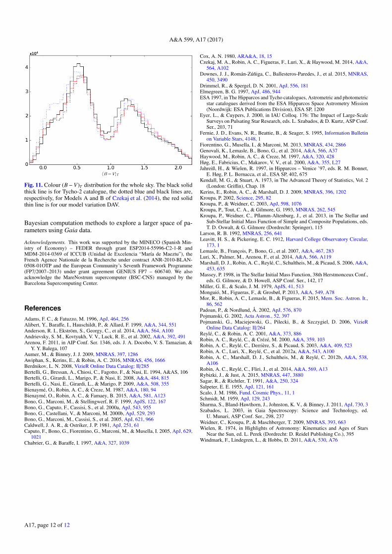
For completeness, in Fig. 11 we compare the (B−V)T colourdistribution for the whole sky Tycho-2 data with our best fitModel variant (DAV) implemented here. We note how the fit ofour model with the whole sky young population in the blue peakof the (B − V) histogram has significantly improved.

6. The IMF in the solar neighbourhood

All methods and data evaluated in the previous section pointtowards the Kroupa-Haywood IMF as the one that best fitsCepheids and Tycho-2 data. This IMF is described with a sim-plified analytical form with three truncated power laws. Usingfield stars and Cepheids, our fits point towards a slope of aboutα = 3.2 at intermediate masses, and excludes the flatter valuesof α = 2.35 of Salpeter IMF. We now want to discuss the scopeof these results both in terms of star formation environment andtime evolution in the Galactic disc. Our results were obtainedusing Galactic Cepheids at all Galactic longitudes located up to≈2 kpc from the Sun. Thus, the derived IMF reflects the massdistribution of the formation episodes that took place in the last200 Myr (upper limit of the Cepheid age) over this region. OurIMF should be understood as a composite IMF, as described inKroupa et al. (2013), one of the best references and review inthis field recently published. Instead of being an IMF derivedfrom an individual cluster or association, our IMF is the sum ofall stellar IMFs from the star formation episodes in the local thindisc environment.

The comparison of our results (α = 3.2) with those in theliterature is complex. To begin with, studies using clusters andOB associations (e.g. Massey 1998) show that, for stars moremassive than the Sun, the IMF can be well approximated by asingle power-law function with the Salpeter index α = 2.35.As mentioned in Kroupa & Weidner (2003), there is a discrep-ancy between the slope of the IMF obtained using field stars(αfield) and the slope of the IMF obtained from stars belong-ing to a cluster (αcluster). This discrepancy (αfield > αcluster) canbe explained by the fact that low mass clusters are more abun-dant than the most massive clusters, then the contribution of thelow mass clusters to the field stars is higher. The abundant lowmass clusters do not have massive stars, while the rare massiveclusters do, and this leads to a steepening of the composite IMF(αfield > αcluster), which is a sum of all the IMFs in all the clus-ters that spawn the Galactic field population (Kroupa & Weidner2003).

Several other studies have derived the IMF using field stars.We should mention the classical work of Scalo (1986) who de-rived a slope of α = 2.7 for M > 1 M�. To compare studies withour results one has to keep in mind that the complexity growsowing to the different ingredients assumed in each case. Criticalparameters such as the SFH, the mass-luminosity relation, theage of the disc, the accuracy in stellar distances, the stellar evo-lutionary models, or the corrections owing to multiple systems,among others, play a significant role. Kroupa et al. (1993), oneof the most referenced works, derived a slope of α = 2.7±0.4 ex-plicitly applying a correction for the unresolved multiple stellarsystems mostly for late-type stars. The effects of the unresolvedmultiple systems on the derivation of the IMF are also discussedin Sagar & Richtler (1991), Kroupa & Weidner 2003 and, for thehigh masses, in Weidner et al. (2009). We want to emphasize thatthe binary treatment performed here (see Sects. 2.1 and 2.2) en-ables us to specifically take into account the angular resolution ofthe catalogues used, thus the treatment of the unresolved systemsis rigorous and its effects are implicitly accounted for. More infavour of our IMF at intermediate masses is its consistency withthe observed stellar density at Sun position and with the Galac-tic rotation curve of Caldwell & Ostriker (1981), all fitted insidethe BGM in a consistent scenario that incorporates dynamicalconstraints (see Sect. 2.4).

To finalize, we cite the recent work of Rybizki & Just (2015).These authors, also using a population synthesis model as a toolfor the derivation of the IMF, obtained a slope of α = 3.02for supersolar masses, which is only slightly flatter than ourvalue. The strength of their method is their combined use of N-body simulations, Galaxia code (based on BGM as default, seeSharma et al. 2011), and Markov chain Monte Carlo techniquesto explore the full parameter space. To conclude, Haywood et al.(1997), Rybizki & Just (2015) and the present work point to-wards a slope of the field stars IMF of about α ≈ 3 at inter-mediate masses.

7. Conclusions

Three different statistical methods have been used to search forthe best IMF that simultaneously fits both the Galactic classi-cal Cepheids and the whole sky Tycho-2 data. All methods arein agreement with the Kroupa-Haywood IMF (Table 3) with aslope of α = 3.2 for intermediate masses. Using both field starsand Galactic classical Cepheids, we have found an IMF thatis steeper than the canonical stellar IMF for the intermediatemasses, both in associations and young clusters. This result isconsistent with the predictions of the Integrated Galactic IMF

A17, page 10 of 12

R. Mor et al.: Constraining the IMF using Galactic Cepheids

Fig. 10. Full 2D posterior probability distribution function. The white stripe shows the tolerance interval region. The plot is for the three cases inFig. 6 that needs a disambiguation: top left panel: DM; top right panel: DBV (different local density); bottom panel: DAV (best fit model withnew scale length). Note here how DM and DAV are almost completely inside the tolerance region, while DBV is half out. DM has an ≈85% ofprobability to have the same observed Cepheid fraction as the Milky Way up to magnitude V = 11, while DBV is just in the ≈50%.

(IGIMF). The three statistical methods considered here showthat a constant SFH is not in agreement with the observationaldata, thus supporting the star formation history as decreasing intime in the Galactic thin disc.

For the first time, we use the BGM to characterize theyoung population of classical Cepheids and use the most up-dated boundaries of the Instability Strip. The BGM enablesus to properly place the stellar evolutionary models in thecontext of the Milky Way evolution modelling. The BGM isnow capable of providing mass and age distributions of classi-cal Cepheids. We have used the most complete catalogues of

Galactic classical Cepheids to confirm these objects as good trac-ers of the intermediate-mass population when constraining theIMF.

The updated BGM population synthesis model inferred bythe Cepheid analysis and undertaken in the present work rep-resents an improvement on the fit with Tycho-2 data, comparedwith Czekaj et al. (2014). With Gaia, thousands of Galactic clas-sical Cepheids will be detected, and the BGM is now ready forthe scientific exploitation of these upcoming extremely accuratedata. In a future study, we aim to consider a non-parametric IMFunlinked from any imposed analytical form and use approximate

A17, page 11 of 12

A&A 599, A17 (2017)

Fig. 11. Colour (B− V)T distribution for the whole sky. The black solidthick line is for Tycho-2 catalogue, the dotted blue and black lines are,respectively, for Models A and B of Czekaj et al. (2014), the red solidthin line is for our model variation DAV.

Bayesian computation methods to explore a larger space of pa-rameters using Gaia data.

Acknowledgements. This work was supported by the MINECO (Spanish Min-istry of Economy) – FEDER through grant ESP2014-55996-C2-1-R andMDM-2014-0369 of ICCUB (Unidad de Excelencia “María de Maeztu”), theFrench Agence Nationale de la Recherche under contract ANR-2010-BLAN-0508-01OTP and the European Community’s Seventh Framework Programme(FP7/2007–2013) under grant agreement GENIUS FP7 – 606740. We alsoacknowledge the MareNostrum supercomputer (BSC-CNS) managed by theBarcelona Supercomputing Center.

ReferencesAdams, F. C., & Fatuzzo, M. 1996, ApJ, 464, 256Alibert, Y., Baraffe, I., Hauschildt, P., & Allard, F. 1999, A&A, 344, 551Anderson, R. I., Ekström, S., Georgy, C., et al. 2014, A&A, 564, A100Andrievsky, S. M., Kovtyukh, V. V., Luck, R. E., et al. 2002, A&A, 392, 491Arenou, F. 2011, in AIP Conf. Ser. 1346, eds. J. A. Docobo, V. S. Tamazian, &

Y. Y. Balega, 107Aumer, M., & Binney, J. J. 2009, MNRAS, 397, 1286Awiphan, S., Kerins, E., & Robin, A. C. 2016, MNRAS, 456, 1666Berdnikov, L. N. 2008, VizieR Online Data Catalog: II/285Bertelli, G., Bressan, A., Chiosi, C., Fagotto, F., & Nasi, E. 1994, A&AS, 106Bertelli, G., Girardi, L., Marigo, P., & Nasi, E. 2008, A&A, 484, 815Bertelli, G., Nasi, E., Girardi, L., & Marigo, P. 2009, A&A, 508, 355Bienaymé, O., Robin, A. C., & Creze, M. 1987, A&A, 180, 94Bienaymé, O., Robin, A. C., & Famaey, B. 2015, A&A, 581, A123Bono, G., Marconi, M., & Stellingwerf, R. F. 1999, ApJS, 122, 167Bono, G., Caputo, F., Cassisi, S., et al. 2000a, ApJ, 543, 955Bono, G., Castellani, V., & Marconi, M. 2000b, ApJ, 529, 293Bono, G., Marconi, M., Cassisi, S., et al. 2005, ApJ, 621, 966Caldwell, J. A. R., & Ostriker, J. P. 1981, ApJ, 251, 61Caputo, F., Bono, G., Fiorentino, G., Marconi, M., & Musella, I. 2005, ApJ, 629,

1021Chabrier, G., & Baraffe, I. 1997, A&A, 327, 1039

Cox, A. N. 1980, ARA&A, 18, 15Czekaj, M. A., Robin, A. C., Figueras, F., Luri, X., & Haywood, M. 2014, A&A,

564, A102Downes, J. J., Román-Zúñiga, C., Ballesteros-Paredes, J., et al. 2015, MNRAS,

450, 3490Drimmel, R., & Spergel, D. N. 2001, ApJ, 556, 181Elmegreen, B. G. 1997, ApJ, 486, 944ESA 1997, in The Hipparcos and Tycho catalogues, Astrometric and photometric

star catalogues derived from the ESA Hipparcos Space Astrometry Mission(Noordwijk: ESA Publications Division), ESA SP, 1200

Eyer, L., & Cuypers, J. 2000, in IAU Colloq. 176: The Impact of Large-ScaleSurveys on Pulsating Star Research, eds. L. Szabados, & D. Kurtz, ASP Conf.Ser., 203, 71

Fernie, J. D., Evans, N. R., Beattie, B., & Seager, S. 1995, Information Bulletinon Variable Stars, 4148, 1

Fiorentino, G., Musella, I., & Marconi, M. 2013, MNRAS, 434, 2866Genovali, K., Lemasle, B., Bono, G., et al. 2014, A&A, 566, A37Haywood, M., Robin, A. C., & Creze, M. 1997, A&A, 320, 428Høg, E., Fabricius, C., Makarov, V. V., et al. 2000, A&A, 355, L27Jahreiß, H., & Wielen, R. 1997, in Hipparcos – Venice ’97, eds. R. M. Bonnet,

E. Høg, P. L. Bernacca, et al., ESA SP, 402, 675Kendall, M. G., & Stuart, A. 1973, in The Advanced Theory of Statistics, Vol. 2

(London: Griffin), Chap. 18Kerins, E., Robin, A. C., & Marshall, D. J. 2009, MNRAS, 396, 1202Kroupa, P. 2002, Science, 295, 82Kroupa, P., & Weidner, C. 2003, ApJ, 598, 1076Kroupa, P., Tout, C. A., & Gilmore, G. 1993, MNRAS, 262, 545Kroupa, P., Weidner, C., Pflamm-Altenburg, J., et al. 2013, in The Stellar and

Sub-Stellar Initial Mass Function of Simple and Composite Populations, eds.T. D. Oswalt, & G. Gilmore (Dordrecht: Springer), 115

Larson, R. B. 1992, MNRAS, 256, 641Leavitt, H. S., & Pickering, E. C. 1912, Harvard College Observatory Circular,

173, 1Lemasle, B., François, P., Bono, G., et al. 2007, A&A, 467, 283Luri, X., Palmer, M., Arenou, F., et al. 2014, A&A, 566, A119Marshall, D. J., Robin, A. C., Reylé, C., Schultheis, M., & Picaud, S. 2006, A&A,

453, 635Massey, P. 1998, in The Stellar Initial Mass Function, 38th Herstmonceux Conf.,

eds. G. Gilmore, & D. Howell, ASP Conf. Ser., 142, 17Miller, G. E., & Scalo, J. M. 1979, ApJS, 41, 513Monguió, M., Figueras, F., & Grosbøl, P. 2013, A&A, 549, A78Mor, R., Robin, A. C., Lemasle, B., & Figueras, F. 2015, Mem. Soc. Astron. It.,

86, 562Padoan, P., & Nordlund, Å. 2002, ApJ, 576, 870Pojmanski, G. 2002, Acta Astron., 52, 397Pojmanski, G., Maciejewski, G., Pilecki, B., & Szczygiel, D. 2006, VizieR

Online Data Catalog: II/264Reylé, C., & Robin, A. C. 2001, A&A, 373, 886Robin, A. C., Reylé, C., & Crézé, M. 2000, A&A, 359, 103Robin, A. C., Reylé, C., Derrière, S., & Picaud, S. 2003, A&A, 409, 523Robin, A. C., Luri, X., Reylé, C., et al. 2012a, A&A, 543, A100Robin, A. C., Marshall, D. J., Schultheis, M., & Reylé, C. 2012b, A&A, 538,

A106Robin, A. C., Reylé, C., Fliri, J., et al. 2014, A&A, 569, A13Rybizki, J., & Just, A. 2015, MNRAS, 447, 3880Sagar, R., & Richtler, T. 1991, A&A, 250, 324Salpeter, E. E. 1955, ApJ, 121, 161Scalo, J. M. 1986, Fund. Cosmic Phys., 11, 1Schmidt, M. 1959, ApJ, 129, 243Sharma, S., Bland-Hawthorn, J., Johnston, K. V., & Binney, J. 2011, ApJ, 730, 3Szabados, L. 2003, in Gaia Spectroscopy: Science and Technology, ed.

U. Munari, ASP Conf. Ser., 298, 237Weidner, C., Kroupa, P., & Maschberger, T. 2009, MNRAS, 393, 663Wielen, R. 1974, in Highlights of Astronomy: Kinematics and Ages of Stars

Near the Sun, ed. L. Perek (Dordrecht: D. Reidel Publishing Co.), 395Windmark, F., Lindegren, L., & Hobbs, D. 2011, A&A, 530, A76

A17, page 12 of 12