constant partying: growing and handling trees with constant fits

Constant Partying: Growing and Handling Trees

with Constant Fits

Torsten Hothorn

Universitat ZurichAchim Zeileis

Universitat Innsbruck

Abstract

This vignette describes infrastructure for regression and classification trees with simpleconstant fits in each of the terminal nodes. Thus, all observations that are predicted tobe in the same terminal node also receive the same prediction, e.g., a mean for numericresponses or proportions for categorical responses. This class of trees is very common andincludes all traditional tree variants (AID, CHAID, CART, C4.5, FACT, QUEST) andalso more recent approaches like CTree. Trees inferred by any of these algorithms could inprinciple be represented by objects of class “constparty” in partykit that then providesunified methods for printing, plotting, and predicting. Here, we describe how one cancreate “constparty” objects by (a) coercion from other R classes, (b) parsing of XMLdescriptions of trees learned in other software systems, (c) learning a tree using one’s ownalgorithm.

Keywords: recursive partitioning, regression trees, classification trees, decision trees.

1. Classes and methods

This vignette describes the handling of trees with constant fits in the terminal nodes. Thisclass of regression models includes most classical tree algorithms like AID (Morgan and Son-quist 1963), CHAID (Kass 1980), CART (Breiman, Friedman, Olshen, and Stone 1984),FACT (Loh and Vanichsetakul 1988), QUEST (Loh and Shih 1997), C4.5 (Quinlan 1993),CTree (Hothorn, Hornik, and Zeileis 2006) etc. In this class of tree models, one can com-pute simple predictions for new observations, such as the conditional mean in a regressionsetup, from the responses of those learning sample observations in the same terminal node.Therefore, such predictions can easily be computed if the following pieces of information areavailable: the observed responses in the learning sample, the terminal node IDs assigned tothe observations in the learning sample, and potentially associated weights (if any).

In partykit it is easy to create a “party” object that contains these pieces of information,yielding a “constparty” object. The technical details of the “party” class are discussed indetail in Section 3.4 of vignette("partykit", package = "partykit"). In addition to theelements required for any “party”, a “constparty” needs to have: variables (fitted) and(response) (and (weights) if applicable) in the fitted data frame along with the terms

for the model. If such a “party” has been created, its properties can be checked and coercedto class “constparty” by the as.constparty() function.

Note that with such a “constparty” object it is possible to compute all kinds of predictionsfrom the subsample in a given terminal node. For example, instead the mean response the

2 Constant Partying: Growing and Handling Trees with Constant Fits

median (or any other quantile) could be employed. Similarly, for a categorical response thepredicted probabilities (i.e., relative frequencies) can be computed or the corresponding modeor a ranking of the levels etc.

In case the full response from the learning sample is not available but only the constant fitfrom each terminal node, then a “constparty” cannot be set up. Specifically, this is thecase for trees saved in the XML format PMML (Predictive Model Markup Language, DataMining Group 2014) that does not provide the full learning sample. To also support suchconstant-fit trees based on simpler information partykit provides the “simpleparty” class.Inspired by the PMML format, this requires that the info of every node in the tree provideslist elements prediction, n, error, and distribution. For classification trees these shouldcontain the following node-specific information: the predicted single predicted factor, thelearning sample size, the misclassification error (in %), and the absolute frequencies of alllevels. For regression trees the contents should be: the predicted mean, the learning samplesize, the error sum of squares, and NULL. The function as.simpleparty() can also coerce“constparty” trees to “simpleparty” trees by computing the above summary statistics fromthe full response associated with each node of the tree.

The remainder of this vignette consists of the following parts: In Section 2 we assume thatthe trees were fitted using some other software (either within or outside of R) and we de-scribe how these models can be coerced to “party” objects using either the “constparty” or“simpleparty” class. Emphasize is given to displaying such trees in textual and graphicalways. Subsequently, in Section 3, we show a simple classification tree algorithm can be easilyimplemented using the partykit tools, yielding a “constparty” object. Section 4 shows howto compute predictions in both scenarios before Section 5 finally gives a brief conclusion.

2. Coercing tree objects

For the illustrations, we use the Titanic data set from package datasets, consisting of fourvariables on each of the 2201 Titanic passengers: gender (male, female), age (child, adult),and class (1st, 2nd, 3rd, or crew) set up as follows:

> data("Titanic", package = "datasets")

> ttnc <- as.data.frame(Titanic)

> ttnc <- ttnc[rep(1:nrow(ttnc), ttnc$Freq), 1:4]

> names(ttnc)[2] <- "Gender"

The response variable describes whether or not the passenger survived the sinking of the ship.

2.1. Coercing rpart objects

We first fit a classification tree by means of the the rpart() function from package rpart

(Therneau and Atkinson 1997) to this data set (make sure to set model = TRUE; otherwisemodel.frame.rpart will return the rpart object and not the data):

> library("rpart")

> (rp <- rpart(Survived ~ ., data = ttnc, model = TRUE))

n= 2201

Torsten Hothorn, Achim Zeileis 3

node), split, n, loss, yval, (yprob)

* denotes terminal node

1) root 2201 711 No (0.6769650 0.3230350)

2) Gender=Male 1731 367 No (0.7879838 0.2120162)

4) Age=Adult 1667 338 No (0.7972406 0.2027594) *

5) Age=Child 64 29 No (0.5468750 0.4531250)

10) Class=3rd 48 13 No (0.7291667 0.2708333) *

11) Class=1st,2nd 16 0 Yes (0.0000000 1.0000000) *

3) Gender=Female 470 126 Yes (0.2680851 0.7319149)

6) Class=3rd 196 90 No (0.5408163 0.4591837) *

7) Class=1st,2nd,Crew 274 20 Yes (0.0729927 0.9270073) *

The “rpart” object rp can be coerced to a “constparty” by as.party(). Internally, thistransforms the tree structure of the “rpart” tree to a “partynode” and combines it with theassociated learning sample as described in Section 1. All of this is done automatically by

> (party_rp <- as.party(rp))

Model formula:

Survived ~ Class + Gender + Age

Fitted party:

[1] root

| [2] Gender in Male

| | [3] Age in Adult: No (n = 1667, err = 20.3%)

| | [4] Age in Child

| | | [5] Class in 3rd: No (n = 48, err = 27.1%)

| | | [6] Class in 1st, 2nd: Yes (n = 16, err = 0.0%)

| [7] Gender in Female

| | [8] Class in 3rd: No (n = 196, err = 45.9%)

| | [9] Class in 1st, 2nd, Crew: Yes (n = 274, err = 7.3%)

Number of inner nodes: 4

Number of terminal nodes: 5

Now, instead of the print method for“rpart”objects the print method for constparty objectscreates a textual display of the tree structure. In a similar way, the corresponding plot()

method produces a graphical representation of this tree, see Figure 1.

By default, the predict() method for “rpart” objects computes conditional class probabili-ties. The same numbers are returned by the predict() method for constparty objects withtype = "prob" argument (see Section 4 for more details):

> all.equal(predict(rp), predict(party_rp, type = "prob"),

+ check.attributes = FALSE)

[1] TRUE


> plot(rp)

> text(rp)

|Gender=a

Age=b

Class=c

Class=c

No

No Yes

No Yes

> plot(party_rp)

Gender

1

Male Female

Age

2

Adult Child

Node 3 (n = 1667)

Yes

No

0

0.2

0.4

0.6

0.8

1

Class

4

3rd 1st, 2nd

Node 5 (n = 48)

Yes

No

0

0.2

0.4

0.6

0.8

1Node 6 (n = 16)

Yes

No

0

0.2

0.4

0.6

0.8

1

Class

7

3rd 1st, 2nd, Crew

Node 8 (n = 196)

Yes

No

0

0.2

0.4

0.6

0.8

1Node 9 (n = 274)

Yes

No

0

0.2

0.4

0.6

0.8

1

Figure 1: “rpart” tree of Titanic data plotted using rpart (top) and partykit (bottom) in-frastructure.


Predictions are computed based on the fitted slot of a “constparty” object

> str(fitted(party_rp))

'data.frame': 2201 obs. of 2 variables:

$ (fitted) : int 5 5 5 5 5 5 5 5 5 5 ...

$ (response): Factor w/ 2 levels "No","Yes": 1 1 1 1 1 1 1 1 1 1 ...

which contains the terminal node numbers and the response for each of the training samples.So, the conditional class probabilities for each terminal node can be computed via

> prop.table(do.call("table", fitted(party_rp)), 1)

(response)

(fitted) No Yes

3 0.7972406 0.2027594

5 0.7291667 0.2708333

6 0.0000000 1.0000000

8 0.5408163 0.4591837

9 0.0729927 0.9270073

Optionally, weights can be stored in the fitted slot as well.

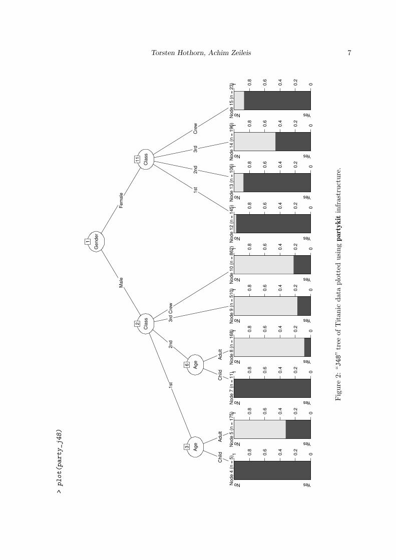
2.2. Coercing J48 objects

The RWeka package (Hornik, Buchta, and Zeileis 2009) provides an interface to the Weka

machine learning library and we can use the J48() function to fit a J4.8 tree to the Titanicdata

> if (require("RWeka")) {

+ j48 <- J48(Survived ~ ., data = ttnc)

+ } else {

+ j48 <- rpart(Survived ~ ., data = ttnc)

+ }

> print(j48)

J48 pruned tree

------------------

Gender = Male

| Class = 1st

| | Age = Child: Yes (5.0)

| | Age = Adult: No (175.0/57.0)

| Class = 2nd

| | Age = Child: Yes (11.0)

| | Age = Adult: No (168.0/14.0)

| Class = 3rd: No (510.0/88.0)


| Class = Crew: No (862.0/192.0)

Gender = Female

| Class = 1st: Yes (145.0/4.0)

| Class = 2nd: Yes (106.0/13.0)

| Class = 3rd: No (196.0/90.0)

| Class = Crew: Yes (23.0/3.0)

Number of Leaves : 10

Size of the tree : 15

This object can be coerced to a “party” object using

> (party_j48 <- as.party(j48))

Model formula:


Fitted party:

[1] root


| | [3] Class in 1st

| | | [4] Age in Child: Yes (n = 5, err = 0.0%)

| | | [5] Age in Adult: No (n = 175, err = 32.6%)

| | [6] Class in 2nd




| | [10] Class in Crew: No (n = 862, err = 22.3%)


| | [12] Class in 1st: Yes (n = 145, err = 2.8%)

| | [13] Class in 2nd: Yes (n = 106, err = 12.3%)


| | [15] Class in Crew: Yes (n = 23, err = 13.0%)



and, again, the print method from the partykit package creates a textual display. Note that,unlike the “rpart” trees, this tree includes multiway splits. The plot() method draws thistree, see Figure 2.

The conditional class probabilities computed by the predict() methods implemented inpackages RWeka and partykit are equivalent:

> all.equal(predict(j48, type = "prob"), predict(party_j48, type = "prob"),


Torsten Hothorn, Achim Zeileis 7>plot(party_j48)

Ge

nd

er

1

Ma

leF

em

ale

Cla

ss

2

1st

2n

d3

rdC

rew

Ag

e

3

Ch

ildA

du

lt

No

de

4 (

n =

5)

YesNo

00.2

0.4

0.6

0.8

1N

od

e 5

(n

= 1

75

)

YesNo

00.2

0.4

0.6

0.8

1

Ag

e

6

Ch

ildA

du

lt

No

de

7 (

n =

11

)

YesNo

00.2

0.4

0.6

0.8

1N

od

e 8

(n

= 1

68

)

YesNo

00.2

0.4

0.6

0.8

1N

od

e 9

(n

= 5

10

)

YesNo

00.2

0.4

0.6

0.8

1N

od

e 1

0 (

n =

86

2)

YesNo

00.2

0.4

0.6

0.8

1

Cla

ss

11

1st

2n

d3

rdC

rew

No

de

12

(n

= 1

45

)

YesNo

00.2

0.4

0.6

0.8

1N

od

e 1

3 (

n =

10

6)

YesNo

00.2

0.4

0.6

0.8

1N

od

e 1

4 (

n =

19

6)

YesNo

00.2

0.4

0.6

0.8

1N

od

e 1

5 (

n =

23

)

YesNo

00.2

0.4

0.6

0.8

1

Figure

2:“J48”tree

ofTitan

icdataplotted

usingpartykitinfrastructure.


[1] TRUE

In addition to J48() RWeka provides several other tree learners, e.g., M5P() implementingM5’ and LMT() implementing logistic model trees, respectively. These can also be coercedusing as.party(). However, as these are not constant-fit trees this yields plain “party” treeswith some character information stored in the info slot.

2.3. Importing trees from PMML files

The previous two examples showed how trees learned by other R packages can be handled ina unified way using partykit. Additionally, partykit can also be used to import trees fromany other software package that supports the PMML (Predictive Model Markup Language)format.

As an example, we used SPSS to fit a QUEST tree to the Titanic data and exported this fromSPSS in PMML format. This file is shipped along with the partykit package and we can readit as follows:

> ttnc_pmml <- file.path(system.file("pmml", package = "partykit"),

+ "ttnc.pmml")

> (ttnc_quest <- pmmlTreeModel(ttnc_pmml))

Model formula:

Survived ~ Gender + Class + Age

Fitted party:

[1] root


| | [3] Class in 3rd, Crew: Yes (n = 219, err = 49.8%)

| | [4] Class in 1st, 2nd

| | | [5] Class in 2nd: Yes (n = 106, err = 12.3%)

| | | [6] Class in 1st: Yes (n = 145, err = 2.8%)


| | [8] Class in 3rd, 2nd, Crew

| | | [9] Age in Child: No (n = 59, err = 40.7%)

| | | [10] Age in Adult

| | | | [11] Class in 3rd, Crew

| | | | | [12] Class in Crew: No (n = 862, err = 22.3%)

| | | | | [13] Class in 3rd: No (n = 462, err = 16.2%)

| | | | [14] Class in 2nd: No (n = 168, err = 8.3%)

| | [15] Class in 1st: No (n = 180, err = 34.4%)



The object ttnc_quest is of class “simpleparty” and the corresponding graphical display isshown in Figure 3. As explained in Section 1, the full learning data are not part of the PMML


> plot(ttnc_quest)

Gender

1

Female Male

Class

2

3rd, Crew 1st, 2nd

Yes

(n = 219, err = 49.8%)

3

Class

4

2nd 1st

Yes

(n = 106, err = 12.3%)

5

Yes

(n = 145, err = 2.8%)

6

Class

7

3rd, 2nd, Crew 1st

Age

8

Child Adult

No

(n = 59, err = 40.7%)

9

Class

10

3rd, Crew 2nd

Class

11

Crew 3rd

No

(n = 862, err = 22.3%)

12

No

(n = 462, err = 16.2%)

13

No

(n = 168, err = 8.3%)

14

No

(n = 180, err = 34.4%)

15

Figure 3: QUEST tree for Titanic data, fitted using SPSS and exported via PMML.

description and hence one can only obtain and display the summarized information providedby PMML.

In this particular case, however, we have the learning data available in R because we had ex-ported the data from R to begin with. Hence, for this tree we can augment the“simpleparty”with the full learning sample to create a “constparty”. As SPSS had reordered some factorlevels we need to carry out this reordering as well”

> ttnc2 <- ttnc[, names(ttnc_quest$data)]

> for(n in names(ttnc2)) {

+ if(is.factor(ttnc2[[n]])) ttnc2[[n]] <- factor(

+ ttnc2[[n]], levels = levels(ttnc_quest$data[[n]]))

+ }

Using this data all information for a “constparty” can be easily computed:

> ttnc_quest2 <- party(ttnc_quest$node,

+ data = ttnc2,

+ fitted = data.frame(

+ "(fitted)" = predict(ttnc_quest, ttnc2, type = "node"),

+ "(response)" = ttnc2$Survived,

+ check.names = FALSE),

+ terms = terms(Survived ~ ., data = ttnc2)

+ )

> ttnc_quest2 <- as.constparty(ttnc_quest2)

This object is plotted in Figure 4.


> plot(ttnc_quest2)

Gender

1

Female Male

Class

2

3rd, Crew 1st, 2nd

Node 3 (n = 219)

Ye

sN

o

0

0.2

0.4

0.6

0.8

1

Class

4

2nd 1st

Node 5 (n = 106)

Ye

sN

o

0

0.2

0.4

0.6

0.8

1Node 6 (n = 145)

Ye

sN

o

0

0.2

0.4

0.6

0.8

1

Class

7

3rd, 2nd, Crew 1st

Age

8

Child Adult

Node 9 (n = 59)

Ye

sN

o

0

0.2

0.4

0.6

0.8

1

Class

10

3rd, Crew 2nd

Class

11

Crew 3rd

Node 12 (n = 862)

Ye

sN

o

0

0.2

0.4

0.6

0.8

1Node 13 (n = 462)

Ye

sN

o

0

0.2

0.4

0.6

0.8

1Node 14 (n = 168)

Ye

sN

o

0

0.2

0.4

0.6

0.8

1Node 15 (n = 180)

Ye

sN

o

0

0.2

0.4

0.6

0.8

1

Figure 4: QUEST tree for Titanic data, fitted using SPSS, exported via PMML, and trans-formed into a “constparty” object.

Furthermore, we briefly point out that there is also the R package pmml (Williams, Jena, Hah-sler, Zementis Inc., Ishwaran, Kogalur, and Guha 2014), part of the rattle project (Williams2011), that allows to export PMML files for rpart trees from R. For example, for the “rpart”tree for the Titanic data:

> library("pmml")

> tfile <- tempfile()

> write(toString(pmml(rp)), file = tfile)

Then, we can simply read this file and inspect the resulting tree

> (party_pmml <- pmmlTreeModel(tfile))

Model formula:


Fitted party:

[1] root


| | [3] Age in Adult: No (n = 1667, err = 20.3%)

| | [4] Age in Child


| | | [5] Class in 3rd: No (n = 48, err = 27.1%)

| | | [6] Class in 1st, 2nd: Yes (n = 16, err = 0.0%)






> all.equal(predict(party_rp, newdata = ttnc, type = "prob"),

+ predict(party_pmml, newdata = ttnc, type = "prob"),


[1] TRUE

Further example PMML files created with rattle are the Data Mining Group web page, e.g.,http://www.dmg.org/pmml_examples/rattle_pmml_examples/AuditTree.xml or http://www.dmg.org/pmml_examples/rattle_pmml_examples/IrisTree.xml.

3. Growing a simple classification tree

Although the partykit package offers an extensive toolbox for handling trees along with im-plementations of various tree algorithms, it does not offer unified infrastructure for growing

trees. However, once you know how to estimate splits from data, it is fairly straightforwardto implement trees. Consider a very simple CHAID-style algorithm (in fact so simple thatwe would advise not to use it for any real application). We assume that both response andexplanatory variables are factors, as for the Titanic data set. First we determine the bestexplanatory variable by means of a global χ2 test, i.e., splitting up the response into all levelsof each explanatory variable. Then, for the selected explanatory variable we search for thebinary best split by means of χ2 tests, i.e., we cycle through all potential split points andassess the quality of the split by comparing the distributions of the response in the so-definedtwo groups. In both cases, we select the split variable/point with lowest p-value from the χ

2

test, however, only if the global test is significant at Bonferroni-corrected level α = 0.01.

This strategy can be implemented based on the data (response and explanatory variables)and some case weights as follows (response is just the name of the response and data is adata frame with all variables):

> findsplit <- function(response, data, weights, alpha = 0.01) {

+

+ ## extract response values from data

+ y <- factor(rep(data[[response]], weights))

+

+ ## perform chi-squared test of y vs. x

+ mychisqtest <- function(x) {

+ x <- factor(x)

+ if(length(levels(x)) < 2) return(NA)

http://www.dmg.org/pmml_examples/rattle_pmml_examples/AuditTree.xml

http://www.dmg.org/pmml_examples/rattle_pmml_examples/IrisTree.xml

http://www.dmg.org/pmml_examples/rattle_pmml_examples/IrisTree.xml


+ ct <- suppressWarnings(chisq.test(table(y, x), correct = FALSE))

+ pchisq(ct$statistic, ct$parameter, log = TRUE, lower.tail = FALSE)

+ }

+ xselect <- which(names(data) != response)

+ logp <- sapply(xselect, function(i) mychisqtest(rep(data[[i]], weights)))

+ names(logp) <- names(data)[xselect]

+

+ ## Bonferroni-adjusted p-value small enough?

+ if(all(is.na(logp))) return(NULL)

+ minp <- exp(min(logp, na.rm = TRUE))

+ minp <- 1 - (1 - minp)^sum(!is.na(logp))

+ if(minp > alpha) return(NULL)

+

+ ## for selected variable, search for split minimizing p-value

+ xselect <- xselect[which.min(logp)]

+ x <- rep(data[[xselect]], weights)

+

+ ## set up all possible splits in two kid nodes

+ lev <- levels(x[drop = TRUE])

+ if(length(lev) == 2) {

+ splitpoint <- lev[1]

+ } else {

+ comb <- do.call("c", lapply(1:(length(lev) - 2),

+ function(x) combn(lev, x, simplify = FALSE)))

+ xlogp <- sapply(comb, function(q) mychisqtest(x %in% q))

+ splitpoint <- comb[[which.min(xlogp)]]

+ }

+

+ ## split into two groups (setting groups that do not occur to NA)

+ splitindex <- !(levels(data[[xselect]]) %in% splitpoint)

+ splitindex[!(levels(data[[xselect]]) %in% lev)] <- NA_integer_

+ splitindex <- splitindex - min(splitindex, na.rm = TRUE) + 1L

+

+ ## return split as partysplit object

+ return(partysplit(varid = as.integer(xselect),

+ index = splitindex,

+ info = list(p.value = 1 - (1 - exp(logp))^sum(!is.na(logp)))))

+ }

In order to actually grow a tree on data, we have to set up the recursion for growing a recursive“partynode” structure:

> growtree <- function(id = 1L, response, data, weights, minbucket = 30) {

+

+ ## for less than 30 observations stop here

+ if (sum(weights) < minbucket) return(partynode(id = id))

+


+ ## find best split

+ sp <- findsplit(response, data, weights)

+ ## no split found, stop here

+ if (is.null(sp)) return(partynode(id = id))

+

+ ## actually split the data

+ kidids <- kidids_split(sp, data = data)

+

+ ## set up all daugther nodes

+ kids <- vector(mode = "list", length = max(kidids, na.rm = TRUE))

+ for (kidid in 1:length(kids)) {

+ ## select observations for current node

+ w <- weights

+ w[kidids != kidid] <- 0

+ ## get next node id

+ if (kidid > 1) {

+ myid <- max(nodeids(kids[[kidid - 1]]))

+ } else {

+ myid <- id

+ }

+ ## start recursion on this daugther node

+ kids[[kidid]] <- growtree(id = as.integer(myid + 1), response, data, w)

+ }

+

+ ## return nodes

+ return(partynode(id = as.integer(id), split = sp, kids = kids,

+ info = list(p.value = min(info_split(sp)$p.value, na.rm = TRUE))))

+ }

A very rough sketch of a formula-based user-interface sets-up the data and calls growtree():

> mytree <- function(formula, data, weights = NULL) {

+

+ ## name of the response variable

+ response <- all.vars(formula)[1]

+ ## data without missing values, response comes last

+ data <- data[complete.cases(data), c(all.vars(formula)[-1], response)]

+ ## data is factors only

+ stopifnot(all(sapply(data, is.factor)))

+

+ if (is.null(weights)) weights <- rep(1L, nrow(data))

+ ## weights are case weights, i.e., integers

+ stopifnot(length(weights) == nrow(data) &

+ max(abs(weights - floor(weights))) < .Machine$double.eps)

+

+ ## grow tree

+ nodes <- growtree(id = 1L, response, data, weights)


+

+ ## compute terminal node number for each observation

+ fitted <- fitted_node(nodes, data = data)

+ ## return rich constparty object

+ ret <- party(nodes, data = data,

+ fitted = data.frame("(fitted)" = fitted,

+ "(response)" = data[[response]],

+ "(weights)" = weights,

+ check.names = FALSE),

+ terms = terms(formula))

+ as.constparty(ret)

+ }

The call to the constructor party() sets-up a “party” object with the tree structure con-tained in nodes, the training samples in data and the corresponding terms object. Class“constparty” inherits all slots from class “party” and has an additional fitted slot for stor-ing the terminal node numbers for each sample in the training data, the response variable(s)and case weights. The fitted slot is a “data.frame” containing three variables: The fittedterminal node identifiers "(fitted)", an integer vector of the same length as data; the re-sponse variables "(response)" as a vector (or data.frame for multivariate responses) withthe same number of observations; and optionally a vector of weights "(weights)". The addi-tional fitted slot allows to compute arbitrary summary measures for each terminal node bysimply subsetting the "(response)" and "(weights)" slots by "(fitted)" before comput-ing (weighted) means, medians, empirical cumulative distribution functions, Kaplan-Meierestimates or whatever summary statistic might be appropriate for a certain response. Theprint(), plot(), and predict() methods for class“constparty”work this way with suitabledefaults for the summary statistics depending on the class of the response(s).

We now can fit this tree to the Titanic data; the print() method provides us with a firstoverview on the resulting model

> (myttnc <- mytree(Survived ~ Class + Age + Gender, data = ttnc))

Model formula:

Survived ~ Class + Age + Gender

Fitted party:

[1] root


| | [3] Class in 1st



| | [6] Class in 2nd, 3rd, Crew

| | | [7] Age in Child

| | | | [8] Class in 2nd: Yes (n = 11, err = 0.0%)

| | | | [9] Class in 3rd: No (n = 48, err = 27.1%)

| | | [10] Age in Adult

| | | | [11] Class in Crew: No (n = 862, err = 22.3%)


Gender

p < 0.001

1

Male Female

Class

p < 0.001

2

1st 2nd, 3rd, Crew

Age

p = 0.002

3

Child Adult

Node 4 (n = 5)

Ye

sN

o

0

0.2

0.4

0.6

0.8

1Node 5 (n = 175)

Ye

sN

o

0

0.2

0.4

0.6

0.8

1

Age

p < 0.001

6

Child Adult

Class

p < 0.001

7

2nd 3rd

Node 8 (n = 11)

Ye

sN

o

0

0.2

0.4

0.6

0.8

1Node 9 (n = 48)

Ye

sN

o

0

0.2

0.4

0.6

0.8

1

Class

p < 0.001

10

Crew 2nd, 3rd

Node 11 (n = 862)

Ye

sN

o

0

0.2

0.4

0.6

0.8

1Node 12 (n = 630)

Ye

sN

o0

0.2

0.4

0.6

0.8

1

Class

p < 0.001

13

3rd 1st, 2nd, Crew

Node 14 (n = 196)

Ye

sN

o

0

0.2

0.4

0.6

0.8

1Node 15 (n = 274)

Ye

sN

o

0

0.2

0.4

0.6

0.8

1

Figure 5: Classification tree fitted by the mytree() function to the ttnc data.

| | | | [12] Class in 2nd, 3rd: No (n = 630, err = 14.1%)






Of course, we can immediately use plot(myttnc) to obtain a graphical representation of thistree, the result is given in Figure 5. The default behavior for trees with categorical responsesis simply inherited from “constparty” and hence we readily obtain bar plots in all terminalnodes.

As the tree is fairly large, we might be interested in pruning the tree to a more reasonable size.For this purpose the partykit package provides the nodeprune() function that can prune backto nodes with selected IDs. As nodeprune() (by design) does not provide a specific pruningcriterion, we need to determine ourselves which nodes to prune. Here, one idea could be toimpose significance at a higher level than the default 10−2 – say 10−5 to obtain a stronglypruned tree. Hence we use nodeapply() to extract the minimal Bonferroni-corrected p-valuefrom all inner nodes:

> nid <- nodeids(myttnc)

> iid <- nid[!(nid %in% nodeids(myttnc, terminal = TRUE))]

> (pval <- unlist(nodeapply(myttnc, ids = iid,

+ FUN = function(n) info_node(n)$p.value)))


Gender

p < 0.001

1

Male Female

Class

p < 0.001

2

1st 2nd, 3rd, Crew

Node 3 (n = 180)

Yes

No

0

0.2

0.4

0.6

0.8

1Node 4 (n = 1747)

Yes

No

0

0.2

0.4

0.6

0.8

1

Class

p < 0.001

5

3rd 1st, 2nd, Crew

Node 6 (n = 0)

Yes

No

0

0.2

0.4

0.6

0.8

1Node 7 (n = 274)

Yes

No

0

0.2

0.4

0.6

0.8

1

Figure 6: Pruned classification tree fitted by the mytree() function to the ttnc data.

1 2 3 6 7

0.000000e+00 2.965383e-06 1.756527e-03 6.933623e-05 8.975754e-06

10 13

2.992870e-05 0.000000e+00

Then, the pruning of the nodes with the larger p-values can be simply carried out by

> myttnc2 <- nodeprune(myttnc, ids = iid[pval > 1e-5])

The corresponding visualization is shown in Figure 6.

The accuracy of the tree built using the default options could be assessed by the bootstrap,for example. Here, we want to compare our tree for the Titanic survivor data with a simplelogistic regression model. First, we fit this simple GLM and compute the (in-sample) log-likelihood:

> logLik(glm(Survived ~ Class + Age + Gender, data = ttnc,

+ family = binomial()))

'log Lik.' -1105.031 (df=6)

For our tree, we set-up 25 bootstrap samples

> bs <- rmultinom(25, nrow(ttnc), rep(1, nrow(ttnc)) / nrow(ttnc))

and implement the log-likelihood of a binomal model

> bloglik <- function(prob, weights)

+ sum(weights * dbinom(ttnc$Survived == "Yes", size = 1,

+ prob[,"Yes"], log = TRUE))


What remains to be done is to iterate over all bootstrap samples, to refit the tree on thebootstrap sample and to evaluate the log-likelihood on the out-of-bootstrap samples based onthe trees’ predictions (details on how to compute predictions are given in the next section):

> f <- function(w) {

+ tr <- mytree(Survived ~ Class + Age + Gender, data = ttnc, weights = w)

+ bloglik(predict(tr, newdata = ttnc, type = "prob"), as.numeric(w == 0))

+ }

> apply(bs, 2, f)

[1] -390.2268 -410.8696 -377.7492 -416.7790 -396.5327 -383.9575

[7] -389.4972 -405.8401 -379.9248 -384.7071 -381.1303 -394.8712

[13] -409.8711 -385.3753 -396.2723 -385.6372 -408.9187 -412.4585

[19] -401.3972 -403.0548 -406.7881 -389.8507 -408.0418 -392.1441

[25] -389.4687

We see that the in-sample log-likelihood of the linear logistic regression model is much smallerthan the out-of-sample log-likelihood found for our tree and thus we can conclude that ourtree-based approach fits data the better than the linear model.

4. Predictions

As argued in Section 1 arbitrary types of predictions can be computed from “constparty”objects because the full empirical distribution of the response in the learning sample nodesis available. All of these can be easily computed in the predict() method for “constparty”objects by supplying a suitable aggregation function. However, as certain types of predic-tions are much more commonly used, these are available even more easily by setting a type

argument.

The prediction type can either be "node", "response", or "prob" (see Table 1). The ideais that "response" always returns a prediction of the same class as the original responseand "prob" returns some object that characterizes the entire empirical distribution. Hence,for different response classes, different types of predictions are produced, see Table 1 for anoverview. Additionally, for “numeric” responses type = "quantile" and type = "density"

is available. By default, these return functions for computing predicted quantiles and proba-bility densities, respectively, but optionally these functions can be directly evaluated at givenvalues and then return a vector/matrix.

Here, we illustrate all different predictions for all possible combinations of the explanatoryfactor levels.

Response class type = "node" type = "response" type = "prob"

“factor” terminal node number majority class class probabilities“numeric” terminal node number mean ECDF“Surv” terminal node number median survival time Kaplan-Meier

Table 1: Overview on type of predictions computed by the predict() method for“constparty” objects. For multivariate responses, combinations thereof are returned.


> nttnc <- expand.grid(Class = levels(ttnc$Class),

+ Gender = levels(ttnc$Gender), Age = levels(ttnc$Age))

> nttnc

Class Gender Age

1 1st Male Child

2 2nd Male Child

3 3rd Male Child

4 Crew Male Child

5 1st Female Child

6 2nd Female Child

7 3rd Female Child

8 Crew Female Child

9 1st Male Adult

10 2nd Male Adult

11 3rd Male Adult

12 Crew Male Adult

13 1st Female Adult

14 2nd Female Adult

15 3rd Female Adult

16 Crew Female Adult

The corresponding predicted nodes, modes, and probability distributions are:

> predict(myttnc, newdata = nttnc, type = "node")

1 2 3 4 5 6 7 8 9 10 11 12 13 14 15 16

4 8 9 9 15 15 14 15 5 12 12 11 15 15 14 15

> predict(myttnc, newdata = nttnc, type = "response")

1 2 3 4 5 6 7 8 9 10 11 12 13 14 15 16

Yes Yes No Yes Yes Yes No Yes No No No No Yes Yes No Yes

Levels: No Yes

> predict(myttnc, newdata = nttnc, type = "prob")

No Yes

1 0.0000000 1.0000000

2 0.0000000 1.0000000

3 0.7291667 0.2708333

4 0.0000000 1.0000000

5 0.0729927 0.9270073

6 0.0729927 0.9270073

7 0.5408163 0.4591837

8 0.0729927 0.9270073


9 0.6742857 0.3257143

10 0.8587302 0.1412698

11 0.8587302 0.1412698

12 0.7772622 0.2227378

13 0.0729927 0.9270073

14 0.0729927 0.9270073

15 0.5408163 0.4591837

16 0.0729927 0.9270073

Furthermore, the predict() method features a FUN argument that can be used to computecustomized predictions. If we are, say, interested in the rank of the probabilities for the twoclasses, we can simply specify a function that implements this feature:

> predict(myttnc, newdata = nttnc, FUN = function(y, w)

+ rank(table(rep(y, w))))

No Yes

1 1 2

2 1 2

3 2 1

4 1 2

5 1 2

6 1 2

7 2 1

8 1 2

9 2 1

10 2 1

11 2 1

12 2 1

13 1 2

14 1 2

15 2 1

16 1 2

The user-supplied function FUN takes two arguments, y is the response and w is a vector ofweights (case weights in this situation). Of course, it would have been easier to do these com-putations directly on the conditional class probabilities (type = "prob"), but the approachtaken here for illustration generalizes to situations where this is not possible, especially fornumeric responses.

5. Conclusion

The classes “constparty” and “simpleparty” introduced here can be used to represent treeswith constant fits in the terminal nodes, including most of the traditional tree variants. For anumber of implementations it is possible to convert the resulting trees to one of these classes,thus offering unified methods for handling constant-fit trees. User-extensible methods for


printing and plotting these trees are available. Also, computing non-standard predictions,such as the median or empirical cumulative distribution functions, is easily possible withinthis framework. With the infrastructure provided in partykit it is rather straightforward toimplement a new (or old) tree algorithm and therefore a prototype implementation of fancyideas for improving trees is only a couple lines of R code away.

References

Breiman L, Friedman JH, Olshen RA, Stone CJ (1984). Classification and Regression Trees.Wadsworth, California.

Data Mining Group (2014). “Predictive Model Markup Language.” Version 4.2, URL http:

//www.dmg.org/.

Hornik K, Buchta C, Zeileis A (2009). “Open-Source Machine Learning: R Meets Weka.”Computational Statistics, 24(2), 225–232.

Hothorn T, Hornik K, Zeileis A (2006). “Unbiased Recursive Partitioning: A ConditionalInference Framework.” Journal of Computational and Graphical Statistics, 15(3), 651–674.

Kass GV (1980). “An Exploratory Technique for Investigating Large Quantities of CategoricalData.” Applied Statistics, 29(2), 119–127.

Loh WY, Shih YS (1997). “Split Selection Methods for Classification Trees.” Statistica Sinica,7, 815–840.

Loh WY, Vanichsetakul N (1988). “Tree-Structured Classification via Generalized Discrimi-nant Analysis.” Journal of the American Statistical Association, 83, 715–725.

Morgan JN, Sonquist JA (1963). “Problems in the Analysis of Survey Data, and a Proposal.”Journal of the American Statistical Association, 58, 415–434.

Quinlan JR (1993). C4.5: Programs for Machine Learning. Morgan Kaufmann Publishers,San Mateo.

Therneau TM, Atkinson EJ (1997). “An Introduction to Recursive Partitioning Using therpart Routine.” Technical Report 61, Section of Biostatistics, Mayo Clinic, Rochester. URLhttp://www.mayo.edu/hsr/techrpt/61.pdf.

Williams G (2011). Data Mining with rattle and R: The Art of Excavating Data for Knowl-

edge Discovery. Springer-Verlag, New York. URL http://CRAN.R-project.org/package=

rattle.

Williams G, Jena T, Hahsler M, Zementis Inc, Ishwaran H, Kogalur UB, Guha R (2014).pmml: Generate PMML for Various Models. R package version 1.4.2, URL http://CRAN.

R-project.org/package=pmml.

http://www.dmg.org/

http://www.dmg.org/

http://www.mayo.edu/hsr/techrpt/61.pdf

http://CRAN.R-project.org/package=rattle

http://CRAN.R-project.org/package=rattle

http://CRAN.R-project.org/package=pmml

http://CRAN.R-project.org/package=pmml


Affiliation:

Torsten HothornInstitut fur Epidemiologie, Biostatistik und PraventionUniversitat ZurichHirschengraben 84CH-8001 Zurich, SwitzerlandE-mail: [email protected]: http://user.math.uzh.ch/hothorn/

Achim ZeileisDepartment of StatisticsFaculty of Economics and StatisticsUniversitat InnsbruckUniversitatsstr. 156020 Innsbruck, AustriaE-mail: [email protected]: http://eeecon.uibk.ac.at/~zeileis/

mailto:[email protected]

http://user.math.uzh.ch/hothorn/

mailto:[email protected]

http://eeecon.uibk.ac.at/~zeileis/

constant partying: growing and handling trees with constant fits

Documents