constancies and illusions in visual perception · 2005-03-08 · constancies and illusions in...
TRANSCRIPT
PSIHOLOGIJA, 2002, Vol. 35 (3-4), 125-207 UDC 159.937.075 : 159.961
125
CONSTANCIES AND ILLUSIONS IN VISUAL PERCEPTION
Dejan Todorović1
Laboratory of Experimental Psychology, Department of Psychology, University of Belgrade
This paper presents a systematic exposition of the general structure of
visual constancies and illusions, including the introduction of a number of conceptual distinctions, illustrated by many examples. The study of these phenomena involves the distal, the proximal, and the phenomenal domain. The relations of concordance and discordance between pairs of domains are defined, followed by the definitions of four visual modes (concordant, proximal, constancy, illusion) as particular constellations of concordance-discordance relations between all three domains. Constancies and illusions are characterized by proximal-phenomenal discordance. Attributes of entities of visual domains are divided into the geometric (size, shape, location, orientation) and the photometric (reflectance, illumination) class. The phenomenal domain involves two types of attributes, one group distally and the other proximally focused. Research on both constancies and illusions can be described as involving the study of the effects of two independent variables on a dependent variable. The first independent variable (target variable) is a distal attribute, such as size, shape etc. In constancy studies, the second independent variable (confound variable), is a variable such as distance, orientation etc, that, together with the confound variable, affects the corresponding proximal variable (such as proximal size, shape etc). In illusion studies, confound variables do not affect the proximal variables, but do affect the corresponding phenomenal variables. The main part of the paper consists in the descriptions of studies of constancies and illusions of size, shape, location, orientation, and achromatic and chromatic color, all presented in a common format, which facilitates the comparison of their similarities and differences. The importance of presentation conditions (full-cue versus reduced cue) and instruction type (distally versus proximally focused) is stressed. Finally, salient cases are pointed out in which relations between phenomenal variables tend to take a form qualitatively similar to the relation of the corresponding non-phenomenal variables.
Key words: constancies, illusions, distal, proximal, extrinsic, intrinsic
1 Author's address: [email protected]

Dejan Todorović
126
Studies of constancies and illusions comprise a significant portion of traditional vision research. In this paper I provide a systematically organized presentation of main aspects of these phenomena. My aim is neither a historical overview, nor an exhaustive presentation of particular effects, nor the discussion of various theoretical approaches. Rather, the goal is to present the general structure of these perceptual phenomena. The commonality of aspects of various constancies and illusions has often been noted and discussed in the perception literature. The attempt in this paper is to present these issues in a general framework and thus to bring them into a sharper focus. The emphasis is on the systematic exposition of main concepts, their relations, and basic experimental results. In this way a number of similarities, differences, and other relations between various phenomena will be stressed, which are not often in the center of attention of researchers of particular phenomena, but may be helpful for the prospect of increased understanding of the general issues involved in studies of constancies and illusions.
Part I introduces some basic conceptual architecture. Various visual domains and their entities, states, and attributes, as well as relations between them are defined. Part II describes the general framework within which the phenomena will be discussed. Part III contains the main presentation of constancies and illusions in the perception of size, shape, location, orientation, and achromatic and chromatic color. Part IV contains a summary and some closing comments.
The handbook by Boff, Kaufman & Thomas (1986) contains articles with in-depth discussions of many topics dealt with in this paper. A book, devoted mainly to constancies, was edited by Epstein (1977), and book-length reviews of illusions are provided by Coren & Girgus (1978) and Robinson (1972). Earlier reviews of most relevant phenomena include Koffka (1935), Woodworth & Schlosberg (1954), Hochberg (1971a, b), and Rock (1975).
PART I: BASIC CONCEPTS A. Visual domains Visual perception is the optically mediated cognition of the environment.
Its study typically involves four aspects or domains. Two of these domains are external and two are internal with respect to the perceiver. The external domains are the distal domains, constituted by the outside world and its objects, and the proximal domain, which is the optical projection of the external world on the retina. The internal domains are the organismic domain, which involves all visually relevant neural activities as well as the postures

Constancies and Illusions in visual Perception
127
and motions of the eyes and the head, and the phenomenal domain, which refers to the conscious visual awareness of the world.
Each domain involves a temporal succession of states. A particular state of the distal domain is the visual scene, a state of the proximal domain is the retinal or proximal image, a state of the organismic domain is constituted by the neural and postural activity profiles, and a state of the phenomenal domain is the conscious percept. All these concepts are represented in Figure 1.
EXTERNAL INTERNAL
Domain distal proximal organismic phenomenal
State scene image profile percept
Figure 1: Visual domains and states
Each state of a domain is constituted by a number of particular entities.
These entities are the various objects and processes that are characteristic for each domain. Properties of the entities will be referred to as the visual variables or attributes. There are two main classes of visual attributes, the geometric and the photometric class. Geometric and photometric attributes of entities in different domains, as well as their relations, will be discussed in the following sections. The analyses will mainly involve the relations between the distal, the proximal, and the phenomenal domain, with some considerations of postural aspects. The activities of the neural system are not in the focus of this paper.
1. The distal domain Some basic aspects of distal geometric and photometric attributes will be
considered in this section, and will be treated in more detail later on. The geometric attributes concern extension and position, involving the spatial distribution of objects and the layout of the environment. The photometric attributes concern color and light, involving properties of illumination and surface reflection. Within both classes of attributes, two subclasses can be distinguished: those attributes that are intrinsic to the objects, and those that are extrinsic. All these attributes are referred to as distal, in order to distinguish them from corresponding geometric and photometric proximal and
Dejan Todorović
128
phenomenal attributes, which will be treated in the discussions of the corresponding domains.
Geometric attributes. The simplest entities in 3-D space are material points, that is, objects of essentially negligible extension. The only geometric attribute of such objects is their location in 3-D space, defined with respect to some frame of reference. The reference frame may be associated with the perceiver, in which case location is perceiver-relative or egocentric, or it may be associated with some external object, in which case it is object-relative or exocentric. The location of a point can be decomposed in various ways into components. One way is the decomposition into three Cartesian co-ordinates. However, perceptually more relevant is the decomposition into the attributes of direction and distance with respect to the reference frame.
For environmental objects of non-negligible extension, additional attributes can be considered. Such an attribute is orientation with respect to some frame of reference. Orientation is most directly associated with lines and planes, but it can also be attributed to 3-D objects for which a canonical axis or plane can be defined. Like location, orientation can be defined as egocentric or exocentric. Orientation can be further decomposed in different ways, one of which is the decomposition into tilt and slant, a distinction that will be elaborated in later sections. I will use position as a superordinate term comprising both location and orientation.
The attributes of position can be considered as extrinsic or accidental, because most objects can change their location and orientation but still remain essentially the same objects. Other attributes, especially of rigid objects, can be considered as more intrinsic or non-accidental. Such are the attributes of shape and size. I will use extension as a superordinate term for both shape and size. Since all discussed geometric attributes belong to the distal domain, they will be referred to as distal geometric attributes. Thus I will talk about distal size, distal shape, etc. The terms physical or objective are also often used with the same meaning.
Photometric attributes. These attributes are exhibited by lights, and object surfaces. Light is constituted by electromagnetic waves whose wave-length falls within the visible spectrum, that is, between about 400 and 700 nanometers. Light is emitted by light sources and transmitted, absorbed, or reflected by object surfaces. Monochromatic light sources emit light of a narrow band of wavelengths. However, most light sources are polychromatic, that is, they emit light of many or all wavelengths in the spectrum. The main photometric characteristics of a light source, is its spectral distribution, that is, the relative amount of light energy emitted at different wavelengths of the spectrum per unit time.
The photometric characteristics of object surfaces are also defined by spectral distributions. However, they do not involve the amount of emitted

Constancies and Illusions in visual Perception
129
light but reflectance, that is, the percentage or fraction of reflected light at each wavelength. Most surfaces are polychromatic, that is, they reflect light of all wavelengths. Achromatic surfaces are non-selectively reflective, that is, they reflect approximately the same fraction of light at all wavelengths, in contrast to chromatic surfaces, which have different reflectances at different wavelengths, and thus are selectively reflective.
The illumination of a surface is the amount of light falling upon it per unit time. The more light falls upon an object, the more will be reflected from it, but the fraction of reflected light remains constant, independently of the amount illumination. Thus reflectance is an intrinsic attribute of a surface (if we disregard cases like the skin of the chameleon or the possibility of repainting of a surface). In contrast, illumination is an extrinsic, accidental attribute of objects. I will use distal color as a superordinate term for spectral distributions of both chromatic and achromatic lights and surfaces.
The main geometric and photometric attributes of objects, divided into intrinsic (extension, surface color) and extrinsic (position, illumination color), are presented in Figure 2. Constancies and illusions in the perception of these attributes are discussed in this paper. Note an asymmetry in this classification: objects have both size and shape, and both location and orientation, but they have either chromatic or achromatic reflectance and illumination.
GEOMETRIC PHOTOMETRIC
INTRINSIC extension (shape, size)
surface color (chromatic, achromatic)
EXTRINSIC position (location, orientation)
illumination color (chromatic, achromatic)
Figure 2: Attributes of distal objects
The geometric attributes concern the distribution of macroscopic matter
in space and are in principle independent from photometric attributes: they would exist even if all matter were completely transparent to light, and they continue to exist in total darkness. However, it is the photometric attributes of matter that make the external world cognizable by means of light-sensitive visual sense organs.
Dynamics of attributes. Both geometric and photometric attributes of objects may change their values over time. The change of geometric attributes is motion. Rigid objects can undergo two basic types of motions, both involving extrinsic attributes: translation, which changes their location, and

Dejan Todorović
130
rotation, which changes their orientation. Non-rigid objects may also change their intrinsic geometrical attributes: dilatation/contraction changes size, whereas deformation changes shape. More radical changes may involve break-up or conjoinment of objects. Dynamics of photometric attributes involves the temporal change of the extrinsic attribute of illumination and, in rare cases, the intrinsic attribute of reflectance.
2. The proximal domain A visual scene becomes the distal stimulus when it is optically projected
on the retina of an observer. The retinal image formed by the bundle of projected light rays constitutes the proximal stimulus. The entities and attributes of the projected image are studied within the proximal domain.
The laws of projective optical geometry establish correspondences between distal objects and proximal objects. Furthermore, distal geometric and photometric attributes have counterpart proximal geometric and photometric attributes. Some basic aspects of these correspondences are depicted in Figure 3. It involves a light source, whose rays illuminate a distal object. The rays reflected from the distal object project an image of it on the retina, which is depicted in cross-section as a semi-circle. This image is the corresponding proximal object. Examples of spectral distributions of illumination, reflectance, and luminance (the amount of reflected light arriving at the retina per unit time) are presented as graphs, with wavelength at the abscissa, and at the ordinate the relative amount of light (for illumination and luminance) or fraction of light (for reflectance). Properties of these spectral distributions will be dealt with in more detail in the section on chromatic color perception.
A distal point has, as its proximal counterpart, the corresponding proximal point on the retina. The proximal point is the projection of the distal point on the retina. It is located at the intersection of the retina and the projection ray. The projection ray is an imaginary line directed from the distal point through the nodal point of the eye, which is an imaginary geometrical point. The actual physical process is more complicated, as it involves the divergence of reflected light rays from each object point, and their refraction and convergence by the cornea and the lens of the eye. However, the end result, that is, the location of the projected point on the retina, is well approximated with the nodal point construction. The imaging processes within the eye introduce some blur due to effects of spherical and chromatic aberration, which will not be considered here.

Constancies and Illusions in visual Perception
131
L IG H TSO U R C E
re tin a
D IS TA LO B JE C T
P R O X IM A LO B JE C T
i llu m in a tion
re flec ta ncev isu a l ax isfo v ea
g azelocu s
n od a lp o in t
lum in a nce
Figure 3: Basic aspects of the projection of the scene onto the retina
An extended distal object has as its proximal counterpart the corresponding
proximal object. It is constituted by the set of projected points of the distal object. The geometric and photometric attributes of distal objects correspond to geometric and photometric attributes of proximal objects. Distal location corresponds to proximal location, that is, the location of the projection of the distal point on the retina. Distal orientation corresponds to proximal orientation, that is, orientation of the projected object on the retina. Distal size corresponds to proximal size, which is the size of the proximal object, measured in angular terms. Distal shape corresponds to proximal shape, which is the shape of the projection of the distal object. Distal surface color corresponds to proximal color, which is the luminance.
In the foregoing paragraphs the structure of the retinal image was described in its dependence on the distal domain. However, it also depends on the position of the eye with respect to the environment. For example, rotation of the eye changes the locations of proximal objects, tilting the head changes their orientations, whereas motion of the head and body through space changes their shapes and sizes. The position of the retina can be partly specified by an imaginary line through the fovea (the locus of best resolution on the retina) and the nodal point. This is the visual axis or the line of sight (or regard). It represents the gaze direction, and its intersection with the object is the point of fixation or gaze locus. These notions are indicated on Figure 3.

Dejan Todorović
132
3. The phenomenal domain Light emitted from light sources or reflected from distal objects eventually
affects the retinal rods and cones, which transduce optical energy into neural excitation. Activation of retinal receptors initiates processes in the rest of the visual nervous system. As noted before, the neural foundations of visual perception are out of the scope of this paper.
Some, as yet not fully specified aspect of neural activity corresponds to the conscious awareness of the visual environment. This aspect of visual perception belongs to the phenomenal domain, which is constituted by phenomenal or perceived entities. These entities have geometric and photometric attributes that correspond to geometric and photometric attributes of entities of the distal and proximal domain. Thus the phenomenal objects have the attributes of phenomenal or perceived size, shape, location, orientation and color. The relation of phenomenal attributes and corresponding distal and proximal attributes is one of the key topics of this paper.
Since the main function of the visual system is to enable the cognition of the distal environment, the phenomenal attributes of dominant interest are distally oriented. Thus 'perceived size' primarily refers to the conscious impression of distal size of environmental objects; this notion will be referred to as 'perceived distal size'. However, there also exists a class of phenomenal attributes that are proximally oriented. Thus in addition to 'perceived distal size' there is also a phenomenal attribute that will be referred to as 'perceived proximal size'. The distinction between perceived distal and proximal attributes can be made for all attributes that will be discussed in this paper. The perceived proximal attributes are rarely attended to in everyday life, but their neglect can lead to serious confusions in both experimental studies and theoretical discussions. Their role and relation to perceived distal attributes will be discussed and elaborated upon in appropriate sections later on. The totality of perceived distal attributes constitutes the visual world, and the totality of perceived proximal attributes constitutes the visual field (Gibson, 1950).
B. Measurement of visual attributes The values of geometric and photometric attributes in the distal and
proximal domain, for any concrete distal scene or proximal image, can be ascertained or calculated with more or less routine physical and mathematical methods. For example, distal sizes can be measured with measuring tapes or more complex geodesic procedures, spectral distributions can be ascertained with spectrophotometers, projected angles can be calculated on the basis of the laws of projective geometry, etc.

Constancies and Illusions in visual Perception
133
The establishment of values of phenomenal attributes, on the other hand, is a psychological problem with a long and partly controversial history. In the following I will mainly refer to a basic form of psychological measurement, and that is the establishment of equality of phenomenal attributes. Three aspects of psychological measurement will be noted here: matching methods, types of instructions, and presentations conditions.
Matching methods. Equality of phenomenal attributes is investigated by psychophysical matching procedures. In these experiments subjects are usually presented with an object, the fixed or standard stimulus, which has a given value of the attribute that is studied. They are asked to find a matching stimulus, that is, an object, which has the same value of the relevant attribute. There are two basic matching methods, depending on the manner of the establishment of the value of the matching stimulus among different comparison stimuli. The difference is whether the comparison stimulus is variable or constant during an experimental trial.
The first possibility is that the subject manipulates a variable comparison stimulus until it perceptually matches the standard stimulus with respect to the relevant attribute. For example, in the case of size perception, the subject observes a standard line of fixed length and varies, through some device, the length of a variable-length line until it is perceived to have the same size as the standard. The second possibility is that the comparison stimuli are constant. In one variant, the subject chooses a matching stimulus from an array of comparison stimuli presented by the experimenter. For example, a set of lines of different lengths is presented, and the subject chooses the one that looks the same size as the standard line. In another variant, many trials are used in which the standard stimulus is compared to a single comparison stimulus, and subjects are asked to report whether the comparison stimulus exhibits a smaller or a larger value of the attribute. The distal attribute of the comparison stimuli in different trials is varied according to a prescribed schedule. For example, within a trial the standard line is compared with a single comparison line, whose length is different in different trials. On the basis of results of many such trials the experimenter calculates the estimated value of the attribute of the comparison stimulus that perceptually matches the attribute of the standard stimulus.
In addition to the procedures described above, which involve 'matching-to-standard', a different method is also sometimes used, involving 'matching-to-norm'. The difference is that in the latter type the standard stimulus is not actually presented to the subjects. Instead, it is described as a perceptual norm, which the comparison stimulus should fulfill. For example, a comparison line of variable orientation is presented, and the subjects are asked to adjust its orientation until the line is perceived to be vertical; note that in such a procedure no visible standard line of vertical orientation is actually displayed to the subjects. This is an example of usage of an orientation norm. Other uses of this

Dejan Todorović
134
method include the task of setting a point to lie in the straight-ahead direction (a direction norm), finding a circle among a set of ellipses (a shape norm), or choosing a color which is uniquely yellow (a color norm).
The matching procedures implicate that the standard stimulus and the matching comparison stimulus have, as phenomenal objects, equal values of the measured phenomenal attribute. However, it should be noted that the experimentally established values are always to a smaller or larger degree variable, and that the usual statistical procedures must be applied. Thus by 'equal' in the phenomenal domain I will in the following always mean 'approximately equal', whereas by 'non-equal' I will mean 'clearly different'. The crucial issue, to be discussed in next sections, is whether equality vs. non-equality of attributes in the phenomenal domain, as established by psycho-physical matching procedures, corresponds to equality vs. non-equality of corresponding attributes in the distal and the proximal domain, as established by physical and mathematical measurement procedures.
Instruction types. As it was noted above, there are two classes of phenomenal attributes, corresponding to distal and to proximal attributes. In well conducted experimental studies this difference must be taken into account and subjects must be explicitly instructed which attributes are to be matched. I will refer to the two types of instructions as distally focused and proximally focused, and to the subjects' task as distal matching and proximal matching, respectively. This distinction will be elaborated later on. As it will be noted below, this difference is not always heeded by experimenters, which may lead to results that are difficult to interpret.
Presentation conditions. The visual conditions under which psycho-physical studies are performed fall on a continuum whose two poles will be referred to as visually rich or full-cue, and visually impoverished or reduced-cue conditions. Briefly, the first type of condition involves rich, complex and articulated displays similar to those in everyday visual surroundings, but possibly with insufficient control of some potentially relevant stimulus aspects. In contrast, the second type of conditions generally involve fully controlled but often very impoverished stimuli that contain simple displays on homogeneous background. These conditions will be further elaborated in concrete examples below, and similarities and differences of results obtained under the different types of conditions will be discussed.
C. Relations between domains In this section I will focus on some relations between pairs of visual
domains: distal and phenomenal, distal and proximal, and proximal and phenomenal. The main relations that will be defined and analyzed are

Constancies and Illusions in visual Perception
135
concordance and discordance between domains. These relations concern equality and non-equality of corresponding attributes in a pair of domains, and will be used in the definitions of constancies and illusions.
The distal and the phenomenal domain. One of the main traditional issues in perception research is veridicality. To what extent does our awareness of the environment correspond to the outside reality? I will operationalize this issue in a manner that appears well suited for the analysis of constancies and illusions. The basic idea can be illustrated with a simple example. When two rods have the same size and are also perceived to be the same size, or when they have different sizes and are also perceived to have different sizes, perception is veridical; however, when they are the same size but are perceived to have different sizes, or, conversely, when they have different sizes but are perceived to be of the same size, perception is non-veridical.
This idea can be generalized and formalized as follows. Consider two entities in the distal domain (such as two distal rods) and a distal attribute (such as distal size), and two corresponding entities in the phenomenal domain (the two perceived rods) and a corresponding phenomenal attribute (perceived size). Furthermore, consider a relation between the distal objects in terms of a distal attribute (such as the comparison of distal sizes through physical measurement procedures), and a corresponding relation between the phenomenal objects in terms of a phenomenal attribute (such as the comparison of phenomenal sizes by subjects in a psychophysical study).
Suppose that for both the distal and the phenomenal relation only two outcomes are considered: 'being equal', that is, having approximately the same value of the attribute (such as having equal distal or equal phenomenal size), and 'being non-equal', that is, having clearly different values of the attribute (such as having different distal or different phenomenal size). In such a case there are two possible states of affairs in the scene, and two possible states of affairs in the percept. Consequently, there is a total of four possible situations or combinations of states of affairs concerning equality and non-equality of attributes in the scene and in the percept. They are: situation I, 'equal in scene / equal in percept', situation II, 'equal in scene / non-equal in percept', situation III, 'non-equal in scene / equal in percept', and situation IV, 'non-equal in scene / non-equal in percept'.
In two of these four situations the structures of the distal and the phenomenal states of affairs are in concordance: these are situations I (when the attributes of objects are equal, both in the distal and in the phenomenal domain) and IV (when the attributes are non-equal in both domains). These are the situations in which perception is veridical. Conversely, in the other two situations, II and III (when the attributes are equal in one domain but non-equal in the other), the structures of the two domains are in discordance, and perception is non-veridical. In this way, at least for the present purpose, the

Dejan Todorović
136
epistemological issue of veridicality can be based on the notions of cross-domain structural concordance and discordance.
To formalize the above discussion, let the value of the relevant distal attribute for the first object be denoted as A1, and for the second object as A2, and let the relation of distal equality be denoted as =, and of non-equality as…. Let the corresponding attribute values in the phenomenal domain be denoted as A1', A2', and the relations of phenomenal equality and non-equality as =', and …'. The possible states of affairs in the scene are formalized as A1=A2 and A1…A2, whereas in the percept they are formalized as A1' =' A2' and A1' …' A2'. The four situations are listed in Figure 4. The domains are concordant if either A1 = A2 and A1' =' A2' , or A1…A2 and A1' …' A2' hold. The domains are discordant if either A1 = A2 and A1' …' A2', or A1…A2 and A1' =' A2' hold.
The distal and the proximal domain. The notions of concordance and discordance can be applied in the study of relations between any two perceptual domains. Consider an example in the relation between the distal and the proximal domain. When two objects of the same distal size are projected on the retina, and their two projections are also of the same, proximal size, then the scene and the image are in concordance; this will also be the case when the projections of two objects of different sizes also have different sizes. In contrast, when the projections of two equal objects have different sizes, or when the projections of two objects of different sizes have the same size (both of which may happen when the two objects are at different distances from the perceiver), then the two domains are in discordance. Thus for the distal and proximal domain the notions of concordance and discordance involve distal and proximal equality and non-equality, the study of which belongs to the field of perceptually relevant optics.
PHENOMENAL
equal (A1' =' A2')
non-equal (A1' …' A2')
equal (A1=A2 )
I: A1=A2 & A1' =' A2'
II:A1=A2 & A1' …' A2'
DISTAL
non-equal (A1…A2)
III:A1…A2 & A1' =' A2'
IV: A1…A2 & A1' …' A2'
Figure 4: Equality and non-equality of attributes in the distal and the phenomenal domain

Constancies and Illusions in visual Perception
137
The proximal and the phenomenal domain. Concordance and discordance can also be considered for the proximal-phenomenal relation. Note that since the distal objects affect the organism by way of their retinal projections, it is the proximal stimulus on which initial neural processing is based; further neural processing eventually leads to the conscious percept. This chain of events suggests a rather close relation between the proximal and the phenomenal domain. Roughly said, we should see what is on our retinas. Expressed in the current terminology, one would expect a structural concordance between the proximal and the phenomenal domain. For example, if the projected sizes of two proximal objects are equal (or different), then the perceived sizes of the corresponding phenomenal objects should also be equal (or different). If, however, the proximal sizes are equal (different), but the corresponding phenomenal sizes are different (equal), then the two domains are in discordance. As it will be discussed in detail later on, cases of this type are studied with special interest by perception researchers.
D. The visual modes The discussions in the preceding section have involved relations between
pairs of visual domains. When the mutual concordance-discordance relations between all three domains are considered, four basic constellations arise, that will be referred to as the visual modes. They are the modes of concordant vision, constancy, proximal vision, and illusion. These modes are illustrated in Figure 5. Each column corresponds to one of the modes. Row 1 involves an example of a geometric attribute, the perception of size, and row 2 involves an example of a photometric attribute, the perception of achromatic color. Row 3 depicts the constellation of concordance-discordance relations characteristic for each of the four modes.
The first possibility (column 1) is that all three domains are mutually concordant. This constellation defines the mode of concordant vision, illustrated in the first column in Figure 5.The geometric example involves two lines of the same size and at the same distance from the observer; the projections of the two lines have equal size, and the lines are also perceived to have equal size. The photometric example involves two disks of the same reflectance under the same illumination; the luminances of the disks are equal, and the disks are perceived to have equal achromatic color. Note that the relevant attributes of the objects in both examples are equal in the distal, proximal, and phenomenal domain; this is indicated by the expressions 'dist. =', 'prox. =', and 'phen =' in the rounded rectangles in the third row. In consequence, all three domains are mutually concordant; the relation of concordance is depicted by lines with white arrows at both ends. Converse examples of concordant vision would be cases with two

Dejan Todorović
138
lines that have different distal, proximal, and phenomenal sizes, or two disks that have different distal, proximal, and phenomenal color, because in these cases the three domains would also be mutually concordant.
The second possibility (column 2) is the constancy mode, involving cases
in which the distal and the phenomenal domain are concordant, but both domains are discordant with the proximal domain. In the geometric example, one line is positioned at a farther distance; in consequence, the projections of the two lines have different size. Nevertheless, in the case of size constancy, the two lines are perceived as having the same size. In the photometric example, one disk is put under lower illumination; therefore, the two disks have different luminances. However, if achromatic color constancy obtains, the disks are perceived as having the same color.
The difference of attributes in the proximal domain is denoted by the expression 'prox …' in the third row. In both examples, the proximal domain is discordant with both the distal and the phenomenal domain, but the latter two

Constancies and Illusions in visual Perception
139
domains are concordant. The relation of discordance is depicted by lines with two outgoing fins at both ends. A converse case of this mode obtains in examples in which the attributes of objects are different in the distal and phenomenal domain, but equal in the proximal domain. Such examples are provided by two lines of different size, which are also perceived to have different size, but whose projections are equal, or by two disks of different color that are perceived as such, but whose luminances are equal. Such cases will be discussed later on.
In both the concordant vision mode and the constancy mode perception is veridical, because the distal and the phenomenal domains are in concordance. In the remaining two modes, these domains are discordant, and perception is non-veridical.
The third possibility (column 3) is that the distal domain is discordant with both the proximal and the phenomenal domain, but that the latter two domains are concordant. I will call this concordance-discordance constellation the mode of proximal vision because the percept is in accord with the proximal stimulus. Note that the examples in the third column involve the same situation as in the second column, but observed under reduced-cue conditions. In the geometric example, only the two lines are visible in the otherwise homogeneous surround. In such a case, although the two lines have equal distal sizes ('dist. ='), they are perceived as having different sizes ('phen. …'), in accord with the difference of their projected sizes ('prox. …'). In the photometric example, only the two disks are visible, and the surround is homogeneous. Although their distal color is equal, they are perceived as having different color, in accord with their different luminance. Converse examples of this mode would involve cases in which the attributes are equal in the proximal and phenomenal domain, but different in the distal domain.
The fourth possibility (column 4) is the illusion mode, which involves cases in which the distal and the phenomenal domain as well as the proximal and the phenomenal domain are discordant, but the distal and the proximal domain are concordant. The examples in the fourth column involve the same objects as in the first column, but in different contexts. The geometric example involves the Müller-Lyer illusion, in which lines of equal distal size ('dist. ='), whose projected sizes are also equal ('prox. ='), nevertheless are perceived as having different sizes ('phen. …'), due to the addition of differently oriented 'fins' at their ends. The photometric example involves simultaneous lightness contrast, an illusion in which objects of equal reflectance and equal luminance are perceived to have different achromatic color, due to the difference in their immediate backgrounds. Thus although the distal and the proximal domain are in concordance, both are discordant with the phenomenal domain. Converse
Dejan Todorović
140
examples are provided by cases in which object that are different distally and proximally, are nevertheless perceived as phenomenally equal.
Specific cases of the constancy and illusion mode are called constancies and illusions. Note that the definitions offered here differ somewhat from the usual ones. Both definitions explicitly invoke relations between all three perceptual domains. This is different from the usual definition of illusions as cases of non-veridical perception, formulated in terms of a relation between the distal and the phenomenal domain only. In contrast, I differentiate here between two classes of non-veridical perception cases, one belonging to the illusion mode and the other belonging to the proximal mode. As it will be shown in the following, the majority of phenomena generally labeled as illusions belong to the illusion mode, as defined here, although some belong to the proximal mode. As for constancies, standard definitions usually do include all three perceptual domains, at least implicitly. However, generally only such cases are mentioned in which distally equal objects are also phenomenally equal, despite proximal inequality; in contrast, the definition here also includes converse cases, in which distally unequal objects are correctly perceived as unequal, despite being proximally equal.
Of the four visual modes, the constancy mode and the illusion mode have involved most experimental studies and theoretical interest. They differ in that constancies are cases of veridical perception whereas illusions are cases of non-veridical perception. However they share the intriguing feature of proximal-phenomenal discordance, that is, that the structure of the percept is in discord with the structure of the proximal image. This discord is traditionally one of the main problems of perceptual research. Why don't we see what is on our retinas? For example, how can it be that we perceive that two objects have the same size when their proximal sizes are different, or that they have different sizes when their proximal sizes are equal? All large-scale perceptual theories have addressed issues of this type. As noted at the beginning, this paper does not include a review of various explanatory frameworks. Instead, I will systematically present the structure of constancies and illusions involving a number of visual attributes. Such an overview should provide the basis for a critical examination of various theories of these phenomena.
PART II: EXPOSITORY FRAMEWORK
If a perceptual system is to be a useful vehicle for the cognition of the
environment, attributes of perceived objects should covary to a significant extent with relevant external attributes. The task of the visual system would be simple if each phenomenal attribute were affected only by the corresponding distal attribute or the appropriate proximal attribute. One of the main problems of perceptual research is that proximal and phenomenal attributes are not singly but
Constancies and Illusions in visual Perception
141
multiply determined. Problems raised by multiple determination are at the core of the issues discussed in this paper.
In order to present the phenomena in a unified manner across all classes of visual attributes and visual modes, a common format will be used in this paper. This format will be described here in general terms, and will be amply illustrated with examples in part III. It basically involves illustrations of the effects of two independent variables on a single dependent variable. The first independent variable will be referred to as the target variable. This is a distal variable (such as distal size, shape, location, orientation, or color), which is generally the object of the perceptual act. The second independent variable will be referred to as the confound variable; Epstein (1973) uses the term 'orthogonal' variable. This is a variable that confounds the effect of the target variable on the dependent variable, because it also affects the dependent variable.
The nature of the confound, and the dependent variable in this presentation format is different in examples concerning the constancy and the illusion mode. In constancy examples the dependent variables are the proximal variables, corresponding to the target variables (such as proximal size, shape, location, orientation, and color). The confound variables are those distal and postural variables (such as distance, orientation, gaze direction, eye orientation, and illumination), which, in addition to the target variable, influence the value of the proximal variable.
In illusion examples the dependent variables are the phenomenal variables corresponding to the distal and the proximal variables (such as perceived size, shape, location, orientation and color). Confound variables are mainly, though not only, various types of contextual variables that affect the phenomenal variable in addition to the external variables, but that do not affect the proximal variable.
The left side of Figure 6 depicts the relation of the independent variables (target and confound) and the dependent variable (proximal) in constancy examples. For example, both distal size (target) and distance (confound) affect the value of proximal size. The target variable is denoted as T, the confound variable as c, and the proximal variable as B. For notational consistence, all specific target variables in section III will be denoted in the following with Roman capitals, all specific confound variables with Roman small letters, and all specific proximal variables with Greek small letters.
The right side of Figure 6 indicates that for each of the three non-phenomenal variables on the left side there is a counterpart phenomenal variable, denoted with the corresponding primed letter. Thus corresponding to target variables there are perceived target variables, denoted as T', corresponding to proximal variables there are perceived proximal variables, denoted as B', and corresponding to confound variables there are perceived confound variables, denoted as c'. For example, in the case of size perception, corresponding to the

Dejan Todorović
142
external variable 'distal size' there is a corresponding phenomenal variable referred to as 'perceived distal size'. The term 'distal' indicates that the phenomenal variable is distally oriented. However, as noted before, and will be discussed later on, there are also phenomenal variables that are proximally oriented, such as 'perceived proximal size', corresponding to the external variable 'proximal size'. Finally, corresponding to the confound variable 'distance' there is a counterpart phenomenal variable, called 'perceived distance'.
p ro x im al p e rc . p ro x im al
co n fo u n d
F ig u re 6 : Va riab le s in s tu d ie s o fv isu a l co n s tan c ie s an d th e ir re la tio n s
p e rc . co n fo u n d
ta rge t p e rc . ta rge t
c c '
π π'
T T '
The effects of the target and the confound variable on the dependent
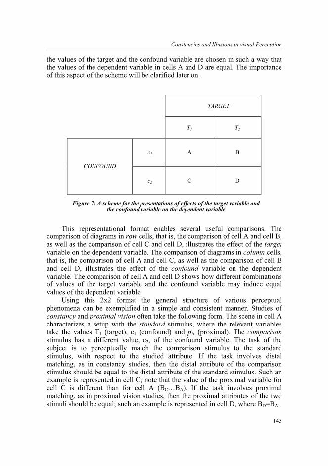
variable in all constancy and illusion examples will be illustrated according to a common scheme that consists of a 2x2 matrix of cells, schematically represented in Figure 7. Each of four cells (A, B, C, D) in the matrix contains a diagram depicting the effect of one value of the target variable T and one value of the confound variable c on the dependent variable. There are two values of the target variable (T1, T2), corresponding to columns, two values of the confound variable (c1 , c2), corresponding to rows, and four values of the dependent variable, corresponding to individual cells. A special characteristics of this scheme is that
Constancies and Illusions in visual Perception
143
the values of the target and the confound variable are chosen in such a way that the values of the dependent variable in cells A and D are equal. The importance of this aspect of the scheme will be clarified later on.
TARGET
T1
T2
c1 A B
CONFOUND c2 C D
Figure 7: A scheme for the presentations of effects of the target variable and
the confound variable on the dependent variable
This representational format enables several useful comparisons. The
comparison of diagrams in row cells, that is, the comparison of cell A and cell B, as well as the comparison of cell C and cell D, illustrates the effect of the target variable on the dependent variable. The comparison of diagrams in column cells, that is, the comparison of cell A and cell C, as well as the comparison of cell B and cell D, illustrates the effect of the confound variable on the dependent variable. The comparison of cell A and cell D shows how different combinations of values of the target variable and the confound variable may induce equal values of the dependent variable.
Using this 2x2 format the general structure of various perceptual phenomena can be exemplified in a simple and consistent manner. Studies of constancy and proximal vision often take the following form. The scene in cell A characterizes a setup with the standard stimulus, where the relevant variables take the values T1 (target), c1 (confound) and pA (proximal). The comparison stimulus has a different value, c2, of the confound variable. The task of the subject is to perceptually match the comparison stimulus to the standard stimulus, with respect to the studied attribute. If the task involves distal matching, as in constancy studies, then the distal attribute of the comparison stimulus should be equal to the distal attribute of the standard stimulus. Such an example is represented in cell C; note that the value of the proximal variable for cell C is different than for cell A (BC…BA). If the task involves proximal matching, as in proximal vision studies, then the proximal attributes of the two stimuli should be equal; such an example is represented in cell D, where BD=BA.

Dejan Todorović
144
Studies of illusions can be characterized in the following way. As in studies of constancy, a scene, such as in cell A, containing the standard stimulus, is contrasted with another scene, such as in cell C, containing the comparison stimulus, with the same value of the target variable but a different value, c2, of the confound variable. However, in illusion studies the manipulation of the confound variable does not affect the value of the proximal variable (thus BC=BA), but it does affect the value of the phenomenal variable. The contrast of the appearance of two scenes illustrates the effect of the illusion. The task of the subject is to manipulate or select the value of the target variable of the comparison stimulus, such that, as in the scene in cell D, the perceived value of the target variable matches the perceived value of the target variable in the scene in cell A. The discrepance in the values of target variables for scenes in cells A and D, which are perceptually matched, is a measure of the strength of the illusion. The contrast between the distal and the proximal variable, as well as the corresponding contrast between the perceived distal and perceived proximal variable, although crucial in the studies of constancies, is not essential in studies of illusions.

Constancies and Illusions in visual Perception
145
Basic aspects of all discussed constancies are presented in Figure 8. For
each type of constancy, this scheme includes a list of relevant variables (target, proximal, and confound), a depiction of their geometrical relation, and an analytic expression of this relation. The geometrical relations of the three variables are depicted schematically, and are meant to graphically convey the roles of the relevant variables in simple, basic cases. The corresponding equations mainly have the general form p = f(T, c), expressing the functional dependence of the proximal variable p on the target variable T and the confound variable c (such as the dependence of proximal size on distal size and distance).
Dejan Todorović
146
All subsequent discussions of constancies start with considerations of basic variables presented in the corresponding row of Figure 8, and are then elaborated using the 2x2 scheme introduced above. This is followed by the statement of the central problem, which involves the perceptual effects of the confound variable. Next, two types of appropriate phenomenal attributes are described, as well as the conditions of presentation which are used when these attributes are experimentally studied. After that, basic experimental results are briefly recounted. Finally, some relations between perceptual variables are considered. Namely, in some cases researchers have hypothesized that, corresponding to the functional relation p = f(T, c), holding between the non-phenomenal variables, an analogous relation of the form p' = f(T',c'), or some variant of it, holds in the phenomenal domain.
PART III: CONSTANCIES AND ILLUSIONS
The general considerations presented in Part II will now be concretely
illustrated with many examples of constancies and illusions. The exposition is divided in two parts, the first dealing with geometric attributes and the second with photometric attributes. Intrinsic geometric attributes (size and shape) and extrinsic geometric attributes (location and orientation) are discussed separately. Following that, both achromatic and chromatic aspects of photometric perception are discussed. Corresponding distal, proximal, and phenomenal attributes and their relations are analyzed for each kind of attribute (size, shape, location, orientation, and color). The sections concerning each attribute are divided into subsections on constancies and illusions. Each subsection contains one or more examples involving the 2x2 scheme introduced above.
A. Perception of extension - intrinsic geometric attributes Distal size and shape are intrinsic geometric attributes of distal objects. As
such, they are unaffected when these objects undergo changes of extrinsic attributes of location and orientation. Neither are they affected by the simultaneous presence of other objects in the scene. However, as will be discussed in this section, such circumstances may, in some conditions, affect the perception of size and shape.
1. Perception of size The general structure of size constancies and illusions will be presented in
this section. These discussions set the format for the subsequent discussions of all other constancies and illusions, and will therefore be formulated in more detail. Reviews of size constancy research are given by Baird (1970), Hochberg

Constancies and Illusions in visual Perception
147
(1971a), Rock (1975), Sedgwick (1986), and Gillam (1995). Reviews of size illusions can be found in Robinson (1972), Rock (1975), and Coren & Girgus (1978).
Depending on the domain, three types of size can be distinguished: distal, proximal, and phenomenal. Distal size is a relatively simple geometric attribute that can be numerically expressed with a single number. It comprises lengths of linear extents, areas of portions of 2-D surfaces, and volumes of portions of space. Distal size is also referred to as 'objective' or 'physical' or 'bodily' or 'linear size'. Proximal size refers to the sizes of projections of extended distal objects on the retina, expressed in angular terms. It is also called 'angular' or 'retinal' or 'projective' size. Perceived size refers to the conscious impression of external size. As it will be discussed below, it comes in two variants, one associated with distal size and the other with proximal size.
(a) Size constancy Studies of size constancy form a part of size perception research that is
concerned with perceptual effects of confound variables that affect the proximal size of distal objects. There are two such confound variables, distance and slant.
(i) Size constancy with respect to distance. Target, proximal, and confound variables. Several basic aspects of a setup often used in studies of size constancy are schematically presented in Figure 8, row 1. It contains a distal object, depicted as a vertical line, and an observer, represented by the retina. The target variable is the distal size S of the line. The corresponding proximal variable is the visual angle a that the projection of the line subtends on the retina; this variable is called 'proximal' or 'retinal' or 'angular' size. The confound variable is the distance d of the stimulus line, defined as the distance from the nodal point to the point where the stimulus line touches the visual axis. Note that in this setup the stimulus line is perpendicular to the visual axis.
The proximal variable, angular size α, depends not only on the target variable, distal size S, but also on the confound variable, distance d. The dependence of α on both S and d in this setup is expressed analytically by the formula α = atan (S/d). For example, a line of distal size S = 1 cm at the distance of d = 57 cm subtends a visual angle of α = 1o on the retina.
The 2x2 scheme. The relation between the three variables is further represented graphically in Figure 9, using the 2x2 scheme introduced in part II. The cells in the left column of the figure involve one value (S1) of the size S of the stimulus line, and the cells in the right column involve another, larger value (S2). Similarly, the cells in the top row of the figure involve one value (d1) of distance d of the stimulus line, whereas the cells in the bottom row involve another, larger value (d2). Cell A depicts a basic, initial situation. Cell B depicts a longer line at the same distance as in cell A. Cell C depicts a line of the same length as in cell A but at a larger distance. Finally, cell D depicts the longer line

Dejan Todorović
148
at the larger distance. The size and the distance are chosen in such a way that αD= αA, that is, the proximal size in cell D is the same as in cell A.
The comparison of cells A and B (and also of C and D) illustrates the dependence of proximal size on distal size: an increase of distal size causes an increase of proximal size (i.e., αB >αA, αD >αC) The comparison of cells A and C (and also of B and D) illustrates the dependence of proximal size on distance: an increase of distance causes a decrease of proximal size (i.e., αC<αA, αD<αB). Thus proximal size varies directly with distal size but inversely with distance. The comparison of cells A and D shows that different distal sizes may project into the same proximal size, a fact inverse to the fact that the same distal size may project into different proximal sizes. Both facts illustrate cases of distal-proximal discordance.
Perceptual effects of the confound variable. The foregoing discussion has
involved only the relations between the distal and the proximal domain, and was purely geometrical. The crucial issue in the present context, however, is the perception of size. The relations between the external domains and the phenomenal domain are probed in psychophysical experiments in which subjects are asked to match the size of a comparison stimulus to the size of the given
Constancies and Illusions in visual Perception
149
standard stimulus. The critical factor in such studies is the value of the confound variable, that is, the distance of the stimuli from the observer.
If the comparison stimulus is at the same distance as the standard stimulus, then the scene and the image are in concordance: two objects of equal (different) distal sizes also have equal (different) proximal sizes. If the two objects are also perceived as having equal (different) size, then all three domains are in concordance. However, this is not necessarily the case. As it is shown in the section on size illusions, if two lines are equally long and at the same distance, but if their contexts are different, or if they differ in location or orientation, the perceptual equality may not hold.
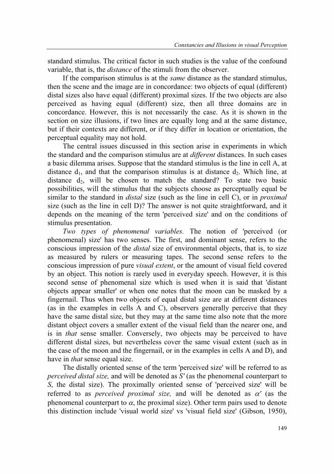
The central issues discussed in this section arise in experiments in which the standard and the comparison stimulus are at different distances. In such cases a basic dilemma arises. Suppose that the standard stimulus is the line in cell A, at distance d1, and that the comparison stimulus is at distance d2. Which line, at distance d2, will be chosen to match the standard? To state two basic possibilities, will the stimulus that the subjects choose as perceptually equal be similar to the standard in distal size (such as the line in cell C), or in proximal size (such as the line in cell D)? The answer is not quite straightforward, and it depends on the meaning of the term 'perceived size' and on the conditions of stimulus presentation.
Two types of phenomenal variables. The notion of 'perceived (or phenomenal) size' has two senses. The first, and dominant sense, refers to the conscious impression of the distal size of environmental objects, that is, to size as measured by rulers or measuring tapes. The second sense refers to the conscious impression of pure visual extent, or the amount of visual field covered by an object. This notion is rarely used in everyday speech. However, it is this second sense of phenomenal size which is used when it is said that 'distant objects appear smaller' or when one notes that the moon can be masked by a fingernail. Thus when two objects of equal distal size are at different distances (as in the examples in cells A and C), observers generally perceive that they have the same distal size, but they may at the same time also note that the more distant object covers a smaller extent of the visual field than the nearer one, and is in that sense smaller. Conversely, two objects may be perceived to have different distal sizes, but nevertheless cover the same visual extent (such as in the case of the moon and the fingernail, or in the examples in cells A and D), and have in that sense equal size.
The distally oriented sense of the term 'perceived size' will be referred to as perceived distal size, and will be denoted as S' (as the phenomenal counterpart to S, the distal size). The proximally oriented sense of 'perceived size' will be referred to as perceived proximal size, and will be denoted as α' (as the phenomenal counterpart to α, the proximal size). Other term pairs used to denote this distinction include 'visual world size' vs 'visual field size' (Gibson, 1950),
Dejan Todorović
150
and 'apparent absolute size' vs 'apparent angular size' (Joynson, 1949). Both senses of perceived size are externally oriented, that is, they are both phenomenal correlates of physically specifiable attributes, one distal and the other proximal. Although in everyday life the distal sense is almost exclusively used, the proximal sense can readily be noticed and attended to, once it is pointed out.
Note that our oculomotor systems are not guided by distal but by proximal size: when I look from one end of an object to the other, the amount of my eye rotation is guided, quite sensibly, by the proximal and not by the distal size of the object. Thus although I may note that objects in cells A and C have equal distal sizes, my eye excursions while inspecting them will be larger for the object in cell A than the object in cell C.
In size perception studies subjects are asked to match the comparison stimulus to the standard stimulus with respect to size. Since 'perceived size' does not have a unitary sense, it is clearly recommendable that the instructions to subjects explicitly indicate which attribute the experimenter has in mind. Distally focused instructions should stress that the matching comparison stimulus that 'looks the same size' as the standard stimulus should be objectively equal to the standard, e.g., when measured with a ruler. In contrast, proximally focused instructions, attempting to elicit judgements of perceived proximal size, are trickier to formulate. One possibility is to ask for a matching stimulus which would exactly mask the standard stimulus or could be visually superimposed upon it. Or, it can be required that the matching stimulus should be such that, if a photograph would be made of the standard and variable stimulus from the vantage point of the subject, their sizes, as measured on the photograph, would be equal (Gilinsky, 1955).
Sometimes instructions have been used which are unfocused, as when subjects are asked to produce the match according to the way the sizes of the stimuli 'look' or 'appear' to them, without more explicit explanations. The motivation for such instructions is the attempt to avoid possible cognitive biases that may be induced by distally or proximally focused instructions. However, these 'apparent' or 'look' instructions may be confusing. Given such instructions, the subjects are in fact left to decide what it is that the experimenter asks them to do. Different subjects understand such instructions in different ways, or may attend more to one than to the other aspect of perceived size (Joynson, 1949, 1958a,b; Joynson & Kirk, 1960). Furthermore, the same subject may change the response criterion during the experiment, or may try, within a single trial, to achieve a compromise of the two senses of perceived size. All of this may lead to average matches, which are intermediate between distal and proximal size, but are difficult to interpret.
Constancies and Illusions in visual Perception
151
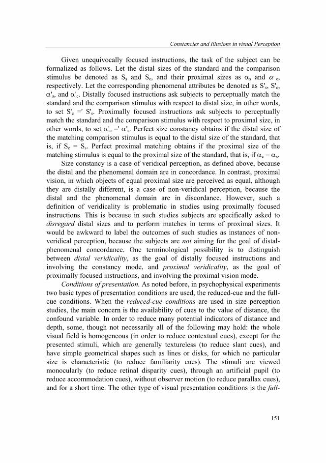
Given unequivocally focused instructions, the task of the subject can be formalized as follows. Let the distal sizes of the standard and the comparison stimulus be denoted as Ss and Sc, and their proximal sizes as αs and α c, respectively. Let the corresponding phenomenal attributes be denoted as S's, S'c, α's, and α'c. Distally focused instructions ask subjects to perceptually match the standard and the comparison stimulus with respect to distal size, in other words, to set S'c =' S's. Proximally focused instructions ask subjects to perceptually match the standard and the comparison stimulus with respect to proximal size, in other words, to set α'c =' α's. Perfect size constancy obtains if the distal size of the matching comparison stimulus is equal to the distal size of the standard, that is, if Sc = Ss. Perfect proximal matching obtains if the proximal size of the matching stimulus is equal to the proximal size of the standard, that is, if αc = αs.
Size constancy is a case of veridical perception, as defined above, because the distal and the phenomenal domain are in concordance. In contrast, proximal vision, in which objects of equal proximal size are perceived as equal, although they are distally different, is a case of non-veridical perception, because the distal and the phenomenal domain are in discordance. However, such a definition of veridicality is problematic in studies using proximally focused instructions. This is because in such studies subjects are specifically asked to disregard distal sizes and to perform matches in terms of proximal sizes. It would be awkward to label the outcomes of such studies as instances of non-veridical perception, because the subjects are not aiming for the goal of distal-phenomenal concordance. One terminological possibility is to distinguish between distal veridicality, as the goal of distally focused instructions and involving the constancy mode, and proximal veridicality, as the goal of proximally focused instructions, and involving the proximal vision mode.
Conditions of presentation. As noted before, in psychophysical experiments two basic types of presentation conditions are used, the reduced-cue and the full-cue conditions. When the reduced-cue conditions are used in size perception studies, the main concern is the availability of cues to the value of distance, the confound variable. In order to reduce many potential indicators of distance and depth, some, though not necessarily all of the following may hold: the whole visual field is homogeneous (in order to reduce contextual cues), except for the presented stimuli, which are generally textureless (to reduce slant cues), and have simple geometrical shapes such as lines or disks, for which no particular size is characteristic (to reduce familiarity cues). The stimuli are viewed monocularly (to reduce retinal disparity cues), through an artificial pupil (to reduce accommodation cues), without observer motion (to reduce parallax cues), and for a short time. The other type of visual presentation conditions is the full-

Dejan Todorović
152
cue condition, that is, a more or less natural viewing situation in which some, though not necessarily all standard distance cues are available.
Basic experimental results. The results of size perception studies depend on presentation conditions. Under completely reduced-cue conditions the comparison stimulus that the subjects match to the standard stimulus is generally such that its proximal size is fairly close to the proximal size of the standard, regardless of the distal sizes of the two stimuli (Lichten & Lurie, 1950; Hastorf & Way, 1952; Epstein, 1963; Rock & McDermott, 1964), even with distally focused instructions (Over, 1960). This is a natural outcome, because, when all cues to distance are eliminated, the proximal size remains as the main anchor that subjects can use for matching. Such results belong to the proximal vision mode, because the phenomenal attributes are in concordance with the proximal attributes, but both are in discordance with the distal attributes.
Under full-cue conditions, results depend on instructions. With distally focused instructions, the matching stimuli are generally such that their distal sizes are fairly close to the distal sizes of the standard stimuli, except that often (though not always) 'overconstancy' is obtained, that is, the matching sizes are consistently somewhat larger (distally) than the standard (Martius, 1889; Holway & Boring, 1941; Smith, 1953; Gilinsky, 1955; Jenkin, 1959; Carlson, 1960; Baird & Biersdorf, 1967). With proximally focused instructions the perceptually matching comparison sizes roughly correlate with the proximal sizes of the standard stimuli. However, the matching proximal sizes tend to be significantly larger than the standard proximal sizes. Furthermore, the results tend to be much more variable than results with distally focused instructions (Gilinsky, 1955; Epstein 1963; Carlson & Tassone, 1967; Leibowitz & Harvey, 1967).
If one believes that perception of distal size is generally veridical, then the departures from constancy must be explained. As noted above, matching values intermediate between distal and proximal sizes ('under-constancy') may be due to unfocused instructions. On the other hand, 'overconstancy' results may be due to conscious strategies of subjects who 'know that distant objects appear smaller' and therefore try to counter this tendency by choosing larger matching comparison stimuli (Carlson, 1960; Rock, 1975). However, rather than blaming unfocused instructions or misguided subject strategies, the possibility remains that distal size perception is not completely veridical, and that size constancy might fail to obtain due to genuine perceptual causes. Similar considerations apply to studies of proximal size. Judgements of visual angle may fail to agree with objective proximal size due to insufficiently clear instructions, special subject strategies, or perceptual causes.
Constancies and Illusions in visual Perception
153
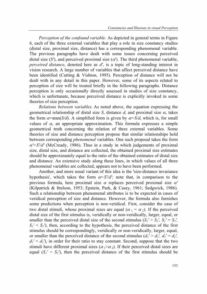
Perception of the confound variable. As depicted in general terms in Figure 6, each of the three external variables that play a role in size constancy studies (distal size, proximal size, distance) has a corresponding phenomenal variable. The previous paragraphs have dealt with some issues concerning perceived distal size (S'), and perceived proximal size (α'). The third phenomenal variable, perceived distance, denoted here as d', is a topic of long-standing interest in vision research. A large number of variables that affect perceived distance have been identified (Cutting & Vishton, 1995). Perception of distance will not be dealt with in any detail in this paper. However, some of its aspects related to perception of size will be treated briefly in the following paragraphs. Distance perception is only occasionally directly assessed in studies of size constancy, which is unfortunate, because perceived distance is explicitly invoked in some theories of size perception.
Relations between variables. As noted above, the equation expressing the geometrical relationship of distal size S, distance d, and proximal size α, takes the form α=atan(S/d). A simplified form is given by α=S/d, which is, for small values of α, an appropriate approximation. This formula expresses a simple geometrical truth concerning the relation of three external variables. Some theories of size and distance perception propose that similar relationships hold between corresponding phenomenal variables. One such proposal takes the form α'=S'/d' (McCready, 1986). Thus in a study in which judgements of proximal size, distal size, and distance are collected, the obtained proximal size estimates should be approximately equal to the ratio of the obtained estimates of distal size and distance. An extensive study along these lines, in which values of all three phenomenal variables are collected, appears not to have been performed.
Another, and more usual variant of this idea is the 'size-distance invariance hypothesis', which takes the form α=S'/d'; note that, in comparison to the previous formula, here proximal size α replaces perceived proximal size α' (Kilpatrick & Ittelson, 1953; Epstein, Park, & Casey, 1961; Sedgwick, 1986). Such a relationship between phenomenal attributes is to be expected in cases of veridical perception of size and distance. However, the formula also furnishes some predictions when perception is non-veridical. First, consider the case of two distal stimuli, whose proximal sizes are equal (α 1 = α 2). If the perceived distal size of the first stimulus is, veridically or non-veridically, larger, equal, or smaller than the perceived distal size of the second stimulus (S1' > S2', S1' = S2', S1' < S2'), then, according to the hypothesis, the perceived distance of the first stimulus should be correspondingly, veridically or non-veridically, larger, equal, or smaller than the perceived distance of the second stimulus (d1' > d2', d1' = d2', d1' < d2'), in order for their ratio to stay constant. Second, suppose that the two stimuli have different proximal sizes (α 1>α 2). If their perceived distal sizes are equal (S1' = S2'), then the perceived distance of the first stimulus should be

Dejan Todorović
154
smaller than the perceived distance of the second stimulus (d1' < d2'), whereas if their perceived distances are equal (d1' = d2'), then the perceived distal size of the first stimulus should be larger than the perceived distal size of the second one (S1' > S2'), regardless of veridicality.
Empirical support for the size-distance invariance hypothesis is equivocal (see Epstein, Park & Casey, 1961; Sedgwick, 1986). However, some data are clearly qualitatively consistent with this type of relationship between perceived distal size and perceived distance. An example is furnished by the well-known perceptual distortions in Ames' room (Ittelson, 1952). The rear wall of this room is objectively slanted in depth with respect to the perceiver, so that one of its back corners is objectively at a smaller distance than the other; therefore, if two objects of equal distal size are located in each corner, their proximal sizes are different, the one in the objectively nearer corner projecting a larger image (α 1 > α 2). However, the rear wall of Ames' room is, due to some, not generally agreed-upon cause, nonveridically perceived to be frontoparallel with respect to the observer, and thus the two back corners, and objects located near them, appear to be at equal distance (d1' = d2'). In accord with the above hypothesis, rather than veridically perceiving two objects of equal distal size located at different distances, observers perceive two objects of different distal size (S1' > S2') located at the same distance. A converse example concerns the percepts of the vertical edges of the back corners. The vertical edge of the nearer back corner in Ames' room is shorter, but both edges project equally long images (α 1 = α 2). However, as they are perceived to have equal distances (d1' = d2'), they are also perceived to have equal sizes (S1' = S2'). Within the present framework, these effects belongs to the mode of proximal vision, because objects of equal (different) proximal size also have equal (different) perceived sizes, although their distal sizes are different (equal).
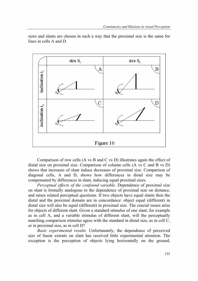
(ii) Size constancy with respect to slant. Target, proximal, and confound variable. Distance from the observer is not the only confound variable that, in addition to distal size, affects proximal size. Row 2 in Figure 8 depicts the dependence of proximal size on the slant of the distal object. Slant is defined here as the angle of inclination, i, of the object with respect to the perpendicular to the visual axis. The corresponding equation expresses the dependence of proximal size on distal size, distance, and slant. For example, a line of distal size S = 1 cm, slanted by angle i = 60o and at distance d = 57 cm, subtends an angle of size α = 0.5 o. In case of slant i = 0, the equation reduces to the previous case in which the stimulus line is perpendicular to the visual axis.
The 2x2 scheme. The dependence of proximal size on slant is also depicted with the help of the 2x2 scheme in Figure 10. The graphs in cells A and B are the same as in Figure 9, in which slant is zero. The cells C and D involve the same lines as in cells A and B, respectively, but with non-zero slant. The distal
Constancies and Illusions in visual Perception
155
sizes and slants are chosen in such a way that the proximal size is the same for lines in cells A and D.
Comparison of row cells (A vs B and C vs D) illustrates again the effect of
distal size on proximal size. Comparison of column cells (A vs C and B vs D) shows that increases of slant induce decreases of proximal size. Comparison of diagonal cells, A and D, shows how differences in distal size may be compensated by differences in slant, inducing equal proximal sizes.
Perceptual effects of the confound variable. Dependence of proximal size on slant is formally analogous to the dependence of proximal size on distance, and raises related perceptual questions. If two objects have equal slants then the distal and the proximal domain are in concordance: object equal (different) in distal size will also be equal (different) in proximal size. The crucial issues arise for objects of different slant. Given a standard stimulus of one slant, for example as in cell A, and a variable stimulus of different slant, will the perceptually matching comparison stimulus agree with the standard in distal size, as in cell C, or in proximal size, as in cell D?
Basic experimental results. Unfortunately, the dependence of perceived size of linear extents on slant has received little experimental attention. The exception is the perception of objects lying horizontally on the ground,

Dejan Todorović
156
stretching away from the observer, viewed at an angle from above, perceived under full-cue conditions, and studied with distally focused instructions: such extents appear as shorter than extents of equal length in vertical orientation (Wagner, 1985; Toye, 1986; Higashiyama & Ueyama, 1988; Levin & Haber, 1993; Norman, Todd, Perotti & Tittle, 1996). However, the manipulation of slant has received much more attention in the study of figures more complex than lines. This aspect will be dealt with in the section on shape perception.
(b) Size illusions In the discussions of size constancy the focus was on problems raised for
size perception by confound variables such as distance and slant, whose variations affect proximal size. I will now discuss a second set of problems involved in size perception, raised by a class of confound variables that do not affect proximal size but do affect perceived size. Size illusions involve phenomena in which objects of equal distal and proximal size nevertheless have different perceived sizes, or, conversely, cases in which objects of different distal and proximal size nevertheless have equal perceived sizes.
As noted in part II, the representational format for the description of size (and all other) illusions is similar to the one used for constancies. It involves the effect of a target and a confound variable on a dependent variable, demonstrated using a 2x2 scheme. The target variable is distal size. The dependent variable is not proximal size (as in size constancy studies) but perceived size. The values of distal size and the values of the confound variables are chosen such that the perceived sizes in cells A and D of the 2x2 scheme are approximately equal. Effects of three types of confound variables will be demonstrated.
In studies of size illusions, the variables 'distance' and 'slant', which are confound variables in studies of size constancy, are either held constant or their manipulation does not affect proximal size. Thus stimuli of equal (or different) distal size also have equal (or different) proximal size. In other words, the distal and the proximal domain are in concordance, and the distinction between distal and proximal size is not essential for the purpose of the discussion of the structure of results. Similarly, the distinction between perceived distal and perceived proximal size is generally not used in size illusion studies. Analogous considerations apply for other illusions.
(i) The dependence of perceived size on context. Many visual illusions can be described within a context vs. no-context framework. That is, the comparison is between stimuli presented in isolation and the same stimuli presented simultaneously with some other stimuli. Since the original stimulus is physically unchanged by the addition of context, it has identical distal size in both cases. A variant of this framework is the comparison of perceptual attributes of stimuli

Constancies and Illusions in visual Perception
157
presented in two different contexts. This is in fact the more general case, since no-context can be regarded as a special case of context.
An example of a size illusion presented in the 'context vs. no-context' framework is depicted Figure 11. Cells A and B contain two lines presented in isolation, with the second one objectively (distally and proximally) shorter. Cells C and D contain the same lines, but with the addition of several shorter lines ('fins'). Such stimuli are known as 'fins-out' versions of the Müller-Lyer figures. Distal size is the target variable, and the presence of context is the confound variable. Note that all stimuli have approximately the same distance and slant with respect to the observer.
Comparison of row cells (A vs B and C vs D) illustrates the trivial fact that
perceived size depends on distal size. Comparison of column cells (A vs C and B vs D) illustrates the interesting fact that perceived size depends on the presence of context.
In psychophysical matching studies of this effect, when the adjustment procedure is used subjects are asked to adjust the length of a comparison line without context until it looks the same size as a standard line in the fins-out context, or vice versa. Another possibility is to use the selection procedure and

Dejan Todorović
158
to present an array of lines of different lengths without context and to ask the subject to pick out the one which looks the same size as a particular standard line in the fins-out context, or vice versa. Whatever the procedure, the phenomenally matching line usually has a different distal size than the standard. The discrepancy of distal sizes is a measure of the strength of the illusion.
As it can be seen in the figure, lines without context look shorter than lines of equal length in the fins-out context. For example, the line in cell A looks shorter than the objectively equally long line in cell C. In contrast, the line in cell A looks approximately equal in length to the line in cell D, although the latter is objectively shorter.
An example of the 'different contexts' framework is presented in figure 12, featuring both 'fins-in' and 'fins-out' version of the Müller-Lyer figures. Cells A and B contain lines of different lengths, both with fins in, and cells C and D contain the same lines but with fins out. It can be seen that lines with fins in look shorter than the same lines with fins out. Note that lines in cell A and cell D look approximately equally long, although the latter is in fact objectively 25% shorter. This percentage is a measure of the strength of the illusion. Many figural variants and quantitative parameters of this illusion were studied (see reviews in Coren & Girgus, 1978, and Robinson, 1972).
The Müller-Lyer illusion is only one among many contextually
dependent size illusions. Some of them involve linear extents (Sander

Constancies and Illusions in visual Perception
159
illusion, Ponzo illusion, Opel-Kundt illusion) whereas other involve figure areas (Ebbinghaus illusion, Delboef illusion, Jastrow illusion). They can all be represented in the 2x2 format used above.
Note that in all examples the comparison of column cells (A vs C and B vs D), shows that lines of equal external (distal and proximal) size may have different perceived size, whereas the comparison of cells A and D shows that lines of different distal and proximal size may have equal perceived size. Thus in all these cases the distal and the proximal domain are in concordance, but both are discordant with the phenomenal domain, which is the characteristic of the illusion mode.
(ii) The dependence of perceived size on orientation. As it was shown in the section on size constancy, manipulation of slant of lines (the angle with respect to the visual axis) changes their proximal size. There is another component of line orientation, the tilt, whose variation preserves proximal size. Consider the simple case of a line belonging to the view-normal plane, defined here as any plane that is perpendicular to the visual axis. The slant of such a line is zero. If the line is rotated about the visual axis (as, for example, the hand of a clock rotates about the center), its spatial orientation will change. However, it will remain in the view-normal plane, its slant will stay zero, and its proximal size (the length of its projection on the retina) will stay constant. The aspect of orientation that does change with such a manipulation is defined here as the line's tilt. As it will be discussed in more detail in the section on perception of orientation, tilt can be defined by the angle that the line subtends with respect to some reference orientation, such as the vertical or the horizontal orientation. Note that when a line with non-zero slant is subjected to the same manipulation (rotation about the visual axis), its slant and proximal size will also remain unchanged. For such lines tilt can be defined as equal to the tilt of their projection upon the view-normal plane. However, such cases were rarely studied in experiments concerned with size illusions, and I will only consider zero slant lines in the following.
Although the manipulation of tilt does not change a line's proximal size, it may change its perceived size. The dependence of the phenomenal variable 'perceived size' on the target variable 'distal size' and the confound variable 'orientation' is illustrated in Figure 13. The lines in cells A and B are both in horizontal orientation, but the second one is slightly shorter. Corresponding lines of equal size are presented in cells C and D in vertical orientation.

Dejan Todorović
160
The effect of distal size on perceived size is again illustrated in the
comparison of row cells (A vs B and C vs D). The comparison of column cells (A vs C and B vs D), on the other hand, shows that orientation also affects perceived size, though to a small extent: the horizontal lines look slightly shorter than the corresponding vertical lines of equal objective size. Thus the line in cell A looks shorter than the line in cell C, although their distal sizes are equal, whereas it looks approximately equal in size to the line in cell D, although its distal size is slightly longer. The difference in objective size of perceptually equally long lines in cells A and D is a measure of the strength of the effect.
The presented effect is a variant of the 'vertical-horizontal' illusion. Note that when the head is tilted 90o the perceived length relations are reversed, and the objectively horizontal line looks longer than the objectively vertical line. Thus the relevant variable is not the exocentric, environment-relative orientation, but the orientation of the line on the subjects retina (see review in Robinson, 1972)

Constancies and Illusions in visual Perception
161
(iii) The dependence of perceived size on location. Perceived size depends
to some extent on the retinal locus that it is projected upon. This is illustrated in Figure 14. The effect is not demonstrated directly, as in previous two illusions, but indirectly, by depicting the situation in which it occurs, as in the constancy examples. Cell A depicts a situation in which the projection of an distal line is centered on the fovea; the inset in the lower right-hand corner depicts the corresponding retinal projection. Cell B depicts a distally longer line at the same distance, whose proximal length is also longer. Cell C depicts a situation in which the line from cell A is rotated about the vertical axis through the nodal point into a new position so that it projects onto the periphery of the retina. In cell D the same manipulation is performed on the line from cell B. Note that, in contrast to the examples in the section on size constancy, this manipulation preserves proximal size: the projections of lines in cells A and B have the same size as the projections of lines in cells C and D, respectively.
Experiments using similar manipulations have shown that extents projected at peripheral locations look shorter than extents of equal distal size, which are projected more centrally. Thus the line in cell A would look longer than the line in cell C. Conversely, the line in cell A would look approximately equally long as the line in cell D, although the latter is distally and proximally longer (Hillebrand, 1928; Schneider et al., 1978).

Dejan Todorović
162
2. Perception of shape Three kinds of shape will be considered, distal, proximal and
phenomenal. Distal shape is a relatively complex mathematical property. I will only consider the shapes of lines and contours of 2-D figures, because such shapes were predominantly used in studies of shape constancies and illusions. Proximal shape is the shape of projections of distal lines and contours upon the retina. I will disregard the fact that the retina is a curved surface and that the projections are thus also curved to a smaller or greater extent. Phenomenal shape comes in two variants, as perceived distal shape and perceived proximal shape.
Reviews of shape constancy are provided by Epstein & Park (1963) and Sedgwick (1986). Many shape illusions are presented by Coren & Girgus (1978) and Robinson (1972).
(a) Shape constancy Target, proximal, and confound variables. When an external object is
projected on the retina, its distal shape is projected into the proximal shape. However, the structure of the proximal shape is affected not only by the distal shape, as the target variable, but also by the slant of the object with respect to the visual axis, as the confound variable.
The 2x2 scheme. The dependence of proximal shape on distal shape and slant is presented in Figure 15. In cell A, a circular figure is viewed by an observer whose visual axis is perpendicular to the plane of the circle. The proximal shape, also a circle, is represented in the inset in the lower right-hand corner of cell A. In cell B another distal shape, a vertically elongated ellipse, is presented as the distal object; this is also the shape of the corresponding projection. In cell C the shape from cell A is slanted with respect to the visual axis. As a consequence, the corresponding proximal shape is a horizontally elongated ellipse. Finally, in cell D the second shape is also slanted, and its projected shape is circular, the same as the projected shape in cell A.
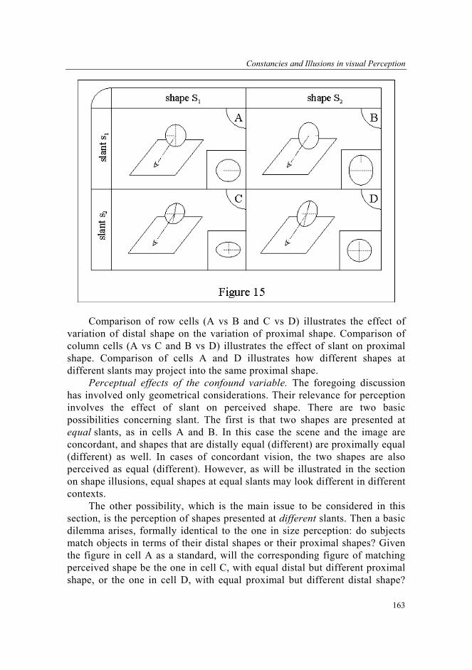
Constancies and Illusions in visual Perception
163
Comparison of row cells (A vs B and C vs D) illustrates the effect of
variation of distal shape on the variation of proximal shape. Comparison of column cells (A vs C and B vs D) illustrates the effect of slant on proximal shape. Comparison of cells A and D illustrates how different shapes at different slants may project into the same proximal shape.
Perceptual effects of the confound variable. The foregoing discussion has involved only geometrical considerations. Their relevance for perception involves the effect of slant on perceived shape. There are two basic possibilities concerning slant. The first is that two shapes are presented at equal slants, as in cells A and B. In this case the scene and the image are concordant, and shapes that are distally equal (different) are proximally equal (different) as well. In cases of concordant vision, the two shapes are also perceived as equal (different). However, as will be illustrated in the section on shape illusions, equal shapes at equal slants may look different in different contexts.
The other possibility, which is the main issue to be considered in this section, is the perception of shapes presented at different slants. Then a basic dilemma arises, formally identical to the one in size perception: do subjects match objects in terms of their distal shapes or their proximal shapes? Given the figure in cell A as a standard, will the corresponding figure of matching perceived shape be the one in cell C, with equal distal but different proximal shape, or the one in cell D, with equal proximal but different distal shape?

Dejan Todorović
164
The answer depends on the meaning of the term 'perceived shape' as well as on presentation conditions.
Two types of phenomenal variables. Similar to 'perceived size', the notion of 'perceived shape' has two senses, referred to here as perceived distal shape and perceived proximal shape. The first phenomenal attribute expresses the sense of 'shape' used in everyday life, and refers to the impression of an intrinsic geometric characteristic of objects that is independent of their position in space. In contrast, the second phenomenal attribute refers to the impression of the shape of the portion of the visual field covered by the object. This attribute changes with the change of object slant. Thus although subjects may declare that the disks in cells A and C have equal perceived distal shape, they may at the same time also note that the first disk covers a circular portion of the visual field whereas the second disk covers an elliptical portion of the visual field; thus the perceived proximal shapes of the two disks would be different. Conversely, disks in cells A and D would have different perceived distal shapes but similar perceived proximal shapes, because they cover equally shaped portions of the visual field. The conceptual distinction between two types of perceived space is also denoted by the contrast between the terms 'perceived objective shape' vs perceived 'projective shape' (see Sedgwick, 1986).
Note that it is not the distal shapes but the proximal shapes that guide oculomotor behavior. When I let my gaze glide along the perimeters of the disks in cell A and cell C, my eye motions will be approximately circular for the disk in cell A and approximately elliptical for the disk in cell C, even though I may perceive their distal shape to be identical.
As in the case of perceived size, the duality of the concept of perceived shape necessitates a corresponding duality of instructions to subjects in shape perception research. Distally focused instructions should clearly indicate that shapes perceived as equal should be objectively equal, for example, being exactly physically superimposable. In contrast, proximally focused instructions should stress the projective equality of the to-be-matched shapes. However, as in size perception research, authors of shape perception studies sometimes use 'apparent' or 'look' instructions that don't clearly identify the matching criterion. As Sedgwick (1986) remarks, the results of such studies, in which matching shapes tend to be intermediate between distal and proximal shapes, are 'not very informative', much for the same reasons as in size perception studies. Results of experiments by Joynson & Newson (1962) and Lichte & Borresen (1967) indicate that some subjects interpret such instructions as referring to distal shape, and others as referring to proximal shape.
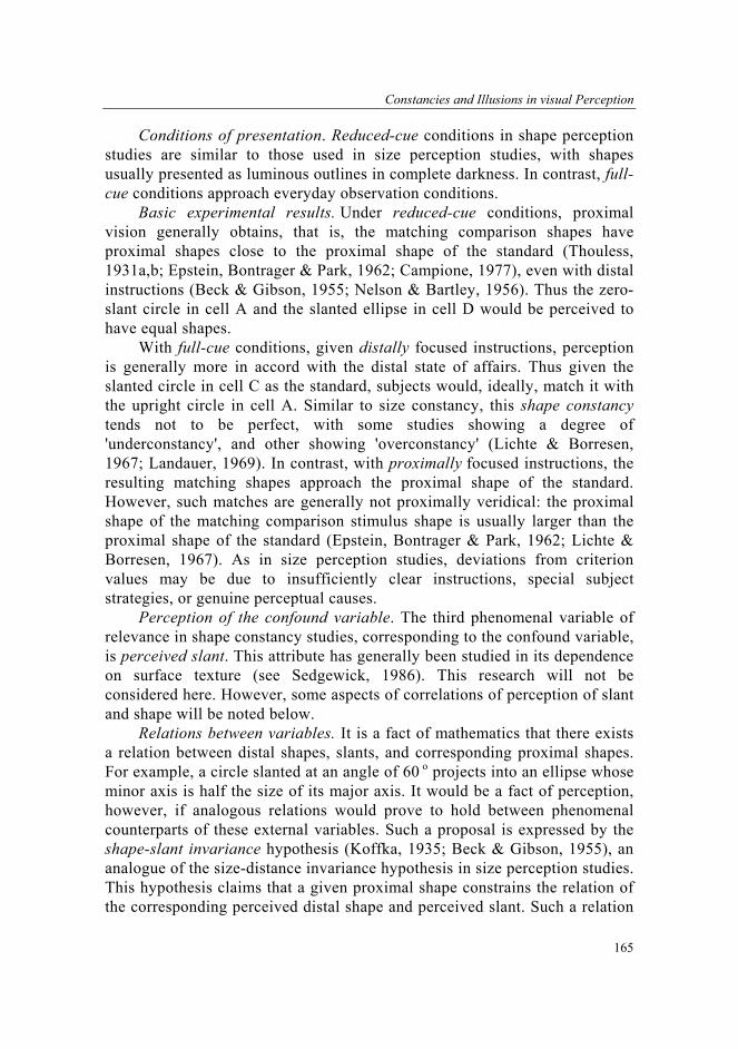
Constancies and Illusions in visual Perception
165
Conditions of presentation. Reduced-cue conditions in shape perception studies are similar to those used in size perception studies, with shapes usually presented as luminous outlines in complete darkness. In contrast, full-cue conditions approach everyday observation conditions.
Basic experimental results. Under reduced-cue conditions, proximal vision generally obtains, that is, the matching comparison shapes have proximal shapes close to the proximal shape of the standard (Thouless, 1931a,b; Epstein, Bontrager & Park, 1962; Campione, 1977), even with distal instructions (Beck & Gibson, 1955; Nelson & Bartley, 1956). Thus the zero-slant circle in cell A and the slanted ellipse in cell D would be perceived to have equal shapes.
With full-cue conditions, given distally focused instructions, perception is generally more in accord with the distal state of affairs. Thus given the slanted circle in cell C as the standard, subjects would, ideally, match it with the upright circle in cell A. Similar to size constancy, this shape constancy tends not to be perfect, with some studies showing a degree of 'underconstancy', and other showing 'overconstancy' (Lichte & Borresen, 1967; Landauer, 1969). In contrast, with proximally focused instructions, the resulting matching shapes approach the proximal shape of the standard. However, such matches are generally not proximally veridical: the proximal shape of the matching comparison stimulus shape is usually larger than the proximal shape of the standard (Epstein, Bontrager & Park, 1962; Lichte & Borresen, 1967). As in size perception studies, deviations from criterion values may be due to insufficiently clear instructions, special subject strategies, or genuine perceptual causes.
Perception of the confound variable. The third phenomenal variable of relevance in shape constancy studies, corresponding to the confound variable, is perceived slant. This attribute has generally been studied in its dependence on surface texture (see Sedgewick, 1986). This research will not be considered here. However, some aspects of correlations of perception of slant and shape will be noted below.
Relations between variables. It is a fact of mathematics that there exists a relation between distal shapes, slants, and corresponding proximal shapes. For example, a circle slanted at an angle of 60 o projects into an ellipse whose minor axis is half the size of its major axis. It would be a fact of perception, however, if analogous relations would prove to hold between phenomenal counterparts of these external variables. Such a proposal is expressed by the shape-slant invariance hypothesis (Koffka, 1935; Beck & Gibson, 1955), an analogue of the size-distance invariance hypothesis in size perception studies. This hypothesis claims that a given proximal shape constrains the relation of the corresponding perceived distal shape and perceived slant. Such a relation
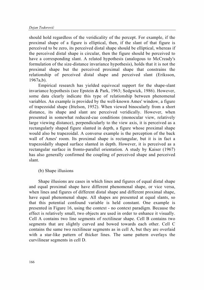
Dejan Todorović
166
should hold regardless of the veridicality of the percept. For example, if the proximal shape of a figure is elliptical, then, if the slant of that figure is perceived to be zero, its perceived distal shape should be elliptical, whereas if the perceived distal shape is circular, then the figure should be perceived to have a corresponding slant. A related hypothesis (analogous to McCready's formulation of the size-distance invariance hypothesis), holds that it is not the proximal shape but the perceived proximal shape that constrains the relationship of perceived distal shape and perceived slant (Eriksson, 1967a,b).
Empirical research has yielded equivocal support for the shape-slant invariance hypothesis (see Epstein & Park, 1963; Sedgwick, 1986). However, some data clearly indicate this type of relationship between phenomenal variables. An example is provided by the well-known Ames' window, a figure of trapezoidal shape (Ittelson, 1952). When viewed binocularly from a short distance, its shape and slant are perceived veridically. However, when presented in somewhat reduced-cue conditions (monocular view, relatively large viewing distance), perpendicularly to the view axis, it is perceived as a rectangularly shaped figure slanted in depth, a figure whose proximal shape would also be trapezoidal. A converse example is the perception of the back wall of Ames' room. Its proximal shape is rectangular, but it is in fact a trapezoidally shaped surface slanted in depth. However, it is perceived as a rectangular surface in fronto-parallel orientation. A study by Kaiser (1967) has also generally confirmed the coupling of perceived shape and perceived slant.
(b) Shape illusions Shape illusions are cases in which lines and figures of equal distal shape
and equal proximal shape have different phenomenal shape, or vice versa, when lines and figures of different distal shape and different proximal shape, have equal phenomenal shape. All shapes are presented at equal slants, so that this potential confound variable is held constant. One example is presented in Figure 16, using the context - no context paradigm. Because the effect is relatively small, two objects are used in order to enhance it visually. Cell A contains two line segments of rectilinear shape. Cell B contains two segments that are slightly curved and bowed towards each other. Cell C contains the same two rectilinear segments as in cell A, but they are overlaid with a star-like pattern of thicker lines. The same pattern overlays the curvilinear segments in cell D.

Constancies and Illusions in visual Perception
167
Note that the two segments in cell C, although objectively rectilinear,
appear somewhat curved and bowed away from each other. This effect is known as the 'Hering illusion'. In contrast, the two curvilinear segments in cell D appear approximately rectilinear, or at least more rectilinear than the segments in cell C. In cell D the effect of objective curvilinearity is opposed by the inversely directed effect of induced curvilinearity. Thus the figures of different external (distal and proximal) shape in cells A and D have similar perceived shape, whereas the figures of equal external shape in cells A and C have different perceived shape. A measure of the induced effect can be provided by the extent of objective curvilinearity that is needed to make the curves appear rectilinear. Related shape illusions were reported by Wundt (1898), Ehrenstein (1925), and Orbison (1939).
B. Perception of position - extrinsic geometric attributes As discussed in the introduction, the extrinsic geometric attributes are
location, decomposable into direction and distance, and orientation, decomposable into slant and tilt. There is an important difference between intrinsic and extrinsic geometric attributes. Size and shape, the intrinsic attributes, are independent from particular reference frames, in the sense that they can be defined independently from reference frames and that they remain the same in different reference frames. Locations and orientations of

Dejan Todorović
168
objects are reference frame dependent, because they must be defined with respect to some reference frame, and the same object may have different values of these attributes in different reference frames. The reference frames may appear in the form of reference points, lines, planes, other objects, or complete 3-D co-ordinate systems.
Reviews of location and orientation constancies and illusions can be found in Rock (1975), Shebilske (1977), Howard (1986), and Matin (1986).
1. Perception of location Three kinds of location can be distinguished, distal, proximal, and
phenomenal. These three kinds will be described in more detail in the following. Furthermore, different types of reference frames will be discussed. As noted before, reference frames for locations can be egocentric (perceiver-relative), or exocentric (environment-relative). Egocentric reference frames are based on some aspect of the body of the perceiver, whereas exocentric reference frames involve some aspect of the environment. In both cases there are several possible choices for reference frames. Some of these choices will be presented in the following.
Distal locations. One variant of an egocentric reference frame for distal locations can be constructed in the following way. Consider the mid-frontal plane of the head: this is the plane that divides the head into a front and back half; any plane parallel to that plane is a fronto-parallel plane. Furthermore, consider a line that is perpendicular to that plane. Such a line can be used to define the straight-ahead direction as a reference direction. There are several spatial positions that such a line may assume. For example, the line may be defined to pass through a point midway between the two eyes, or through the tip of the nose. The position that will be assumed in the following is for the line to pass through one of the eyes, because I will only treat monocular perception. More precisely, the reference line will be assumed to pass through the center of eye rotation: this is the imaginary point about which the eye is rotated in its socket. This point does not coincide with the nodal point of the eye; however, the difference between the two points is negligible for the purpose of the present discussion, and will disregarded.
All points which lie on the reference line in front of the subject, lie in the egocentric straight ahead direction. The egocentric directions of all other external points are defined by the lines connecting these points and the nodal point of the eye of the observer. These directions in 3-D can be defined with two angles, but I will not elaborate the appropriate geometrical constructions here; this is because in the examples I will, for simplicity, only use 2-D cross-sections

Constancies and Illusions in visual Perception
169
through 3-D space, and in such cases only one angle suffices to define the direction of any point, as will be shown below.
Note that the straight ahead direction and all other egocentric directions, as defined here, do not depend on eye motions: when the head is motionless, its mid-frontal plane and the reference line perpendicular to it remain in the same position, regardless of how the eyes may move with respect to the head.
One important aspect of the geometrical analysis is the orientation of the head with respect to gravity. When the head is vertical, that is, when its long axis is aligned with the direction of gravity, then the straight ahead direction is horizontal, that is, perpendicular to gravity. When the orientation of the head is not aligned with gravity, there are two possibilities. One possibility is that the head is rotated about some axis parallel to the straight ahead line. Such a possibility arises when the head is tilted toward one of the shoulders. In this case the straight ahead line is still horizontal. This possibility will be discussed in the section dealing with perception of orientation. In all the remaining cases the mid-frontal plane and the reference line change their spatial orientation, and thus the direction of straight ahead, as defined above, changes as well. Such cases will not be discussed here.
Let us return to the case when the head is vertical, which will be assumed further on. A geographically vertical plane through the horizontal straight ahead line divides the visual field of the subject into a right half and a left half. A geographically horizontal plane through the straight ahead line divides the visual field into a top half and a bottom half. Note that 'straight ahead' is sometimes defined as comprising all points of the vertical plane lying in front of the subject. Defined in that way, 'straight ahead' does not name a single direction but a family of directions. An analogous concept, 'eye level', denotes a family of directions of points lying in the horizontal plane described above. The vertical plane, the horizontal plane, and a fronto-parallel plane through the nodal point define a Cartesian co-ordinate system centered in the nodal point.
Note that other types of egocentric reference frames can also be defined. For example, a reference frame can be associated with the median or mid-sagittal plane of the body, a plane that divides the body into a right half and left half. This reference frame stays constant when only the head turns or tilts, but the rest of the body does not move.
The preceding discussion has dealt with examples of egocentric reference frames for distal locations. An example of an exocentric reference frame is the meeting place of any three walls in a room. Any location in the room can be defined with respect to a co-ordinate system with three walls as co-ordinate planes. Note that when an observer moves about in the room, the locations of points in the room with respect to the egocentric reference frames discussed above generally change. For example, what is located straight ahead of me at

Dejan Todorović
170
one instant may be located toward my left at the next instant, etc. However, the locations with respect to the exocentric reference frame remain, of course, the same.
Proximal locations. The second kind of location relevant for vision is proximal location, which is the location of a projected point on the retina. A reference frame associated with the retina can be defined in the following way. First, suppose that the head is vertical. Second, suppose that the eyes are in the, so called, primary position: this is the position in which the visual axis (the direction of gaze) is aligned with the straight ahead direction. In other words, the observer looks straight ahead. Then, the geographically vertical plane through the straight ahead line (or, equivalently, through the visual axis) defines a meridian on the retina that divides it into a left half and a right half, and the geographically horizontal plane defines a meridian that divides the retina into a top half and a bottom half. The two meridians, intersecting in the fovea, define a curvilinear co-ordinate system on the retina. They are sometimes referred to as the 'horizontal' and the 'vertical' meridian. However, these names are appropriate only when the eye is in the primary position; in other cases these meridians generally cease to lie in the vertical or horizontal plane. Taking into account the elliptical shape of the visual field, I will refer to the 'horizontal' meridian as the 'major-axis' meridian, and to the 'vertical' meridian as the 'minor-axis' meridian. The location of any point on the retina can be specified by its distances from the two meridians, measured in angular terms; another possibility is to specify location by the distance from the fovea and the angle that the line connecting the point and the fovea subtends with one of the meridians. In 1-D cross-sections through the retina, such as in Figure 3, which will be used in the following, only a single signed number suffices to specify the location of a retinal point, and that is the angular distance of the point from the fovea.
Phenomenal locations. The third relevant kind of location is phenomenal or perceived location, which refers to the conscious impression of locations of points. Perceived distal and perceived proximal location will be distinguished.
Perception of distance will not be considered here, and only the directional aspect of perceived location will be analyzed. Furthermore, only egocentric location will be discussed, since the perception of purely exocentrically defined location has attracted little interest in the context of studies of constancies.
(a) Direction constancy Target, proximal, and confound variable. The relations of three relevant
variables are represented in row 3 in Figure 8. The graphical sketch depicts a 2-D cross-section, as in Figure 3. The situation involves a distal object, depicted with an 'x', a retina, and several relevant directions. It is assumed

Constancies and Illusions in visual Perception
171
that the head is vertical, and thus that the straight ahead direction is horizontal, but that the eyes are not in the primary position. The target variable is egocentric object direction, indicated by the thick arrowed line. It is specified by the angle, D, that the line subtends with the reference, straight-ahead line, which is depicted by the dotted line in the figure. The corresponding proximal variable is the proximal location of the object, specified by the angular distance, α, of the projection point from the fovea (depicted by a small gray disk). The angle α depends not only on object direction but also on a confound variable, the gaze direction, indicated by a thin full line, extending perpendicularly from the fovea. Gaze direction is specified by the angle, g, that this line subtends with the straight-ahead line. Given a fixed distal object and fixed head position, when the gaze direction changes, the location of the projection of the external point changes as well. The relation between the three angular variables is given by the simple equation α = D - g. For example, if a distal object is located D = 30o away from straight ahead, and the gaze deviates g = 20o from straight ahead in the same direction, then the projection of the object is located at α = 10o from the fovea.
The 2x2 scheme. The effect of the distal and the confound variable on the proximal variable is further elaborated in Figure 17. Cell A depicts the simple situation in which all three directions (the direction of the object, the direction of the gaze, and the reference straight ahead direction) coincide, and all three angles are zero; the lines are drawn as slightly offset vertically. The object is located at the straight-ahead line, and the perceiver looks straight ahead, so that the object projects onto the fovea. The inset in the bottom right corner of cell A depicts the mutual spatial relation, on the retina, of the fovea and the retinal projection of the object; in this case, the two loci coincide. In cell B the object is located higher, but gaze direction is still straight ahead, so that, as shown in the inset, the object projects below the fovea. In cell C, the object direction is straight ahead, as in cell A, but the gaze is turned upwards, so that the object is projected above the fovea. In cell D, the gaze direction is equal to the object direction, and both deviate from straight ahead; the object projects into the fovea, as in cell A.

Dejan Todorović
172
Comparison of row cells illustrates how the proximal location of the
object depends on the target variable, the egocentric direction. Comparison of column cells shows how proximal location depends on gaze direction, the confound variable. Comparison of cells A and D shows how objects of different distal directions may have equal proximal locations, a fact inverse to the fact that objects of equal distal direction may have different proximal locations.
Perceptual effects of the confound variable. The previous discussion concerning the effect of gaze direction was purely geometrical. The crucial perceptual question, however, is how gaze direction affects perceived direction. There are two basic possibilities. The first possibility is that the perceiver looks straight ahead, that is, that the gaze direction coincides with the straight ahead direction, as in cells A and B. Then the egocentric direction of any object with respect to straight ahead is the same as with respect to the gaze direction. Furthermore, the distal egocentric direction of an object is in accord with the proximal location of its projection, in the sense that the direction with respect to straight ahead agrees with the location with respect to the fovea. In this case the projected location of an object specifies its egocentric direction and vice versa.
The second possibility is that gaze direction deviates from straight ahead. In this case a basic dilemma arises: are the perceived directions in accord with distal directions or with proximal locations? Again, the answer depends on the meaning of 'perceived direction'.

Constancies and Illusions in visual Perception
173
Two types of phenomenal variables. Two meanings of 'perceived (or phenomenal) egocentric direction' can be defined. The first meaning, which corresponds to the target variable, egocentric object direction D, will be referred to as 'perceived distal egocentric direction', and denoted as D'. This concept involves the conscious impression of the direction of external objects with respect to the head and the straight ahead direction. This meaning is exemplified in phrases such as 'object A lies directly straight ahead of me, object L is off to my left, and object R is off to my right'. Note that perceived distal egocentric direction, as defined here, does not depend on the direction of the gaze, provided that the head is fixed. However, it does depend on the position of the head. In the above example, if the head is turned toward object L, then that object comes to lie straight ahead, and object A comes to lie toward right.
The second sense of 'perceived egocentric direction' corresponds to the proximal variable α, the location of the projection of the external object on the retina. This notion will be referred to here as 'perceived proximal egocentric direction' and denoted as α '. Rock (1975) expresses the second sense of perceived egocentric direction by the terms 'perceived location in the visual field' and 'field location'. This notion refers to the conscious impression of the direction of an object within the momentary field of view and with respect to the current gaze direction. For example, when I look at object A from the previous example, its proximal location is at my fovea, and its perceived proximal direction is in my current gaze direction at the center of my current view. The proximal locations of other objects, such as L or R, are away from the fovea, and the corresponding perceived proximal directions are toward the periphery of my current field of view and away from my current gaze direction. When I switch my gaze from A to L then, provided that my head remains fixed, the perceived distal egocentric directions of these objects do not change: object A remains straight ahead and object L remains off to my left. However, the perceived proximal egocentric directions of these objects do change: object L is now at the center of my view, whereas object A lies toward the periphery.
Note that it is not distal locations but proximal locations that guide oculomotor behavior. In the preceding example, the distal egocentric direction of object A remains straight ahead regardless of eye motions. However, in order to move my gaze to the direction of point A, if my gaze is currently directed at point L, I must move the gaze toward the proximal direction of object A, that is, toward right, whereas if my gaze is currently directed at point R, I have to move it toward left.
Conditions of presentation and basic experimental results. Only perceived distal direction will be discussed here because, although perceived proximal location is occasionally discussed as a valid, though intuitively
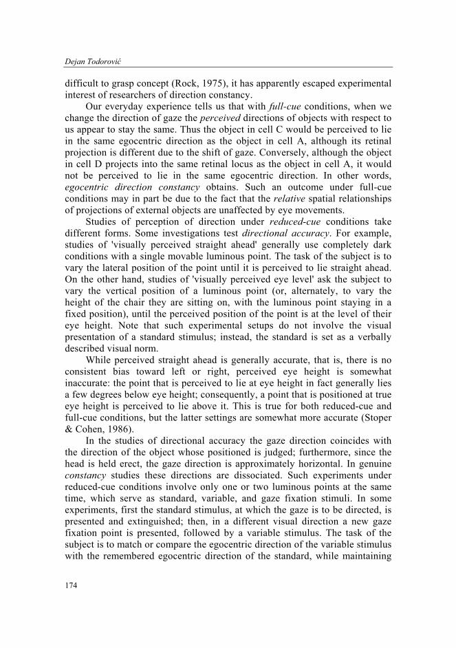
Dejan Todorović
174
difficult to grasp concept (Rock, 1975), it has apparently escaped experimental interest of researchers of direction constancy.
Our everyday experience tells us that with full-cue conditions, when we change the direction of gaze the perceived directions of objects with respect to us appear to stay the same. Thus the object in cell C would be perceived to lie in the same egocentric direction as the object in cell A, although its retinal projection is different due to the shift of gaze. Conversely, although the object in cell D projects into the same retinal locus as the object in cell A, it would not be perceived to lie in the same egocentric direction. In other words, egocentric direction constancy obtains. Such an outcome under full-cue conditions may in part be due to the fact that the relative spatial relationships of projections of external objects are unaffected by eye movements.
Studies of perception of direction under reduced-cue conditions take different forms. Some investigations test directional accuracy. For example, studies of 'visually perceived straight ahead' generally use completely dark conditions with a single movable luminous point. The task of the subject is to vary the lateral position of the point until it is perceived to lie straight ahead. On the other hand, studies of 'visually perceived eye level' ask the subject to vary the vertical position of a luminous point (or, alternately, to vary the height of the chair they are sitting on, with the luminous point staying in a fixed position), until the perceived position of the point is at the level of their eye height. Note that such experimental setups do not involve the visual presentation of a standard stimulus; instead, the standard is set as a verbally described visual norm.
While perceived straight ahead is generally accurate, that is, there is no consistent bias toward left or right, perceived eye height is somewhat inaccurate: the point that is perceived to lie at eye height in fact generally lies a few degrees below eye height; consequently, a point that is positioned at true eye height is perceived to lie above it. This is true for both reduced-cue and full-cue conditions, but the latter settings are somewhat more accurate (Stoper & Cohen, 1986).
In the studies of directional accuracy the gaze direction coincides with the direction of the object whose positioned is judged; furthermore, since the head is held erect, the gaze direction is approximately horizontal. In genuine constancy studies these directions are dissociated. Such experiments under reduced-cue conditions involve only one or two luminous points at the same time, which serve as standard, variable, and gaze fixation stimuli. In some experiments, first the standard stimulus, at which the gaze is to be directed, is presented and extinguished; then, in a different visual direction a new gaze fixation point is presented, followed by a variable stimulus. The task of the subject is to match or compare the egocentric direction of the variable stimulus with the remembered egocentric direction of the standard, while maintaining

Constancies and Illusions in visual Perception
175
the gaze at the new fixation point. In other experiments, the direction of the standard is described verbally but is not presented visually: with the gaze directed on a laterally displaced fixation point, the subject is told to set the variable stimulus such that it lies 'straight ahead'. The first type of experiment uses the 'matching-to-standard' procedure, whereas the second is an example of 'matching-to-norm' procedures.
Some studies find that, on average, egocentric direction constancy under reduced-cue conditions is relatively exact (Matin, 1986). Others find some underconstancy: the perceived straight ahead is somewhat displaced from the objective straight ahead towards the direction of the fixation point. For example, if the gaze is fixed at a point that lies 30o to the right of the straight ahead direction, then the variable stimulus that the subjects set as being located straight ahead is in fact located a few degrees towards right; this means that an object that is objectively straight ahead is perceived to be somewhat to the left of straight ahead (Hill, 1972; Morgan, 1978).
Perception of the confound variable. The foregoing sections have involved the phenomenal counterparts of egocentric distal direction (the target variable) and proximal location (the proximal variable). The third ingredient in direction constancy studies, objective gaze direction, g, which refers to the actual posture of the eye, also has a phenomenal counterpart, which will be called here 'perceived gaze direction', and denoted as g'. This notion refers to the felt position of the eye. Traditionally, discussions concerning gaze direction have mainly involved the problem of the organismic source of the information about gaze direction. It is generally believed that this information mainly stems from 'outflow', that is, the neural command to move the eyes, although 'inflow', the feedback information from eye muscles, may also play a role (Matin, 1986).
Relations between variables. As noted before, the relation between the non-phenomenal variables takes the form α = D - g. Based on this relation, the cancellation theory of direction constancy (see Matin, 1986), holds that constant perceived direction of objects (D' ), in the presence of eye movements, derives from the comparison and cancellation of neural representations of retinal displacement information (α) and eye position information (g).
Such a relation may also be the basis of some departures from direction constancy. For example, if, for a given retinal location of a stimulus, the information about eye position is inaccurate, then perceived direction should also be inaccurate. This idea is consistent with some data concerning after-effects of prolonged holding of the eyes in an eccentric position: when the eyes are relaxed again, the perceived straight ahead deviates for some time from the objective straight ahead toward the direction in which the eyes were held previously. This effect can be explained by the assumption that in this

Dejan Todorović
176
situation the eye muscles, for a while, reflexively tend to return (to some extent) to their previous posture, but that this tendency is not registered properly in the rest of the visual system. Thus the eyes may actually be turned somewhat to the side, say toward right, but with the observer feeling that they are in the primary position, that is, oriented straight ahead. Then a point whose image falls onto the fovea, which is in fact located toward right, will be perceived to lie straight ahead (Paap & Ebenholtz, 1976).
(b) Direction illusions Illusions of perceived direction arise when objects of equal egocentric
directions and equal proximal location have different perceived directions, or vice versa. Such an example is described in Figure 18. It involves reduced-cue conditions in which only a luminous point and a rectangular frame are visible. The example on the printed page is only an illustration, since it does not satisfy these conditions and thus the relevant effect is not actually detectable. Cell A depicts a display which contains a luminous point located at the straight-ahead line, surrounded by a rectangular frame whose center coincides with the point. The two dotted lines depict the geographic horizontal and vertical bisectors of the visual field, dividing it into a top and bottom half, and a left and right half. In cell B the point is dislocated to the right, and thus does not lie straight ahead. In cell C the point lies straight ahead, but the position of the rectangle is shifted to the right. In cell D both the point and the rectangle are shifted, but not to the same amount.
The direction illusion concerns the displays in which the position of the rectangle is eccentric. In such a case, if the point is located at the straight ahead line (as in cell C), it does not look straight ahead: instead it looks displaced to the left of perceived straight ahead. This is an instance of the Roelofs effect (Roelofs, 1935; Werner, Wapner, & Bruell, 1953; Bruell & Albee, 1955; Bridgeman, 1993). Consequently, the point that is perceived to lie straight ahead is a point whose egocentric direction is shifted to the right of objective straight ahead (as in cell D). Thus the perceived direction of straight ahead is shifted in the same direction in which the rectangle is shifted, though not to the same amount. The amount of shift is a measure of the strength of the effect.
Related illusions arise when subjects look into a box that is slanted upwards or downwards, or are placed, with head erect, into a similarly slanted room. In such cases the direction of visually perceived eye level is shifted vertically towards the direction of the slant of the box or the room (Li & Matin, 1995; Cohen, Ebenholtz & Linder, 1995; Welch & Post, 1996).
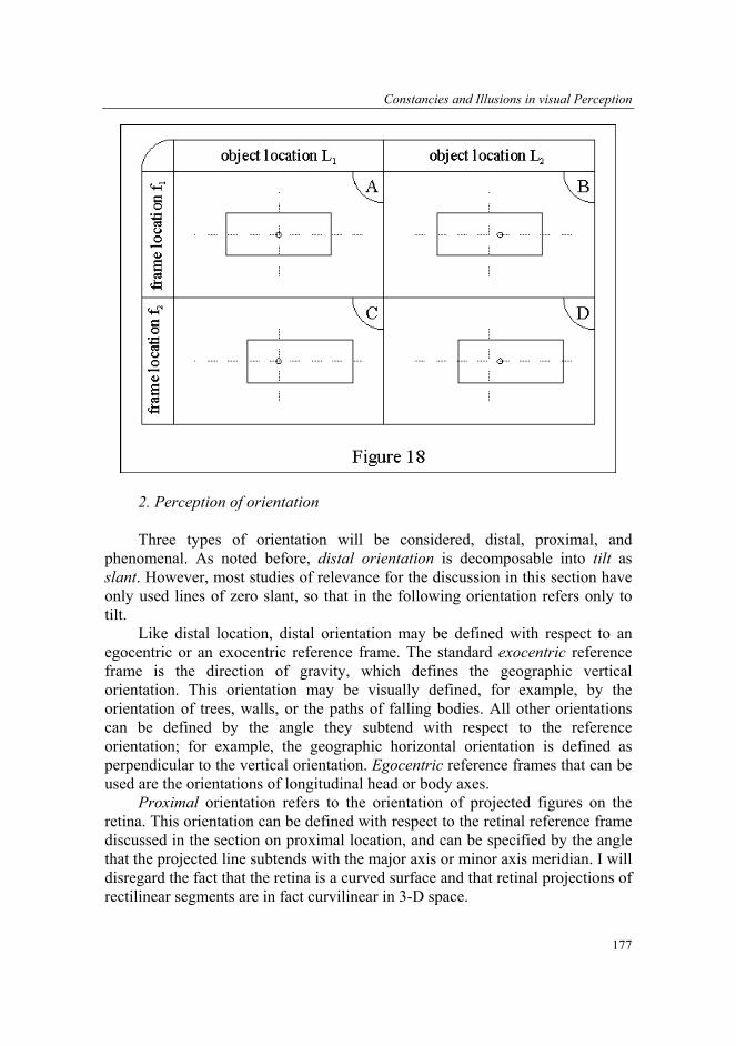
Constancies and Illusions in visual Perception
177
2. Perception of orientation Three types of orientation will be considered, distal, proximal, and
phenomenal. As noted before, distal orientation is decomposable into tilt as slant. However, most studies of relevance for the discussion in this section have only used lines of zero slant, so that in the following orientation refers only to tilt.
Like distal location, distal orientation may be defined with respect to an egocentric or an exocentric reference frame. The standard exocentric reference frame is the direction of gravity, which defines the geographic vertical orientation. This orientation may be visually defined, for example, by the orientation of trees, walls, or the paths of falling bodies. All other orientations can be defined by the angle they subtend with respect to the reference orientation; for example, the geographic horizontal orientation is defined as perpendicular to the vertical orientation. Egocentric reference frames that can be used are the orientations of longitudinal head or body axes.
Proximal orientation refers to the orientation of projected figures on the retina. This orientation can be defined with respect to the retinal reference frame discussed in the section on proximal location, and can be specified by the angle that the projected line subtends with the major axis or minor axis meridian. I will disregard the fact that the retina is a curved surface and that retinal projections of rectilinear segments are in fact curvilinear in 3-D space.

Dejan Todorović
178
Phenomenal orientation refers to the conscious impression of orientation. Perceived distal and perceived proximal variants of phenomenal orientation may be distinguished. Only perceived exocentric orientation will be discussed here, because few studies have dealt with pure egocentric orientation (but see Rock, 1975; Goodenough, Nowak, Oltman, Cox, & Sigman, 1982). In the following analyses, it will be assumed that the eyes are in the primary position.
(a) Orientation constancy Target, proximal, and confound variable. Three basic variables relevant for
perception of orientation in the sense of tilt, with respect to the exocentric gravitational reference frame, are listed in row 4 of Figure 8. The accompanying figure depicts the retinal surface as an ellipse. A thick line is depicted as a projection of a distal line on the retina. The reference orientation is the geographic horizontal, depicted as a dotted line. The target variable is distal orientation, defined here by the angle, O, that the distal line subtends with the geographic horizontal; this angle is the same as the angle that the projected line subtends with the geographic horizontal, as depicted in the figure. The proximal variable is proximal or retinal orientation, defined here by the angle, α, that the projection of the line subtends with the major axis retinal meridian, depicted as a full line. The retinal orientation α depends not only on object orientation O, but also on a confound variable, eye orientation, defined here by the angle, e, subtended by the major axis meridian and the geographic horizontal. The orientation of the eye deviates from the geographic horizontal when the head or the whole body is tilted. However, the eye tilt tends to be smaller than the corresponding head or body tilt, because of the effect of cyclotorsion, that is, a reflex counter rolling of the eyes in the direction opposite to tilt. As in the case of direction, the relation between the three relevant variables is very simple, and is given by α = O - e. For example, if a distal line is tilted by O = 30o with respect to the geographic horizontal, and the eye is tilted by e = 20o with respect to the same reference orientation, then the projected line is tilted by α = 10o with respect to the major-axis retinal meridian.
The 2x2 scheme. The effect of distal orientation and eye orientation on proximal orientation is elaborated in Figure 19, in a manner similar to the analysis of direction. Cell A depicts a case in which the orientation of the distal stimulus line, the retinal orientation of its projection, and the orientation of the eye all coincide with the geographic horizontal (the lines are drawn as vertically offset); thus all three angular variables are zero. In cell B the eye has the same orientation but the object is tilted with respect to geographic horizontal, and thus the projected line is tilted with respect to the retinal major axis meridian. In contrast, in cell C it is the eye which is tilted whereas the stimulus line is horizontal; consequently, the projected line is tilted with respect to the retinal

Constancies and Illusions in visual Perception
179
major axis meridian, but in the opposite direction than in cell B. In cell D both the stimulus object and the eye are tilted by the same amount in the same direction, so that the projected line is parallel to the retinal major axis meridian, as in cell A.
Comparison of row cells illustrates the effect of object orientation on proximal orientation. Comparison of column cells illustrates the effect of eye orientation on proximal orientation. Comparison of cells A and D shows how different combinations of object orientation and eye orientation can result in equal proximal orientations. Thus objects of equal distal orientation may have different proximal orientations, and vice versa.
Perceptual effects of the confound variable. The previous considerations were purely geometrical. The crucial perceptual issue concerns perceived object orientation. There are two basic possibilities. One possibility obtains when the head is erect. Then the orientations of the major-axis and minor-axis retinal meridians coincide with the geographic horizontal and vertical. In this case distal orientation agrees with proximal orientation, in the sense that the distal tilt of a line, with respect to the exocentric reference frame, is the same as the tilt of the projection of the line with respect to the retinal reference frame. The other possibility is that the head is tilted; this means that the eyes will also be tilted, though to a somewhat smaller (up to 10%) extent than the head, because of the effect of cyclotorsion. The problem that arises in this condition is whether perceived orientation is more in accord with distal orientation or with proximal orientation. As in previous cases, the phenomenal variable does not have a unique meaning.

Dejan Todorović
180
Two types of phenomenal variables. The notion of 'perceived orientation' may be used in two senses. The first sense corresponds to distal orientation, O, and will be referred to as 'perceived distal orientation', denoted as O'. This notion involves the conscious impression of orientation with respect to some reference frame, for example gravity. The second sense is the phenomenal counterpart to proximal orientation, α. This notion will be referred to as 'perceived proximal orientation', and denoted as α '; it could also be called 'perceived visual field orientation'. Its meaning involves the impression of orientation with respect to the retina. This phenomenal variable appears not to have been studied experimentally. Reports of this variable could be elicited by proximally focused instructions to judge orientation of lines with respect to the eye rather than with respect to gravity.
Conditions of presentation and basic experimental results. Our everyday visual experience informs us that, under full-cue conditions, perceived orientations do not change when the head and thus also the eyes are tilted: perceived verticals stay vertical, perceived horizontals stay horizontal, etc. This is orientation constancy. Such an outcome may be based on the purely visual fact that the mutual geometric orientation relations of proximal objects (such as parallelness, perpendicularity, etc) are unaffected by eye tilt.
Experiments under reduced-cue conditions often involve only a single luminous line of variable tilt on a dark background. This line is the variable stimulus, and the standard stimulus is usually not given visually but is described in the form of a norm: the task of the subject is to set the line to a prescribed exocentric orientation, such as the geographical horizontal or vertical.
Similar to the studies of direction, studies of orientation take different forms. Some studies test orientational accuracy. When the longitudinal head axis is vertical, the subjects are able to set a variable line within 1o of the geographic horizontal and vertical (Witkin & Asch, 1948; Mann, Berthelot-Berry, & Dauterive, 1949). In genuine constancy studies the head axis is tilted with respect to vertical. In such conditions the settings consistently deviate somewhat from the geographic norms (Miller, Fregly, van den Brink, & Graybiel, 1965). For smaller angles of tilt (<60o), the settings are biased towards the direction of head tilt: for example, if the head is tilted counter-clockwise, then the line that is perceived as horizontal or vertical is objectively also tilted counter-clockwise, but to a much smaller amount than the head. Consequently, a line that is in fact geographically vertical or horizontal appears to be tilted in the clockwise direction. This bias does not vary linearly with head tilt: with increasing head tilt it first increases and then decreases. The maximum bias of perceived line tilt is obtained between 40o and 50o head tilt and amounts to less than 8o. For larger angles of head tilt (>60o), the results are reversed, that is, the settings are biased away from the direction of head tilt. In sum, under reduced-cue conditions with vertical head orientation judgements of canonical

Constancies and Illusions in visual Perception
181
orientations (horizontal and vertical) are fairly accurate, whereas with the head tilted, there is some underconstancy for tilts less than 60o, and some overconstancy for larger tilts.
Perception of the confound variable and relations between variables. The phenomenal counterpart to e, the actual eye orientation is perceived eye orientation, e'. Judgements concerning this phenomenal variable could be based on vestibular, proprioceptive, or tactile information concerning head and body tilt.
The relation among the non-phenomenal variables takes the form α = O - e. A cancellation theory of orientation constancy holds that the perception of orientation, O', is based on the comparison and cancellation of neural representations of proximal orientation, α, and eye or head orientation, e.
Such a relation may also underlie some departures from orientation constancy. If, for a given retinal orientation, the orientation of the eye or head is for some reason misperceived, this should be accompanied by a corresponding misperception of distal orientation. Such a correlation is indeed found in some studies of the 'rod-and-frame-illusion', which will be described in the next section. In this effect a line is presented together with a large tilted frame. In such conditions, the line that is perceived to be vertical is in fact tilted to some extent in the direction of the tilt of the frame; concomitantly, some subjects erroneously perceive that their body or head are tilted in the opposite direction (Ebenholtz & Benzschawel, 1977).
(b) Orientation illusions Orientation illusions are cases of different perceived orientations of lines
with equal distal (geographic) orientations and proximal (retinal) orientations, or vice versa. One example is presented in Figure 20. It is the orientational analogue of the Roelofs effect, and, like it, it cannot be adequately presented on the printed page. It involves a reduced-cue situation which contains only a line and a frame. The line is vertically oriented in the cells in the left column, and is tilted clockwise in the cells in the right column; the frame is vertically oriented in the cells in the top row, and tilted clockwise in the bottom row. The cases in the bottom row are of perceptual interest. In contrast to the line in cell A, the geographically vertical line in cell C does not appear vertical, but tilted counter-clockwise. In order to be perceived as vertical in a frame that is tilted clockwise, the line must also be tilted clockwise, but to a smaller extent. This phenomenon is a variant of the 'rod-and-frame effect' (Witkin & Asch, 1948; Ebenholtz, 1977).

Dejan Todorović
182
Many examples of orientation illusions can be produced when one or
more lines are intersected or surrounded by other lines with different orientations. Such effects are measurable with single lines, but are more noticeable with more complex displays. Such an example is presented in Figure 21. Cell A contains two parallel lines, whereas the two lines in cell B are not quite parallel, and converge somewhat towards top right. Cell C contains the same two parallel lines as in cell A, but crossed with sets of shorter lines; in consequence, the two lines appear to diverge slightly towards top right. This effect is an example of the Zöllner illusion. In cell D the same set of short lines are overlaid upon the two nonparallel lines from cell B. In consequence, these lines appear more or less parallel, similar to lines in cell A. The degree of divergence of these lines is a measure of the strength of the effect.

Constancies and Illusions in visual Perception
183
C. Perception of surface color - intrinsic photometric attributes As noted in the introduction, object surfaces are photometrically
characterized by their distal color, that is, the spectral distribution of reflectance, which is the fraction of light reflected at different wavelengths of the spectrum. Distal color is an intrinsic attribute of a surface. It is not affected by changes of illumination of the surface, nor by the simultaneous presence of surfaces of other colors. However, as will be discussed in the following, such circumstances may affect the perception of color. Illumination, the extrinsic photometric attribute of surfaces, has rarely been studied in the framework of constancies and illusions, and will not be considered here from that aspect. Perception of achromatic and chromatic color will be discussed separately.
Reviews of many aspects of achromatic color perception can be found in Rock (1975), and in a book edited by Gilchrist (1994). Reviews of chromatic color perception are provided by Hurvich (1981), Pokorny & Smith (1986) and Wyszecki (1986).
1. Perception of achromatic color Three types of achromatic color will be discussed: distal, proximal, and
phenomenal. Distal achromatic color is a characteristic of surfaces whose
Dejan Todorović
184
spectral distributions are approximately constant, that is, the proportion of illumination that is reflected back from such surfaces is approximately the same at all spectral wavelengths. Thus the distal color of an achromatic surface can be adequately expressed by a single number, its achromatic reflectance, denoted here as R. Reflectance is a non-dimensional number theoretically ranging from 0 to 1.
The proximal variable corresponding to distal achromatic color is proximal achromatic color or luminance, λ, which is the amount of light, per unit time, that is reflected from the surface and arrives at the retina. Luminance is a number whose theoretical range starts from zero and has no upper bound. It is expressed in appropriate light flux units.
Phenomenal achromatic color comes in at least two varieties. One corresponds to distal achromatic color and the other to proximal achromatic color.
(a) Achromatic color constancy There are two types of confound variables that can affect proximal
achromatic color. They are illumination and slant. (i) Achromatic color constancy with respect to illumination. Target,
proximal, and confound variable. The three external variables that are involved in achromatic constancy studies are reflectance, luminance and illumination. They are listed in row 5 of Figure 8, together with a geometrical sketch and an analytic expression of their relation. The sketch involves an elongated gray rectangle, symbolizing a surface and its reflectance R, an arrow pointing at the surface, symbolizing the incoming illumination I, and an arrow pointing away from the surface, symbolizing its luminance λ; the latter arrow is thinner than the former, since luminance is a fraction of illumination, the size of which is governed by R. In studies of achromatic color constancy the target variable is reflectance, and the corresponding proximal variable is luminance. Luminance, λ, depends not only on reflectance, R, but also on illumination, i, which is the confound variable.
The relation between the three variables in its simplest form is expressed by the formula λ =R i. Thus luminance λ is directly proportional to illumination i, with reflectance R as the factor of proportionality. For example, a surface of reflectance R=0.5 illuminated by 100 light units, has a luminance of λ =50 light units. The formula presupposes that the surface is illuminated perpendicularly. Another presupposition is that the surface is lambertian, that is, that it reflects light uniformly in all directions. This is a fair approximation for matt surfaces but is only partially appropriate for glossy surfaces, as they also involve a dominant reflection direction. Such complications will not be dealt with here.

Constancies and Illusions in visual Perception
185
The 2x2 scheme. The effects of reflectance and illumination on luminance are further elaborated in Figure 22. Cell A depicts an initial situation with reflectance R1, illumination i1, and the resulting luminance λ A. Cell B depicts a surface with higher reflectance, R2, symbolized by a gray rectangle whose color is lighter than in cell A, under the same illumination as in cell A. Consequently, the luminance λB of the surface in cell B is larger than in cell A, a state of affairs symbolized by the thicker outgoing arrow. Cell C depicts a surface of the same reflectance as in cell A, but under weaker illumination, i2. Consequently, the luminance λC of the surface is smaller than in cell A. Finally, cell D depicts a surface of higher reflectance than in cell A but under lower illumination. The oppositely directed effects of reflectance and illumination are assumed to be mutually compensating, so that the luminance λD of the surface is the same as the luminance λA in cell A.
Comparison of row cells illustrates the effect of reflectance on luminance,
showing that surfaces of higher reflectance have higher luminance. Comparison of column cells illustrates the effect of illumination on luminance, showing that surfaces under higher illumination have higher luminance; thus surfaces with equal reflectances may have different luminances. Comparison of examples in cells A and D illustrates the inverse effect, that surfaces with different reflectances may have equal luminance.
Perceptual effect of the confound variable. The preceding account was purely photometric and has involved only relations between external variables.

Dejan Todorović
186
The basic perceptual issue, however, is the appearance or perceived color of achromatic surfaces of different reflectances under different illuminations.
Consider first the case of two surfaces of equal reflectance under equal illumination, and thus with equal luminance. In case of the concordant vision mode such surfaces are also perceived to have the same achromatic color. However, as it will be illustrated in the section on achromatic color illusions, such surfaces do not necessarily look the same if their surrounds are different.
The main issue to be discussed in this section is the appearance of surfaces under different illumination. Suppose that in a matching experiment the standard stimulus is the surface in cell A, with reflection R1 and illumination i1, and that the comparison stimuli are presented under a lower illumination, i2. In classical studies the decrease of illumination was often produced by a shadow or by moving the comparison stimuli further away from the light source (Katz, 1935). The question is whether subjects perform luminance matches or reflectance matches, in other words, whether the matching comparison stimulus is a surface of equal reflectance but different luminance, as in cell C, or a surface of equal luminance but different reflectance, as in cell D? The answer depends on presentation conditions and the attribute that the subjects are asked to match.
Two types of phenomenal variables. The first type of phenomenal variable is 'perceived distal achromatic color', or 'perceived achromatic reflectance', denoted here as R'. It involves the conscious impression of the reflectance of a surface. In contrast to perceived geometric variables, this perceived photometric variable has a special single name, and is generally referred to as 'lightness'. In normal viewing conditions the perceived color of achromatic surfaces with reflectance less than about 0.05 is called black, and of those with reflectance more than about 0.80 it is called white, whereas the intermediate reflectances appear as various shades of gray.
The second type of phenomenal achromatic color is 'perceived proximal achromatic color', or 'perceived achromatic luminance'. It is generally referred to as 'brightness', and is denoted here as λ'. Brightness refers to the conscious impression of luminance, that is, the amount of light arriving at the retina. It is often described as ranging from dim to bright.
Other terms for lightness include 'quality', 'whiteness', and 'grayness', whereas brightness is sometimes also referred to as 'strength', 'weight', or 'insistence' (see Lie, 1969). The phenomenology of perceived color is complicated by the existence of various 'modes' of color perception (Katz, 1935). A special problem is raised by 'perceived luminosity', the fact that some surfaces are perceived as glowing, or emitting light (Wallach, 1976; Bonato & Gilchrist, 1994). Such percepts are induced not only by surfaces that actually emit light, but also by surfaces that reflect light, such as the moon in the night

Constancies and Illusions in visual Perception
187
sky. A classification of achromatic color percepts encompassing some of these distinctions is proposed by Heggelund (1992).
Instructions to subjects in some studies of achromatic color perception may not have explicitly indicated which sense of perceived achromatic color the experimenters have in mind when they present to subjects a standard surface and ask them to find a surface of matching achromatic color. Explicit 'lightness' instructions are distally focused, that is, they would stress that it is the reflectances of the two surfaces that are to be matched, for example by asking that the two matching surfaces should look identical if put under equal illumination, or that they should turn out to be painted with the same shade of paint, or cut from the same piece of paper (Arend & Goldstein, 1987). In contrast, 'brightness' instructions are proximally focused and would stress that the judgement concerns the amount of light arriving at the retina from the two surfaces.
Conditions of presentation. Similar to studies of geometric perception, studies of photometric perception are conducted under two basic types of viewing conditions. In classical studies, they are referred to as the reduction screen condition and the free-viewing condition. In the first case, which is an instance of the reduced-cue conditions, the two surfaces that are to be matched are observed through two openings in the reduction screen; this device is simply a homogeneous achromatic surface which covers most of the visual field of the observers, except for the two openings, which only allow the view of the two relevant surfaces and nothing else. Under free-viewing conditions, an instance of full-cue conditions, the observer has a full, unobstructed view of the experimental setup. In more recent studies these conditions are often simulated. No actual reflecting surfaces, reduction screens or sources of illumination are used: instead, all these components of the setup are simulated on a computer screen.
Basic experimental results. Under reduced-cue conditions, the subjects perform a luminance match, that is, they declare as perceptually equal two surfaces with approximately equal luminances. Thus a surface in shadow that is matched with a directly illuminated surface has to have a higher reflectance, in order to compensate for the lower illumination it receives.
With full-cue conditions, the outcome depends on instructions to subjects. With distally focused instructions, lightness constancy is generally obtained, that is, the matching stimulus is similar in reflectance to the standard stimulus, with some studies finding a degree of underconstancy. With proximally focused instructions, the matching stimulus tends to covary with the luminance of the standard stimulus; however the correspondence is generally not exact and the matching values tend to have large variability (Gelb, 1929; Katz, 1935; Arend &

Dejan Todorović
188
Goldstein, 1987; Jacobsen & Gilchrist, 1988; Gilchrist, 1988; Arend & Spehar, 1993 a,b).
Perception of the confound variable. The third phenomenal variable relevant in lightness constancy studies (in addition to lightness and brightness) is 'perceived achromatic illumination', denoted here as i'. Not many data are available on this variable (but see Beck, 1961, 1972; Kozaki & Noguchi, 1976; Gilchrist, Delman, & Jacobsen, 1983; Longvinenko & Menshikova, 1994).
Relations between variables. One version of the so-called albedo hypothesis or lightness-illumination invariance hypothesis assumes that, corresponding to the relation of external photometric achromatic variables, of the form λ = R i, there also holds an analogous relation between the three corresponding phenomenal variables, of the form λ' = R' i' (Longvinenko & Menshikova, 1994). Another version has the form λ = R' i', that is, it involves luminance and not brightness (Koffka, 1935; Beck, 1972).
Some results do indicate a mutually compensating relationship between perceived illumination and lightness. For example, the Gelb effect (Gelb, 1929; Newson, 1958; Stewart, 1959; Gogel & Mershon, 1969; Noguchi & Kozaki, 1985; Cataliotti & Gilchrist, 1995) involves a strongly illuminated black disk standing in front of a generally poorly illuminated background. If illumination conditions are arranged in such a way that no portion of the background that surrounds the disk is itself illuminated, then the lightness of the disk is perceived as white; furthermore, the disk is perceived as receiving the general illumination of the rest of the room. In contrast, if some illumination falls upon the immediate background of the disk, then its lightness is perceived as a shade of grey; furthermore, the disk and its immediate back-ground are perceived to stand under special illumination, different from the rest of the room. A similar percept can be induced by the introduction of a genuine white surface in front of the disk. Thus the same luminance is in one case associated with high perceived achromatic color and low perceived illumination, and in the other case with medium to low perceived achromatic color and high perceived illumination. Other examples of covariation of perceived achromatic color and perceived illumination were reported by Hering (1874/1964), Kozaki & Noguchi, 1976, Gilchrist, 1977, 1988, Gilchrist, Delman, & Jacobsen, 1983, and Longvinenko & Menshikova, 1994.
(ii) Achromatic color constancy with respect to slant. In all foregoing discussions it was implicitly assumed that the direction of illumination on the standard and variable stimuli is equal. This is an important assumption because the luminance of a surface depends not only on its reflectance and illumination, but also on the orientation of the surface with respect to the direction of illumination. This dependence is depicted in Figure 8, row 6, and is expressed by the relation λ = R i cos a, where a is the angle between the direction of
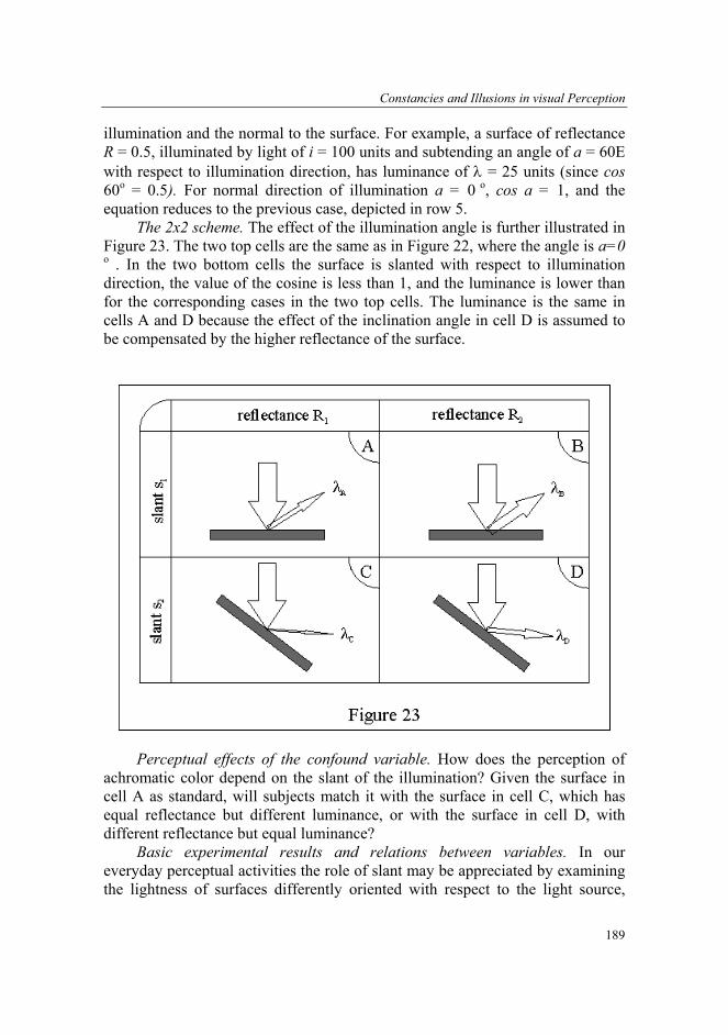
Constancies and Illusions in visual Perception
189
illumination and the normal to the surface. For example, a surface of reflectance R = 0.5, illuminated by light of i = 100 units and subtending an angle of a = 60E with respect to illumination direction, has luminance of λ = 25 units (since cos 60o = 0.5). For normal direction of illumination a = 0 o, cos a = 1, and the equation reduces to the previous case, depicted in row 5.
The 2x2 scheme. The effect of the illumination angle is further illustrated in Figure 23. The two top cells are the same as in Figure 22, where the angle is a=0
o . In the two bottom cells the surface is slanted with respect to illumination direction, the value of the cosine is less than 1, and the luminance is lower than for the corresponding cases in the two top cells. The luminance is the same in cells A and D because the effect of the inclination angle in cell D is assumed to be compensated by the higher reflectance of the surface.
Perceptual effects of the confound variable. How does the perception of
achromatic color depend on the slant of the illumination? Given the surface in cell A as standard, will subjects match it with the surface in cell C, which has equal reflectance but different luminance, or with the surface in cell D, with different reflectance but equal luminance?
Basic experimental results and relations between variables. In our everyday perceptual activities the role of slant may be appreciated by examining the lightness of surfaces differently oriented with respect to the light source,
Dejan Todorović
190
such as two adjoining walls. People generally perceive such surfaces as having the same achromatic color, but may note at the same time that one surface receives higher illumination than the other. Such a percept is an example of lightness constancy with respect to slant. However, when this setup is observed under reduction conditions, that is, through a hole that allows only the of view a part of the common edge of the two walls and portions of their adjoining regions, then the percept is different. One then sees two abutting fields of clearly different lightness; furthermore the two fields are misperceived to be coplanar (Rock, 1975; see also Gelb, 1932). Such results suggest a coupling of perceived slants and perceived achromatic colors, with the luminances held constant. Several studies have confirmed such a relationship (Hochberg & Beck, 1954; Beck, 1965; Flock & Freedberg, 1970), with especially strong effects reported by Gilchrist (1980).
(b) Achromatic color illusions. Illusions of achromatic color involve surfaces with equal reflectance and
luminance that are perceived to have different achromatic color, or surfaces with different reflectance and luminance that are perceived to have equal achromatic color. These displays involve reflecting surfaces lying in the same plane, viewed under equal illumination and equal illumination angle; thus these variables do not act as confounds. Note that in many studies such displays are simulated by various combinations of emissive surfaces, slanted surfaces, and several sources of illuminations; however, such setups generally give the impression of coplanar reflecting surfaces under equal illumination.
The classical example of a lightness illusion is simultaneous lightness contrast (Hess & Pretori, 1894/1970; Wallach, 1948; Heinemann, 1972; Gilchrist 1988; Whittle, 1994a,b). It basically involves a patch of one luminance and reflectance surrounded by a patch of different luminance and reflectance. In Figure 24 the central square has one level of luminance in cells A and C in the left column, and a somewhat lower level of luminance in cells B and D in the right column. The surround has high luminance in cells A and B in the top row, and low luminance in cells C and D in the bottom row.
The perceptual effect of interest here concerns the comparison of lightness of central patches. Comparison of row cells illustrates the effect of luminance on lightness. Comparison of column cells shows that patches of equal luminance and reflectance may appear differently light: the square in cell A, with a bright surround, appears darker than the square in cell C, with a dark surround; the same is true for cells B and D. Conversely, the squares in cells A and D have approximately the same lightness: the perceptual effects of the differences of their own interior luminance are approximately compensated by the effects of

Constancies and Illusions in visual Perception
191
the differences of their surrounds. The difference in luminance of central squares that appear equally light is a measure of the strength of the effect of the surround.
Another lightness illusion is presented in Figure 25. Cell A contains two
squares of equal luminance on a homogeneous background. Cell B also contains two squares on a homogeneous background, but the right-hand square is slightly less luminant. In cell C, the two squares of cell A are placed on a black-and-white background, whereas in cell D the same background is used for the two squares of cell B.
The two squares in cell C do not appear equally light although they are equally luminant; instead, the right-hand square appears lighter. This phenomenon is an example of White's effect (White, 1979; White & White, 1985; Kingdom & Moulden (1991); Špehar, Gilchrist & Arend, 1995). In contrast, the two differently luminant squares in cell D appear, if not exactly equally light, at least more similar in lightness than the equiluminant squares in cell C. Note an important structural difference between simultaneous contrast and White's effect: in simultaneous contrast one target square is completely surrounded by white and the other by black; in White's effect, both target squares border on both white and black surrounding regions, and the borders are of equal length.

Dejan Todorović
192
The two illusions presented above were described as illusions of lightness.
In most studies of achromatic color illusions the difference between lightness and brightness is not emphasized. However, there is no reason to expect a different structure of results with lightness and brightness instructions, because the displays are perceived as being under equal illumination.
There are many other achromatic color illusions. They include the Mach bands (Mach, 1865; Ratliff, 1965), the Ehrenstein illusion (Ehrenstein, 1941; Spillmann, Fuld, & Gerrits, 1976), lightness assimilation (Helson, 1961), the Craik-O'Brien-Cornsweet effect (Cornsweet, 1970; Burr, 1987; Todorović, 1987), the Hermann grid (Hermann, 1870; Spillmann, 1994), the Koffka-Benussi ring (Metzger, 1975), achromatic neon color (Bressan, 1993), and others (e.g. Spillmann & Levine, 1971; McCourt, 1982; Adelson, 1993; Todorović, 1997).
2. Perception of chromatic color Distal, proximal, and phenomenal chromatic color will be considered.
Distal chromatic color is the spectral distribution of reflectance of chromatic surfaces. In contrast to all discussed geometric attributes, as well as achromatic color, chromatic color is neither a scalar nor a vector variable but a functional variable, that is, it cannot, in principle, be specified with a single number or several numbers, but by an infinity of numbers, that is, a function. This function
Constancies and Illusions in visual Perception
193
is denoted here as R(w) and specifies, for each wavelength w, the fraction of light that the surface reflects at that wavelength.
Proximal chromatic color is the spectral distribution of luminance, denoted here as λ (w). It specifies, for each wavelength, the amount of light that arrives at a retinal locus in unit time.
The perceived or phenomenal colors of chromatic surfaces have a more complex structure than for achromatic surfaces. Three phenomenal attributes are usually distinguished, called hue, lightness, and saturation. In the following I will mainly consider the attribute of hue. Two variants of perceived chromatic color can in principle be distinguished, perceived distal and perceived proximal chromatic color.
(a) Chromatic color constancy Target, proximal, and confound variable. Three functional variables and
their relations are listed in row 7 of Figure 8, using simplified and somewhat artificial examples of spectral distributions. The mathematical relation between these three variable is the complete functional analogue of the corresponding achromatic case, and is given by λ(w) = R(w) i(w). Thus for any concrete value of wavelength w, the luminance at that wavelength is given as the product of surface reflectance at that wavelength and illumination at that wavelength. Therefore, as in the achromatic case, the proximal variable, the luminance spectral distribution reflected from a surface, is affected not only by the distal variable, the reflectance spectral distribution of that surface, but also by a confound variable, the spectral distribution of the illumination.
The way the above formula works in a simple case is also sketched in row 7. It contains a graphical depiction of the effects of the three variables as well as the corresponding three functions. The independent, x-axis variable is in all three cases the wavelength w of light. The spectral distribution of illumination, i(w), is, for simplicity, assumed homogeneous, that is, it contains light of equal intensity at all wavelengths. The reflectance spectral distribution has the shape of an inverted-U function. Consequently, the luminance spectral distribution also has the same shape, because it results from the multiplication of the reflectance spectral distribution by a constant number. This situation very roughly corresponds to a greenish surface illuminated by daylight.
The 2x2 scheme. The relations between the three variables are further discussed in Figure 26. Note that cell A depicts the same state of affairs as row 7 in Figure 8. Cells A and C involve a surface with an inverted-U (parabolical) reflectance spectral distribution, whereas cells B and D involve a surface with a negatively sloped linear reflectance spectral distribution. On the other hand, cells A and B depict constant illumination at all wavelengths, whereas cells C and D

Dejan Todorović
194
depict a positively sloped linear illumination spectral distribution. In all cells the luminance distribution is the product of the illumination distribution and the reflectance distribution.
Note that the shapes of the luminance distributions in cells A and B are the same as the shapes of the reflectance distributions; this is because the illumination distribution is constant. In contrast, all three distributions in cells C and D have different shapes. Consider first cell C. Since the reflectance is zero at the endpoints of the distribution, the luminance must also be zero at those points. The reflectance distribution is symmetrical about its midpoint, but the illumination distribution is asymmetrical, so that the luminance distribution is also asymmetrical. The exact shape of the luminance distribution is given by the product of the linear function and the parabolic function. In cell D, the shape of the luminance distribution is given by the product of two linear functions of opposite slope, and is the same as in cell A.
Perceptual effect of the confound variable. The preceding analysis is
purely photometric. The crucial perceptual issue is the appearance of surfaces in question. Given the surface in cell A as standard, will it be matched with the surface in cell C, which has the same reflectance distribution but different luminance distribution, or the surface in cell D with a different reflectance distribution but same luminance distribution?

Constancies and Illusions in visual Perception
195
Two types of phenomenal variables. Similar to the achromatic case, two types of phenomenal chromatic colors may be distinguished. The first type can be called 'perceived distal chromatic color' or 'perceived chromatic reflectance'. It refers to the conscious impression of the color of object surfaces. The second type can be called 'perceived proximal chromatic color' or 'perceived chromatic luminance'. It refers to the conscious impression of the color of the light arriving at the retina from some spatial direction. This type of distal-proximal distinction has rarely been explicitly drawn in color research. Exceptions include Arend (1993, 1994), who has suggested terms 'apparent surface color', on the one hand, and 'unasserted color' or 'unattributed color' on the other, and Kuriki & Uchikawa (1996), who use the terms 'surface color' and 'apparent color' for a related distinction. The instructions that attempt to elicit matches reflecting the two types of phenomenal variables are similar to analogous instructions concerning achromatic color perception.
Presentation conditions. Many chromatic color perception studies are conducted under very restricted-cue conditions, that is, both the standard and the comparison color field are presented as patches of light on dark, homogeneous achromatic backgrounds. Many other studies involve slightly more complex stimuli, involving both center and surround portions. There are also studies using more differentiated stimuli, consisting of random arrangements of rectangles ('mondrians'). More natural conditions, involving complexities such as 3-D layouts, multiple light sources, or shadows, are rarely used, because of problems of exact specifications of stimuli.
Basic experimental results. With completely reduced-cue conditions, matches are performed in terms of luminance distributions. That is, two isolated fields of light are perceived to have equal chromatic color when the compositions of light arriving from them at the retina are equal. However, under laboratory conditions, isolated light fields of physically very different compositions may also have equal perceived chromatic color, provided that they have equal effects on the retinal cones; this is the phenomenon of metamerism, which will not be considered here.
Two light fields of equal distal chromatic color under equal illumination may not have equal perceived chromatic color if their immediate surrounds are different. This is 'simultaneous color contrast', a chromatic color illusion phenomenon, which will be considered in the next section.
Of main interest in the present section are conditions in which surfaces are viewed under different illumination. Everyday observations suggest that when a surface is viewed freely, as a part of a more articulated display, its perceived chromatic color in general tends to stay the same in spite of changes in the composition of illumination, say from daylight to artificial

Dejan Todorović
196
light. Thus approximate chromatic color constancy obtains, that is, perceptual matches are made in terms of reflectance distributions. Experimental studies indicate that, in general, chromatic color constancy is a less stable and dependable phenomenon than achromatic color constancy. Furthermore, whereas constancy may hold very well for some particular combinations of surface colors and illumination colors, it may fail drastically for some other combinations (Katz, 1935; Wallach & Galloway, 1946; Helson, Judd, & Warren, 1952; Worthey, 1985; Arend & Reeves, 1986; Blackwell & Buchsbaum, 1988; Valberg & Lange-Malecki, 1990; Brainard & Wandell, 1992; Arend, 1993; Kuriki & Uchikawa, 1996). One problem is that the number of combinations of surface colors and illumination colors is huge, and that most experiments have sampled only a small portion of the possible stimulus space.
In addition to perceived distal and proximal chromatic color, there is a third phenomenal variable of potential relevance in chromatic color studies. This variable is 'perceived chromatic illumination'. It corresponds to the conscious impression of the color of illumination. Everyday observations suggest that we are sometimes sensitive to the chromatic difference of daylight and various kinds of artificial lighting, for example when we experience them in close spatial arrangement or temporal succession. However, this variable has attracted little experimental interest. A chromatic analogue of the albedo hypothesis, which would suggest a coupling of perceived distal chromatic color and perceived chromatic illumination, with the luminance distribution held constant, appears also to have escaped attention.
(b) Chromatic color illusions Illusions of perception of chromatic color arise when surfaces of equal
distal and proximal chromatic color have different perceived color, or vice versa, with illumination held constant. The classical example of such an effect is simultaneous color contrast, one version of which is schematically illustrated in Figure 27. The stimuli involve a central region and a surround. Cell A depicts a situation with a central region that emits monochromatic light of 580 nm, and an achromatic surround. Cell B involves a central region with light of somewhat longer wavelength (600 nm) on the same surround as in cell A. Cells C and D involve the same center regions as cells A and B, respectively, but the surrounds here consist of monochromatic light of 700 nm.

Constancies and Illusions in visual Perception
197
The perceptual effects concern the appearance of center regions. The
phenomenal color generally corresponding to light of 580 nm viewed on an achromatic surround is yellow (cell A). Light of longer wavelength on the same surround is perceived as reddish yellow (cell B). When the same lights are viewed on different surrounds they look different. Viewed on a surround consisting of light of 700 nm, which is perceived as red, light of 580 nm appears as a somewhat greenish yellow (cell C). This shift towards green is also induced in the 600 nm field (cell D) and is assumed to approximately cancel the reddish tinge, so that the surface appears more purely yellow, similar to cell A. The difference in the spectral composition of the central regions that look similar is a measure of the strength of the effect. Note that the concrete wavelengths used in these examples serve only for illustration purposes; however, the structure of the general trend of simultaneous color contrast phenomena is well established in empirical studies (Ware & Cowan, 1982; Krauskopf, Zaidi, & Mandler, 1986).
There are a number of other chromatic color illusions, most of them variants of corresponding achromatic color illusions. They include the chromatic Cornsweet effect (Arend, 1973; Ware & Cowan, 1983), chromatic Mach bands (Ware & Cowan, 1987), chromatic assimilation (von Bezold, 1874; Hurvich, 1981), the chromatic White's effect (Munker, 1970; Kingdom & Moulden,

Dejan Todorović
198
1989), the chromatic neon color illusion (van Tuijl, 1975; Redies & Spillmann, 1981), the chromatic Koffka-Benussi ring (Koffka, 1935), and others.
PART IV: SUMMARY AND CLOSING COMMENTS 1. Summary In this paper a systematic expository framework for visual constancies and
illusions is presented and illustrated with many examples. Starting from the notions of distal, proximal, and phenomenal visual domains, the relations of concordance and discordance between pairs of domains are defined, followed by the definitions of four visual modes (concordant, proximal, constancy, illusion) as particular constellations of concordance-discordance relations between all three domains. Constancies and illusions are characterized by proximal-phenomenal discordance.
Attributes of entities of visual domains are divided into the geometric and the photometric class, and into the intrinsic and the extrinsic class. Among geometric attributes, size and shape (involving extension) are intrinsic, and location and orientation (involving position) are extrinsic. Among photometric attributes, reflectance is intrinsic and illumination is extrinsic.
For each kind of visual attribute, two corresponding phenomenal attributes are described. The first is distally focused, involving the conscious impression of the distal attribute, and the second is proximally oriented, involving the conscious impression of the proximal attribute. The need for explicitly distally or proximally focused matching instructions is stressed.
Examples from studies of perception of size, shape, direction, orientation, and achromatic and chromatic color perception are discussed, involving all four visual modes, with the main stress on constancies and illusions. The presentation emphasizes the formal similarities of the structure of these phenomena.
All constancy examples involve a distal target variable, the corresponding proximal variable, and a confound variable that affects the proximal variable in addition to the target variable. In cases of size and color perception, two confound variables were noted, with corresponding two types of constancies. The relations between the variables are presented in analytical form as well as through a simple 2x2 scheme, demonstrating the effects of the target variable and the confound variable on the proximal variable, and showing how different combinations of values of the two independent variables may result in the same value of the dependent, proximal variable. Experimental results present the following overall picture. Under reduced-cue conditions subjects, in general, match objects in terms of values of proximal variables. Under full-cue

Constancies and Illusions in visual Perception
199
conditions, and with distally oriented instructions, the matches are, in general, more or less in accord with the values of the distal variable. Such results are standard examples of perceptual constancies. However, often results are reported in which the values of the attribute of the perceptually matching comparison stimuli are larger ('overconstancy') or smaller ('underconstancy') than the corresponding values of the standard stimuli. With proximally oriented instructions, matching values exhibit a distinct tendency towards proximal matching; however, the results are often inaccurate and show more variability than with distally oriented instructions. Finally, salient cases are pointed out in which relations between phenomenal variables tend to take a form qualitatively similar to the relation of the corresponding non-phenomenal variables.
Visual illusions also involve perceptual effects of confound variables; however, their variation does not affect the proximal variable but the phenomenal variable. Most illusion-inducing confound variables are contextual variables. Their influence is illustrated through a 2x2 scheme, which also shows how different combinations of values of the target and confound variable may induce equal values of the phenomenal variables. Experiments which involve such combinations, establish the strength of illusions.
2. Closing comments Although the main focus of the paper concerns the structural similarities
between various constancies and illusions, there are also important differences between different kinds of perceptual variables. For example, the relation between distal and phenomenal chromatic color is quite different from the relation of distal and phenomenal geometric attributes because of the specific nature of the transformation of the luminance spectral distribution by the retinal rods and cones. Also, the phenomena of perception of location and orientation are different from the other attributes in that they explicitly involve reference frames, and that the confound variables of gaze direction and eye orientation are not external but postural. Furthermore, different kinds of phenomenal attributes exhibit different kinds of salient or canonical values. In chromatic color perception, the canonical hues are red, green, yellow and blue, and in achromatic color perception the canonical values are black and white. Canonical orientations are horizontal and vertical, and the canonical egocentric direction is straight ahead. In shape perception, examples of canonical shapes could be the straight line, the circle, the square, and other regular geometric bodies. Size perception appears to lack canonical values.
The difference between constancies and illusions was portrayed here as a formal difference in the structure of concordance-discordance relations between

Dejan Todorović
200
three perceptual domains. However, in the actual research praxis, there are many other differences between the studies of constancies and illusions. For example, researchers interested in constancies are often guided by a general approach that insists on the overall veridicality of perception and the reliability of the knowledge of the outside world gained by the senses. In contrast, students of illusions appear to be more scientifically motivated by the many curious discrepancies between reality and appearance that can be induced even by very simple stimulus manipulations. Such differences in basic frameworks have created two partly divergent research traditions, the existence of which may make the goal of a more unified perceptual theory harder to attain.
The discussions of various theories of constancies and illusions are deliberately left out of scope of the present paper. It must be pointed out that the common structure of constancies and illusions as phenomena, developed here, does not at all logically implicate a common, single type of explanations of these phenomena. Phenomena which are similar according to some criteria, might, and sometimes do, have different types explanations, and vice versa. On the other hand, the existence of common structure of a set of phenomena does tend to suggest similarly structured explanations. For example, in one approach, all constancies are explained by a 'taking-into-account mechanism', in which the perception of the distal target variable is based upon the corresponding proximal variable, with the confound variable being 'taken into account' (Epstein 1973). In contrast, in other approaches constancies are based on relative values of proximal variables of two or more stimuli (see Rock, 1975), or on higher-order optical variables (Gibson, 1979). Some theories of illusions claim that many of them can be explained as byproducts of misapplied constancy mechanisms (Tausch, 1954; Gregory, 1963; Gillam, 1980). Others stipulate excitatory and inhibitory interactions between neural mechanisms. To what extent these general approaches are successful in the explanations of the phenomena reviewed here can only be decided on the basis of a case by case confrontation of theories with concrete data on concrete phenomena. Out of such confrontations, one or more dependable unifying perceptual explanatory principles might emerge in the end.

Constancies and Illusions in visual Perception
201
REFERENCES
Adelson, E.H. (1993). Perceptual organization and the judgement of brightness. Science, 262, 2042-2044
Arend, L. (1973). Spatial differential and integral operations in human vision: Implications of stabilized retinal image fading. Psychological Review, 80,374-395.
Arend, L.E. (1993). How much does illuminant color affect unattributed colors? Journal of the Optical Society of America, A, 10, 2134-2147.
Arend, L.E. (1994). Surface colors, illumination, and surface geometry: intrinsic-image models of human color perception. In A. Gilchrist (Ed.) Lightness, brightness, and transparency. Hillsdale: LEA.
Arend, L. & Goldstein, R. (1987). Simultaneous constancy, lightness, and brightness. Journal of the Optical Society of America, A, 7, 1929-1936.
Arend, L.E. & Reeves, A. (1986). Simultaneous color constancy. Journal of the Optical Society of America, A, 3, 1743-1751.
Arend, L.E. & Òpehar, B. (1993a). Lightness, brightness, and brightness contrast: 1. Illuminance variation. Perception & Psychophysics, 54, 446-456.
Arend, L.E. & Òpehar, B. (1993b). Lightness, brightness, and brightness contrast: 1. Reflectance variation. Perception & Psychophysics, 54, 457-468.
Baird, J.C. & Biersdorf, W.R. (1967). Quantitative functions for size and distance judgements. Perception & Psychophysics, 2, 161-166.
Baird, J.C. & Wagner, M. (1991). Transformation theory of size judgement. Journal of experimental psychology: Human perception and performance, 17, 852-864.
Beck, J. (1961). Judgements of surface illumination and lightness. Journal of Experimental Psychology, 61, 368-375.
Beck, J. (1965). Apparent spatial position and the perception of lightness. Journal of Experimental Psychology, 69, 170-179.
Beck, J. (1972). Surface color perception. Ithaca: Cornell University Press. Beck, J. & Gibson, J.J. (1955). The relation of apparent shape to apparent slant in
the perception of objects. Journal of Experimental Psychology, 50, 125-133. Blackwell, K.T. & Buchsbaum, G. (1988). Quantitative studies of color constancy.
Journal of the Optical Society of America, A, 5, 1772-1780. Boff, K.R., Kaufman, L, & Thomas, J.P. (1986). Handbook of Perception and
Human Performance. Vols I and II. New York: Wiley. Bonato, F. & Gilchrist, A. (1994). The perception of luminosity on different
backgrounds and in different illuminations. Perception, 23, 991-1006. Borresen, C.R. & Lichte, W.H. (1967). Influence of instructions on degree of shape
constancy. Journal of Experimental Psychology, 74, 538-542. Brainard, D. & Wandell, B. (1992). Asymmetric color matching: how color
appearance depends on the illuminant. Journal of the Optical Society of America, A, 9, 1433-1448.
Bressan, P. (1993). Revisitation of the luminance conditions for the occurrence of the achromatic neon color spreading illusion. Perception, 54, 55-64.
Bridgeman, B. (1993). Separate visual representations for perception and for visually guided behavior. In Ellis, S.R. (Ed.), Pictorial communication in virtual and real environments, 2nd edition. London: Taylor & Francis.
Bruell, J.H. & Albee, G.W. (1955). Effect of asymmetrical retinal stimulation on the perception of the median plane. Perceptual and Motor Skills, 5, 133-139.
Burr, D.C. (1987). Implications of the Craik-O'Brien illusion for brightness perception. Vision Research, 27, 1903-1913.
Campione, F. (1977). Shape constancy: a systematic approach. Perception, 6, 97-105.

Dejan Todorović
202
Carlson, V.R. (1960). Overestimation in size constancy judgments. American Journal of Psychology, 73, 199-213.
Carlson, V.R. & Tassone, E.P. (1967). Independent size-judgements at different distances. Journal of Experimental Psychology, 73, 491-497.
Cataliotti, J. & Gilchrist, A. (1995). Local and global processes in surface lightness perception. Perception & Psychophysics, 57, 125-135.
Cohen, M.M., Ebenholtz, S.M., & Linder, B.J. (1995). Effects of optical pitch on oculomotor control and the perception of target elevation. Perception & Psychophysics, 57, 433-440.
Coren, S. & Girgus, J.S. (1978). Seeing is deceiving: The psychology of visual illusions. Hillsdale, NJ: Erlbaum.
Cornsweet, T. (1970). Visual Perception. New York: Academic Press. Cutting, J.E. & Vishton, P.M. (1995). Perceiving layout and knowing distances: the
integration, relative potency, and contextual use of different information about depth. In: W. Epstein and Rogers, S. (Eds.), Perception of space and motion. New York: Academic press.
Ebenholtz, S.M. (1977a). Determinants of the rod and frame effect: The role of retinal size. Perception & Psychophysics, 22,531-538
Ehrenstein, W. (1925). Versuche hber die Beziehung zwischen Bewegungs- und Gestalt-wahrnehmungen. Zeitschrift fhr Psychologie, 95, 305-352.
Epstein, W. (1961). Phenomenal orientation and perceived achromatic color. Journal of Psychology, 52, 51-53.
Epstein, W. (1963). Attitude of judgment and the size-distance invariance hypothesis. Journal of experimental Psychology, 66, 78-83.
Epstein, W. (1973). The process of 'taking-into-account' in visual perception. Perception, 2, 267-285.
Epstein, W. (1977). Stability and constancy in visual perception: Mechanisms and processes. New York: Wiley.
Epstein, W., Bontrager, H., & Park, J. (1962). The induction of nonveridical slant and the perception of shape. Journal of Experimental Psychology, 63, 472-479.
Epstein, W. & Landauer, A. (1969). Size and distance judgments under reduced conditions of viewing. Perception & Psychophysics, 6, 269-272.
Epstein, W. & Park, J.K. (1963). Shape constancy: Functional relationships and theoretical formulations. Psychological Bulletin, 60, 265-288.
Epstein, W., Park, J., & Casey, A. (1961). The current status of the size-distance hypothesis. Psychological Bulletin, 58, 491-514.
Eriksson, E.S. (1967a). The shape slant invariance in static perception. Scandinavian Journal of Psychology, 8, 193-208.
Eriksson, E.S. (1967b). Factors influencing two-dimensional form perception. Scandinavian Journal of Psychology, 8, 209-217.
Flock, H.R. & Freedberg, E. (1970). Perceived angle of incidence and achromatic surface color. Perception & Psychophysics, 8, 251-256.
Gelb, A. (1929). Die "Farbenkonstanz" der Sehdinge. In: A. Bethe, G.v.Bergmann, G. Embden, & A. Ellinger (Eds.), Handbuch der normalen und pathologischen Physiologie, Vol. 12., (p. 594-678). Berlin: Springer.
Gelb, A. (1932). Die Erscheinungen des simultanen Kontrastes und der Eindruck der Feldbeleuchtung. Zeitschrift fhr Psychologie, 127, 42-59.
Gibson, J.J. (1950). The Perception of the Visual World. Boston: Houghton Mifflin. Gibson, J.J. (1979). The Ecological Approach to Visual Perception. Boston, MA:
Houghton Mifflin. Gilchrist, A. (1977). Perceived lightness depends on perceived spatial arrangement?
Science, 195, 185-187.

Constancies and Illusions in visual Perception
203
Gilchrist, A. (1980). When does perceived lightness depend on perceived spatial arrangement? Perception & Psychophysics, 28, 528-537.
Gilchrist, A. (1988). Lightness contrast and failures of constancy: a common explanation. Perception & Psychophysics, 43, 415-424.
Gilchrist, A. (1994). Lightness, brightness, and transparency. Hillsdale: LEA Gilchrist, A., Delman, S., & Jacobsen, A. (1983). The classification and integration
of edges as critical to the perception of reflectance and illumination. Perception & Psychophysics, 33, 425-436.
Gillam, B. (1980). Geometrical illusions. Scientific American, 242, 86-95. Gillam, B. (1995). The perception of spatial layout from static optical information.
In: W. Epstein and Rogers, S. (Eds.), Perception of space and motion. New York: Academic press.
Gilinsky, A. (1955). The effect of attitude on the perception of size. American Journal of Psychology, 68, 173-192.
Gogel, W.C. & Mershon, D.H. (1969). Depth adjacency in simultaneous contrast. Perception & Psychophysics, 5, 13-17.
Goodenough, D.R., Nowak, A., Oltman, P.K., Cox, P.W., & Sigman, E. (1982). A visually induced body tilt in a horizontal plane. Perception & Psychophysics, 31, 268-272.
Gregory, R. (1963). Distortion of visual space as inappropriate constancy scaling. Nature, 199, 678-680.
Hastorf, A.R. Way, K.S. (1952). Apparent size with and without distance cues. Journal of General Psychology, 47, 181-188.
Heinemann, E.G. (1972). Simultaneous brightness induction. In D. Jameson & L. Hurvich (Eds.), Handbook of Sensory Physiology. Berlin: Springer.
Heggelund, P. (1992). A bidimensional theory of achromatic color vision. Vision Research, 32, 2107-2119.
Helson, H. (1963). Studies on anomalous contrast and assimilation. Journal of the Optical Society of America, 53, 179-184.
Helson, H., Judd, D.B., & Warren, M.H. (1952). Object color changes from daylight to incandescent filament illumination. Illumination Engineering, 47, 221-233.
Hering (1964). Outlines of a theory of the light sense.. (L.M. Hurvich & D. Jameson, Trans.). Cambridge, MA: Harvard University Press. (Original work published 1874).
Hermann, L. (1870). Eine Erscheinung des simultanen Contrastes. Pflhgers Archiv fhr die gesamte Physiologie, 3, 13-15.
Hess, C. & Pretori, H. (1894/1970). Quantitative investigation of the lawfulness of simultaneous brightness contrast (H. Flock & J.H. Tenney, Trans.). Perceptual and Motor Skills, 31, 947-969. (Original work published 1894).
Higashiyama, A. & Ueyama, E. (1988). The perception of vertical and horizontal distances in outdoor settings. Perception & Psychophysics, 44, 151-156.
Hill, A.L. (1972). Direction constancy. Perception & Psychophysics, 11, 175-178. Hillebrand, F. (1928). gber die scheinbare Streckenverkhrzung im indirekten Sehen.
Zeitschrift fhr Psychologie, II Abt., 59,174-196. Hochberg, J. (1971a). Perception. I. Color and shape. In J.W. Kling & L.A. Riggs
(Eds.), Woodworth & Schlosberg's Experimental Psychology, 3rd edition. New York: Holt, Rinehart and Winston.
Hochberg, J. (1971b). Perception. II. Space and motion. In J.W. Kling & L.A. Riggs (Eds.), Woodworth & Schlosberg's Experimental Psychology, 3rd edition. New York: Holt, Rinehart and Winston.
Hochberg, J. & Beck, J. (1954). Apparent spatial arrangement and perceived brightness. Journal of Experimental Psychology, 47, 263-266.

Dejan Todorović
204
Holway, A.H. & Boring, E.G. (1941). Determinants of apparent visual size with distance variant. American Journal of Psychology, 54, 21-37.
Howard, Ian. (1986). The perception of posture, self motion, and the visual vertical. In K.R. Boff, L. Kaufman, & J.P. Thomas (Eds.), Handbook of Perception and Human Performance. Vol. I. New York: Wiley.
Ittelson, W.H. (1952). The Ames demonstrations in perception. A guide to their construction and use. Princeton, N.J.: Princeton University Press.
Jenkin, N.A. (1959). a relationship between increments of distance and estimates of objective size. American Journal of Psychology, 72, 345-363.
Joynson, R.B. (1949). The problem of size and distance. Quarterly Journal of Experimental Psychology, 1, 119-135.
Joynson, R.B. (1958a). An experimental synthesis of the Associationist and Gestalt accounts of perception of size. Part I. Quarterly Journal of Experimental Psychology, 10, 65-76.
Joynson, R.B. (1958b). An experimental synthesis of the Associationist and Gestalt accounts of perception of size. Part II. Quarterly Journal of Experimental Psychology, 10, 142-154.
Joynson, R.B. & Kirk, N.S. (1960). An experimental synthesis of the Associationist and Gestalt accounts of perception of size. Part II I. Quarterly Journal of Experimental Psychology, 12, 221-230.
Joynson, R.B. & Newson, L.J. (1962). The perception of shape as a function of inclination. British Journal of Psychology, 53, 1-15.
Kaiser, P.K. (1967). Perceived shape and its dependency on perceived slant. Journal of Experimental Psychology, 75, 345-353.
Katz, D. (1935). The world of colour. (R.B. MacLeod & C.W. Fox, Trans.). London: Kegan Paul, Trench, Trubner & Co.
Kingdom, F. & Moulden, B. (1989). Corner effects in induced hue: evidence for chromatic band-pass filters. Spatial Vision, 4, 253-266.
Kingdom, F. & Moulden, B. (1991). White's effect and assimilation. Vision Research, 31, 151-159.
Koffka, K. (1935). Principles of Gestalt Psychology. New York: Harcourt Brace. Kozaki, A. & Noguchi, K. (1976). The relationship between perceived surface-
lightness and perceived illumination: a manifestation of perceptual scission. Psychological Research, 19, 1-16.
Krauskopf, J., Zaidi, Q., & Mandler, M.C. (1986). Mechanisms of simultaneous color induction. Journal of the Optical Society of America, A, 3, 1752-1757.
Kilpatrick, F.P. & Ittelson, W.H. (1953). The size-distance invariance hypothesis. Psychological Review, 60, 223-231.
Kuriki, I. & Uchikawa, K. (1996). Limitations of surface-color and apparent-color constancy. Journal of the Optical Society of America A, 13, 1622-1636.
Landauer, A.A. (1969). Influence of instructions on judgements of unfamiliar shape. Journal of Experimental Psychology, 79, 129-132.
Leibowitz, H. & Harvey, L.O. (1967). Size matching as a function of instructions in a naturalistic environment. Journal of Experimental Psychology, 74, 378-382
Levin, C.A. & Haber, R.N. (1993). Visual angle as a determinant of perceived interobject distance. Perception & Psychophysics, 54, 250-259.
Li, W. & Matin, L. (1995). Differences in influence between pitched-from-vertical lines and slanted-from-horizontal lines on egocentric localization. Perception & Psychophysics, 57, 71-83.
Lie, I. (1969). Psychophysical invariants of achromatic colour vision. I. The multidimensionality of achromatic colour experience. Scandinavian Journal of Psychology, 10, 167-175.

Constancies and Illusions in visual Perception
205
Lichte, W.H. & Borresen, C.R. (1967). Influence of instructions on degree of shape constancy .Journal of Experimental Psychology, 74, 538-542.
Lichten, W. & Lurie, S. (1950). A new technique for the study of perceived size. American Journal of Psychology, 63, 281-282.
Longvinenko, A. & Menshikova, G. (1994). Trade-off between achromatic color and perceived illumination as revealed by the use of pseudoscopic inversion of apparent depth. Perception, 23, 1007-1023.
Mach, E. (1865). Von der Wirkung der räumlichen Vertheilung des Lichtreizes auf die Netzhaut. Sitzungsberichte der kaiserlichen Akademie der Wissen-schaften. Mathematisch-naturwissenschaftliche Classe, zweite Abtheilung, 52, 303-322.
Mann, C.W., Berthelot-Berry, N.H., & Dauterive, H.J. (1949). The perception of the vertical: I. Visual and non-labyrinthine cues. Journal of Experimental Psychology, 39, 538-547.
Martius, G. (1889). Uber die scheinbare Grösse der Gegenstände und ihre Beziehung zur Grösse der Netzhautbilder. Philosophische Studien, 5, 601-617.
Matin, L. (1986). Visual localizations and eye movements. In K.R. Boff, L. Kaufman, & J.P. Thomas (Eds.), Handbook of Perception and Human Performance Vol. I. New York: Wiley.
McCourt, M. (1982). A spatial frequency dependent grating-induction effect. Vision Research, 22, 119-134.
McCready, D. (1985). On size, distance, and visual angle perception. Perception & Psychophysics, 37, 323-334.
Metzger, W. (1975). Gesetze des Sehens, 3rd. ed. Frankfurt: Kramer. Miller, E.F., Fregly, A.R., van den Brink, G., & Graybiel, A. (1965). Visual
localization of the horizontal as a function of body tilt up to +/- 90o from gravitational vertical. (NSAM-942). Pensacola: Naval School of Aviation Medicine.
Morgan, C.T. (1978). Constancy of egocentric visual direction. Perception & Psychophysics, 23, 61-68.
Munker, H. (1970). Farbige Gitter, Abbildung auf der Netzhaut und uhbertragungs-theoretische Beschreibung der Farbwahrnehmung. Habilitationsschrift, Ludwig - Maximilians - Universität, Mhnchen.
Nelson, T.M & Bartley, S.H. (1956). The perception of form in an unstructured field. Journal of General Psychology, 54, 57-63.
Newson, L.J. (1958). Some principles governing changes in the apparent lightness of test surfaces isolated from their normal backgrounds. Quarterly Journal of Experimental Psychology, 10, 82-95.
Noguchi, K. & Kozaki, A. (1985). Perceptual scission of surface-lightness and illumination: An examination of the Gelb effect. Psychological Research, 47, 19-25.
Norman, J.F., Todd, J.T., Perotti, V.J., & Tittle, J.S. (1996). The visual perception of three-dimensional length. Journal of experimental psychology: Human Perception and Performance, 22, 173-186.
Orbison, W.D. (1939). Shape as a function of the vector field. American Journal of Psychology, 52, 32-45.
Over, R. (1960). The effect of instructions on size-judgements under reduction conditions. American Journal of Psychology, 73, 599-602.
Paap, K.R. & Ebenholtz, S.M. (1976). Perceptual consequences of potentiation in the extraocular muscles: an alternative explanation to adaptation to wedge prisms. Journal of experimental psychology: Human Perception and Performance, 2, 457-468.

Dejan Todorović
206
Pokorny, J. & Smith, V.C. (1986). Colorimetry and color discrimination. In K.R. Boff, L. Kaufman, & J.P. Thomas (Eds.), Handbook of Perception and Human Performance Vol. I. New York: Wiley.
Ratliff, F. (1965). Mach bands: Quantitative studies on neural networks in the retina. San Francisco, CA: Holden-Day.
Redies, C. & Spillmann, L. (1981). The neon color effect in the Ehrenstein illusion. Perception, 10, 667-681.
Robinson, J.O. (1972). The psychology of visual illusions. London: Hutchinson University Library.
Rock, I. (1975). An introduction to perception. New York: Macmillan. Rock, I. & McDermott, W. (1964). The perception of visual angle. Acta
Psychologica, 22, 119-134. Roelofs, C.O. (1935). Optische Localisation. Archiv fur Augenheilkunde, 109, 395-
415. Schneider, B., Ehrich, D.J., Stein, R., Flaum, M., & Mangel, S. (1978). Changes in
the apparent length of lines as a function of degree of retinal eccentricity. Perception, 7, 215-223.
Sedgwick, H.A. (1986). Space perception. In K.R. Boff, L. Kaufman, & J.P. Thomas (Eds.), Handbook of Perception and Human Performance Vol. I. New York: Wiley.
Shebilske, W. (1977). Visuomotor coordination in visual direction and position constancies. In Epstein, W. (Ed.), Stability and constancy in visual perception: Mechanisms and processes. New York: Wiley.
Smith, W.M. (1953). A methodological study of size distance perception. Journal of Psychology, 35, 143-153.
Stewart, E. (1959). The Gelb effect. Journal of Experimental Psychology, 57, 235-242.
Stoper, A.E. & Cohen, M.M. (1986). Judgements of eye level in light and darkness. Perception & Psychophysics, 40, 311- 316.
Spillmann, L. (1994). The Hermann grid illusion: a tool for studying human perceptive field organization. Perception, 23, 691-708.
Spillmann, L. & Levine, J. (1971). Contrast enhancement in a Hermann grid with variable figure- ground ratio. Experimental Brain Research, 13, 547-559.
Spillmann, L., Fuld, K., & Gerrits, H.J. (1976). Brightness contrast in the Ehrenstein illusion. Vision Research, 16, 713-719.
Špehar, B., Gilchrist, A., & Arend, L. (1995). The critical role of relative luminance relations in White's effect and grating induction. Vision Research, 35, 2603-2614.
Tausch, R. (1954). Optische Täuschungen als artifizielle Effekte der Gestaltungs-prozesse von Grössen und Formenkonstanz in der naturlichen Raum-wahrnehmung. Psychologische Forschung, 44, 299-348.
Thouless, R.H. (1931a). Phenomenal regression to the real object. Part I. British Journal of Psychology, 21, 339-359.
Thouless, R.H. (1931b). Phenomenal regression to the real object. Part II. British Journal of Psychology, 22, 1-30.
Todorović, D. (1997). Lightness and junctions. Perception, 26, 379-394. Todorović, D. (1987). The Craik-O'Brien-Cornsweet effect: New varieties and their
theoretical implications. Perception & Psychophysics, 42, 545-560. Toye, R.C. (1986). The effect of viewing position on the perceived layout of space.
Perception & Psychophysics, 40, 85-92. Valberg, A. & Lange-Malecki, B. (1990). 'Color constancy' in Mondrian patterns: a
partial camcellation of physical chromaticity shifts by simultaneous contrast. Vision Research, 30, 371-380.
Constancies and Illusions in visual Perception
207
vanTuijl, H.F.J.M. (1975). A new visual illusion: Neonlike color spreading and complementary color induction between subjective contours. Acta Psychologica, 39, 441-445.
Wagner, M. (1985). The metric of visual space. Perception & Psychophysics, 38, 483-495.
Wallach, H. (1948). Brightness constancy and the nature of achromatic colors. Journal of Experimental Psychology, 38, 310-324.
Wallach, H. (1976). On Perception. New York: Quadrangle. Wallach, H. & Galloway, A. (1946) Constancy of colored objects in colored
illumination. Journal of Experimental Psychology, 36, 119-126. Ware, C. & Cowan, W.B. (1982). Changes in perceived color due to chromatic
interactions. Vision Research, 22, 1353-1362. Ware, C. & Cowan, W.B. (1983). The chromatic Cornsweet effect. Vision Research,
23, 1075-1077. Ware, C. & Cowan, W.B. (1987). Chromatic Mach bands: Behavioral evidence for
lateral inhibition in human color vision. Perception & Psychophysics, 41, 173-178.
Welch, R.B. & Post, R.B. (1966). Accuracy and adaptation of reaching and pointing in pitched visual environments. Perception & Psychophysics, 58, 383-389.
Werner, J.H., Wapner, S., & Bruell, J.H. (1953). Experiments on sensory-tonic field theory of perception: VI. The effect of position of head, eyes, and of object on the position of the apparent median plane. Journal of Experimental Psychology, 46, 300-307.
White, M. (1979). A new effect of pattern on perceived lightness. Perception, 8, 413-416.
White, M. & White, T. (1985). Counterphase lightness induction. Vision Research, 25, 1331-1335.
Whittle, P. (1994a). The psychophysics of contrast brightness. In A. Gilchrist (Ed.) Lightness, brightness, and transparency. Hillsdale: LEA.
Whittle, P. (1994b). Contrast brightness and ordinary seeing. In A. Gilchrist (Ed.) Lightness, brightness, and transparency. Hillsdale: LEA.
Witkin, H.A. & Asch, S.E. (1948). Studies in space orientation IV. Further experiments on perception of the upright with displaced visual fields. Journal of Experimental Psychology, 38, 762-782.
Woodworth, R.S. & Schlosberg, H. (1954). Experimental Psychology (2nd ed.). New York: Holt.
Worthey, J.A. (1985). Limitations of color constancy. Journal of the Optical Society of America, A, 2, 1014-1026.
Wundt, W. (1898). Die geometrisch-optischen Täuschungen. Abhandlungen der mathematisch-physischen Classe der Königlich Sächsischen Gesellschaft der Wissenschaften, 42, 55-178.
Wyszecki, G. (1986). Color appearance. In K.R. Boff, L. Kaufman, & J.P. Thomas (Eds.), Handbook of Perception and Human Performance Vol. I. New York: Wiley.