const. mgmt. chp. 11 - advanced scheduling techniques

8/14/2019 Const. Mgmt. Chp. 11 - Advanced Scheduling Techniques

http://slidepdf.com/reader/full/const-mgmt-chp-11-advanced-scheduling-techniques 1/27

11. Advanced Scheduling Techniques

11.1 Use of Advanced Scheduling Techniques

Construction project scheduling is a topic that has received extensive research over anumber of decades. The previous chapter described the fundamental scheduling techniqueswidely used and supported by numerous commercial scheduling systems. A variety of special techniques have also been developed to address specific circumstances or problems.With the availability of more powerful computers and software, the use of advancedscheduling techniques is becoming easier and of greater relevance to practice. In thischapter, we survey some of the techniques that can be employed in this regard. Thesetechniques address some important practical problems, such as:

scheduling in the face of uncertain estimates on activity durations, integrated planning of scheduling and resource allocation, scheduling in unstructured or poorly formulated circumstances.

A final section in the chapter describes some possible improvements in the projectscheduling process. In Chapter 14, we consider issues of computer based implementationof scheduling procedures, particularly in the context of integrating scheduling with otherproject management procedures.

Back to top

11.2 Scheduling with Uncertain Durations

Section 10.3 described the application of critical path scheduling for the situation in which

activity durations are fixed and known. Unfortunately, activity durations are estimates of the actual time required, and there is liable to be a significant amount of uncertaintyassociated with the actual durations. During the preliminary planning stages for a project,the uncertainty in activity durations is particularly large since the scope and obstacles to theproject are still undefined. Activities that are outside of the control of the owner are likelyto be more uncertain. For example, the time required to gain regulatory approval forprojects may vary tremendously. Other external events such as adverse weather, trenchcollapses, or labor strikes make duration estimates particularly uncertain.

Two simple approaches to dealing with the uncertainty in activity durations warrant somediscussion before introducing more formal scheduling procedures to deal with uncertainty.First, the uncertainty in activity durations may simply be ignored and scheduling doneusing the expected or most likely time duration for each activity. Since only one durationestimate needs to be made for each activity, this approach reduces the required work insetting up the original schedule. Formal methods of introducing uncertainty into thescheduling process require more work and assumptions. While this simple approach mightbe defended, it has two drawbacks. First, the use of expected activity durations typicallyresults in overly optimistic schedules for completion; a numerical example of this optimismappears below. Second, the use of single activity durations often produces a rigid,



inflexible mindset on the part of schedulers. As field managers appreciate, activitydurations vary considerable and can be influenced by good leadership and close attention.As a result, field managers may loose confidence in the realism of a schedule based uponfixed activity durations. Clearly, the use of fixed activity durations in setting up a schedulemakes a continual process of monitoring and updating the schedule in light of actual

experience imperative. Otherwise, the project schedule is rapidly outdated.

A second simple approach to incorporation uncertainty also deserves mention. Manymanagers recognize that the use of expected durations may result in overly optimisticschedules, so they include a contingency allowance in their estimate of activity durations.For example, an activity with an expected duration of two days might be scheduled for aperiod of 2.2 days, including a ten percent contingency. Systematic application of thiscontingency would result in a ten percent increase in the expected time to complete theproject. While the use of this rule-of-thumb or heuristic contingency factor can result inmore accurate schedules, it is likely that formal scheduling methods that incorporateuncertainty more formally are useful as a means of obtaining greater accuracy or inunderstanding the effects of activity delays.

The most common formal approach to incorporate uncertainty in the scheduling process isto apply the critical path scheduling process (as described in Section 10.3) and then analyzethe results from a probabilistic perspective. This process is usually referred to as the PERTscheduling or evaluation method. [1] As noted earlier, the duration of the critical pathrepresents the minimum time required to complete the project. Using expected activitydurations and critical path scheduling, a critical path of activities can be identified. Thiscritical path is then used to analyze the duration of the project incorporating the uncertaintyof the activity durations along the critical path. The expected project duration is equal tothe sum of the expected durations of the activities along the critical path. Assuming thatactivity durations are independent random variables, the variance or variation in theduration of this critical path is calculated as the sum of the variances along the critical path.

With the mean and variance of the identified critical path known, the distribution of activity durations can also be computed.

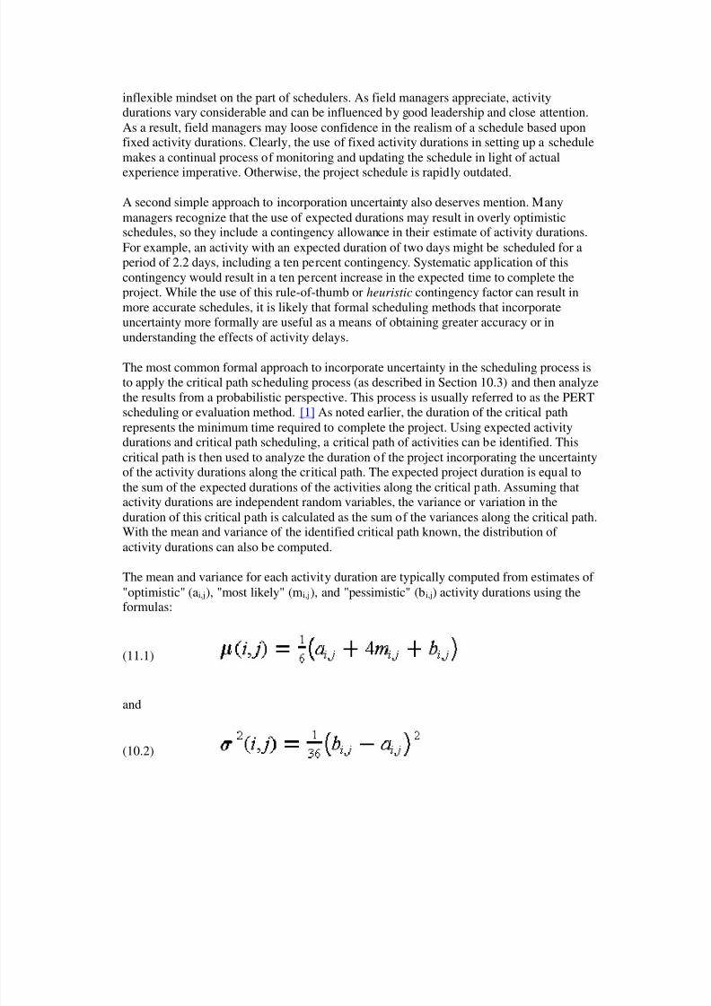
The mean and variance for each activity duration are typically computed from estimates of "optimistic" (ai,j), "most likely" (mi,j), and "pessimistic" (bi,j) activity durations using theformulas:

(11.1)

and

(10.2)



where and are the mean duration and its variance, respectively, of anactivity (i,j). Three activity durations estimates (i.e., optimistic, most likely, and pessimisticdurations) are required in the calculation. The use of these optimistic, most likely, andpessimistic estimates stems from the fact that these are thought to be easier for managers to

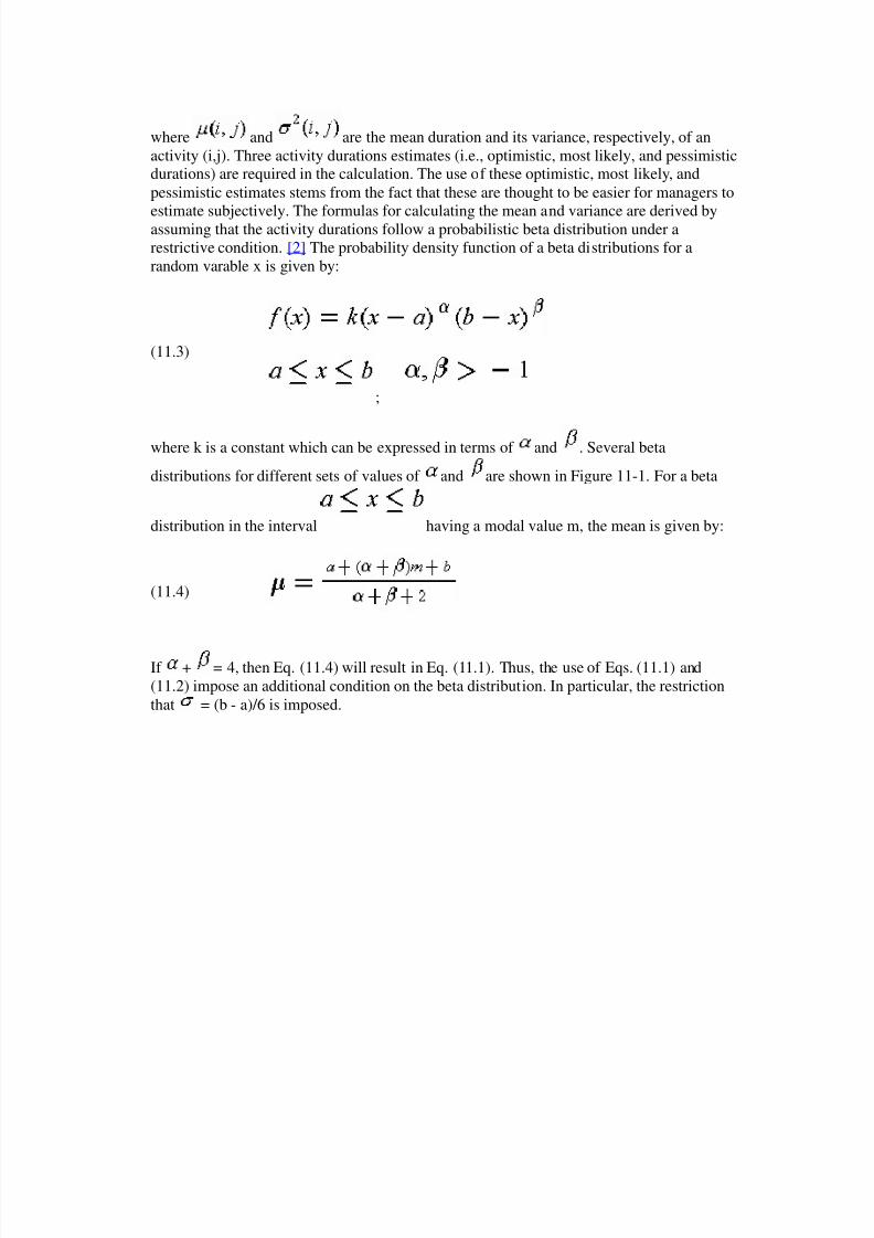
estimate subjectively. The formulas for calculating the mean and variance are derived byassuming that the activity durations follow a probabilistic beta distribution under arestrictive condition. [2] The probability density function of a beta distributions for arandom varable x is given by:

(11.3)

;

where k is a constant which can be expressed in terms of and . Several beta

distributions for different sets of values of and are shown in Figure 11-1. For a beta

distribution in the interval having a modal value m, the mean is given by:

(11.4)

If + = 4, then Eq. (11.4) will result in Eq. (11.1). Thus, the use of Eqs. (11.1) and(11.2) impose an additional condition on the beta distribution. In particular, the restrictionthat = (b - a)/6 is imposed.



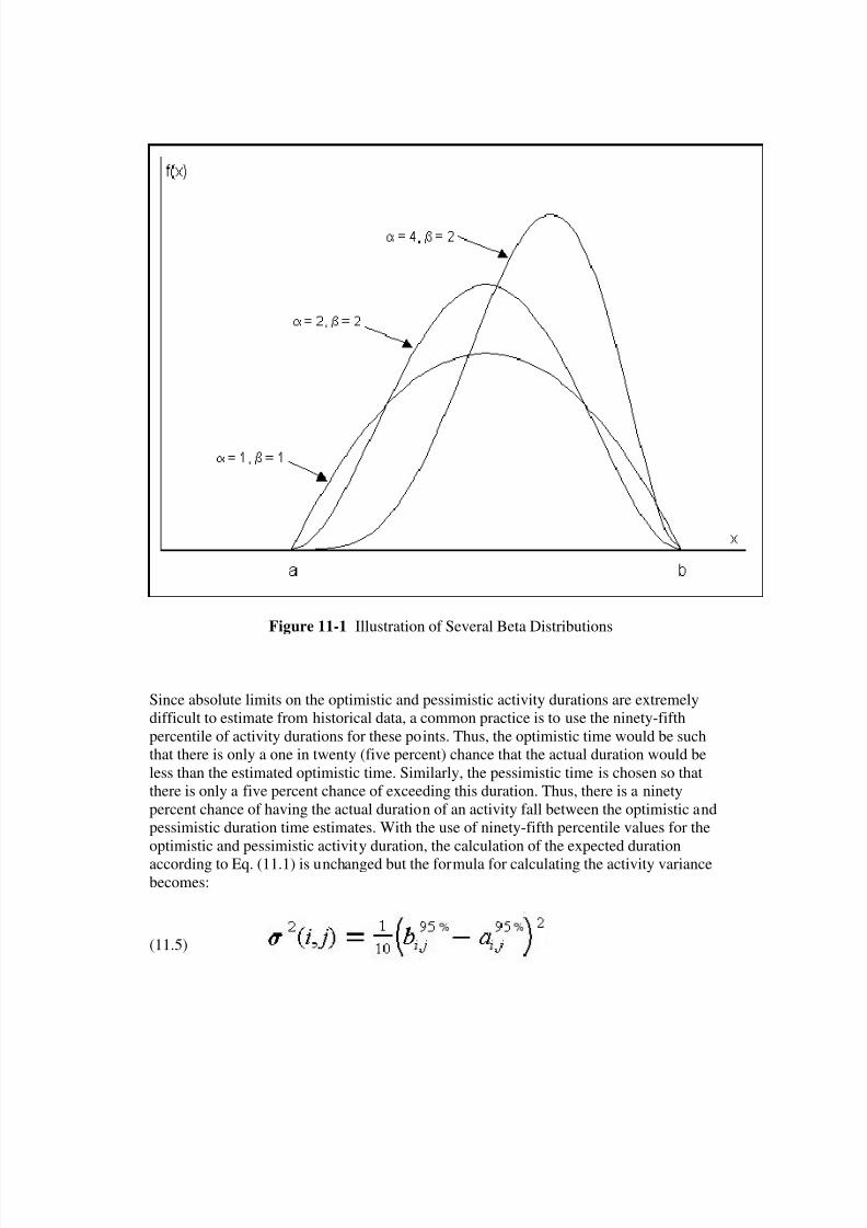
Figure 11-1 Illustration of Several Beta Distributions

Since absolute limits on the optimistic and pessimistic activity durations are extremelydifficult to estimate from historical data, a common practice is to use the ninety-fifthpercentile of activity durations for these points. Thus, the optimistic time would be suchthat there is only a one in twenty (five percent) chance that the actual duration would beless than the estimated optimistic time. Similarly, the pessimistic time is chosen so thatthere is only a five percent chance of exceeding this duration. Thus, there is a ninetypercent chance of having the actual duration of an activity fall between the optimistic andpessimistic duration time estimates. With the use of ninety-fifth percentile values for theoptimistic and pessimistic activity duration, the calculation of the expected duration

according to Eq. (11.1) is unchanged but the formula for calculating the activity variancebecomes:

(11.5)



The difference between Eqs. (11.2) and (11.5) comes only in the value of the divisor, with36 used for absolute limits and 10 used for ninety-five percentile limits. This differencemight be expected since the difference between b i,j and ai,j would be larger for absolutelimits than for the ninety-fifth percentile limits.

While the PERT method has been made widely available, it suffers from three majorproblems. First, the procedure focuses upon a single critical path, when many paths mightbecome critical due to random fluctuations. For example, suppose that the critical path withlongest expected time happened to be completed early. Unfortunately, this does notnecessarily mean that the project is completed early since another path or sequence of activities might take longer. Similarly, a longer than expected duration for an activity noton the critical path might result in that activity suddenly becoming critical. As a result of the focus on only a single path, the PERT method typically underestimates the actualproject duration.

As a second problem with the PERT procedure, it is incorrect to assume that mostconstruction activity durations are independent random variables. In practice, durations are

correlated with one another. For example, if problems are encountered in the delivery of concrete for a project, this problem is likely to influence the expected duration of numerousactivities involving concrete pours on a project. Positive correlations of this type betweenactivity durations imply that the PERT method underestimates the variance of the criticalpath and thereby produces over-optimistic expectations of the probability of meeting aparticular project completion deadline.

Finally, the PERT method requires three duration estimates for each activity rather than thesingle estimate developed for critical path scheduling. Thus, the difficulty and labor of estimating activity characteristics is multiplied threefold.

As an alternative to the PERT procedure, a straightforward method of obtaining

information about the distribution of project completion times (as well as other scheduleinformation) is through the use of Monte Carlo simulation. This technique calculates sets of artificial (but realistic) activity duration times and then applies a deterministic schedulingprocedure to each set of durations. Numerous calculations are required in this process sincesimulated activity durations must be calculated and the scheduling procedure applied manytimes. For realistic project networks, 40 to 1,000 separate sets of activity durations mightbe used in a single scheduling simulation. The calculations associated with Monte Carlosimulation are described in the following section.

A number of different indicators of the project schedule can be estimated from the resultsof a Monte Carlo simulation:

Estimates of the expected time and variance of the project completion. An estimate of the distribution of completion times, so that the probability of

meeting a particular completion date can be estimated. The probability that a particular activity will lie on the critical path. This is of

interest since the longest or critical path through the network may change as activitydurations change.



The disadvantage of Monte Carlo simulation results from the additional information aboutactivity durations that is required and the computational effort involved in numerousscheduling applications for each set of simulated durations. For each activity, thedistribution of possible durations as well as the parameters of this distribution must bespecified. For example, durations might be assumed or estimated to be uniformly

distributed between a lower and upper value. In addition, correlations between activitydurations should be specified. For example, if two activities involve assembling forms indifferent locations and at different times for a project, then the time required for eachactivity is likely to be closely related. If the forms pose some problems, then assemblingthem on both occasions might take longer than expected. This is an example of a positivecorrelation in activity times. In application, such correlations are commonly ignored,leading to errors in results. As a final problem and discouragement, easy to use softwaresystems for Monte Carlo simulation of project schedules are not generally available. This isparticularly the case when correlations between activity durations are desired.

Another approach to the simulation of different activity durations is to develop specificscenarios of events and determine the effect on the overall project schedule. This is a type

of "what-if" problem solving in which a manager simulates events that might occur andsees the result. For example, the effects of different weather patterns on activity durationscould be estimated and the resulting schedules for the different weather patterns compared.One method of obtaining information about the range of possible schedules is to apply thescheduling procedure using all optimistic, all most likely, and then all pessimistic activitydurations. The result is three project schedules representing a range of possible outcomes.This process of "what-if" analysis is similar to that undertaken during the process of construction planning or during analysis of project crashing.

Example 11-1: Scheduling activities with uncertain time durations.

Suppose that the nine activity example project shown in Table 10-2 and Figure 10-4 of

Chapter 10 was thought to have very uncertain activity time durations. As a result, projectscheduling considering this uncertainty is desired. All three methods (PERT, Monte Carlosimulation, and "What-if" simulation) will be applied.

Table 11-1 shows the estimated optimistic, most likely and pessimistic durations for thenine activities. From these estimates, the mean, variance and standard deviation arecalculated. In this calculation, ninety-fifth percentile estimates of optimistic and pessimisticduration times are assumed, so that Equation (11.5) is applied. The critical path for thisproject ignoring uncertainty in activity durations consists of activities A, C, F and I asfound in Table 10-3 (Section 10.3). Applying the PERT analysis procedure suggests thatthe duration of the project would be approximately normally distributed. The sum of themeans for the critical activities is 4.0 + 8.0 + 12.0 + 6.0 = 30.0 days, and the sum of thevariances is 0.4 + 1.6 + 1.6 + 1.6 = 5.2 leading to a standard deviation of 2.3 days.

With a normally distributed project duration, the probability of meeting a project deadlineis equal to the probability that the standard normal distribution is less than or equal to (PD -

D)| D where PD is the project deadline, D is the expected duration and D is thestandard deviation of project duration. For example, the probability of project completionwithin 35 days is:



where z is the standard normal distribution tabulated value of the cumulative standarddistribution appears in Table B.1 of Appendix B.

Monte Carlo simulation results provide slightly different estimates of the project durationcharacteristics. Assuming that activity durations are independent and approximatelynormally distributed random variables with the mean and variances shown in Table 11-1, asimulation can be performed by obtaining simulated duration realization for each of thenine activities and applying critical path scheduling to the resulting network. Applying this

procedure 500 times, the average project duration is found to be 30.9 days with a standarddeviation of 2.5 days. The PERT result is less than this estimate by 0.9 days or threepercent. Also, the critical path considered in the PERT procedure (consisting of activitiesA, C, F and I) is found to be the critical path in the simulated networks less than half thetime.

TABLE 11-1 Activity Duration Estimates for a Nine Activity Project

Activity Optimistic Duration Most Likely Duration Pessimistic Duration Mean Variance

ABC

DEFGHI

326

5610244

438

7912256

5510

81414488

4.03.28.0

6.89.312.02.35.36.0

0.40.91.6

0.96.41.60.41.61.6

If there are correlations among the activity durations, then significantly different results canbe obtained. For example, suppose that activities C, E, G and H are all positively correlatedrandom variables with a correlation of 0.5 for each pair of variables. Applying Monte Carlosimulation using 500 activity network simulations results in an average project duration of

36.5 days and a standard deviation of 4.9 days. This estimated average duration is 6.5 daysor 20 percent longer than the PERT estimate or the estimate obtained ignoring uncertaintyin durations. If correlations like this exist, these methods can seriously underestimate theactual project duration.

Finally, the project durations obtained by assuming all optimistic and all pessimisticactivity durations are 23 and 41 days respectively. Other "what-if" simulations might beconducted for cases in which peculiar soil characteristics might make excavation difficult;



these soil peculiarities might be responsible for the correlations of excavation activitydurations described above.

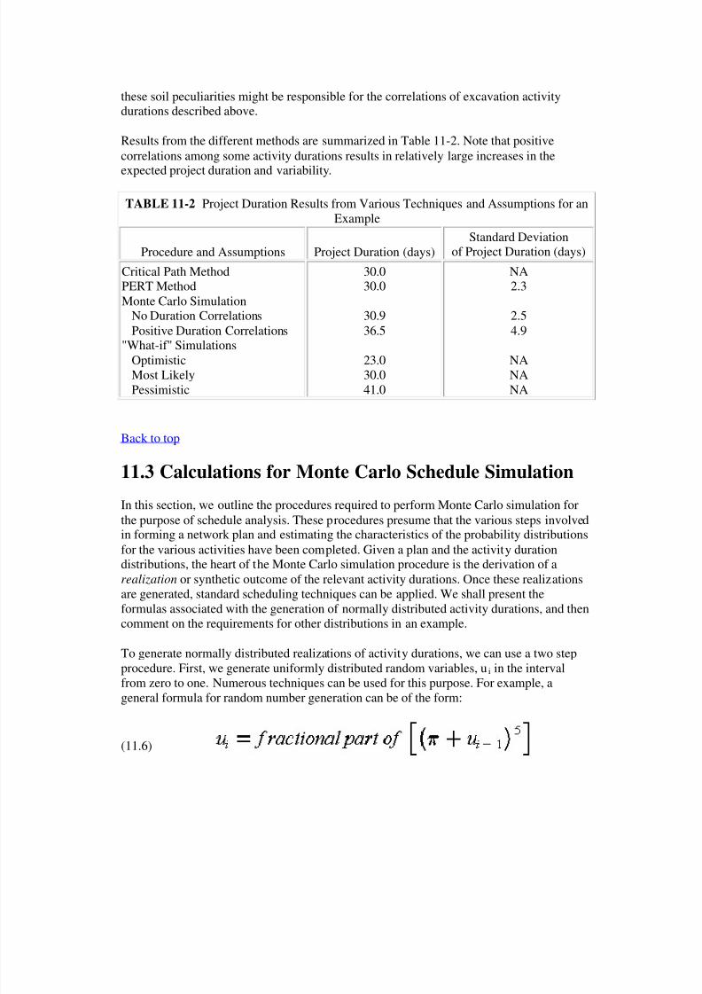
Results from the different methods are summarized in Table 11-2. Note that positivecorrelations among some activity durations results in relatively large increases in the

expected project duration and variability.

TABLE 11-2 Project Duration Results from Various Techniques and Assumptions for anExample

Procedure and Assumptions Project Duration (days)Standard Deviation

of Project Duration (days)

Critical Path MethodPERT MethodMonte Carlo Simulation

No Duration CorrelationsPositive Duration Correlations

"What-if" SimulationsOptimisticMost LikelyPessimistic

30.030.0

30.936.5

23.030.041.0

NA2.3

2.54.9

NANANA

Back to top

11.3 Calculations for Monte Carlo Schedule Simulation

In this section, we outline the procedures required to perform Monte Carlo simulation for

the purpose of schedule analysis. These procedures presume that the various steps involvedin forming a network plan and estimating the characteristics of the probability distributionsfor the various activities have been completed. Given a plan and the activity durationdistributions, the heart of the Monte Carlo simulation procedure is the derivation of arealization or synthetic outcome of the relevant activity durations. Once these realizationsare generated, standard scheduling techniques can be applied. We shall present theformulas associated with the generation of normally distributed activity durations, and thencomment on the requirements for other distributions in an example.

To generate normally distributed realizations of activity durations, we can use a two stepprocedure. First, we generate uniformly distributed random variables, ui in the intervalfrom zero to one. Numerous techniques can be used for this purpose. For example, a

general formula for random number generation can be of the form:

(11.6)



where = 3.14159265 and ui-1 was the previously generated random number or a pre-selected beginning or seed number. For example, a seed of u0 = 0.215 in Eq. (11.6) resultsin u1 = 0.0820, and by applying this value of u1, the result is u2 = 0.1029. This formula is aspecial case of the mixed congruential method of random number generation. WhileEquation (11.6) will result in a series of numbers that have the appearance and the

necessary statistical properties of true random numbers, we should note that these areactually "pseudo" random numbers since the sequence of numbers will repeat given a longenough time.

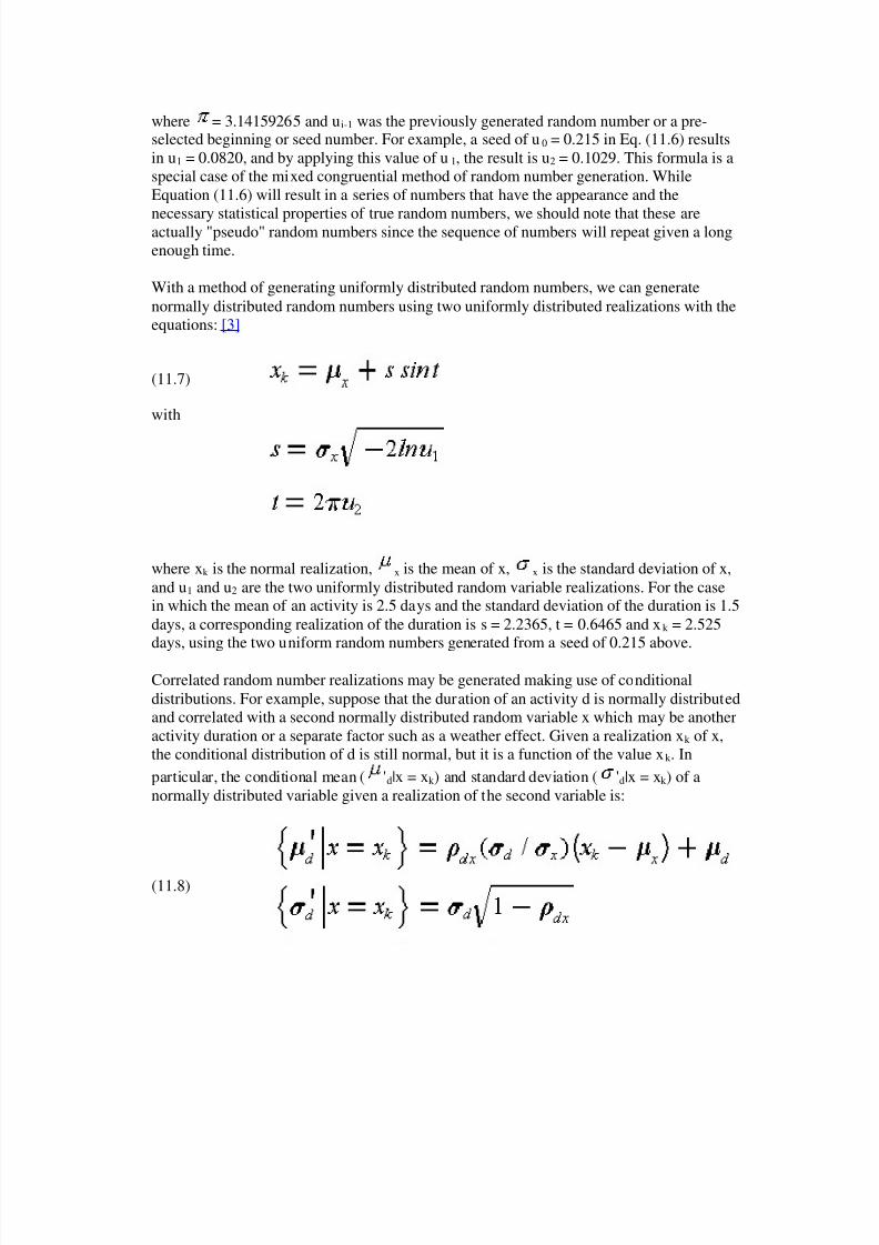
With a method of generating uniformly distributed random numbers, we can generatenormally distributed random numbers using two uniformly distributed realizations with theequations: [3]

(11.7)

with

where xk is the normal realization, x is the mean of x, x is the standard deviation of x,and u1 and u2 are the two uniformly distributed random variable realizations. For the casein which the mean of an activity is 2.5 days and the standard deviation of the duration is 1.5days, a corresponding realization of the duration is s = 2.2365, t = 0.6465 and xk = 2.525days, using the two uniform random numbers generated from a seed of 0.215 above.

Correlated random number realizations may be generated making use of conditionaldistributions. For example, suppose that the duration of an activity d is normally distributedand correlated with a second normally distributed random variable x which may be anotheractivity duration or a separate factor such as a weather effect. Given a realization xk of x,the conditional distribution of d is still normal, but it is a function of the value xk . In

particular, the conditional mean ( 'd|x = xk ) and standard deviation ( 'd|x = xk ) of anormally distributed variable given a realization of the second variable is:

(11.8)



where dx is the correlation coefficient between d and x. Once xk is known, theconditional mean and standard deviation can be calculated from Eq. (11.8) and then arealization of d obtained by applying Equation (11.7).

Correlation coefficients indicate the extent to which two random variables will tend to vary

together. Positive correlation coefficients indicate one random variable will tend to exceedits mean when the other random variable does the same. From a set of n historicalobservations of two random variables, x and y, the correlation coefficient can be estimatedas:

(11.9)

The value of xy can range from one to minus one, with values near one indicating apositive, near linear relationship between the two random variables.

It is also possible to develop formulas for the conditional distribution of a random variablecorrelated with numerous other variables; this is termed a multi-variate distribution. [4] Random number generations from other types of distributions are also possible. [5] Once aset of random variable distributions is obtained, then the process of applying a schedulingalgorithm is required as described in previous sections.

Example 11-2: A Three-Activity Project Example

Suppose that we wish to apply a Monte Carlo simulation procedure to a simple projectinvolving three activities in series. As a result, the critical path for the project includes allthree activities. We assume that the durations of the activities are normally distributed withthe following parameters:

Activity Mean (Days) Standard Deviation (Days)

ABC

2.55.62.4

1.52.42.0

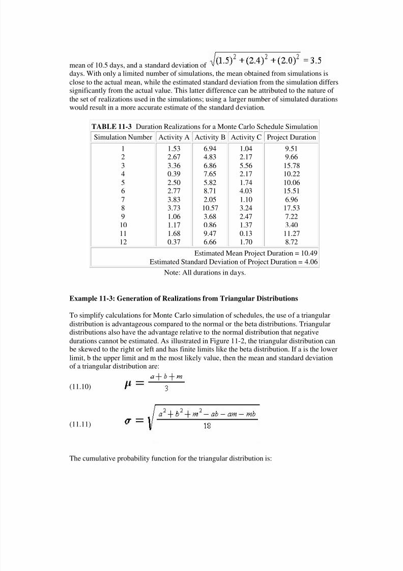
To simulate the schedule effects, we generate the duration realizations shown in Table 11-3and calculate the project duration for each set of three activity duration realizations.

For the twelve sets of realizations shown in the table, the mean and standard deviation of the project duration can be estimated to be 10.49 days and 4.06 days respectively. In thissimple case, we can also obtain an analytic solution for this duration, since it is only thesum of three independent normally distributed variables. The actual project duration has a



mean of 10.5 days, and a standard deviation of days. With only a limited number of simulations, the mean obtained from simulations isclose to the actual mean, while the estimated standard deviation from the simulation differssignificantly from the actual value. This latter difference can be attributed to the nature of

the set of realizations used in the simulations; using a larger number of simulated durationswould result in a more accurate estimate of the standard deviation.

TABLE 11-3 Duration Realizations for a Monte Carlo Schedule Simulation

Simulation Number Activity A Activity B Activity C Project Duration

123456

789101112

1.532.673.360.392.502.77

3.833.731.061.171.680.37

6.944.836.867.655.828.71

2.0510.573.680.869.476.66

1.042.175.562.171.744.03

1.103.242.471.370.131.70

9.519.66

15.7810.2210.0615.51

6.9617.537.223.40

11.278.72

Estimated Mean Project Duration = 10.49Estimated Standard Deviation of Project Duration = 4.06

Note: All durations in days.

Example 11-3: Generation of Realizations from Triangular Distributions

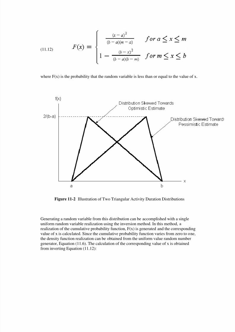
To simplify calculations for Monte Carlo simulation of schedules, the use of a triangulardistribution is advantageous compared to the normal or the beta distributions. Triangulardistributions also have the advantage relative to the normal distribution that negativedurations cannot be estimated. As illustrated in Figure 11-2, the triangular distribution canbe skewed to the right or left and has finite limits like the beta distribution. If a is the lowerlimit, b the upper limit and m the most likely value, then the mean and standard deviationof a triangular distribution are:

(11.10)

(11.11)

The cumulative probability function for the triangular distribution is:



(11.12)

where F(x) is the probability that the random variable is less than or equal to the value of x.

Figure 11-2 Illustration of Two Triangular Activity Duration Distributions

Generating a random variable from this distribution can be accomplished with a singleuniform random variable realization using the inversion method. In this method, arealization of the cumulative probability function, F(x) is generated and the corresponding

value of x is calculated. Since the cumulative probability function varies from zero to one,the density function realization can be obtained from the uniform value random numbergenerator, Equation (11.6). The calculation of the corresponding value of x is obtainedfrom inverting Equation (11.12):



(11.13)

For example, if a = 3.2, m = 4.5 and b = 6.0, then x = 4.8 and x = 2.7. With a uniform

realization of u = 0.215, then for (m-a)/(b-a) 0.215, x will lie between a and m and isfound to have a value of 4.1 from Equation (11.13).

Back to top

11.4 Crashing and Time/Cost Tradeoffs

The previous sections discussed the duration of activities as either fixed or randomnumbers with known characteristics. However, activity durations can often vary dependingupon the type and amount of resources that are applied. Assigning more workers to aparticular activity will normally result in a shorter duration. [6] Greater speed may result inhigher costs and lower quality, however. In this section, we shall consider the impacts of time, cost and quality tradeoffs in activity durations. In this process, we shall discuss theprocedure of project crashing as described below.

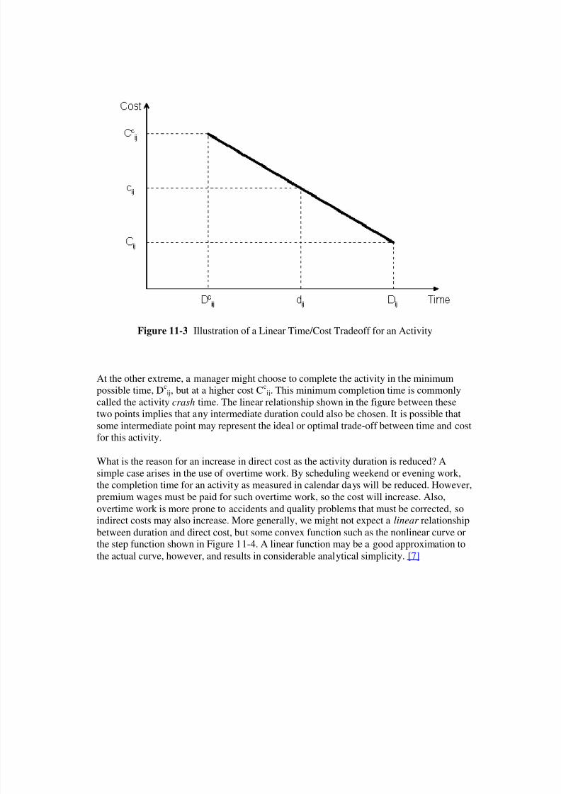
A simple representation of the possible relationship between the duration of an activity andits direct costs appears in Figure 11-3. Considering only this activity in isolation andwithout reference to the project completion deadline, a manager would undoubtedly choosea duration which implies minimum direct cost, represented by D

ijand C

ijin the figure.

Unfortunately, if each activity was scheduled for the duration that resulted in the minimumdirect cost in this way, the time to complete the entire project might be too long andsubstantial penalties associated with the late project start-up might be incurred. This is asmall example of sub-optimization, in which a small component of a project is optimized orimproved to the detriment of the entire project performance. Avoiding this problem of sub-optimization is a fundamental concern of project managers.



Figure 11-3 Illustration of a Linear Time/Cost Tradeoff for an Activity

At the other extreme, a manager might choose to complete the activity in the minimumpossible time, Dc

ij, but at a higher cost Ccij. This minimum completion time is commonly

called the activity crash time. The linear relationship shown in the figure between these

two points implies that any intermediate duration could also be chosen. It is possible thatsome intermediate point may represent the ideal or optimal trade-off between time and costfor this activity.

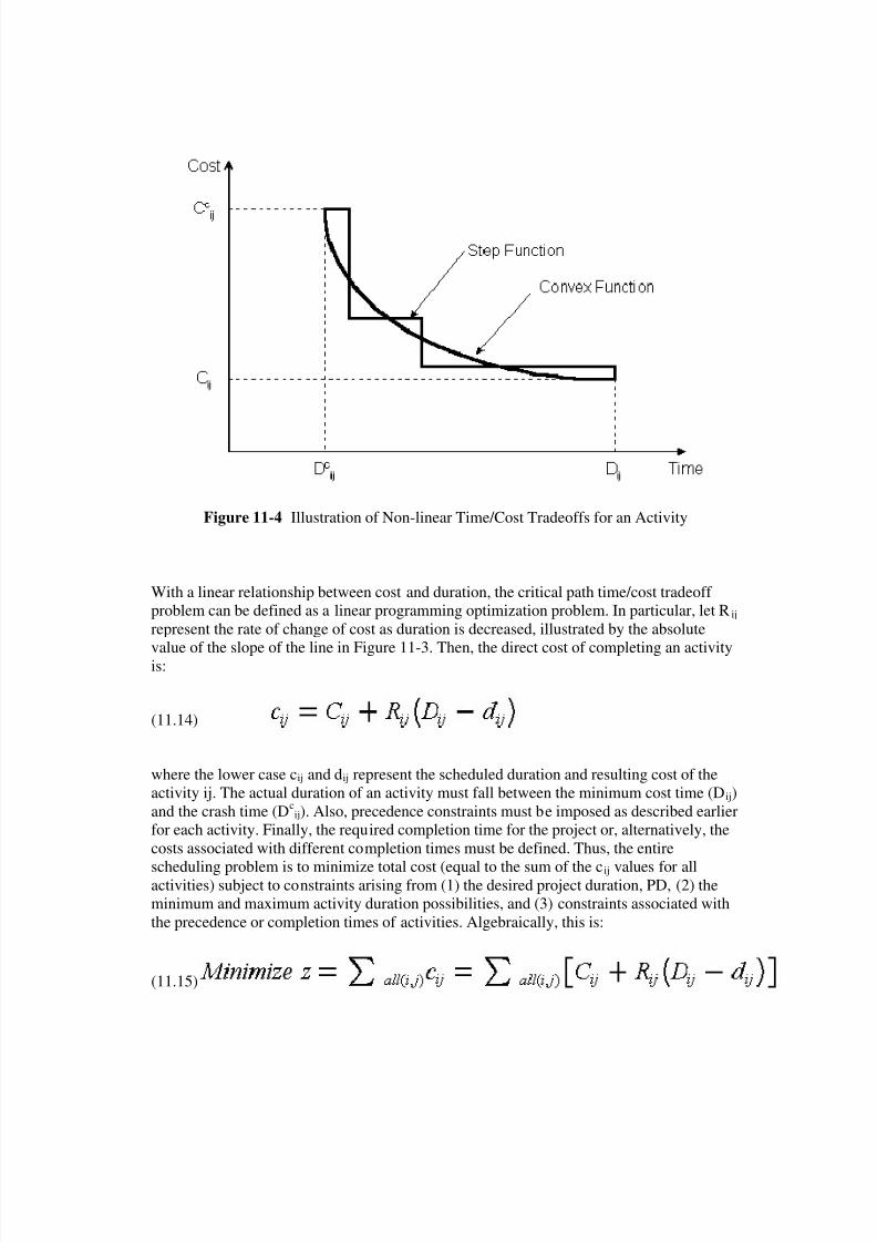
What is the reason for an increase in direct cost as the activity duration is reduced? Asimple case arises in the use of overtime work. By scheduling weekend or evening work,the completion time for an activity as measured in calendar days will be reduced. However,premium wages must be paid for such overtime work, so the cost will increase. Also,overtime work is more prone to accidents and quality problems that must be corrected, soindirect costs may also increase. More generally, we might not expect a linear relationshipbetween duration and direct cost, but some convex function such as the nonlinear curve orthe step function shown in Figure 11-4. A linear function may be a good approximation to

the actual curve, however, and results in considerable analytical simplicity. [7]



Figure 11-4 Illustration of Non-linear Time/Cost Tradeoffs for an Activity

With a linear relationship between cost and duration, the critical path time/cost tradeoff problem can be defined as a linear programming optimization problem. In particular, let Rij represent the rate of change of cost as duration is decreased, illustrated by the absolute

value of the slope of the line in Figure 11-3. Then, the direct cost of completing an activityis:

(11.14)

where the lower case cij and dij represent the scheduled duration and resulting cost of theactivity ij. The actual duration of an activity must fall between the minimum cost time (Dij)and the crash time (D

cij). Also, precedence constraints must be imposed as described earlier

for each activity. Finally, the required completion time for the project or, alternatively, thecosts associated with different completion times must be defined. Thus, the entire

scheduling problem is to minimize total cost (equal to the sum of the cij values for allactivities) subject to constraints arising from (1) the desired project duration, PD, (2) theminimum and maximum activity duration possibilities, and (3) constraints associated withthe precedence or completion times of activities. Algebraically, this is:

(11.15)



subject to the constraints:

where the notation is defined above and the decision variables are the activity durations dij and event times x(k). The appropriate schedules for different project durations can be foundby repeatedly solving this problem for different project durations PD. The entire problemcan be solved by linear programming or more efficient algorithms which take advantage of

the special network form of the problem constraints.

One solution to the time-cost tradeoff problem is of particular interest and deservesmention here. The minimum time to complete a project is called the project-crash time.This minimum completion time can be found by applying critical path scheduling with allactivity durations set to their minimum values (Dc

ij). This minimum completion time forthe project can then be used in the time-cost scheduling problem described above todetermine the minimum project-crash cost . Note that the project crash cost is not found bysetting each activity to its crash duration and summing up the resulting costs; this solutionis called the all-crash cost . Since there are some activities not on the critical path that canbe assigned longer duration without delaying the project, it is advantageous to change theall-crash schedule and thereby reduce costs.

Heuristic approaches are also possible to the time/cost tradeoff problem. In particular, asimple approach is to first apply critical path scheduling with all activity durations assumedto be at minimum cost (Dij). Next, the planner can examine activities on the critical pathand reduce the scheduled duration of activities which have the lowest resulting increase incosts. In essence, the planner develops a list of activities on the critical path ranked inaccordance with the unit change in cost for a reduction in the activity duration. Theheuristic solution proceeds by shortening activities in the order of their lowest impact oncosts. As the duration of activities on the shortest path are shortened, the project duration isalso reduced. Eventually, another path becomes critical, and a new list of activities on thecritical path must be prepared. By manual or automatic adjustments of this kind, good but

not necessarily optimal schedules can be identified. Optimal or best schedules can only beassured by examining changes in combinations of activities as well as changes to singleactivities. However, by alternating between adjustments in particular activity durations(and their costs) and a critical path scheduling procedure, a planner can fairly rapidlydevise a shorter schedule to meet a particular project deadline or, in the worst case, findthat the deadline is impossible of accomplishment.



This type of heuristic approach to time-cost tradeoffs is essential when the time-costtradeoffs for each activity are not known in advance or in the case of resource constraintson the project. In these cases, heuristic explorations may be useful to determine if greatereffort should be spent on estimating time-cost tradeoffs or if additional resources should beretained for the project. In many cases, the basic time/cost tradeoff might not be a smooth

curve as shown in Figure 11-4, but only a series of particular resource and schedulecombinations which produce particular durations. For example, a planner might have theoption of assigning either one or two crews to a particular activity; in this case, there areonly two possible durations of interest.

Example 11-4: Time/Cost Trade-offs

The construction of a permanent transitway on an expressway median illustrates thepossibilities for time/cost trade-offs in construction work. [8] One section of 10 miles of transitway was built in 1985 and 1986 to replace an existing contra-flow lane system (inwhich one lane in the expressway was reversed each day to provide additional capacity inthe peak flow direction). Three engineers' estimates for work time were prepared:

975 calendar day, based on 750 working days at 5 days/week and 8 hours/day of work plus 30 days for bad weather, weekends and holidays.

702 calendar days, based on 540 working days at 6 days/week and 10 hours/day of work.

360 calendar days, based on 7 days/week and 24 hours/day of work.

The savings from early completion due to operating savings in the contra-flow lane andcontract administration costs were estimated to be $5,000 per day.

In accepting bids for this construction work, the owner required both a dollar amount and acompletion date. The bidder's completion date was required to fall between 360 and 540

days. In evaluating contract bids, a $5,000 credit was allowed for each day less than 540days that a bidder specified for completion. In the end, the successful bidder completed theproject in 270 days, receiving a bonus of 5,000*(540-270) = $450,000 in the $8,200,000contract. However, the contractor experienced fifteen to thirty percent higher costs tomaintain the continuous work schedule.

Example 11-5: Time cost trade-offs and project crashing

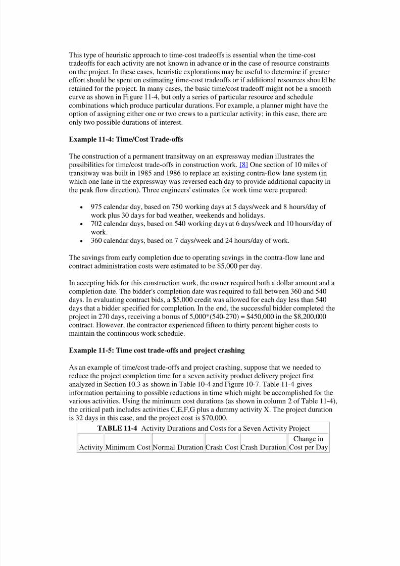
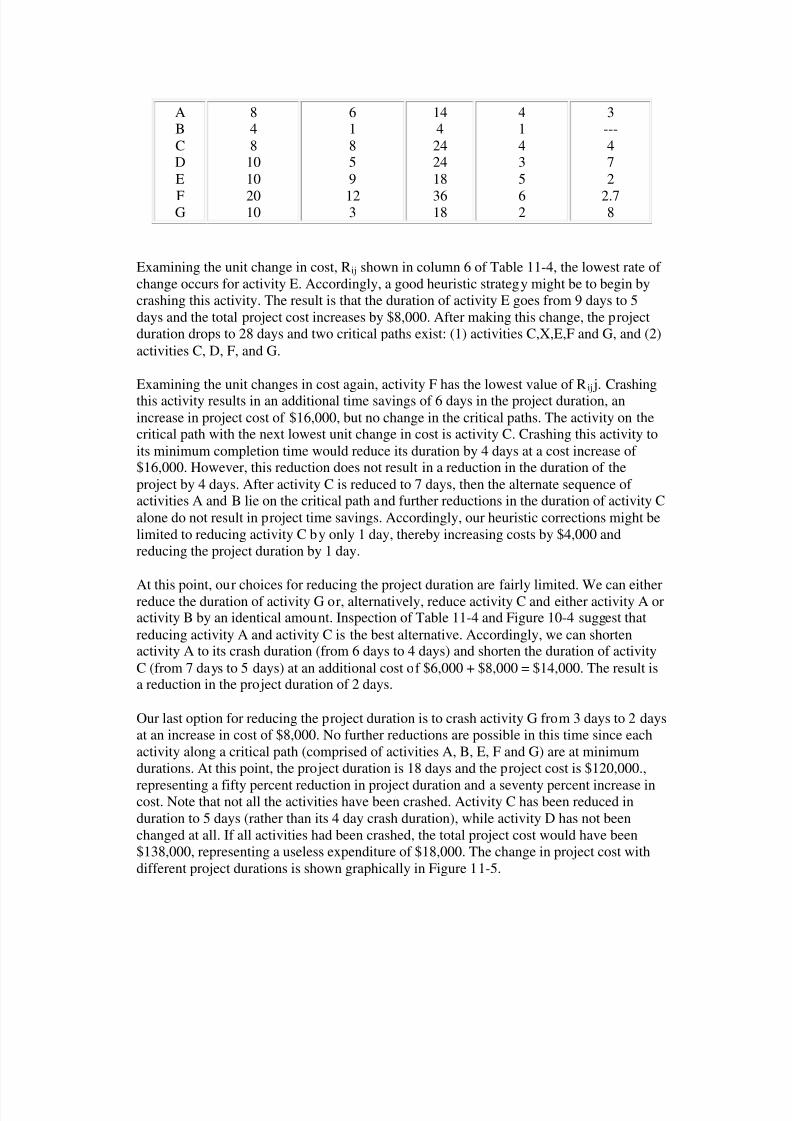
As an example of time/cost trade-offs and project crashing, suppose that we needed toreduce the project completion time for a seven activity product delivery project firstanalyzed in Section 10.3 as shown in Table 10-4 and Figure 10-7. Table 11-4 givesinformation pertaining to possible reductions in time which might be accomplished for thevarious activities. Using the minimum cost durations (as shown in column 2 of Table 11-4),the critical path includes activities C,E,F,G plus a dummy activity X. The project durationis 32 days in this case, and the project cost is $70,000.

TABLE 11-4 Activity Durations and Costs for a Seven Activity Project

Activity Minimum Cost Normal Duration Crash Cost Crash DurationChange in

Cost per Day



ABCDE

FG

848

1010

2010

61859

123

144242418

3618

41435

62

3---472

2.78

Examining the unit change in cost, Rij shown in column 6 of Table 11-4, the lowest rate of change occurs for activity E. Accordingly, a good heuristic strategy might be to begin bycrashing this activity. The result is that the duration of activity E goes from 9 days to 5days and the total project cost increases by $8,000. After making this change, the projectduration drops to 28 days and two critical paths exist: (1) activities C,X,E,F and G, and (2)activities C, D, F, and G.

Examining the unit changes in cost again, activity F has the lowest value of Rij j. Crashingthis activity results in an additional time savings of 6 days in the project duration, anincrease in project cost of $16,000, but no change in the critical paths. The activity on thecritical path with the next lowest unit change in cost is activity C. Crashing this activity toits minimum completion time would reduce its duration by 4 days at a cost increase of $16,000. However, this reduction does not result in a reduction in the duration of theproject by 4 days. After activity C is reduced to 7 days, then the alternate sequence of activities A and B lie on the critical path and further reductions in the duration of activity Calone do not result in project time savings. Accordingly, our heuristic corrections might belimited to reducing activity C by only 1 day, thereby increasing costs by $4,000 andreducing the project duration by 1 day.

At this point, our choices for reducing the project duration are fairly limited. We can eitherreduce the duration of activity G or, alternatively, reduce activity C and either activity A oractivity B by an identical amount. Inspection of Table 11-4 and Figure 10-4 suggest thatreducing activity A and activity C is the best alternative. Accordingly, we can shortenactivity A to its crash duration (from 6 days to 4 days) and shorten the duration of activityC (from 7 days to 5 days) at an additional cost of $6,000 + $8,000 = $14,000. The result isa reduction in the project duration of 2 days.

Our last option for reducing the project duration is to crash activity G from 3 days to 2 daysat an increase in cost of $8,000. No further reductions are possible in this time since eachactivity along a critical path (comprised of activities A, B, E, F and G) are at minimumdurations. At this point, the project duration is 18 days and the project cost is $120,000.,

representing a fifty percent reduction in project duration and a seventy percent increase incost. Note that not all the activities have been crashed. Activity C has been reduced induration to 5 days (rather than its 4 day crash duration), while activity D has not beenchanged at all. If all activities had been crashed, the total project cost would have been$138,000, representing a useless expenditure of $18,000. The change in project cost withdifferent project durations is shown graphically in Figure 11-5.



Figure 11-5 Project Cost Versus Time for a Seven Activity Project

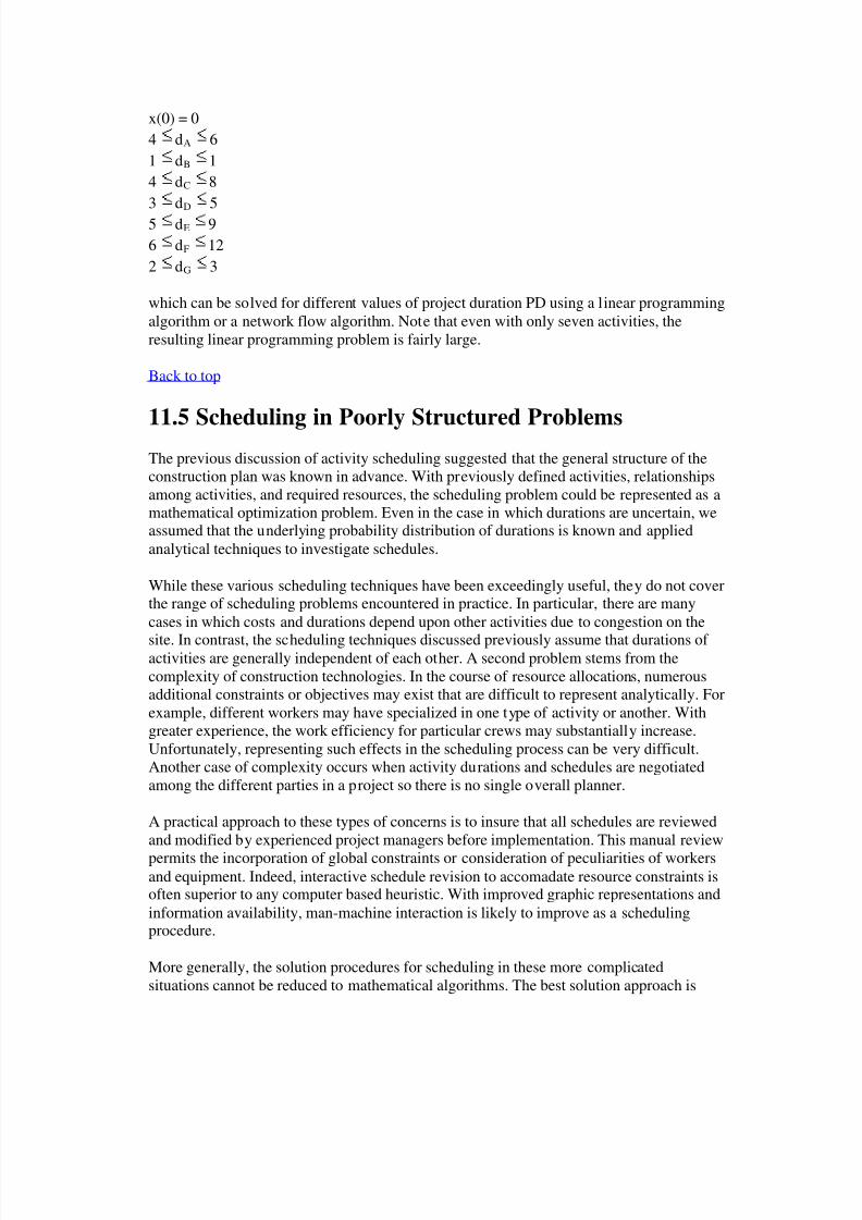
Example 11-8: Mathematical Formulation of Time-Cost Trade-offs

The same results obtained in the previous example could be obtained using a formal

optimization program and the data appearing in Tables 10-4 and 11-4. In this case, theheuristic approach used above has obtained the optimal solution at each stage. Using Eq.(11.15), the linear programming problem formulation would be:

Minimize z

= [8+3(6-dA)] + [4] + [8+4(8-dC)] + [10+7(5-dD)]

+ [10+2(9-dE)] + [20+2.7(9-dF)] + [10+2(3-dG)]

subject to the constraints

x(6) = PD x(0) + dA x(2)

x(0) + dC x(1)

x(1) x(3)

x(2) + dB x(4)

x(1) + dD x(4)

x(2) + dE x(4)

x(4) + dF x(5)

x(5) + dG x(6)



x(0) = 0

4 dA 6

1 dB 1

4 dC 8

3 dD 5

5 dE 9

6 dF 12

2 dG 3

which can be solved for different values of project duration PD using a linear programmingalgorithm or a network flow algorithm. Note that even with only seven activities, theresulting linear programming problem is fairly large.

Back to top

11.5 Scheduling in Poorly Structured ProblemsThe previous discussion of activity scheduling suggested that the general structure of theconstruction plan was known in advance. With previously defined activities, relationshipsamong activities, and required resources, the scheduling problem could be represented as amathematical optimization problem. Even in the case in which durations are uncertain, weassumed that the underlying probability distribution of durations is known and appliedanalytical techniques to investigate schedules.

While these various scheduling techniques have been exceedingly useful, they do not coverthe range of scheduling problems encountered in practice. In particular, there are manycases in which costs and durations depend upon other activities due to congestion on the

site. In contrast, the scheduling techniques discussed previously assume that durations of activities are generally independent of each other. A second problem stems from thecomplexity of construction technologies. In the course of resource allocations, numerousadditional constraints or objectives may exist that are difficult to represent analytically. Forexample, different workers may have specialized in one type of activity or another. Withgreater experience, the work efficiency for particular crews may substantially increase.Unfortunately, representing such effects in the scheduling process can be very difficult.Another case of complexity occurs when activity durations and schedules are negotiatedamong the different parties in a project so there is no single overall planner.

A practical approach to these types of concerns is to insure that all schedules are reviewedand modified by experienced project managers before implementation. This manual review

permits the incorporation of global constraints or consideration of peculiarities of workersand equipment. Indeed, interactive schedule revision to accomadate resource constraints isoften superior to any computer based heuristic. With improved graphic representations andinformation availability, man-machine interaction is likely to improve as a schedulingprocedure.

More generally, the solution procedures for scheduling in these more complicatedsituations cannot be reduced to mathematical algorithms. The best solution approach is



likely to be a "generate-and-test" cycle for alternative plans and schedules. In this process,a possible schedule is hypothesized or generated. This schedule is tested for feasibility withrespect to relevant constraints (such as available resources or time horizons) anddesireability with respect to different objectives. Ideally, the process of evaluating analternative will suggest directions for improvements or identify particular trouble spots.

These results are then used in the generation of a new test alternative. This processcontinues until a satisfactory plan is obtained.

Two important problems must be borne in mind in applying a "generate-and-test" strategy.First, the number of possible plans and schedules is enormous, so considerable insight tothe problem must be used in generating reasonable alternatives. Secondly, evaluatingalternatives also may involve considerable effort and judgment. As a result, the number of actual cycles of alternative testing that can be accomadated is limited. One hope forcomputer technology in this regard is that the burdensome calculations associated with thistype of planning may be assumed by the computer, thereby reducing the cost and requiredtime for the planning effort. Some mechanisms along these lines are described in Chapter15.

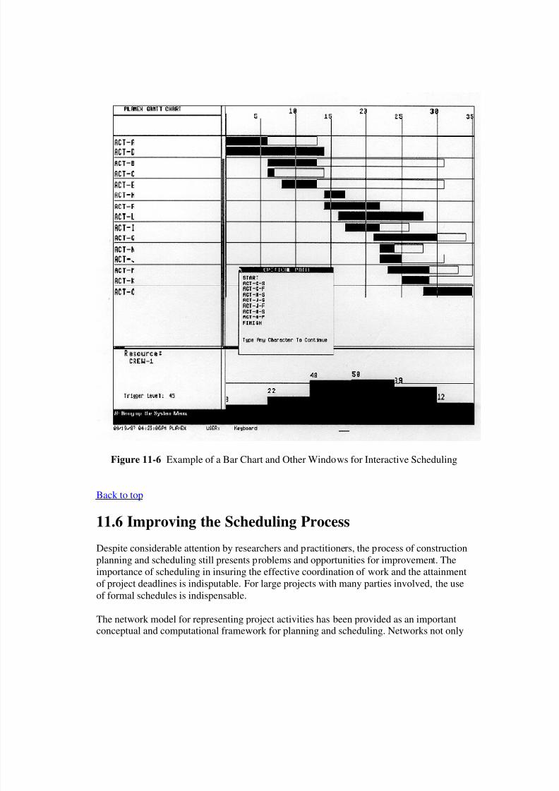
Example 11-9: Man-machine Interactive Scheduling

An interactive system for scheduling with resource constraints might have the followingcharacteristics: [9]

graphic displays of bar charts, resource use over time, activity networks and othergraphic images available in different windows of a screen simultaneously,

descriptions of particular activities including allocated resources and chosentechnologies available in windows as desired by a user,

a three dimensional animation of the construction process that can be stopped toshow the progress of construction on the facility at any time,

easy-to-use methods for changing start times and allocated resources, and utilities to run relevant scheduling algorithms such as the critical path method at

any time.

Figure 11-6 shows an example of a screen for this system. In Figure 11-6, a bar chartappears in one window, a description of an activity in another window, and a graph of theuse of a particular resource over time appears in a third window. These different"windows" appear as sections on a computer screen displaying different types of information. With these capabilities, a project manager can call up different pictures of theconstruction plan and make changes to accomadate objectives or constraints that are notformally represented. With rapid response to such changes, the effects can be immediatelyevaluated.



Figure 11-6 Example of a Bar Chart and Other Windows for Interactive Scheduling

Back to top

11.6 Improving the Scheduling Process

Despite considerable attention by researchers and practitioners, the process of constructionplanning and scheduling still presents problems and opportunities for improvement. Theimportance of scheduling in insuring the effective coordination of work and the attainmentof project deadlines is indisputable. For large projects with many parties involved, the useof formal schedules is indispensable.

The network model for representing project activities has been provided as an importantconceptual and computational framework for planning and scheduling. Networks not only



communicate the basic precedence relationships between activities, they also form the basisfor most scheduling computations.

As a practical matter, most project scheduling is performed with the critical pathscheduling method, supplemented by heuristic procedures used in project crash analysis or

resource constrained scheduling. Many commercial software programs are available toperform these tasks. Probabilistic scheduling or the use of optimization software to performtime/cost trade-offs is rather more infrequently applied, but there are software programsavailable to perform these tasks if desired.

Rather than concentrating upon more elaborate solution algorithms, the most importantinnovations in construction scheduling are likely to appear in the areas of data storage, easeof use, data representation, communication and diagnostic or interpretation aids.Integration of scheduling information with accounting and design information through themeans of database systems is one beneficial innovation; many scheduling systems do notprovide such integration of information. The techniques discussed in Chapter 14 areparticularly useful in this regard.

With regard to ease of use, the introduction of interactive scheduling systems, graphicaloutput devices and automated data acquisition should produce a very different environmentthan has existed. In the past, scheduling was performed as a batch operation with outputcontained in lengthy tables of numbers. Updating of work progress and revising activityduration was a time consuming manual task. It is no surprise that managers viewedscheduling as extremely burdensome in this environment. The lower costs associated withcomputer systems as well as improved software make "user friendly" environments a realpossibility for field operations on large projects.

Finally, information representation is an area which can result in substantial improvements.While the network model of project activities is an extremely useful device to represent a

project, many aspects of project plans and activity inter-relationships cannot or have notbeen represented in network models. For example, the similarity of processes amongdifferent activities is usually unrecorded in the formal project representation. As a result,updating a project network in response to new information about a process such as concretepours can be tedious. What is needed is a much more flexible and complete representationof project information. Some avenues for change along these lines are discussed in Chapter15.

Back to top

11.7 References

1. Bratley, Paul, Bennett L. Fox and Linus E. Schrage, A Guide to Simulation,Springer-Verlag, 1973.

2. Elmaghraby, S.E., Activity Networks: Project Planning and Control by Network

Models, John Wiley, New York, 1977.3. Jackson, M.J., Computers in Construction Planning and Control, Allen & Unwin,

London, 1986.



4. Moder, J., C. Phillips and E. Davis, Project Management with CPM, PERT and Precedence Diagramming, Third Edition, Van Nostrand Reinhold Company, 1983.

Back to top

11.8 Problems

1. For the project defined in Problem 1 from Chapter 10, suppose that the early, mostlikely and late time schedules are desired. Assume that the activity durations areapproximately normally distributed with means as given in Table 10-16 and thefollowing standard deviations: A: 4; B: 10; C: 1; D: 15; E: 6; F: 12; G: 9; H: 2; I: 4;J: 5; K: 1; L: 12; M: 2; N: 1; O: 5. (a) Find the early, most likely and late timeschedules, and (b) estimate the probability that the project requires 25% more timethan the expected duration.

2. For the project defined in Problem 2 from Chapter 10, suppose that the early, mostlikely and late time schedules are desired. Assume that the activity durations areapproximately normally distributed with means as given in Table 10-17 and thefollowing standard deviations: A: 2, B: 2, C: 1, D: 0, E: 0, F: 2; G: 0, H: 0, I: 0, J: 3;K: 0, L: 3; M: 2; N: 1. (a) Find the early, most likely and late time schedules, and(b) estimate the probability that the project requires 25% more time than theexpected duration.

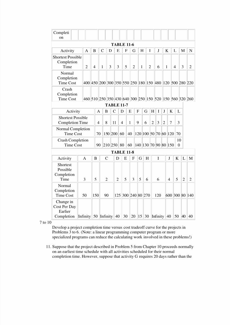
3 to 6The time-cost tradeoff data corresponding to each of the Problems 1 to 4 (inChapter 10), respectively are given in the table for the problem (Tables 11-5 to 11-8). Determine the all-crash and the project crash durations and cost based on theearly time schedule for the project. Also, suggest a combination of activity

durations which will lead to a project completion time equal to three days longerthan the project crash time but would result in the (approximately) maximumsavings.

TABLE 11-5

Activity A B C D E F G H I J K L M N O

ShortestPossibleCompletion Time 3 5 1 10 4 6 6 2 4 3 3 3 2 2 5

NormalCompleti

onTimeCost

150

250 80

400

220

300

260

120

200 180

220

500

100 120

500

Change inCost Per

DayEarlier 20 30

Infinity 15 20 25 10 35 20

Infinity 25 15 30

Infinity 10



Completion

TABLE 11-6

Activity A B C D E F G H I J K L M N

Shortest PossibleCompletion

Time 2 4 1 3 3 5 2 1 2 6 1 4 3 2

NormalCompletionTime Cost 400 450 200 300 350 550 250 180 150 480 120 500 280 220

CrashCompletionTime Cost 460 510 250 350 430 640 300 250 150 520 150 560 320 260

TABLE 11-7

Activity A B C D E F G H I J K L

Shortest PossibleCompletion Time 4 8 11 4 1 9 6 2 3 2 7 3

Normal CompletionTime Cost 70 150 200 60 40 120 100 50 70 60 120 70

Crash CompletionTime Cost 90 210 250 80 60 140 130 70 90 80 150

100

TABLE 11-8

Activity A B C D E F G H I J K L M

Shortest

PossibleCompletionTime 3 5 2 2 5 3 5 6 6 4 5 2 2

NormalCompletionTime Cost 50 150 90 125 300 240 80 270 120 600 300 80 140

Change inCost Per Day

EarlierCompletion Infinity 50 Infinity 40 30 20 15 30 Infinity 40 50 40 40

7 to 10

Develop a project completion time versus cost tradeoff curve for the projects inProblems 3 to 6. (Note: a linear programming computer program or morespecialized programs can reduce the calculating work involved in these problems!)

11. Suppose that the project described in Problem 5 from Chapter 10 proceeds normallyon an earliest time schedule with all activities scheduled for their normalcompletion time. However, suppose that activity G requires 20 days rather than the



expected 5. What might a project manager do to insure completion of the project bythe originally planned completion time?

12. For the project defined in Problem 1 from Chapter 10, suppose that a Monte Carlosimulation with ten repetitions is desired. Suppose further that the activity durations

have a triangular distribution with the following lower and upper bounds: A:4,8;B:4,9, C: 0.5,2; D: 10,20; E: 4,7; F: 7,10; G: 8, 12; H: 2,4; I: 4,7; J: 2,4; K: 2,6; L:10, 15; M: 2,9; N: 1,4; O: 4,11.(a) Calculate the value of m for each activity given the upper and lower bounds andthe expected duration shown in Table 10-16.(b) Generate a set of realizations for each activity and calculate the resulting projectduration.(c) Repeat part (b) five times and estimate the mean and standard deviation of theproject duration.

13. Suppose that two variables both have triangular distributions and are correlated.The resulting multi-variable probability density function has a triangular shape.

Develop the formula for the conditional distribution of one variable given thecorresponding realization of the other variable.

Back to top

11.9 Footnotes

1. See D. G. Malcolm, J.H. Rosenbloom, C.E. Clark, and W. Fazar, "Applications of aTechnique for R and D Program Evaluation," Operations Research, Vol. 7, No. 5, 1959,pp. 646-669. Back

2. See M.W. Sasieni, "A Note on PERT Times," Management Science, Vol. 32, No. 12, p1986, p. 1652-1653, and T.K. Littlefield and P.H. Randolph, "An Answer to Sasieni'sQuestion on Pert Times," Management Science, Vol. 33, No. 10, 1987, pp. 1357-1359. Fora general discussion of the Beta distribution, see N.L. Johnson and S. Kotz, Continuous

Univariate Distributions-2, John Wiley & Sons, 1970, Chapter 24. Back

3. See T. Au, R.M. Shane, and L.A. Hoel, Fundamentals of Systems Engineering -

Probabilistic Models, Addison-Wesley Publishing Company, 1972. Back

4. See N.L. Johnson and S. Kotz, Distributions in Statistics: Continuous Multivariate

Distributions, John Wiley & Sons, New York, 1973. Back

5. See, for example, P. Bratley, B. L. Fox and L.E. Schrage, A Guide to Simulation,Springer-Verlag, New York, 1983. Back

6. There are exceptions to this rule, though. More workers may also mean additionaltraining burdens and more problems of communication and management. Some activitiescannot be easily broken into tasks for numerous individuals; some aspects of computerprogramming provide notable examples. Indeed, software programming can be so perverse



that examples exist of additional workers resulting in slower project completion. See F.P.Brooks, jr. , The Mythical Man-Month, Addison Wesley, Reading, MA 1975. Back

7. For a discussion of solution procedures and analogies of the general function time/costtradeoff problem, see C. Hendrickson and B.N. Janson, "A Common Network Flow

Formulation for Several Civil Engineering Problems," Civil Engineering Systems, Vol. 1,No. 4, 1984, pp. 195-203. Back

8. This example was abstracted from work performed in Houston and reported in U.Officer, "Using Accelerated Contracts with Incentive Provisions for TransitwayConstruction in Houston," Paper Presented at the January 1986 Transportation ResearchBoard Annual Conference, Washington, D.C. Back

9. This description is based on an interactive scheduling system developed at CarnegieMellon University and described in C. Hendrickson, C. Zozaya-Gorostiza, D. Rehak, E.Baracco-Miller and P. Lim, "An Expert System for Construction Planning," ASCE Journal

of Computing, Vol. 1, No. 4, 1987, pp. 253-269. Back

Previous Chapter | Table of Contents | Next Chapter

const. mgmt. chp. 11 - advanced scheduling techniques

Documents