consistent linear-elastic transformations for image matching gary e. christensen department of...
TRANSCRIPT

Consistent Linear-Elastic Transformations for Image Matching
Gary E. Christensen
Department of Electrical & Computer EngineeringThe University of Iowa
This work was supported by NIH grant NS35368 and a grant from the Whitaker Foundation.

Introduction
• Uses of image registration• image segmentation/deformable atlas
• characterization of normal vs. abnormal shape/variation
• multi-modality fusion
• functional brain mapping/removing shape variation
• surgical planning and evaluation
• image guided surgery
• template constrained reconstruction
• Image registration methods• landmark, contour, surface, volume
Introduction
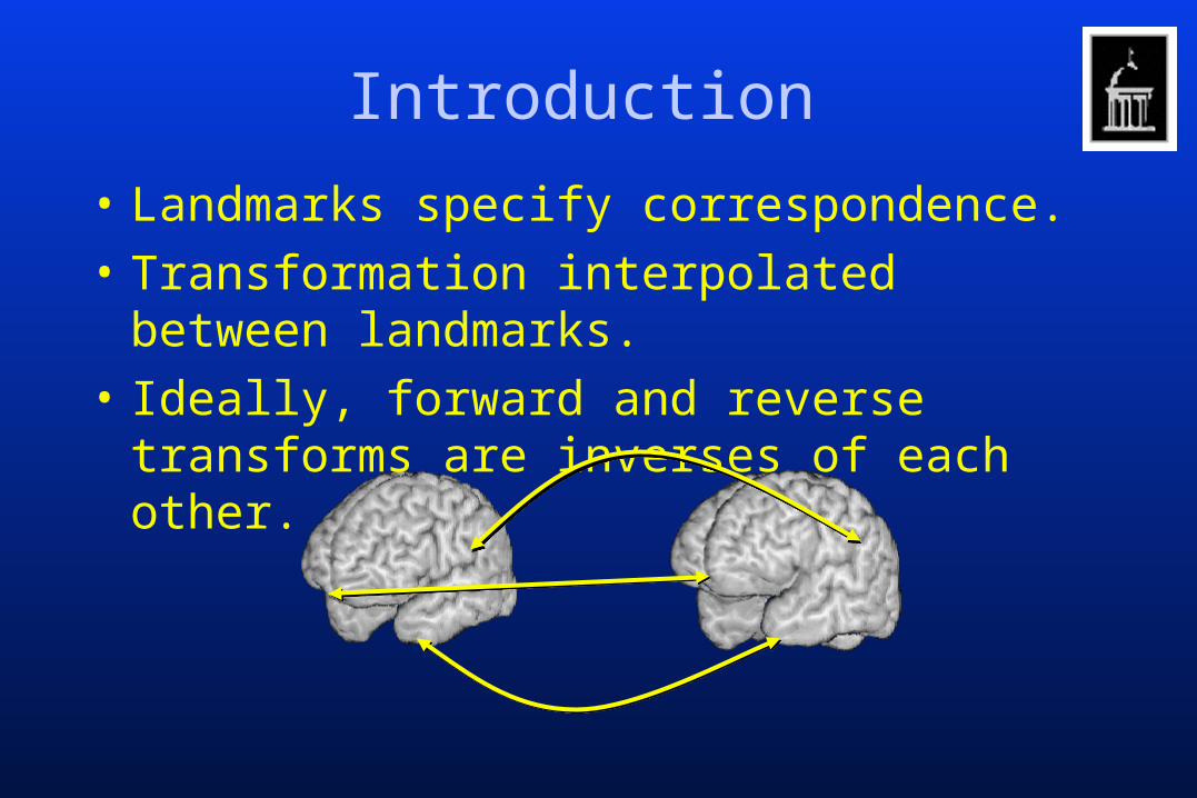
• Landmarks specify correspondence.
• Transformation interpolated between landmarks.
• Ideally, forward and reverse transforms are inverses of each other.

Introduction
• Limitations– Landmark
• manual identification, low-dimensional
– Contour• manual/semi-automatic, correspondence ambiguity
– Surface• semi-automatic/automatic, correspondence ambiguity
– Volume• automatic, correspondence ambiguity

Introduction• Woods et al., Automated Image Registration: II. Intersubject
Validation of Linear and Nonlinear Models, Journal of Computer Assisted Tomography, 22(1), 1998
• Pairwise consistency• Compute all pairwise registrations of a population using
the affine transformation model.
• Average the transformation from A to B with all the transformations from A to X to B.
• Replace the original transformation from A to B with average transformation. Repeat for all until convergence.

Introduction• Woods et al., Automated Image Registration: II. Intersubject
Validation of Linear and Nonlinear Models, Journal of Computer Assisted Tomography, 22(1), 1998
• Limitations• Does not apply for a population of two data sets.
• There is no guarantee that the generated set of consistent transformations are valid.
– ex. A poorly registered pair of images can adversely effect all of the pairwise transformations.

Introduction
• Consistent Transformation Estimation
– Jointly estimate the forward and reverse transformation between two image volumes
– Constrain the forward and reverse transformations to be inverses
– Constrain the transformations to preserve topology

Problem Statement
• Jointly estimate the transformations h and g such that h maps T to S and g maps S to T subject to the constraint that h = g-1

Transformation Properties
• From a biological standpoint, it is desirable that image registration algorithms produce transformations with the properties:
1. The transformation from image A to B is unique, i.e., the forward hab and reverse hba transformations are inverses of one another.
2. The transformations have the transitive property, i.e., hab(hbc(x)) = hac(x).
• Most image registration algorithms do not produce transformations with these properties.

Sources of Error:Inverse Consistency Error (EICC)
y=g(x)
x’ =h(y)
yx x’
Inverse Consistency Error = ||x-x’||where x’=h(g(x))

2D Landmark Experiment
• Compare thin-plate spline algorithms – Unidirectional vs. consistent registration*
*Consistent Landmark Registration: 2000 iterations, X harmonics = 50, Y harmonics = 50
Forward Reverse

Inverse Consistency Error(Cyclic Boundary Conditions)
5.0
0.00
A—B—A B—A—B A—B—A
TP
S
0.00
5.0
Con
sist
ent T
PS

Inverse Consistency Error(Cyclic Boundary Conditions)
5.0
0.00
A—B—A B—A—B A—B—A
TP
S
0.00
0.01
Con
sist
ent T
PS

Inverse Consistency Error(Cyclic Boundary Conditions)
5.0
0.00
0.00
0.01
A—B—A B—A—B
TP
SC
onsi
sten
t TP
S
Label Pixel Err.
A 5.0
B 0.008
B’ 0.27
C 3.9
D 0.008
D’ 0.33Label Pixel Err.
A 0.003
B 0.003
B’ 0.014
C 0.005
D 0.001
D’ 0.018
B
A
D
C
B
A
D
C

Notation
• Image volumes:– T(x) = Template S(x) = Target
• Coordinate system:
• Transformations:
)(~)()(~)(
)()()()(11 xwxxgxuxxh
xwxxgxuxxh
1:: ghgh
31,0x
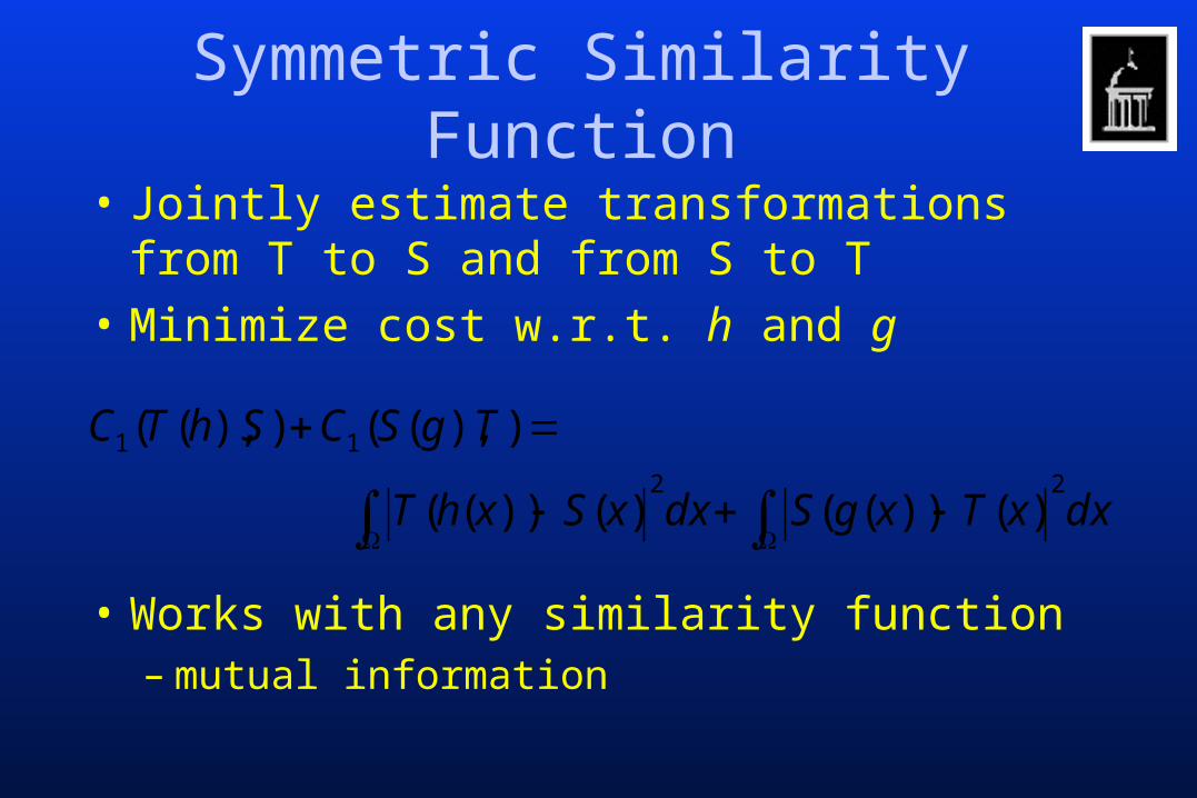
Symmetric Similarity Function
• Jointly estimate transformations from T to S and from S to T
• Minimize cost w.r.t. h and g
• Works with any similarity function– mutual information
dxxTxgSdxxSxhT
TgSCShTC22
11
)())(()())((
)),(()),((
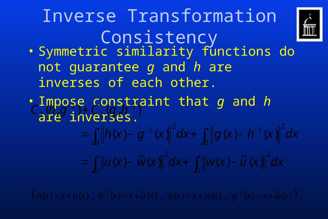
Inverse Transformation Consistency• Symmetric similarity functions do not guarantee g and h are inverses of each other.
• Impose constraint that g and h are inverses.
dxxuxwdxxwxu
dxxhxgdxxgxh
hgCghC
22
2121
12
12
)(~)()(~)(
)()()()(
),(),(
)(~)(),()(),(~)(),()( 11 xwxxgxwxxgxuxxhxuxxh

Diffeomorphic Transformations
h: • Onto
• Globally One-to-One
• Continuous– Compact sets are mapped to compact sets– Connected sets are mapped to connected sets– A composition of continuous transformations is
continuous
• Differentiable

Diffeomorphic Constraint
• The inverse consistency constraint only guarantees h and g are diffeomorphic transformations when
• To constrain h and g to be diffeomorphic, we use continuum mechanical models– linear elasticity– viscous fluid
0),(),( 12
12 hgCghC

Diffeomorphic Constraint
• Linear Elasticity
dxxLwdxxLuwCuC22
33 )()()()(
)(
)(
)(
)(
)(
)(
))(()()(
3
2
1
23
2
32
2
31
232
2
22
2
21
231
2
21
2
21
2
2
xu
xu
xu
xxxxx
xxxxx
xxxxx
xuxuxLu

1D Example• Complex exponentials are eigenfunctions of
constant coefficient difference equations
)(
1cos2
)()(2)()(
)(where)(
)(
ˆ
2
2ngDiscretizi
ˆ
2
2
xu
e
xuxuxuxLu
exux
xuxLu
i
xji
xj
i
i

Transformation Parameterization• Displacement fields (cyclic boundary conditions)
• coefficients– (3x1) complex-valued vectors– complex conjugate symmetry
N
k
N
j
N
iijk
N
k
N
j
N
i
xjijk
N
k
N
j
N
i
xjijk
ijk
ijk
exw
exu
2,
2,
2
1
0
1
0
1
0
,ˆ
1
0
1
0
1
0
,ˆ
where
)(
)(

Diffeomorphic Constraint
• Combining
• Gives
dxxLwdxxLuwCuC22
33 )()()()(
N
k
N
j
N
iijk
N
k
N
j
N
i
xjijk
N
k
N
j
N
i
xjijk
ijk
ijk
exw
exu
2,
2,
21
0
1
0
1
0
,ˆ
1
0
1
0
1
0
,ˆ
where)(
)(
1
0
1
0
1
0
2†2†333 )()(
N
k
N
j
N
iijkijkijkijkijkijk DDNwCuC

Diffeomorphic Constraint
• Linear Elasticity constraint
1
0
1
0
1
0
2†2†333 )()(
N
k
N
j
N
iijkijkijkijkijkijk DDNwCuC
kj
N
ikj
N
i
kiN
iki
N
i
jiN
iji
N
i
N
k
N
j
N
i
N
k
N
j
N
i
N
k
N
j
N
i
dd
dd
dd
d
d
d
223223
223113
222112
22233
22222
22211
coscos
coscos
coscos
cos1cos1cos12
cos1cos1cos12
cos1cos1cos12

Minimization Problem
• Find h and g that satisfy:
dxxLwxLu
dxxuxwxwxu
dxxTxgSxSxhTxgxhxgxh
22
22
22
)(),(
)()(
)(~)()(~)(
)())(()())((minarg)(ˆ),(ˆ
^ ^
and are Lagrange multipliers
)(~)(),()(),(~)(),()( 11 xwxxgxwxxgxuxxhxuxxh

Consistent Landmark• Consistent Landmark Cost Minimization
2 2
( ), ( )
2 21 1
2 2
1
ˆ ˆ( ), ( ) arg min ( ) ( )
( ) ( ) ( ) ( )
( ) ( )
h x g x
M
i i i i i i i ii
h x g x Lu x Lw x dx
h x g x g x h x dx
p u p q q w q p

Minimization Algorithm• Gradient descent is used to solve for new basis
coefficients at each iteration.
• Coarse to fine registration– Start algorithm with 0 and 1st harmonics.– Increase the number of harmonics by one after every
N iterations.
• The reverse basis coefficients are fixed while estimating the forward basis coefficients and visa versa.
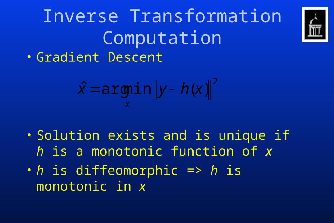
• Gradient Descent
• Solution exists and is unique if h is a monotonic function of x
• h is diffeomorphic => h is monotonic in x
Inverse Transformation Computation
2)(minargˆ xhyx
x

3D CT Inverse Consistency Experiment
• Use 3D CT data of infant heads
• Transform data volume A to B, and vice versa– Traditional linear-elasticity model – Consistent linear-elasticity model
• Combine the forward & reverse transformations
• Compare the composite transformation to Identity

3D CT Inverse Consistency Experiment
X-Dev. Y-Dev. Mag. Dev.
Error of composite mapping hab(hba(x)) using the linear elastic model without inverse consistency constraint.
Z-Dev.
Axial
Sagittal
Coronal
-0.94
1.2

3D CT Inverse Consistency Experiment
Error of composite mapping hab(hba(x)) with inverse consistency constraint using the linear elastic model.
X-Dev. Y-Dev. Mag. Dev.Z-Dev.
Axial
Sagittal
Coronal
-0.1
0.1

3D CT Inverse Consistency Experiment
Error of composite mapping hab(hba(x)) using the linear elastic model with & without inverse consistency constraint.
X-Dev. Y-Dev. Mag. Dev.Z-Dev.
-0.1
0.1
-0.94
1.2Without inverse
consistency
With inverse consistency
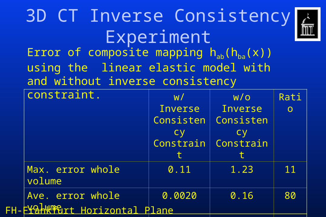
3D CT Inverse Consistency Experiment
w/ Inverse Consistency Constraint
w/o Inverse Consistency Constraint
Ratio
Max. error whole volume 0.11 1.23 11
Ave. error whole volume 0.0020 0.16 80
Max. error in head above FH 0.078 1.23 16
Ave. error in head above FH 0.0073 0.48 65
Error of composite mapping hab(hba(x)) using the linear elastic model with and without inverse consistency constraint.
FH-Frankfurt Horizontal Plane

Experiments• Eight experiments:
• MRI1: no constraints
• MRI2: linear elasticity
• MRI3: inverse consistency
• MRI4: lin. elast. and inv. consist.
• CT1: no constraints
• CT2: linear elasticity
• CT3: inverse consistency
• CT4: lin. elast. and inv. consist.

MRI4 Experiment
T S T(h) S(g) u1 u2 u3 w1 w2 w3
Christensen, IPMI’99

MRI4 Experiment
Christensen, IPMI’99

MRI4 Experiment
Christensen, IPMI’99

MRI4 Experiment
Christensen, IPMI’99

MRI4 Experiment
Christensen, IPMI’99

Transformation Measurements
Jacobian of h Jacobian of gExperiment min 1/max min 1/max C2(u,w) C2(w,u)
MRI1 0.257 0.275 0.100 0.261 28,300 29,500MRI2 0.521 0.459 0.371 0.653 10,505 10,460MRI3 0.315 0.290 0.226 0.464 478 479MRI4 0.607 0.490 0.410 0.640 186 186
~ ~
Christensen, IPMI’99

CT4 Experiment
T S T(h) S(g) u1 u2 u3 w1 w2 w3
Christensen, IPMI’99

CT4 Experiment
Christensen, IPMI’99

CT4 Experiment
Christensen, IPMI’99

CT4 Experiment
Christensen, IPMI’99

CT4 Experiment
Christensen, IPMI’99

Transformation Measurements
~ ~Jacobian of h Jacobian of g
Experiment min 1/max min 1/max C2(u,w) C2(w,u)
CT1 0.340 0.325 0.200 0.490 73,100 76,400CT2 0.552 0.490 0.421 0.678 28,700 28,300CT3 0.581 0.361 0.356 0.612 158 171CT4 0.720 0.501 0.488 0.725 167 189
Christensen, IPMI’99

Transformation Measurements
Jacobian of h Jacobian of gExperiment min 1/max min 1/max C2(u,w) C2(w,u)
MRI1 0.257 0.275 0.100 0.261 28,300 29,500MRI2 0.521 0.459 0.371 0.653 10,505 10,460MRI3 0.315 0.290 0.226 0.464 478 479MRI4 0.607 0.490 0.410 0.640 186 186CT1 0.340 0.325 0.200 0.490 73,100 76,400CT2 0.552 0.490 0.421 0.678 28,700 28,300CT3 0.581 0.361 0.356 0.612 158 171CT4 0.720 0.501 0.488 0.725 167 189
~ ~
Christensen, IPMI’99
Computational Costs
• Computational efficiency was achieved by using FFTs.
• Transforming one 643 voxel volume into another using 300 iterations takes approximately 25 minutes on a 180 MHz, R10000 processor.
• Computational time can be reduced by– reducing the number of iterations– using a more efficient optimization algorithm such as
conjugate gradient, etc.

Anatomical Variation
• Goal is to quantify the average shape & variability of anatomical populations.

Literature• Joshi et al., Gaussian Random Fields on Sub-manifolds for
Characterizing Brain Surfaces, XVth International Conference on Information Processing in Medical Imaging, eds. Duncan and Gindi, Poultney, VT, June,1997
• Miller et al., Statistical Methods in Computational Anatomy, Statistical Methods in Medical Research, vol. 6, 1997
• Woods et al., Automated Image Registration: II. Intersubject Validation of Linear and Nonlinear Models, Journal of Computer Assisted Tomography, 22(1), 1998

Synthesizing the Average
• Within a given population– Determine the “average” shape
– Determine the variability
i
i

Methods
1. Select one image volume from the population as the template
2. Estimate transformations by registering the template to all of the population images
3. Compute average and variance transformation from the estimated transformations
4. Compute synthesized average by applying the average transformation to the template image

Synthesizing the Average Shape
)1(T
)2(T
)3(T
)1(T
Template
2x
3x
y
)1,1(g
)2,1(g
)3,1(g
Population
)()1,1(1 ygx
)()2,1(2 ygx
)()3,1(3 ygx
1x

Synthesizing the Average Shape
)1(T
)2(T
)3(T
)1(T
Template
))(()( )1,1()1()1(xhTxT
1x
Population Average
2x
3x
y
1x)1,1(g
)2,1(g
)3,1(g
N
j
j ygN
ygx1
),1()1,1(1
)(1
)(
)()}({ )1,1()1,1(1
xhxginvy

Average and Variance Calculations
• Average:
• Variance:
M
ii xgxh
M 1
212 ))()((1
1
)()(
)(1
)(
1
1
1
xgTxT
xhM
xgM
ii

Results
Christensen et al., SPIE Medical Imaging 1999

Average and Original DataAvg. 1 2 3 4 5 6
128
146
163
Christensen et al., Synthesizing average 3D anatomical shapes using deformable templates,SPIE Medical Imaging 1999: Image Processing, ed. K.M. Hanson, SPIE vol. 3661.

ResultsAvg. 1 2 3

Skull Population
1 2 3 4 5

Synthesized Average Skulls
1 2 3 4 5
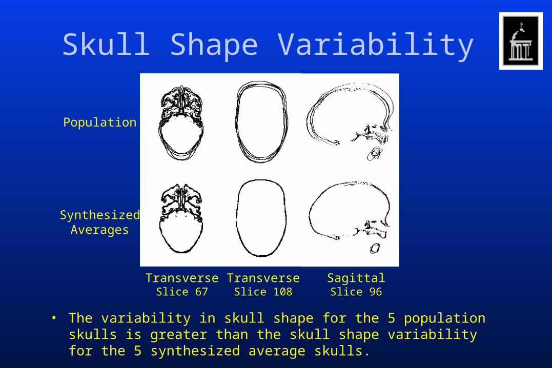
Skull Shape Variability
Population
SynthesizedAverages
• The variability in skull shape for the 5 population skulls is greater than the skull shape variability for the 5 synthesized average skulls.
TransverseSlice 67
TransverseSlice 108
SagittalSlice 96

Skull Shape Differences
Data Set
Average displacement of skull voxels (mm)
Variance of skull voxel displacements (mm2)
4.60 9.92
3.23 7.30
3.14 8.33
3.10 7.50
2.99 5.56
)1(T)2(T)3(T)4(T)5(T
2.742.63
2.572.72
2.222.79
2.562.64
2.592.70
)1(T
)2(T
)3(T
)4(T
)5(T
Average chamfer distance of skull voxels
(mm)
Variance of skull voxel chamfer distances (mm2)
2.51 7.08
1.42 4.80
1.39 4.96
1.26 4.38
1.36 4.071.11 2.44
0.952 2.24
1.08 2.51
1.02 2.42
1.04 2.58

20 Normal Adult Brains (Tns140hnnl)
Population Synthesized Averages

20 Normal Adult Brain Tracing (Tns140Avg)
Population Synthesized Averages

20 Normal Adult Brain Tracings (Tns140hnnl)
Brain1 Brain1Brain2
Brain1Brain2Brain3
Brain1 toBrain9
Brain1 toBrain20
Syn
thes
ized
Ave
rage
sP
opul
atio
n

20 Brain Contours
Population
SynthesizedAverages
Transverse Coronal Sagittal Sagittal Projection

Avg. Displacement Distance Projections

Var. Displacement Distance Projections

Brain Volume and Chamfer Distance Measures
AVG VAR Voxels AVG VAR Voxels001 3.32 0.92 3985 3.99 2.12 4156002 3.44 2.18 3960 5.40 9.00 3297003 3.35 0.86 3959 4.13 2.83 3730005 3.30 0.63 4000 4.89 2.83 4588006 3.54 1.65 3953 4.32 2.98 4171007 3.35 1.00 3984 4.37 3.89 4198008 3.66 4.03 3958 4.78 6.10 4227009 3.24 0.54 4002 4.08 2.14 4270011 3.30 0.70 3970 3.87 1.99 4053012 3.26 0.55 3967 4.10 2.18 3566013 3.23 0.50 3985 3.74 1.23 3998014 3.26 0.60 3979 3.71 1.28 3847015 3.26 0.59 3963 5.27 4.23 3256016 3.24 0.56 3992 3.69 1.69 3937017 3.27 0.54 4013 6.23 10.20 4768018 3.40 0.99 3957 3.98 2.04 3962019 3.24 0.55 3961 4.47 2.67 3478032 3.29 0.76 3972 3.71 1.28 3970104 3.33 0.58 3948 5.86 10.40 4665106 3.29 0.67 3960 3.99 2.49 3797AVG 3.33 0.97 3973 4.43 3.68 3997STD 0.10 0.81 18 0.72 2.83 403
Synthesized Averages Original Population

Bayesian Hypothesis Testing
• Empirically estimate a shape probability density – normal population p0(u)
– abnormal population p1(u)
• Use Bayesian hypothesis testing to determine if a test transformation is closer to hypothesis 0 or 1
p1(u)p0(u)
><H0
H1
)(~)()()( 00 pupxxu ii

Summary and Conclusions
• A new technique was presented for jointly estimating a consistent set of forward and reverse transformations.
• A new transformation model based on the Fourier series was presented and was used to simplify the discretized linear-elasticity constraint.
• The algorithm was efficiently implemented using FFTs.

Summary and Conclusions
• Unconstrained estimation leads to singular or near singular transformations.
• The linear-elastic constraint alone does not guarantee inverse consistency.
• The inverse consistency constraint alone does not guarantee nonsingular transformations during the iterative estimation procedure.
• The best results were generated using both the inverse consistency and linear-elastic constraints.

Summary and Conclusions
• A technique was presented for computing the average shape and variation of a population of data sets.
• Statistical shape models estimated in this fashion may be used to discriminate between normal and abnormal populations.

Acknowledgements
• This work was supported by NIH grant NS35368 and a grant from the Whitaker Foundation.
• We would also like to thank Richard Robb of the Mayo Clinic for his support in providing AnalyzeTM