consistent bond graph modelling of planar multibody systems · 174 t. bera & a. samantaray:...

ISSN 1 746-7233, England, UKWorld Journal of Modelling and Simulation

Vol. 7 (2011) No. 3, pp. 173-188

Consistent bond graph modelling of planar multibody systems

Tarun Kumar Bera , Arun Kumar Samantaray∗

Department of Mechanical Engineering, Indian Institute of Technology, Kharagpur 721302, India

(Received February 14 2010, Accepted February 1 2011)

Abstract. Modelling of mechanisms is not a trivial task because the goal is not only to obtain consistentkinematics but also to get proper dynamic loads. Therefore, a modular modelling approach is preferred forlarge and complex mechanisms. This paper discusses modular bond graph modelling of planar mechanicalsystems composed of rigid bodies, which are constrained together through a set of joints. Bond graph modelsof revolute joints with clearance and/or flexibility and mass distribution in prismatic or slider joints are de-veloped. Bond graph models obtained from hierarchical composition of subsystem models are then used tocalculate the dynamic loads. Two separate mechanisms are considered as illustrative examples and their bondgraph models are validated through numerical simulations.

Keywords: bond graph, multibody systems, rigid body mechanics, mechanisms

1 Introduction

Multibody systems consist of rigid and elastic bodies, various types of joint components[16], passive andactive coupling elements. Large transient dynamic forces are often setup in multibody systems, e.g. a tele-scopic rotary crane having a boom of elastic structure[20], and they are so often incorrectly neglected in thedesign stage due to improper modelling. These dynamic forces can be determined by simulation of a prop-erly developed model of the actual system or by experimentation. The first step in the dynamic analysis ofa mutibody system is the modelling of its components. In this article, we consider planar mechanisms withclosed kinematic loops. While simple mass lumping methods provide compact models, they often give in-correct dynamic forces due to incorrect representation of inertias and constraint forces. On the other hand,variational mass lumping method becomes too cumbersome when the mass distribution is time varying. Theobjective of this work is to develop hierarchically composable sub-models for elements of closed loop planarmechanisms which can be composed in different ways to assemble different forms of mechanisms while auto-matically taking care of the kinematic, dynamic and energetic consistency of the resultant model. By adoptingthe bond graph modelling formalism[3, 4, 9, 12, 18, 25], the concept of causality comes handy in segregating thesub-models, defining their composition architecture and ensuring the model consistency.

The equations of motion of a multibody system can be analyzed in different ways based on the principleused (Newton-Euler method, Principle of virtual work, Principle of virtual power etc.), coordinating systemused (Cartesian and Lagrangian coordinating systems), and the kinematic constraints of the system (Coordi-nate portioning method and augmented Lagrange formulation)[8]. The dynamic equations for the multibodysystems may be expressed by Jourdain’s principle and the Lagrange multiplier method together with Baum-garte’s stabilization[2, 15]. The number of equations increases when Lagrange multipliers are used. Moreover,when there is a little change in the configuration, the afore-mentioned process has to be repeated again, i.e., thederivation process is not in a modular algorithmic form. Modular approach [13] is essential when designing oranalyzing large/complex mechanisms. Linear graph theoretic approach[17] has been shown to be a good wayof modular representation of multibody system dynamics. Karnopp and Margolis [11] developed a systematic∗ Corresponding author. Tel.: +91 3222 282998/282999, fax: +91 322228227. E-mail address: [email protected].

Published by World Academic Press, World Academic Union

174 T. Bera & A. Samantaray: Consistent bond graph modelling of planar multibody systems

approach to modelling of planar mechanisms by using bond graphs[3, 4, 9, 12, 18, 25]. The bond graph formalismallows us to systematically organize large number of equations. Moreover, when the user modifies the model,the equations of motion are systematically derived from the revised model. Dymola [19] is an object orientedmodelling language, which provides a modular approach to model large interconnected systems. Various otherobject oriented bond graph software tools are also available commercially. Moreover, bond graph models areeasily portioned by breaking bonds and introducing interface ports. Partitioning of models and use of separatesimulation software tailored for specific subsystems have been explored recently in the context of multibodysystem simulation in reference[22].

To start with, we develop the bond graph model rigid planar links. Thereafter, we consider modelling offlexible joints and the impact forces at flexible joints with clearance. Then the model of a slider element withproper representation of contact forces is developed. Although simple kinematic relations are used to constructthis bond graph model, the model by itself takes care of Coriolis and centrifugal forces due to the inherentpower conservative properties of bond graph. This model shows the modularity of bond graph modelling indealing with complex mechanisms. Finally, we consider two case studies: a Rapson slide and a seven-bodymechanism[24]. The simulation results from these two models are compared with those obtained through othermeans and the results available in the literature.

Fig. 1. Schema for a three-port rigid link

2 Modelling of planar mechanisms

2.1 Model of rigid planar links

We use a body fixed frame x− y on a rigid link and relate the motions to the absolute frame of referencex − y through appropriate velocity transformation. The displacements of any point (ith point) on the rigidlink, as shown in Fig. 1, are expressed in terms of linear displacements (xG, yG) of the center of gravity in thex− y plane and angular position (θG) of the center of gravity about the z-axis as follows:[

xiyi

]=[xGyG

]+[

cos θG − sin θGsin θG − cos θG

] [xiyi

], (1)

where xi and yi define the position of a point in the body-fixed frame. Differentiating Eq. (1) with respect totime, and noting that and are constant in a rigid body, one obtains

xi = xG + µxi θG, (2)

yi = yG + µyi θG, (3)

where µxi = −(xi sin θG + yi cos θG) and µyi = xi cos θG − yi sin θG.

WJMS email for contribution: [email protected]

World Journal of Modelling and Simulation, Vol. 7 (2011) No. 3, pp. 173-188 175

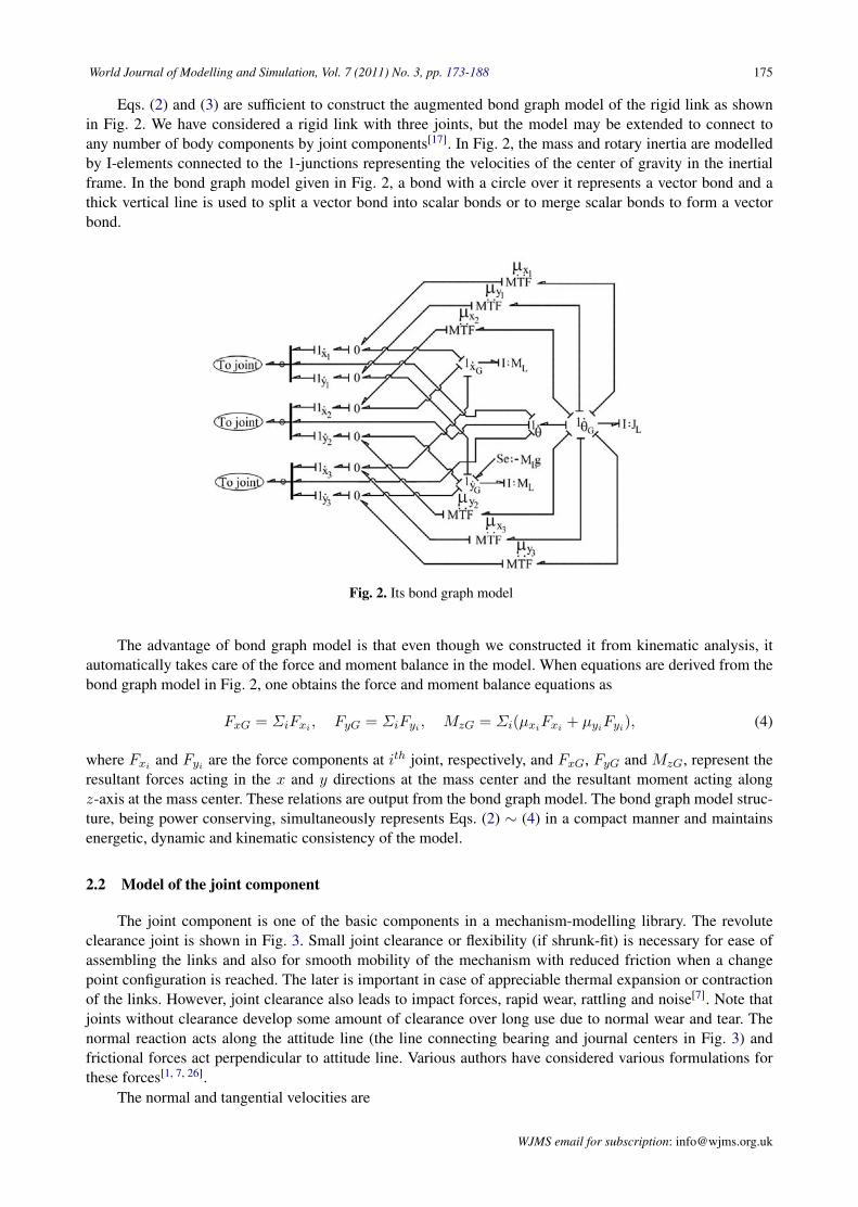
Eqs. (2) and (3) are sufficient to construct the augmented bond graph model of the rigid link as shownin Fig. 2. We have considered a rigid link with three joints, but the model may be extended to connect toany number of body components by joint components[17]. In Fig. 2, the mass and rotary inertia are modelledby I-elements connected to the 1-junctions representing the velocities of the center of gravity in the inertialframe. In the bond graph model given in Fig. 2, a bond with a circle over it represents a vector bond and athick vertical line is used to split a vector bond into scalar bonds or to merge scalar bonds to form a vectorbond.

Fig. 2. Its bond graph model

The advantage of bond graph model is that even though we constructed it from kinematic analysis, itautomatically takes care of the force and moment balance in the model. When equations are derived from thebond graph model in Fig. 2, one obtains the force and moment balance equations as

FxG = ΣiFxi , FyG = ΣiFyi , MzG = Σi(µxiFxi + µyiFyi), (4)

where Fxi and Fyi are the force components at ith joint, respectively, and FxG, FyG and MzG, represent theresultant forces acting in the x and y directions at the mass center and the resultant moment acting alongz-axis at the mass center. These relations are output from the bond graph model. The bond graph model struc-ture, being power conserving, simultaneously represents Eqs. (2) ∼ (4) in a compact manner and maintainsenergetic, dynamic and kinematic consistency of the model.

2.2 Model of the joint component

The joint component is one of the basic components in a mechanism-modelling library. The revoluteclearance joint is shown in Fig. 3. Small joint clearance or flexibility (if shrunk-fit) is necessary for ease ofassembling the links and also for smooth mobility of the mechanism with reduced friction when a changepoint configuration is reached. The later is important in case of appreciable thermal expansion or contractionof the links. However, joint clearance also leads to impact forces, rapid wear, rattling and noise[7]. Note thatjoints without clearance develop some amount of clearance over long use due to normal wear and tear. Thenormal reaction acts along the attitude line (the line connecting bearing and journal centers in Fig. 3) andfrictional forces act perpendicular to attitude line. Various authors have considered various formulations forthese forces[1, 7, 26].

The normal and tangential velocities are

WJMS email for subscription: [email protected]


Fig. 3. Bearing and journal of a clearance revolute joint Fig. 4. Bond graph model

Fig. 5. Its equivalent bond graph Fig. 6. Schema for rigid links and joint components

Vn =(x1 − x2) sinψ − (y1 − y2) cosψ, (5)

Vt =(x1 − x2) cosψ + (y1 − y2) sinψ + (θ1Rb − θ2Rj), (6)

where the variables are defined in Fig. 3. The penetration depth due to impact between the two componentsis given as δ = (BJ − c) where the radial clearance c = Rb − Rj . Note that δ is taken to be zero when(BJ − c) < 0. The normal contact force which is evaluated according to the relation given in [11] as

Fn = Kδα +[3Kδα(1− C2

e )4δ−

]δ for δ > 0, Fn = 0 otherwise. (7)

In Eq. (7) the first term denotes the elastic Hertzian contact force [11, 14] where the stiffness is calculatedas K = 4

√RbRj/(Rb +Rj)/3(η1 + η2), with ηi = (1 − ν2

i )/Ei are two material parameters[11], ν andE are the Poisson’s ratio and Young’s modulus, respectively, α is usually taken as 1.5 for contact betweenmetallic bodies, and Ce is the coefficient of restitution used to model impact. The second term in Eq. (7) isdue to internal damping of the materials which introduces strain rate dependent damping during impact withδ− being the initial impact velocity and δ is the relative penetration rate. In reference [14], Adams softwarehas been used to model impact forces where the instantaneous damping coefficient has been considered to bea cubic step function of the penetration.

The tangential force is calculated from the modified Coulomb’s friction law as follows[7]

Ft = −CfCdFnsgn(Vt), (8)

where Cf is coefficient of friction, Cd is dynamic correction coefficient (see [11] for details) and sgn(.) isthe signum function. Other forms of dry-friction formulations (e.g., stick-slip[10], honey-drop and Stribeckfriction model etc.) may be used here. The formulation given in reference [1] uses Poisson’s hypothesis forthe definition of the coefficient by first recognizing the correct mode of impact; i.e., sliding, sticking, andreverse sliding. If the clearance between the journal and the bearing is lubricated then fluid-film forces dictatethe normal and tangential forces. Bond graph model of journal bearings can be consulted in [21]. However,only dry-friction is considered in the models developed in this article.

The normal and tangential contact forces can be resolved into two components in x− y directions:



Fx = Fn sinψ + Ft cosψ and Fy = Fn cosψ + Ft sinψ. (9)

The moments acting at the bearing and the journal center due to tangential forces are, respectively,

Mb = FtRb and Mj = FtRj . (10)

The bond graph model of the revolute clearance joint is shown in Fig. 4 and its equivalent bond graph incompact form using vector bonds is shown in Fig. 5. The constitutive relation for the RC-field element (a fieldelement is connected to more than one bonds) is e = ϕRT (f ,

∫fdt, r) where r is a set of fixed parameters

(geometric and material properties), f = [x1, y1, θ1, x2, y2, θ2]T is the vector of generalized flow (veloc-ity) variables, e = [Fx1 , Fy1 ,Mz1 , Fx2 , Fy2 ,Mz2 ]

T is the vector of generalized effort variables and ϕRC(.)function models Eqs. (5) ∼ (10). Because the constitutive relation involves both the rate of deformation anddeformation to compute the effort (force and moment) variables, the physical phenomenon involved is a com-bination of dissipation and potential energy storage, which together are represented by a defined bond graphelement (RC-field). Note that the attitude angle ψ must be calculated using atan2(.) function such that thequadrant information in not lost during the process.

Three rigid links with joint components are shown in Fig. 6. One of these links is assumed to hold thecommon journal and is considered to be the reference link. The remaining links form parallel outer races.The clearances between two pairs (link 1 and link 2, and link 1 and link 3) of rigid links are shown in Fig. 7,where rcc is the radius of the clearance circle. The parameter δij (where i and j enumerate the links) is theinstantaneous distance between the centers of the bolt and the hole in the respective link ends. If no clearanceis provided between a pair of links, the corresponding value of rcc is zero. When δij > rcc, the interactionforce between a pair of links is modelled by Eqs. (7) and (8) and are transformed to inertial frame forces andmoments by Eqs. (9) and (10). The bond graph model of many links connected to the common reference linkis shown in Fig. 8 where the bold 1-junction is drawn using vector bond graph notation[12] and the dimensionof effort and flow variable vectors in each bond is three. This model is an extension of the model given inFig. 5. The generalized model given in Fig. 8 can be simplified if the joints do not have clearance. Such joints

Fig. 7. Its different clearances between two pair of rigidlinks

Fig. 8. Its bond graph model

without flexibility are referred to as kinematic joints. However, we will consider joint flexibility in our model.Note that if the joint stiffness is made large in a joint without clearance then the flexible joint behaves as anideal kinematic joint.

For the flexible joint without clearance, δ = BJ (from Fig. 3). Furthermore, since Rb = Rj , Hertziancontact theory is not applicable because the contact area is more than the characteristic radius of the bodies.The effective stiffness is then considered as K which has to be evaluated experimentally or numerically, e.g.,from a finite element model. The damping is proportional to effective stiffness. The proportionality constantsbetween stiffness and damping for various materials are tabulated in reference [6]. Note that without clearance,the stiffness and damping encountered in any radial direction is the same, i.e, the 2× 2 stiffness and dampingmatrices are symmetric and rotationally invariant.

The normal force is then given as

Fn = Kδ + λKδ, (11)



where λ is the material damping related proportionality constant[6]. The tangential force Ft is still given byEq. (8).

If dry-friction is neglected and viscous friction is considered (which can be modelled with relative angularvelocities) then Ft = 0. Consequently, the interaction forces in x−y reference frame between ith link and thereference link (link number 1) are given as(

FxFy

)=[K 00 K

]( ∫(xi − x1)dt∫(yi − y1)dt

)+[λK 00 λK

]((xi − x1)(yi − y1)

). (12)

Separation of the elastic and damping forces and their representation as separate fields (C-field and R-field)yield a simplified bond graph model for joints between several links as shown in Fig. 9. The viscous frictionbetween two links at the joint is modelled by separate R-elements at 0-junctions where relative angular ve-locities between the links and the reference link are calculated. Likewise, torsional stiffness and damping atthe joint may be modelled by 1-C-R structures connected to the 0-junction. If the joint is passive, i.e. actu-ated, then the motor model with appropriate causalities to apply a torque (effort) may be connected to that0-junction. The power directions in the bond graph model are set to calculate relative angular velocities at this0-junction. This also ensures that a motor would apply a forward torque on the driven link and the reversereactive torque on the driving link.

Fig. 9. Bond graph model of an ideal joint component with multiple shear and pin flexibility

When the values of joint stiffness and damping are large, there exists almost same generalized flow inall bonds connected to the joint element from the body components and the impedance coupling tends tobecome a plain coupling or kinematic joint. Decreasing the value of compliance element can increase the jointflexibility. If the values of damping and compliance parameters are taken to be zero then the connected bodycomponents are decoupled. This is how the type of the joint can be changed as per requirement.

2.3 Model of a slider component

The slider is one of the most difficult multibody components which give rise to nonlinear equations ofmotion. Incorrect modelling of slider components generates improper inertial forces. The schematic view of aplane slider is shown in Fig. 10. The main advantage of a bond graph model is that the radial and tangentialforces acting at different points of the model need not be calculated. Simulations supported by theoreticalbond graph model of the actual system can determine these dynamic forces.

The velocities of the end points Ec and EP of the plane slider are expressed as follows:

x1 = xcg + lcg θcg sin θcg, y1 = ycg − lcg θcg cos θcg,

x2 = xpg − lpg θpg sin θpg, y2 = ypg + lpg θpg cos θpg. (13)

The rate of change of contemporary length (l) between two points Ec and EP may be expressed as

l =(x1 − x2

l

)(x1 − x2) +

(y1 − y2

l

)(y1 − y2). (14)



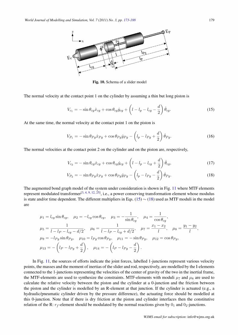
Fig. 10. Schema of a slider model

The normal velocity at the contact point 1 on the cylinder by assuming a thin but long piston is

Vc1 = − sin θcgxcg + cos θcgycg +(l − lp − lcg −

d

2

)θcg. (15)

At the same time, the normal velocity at the contact point 1 on the piston is

VP1 = − sin θPgxPg + cos θPgyPg −(lp − lPg +

d

2

)θPg. (16)

The normal velocities at the contact point 2 on the cylinder and on the piston are, respectively,

Vc2 =− sin θcgxcg + cos θcgycg +(l − lp − lcg +

d

2

)θcg, (17)

VP2 =− sin θPgxPg + cos θPgyPg −(lp − lPg −

d

2

)θPg. (18)

The augmented bond graph model of the system under consideration is shown in Fig. 11 where MTF elementsrepresent modulated transformer[3, 4, 9, 12, 25], i.e., a power conserving transformation element whose modulusis state and/or time dependent. The different multipliers in Eqs. (15) ∼ (18) used as MTF moduli in the modelare

µ1 = lcg sin θcg, µ2 = −lcg cos θcg, µ3 = − 1sin θcg

, µ4 =1

cos θcg,

µ5 =1

l − lP − lcg − d/2, µ6 =

1l − lP − lcg + d/2

, µ7 =x1 − x2

l, µ8 =

y1 − y2

l,

µ9 = −lPg sin θPg, µ10 = lPg cos θPg, µ11 = − sin θPg, µ12 = cos θPg,

µ13 = −(lP − lPg +

d

2

), µ14 = −

(lP − lPg −

d

2

).

In Fig. 11, the sources of efforts indicate the joint forces, labelled 1-junctions represent various velocitypoints, the masses and the moment of inertias of the slider and rod, respectively, are modelled by the I-elementsconnected to the 1-junctions representing the velocities of the center of gravity of the two in the inertial frame,the MTF-elements are used to synthesize the constraints. MTF-elements with moduli µ7 and µ8 are used tocalculate the relative velocity between the piston and the cylinder at a 0-junction and the friction betweenthe piston and the cylinder is modelled by an R-element at that junction. If the cylinder is actuated (e.g., ahydraulic/pneumatic cylinder driven by the pressure difference), the actuating force should be modelled atthis 0-junction. Note that if there is dry friction at the piston and cylinder interfaces then the constitutiverelation of the R: rf -element should be modulated by the normal reactions given by 01 and 02-junctions.



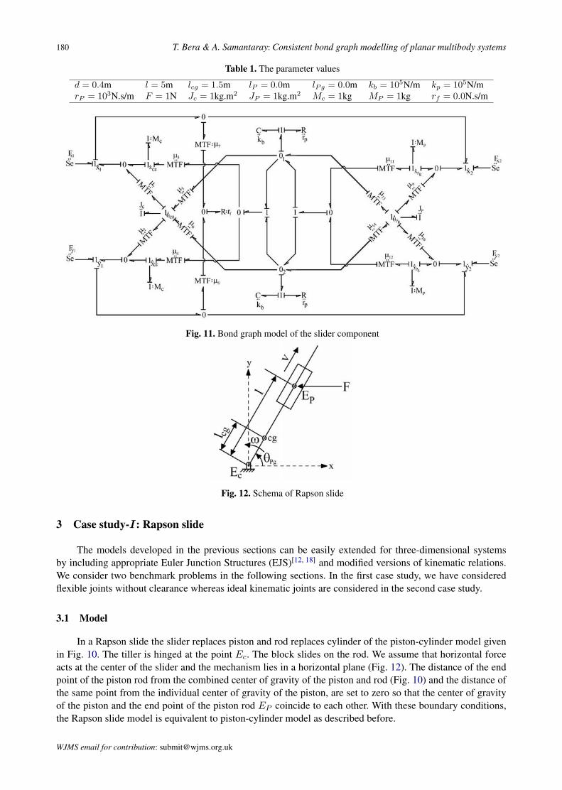
Table 1. The parameter values

d = 0.4m l = 5m lcg = 1.5m lP = 0.0m lPg = 0.0m kb = 105N/m kp = 105N/mrP = 103N.s/m F = 1N Jc = 1kg.m2 JP = 1kg.m2 Mc = 1kg MP = 1kg rf = 0.0N.s/m

Fig. 11. Bond graph model of the slider component

Fig. 12. Schema of Rapson slide

3 Case study-I: Rapson slide

The models developed in the previous sections can be easily extended for three-dimensional systemsby including appropriate Euler Junction Structures (EJS)[12, 18] and modified versions of kinematic relations.We consider two benchmark problems in the following sections. In the first case study, we have consideredflexible joints without clearance whereas ideal kinematic joints are considered in the second case study.

3.1 Model

In a Rapson slide the slider replaces piston and rod replaces cylinder of the piston-cylinder model givenin Fig. 10. The tiller is hinged at the point Ec. The block slides on the rod. We assume that horizontal forceacts at the center of the slider and the mechanism lies in a horizontal plane (Fig. 12). The distance of the endpoint of the piston rod from the combined center of gravity of the piston and rod (Fig. 10) and the distance ofthe same point from the individual center of gravity of the piston, are set to zero so that the center of gravityof the piston and the end point of the piston rod EP coincide to each other. With these boundary conditions,the Rapson slide model is equivalent to piston-cylinder model as described before.



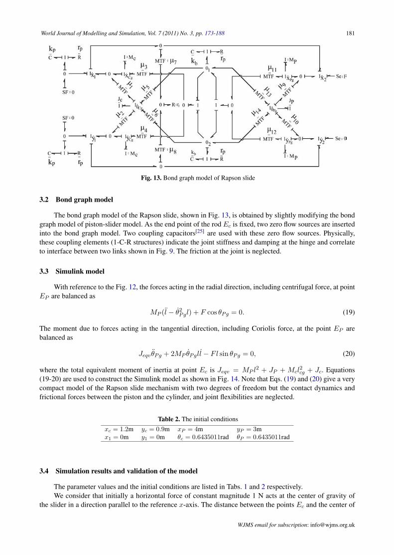
Fig. 13. Bond graph model of Rapson slide

3.2 Bond graph model

The bond graph model of the Rapson slide, shown in Fig. 13, is obtained by slightly modifying the bondgraph model of piston-slider model. As the end point of the rod Ec is fixed, two zero flow sources are insertedinto the bond graph model. Two coupling capacitors[25] are used with these zero flow sources. Physically,these coupling elements (1-C-R structures) indicate the joint stiffness and damping at the hinge and correlateto interface between two links shown in Fig. 9. The friction at the joint is neglected.

3.3 Simulink model

With reference to the Fig. 12, the forces acting in the radial direction, including centrifugal force, at pointEP are balanced as

MP (l − θ2Pgl) + F cos θPg = 0. (19)

The moment due to forces acting in the tangential direction, including Coriolis force, at the point EP arebalanced as

Jeqv θPg + 2MP θPgll − Fl sin θPg = 0, (20)

where the total equivalent moment of inertia at point Ec is Jeqv = MP l2 + JP + Mcl

2cg + Jc. Equations

(19-20) are used to construct the Simulink model as shown in Fig. 14. Note that Eqs. (19) and (20) give a verycompact model of the Rapson slide mechanism with two degrees of freedom but the contact dynamics andfrictional forces between the piston and the cylinder, and joint flexibilities are neglected.

Table 2. The initial conditionsxc = 1.2m yc = 0.9m xP = 4m yP = 3mx1 = 0m y1 = 0m θc = 0.6435011rad θP = 0.6435011rad

3.4 Simulation results and validation of the model

The parameter values and the initial conditions are listed in Tabs. 1 and 2 respectively.We consider that initially a horizontal force of constant magnitude 1 N acts at the center of gravity of

the slider in a direction parallel to the reference x-axis. The distance between the points Ec and the center of



Fig. 14. Simulink model of Rapson slide

Fig. 15. Angular displacement, velocity and acceleration for the center of the slider. Line indicates Bond graph model,and Scatter points indicate Simulink model

gravity of the piston is 5m. The angular displacement, angular velocity, and the angular acceleration of theslider are shown in Fig. 15 where lines indicate results from the bond graph model and scattered points areresults from the Simulink model. The results for the angular velocity and angular acceleration from the twomodels differ slightly. The difference in angular accelerations of the slider is shown in Fig. 16. These differ-ences are due to the contact forces and joint flexibilities modelled in the bond graph model. The accelerationerrors are significant when the joints are initially loaded (near t = 0s) and somewhat significant when the rateof acceleration is high, i.e., the motion is jerky[5] (between t = 2s to t = 6s). Without consideration of jointflexibility (i.e., when joint stiffness is large), these effects are not visible. Note that integration of accelerationerror is almost zero and hence the error between velocity profiles is significantly less. Further integration of



velocity errors yields practically no error in displacement profiles. The joint flexibilities included in the bondgraph model yield the transient forces that must be accounted for when designing the linkages for specifiedstrength and fatigue life[5].

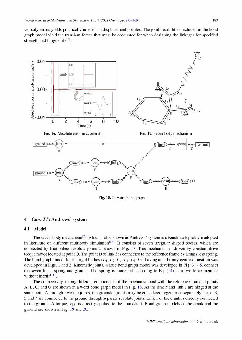
Fig. 16. Absolute error in acceleration Fig. 17. Seven body mechanism

Fig. 18. Its word bond graph

4 Case II: Andrews’ system

4.1 Model

The seven-body mechanism[23] which is also known as Andrews’ system is a benchmark problem adoptedin literature on different multibody simulation[16]. It consists of seven irregular shaped bodies, which areconnected by frictionless revolute joints as shown in Fig. 17. This mechanism is driven by constant drivetorque motor located at point O. The point D of link 3 is connected to the reference frame by a mass less spring.The bond graph model for the rigid bodies (L1, L2, L4, L5, L6, L7) having an arbitrary centroid position wasdeveloped in Figs. 1 and 2. Kinematic joints, whose bond graph model was developed in Fig. 3 ∼ 5, connectthe seven links, spring and ground. The spring is modelled according to Eq. (14) as a two-force memberwithout inertia[18].

The connectivity among different components of the mechanism and with the reference frame at pointsA, B, C, and O are shown in a word bond graph model in Fig. 18. As the link 5 and link 7 are hinged at thesame point A through revolute joints, the grounded joints may be considered together or separately. Links 3,5 and 7 are connected to the ground through separate revolute joints. Link 1 or the crank is directly connectedto the ground. A torque, τM , is directly applied to the crankshaft. Bond graph models of the crank and theground are shown in Fig. 19 and 20.



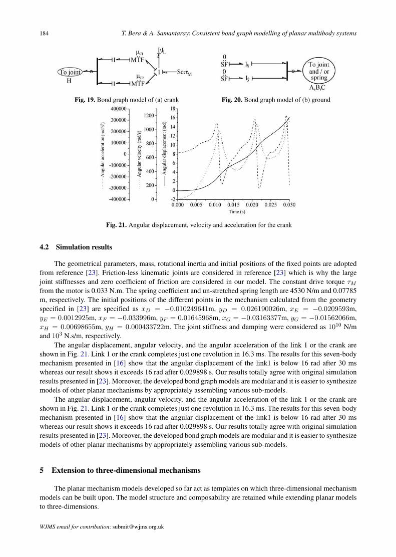
Fig. 19. Bond graph model of (a) crank Fig. 20. Bond graph model of (b) ground

Fig. 21. Angular displacement, velocity and acceleration for the crank

4.2 Simulation results

The geometrical parameters, mass, rotational inertia and initial positions of the fixed points are adoptedfrom reference [23]. Friction-less kinematic joints are considered in reference [23] which is why the largejoint stiffnesses and zero coefficient of friction are considered in our model. The constant drive torque τMfrom the motor is 0.033 N.m. The spring coefficient and un-stretched spring length are 4530 N/m and 0.07785m, respectively. The initial positions of the different points in the mechanism calculated from the geometryspecified in [23] are specified as xD = −0.010249641m, yD = 0.026190026m, xE = −0.0209593m,yE = 0.0012925m, xF = −0.033996m, yF = 0.01645968m, xG = −0.03163377m, yG = −0.01562066m,xH = 0.00698655m, yH = 0.000433722m. The joint stiffness and damping were considered as 1010 N/mand 103 N.s/m, respectively.

The angular displacement, angular velocity, and the angular acceleration of the link 1 or the crank areshown in Fig. 21. Link 1 or the crank completes just one revolution in 16.3 ms. The results for this seven-bodymechanism presented in [16] show that the angular displacement of the link1 is below 16 rad after 30 mswhereas our result shows it exceeds 16 rad after 0.029898 s. Our results totally agree with original simulationresults presented in [23]. Moreover, the developed bond graph models are modular and it is easier to synthesizemodels of other planar mechanisms by appropriately assembling various sub-models.

The angular displacement, angular velocity, and the angular acceleration of the link 1 or the crank areshown in Fig. 21. Link 1 or the crank completes just one revolution in 16.3 ms. The results for this seven-bodymechanism presented in [16] show that the angular displacement of the link1 is below 16 rad after 30 mswhereas our result shows it exceeds 16 rad after 0.029898 s. Our results totally agree with original simulationresults presented in [23]. Moreover, the developed bond graph models are modular and it is easier to synthesizemodels of other planar mechanisms by appropriately assembling various sub-models.

5 Extension to three-dimensional mechanisms

The planar mechanism models developed so far act as templates on which three-dimensional mechanismmodels can be built upon. The model structure and composability are retained while extending planar modelsto three-dimensions.



5.1 Three dimensional prismatic joint

The planar model of prismatic joint can be easily extended to three-dimensional model. The three di-mensional cylinder-piston is modelled as a rigid body with twelve degrees of freedom in which the contactbetween the cylinder and piston impose six constraints. If ideal kinematic constraints are considered then thethree dimensional cylinder-piston model has six degrees of freedom. However, we consider constraints allow-ing local deformations so as to compute normal reactions at contact points and thus to dynamically computethe frictional forces. The rigid body motion is described in body-fixed frame which is attached at the center ofmass of the rigid body and aligned with the principal axes. The Newton-Euler equations of the cylinder withattached body fixed axes aligned with the principal axes of inertia are as follows:∑

Fx = Mcxc +Mc(zcθcy − ycθcz), (21)∑Fy = Mcyc +Mc(xcθcz − zcθcx), (22)∑Fz = Mczc +Mc(ycθcx − xcθcy), (23)∑Mx = Jcxθcx + θcz θcy(Jcz − Jcy), (24)∑My = Jcy θcy + θcxθcz(Jcx − Jcz), (25)∑Mz = Jcz θcz + θcy θcx(Jcy − Jcx), (26)

where Fx, Fy and Fz are external forces acting in body-fixed x, y and z directions, respectively, Mx, My

and Mz are external moments acting in body-fixed x, y and z directions, respectively, Mc is the mass of thecylinder, Jcx, Jcy and Jcz are the moment of inertias about principal axes, xc, yc and zc are velocities ofthe mass center in the body-fixed frame, xc, yc and zc are accelerations of the mass center in the body-fixedframe, θcx, θcy and θcz are angular velocities of the mass center in the body-fixed frame, and θcx, θcy and θczare angular accelerations of the mass center in the body-fixed frame.

In the bond graph model of the three-dimensional prismatic joint shown in Fig. 22, the inertias are coupledby a pair of gyrator rings (Euler junction structures) [12, 18], one for translational and the other for rotationalvelocities, according to Eqs. (21) ∼ (26). They introduce six degrees of freedom. Likewise, six more degreesof freedom are considered for the piston and the piston rod. They are represented by another pair of gyratorrings and the variables used in that part of the model are represented by similar nomenclature where subscript’p’ used in place of ’c’ to indicate that they are associated with the piston.

The co-ordinate transformation (CTF) blocks in Fig. 22 are required to transform body fixed velocitiesto the inertial velocities. The rate of change of contemporary length (l) between cylinder end and the piston isexpressed as

l =(X1 −X2

l

)(X1 − X2) +

(Y1 − Y2

l

)(Y1 − Y2) +

(Z1 − Z2

l

)(Z1 − Z2), (27)

where (X1, Y1, Z1) represents the coordinates of the cylinder end point in the inertial frame and (X2, Y2, Z2)represents the coordinates of the piston end point in the inertial frame. The position of the cylinder end pointwith respect to the body-fixed frame at the mass center is given as (x1, y1, z1) and that for the piston endpoint with respect its body-fixed frame is given as (x2, y2, z2). The velocities of these points are representedin the bond graph model at 1-junctions with appropriate suffixes. The linear and angular velocities of the masscenters of the cylinder and piston are used to compute velocities of the end points in respective body-fixedframes and then they are transformed to inertial velocities to implement constraints in the inertial frame, i.e.,Eq. (27) and external forces (joint forces) acting at the end points of the cylinder and the piston. The end pointjoint forces are inputs to the model given at ports ¬ and .

MTF-elements with moduli µx, µy and µz are used to calculate the relative sliding velocity between thepiston and the cylinder at a 0-junction and the friction between the piston and the cylinder is modelled by an R-element at that junction. A set of transformers with moduli c1 to c4 and p1 to p4 are determined from kinematicanalysis to compute the velocities of the contact points on the cylinder and the piston in respective body-fixed



Fig. 22. Bond graph model of three dimensional prismatic joint



Fig. 23. Bond graph model of three dimensional revolute joint

frames. These body-fixed velocities are transformed to inertial velocities (through a set of transformers withmoduli µ1 to µ12) and are then implicitly constrained. The normal velocity at the contact point on the cylinderis made equal to normal velocity at the contact point on the piston by providing higher values of contactstiffness and damping parameters, kb and rb, respectively. In comparison to other stiffness at the contact point,the bending stiffness of the piston rod is lowest and hence kb and rb and are approximated to represent thebending stiffness and damping of the piston rod.

5.2 Three dimensional revolute joint

The bond graph model of three-dimensional revolute clearance joint in compact form using vector bondsis shown in Fig. 23. The constitutive relation for the RC-field element (a field element is connected to morethan one bonds) is e = ϕRC(f ,

∫fdt) where r is a set of fixed parameters (geometric and material properties),

f = [x1, y1, z1, φ1, ψ1, θ1, x2, y2, z2, φ2, ψ2, θ2, ]T is the vector of generalized flow (velocity) variables, e =[Fx1 , Fy1 , Fz1 ,Mx1 ,My1 ,Mz1 , Fx2 , Fy2 , Fz2 ,Mx2 ,My2 ,Mz2 ]

T is the vector of generalized effort variablesand ϕRC(.) function models the constitutive relation of the joint.

6 Conclusions

Bond graph modelling of planar mechanical systems consisting of rigid body components and revolutejoints was considered in this paper. Thereafter, the bond graph model of a joint with looseness was developedto model the impact forces due to joint clearance. The main objective of this article was to develop composablesub-models of a planar mechanical library which can be easily integrated to create the model of a complexmechanism and mass distribution in prismatic or slider joints are developed. A generalized model of a slidercomponent with two moving contact points was developed from the first principles. We have developed themodels in such a way that by varying suitable geometrical parameter values, various mechanism configurationscan be represented. Two separate case studies, a Rapson slide and a seven-body mechanism, are considered tovalidate the developed models. It has been shown that the planar joint models can be extended easily to formthree-dimensional joint models.

This paper does not merely explain some particular mechanism, but forms a basis for development of amechanism library by using bond graph models. The models developed in the article are modular, i.e., theycan be easily interfaced with other models and extended by adding other dynamical parts. Mechanisms areoften used with other devices, e.g., the slider-crank mechanism connects the IC engine to the fluid coupling ofthe automatic transmission system of a vehicle. The multi-energy domain representation through bond graphmodelling allows for integration of electrical, hydraulic/ pneumatic and thermal domains, etc. into the model.

References

[1] S. Ahmed, H. Lankarani, M. Pereira, Frictional impact analysis in open-loop multibody mechanical systems.Journal of Mechanical Design, Transactions of the ASME, 1999, 121(1): 119–127.

[2] J. Baumgarte. Stabilization of constraints and integrals of motion in dynamical systems. Computer Methods inApplied Mechanics and Engineering, 1972, 1: 1–16.

[3] W. Borutzky. Bond Graphs—A Methodology for Modelling Multidisciplinary Dynamic Systems. SCS PublishingHouse, San Diego, 2004.

[4] G. Dauphin-Tanguy. Les Bond Graphs. Hermes Science Europe Ltd, Paris, 2000.[5] S. Erkaya, I. Uzmay. Investigation on effect of joint clearance on dynamics of four-bar mechanism. Nonlinear

Dynamics, 2009, 58(1-2): 179–198.



[6] A. Filippov. Vibrations of Mechanical systems. National Lending Library for Science and Technology, Boston Spa,Yorkshire, England, 1971.

[7] P. Flores. Modeling and simulation of wear in revolute clearance joints in multibody systems. Mechanism andMachine Theory, 2009, 44(6): 1211–1222.

[8] P. Flores, J. Ambrosio, et al. Kinematics and Dynamics of Multibody Systems with imperfect joints: Models andcase studies. Springer, Berlin/Heidelberg, 2008.

[9] P. Gawthrop, L. Smith. Metamodelling: Bond Graphs and Dynamic Systems. Prentice Hall, 1996.[10] D. Karnopp. Computer simulation of stick-slip friction in mechanical dynamic systems. Journal of Dynamic

Systems, Measurement and Control, Transactions of the ASME, 1985, 107(1): 100–103.[11] D. Karnopp, D. Margolis. Analysis and simulation of planar mechanism systems using bond graphs. Journal of

Mechanical Design, 1979, 101(2): 187–191.[12] D. Karnopp, D. Margolis, R. Rosenberg. System Dynamics: Modeling and Simulation of Mechatronic Systems.

John Wiley & Sons Incorporated, 2006.[13] R. Kubler, W. Schiehlen. Modular simulation in multibody system dynamics. Multibody System Dynamic, 2000,

4(2-3): 107–127.[14] I. Khemili, L. Romdhane. Dynamic analysis of a flexible slider-crank mechanism with clearance. European Journal

of Mechanics, A/Solids, 2008, 27(5): 882–898.[15] W. Marquis-favre, E. Bideaux, S. Scavarda. A planar mechanical library in the amesim simulation software. part i:

Formulation of dynamics equations. Simulation Modelling Practice and Theory, 2006, 14(1): 25–46.[16] W. Marquis-favre, E. Bideaux, S. Scavarda. A planar mechanical library in the amesim simulation software. part

ii: Library composition and illustrative example. Simulation Modelling Practice and Theory, 2006, 14(2): 95–111.[17] J. McPhee. On the use of linear graph theory in multibody system dynamics. Nonlinear Dynamics, 1996, 9(1-2):

73–90.[18] A. Mukherjee, R. Karmakar, A. Samantaray. Bond Graph in Modeling, Simulation and fault Identification. CRC

Press, Florida, 2006.[19] M. Otter, H. Elmqvist, F. Cellier. Modeling of multibody systems with the object-oriented modeling language

dymola. Nonlinear Dynamics, 1996, 9(1): 91–112.[20] A. Sagirli, M. Bogoclu, V. Omurlu. Modeling the dynamics and kinematics of a telescopic rotary crane by the bond

graph method (part i). Nonlinear Dynamics, 2003, 33: 337–351.[21] A. Samantaray, R. Bhattacharyya, A. Mukherjee. An investigation into the physics behind the stabilizing effects of

two-phase lubricants in journal bearings. Journal Vibration and Control, 2006, 12(4): 425–442.[22] S. Sandhu, J. McPhee. Partitioned dynamic simulation of multibody systems. Journal of Computational and

Nonlinear Dynamics, 2010, 5(3): 1–7.[23] W. Schiehlen. Multibody Systems Handbook. Springer Verlag, Berlin, 1990.[24] W. Schiehlen. Multibody system dynamics: Roots and perspectives. Multibody System Dynamics, 1997, 1: 149–

188.[25] J. Thoma, B. Bouamama. Modelling and Simulation in Thermal and Chemical Engineering. Springer-Verlag, New

York, 2000.[26] Q. Tian, Y. Zhang, et al. Simulation of planar flexible multibody systems with clearance and lubricated revolute

joints. Nonlinear Dynamics, 2010, 60: 489–511.


consistent bond graph modelling of planar multibody systems · 174 t. bera & a. samantaray:...

Documents