From the SelectedWorks of Kathy Baylis

2016

Conservation Agriculture and Climate ResilienceJeffrey Michler, University of Illinois at Urbana-ChampaignKathy BaylisMary Arends-Kuenning, University of Illinois at Urbana-ChampaignKizito Mazvimavi, International Crop Research Institute in the Semi-Arid Tropics

Available at: https://works.bepress.com/kathy_baylis/77/

Conservation Agriculture and Climate Resilience

Jeffrey D. Michler∗a,b, Kathy Baylisa, Mary Arends-Kuenninga, and Kizito Mazvimavib

aUniversity of Illinois, Urbana, USAbInternational Crops Research Institute for the Semi-Arid Tropics, Bulawayo, Zimbabwe

November 2016

Abstract

Climate change is predicted to increase the number and severity of extreme rainfall events, espe-cially in Sub-Saharan Africa. In response, development agencies are encouraging the adoption of‘climate-smart’ agricultural techniques, such as Conservation Agriculture (CA). However, littlerigorous evidence exists to demonstrates the effect of CA on production or climate resilience,and what evidence there is, is hampered by selection bias. Using panel data from Zimbabwe, wetest how CA performs during extreme rainfall events - both shortfalls and surpluses. We controlfor the endogenous adoption decision and find that while CA has little, or if anything, a nega-tive effect on yields during periods of average rainfall, it is effective in mitigating the negativeimpacts of rainfall shocks. Farmers who practice CA tend to receive higher yields compared toconventional farmers in years of both low and high rainfall. We conclude that the lower yieldsduring normal rainfall seasons may be a proximate factor in low uptake of CA. Policy shouldfocus promotion of CA on these climate resiliency benefits.

JEL Classification: O12, O13, Q12, Q54, Q56

Keywords: Conservation Farming; Technology Adoption; Agricultural Production; Resilience, Weather Risk;

Zimbabwe

∗Corresponding author email: jmichler@illinois.edu. The authors owe a particular debt to Albert Chiima, TarisayiPedzisa, and Alex Winter-Nelson. This work has benefited from helpful comments and criticism by Anna Josephson,David Rohrbach, David Spielman, and Christian Thierfelder as well as seminar participants at the AAAE conferencein Addis Ababa. We gratefully acknowledge financial support for the data collection from the United KingdomDepartment for International Development (DFID) and United Nations Food and Agriculture Organization (FAO)through the Protracted Relief Program (PRP) in Zimbabwe, 2007-2011. Additional funding support is from theStanding Panel on Impact Assessment of the CGIAR.

1 Introduction

Conservation agriculture (CA) is a cropping system based on three principles promoted as a means

for sustainable agricultural intensification. These practices include minimum soil disturbance (no-

till), mulching with crop residue, and crop rotation. The goal of these practices is to provide a

variety of benefits to farmers including increased soil fertility, reduced input demand, and reduced

risk to yields from rainfall shocks (Brouder and Gomez-Macpherson, 2014). This last benefit comes,

in the case of sub-optimal rainfall, through the use of planting basins, in combination with mulching,

which increases water infiltration and moisture conservation (Thierfelder and Wall, 2009), while,

in the case of excess rainfall, through the retention of crop residue, which reduces erosion rates

(Schuller et al., 2007). As a result, CA has become a prominent component of global agricultural

development policy to sustainably increase crop productivity, and a fixture in the promotion of

‘climate smart’ agriculture (FAO, 2011).1 Yet little evidence exists regarding CA’s ‘climate smart’

properties (Andersson and D’Souza, 2014). A few studies explore the effect of CA on yields during

normal rainfall years, but these studies either use agronomic analysis of field station trials, missing

potential effects of farmer behavior, or use observational data that fail to control for the selection

bias in the adoption decision (Pannell et al., 2014).

We examine CA’s ability to reduce yield loss due to deviations in average rainfall, while con-

trolling for potential selection bias. While CA is hypothesized to be ‘climate smart,’ increased

resiliency during periods of rainfall stress may come at the cost of yields during regular growing

conditions. Additionally, the resilience of yields under CA may differ depending on if farmers ex-

perience rainfall shortages or rainfall surpluses. We follow Di Falco and Chavas (2008) in defining

resilience in terms of a set of agricultural practices that retain their productivity when challenged

by climatic events. To test the resilience of yields on fields where farmers practice CA we use four

years of plot level panel data covering 4, 217 plots from 730 households across Zimbabwe. The data

include plot level inputs and outputs for five different crops: maize, sorghum, millet, groundnut,

1FAO (2013) broadly defines climate smart agriculture (CSA) as an approach to agriculture designed to helpfarmers effectively respond to climate change. More narrowly, the role of CA as a ‘climate smart’ technology isthrough its proposed ability to build resilience to climate change and reduce greenhouse gas emissions throughcarbon sequestration.

1

and cowpea. Unlike earlier work that estimates CA’s effect on a single crop, this rich set of produc-

tion data allows us to examine how the impacts of CA vary in the multi-cropping system common

to Sub-Saharan Africa.

Causal identification of CA’s impact on yields is complicated by non-random adoption of the

technology. We identify two potential sources of endogeneity that might bias our results. First is

the presence of household heterogeneity that influences both adoption and yields but is otherwise

unobserved. We employ household fixed effects to control for correlation between time-invariant

unobservables and the choice to adopt CA. Second is the possible presence of unobserved time-

varying shocks captured in the error term that might affect a household’s access to and use of

CA. We use the intensity of nearby CA promotion to instrument for household adoption of CA. In

addition to these two primary concerns, we test for other potential factors that could confound the

causal identification of CA on yields. Because farmers do not use CA on their entire farm, the choice

of which plots to use for CA might be endogenous. To test this concern, we use a subset of our

data for which we have consistent plot identifiers and estimate plot level fixed effects regressions.

In our data, we find that adoption of CA in years of average rainfall results in no yield gains, and

in some cases yield loses, compared to conventional practices. Where CA is effective is in mitigating

the negative impacts of deviations in rainfall. CA results in yields that are more resilient to these

rainfall shocks than yields using conventional farming methods for maize and cowpea. The climate

resilience of crops under CA is robust to the disaggregation of rainfall shocks into shortages and

surpluses and to the inclusion of plot level effects. We then use the estimated coefficients on the CA

terms to predict the returns to CA at various values for rainfall. Just over a half standard deviation

decrease or increase in rainfall is required before the returns to CA become positive. Under average

rainfall conditions, overall returns to CA are negative. Our results, using observational data,

support a recent meta-analysis of agronomic field experiments which found that, on average, CA

reduces yields but can enhance yields in dry climates (Pittelkow et al., 2015).

Pannell et al. (2014) discuss several limitations with the state of research on the economics of

CA at the farm or plot level. A key limitation is a lack of clarity regarding what qualifies as CA

adoption. Our survey data only allow us to partially address this concern. While the data cover

2

four cropping seasons, in the first two seasons (2008 and 2009) households simply identified the

plots on which they practiced CA. Only in the final two seasons (2010 and 2011) were households

asked to specify which practices they implemented when using CA. Among households that used

CA in the last two years of the survey, 97 percent of them used planting basins to achieve minimum

soil disturbance, 27 percent mulched with crop residuals, and 36 percent practiced crop rotation.

In total, 22 percent of self-identified CA adopters engaged in at least two practices while only

five percent of CA adopters actually engaged in all three practices. Therefore, in our context, we

operate with a practical definition of CA as, at the very least, use of no-till, the original and central

principle of CA. We then define conventional or traditional cultivation practices as everything other

than self-identified CA adoption, which for the majority of plots amounts to tillage by ox-drawn or

tractor plows. While our pragmatic approach is not ideal, it is in line with previous literature at

the farm level and with meta-analyses of agronomic field experiment data.2

This paper makes three contributions to the literature. First, by interacting the instrumented

measure of CA adoption with deviations in rainfall we test whether CA can help mitigate yield

loss due to adverse weather events. The ability to mitigate yield loss from rainfall shocks has been

a key proposed benefit of CA (Giller et al., 2009) and evidence exists that farmers who adopt CA

do so with the expectation that CA will provide resilient yields (Arslan et al., 2014). Yet, the only

evidence of the resilience of yields under CA comes from station or on-farm field trial data.3 We

use realizations of on-farm yields over four years and control for several sources of endogeneity.

Thus we provide the first rigorous evidence about CA’s ‘climate smart’ properties.

Second, we expand the analysis of CA by encompassing a variety of crops. Most previous

work focuses on the impact of CA on yields for a single crop, often maize (Brouder and Gomez-

Macpherson, 2014). But, farmers in Sub-Saharan Africa frequently grow multiple crops in a single

season, meaning decisions regarding cultivation method and input use are made at the farm level,

not the crop level. To examine the farm-wide impacts, we adopt a flexible production function that

allows coefficients on inputs to vary across crops. This approach accommodates heterogeneity in

2Using the last two years of the data, we test how the individual practices, singly and in combinations, impactyields during periods of rainfall stress. Results are not significantly different from our broader measure of CA.

3Recent examples include Thierfelder et al. (2013) and Thierfelder et al. (2015). See Corbeels et al. (2014) for areview of this literature.

3

the input-response curves by allowing slopes and intercepts to vary across crops without forcing us

to split the random sample based on non-random criteria. Our results provide new insight on the

use and impact of CA in a multi-cropping environment.

Third, we provide suggestive evidence on the reason for the low adoption rate of CA among

farmers in Sub-Saharan Africa. Given early evidence on the positive correlation between CA and

yields (Mazvimavi and Twomlow, 2009), and its promotion by research centers, donor agencies, and

policymakers (Andersson and D’Souza, 2014), the slow uptake of CA has presented the adoption

literature with an empirical puzzle. We find that once we control for endogeneity in the adoption

decision, CA no longer has any impact on yields during periods of average rainfall. We conclude

that the lack of yield gains during average rainfall seasons may be a limiting factor in the uptake

of CA. Focusing on CA’s potential as a ‘climate smart’ agricultural technology by advertising the

resilience benefits of CA marks a path forward for the promotion of CA in regions facing climate

extremes.

2 Theoretical Framework

We begin by defining a stochastic production function:

ykit = f(x kit; c )eεkit , (1)

where ykit is yield for crop k cultivated by household i at time t, x kit is a vector of measured inputs

used on the kth crop by household i at time t, and c is a vector of other factors that include CA,

rainfall, and their interaction. The disturbance term is composed of two elements: εkit = µi + ukit.

We assume both µi and ukit are independently distributed. The µi reflects unobserved household

level effects that impact the production technology while ukit ∼ N (0, σ2ukit

).

We consider the following specification:

ln(ykit) = αk + ln(x kit)βk + φk0C kit + φk1R kjt + φk2C kit · R kjt + µi + ukit, (2)

where αk is a crop-specific intercept term and βk is a vector of crop-specific coefficients to be

4

estimated for the input vector x kit. Our variables of interest are the indicator variable C kit for

whether or not CA methods were used by household i in cultivating crop k at time t, along with

our measure of rainfall deviations, R jt, calculated for ward j at time t, and the interaction term,

C kit · R kjt. The φ terms are estimated coefficients which will allow us to test the impact of CA

on yields both during times of average rainfall (φk0) and during periods of deviation from the

average (φk2). In our empirical implementation we instrument for the likely endogeneity of the C

term using an approach outlined by Wooldridge (2003). We discuss this approach more fully in

Section 4.

Note that the specification in equation (2) reduces to a Cobb-Douglas function when φk0 =

φk1 = φk2 = 0. While it is recognized that the Cobb-Douglas is not a flexible functional form,

in studies of developing country agriculture it is often still preferred to the translog due to data

limitations, the simplicity of the production technology, and the frequent issue of multicollinearity

in estimation (Michler and Shively, 2015). To allow for some flexibility in production we relax the

assumption of constant returns to measured inputs and allow the input-response curves to vary

by crop. We also include both the levels and the interaction of CA and the rainfall measures

and allow these coefficients to vary by crop. Since these interactions are our variables of interest,

this estimation approach gives us a flexible specification where we believe it matters most, while

maintaining a degree of parsimony in our equation of estimation.

3 Data

This study uses four years of panel data on smallholder farming practices in Zimbabwe collected by

the International Crops Research Institute for the Semi-Arid Tropics (ICRISAT). The data cover

783 households in 45 wards from 2007-2011.4 The wards come from 20 different districts which

were purposefully selected to provide coverage of high rainfall, medium rainfall, semi-arid, and arid

regions (see Figure 1). Thus the survey can be considered nationally representative of smallholder

agriculture in Zimbabwe. For our analysis we use an unbalanced panel consisting of a subset of 730

randomly selected households. The 53 excluded households come from the 2007 round, which we

4Wards are the smallest administrative district in rural Zimbabwe.

5

drop completely, because in that year the survey only targeted households who had received NGO

support that was designed to stimulate CA adoption.

3.1 Household Data

Our subset provides us with detailed cultivation data for five crops on 4, 217 unique plots (see

Table 1). Maize, the staple grain of Zimbabwe, is the most commonly cultivated crop. Nearly half

of all observations are maize and 98 percent of households grow maize on at least one plot in every

year. The next most common crop, in terms of observations, is groundnut, which is often grown

in rotation with maize. The third most common crop is sorghum, which is frequently grown as

an alternative to maize in the semi-arid regions of Zimbabwe. As an alternative to groundnut and

sorghum, households will often grow cowpea or pearl millet, respectively. Both of these crops are

much less common and combine to account for only 15 percent of observations.

In Table 2 we explore the differences in outputs and input use by crop across cultivation prac-

tices.5 Mean yields for all crops are significantly higher under CA than under traditional cultivation

methods. Turning to inputs, we find that CA maize production uses more fertilizer but less seed

and the area under CA is less than the area under traditional cultivation. This same pattern of

input use is repeated for all the other crops. The higher yields for most crops under CA is correlated

with more intensive fertilizer use and, once having controlled for fertilizer use, CA might not have

an effect on yields. We more fully explore these relationships in our econometric analysis below.

Figure 2 shows the distribution of yields over the period 2008-2011 by cultivation method and by

rainfall. In seasons when rainfall is normal, mean yields are larger under CA compared to traditional

cultivation.6 Using the Kolmogorov-Smirnov test we reject the equality of yield distributions for CA

and traditional cultivation under normal conditions with 99 percent confidence.7 When we examine

5For each crop-cultivation pair we first test for normality of the data using the Shapiro-Wilk test. In every casewe reject the null that the data is normally distributed. Because of this, we rely on the Mann-Whitney-Wilcoxon(MW) test instead of the standard t-test to determine if differences exist within crops across cultivation practices.Unlike the t-test, the MW test does not require the assumption of a normal distribution. In the context of summarystatistics we also prefer the MW test to the the Kolmogorov-Smirnov (KS) test, since the MW test is a test of locationwhile the KS test is a test for shape. Results using the KS test are equivalent to those obtained from the MW test.

6We define normal as cumulative seasonal rainfall that is within one standard deviation of mean seasonal rainfall.The mean and standard deviation of seasonal rainfall is calculated using rainfall data from the last 15 years. Wedefine abnormal as cumulative seasonal rainfall that is more than one standard deviation away from the mean.

7In the context of marginal distributions we prefer the KS test to the MW test since the KS test is sensitive to

6

yields during periods of abnormal rainfall, mean yields are again larger under CA. Additionally,

the variance in CA yields is lower than the variance of yields under traditional cultivation. Using

the Kolmogorov-Smirnov test, these differences are significant at the 99 percent level. Focusing

just on CA yields, we observe only a small difference in mean yields during normal and abnormal

rainfall seasons, although we still reject the equality of these distributions at the 90 percent level.

Conversely, we observe a much larger difference in mean yields from traditional cultivation for

periods of normal rainfall compared to abnormal rainfall (we reject the null of equality with 99

percent confidence). This descriptive evidence suggests that CA may contribute to yield resilience

during periods of rainfall shock. Note that these graphs do not imply a causal relation between

cultivation methods and yields since they fail to account for potential selection bias in households

that adopt CA.

Examining the production data by year reveals a high degree of annual variability (see Table 3).

Yields in 2009 and 2010 were about 50 percent higher than yields in 2008 or in 2011, despite the

much higher levels of fertilizer and seed use in the low yield years. CA practices vary both by crop

and over time (see Figure 3). In 2008, adoption of CA was at over 50 percent for those cultivating

sorghum, groundnut, and cowpea and it was 45 percent for those cultivating maize. Since then

adoption of CA has declined for all crops so that the average adoption rate is now only 17 percent,

although use of CA for maize cultivation remains relatively high at 25 percent of households.

Previous literature has hypothesized that this abandonment of CA by farmers in Zimbabwe is due

to the withdrawal of NGO input support subsequent to the 2008 economic crisis (Ndlovu et al.,

2014; Pedzisa et al., 2015). We make use of this insight to help identify CA adoption.

3.2 Rainfall Data

To calculate rainfall shocks we use satellite imagery from the Climate Hazards Group InfraRed

Precipitation with Station (CHIRPS) data. CHIRPS is a thirty year quasi-global rainfall dataset

that spans 50◦S-50◦N, with all longitudes. CHIRPS incorporates 0.05◦ resolution satellite imagery

with in-situ station data to create a gridded rainfall time series. More details are available in Funk

any differences in the two distributions (shape) and not just to differences in location. We also test for differencesusing the MW test. Results are equivalent to those obtained from the KS test.

7

et al. (2015). The dataset provides daily rainfall measurements from 1981 up to the current year.

We overlay ward boundaries on the 0.05◦ grid cells and take the average rainfall for the day within

the ward. We then aggregate the ward level daily rainfall data to the seasonal level, where the

growing season in Zimbabwe lasts from October until April the following year.

Figure 4 shows historic seasonal rainfall distribution by ward over the 15 year period 1997-

2011. We observe a large seasonal fluctuation as well as longer term cycles in rainfall patterns. The

four-year period 1997-2000 saw relatively high levels of rainfall. This was followed by a six-year

period in which rainfall was relatively scarce. Since 2007, and throughout the survey period, rainfall

was again relatively abundant. In addition to plotting the ward-level realization, we fit a linear

trendline to the data.8 Over the last 15 years, despite the long term cycles, seasonal rainfall levels

have been decreasing in Zimbabwe. To determine the degree of variation in realized rainfall over

the four year study period, we draw the distribution of cumulative seasonal rainfall (see Figure 5).

The distribution forms a fairly tight band, with half the observations (51 percent) falling within

half a standard deviation of the mean and a majority of observations (71 percent) falling within

one standard deviations of the mean.

We follow Ward and Shively (2015) in measuring rainfall shocks as normalized deviations in a

single season’s rainfall from expected seasonal rainfall over the 15 year period 1997-2011:

R jt =

∣∣∣∣rjt − rjσrj

∣∣∣∣ . (3)

Here shocks are calculated for each ward j in year t where rjt is the observed amount of rainfall for

the season, rj is the average seasonal rainfall for the ward over the period, and σrj is the standard

deviation of rainfall during the same period.

Our rainfall shock variable treats too little rain as having the same effect as too much rain.

While this may not appear to be meaningful in an agronomic sense, proponents of CA claim that

CA will have a positive impact on yields in both abnormally wet and abnormally dry conditions

(Thierfelder and Wall, 2009). To understand the validity of these claims we also calculate a measure

of rainfall shortage as:

8The slope of this line is −3.71 and is significantly different from zero at the 99 percent level.

8

R jt =

∣∣∣ rjt−rjσrj

∣∣∣ if rjt < rj

0 otherwise

, (4)

as well as a measure of rainfall surplus:

R jt =

∣∣∣ rjt−rjσrj

∣∣∣ if rjt > rj

0 otherwise

. (5)

These measures can help clarify if CA’s impact on yield resilience is primarily due to mitigating

loss from drought or from excess rainfall.

One potential concern with our rainfall terms is that they are measures of deviations in mete-

orological data which are designed to proxy for agricultural drought or overabundance of rainfall.

In Zimbabwe, agricultural drought frequently takes the form of late onset of rains or mid-season

dry spells. A further complication is that rainfall in Zimbabwe is often of high intensity but low

duration and frequency, creating high runoff and little soil permeation. To test for this, we examine

the impact of both seasonal and monthly deviations in rainfall on crop output. For all five crops,

deviations in seasonal rainfall have a significant and negative impact on crop yields. By contrast,

we find little empirical evidence that late onset of rainfall decreases crop yields and only minor

evidence that mid-season dry spells reduce yields. Results from these regressions are presented

in the Online Appendix, Table A1. Based on these results we conclude that our use of seasonal

deviations is a strong proxy for rainfall induced stresses to agricultural production.

4 Identification Strategy

Identification of the impact of CA on yields is confounded by two potential sources of endogeneity.

First, time-invariant unobserved household level characteristics might influence both CA adoption

and yields. Second, time-variant unobserved shocks captured in ukit may simultaneously affect the

adoption decision and crop yields.

The first source of endogeneity may arise because some households have greater skill at farming

9

or are less risk averse and therefore more likely to adopt CA. We address this issue by incorporating

household fixed effects in our estimation of equation (2). Fixed effects remove any unobserved time-

invariant household effects that may be correlated with both the µi term, the decision to adopt,

and yields.

We next deal with the presence of unobserved shocks that simultaneously affect the idiosyncratic

error term, the decision to adopt, and yields. Because adoption of CA is not random, it is likely to

be correlated with unobserved time-varying factors, such as external promotion of CA, that may

simultaneously influence yields. In the particular case of Zimbabwe, CA was heavily promoted by

agricultural research stations, extension agents, and NGOs. This promotion often took the form of

direct support for input purchases or technical training (Mazvimavi et al., 2008). Thus, adoption of

CA is strongly correlated with having received external support (Mazvimavi and Twomlow, 2009;

Ndlovu et al., 2014; Pedzisa et al., 2015). Because the intensity of promotion and the level of

support changed from year to year adoption of CA is neither random nor static and therefore is

likely correlated with unobserved time-varying factors.

To address the endogeneity of CA we implement an instrumental variables approach. An appro-

priate instrument for this model must be correlated with a household’s decision to adopt CA but be

uncorrelated with plot yields except through the treatment. As Mazvimavi and Twomlow (2009)

and Ndlovu et al. (2014) demonstrate, there is a strong correlation between the probability that a

household adopts CA and their receiving assistance from an NGO in the form of input subsidies.

While having received NGO support is plausibly exogenous at the household level, it could be that

NGOs target individual households based on some time-varying unobservable.9 We take an added

precaution and instead use as the instrument the number of households in a ward in a given year

that receive input support from an NGO, excluding the household under consideration. The level of

support that other households receive is correlated with a given household receiving NGO support

but does not directly impact that household’s plot level yields, especially once we control for local

conditions.10 Thus, the number of households in the ward that receive NGO support satisfies the

9Note that if NGOs target based on time-invariant characteristics, such as wealth or ability, our use of fixed effectscontrol for this, making the use of household level NGO support a valid instrument.

10One may be concerned with potential spillover effects, in that a farmer who adopts CA due to NGO supportmight result in increased yields for a neighbor. For the case of CA in Zimbabwe this is unlikely for two reasons.

10

exclusion restriction.

Given that the problematic term, C it, is interacted with either crop type (to give C kit) or with

crop type and the exogenous rainfall shock (to give C kit · R kjt), we follow Wooldridge (2003) in

instrumenting for only the potentially endogenous term. We estimate a version of equation (2) in

which CA and the CA interaction terms are instrumented using the number of households in the

ward that receive NGO support. Specifically, we use a probit to predict C it from the following

equation:

C it = 1 [αk + ln(x kit)βk + γG jt + δk1R kjt + µi + vit ≥ 0] , (6)

where G jt is the number of other households in ward j that received NGO support at time t,

γ is the associated coefficient, and vit ∼ N (0, σ2vit) and is independent of uit and µi. Since our

first stage reduced form equation is nonlinear, we use correlated random effects to control for

household unobservables instead of the fixed effects used in the second stage structural equation.11

This amounts to replacing µi with its linear projection onto the time averages of observable choice

variables µi = x iλ+ai, where ai ∼ N (0, σ2ai) (Mundlak, 1978; Chamberlain, 1984). Using correlated

random effects allows us to avoid the incidental variable problem created by using fixed effects in a

nonlinear model while still controlling for unobservables (Wooldridge, 2010). While our first stage

and second stage equations take different approaches to controlling for µi, identification of C it still

fully relies on our instrumental variable G jt. Any difference that exists between the fixed effects

and the correlated random effects is captured in ai, which in expectation has zero mean. Our use

of correlated random effects will be less efficient than fixed effects to the extent that σ2ai > 0, but

this introduces no bias into our IV estimate of C it.

We then calculate the Inverse Mills Ratio (IMR) and instrument C kit with the IMR interacted

with crop type and instrument C kit ·R kjt with the IMR interacted with crop type and the exogenous

First, the practices that constitute CA are location specific, in that use of planting basins or residue or rotation onone plot will have no impact on the productivity of another plot. Second, even if this was not the case, households inthe survey are relatively dispersed throughout wards, meaning that the plots of one farmer are not contiguous withneighboring farmers.

11In the Online Appendix, Tables A8 and A9, we present results from a robustness check using a Tobit andhousehold fixed effects for the first stage.

11

rainfall shock. Wooldridge (2003) shows that this approach produces consistent estimates and

improves on efficiency when compared to instrumenting the entire interaction term.

To ensure correct hypothesis testing, we allow the variance structure of the error term to vary

by household as well as by crop and cluster our standard errors at the household-crop level. This

procedure is not without its critics. Bertrand et al. (2004) suggest that clustering at a single level is

preferred to clustering at two levels. This provides two alternatives: cluster only at the household

level or cluster only at the crop level. Clustering at the household level provides results qualitatively

equivalent to those when we cluster at the household-crop level.12 Given that we only have five

different crops, and a large set of parameters to estimate, we are unable to directly cluster standard

errors at just the crop level. Instead, in a robustness check, we estimate a system of crop-specific

production functions and allow for correlation across crops.

5 Results

We estimate the production function in equation (2) by regressing yields for each crop on crop-

specific inputs, CA, deviations from average rainfall, and their interaction. We present the results

from a large complement of estimates in Tables 4 - 9. All models are estimated using the log of

yield as the dependent variable and log values of measured inputs as independent variables. Hence,

point estimates can be read directly as elasticities. Given the prevalence of zero values in the input

data, and to a lesser extent in the output data, we use the inverse hyperbolic sine transformation

to convert levels into logarithmic values. For brevity, we only report coefficients on CA, the rainfall

deviations, and the interaction terms. Estimated coefficients on measured inputs are presented in

the Online Appendix.

5.1 Main Results

We first focus on the results presented in Table 4 in which CA is treated as exogenous. While it

is unlikely that the decision to adopt CA is uncorrelated with the time-varying error term, these

results are informative as they allow us to directly compare our estimates with previous literature

12Results from these regressions are available from the authors upon request.

12

on the correlation between CA and yields. Column (1) presents a simple production function

that lacks both our rainfall variable and household fixed effects. Results in column (2) come from

the same regression but with fixed effects to control for time-invariant household unobservables.

The correlation between CA and yields is positive and significant for maize both with and without

household fixed effects. CA is positively correlated with groundnut yields but only when we include

household fixed effects. In all other crop cases CA has no statistically significant association with

yields.

Adding deviations from average rainfall and its interaction with CA tells a very different story.

Columns (3) and (4) present point estimates of the more flexible production function with and

without fixed effects. Focusing on the fixed effects results in column (4), CA by itself no longer

increases yields for maize or groundnut. CA is now correlated with lower yields for sorghum.

Exposure to a rainfall shock decreases yields for all crops. When we examine the interaction terms,

we find that CA is correlated with higher yields for maize and sorghum during periods of rainfall

stress.

The results in columns (1) and (2) of a positive correlation between maize yields and CA are

similar to the results presented in much of the previous literature (Mazvimavi and Twomlow, 2009;

Brouder and Gomez-Macpherson, 2014; Ndlovu et al., 2014; Abdulai, 2016). These positive and

statistically significant correlations are often interpreted as demonstrating that CA increases yields

compared to traditional cultivation practices and are used to justify the continued promotion of

CA (Giller et al., 2009). However, we find that this result is not robust to the inclusion of rainfall

measures. Additionally, we expect this result to be biased due to correlation between the decision

to adopt and the error term.

Table 5 presents first stage results from the IV regression. For all four specifications our instru-

ment is positive and significantly correlated with the choice to adopt CA. In Table 6 we present

results similar to those in Table 4 but with the endogeneity of CA controlled for with our instru-

ment. Our preferred specification is column (4) because it simultaneously controls for unobserved

shocks through the IV and unobserved heterogeneity through fixed effects. We find that CA, by

itself, decreases yields on maize and provides no significant advantage over traditional cultivation

13

practices for the other crops. Similar to the results in column (4) of Table 4, we find that rainfall

deviations reduce yields on all crops.

While the lack of impact of CA on yields is discouraging, it is not the full story.13 When we

examine the interaction between CA and rainfall we find that CA increases yields in times of rainfall

stress for maize and cowpea. The use of CA during periods of rainfall stress appears to have no

benefit for sorghum, millet, and groundnut yields. For all crops, except sorghum, the coefficients

on our instrumented variables are of a larger magnitude then the un-instrumented variables. Once

we have controlled for the endogeneity of the adoption decision, the coefficients on CA tend to be

more negative while the coefficients on the interaction terms tend to be more positive. The bias

generated from not controlling for the endogeneity of CA appears to underestimate the impact,

either positive or negative, of CA on yields. Having controlled for the bias, we conclude that

smallholder farmers in Zimbabwe who cultivate their crops using CA practices receive higher yields

compared to conventional farmers but only in times of rainfall stress.

5.2 Alternative Rainfall Measures

While our main results provide evidence that CA cultivation during deviations from average rainfall

helps mitigate crop loss, our measure of rainfall deviations is agnostic to whether or not the shock

is from surplus rainfall or a shortage of rainfall. While proponents of CA claim that CA will have

a positive impact on yields in both abnormally wet and abnormally dry conditions, there is reason

to believe that CA may be more effective in one situation compared to the other, depending on the

crop in question.

Table 7 presents results from three regressions all of which treat CA as endogenous and include

household fixed effects. Column (1) shows results from the regression with the rainfall shock

measured as a shortage as in equation (4). Column (2) replaces the rainfall shortage with a rainfall

surplus as in equation (5). Column (3) uses both rainfall shortage and surplus measures. This last

specification is our preferred one because it includes the full range of data and allows the impact

13It is prudent to remember that in many cases the positive yield impacts of CA only appear after ten to fifteenyears of CA cultivation (Giller et al., 2009, 2011). Given that our panel only covers four years, it may be that farmershave yet to reap the benefits of CA practices.

14

of CA to vary based on the type of rainfall event and what crop is being cultivated.

Focusing on column (3), rainfall shortages have a negative and significant impact on yields for

all crops, while rainfall surpluses have a negative and significant impact on yields for all crops,

except groundnut. In average rainfall periods, the use of CA has no significant impact on yields for

any crop. Examining the interaction terms, the use of CA improves maize yields both when rainfall

is above average and during times of drought. For sorghum and cowpea, CA improves yields during

times of drought but not surplus rainfall. CA has no impact in mitigating losses from either surplus

or shortfalls of rain for both millet and groundnut.

Synthesizing these results and comparing them to our main results leads to several conclusions.

First, during periods of average rainfall, CA has no impact on yields compared to traditional

cultivation practices. Furthermore, the coefficient on CA is generally negative, suggesting that if

CA has any impact on yields it would reduce them compared to traditional cultivation methods.

This is in marked contrast to much of the previous literature which finds a positive correlation

between CA and yields. We believe this difference is due to previous studies failing to control for the

multiple sources of endogeneity in the CA adoption decision. Second, during seasons that experience

above or below average rainfall, CA generally mitigates yield losses due to these deviations. Maize

and cowpea yields are more resilient under CA.14 Third, when we allow for rainfall shortages to

impact yields differently from surplus rainfall we find that maize, sorghum, and cowpea yields are

all more resilient under CA than under traditional cultivation methods.15 Where CA does not have

a positive impact on yields in times of stress it has no impact at all. In none of our regressions do

we find that CA reduces yields in times of rainfall stress when compared to traditional cultivation

practices. Thus we conclude that while CA may not improve yields during average seasons, and

may even decrease yields, production using CA practices is more resilient when rainfall shocks

14We test the robustness of this conclusion by generate two new measures of rainfall shock. In the first we replaceany deviation in rainfall that is within ± one standard deviation of the mean (0.476) with a zero. Thus, any realizedvalue that is 0.202 ≤ R jt ≤ 0.748 is set to zero. In the second we replace any deviation in rainfall that is within ±one half of a standard deviation of the mean (0.476) with a zero. Thus, any realized value that is 0.338 ≤ R jt ≤ 0.612is set to zero. These changes to our rainfall shock term do not have a material effect on our results. See Table A6 inthe Online Appendix.

15To check the robustness of this finding, we replace our first stage probit with correlated random effects with a firststage Tobit with fixed effects. Results are consistent regardless of how we specify the first stage adoption devision.See Tables A8 and A9 in the Online Appendix.

15

occurs.

5.3 Crop-Specific Production Functions

Our preferred specification estimates the production function for all crops and accommodates het-

erogeneity in the input-response curves by allowing slopes and intercepts to vary across crops.

This allows us to relax the assumption that input parameters are the same for all crops without

splitting the random sample based on a non-random criteria. We have allowed for the variance

structure of the error term to vary across households and crops by cluster our standard errors at

the household-crop level. However, this approach implicitly imposes the assumption that observa-

tions are independent if they are in the same household but are from a different crop (Bertrand

et al., 2004; Cameron and Miller, 2015). To address this issue, we estimate crop-specific production

functions with household fixed effects as a system of equations. This approach allows for correlation

between crop-specific error terms, though it implicitly imposes the assumption that observations are

independent if they are in the same household (Greene, 2011). First stage instrumental variables

regressions utilize seemingly unrelated regression to predict CA adoption.16 We then use predicted

values as instruments for adoption in a three-stage least squares (3SLS) framework. Our goal in

doing so is to provide a robustness check on our main results.17

We first compare the results in Panel A of Table 8 from the crop system of regressions when

we instrument for the endogenous CA term with our main results in column (4) of Table 6. In

general, the 3SLS results are not as significant as those from the main production function. CA

by itself is never significant, rainfall shocks, where significant, reduce yields, and the interactions

of CA with rainfall, where significant, increase yields. We next compare results when we use both

rainfall shortage and surplus measures instead of the single rainfall term (see Panel B of Table 8

and column (4) in Table 7). Similar to above, none of our significant coefficients of interest change

16We report first stage IV results for the crop production system in Table A7 of the Online Appendix.17We also estimate production using five separate crop-specific sub-samples of the data. Note that this approach

implicitly assumes observations across crops are i.i.d. both within and across households. Using this approach issimilar to but less efficient then using a system and coefficient estimates tend to be less significant but do not changein sign. An additional alternative approach to dealing with correlated errors, the one suggested by Bertrand et al.(2004), is to return to our preferred specification and cluster at just the household level (instead of the household-crop level). None of the results presented in Sections 5.1 and 5.2 change in a material way when we use any of thesealternatives. Results from these alternative regressions are available from the authors upon request.

16

in sign between the two sets of regressions. However, many of the coefficients in the crop system

of regressions are no longer statistically significant.

In general, coefficient estimates in the system of equations are measured with less precision

than in our main results. We do not believe that this is indicative of any underlying change in

the relationship between CA and yields. Rather, we believe it is due to a mis-specification in the

variance estimates. While the systems approach allows for correlation of errors across crops, it

imposes independence within equations. The result is that if we believe errors are correlated within

a household, the systems approach mis-specifies the variance-covariance matrix, which results in

inaccurate hypothesis testing. Despite this limitation, the results from the system of crop-specific

production functions provide a useful robustness check of our main results. In all cases where

coefficients are significant, the point estimates share the same sign across the different specifications.

5.4 Plot Level Controls

One potential concern with our previous results is that the choice to adopt CA may not be driven

by unobserved household characteristics but instead by unobserved plot level characteristics. Given

that CA is promoted as a technology to halt and reverse land degradation, it is likely that households

apply CA on plots where they know soil quality is poor. If this is the case, we would expect yields

on CA plots to be systematically lower than yields on other plots. The direction of this bias would

mean that our previous results are underestimates and that CA has an even stronger impact on

yields during times of rainfall stress than we have estimated. Alternatively, though the reasoning

is less clear, households might apply CA on plots where they know soil quality is good. If this is

the case, our previous results will be overestimates of the true impact of CA on yields.

Our panel covers only four seasons with households initially adopting CA in the one to four

years prior to data collection. Since it takes anywhere between ten and fifteen seasons for CA to

significantly increase soil organic matter (Giller et al., 2009), we assume that plot characteristics,

such as soil quality, are time-invariant in our data. We employ panel data methods to control for

the correlation between the decision to adopt and unobserved plot characteristics. However, there

might also be time-variant shocks that influence the decision to put a specific plot under CA instead

17

of influencing the household level decision to adopt. To control for potential time-invariant shocks

we again use instrumental variables.

Table 9 presents results from two different regressions designed to control for different sources

of plot level endogeneity. In column (1) we restrict the sample to plots with more than one

observation and where CA is either always used or never used. This restriction reduces our sample

size by about half (3, 343) but, by focusing on plots where the use of CA does not change over

time, we can focus solely on time-invariant unobservables. We use both rainfall shortage and

surplus measures along with plot level fixed effects and treat CA, conditional on controlling for

time-invariant unobservables, as exogenous. Similar to our previous results, we find that CA by

itself tends to have no impact on yields. We find that our results for maize and sorghum, when

controlling for endogeneity at the household level (column (3), Table 7), prove not to be robust in

our plot level fixed effects regression. This may be due to a lack of variation in the data as well as

insufficient power given our sample size. However, our results for millet, groundnut, and cowpea

are consistent across specifications.

In column (2) of Table 9 we add back in plots where the use of CA changes over time. This

increases our sample size to 5, 167 but also re-introduces the concern that time-variant shocks

might impact the decision to apply CA to a specific plot. To control for this, we use instrumental

variables as previously discussed. However, due to issues of collinearity we are unable to use plot

level fixed effects and instead implement correlated random effects in both the first and second

stage regressions. Results from the IV regression with correlated random effects are very similar to

those presented in column (3) of Table 7. CA by itself has no impact on yields while CA increases

yield resilience during periods of rainfall shortage for maize, sorghum, and cowpea. Maize yields

during periods of excess rainfall continue to be resilient under CA.

5.5 Returns to CA

To provide some intuition on the size of impact CA has on yields we calculate predicted returns to

adoption at various levels of rainfall. Using the results in column (3) of Table 7, we multiple the

coefficient on the CA-rainfall interaction terms by the realized values of the shortage or surplus.

18

We then sum these values along with the coefficient on the CA-only term. We calculate predicted

returns for each crop as well as for an average across crops.

Figure 6 graphs the returns to CA across the realized values of rainfall surpluses and shortages.18

For maize, the returns to CA are positive only when rainfall is one standard deviation below the

average or half a standard deviation above the average. In seasons where cumulative rainfall is

within this range, the returns to CA practices are negative. The returns to using CA to cultivate

sorghum are positive for almost any shortage in rainfall while they are close to zero for above

average rainfall. Similarly, the returns to millet are rarely ever negative, though unlike sorghum,

returns are positive when rainfall is both below and above average. The returns to CA cultivation

of groundnut are almost always positive, regardless of rainfall. Only in extremely rainy seasons,

where rainfall is one standard deviation above the average, do the returns to CA become negative

for groundnuts. Finally, for cowpea, returns to CA are similar to maize, though the negative effect

of CA is less pronounced.

Taking a weighted average across crops, where the weights are the number of observations for

each crop in the data, we can describe the returns to CA for a typical smallholder household in the

multi-cropping environment of Zimbabwe. Households would need to experience rainfall shortages

greater than a half standard deviation away from the mean before the returns to CA became

positive. During seasons where rainfall was within this range, the average returns to CA would

be negative and households would be better off using traditional cultivation practices. Examining

seasonal rainfall data from 1997 - 2015 across the 45 wards in our sample, 30 percent of seasons

have fallen within this ‘normal’ range. Seventy percent of the time rainfall is either low enough or

high enough that, on average, the returns to CA should be positive. In some wards, rainfall events

tend to be so extreme that the returns to CA would be positive 89 percent of the time, while in

other wards rainfall is less variable and returns to CA are positive only about 42 percent of the

time. We conclude that CA may not be an appropriate technology for regions of Sub-Saharan

Africa where rainfall is consistent. Rather, policy should target CA for households living in areas

prone to several drought or flooding.

18Vertical lines are drawn at ± half, one, and two standard deviations from the mean value, which is 0.065.

19

6 Conclusions and Policy Implications

Conservation Agriculture has been widely promoted as a way for smallholder farmers in Sub-

Saharan Africa to increase yields while also making yields more resilient to changing climate con-

ditions. Using four years of panel data from Zimbabwe, we find evidence that contradicts the first

claim but supports the later claim. We estimate a large compliment of production functions that

include rainfall shocks, household fixed effects, and controls for the endogeneity of the choice to

adopt CA practices. In all these cases we find that, where CA has a significant impact on yields,

it is always to reduce yields compared to traditional cultivation practices during periods of average

rainfall. When we consider yields during rainfall shocks, we find that yields tend to be more re-

silient under CA cultivation then under traditional cultivation practices. We conclude that previous

econometric analysis that found a positive correlation between CA and yields was most likely due

to a failure to control for unobserved heterogeneity among households and selection bias in the

choice to adopt CA. This conclusion comes with the caveat that our data covers only four years.

In the long run, CA may indeed have a positive impact on yield. To our knowledge, no long run

observational data set exists on which this hypothesis can be tested.

Two policy recommendations can be drawn from our analysis. First, our results help address

the empirical puzzle of low CA adoption rates in Sub-Saharan Africa. We find that, over the four

year study period, CA had either a negative impact or no impact at all on yields during periods

of average rainfall. Smallholder farmers tend to be risk averse and CA is often associated with

increased labor demand and the need for purchased fertilizer inputs. Given that returns to CA can

be negative, especially for maize, it makes sense that smallholders have been hesitant to undertake

the added risk and cost of CA practices. Thus, the empirical puzzle of low adoption rates despite

the apparent benefits of CA is only really a puzzle in policy circles. We find no evidence at the plot

level that CA is associated with yield increases and therefore conclude that households’ decision

to not adopt, or dis-adopt as in the case of Zimbabwe, is most likely rational in the short term.

Policy to promote CA among smallholders should acknowledge this point and take steps to manage

expectations regarding the short term and long term benefits of CA.

Second, CA can be effective in mitigating yield loss in environments with increased weather

20

risk. Climate change threatens to disrupt normal rainfall patterns by reducing the duration and

frequency of rainfall (prolonged droughts) but also by increasing the intensity of rainfall. We find

that in both cases (abnormally high and abnormally low rainfall) yields are often more resilient

under CA then under traditional cultivation. This insight provides a way forward for the promotion

of CA practices among smallholders. Policy should be designed to focus on CA’s potential benefits

in mitigating risk due to changing rainfall patterns.

We conclude that CA is indeed an example of ‘climate smart’ agriculture to the extent that

a changing climate will result in more abnormal rainfall patterns and CA appears effective in

mitigating yield loss due to deviations in rainfall. Such a conclusion does not imply that CA is a

sustainable approach to agriculture for all farmers, or even for most farmers, living in Sub-Saharan

Africa. This is because in periods of normal rainfall the returns to CA are negative, at least in the

short run. In order to test the long term benefits of CA on yields through improved soil fertility,

future research should focus on establishing long run observational datasets on CA practices. The

challenge here is to convince enough farmers to consistently adopt costly agricultural practices that

may in the short term cost them, absent the realization of extreme rainfall events.

21

References

Abdulai, A. N. (2016). Impact of conservation agriculture technology on household welfare inZambia. Agricultural Economics 47, 1–13.

Andersson, J. A. and S. D’Souza (2014). From adoption claims to understanding farmers and con-texts: A literature review of conservation agriculture (CA) adoption among smallholder farmersin Southern Africa. Agriculture, Ecosystems & Environment 187 (1), 116132.

Arslan, A., N. McCarthy, L. Lipper, S. Asfaw, and A. Catteneo (2014). Adoption and intensityof adoption of conservation farming practices in Zambia. Agriculture, Ecosystems & Environ-ment 187 (1), 72–86.

Bertrand, M., E. Duflo, and S. Mullainathan (2004). How much should we trust differences-in-differences estimates? Quarterly Journal of Economics 119 (1), 249–275.

Brouder, S. M. and H. Gomez-Macpherson (2014). The impact of conservation agriculture onsmallholder agricultural yields: A scoping review of the evidence. Agriculture, Ecosystems &Environment 187 (1), 11–32.

Cameron, A. C. and D. L. Miller (2015). A practitioner’s guide to cluster-robust inference. Journalof Human Resources 50 (2), 317–373.

Chamberlain, G. (1984). In Z. Griliches and M. D. Intriligator (Eds.), Handbook of Econometrics,Vol. 2, pp. 1247–318. Amsterdam: North Holland.

Corbeels, M., J. de Graaff, T. H. Ndah, E. Penot, F. Baudron, K. Naudin, N. Andrieu, G. Chirat,J. Schuler, I. Nyagumbo, L. Rusinamhodzi, K. Traore, H. D. Mzoba, and I. S. Adolwa (2014).Understanding the impact and adoption of conservation agriculture in Africa: A multi-scaleanalysis. Agriculture, Ecosystems & Environment 187 (1), 155–170.

Di Falco, S. and J.-P. Chavas (2008). Rainfall shocks, resilience, and the effects of crop biodiversityon agroecosystem productivity. Land Economics 84 (1), 83–96.

FAO (2011). Save and grow: A policymakers guide to the sustainable intensification of smallholdercrop production. Technical report, Food and Agriculture Organization of the United Nations,Rome.

FAO (2013). Climate-smart agriculture sourcebook. Technical report, Food and Agriculture Orga-nization of the United Nations, Rome.

Funk, C., P. Peterson, M. Landseld, D. Pedreros, J. Verdin, S. Shukla, G. Husak, J. Roland,L. Harrison, A. Hoell, and J. Michaelsen (2015). The climate hazards infrared precipitation withstations – a new environmental record for monitoring extremes. Scientific Data 2 (150066).

Giller, K. E., M. Corbeels, J. Nyamangara, B. Triomphe, F. Affholder, E. Scopel, and P. Tittonell(2011). A research agenda to explore the role of conservation agriculture in African smallholderfarming systems. Field Crops Research 124, 468–72.

Giller, K. E., E. Witter, M. Corbeels, and P. Tittonell (2009). Conservation agriculture andsmallholder farming in Africa: The heretics’ view. Field Crops Research 114, 23–34.

22

Greene, W. H. (2011). Econometric Analysis (7th ed.). Upper Saddle River: Pearson.

Mazvimavi, K. and S. Twomlow (2009). Socioeconomic and institutional factors influencing adop-tion of conservation farming by vulnerable households in Zimbabwe. Agricultural Systems 101,20–29.

Mazvimavi, K., S. Twomlow, P. Belder, and L. Hove (2008). An assessment of the sustainable adop-tion of conservation farming in Zimbabwe. Global Theme on Agroecosystems, Report number39, ICRISAT, Bulawayo, Zimbabwe.

Michler, J. D. and G. E. Shively (2015). Land tenure, tenure security and farm efficiency: Panelevidence from the Philippines. Journal of Agricultural Economics 66 (1), 155–69.

Mundlak, Y. (1978). On the pooling of time series and cross section data. Econometrica 46 (1),69–85.

Ndlovu, P. V., K. Mazvimavi, H. An, and C. Murendo (2014). Productivity and efficiency analysisof maize under conservation agriculture in Zimbabwe. Agricultural Systems 124, 21–31.

Pannell, D. J., R. S. Llewellyn, and M. Corbeels (2014). The farm-level economics of conservationagriculture for resource-poor farmers. Agriculture, Ecosystems & Environment 187 (1), 52–64.

Pedzisa, T., L. Rugube, A. Winter-Nelson, K. Baylis, and K. Mazvimavi (2015). The intensity ofadoption of conservation agriculture by smallholder farmers in Zimbabwe. Agrekon 54 (3), 1–22.

Pittelkow, C. M., X. Liang, B. A. Linquist, K. J. van Groenigen, J. Lee, M. E. Lundy, N. vanGestel, J. Six, R. T. Ventera, and C. van Kessel (2015). Productivity limits and potentials of theprinciples of conservation agriculture. Nature 517, 365–8.

Schuller, P., D. E. Walling, A. Sepulveda, A. Castillo, and I. Pino (2007). Changes in soil erosionassociated with the shift from conventional tillage to a no-tillage system, documented using 137Csmeasurements. Soil & Tillage Research 94 (1), 183–92.

Thierfelder, C., J. L. Chisui, M. Gama, S. Cheesman, Z. D. Jere, W. T. Bunderson, N. S. Eash, andL. Rusinamhodzi (2013). Maize-based conservation agriculture systems in Malawi: Long-termtrends in productivity. Field Crops Research 142, 47–57.

Thierfelder, C., R. Matemba-Mutasa, and L. Rusinamhodzi (2015). Yield response of maize (Zeamays L.) to conservation agriculture cropping systems in Southern Africa. Soil & Tillage Re-search 146, 230–42.

Thierfelder, C. and P. C. Wall (2009). Effects of conservation agriculture techniques on infiltrationand soil water content in Zambia and Zimbabwe. Soil & Tillage Research 105, 217–27.

Ward, P. S. and G. E. Shively (2015). Migration and land rental as responses to income shocks inrural China. Pacific Economic Review 20 (4), 511–43.

Wooldridge, J. M. (2003). Further results on instrumental variables estimation of average treamenteffects in the correlated random coefficient model. Economic Letters 79 (2), 185–191.

Wooldridge, J. M. (2010). Econometric Analysis of Cross Section and Panel Data. Cambridge:MIT Press.

23

Table 1: Descriptive Statistics by Crop

Maize Sorghum Millet Groundnut Cowpea Total

Yield(kg/ha) 1,428 1,049 734.5 1,257 926.4 1,245(2,345) (2,348) (1,593) (1,994) (2,622) (2,281)

CA (= 1) 0.357 0.264 0.140 0.198 0.313 0.295(0.479) (0.441) (0.347) (0.398) (0.464) (0.456)

basal applied fertilizer (kg) 14.283 2.355 0.921 1.684 3.479 8.185(52.05) (11.02) (5.896) (11.21) (12.20) (38.02)

top applied fertilizer (kg) 18.36 3.345 1.637 2.158 4.723 10.62(40.08) (10.58) (8.693) (12.43) (17.59) (30.65)

seed planted (kg) 8.096 5.203 6.615 11.32 3.691 7.722(9.302) (12.05) (19.45) (19.60) (14.56) (13.62)

area planted (m2) 3,412 3,187 3,925 2,022 1,520 2,984(3,766) (3,683) (4,133) (2,102) (1,895) (3,470)

Rainfall shock 0.470 0.480 0.548 0.470 0.461 0.476(0.274) (0.266) (0.299) (0.273) (0.257) (0.273)

HH in ward with NGO support 20.68 22.10 24.78 21.87 23.36 21.63(13.10) (15.56) (17.58) (14.20) (15.09) (14.28)

number of observations 3,906 1,297 500 1,437 697 7,837number of plots 2,674 1,026 413 1,250 637 4,217number of households 716 417 178 605 394 730number of wards 45 41 26 45 43 45

Note: The first five columns of the table display means of the data by crop with standard deviations in parenthesis. Thefinal column displays means and standard deviations for the pooled data.

24

Table 2: Descriptive Statistics by Crop and Cultivation Method

Maize Sorghum Millet Groundnut CowpeaTC CA MW-test TC CA MW-test TC CA MW-test TC CA MW-test TC CA MW-test

Yield(kg/ha) 1,016 2,168 *** 954.9 1,311 *** 734.6 733.2 ** 1,130 1,772 *** 867.5 1,055 ***(1,549) (3,198) (2,381) (2,235) (1,694) (705.8) (1,696) (2,850) (2,567) (2,737)

Basal applied fertilizer (kg) 12.82 16.90 *** 1.125 5.775 *** 0.690 2.335 *** 0.795 5.288 *** 1.368 8.116 ***(61.18) (28.93) (8.485) (15.62) (6.087) (4.309) (9.844) (15.08) (7.081) (18.32)

Top applied fertilizer (kg) 16.13 22.37 *** 1.010 9.838 *** 0.727 7.223 *** 0.864 7.408 *** 1.919 10.88 ***(43.29) (33.15) (4.370) (17.72) (5.659) (17.62) (9.758) (19.03) (15.09) (20.86)

Seed planted (kg) 9.236 6.042 *** 5.640 3.986 *** 7.230 2.835 *** 12.86 5.051 *** 3.809 3.429 ***(10.58) (5.836) (13.20) (7.904) (20.88) (2.698) (21.49) (4.510) (17.45) (3.014)

Area planted (m2) 3,959 2,425 *** 3,766 1,577 *** 4,418 893.1 ** 2,230 1,175 *** 1,744 1,024 ***(4,290) (2,252) (4,030) (1,618) (4,228) (1,226) (2,196) (1,368) (2,124) (1,103)

Rainfall shock 0.464 0.479 0.471 0.503 * 0.544 0.570 0.454 0.530 *** 0.464 0.453(0.273) (0.274) (0.262) (0.273) (0.308) (0.236) (0.265) (0.292) (0.259) (0.251)

HH in ward with NGO support 19.49 22.79 *** 21.28 24.37 ** 23.22 34.32 *** 20.50 27.42 *** 21.63 27.14 ***(12.85) (13.25) (14.75) (17.41) (16.94) (18.46) (13.45) (15.75) (14.19) (16.30)

number of observations 2,511 1,395 954 343 430 70 1,153 284 479 218number of plots 2,019 995 806 286 363 60 1,036 265 455 204number of households 672 538 307 210 169 45 570 195 315 156number of wards 45 44 40 30 26 10 45 24 43 30

Note: Columns in the table display means of the data by crop with standard deviations in parenthesis. Columns headed TC are output and inputs used under traditional cultivation practices while columns headed CA are outputand inputs used under conservation agriculture. The final column for each crop presents the results of Mann-Whitney-Wilcoxon two-sample tests for differences in distribution. Results are similar if a Kolmogorov-Smirnov test is used.Significance of MW-tests are reported as ∗p<0.1; ∗∗p<0.05; ∗∗∗p<0.01.

25

Table 3: Descriptive Statistics by Year

2008 2009 2010 2011

Yield(kg/ha) 998.1 1,473 1,519 973.2(2,276) (2,316) (2,944) (1,277)

CA (= 1) 0.442 0.388 0.251 0.174(0.497) (0.487) (0.434) (0.379)

Basal applied fertilizer (kg) 7.115 3.853 4.848 15.214(21.06) (14.60) (25.09) (60.70)

Top applied fertilizer (kg) 8.704 6.712 8.990 16.28(20.04) (16.68) (38.38) (34.97)

Seed planted (kg) 7.902 6.577 6.985 9.231(9.938) (9.653) (12.22) (18.83)

Area planted (m2) 3,410 2,830 2,796 3,008(4,148) (3,879) (3,312) (2,724)

Rainfall shock 0.683 0.487 0.351 0.453(0.287) (0.266) (0.225) (0.231)

HH in ward with NGO support 28.02 18.07 21.65 20.26(19.22) (10.39) (13.37) (12.57)

number of observations 1,485 1,765 2,219 2,368number of plots 1,732 1,707 2,107 2,334number of households 390 404 434 586number of wards 29 30 31 43

Note: Columns in the table display means of the data by year with standard deviationsin parenthesis.

26

Table 4: Production Function with CA as Exogenous

(1) (2) (3) (4)

MaizeCA (= 1) 0.645*** 0.577*** 0.198 0.197

(0.083) (0.081) (0.139) (0.136)rainfall shock −0.690*** −0.943***

(0.217) (0.230)CA × rainfall shock 0.958*** 0.776***

(0.251) (0.238)Sorghum

CA (= 1) −0.033 −0.067 −0.783*** −0.576**(0.181) (0.191) (0.272) (0.286)

rainfall shock −1.305*** −1.467***(0.301) (0.313)

CA × rainfall shock 1.572*** 1.060**(0.464) (0.501)

MilletCA (= 1) −0.167 0.180 −1.066 −0.731

(0.357) (0.374) (0.711) (0.733)rainfall shock −1.094*** −1.563***

(0.303) (0.316)CA × rainfall shock 1.596* 1.637

(0.945) (1.165)Groundnut

CA (= 1) 0.218 0.286** −0.575** −0.029(0.143) (0.144) (0.288) (0.281)

rainfall shock −0.462** −0.538**(0.208) (0.228)

CA × rainfall shock 1.419*** 0.553(0.488) (0.454)

CowpeaCA (= 1) −0.059 0.232 −0.983** −0.429

(0.242) (0.252) (0.455) (0.447)rainfall shock −1.058** −1.216***

(0.444) (0.435)CA × rainfall shock 1.924** 1.321

(0.895) (0.874)

Household FE No Yes No YesObservations 7,837 7,837 7,837 7,837R2 0.898 0.922 0.899 0.923

Note: Dependent variable is log of yield. Though not reported, all specifications include crop-specific inputs and intercept terms, and year dummies. See Table A2 in the Online Appendixfor coefficient estimates of crop-specific inputs. Column (1) excludes the rainfall variable aswell as household fixed effects. Column (2) excludes the rainfall variable but includes householdfixed effects. Column (3) includes the rainfall variable and its interaction with CA but excludeshousehold fixed effects. Column (4) includes both the rainfall variable, its interaction with CA,and household fixed effects. Standard errors clustered by household and crop are reported inparentheses (∗p<0.1; ∗∗p<0.05; ∗∗∗p<0.01).

27

Table 5: First Stage IV Probit

(1) (2) (3) (4)

Num HH in ward with NGO support 0.010*** 0.009*** 0.010*** 0.009***(0.001) (0.001) (0.001) (0.001)

Household CRE No Yes No YesObservations 7,837 7,837 7,837 7,837Log Likelihood -3,274 -3,230 -3,263 -3,219

Note: Dependent variable is an indicator for whether or not CA was used on the plot. Regressions are probits that includethe IV, the rainfall variable, crop-specific inputs and intercept terms, and year dummies. The instrument is the number ofhouseholds in the ward that receive NGO support. Column (1) excludesthe rainfall variable as well as household correlatedrandom effects. Column (2) excludes the rainfall variable but includes household correlated random effects. Column (3) includesthe rainfall variable and its interaction with CA but excludes household correlated random effects. Column (4) includes bothtthe rainfall variable, its interaction with CA, and household correlated random effects. Standard errors clustered by householdand crop are reported in parentheses (∗p<0.1; ∗∗p<0.05; ∗∗∗p<0.01).

28

Table 6: Production Function with CA as Endogenous

(1) (2) (3) (4)

MaizeCA (= 1) 7.233* −1.289 6.659 −2.413*

(4.255) (1.286) (5.359) (1.378)rainfall shock −0.440 −1.656***

(0.791) (0.377)CA × rainfall shock 2.009 2.690***

(1.470) (0.736)Sorghum

CA (= 1) 10.882** 0.202 11.961* 0.185(5.383) (1.678) (6.868) (1.862)

rainfall shock −1.155** −1.494***(0.488) (0.358)

CA × rainfall shock −0.437 0.806(1.987) (0.955)

MilletCA (= 1) 16.373 −1.926 21.906 −1.133

(11.625) (3.323) (20.303) (3.897)rainfall shock −0.422 −1.693***

(0.702) (0.337)CA × rainfall shock −4.889 2.449

(12.602) (2.250)Groundnut

CA (= 1) 8.800** 0.586 8.726* 0.257(3.939) (1.321) (4.938) (1.554)

rainfall shock −1.122*** −0.893***(0.394) (0.269)

CA × rainfall shock 1.492 1.140(1.733) (0.892)

CowpeaCA (= 1) 5.985* −0.069 4.840 −1.017

(3.256) (1.231) (4.068) (1.439)rainfall shock −1.004 −1.659***

(0.720) (0.471)CA × rainfall shock 2.962 2.481*

(2.067) (1.413)

Household FE No Yes No YesKleibergen-Paap LM 4.875** 21.38*** 3.865** 25.17***Observations 7,837 7,837 7,837 7,837Log Likelihood -21,406 -16,587 -21,798 -16,527

Note: Dependent variable is log of yield. Though not reported, all specifications include crop-specificinputs and intercept terms, and year dummies. See Table A3 in the Online Appendix for coefficientestimates of crop-specific inputs. In each regression the adoption of CA is treated as endogenous andis instrumented with the Inverse Mills Ratio (IMR) calculated from the predicted values of the firststage regressions reported in Table 5. The CA × rainfall shock term is also treated as endogenous andinstrumented using the interaction of the IMR and the rainfall shock term. The underindentification testuses the Kleibergen-Paap LM statistic. Column (1) excludes the rainfall variable as well as householdfixed effects. Column (2) excludes the rainfall variable but includes household fixed effects. Column (3)includes the rainfall variable and its interaction with CA but excludes household fixed effects. Column(4) includes both the rainfall variable, its interaction with CA, and household fixed effects. Standarderrors clustered by household and crop are reported in parentheses (∗p<0.1; ∗∗p<0.05; ∗∗∗p<0.01).

29

Table 7: Production Function with Rain Shortage or Surplus

(1) (2) (3)

MaizeCA (= 1) 0.470 −2.052 −1.145

(1.590) (1.656) (1.802)rainfall shortage 0.293 −0.918*

(0.412) (0.519)CA × rainfall shortage −0.099 1.984*

(0.752) (1.049)rainfall surplus −1.683*** −1.884***

(0.306) (0.386)CA × rainfall surplus 2.147*** 2.964***

(0.493) (0.701)Sorghum

CA (= 1) 0.197 −0.574 −0.021(1.652) (2.367) (2.080)

rainfall shortage −1.144*** −1.736***(0.391) (0.455)

CA × rainfall shortage 3.139** 2.749**(1.305) (1.332)

rainfall surplus −0.465 −1.166***(0.356) (0.390)

CA × rainfall surplus −0.880 0.176(1.111) (1.067)

MilletCA (= 1) −0.418 −1.914 −0.163

(2.826) (3.570) (3.455)rainfall shortage −0.599 −1.637**

(0.592) (0.638)CA × rainfall shortage −0.005 1.222

(1.401) (2.299)rainfall surplus −1.184*** −1.619***

(0.376) (0.328)CA × rainfall surplus 2.168 2.188

(1.509) (2.242)Groundnut

CA (= 1) 0.997 −0.957 0.390(1.298) (1.764) (1.769)

rainfall shortage −1.121*** −1.186***(0.320) (0.334)

CA × rainfall shortage 0.177 0.136(0.723) (1.033)

rainfall surplus 0.111 −0.081(0.324) (0.310)

CA × rainfall surplus −0.147 −0.537(0.951) (1.120)

CowpeaCA (= 1) 0.232 −0.022 −0.411

(1.237) (1.559) (1.581)rainfall shortage −0.507 −1.434***

(0.479) (0.546)CA × rainfall shortage 3.314*** 4.067***

(1.047) (1.331)rainfall surplus −1.170** −1.558***

(0.477) (0.547)CA × rainfall surplus −0.329 1.463

(1.307) (1.668)

Household FE Yes Yes YesObservations 7,837 7,837 7,837Kleibergen-Paap LM 18.32*** 15.75*** 17.67***Log Likelihood -16,282 -16,607 -16,272

Note: Dependent variable is log of yield. Though not reported, all specificationsinclude crop-specific inputs and intercept terms, and year dummies. See Table A5in the Online Appendix for coefficient estimates of crop-specific inputs. In eachregression the adoption of CA is treated as endogenous and is instrumented withthe Inverse Mills Ratio (IMR) calculated from the predicted values of first stageregressions which are presented in the Online Appendix, Table A4. The CA ×rainfall shortage and CA × rainfall surplus terms are also treated as endogenousand instrumented using the interaction of the IMR and the rainfall terms. Theunderindentification test uses the Kleibergen-Paap LM statistic. Column (1) in-cludes a rainfall shortage and its interaction with the instrumented CA term.Column (2) includes a rainfall surplus and its interaction with the instrumentedCA term. Column (3) includes both a rainfall shortage and a rainfall surplus andtheir interactions with the instrumented CA term. Standard errors clustered byhousehold and crop are reported in parentheses (∗p<0.1; ∗∗p<0.05; ∗∗∗p<0.01).

30

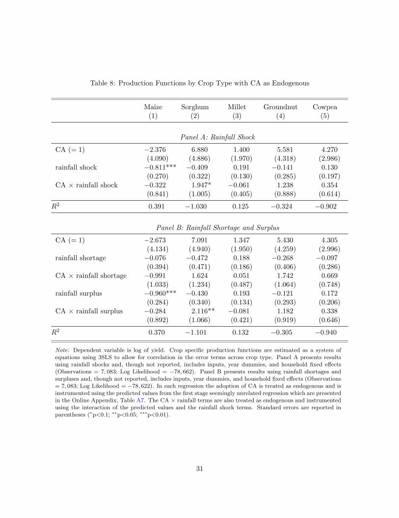
Table 8: Production Functions by Crop Type with CA as Endogenous

Maize Sorghum Millet Groundnut Cowpea(1) (2) (3) (4) (5)

Panel A: Rainfall Shock

CA (= 1) −2.376 6.880 1.400 5.581 4.270(4.090) (4.886) (1.970) (4.318) (2.986)

rainfall shock −0.811*** −0.409 0.191 −0.141 0.130(0.270) (0.322) (0.130) (0.285) (0.197)

CA × rainfall shock −0.322 1.947* −0.061 1.238 0.354(0.841) (1.005) (0.405) (0.888) (0.614)

R2 0.391 −1.030 0.125 −0.324 −0.902

Panel B: Rainfall Shortage and Surplus

CA (= 1) −2.673 7.091 1.347 5.430 4.305(4.134) (4.940) (1.950) (4.259) (2.996)

rainfall shortage −0.076 −0.472 0.188 −0.268 −0.097(0.394) (0.471) (0.186) (0.406) (0.286)

CA × rainfall shortage −0.991 1.624 0.051 1.742 0.669(1.033) (1.234) (0.487) (1.064) (0.748)

rainfall surplus −0.960*** −0.430 0.193 −0.121 0.172(0.284) (0.340) (0.134) (0.293) (0.206)

CA × rainfall surplus −0.284 2.116** −0.081 1.182 0.338(0.892) (1.066) (0.421) (0.919) (0.646)

R2 0.370 −1.101 0.132 −0.305 −0.940

Note: Dependent variable is log of yield. Crop specific production functions are estimated as a system ofequations using 3SLS to allow for correlation in the error terms across crop type. Panel A presents resultsusing rainfall shocks and, though not reported, includes inputs, year dummies, and household fixed effects(Observations = 7, 083; Log Likelihood = −78, 662). Panel B presents results using rainfall shortages andsurpluses and, though not reported, includes inputs, year dummies, and household fixed effects (Observations= 7, 083; Log Likelihood = −78, 622). In each regression the adoption of CA is treated as endogenous and isinstrumented using the predicted values from the first stage seemingly unrelated regression which are presentedin the Online Appendix, Table A7. The CA × rainfall terms are also treated as endogenous and instrumentedusing the interaction of the predicted values and the rainfall shock terms. Standard errors are reported inparentheses (∗p<0.1; ∗∗p<0.05; ∗∗∗p<0.01).

31

Table 9: Production Function with Plot Level Effects

(1) (2)

MaizeCA (= 1) 0.385 1.958

(0.322) (1.892)rainfall shortage −0.388 −1.220**

(0.464) (0.596)CA × rainfall shortage −0.875 3.054**

(0.616) (1.307)rainfall surplus −0.673** −0.617

(0.340) (0.486)CA × rainfall surplus 0.425 1.916**

(0.404) (0.789)Sorghum

CA (= 1) −0.047 3.328(0.647) (2.835)

rainfall shortage −1.389** −1.964***(0.595) (0.566)

CA × rainfall shortage 1.895 3.978**(1.507) (1.793)

rainfall surplus −1.677*** −0.598(0.513) (0.448)

CA × rainfall surplus 1.126 0.287(1.023) (1.193)

MilletCA (= 1) 1.410 7.739

(1.195) (7.046)rainfall shortage −1.079 −1.085

(0.695) (0.711)CA × rainfall shortage −2.383 −3.238

(1.657) (5.807)rainfall surplus −1.319*** −0.572

(0.462) (0.425)CA × rainfall surplus −0.703 0.265

(1.096) (5.322)Groundnut

CA (= 1) −0.580 2.897(0.707) (2.173)

rainfall shortage −1.618*** −1.831***(0.525) (0.611)

CA × rainfall shortage 0.689 0.795(1.038) (1.218)

rainfall surplus −0.208 0.409(0.387) (0.386)

CA × rainfall surplus 0.018 −0.484(1.056) (1.176)

CowpeaCA (= 1) −0.282 0.691

(1.027) (2.235)rainfall shortage −0.150 −2.147*

(1.082) (1.148)CA × rainfall shortage 4.379** 6.127***

(1.865) (2.184)rainfall surplus −1.733* −0.931

(0.902) (0.873)CA × rainfall surplus 2.901* 2.730

(1.682) (2.173)

Plot Controls FE CREObservations 3,344 5,168Kleibergen-Paap LM 9.520***Log Likelihood -6,210 -11,914

Note: Dependent variable is log of yield. Though not re-ported, all specifications include crop-specific inputs andintercept terms, and year dummies. Column (1) restrictsthe sample to plots with more than one observation andwhere CA is either always used or never used. It presentsresults from a plot level fixed effects regression where CA isexogenous. Column (2) restricts the sample to plots withmore than one observation but includes plots where CAstatus changes over time. It presents results from a plotlevel CRE regression where CA is treated as endogenousand is instrumented as described previously. The under-indentification test uses the Kleibergen-Paap LM statistic.All standard errors are clustered at the plot level and arereported in parentheses (∗p<0.1; ∗∗p<0.05; ∗∗∗p<0.01).

32

Figure 1: Location of Surveyed Wards in Zimbabwe

Note: Figure displays the locations of wards in the survey. Shading represents the agro-ecological regions of Zimbabwe.

Regions III, IV, and V are all considered semi-arid and subject to frequent seasonal droughts.

33

Figure 2: Marginal Distributions of Yields by Cultivation Method and Rainfall

Note: Figure displays the kernel density plots of log of yields by either

conservation agriculture (CA) or by traditional cultivation (TC) under

normal and abnormal rainfall.

Figure 3: Average Annual Level of CA Adoption by Crop

Note: Figure displays the average number of plots on which CA tech-

niques are used by crop per year.

34

Figure 4: Historic Seasonal Rainfall by Ward

Note: Figure displays the cumulative rainfall for each cropping season

in each ward for the 15 year period from 1997-2011. A linear trendline

is fitted to the data with a slope of −3.71 which is significantly different

from zero at the 99 percent level. Data comes from the CHIRPS

database (Funk et al., 2015).

Figure 5: Distribution of Seasonal Rainfall by Ward

Note: Figure displays the kernel density of cumulative seasonal rainfall

in each ward for the four year study period (2008-2011). Vertical lines

are drawn at ± half, one, and two standard deviations from the mean,

which is 664mm. Data comes from the CHIRPS database (Funk et al.,

2015).

35

Figure 6: Predicted Returns to CA by Crop

Note: Figure displays the predicted returns to CA averaged over all crops and also by crop. Returns are calculated

using the coefficients from column (3) in Table 7. By crop, we multiple the coefficient on the CA × rainfall shortage

by realized shortages and multiple the coefficient on the CA × rainfall surplus by realized surpluses. We then sum

these values along with the coefficient on the CA term. For the average return we take a weighted average of the

crop specific returns where the weights are the number of observations for each crop in the data. The x-axis marks

the realizations of rainfall surpluses and shortages where shortages are the to left of zero. Dots represent individual

predicted returns where a lower density of dots represents fewer observations, and thus less confidence. Vertical lines

are drawn at ± half, one, and two standard deviations from the mean, which is 0.065.

36

A Appendix For Online Publication: Full Results from Produc-

tion Functions

This appendix contains evidence on the impact of seasonal versus monthly rainfall deviations on

yields. It also contains full specifications and first stage regression results for the models presented in

an abbreviated form in the paper. In all specifications we include controls for crop-specific inputs.

These inputs include logged amounts of basal fertilizer application, top application of fertilizer,

seeds, and land area. Since our primary focus is the impact of CA and rainfall shocks on yields,

we treated these variables as exogenous controls and refrained from reporting the relevant point

estimates in the paper. For those interested in the full specifications, the following tables will be

of interest.

37

Table A1: Production Function with Rainfall Deviations

Maize Sorghum Millet Groundnut Cowpea(1) (2) (3) (4) (5)

Panel A: Deviation in Seasonal Rainfall

Seasonal deviation −0.653*** −1.177*** −1.418*** −0.403* −0.853**(0.195) (0.267) (0.308) (0.214) (0.394)

Panel B: Deviation in Monthly Rainfall

Oct deviation 0.294 −0.298 0.024 0.511*** 0.030(0.193) (0.210) (0.308) (0.197) (0.304)

Nov deviation −0.196* 0.001 −0.070 0.084 −0.070(0.111) (0.175) (0.192) (0.128) (0.237)

Dec deviation −0.186 −0.122 −0.448 0.223* 0.293(0.115) (0.219) (0.305) (0.134) (0.265)

Jan deviation −0.585*** 0.118 −0.273 0.218 0.386*(0.166) (0.174) (0.255) (0.152) (0.233)

Feb deviation −1.103*** −0.361 −0.343 −0.682*** −2.155***(0.215) (0.270) (0.355) (0.256) (0.441)

Mar deviation −1.045** −0.807** −0.605 −0.788*** 0.100(0.186) (0.320) (0.503) (0.241) (0.379)

Apr deviation −0.284*** 0.104 −0.323** −0.116 0.023(0.091) (0.106) (0.135) (0.104) (0.154)

Note: Coefficients are presented in columns based on crop type in order to minimize space. PanelA reports results from a single regression with log yield as the dependent variable and deviations incumulative seasonal rainfall as the variable of interest (Observations = 7, 837; R2 = 0.923). PanelB reports results from a single regression with log yield as the dependent variable and deviations incumulative monthly rainfall as the variables of interest (Observations = 7, 837; R2 = 0.926). Thoughnot reported, both specifications include crop-specific CA adoption term, crop-specific inputs, crop-specific intercept terms, year dummies, and household fixed effects. Standard errors clustered byhousehold and crop are reported in parentheses (∗p<0.1; ∗∗p<0.05; ∗∗∗p<0.01).

38

Table A2: Production Function with CA as Exogenous

(1) (2) (3) (4)

MaizeCA (= 1) 0.645*** 0.577*** 0.198 0.197

(0.083) (0.081) (0.139) (0.136)rainfall shock −0.690*** −0.943***

(0.217) (0.230)CA × rainfall shock 0.958*** 0.776***

(0.251) (0.238)ln(basal) 0.117*** 0.072*** 0.119*** 0.078***

(0.025) (0.024) (0.025) (0.024)ln(top) 0.324*** 0.276*** 0.314*** 0.267***

(0.028) (0.026) (0.028) (0.026)ln(seed) 0.286*** 0.267*** 0.273*** 0.254***

(0.078) (0.073) (0.078) (0.073)ln(area) −0.514*** −0.536*** −0.506*** −0.525***

(0.067) (0.067) (0.066) (0.066)Sorghum

CA (= 1) −0.033 −0.067 −0.783*** −0.576**(0.181) (0.191) (0.272) (0.286)

rainfall shock −1.305*** −1.467***(0.301) (0.313)

CA × rainfall shock 1.572*** 1.060**(0.464) (0.501)

ln(basal) 0.029 −0.001 0.031 0.006(0.085) (0.068) (0.088) (0.068)

ln(top) 0.125* 0.145** 0.122* 0.138**(0.066) (0.059) (0.065) (0.058)

ln(seed) 0.390*** 0.407*** 0.390*** 0.406***(0.109) (0.111) (0.108) (0.110)

ln(area) −0.601*** −0.620*** −0.572*** −0.590***(0.083) (0.091) (0.083) (0.091)

MilletCA (= 1) −0.167 0.180 −1.066 −0.731

(0.357) (0.374) (0.711) (0.733)rainfall shock −1.094*** −1.563***

(0.303) (0.316)CA × rainfall shock 1.596* 1.637

(0.945) (1.165)ln(basal) 0.209* 0.143 0.170 0.097

(0.107) (0.130) (0.104) (0.130)ln(top) −0.260** −0.134 −0.242** −0.114

(0.121) (0.126) (0.120) (0.121)ln(seed) 0.153 0.203 0.190 0.239*

(0.159) (0.144) (0.158) (0.140)ln(area) −0.464*** −0.594*** −0.474*** −0.604***

(0.130) (0.128) (0.128) (0.124)Groundnut

CA (= 1) 0.218 0.286** −0.575** −0.029(0.143) (0.144) (0.288) (0.281)

rainfall shock −0.462** −0.538**(0.208) (0.228)

CA × rainfall shock 1.419*** 0.553(0.488) (0.454)

ln(basal) 0.067 −0.026 0.074 −0.026(0.071) (0.062) (0.069) (0.062)

ln(top) −0.068 −0.019 −0.028 −0.004(0.070) (0.060) (0.068) (0.060)

ln(seed) 0.483*** 0.396*** 0.481*** 0.392***(0.088) (0.083) (0.087) (0.083)

ln(area) −0.523*** −0.623*** −0.518*** −0.612***(0.079) (0.073) (0.079) (0.074)

Continued on Next Page. . .

39

Table A2 – Continued

(1) (2) (3) (4)

CowpeaCA (= 1) −0.059 0.232 −0.983** −0.429

(0.242) (0.252) (0.455) (0.447)rainfall shock −1.058** −1.216***

(0.444) (0.435)CA × rainfall shock 1.924** 1.321

(0.895) (0.874)ln(basal) 0.336*** 0.129 0.327*** 0.129

(0.106) (0.088) (0.105) (0.088)ln(top) −0.164 −0.137 −0.147 −0.125

(0.109) (0.097) (0.110) (0.098)ln(seed) 0.370*** 0.412*** 0.389*** 0.422***

(0.138) (0.139) (0.139) (0.139)ln(area) −0.588*** −0.716*** −0.596*** −0.720***

(0.102) (0.106) (0.103) (0.108)

Household FE No Yes No YesObservations 7,837 7,837 7,837 7,837R2 0.898 0.922 0.899 0.923

Note: Dependent variable is log of yield. All specifications include crop-specific intercept termsand year dummies. Column (1) excludes rainfall variables as well as household fixed effects.Column (2) excludes rainfall variables but includes household fixed effects. Column (3) includesthe rainfall shock and its interaction with CA but excludes household fixed effects. Column (4)includes both the rainfall shock, its interaction with CA, and household fixed effects. Standarderrors clustered by household and crop are reported in parentheses (∗p<0.1; ∗∗p<0.05; ∗∗∗p<0.01).

40

Table A3: Production Function with CA as Endogenous

(1) (2) (3) (4)

MaizeCA (= 1) 7.233* −1.289 6.659 −2.413*

(4.255) (1.286) (5.359) (1.378)rainfall shock −0.440 −1.656***

(0.791) (0.377)CA × rainfall shock 2.009 2.690***

(1.470) (0.736)ln(basal) −0.270 0.174** −0.281 0.184**

(0.247) (0.078) (0.285) (0.074)ln(top) 0.013 0.375*** −0.022 0.340***

(0.210) (0.073) (0.229) (0.065)ln(seed) 1.015** 0.078 1.052* 0.089

(0.475) (0.162) (0.543) (0.153)ln(area) −0.211 −0.636*** −0.180 −0.601***

(0.232) (0.101) (0.253) (0.093)Sorghum

CA (= 1) 10.882** 0.202 11.961* 0.185(5.383) (1.678) (6.868) (1.862)

rainfall shock −1.155** −1.494***(0.488) (0.358)

CA × rainfall shock −0.437 0.806(1.987) (0.955)

ln(basal) −0.487* −0.009 −0.491 −0.018(0.288) (0.119) (0.317) (0.108)

ln(top) −1.654* 0.096 −1.811* 0.032(0.887) (0.258) (1.044) (0.247)

ln(seed) 0.368** 0.388*** 0.376* 0.396***(0.184) (0.106) (0.193) (0.106)

ln(area) 0.421 −0.572*** 0.515 −0.509***(0.513) (0.181) (0.591) (0.169)

MilletCA (= 1) 16.373 −1.926 21.906 −1.133

(11.625) (3.323) (20.303) (3.897)rainfall shock −0.422 −1.693***

(0.702) (0.337)CA × rainfall shock −4.889 2.449

(12.602) (2.250)ln(basal) −0.831 0.274 −0.938 0.090

(0.874) (0.224) (0.976) (0.199)ln(top) −2.562 0.173 −3.006 −0.103

(1.737) (0.493) (2.261) (0.471)ln(seed) −0.617 0.278 −0.761 0.234

(0.657) (0.198) (0.864) (0.188)ln(area) 1.513 −0.854** 1.872 −0.603

(1.475) (0.408) (1.891) (0.392)Groundnut

CA (= 1) 8.800** 0.586 8.726* 0.257(3.939) (1.321) (4.938) (1.554)

rainfall shock −1.122*** −0.893***(0.394) (0.269)

CA × rainfall shock 1.492 1.140(1.733) (0.892)

ln(basal) −0.653* −0.064 −0.690 −0.087(0.371) (0.121) (0.422) (0.115)

ln(top) −1.131** −0.055 −1.207* −0.065(0.518) (0.166) (0.620) (0.173)

ln(seed) 0.720*** 0.477*** 0.745*** 0.468***(0.204) (0.089) (0.224) (0.091)

ln(area) 0.035 −0.614*** 0.077 −0.580***(0.298) (0.115) (0.336) (0.107)

Continued on Next Page. . .

41

Table A3 – Continued

(1) (2) (3) (4)

CowpeaCA (= 1) 5.985* −0.069 4.840 −1.017

(3.256) (1.231) (4.068) (1.439)rainfall shock −1.004 −1.659***

(0.720) (0.471)CA × rainfall shock 2.962 2.481*

(2.067) (1.413)ln(basal) 0.148 0.147 0.124 0.133

(0.179) (0.100) (0.185) (0.098)ln(top) −1.154** −0.092 −1.158* −0.104

(0.563) (0.198) (0.634) (0.193)ln(seed) −0.036 0.432*** −0.020 0.448***

(0.281) (0.147) (0.311) (0.148)ln(area) −0.029 −0.747*** −0.013 −0.727***

(0.321) (0.152) (0.362) (0.150)

Household FE No Yes No YesKleibergen-Paap LM 4.875** 21.38*** 3.865** 25.17***Observations 7,837 7,837 7,837 7,837Log Likelihood -21,406 -16,587 -21,798 -16,527

Note: Dependent variable is log of yield. All specifications include crop-specific intercept terms andyear dummies. In each regression the adoption of CA is treated as endogenous and is instrumentedwith the Inverse Mills Ratio (IMR) calculated from the predicted values of the first stage regressionsreported in Table 5. The CA × rainfall shock term is also treated as endogenous and instrumentedusing the interaction of the IMR and the rainfall shock term. The underindentification test uses theKleibergen-Paap LM statistic. Column (1) excludes rainfall variables as well as household fixed effects.Column (2) excludes rainfall variables but includes household fixed effects. Column (3) includes therainfall shock and its interaction with CA but excludes household fixed effects. Column (4) includesboth the rainfall shock, its interaction with CA, and household fixed effects. Standard errors clusteredby household and crop are reported in parentheses (∗p<0.1; ∗∗p<0.05; ∗∗∗p<0.01).

Table A4: First Stage IV Probit with Rain Shortage or Surplus

(1) (2) (3)

Num HH in ward with NGO support 0.010*** 0.009*** 0.009***(0.001) (0.001) (0.001)

Household CRE Yes Yes YesObservations 7,837 7,837 7,837Log Likelihood -3,226 -3,223 -3,217

Note: Regressions are probits that include the IV, crop-specific inputs and intercept terms, and yeardummies. The instrument is the number of households in the ward that receive NGO support. Column(1) includes a rainfall shortage, column (2) includes a rainfall surplus, and column (3) includes both arainfall shortage and a rainfall surplus. Standard errors clustered by household and crop are reported inparentheses (∗p<0.1; ∗∗p<0.05; ∗∗∗p<0.01).

42

Table A5: Production Function with Rain Shortage or Surplus

(1) (2) (3)

MaizeCA (= 1) 0.470 −2.052 −1.145

(1.590) (1.656) (1.802)rainfall shortage 0.293 −0.918*

(0.412) (0.519)CA × rainfall shortage −0.099 1.984*

(0.752) (1.049)rainfall surplus −1.683*** −1.884***

(0.306) (0.386)CA × rainfall surplus 2.147*** 2.964***

(0.493) (0.701)ln(basal) 0.074 0.204** 0.116

(0.091) (0.099) (0.097)ln(top) 0.279*** 0.366*** 0.271***

(0.084) (0.091) (0.085)ln(seed) 0.262 0.077 0.222

(0.186) (0.198) (0.192)ln(area) −0.535*** −0.621*** −0.529***

(0.113) (0.115) (0.111)Sorghum

CA (= 1) 0.197 −0.574 −0.021(1.652) (2.367) (2.080)

rainfall shortage −1.144*** −1.736***(0.391) (0.455)

CA × rainfall shortage 3.139** 2.749**(1.305) (1.332)

rainfall surplus −0.465 −1.166***(0.356) (0.390)

CA × rainfall surplus −0.880 0.176(1.111) (1.067)

ln(basal) −0.037 0.077 −0.006(0.120) (0.124) (0.116)

ln(top) 0.011 0.248 0.040(0.275) (0.327) (0.293)

ln(seed) 0.398*** 0.398*** 0.406***(0.107) (0.106) (0.106)

ln(area) −0.536*** −0.680*** −0.540***(0.183) (0.200) (0.184)

MilletCA (= 1) −0.418 −1.914 −0.163

(2.826) (3.570) (3.455)rainfall shortage −0.599 −1.637**

(0.592) (0.638)CA × rainfall shortage −0.005 1.222

(1.401) (2.299)rainfall surplus −1.184*** −1.619***

(0.376) (0.328)CA × rainfall surplus 2.168 2.188

(1.509) (2.242)ln(basal) 0.163 0.168 0.033

(0.203) (0.198) (0.185)ln(top) −0.043 0.098 −0.196

(0.429) (0.483) (0.427)ln(seed) 0.220 0.263 0.198

(0.188) (0.186) (0.179)ln(area) −0.670* −0.737* −0.510

(0.361) (0.387) (0.351)

Continued on Next Page. . .

43

Table A5 – Continued

(1) (2) (3)

GroundnutCA (= 1) 0.997 −0.957 0.390

(1.298) (1.764) (1.769)rainfall shortage −1.121*** −1.186***

(0.320) (0.334)CA × rainfall shortage 0.177 0.136

(0.723) (1.033)rainfall surplus 0.111 −0.081

(0.324) (0.310)CA × rainfall surplus −0.147 −0.537

(0.951) (1.120)ln(basal) −0.083 0.058 −0.033

(0.117) (0.140) (0.121)ln(top) −0.129 0.142 −0.035

(0.167) (0.196) (0.190)ln(seed) 0.472*** 0.446*** 0.456***

(0.091) (0.083) (0.089)ln(area) −0.600*** −0.721*** −0.653***

(0.113) (0.110) (0.104)Cowpea

CA (= 1) 0.232 −0.022 −0.411(1.237) (1.559) (1.581)

rainfall shortage −0.507 −1.434***(0.479) (0.546)

CA × rainfall shortage 3.314*** 4.067***(1.047) (1.331)

rainfall surplus −1.170** −1.558***(0.477) (0.547)

CA × rainfall surplus −0.329 1.463(1.307) (1.668)

ln(basal) 0.058 0.166 0.076(0.101) (0.111) (0.104)

ln(top) −0.197 −0.099 −0.182(0.199) (0.218) (0.207)

ln(seed) 0.431*** 0.440*** 0.442***(0.149) (0.150) (0.152)

ln(area) −0.681*** −0.760*** −0.690***(0.154) (0.163) (0.157)

Household FE Yes Yes YesObservations 7,837 7,837 7,837Kleibergen-Paap LM 18.32*** 15.75*** 17.67***Log Likelihood -16,282 -16,607 -16,272

Note: Dependent variable is log of yield. All specifications include crop-specificintercept terms and year dummies. In each regression the adoption of CA istreated as endogenous and is instrumented with the Inverse Mills Ratio (IMR)calculated from the predicted values of first stage regressions which are presentedin Table A4. The CA × rainfall shortage and CA × rainfall surplus terms arealso treated as endogenous and instrumented using the interaction of the IMRand the rainfall terms. The underindentification test uses the Kleibergen-PaapLM statistic. Column (1) includes a rainfall shortage and its interaction with theinstrumented CA term. Column (2) includes a rainfall surplus and its interactionwith the instrumented CA term. Column (3) includes both a rainfall shortage anda rainfall surplus and their interactions with the instrumented CA term. Stan-dard errors clustered by household and crop are reported in parentheses (∗p<0.1;∗∗p<0.05; ∗∗∗p<0.01).

44

Table A6: Production Function with Alternative Rainfall Measures

(1) (2)

MaizeCA (= 1) −1.849 −3.143**

(1.322) (1.446)rainfall shock −0.975*** −0.843***

(0.322) (0.282)CA × rainfall shock 2.120*** 2.156***

(0.530) (0.526)Sorghum

CA (= 1) −0.131 −1.167(1.693) (1.853)

rainfall shock −0.664** −0.718**(0.301) (0.292)

CA × rainfall shock 0.711 0.408(0.617) (0.617)

MilletCA (= 1) −1.161 −2.725

(2.889) (3.139)rainfall shock −0.534* −0.724**

(0.307) (0.307)CA × rainfall shock −0.848 −0.507

(2.074) (1.413)Groundnut

CA (= 1) 0.335 −0.847(1.353) (1.433)

rainfall shock −0.367 −0.432**(0.249) (0.218)

CA × rainfall shock 0.809 1.152**(0.612) (0.574)

CowpeaCA (= 1) −0.172 −1.204

(1.248) (1.385)rainfall shock −0.744* −1.199***

(0.431) (0.418)CA × rainfall shock 0.044 1.803*

(1.293) (1.081)

Household FE Yes YesKleibergen-Paap rk LM statistic 23.04*** 20.35***Observations 7,837 7,837Log Likelihood -16,661 -17,022

Note: Dependent variable is log of yield. All specifications includecrop-specific intercept terms and year dummies. In each regressionthe adoption of CA is treated as endogenous and is instrumentedas previously discussed. Column (1) replaces any deviation in rain-fall that is with ± one standard deviation with a zero. Thus, anyrealized value that is 0.202 ≤ R jt ≤ 0.748 is set to zero. Column(2) replaces any deviation in rainfall that is with ± one half of astandard deviation with a zero. Thus, any realized value that is0.338 ≤ R jt ≤ 0.612 is set to zero. Standard errors clustered byhousehold and crop are reported in parentheses (∗p<0.1; ∗∗p<0.05;∗∗∗p<0.01). 45

Table A7: First Stage IV by Crop Type

Maize Sorghum Millet Groundnut Cowpea(1) (2) (3) (4) (5)

Panel A: Rainfall Shock

Num HH with NGO support −0.001** 0.001*** −0.000 0.001** 0.001***(0.001) (0.000) (0.000) (0.000) (0.000)

R2 0.327 0.167 0.112 0.135 0.139

Panel B: Rainfall Shortage and Surplus

Num HH with NGO support −0.001** 0.001*** −0.000 0.001** 0.001***(0.001) (0.000) (0.000) (0.000) (0.000)

R2 0.327 0.168 0.112 0.136 0.139

Note: Panel A reports results from a first stage seemingly unrelated regression with CA adoption as the dependentvariable and includes the IV, rainfall shock, inputs, year dummies, and household fixed effects (Observations= 7, 837; Log Likelihood = 13, 700). Panel B reports results from a first stage seemingly unrelated regression withCA adoption as the dependent variable and includes the IV, rainfall shortages and surplus, inputs, year dummies,and household fixed effects (Observations = 7, 837; Log Likelihood = 13, 713). Standard errors are reported inparentheses (∗p<0.1; ∗∗p<0.05; ∗∗∗p<0.01).

Table A8: First Stage IV Tobit with Rain Shortage and Surplus

(1) (2)

Num HH in ward with NGO support 0.005** 0.007***(0.002) (0.001)

Household Control FE CREObservations 7,837 7,837Log Likelihood -4,483 -5,060

Note: Regressions are first stage Tobits with CA adoption as the dependent vari-able and includes the IV, rainfall shortages and surpluses, crop-specific inputs andintercept terms, and year dummies. The instrument is the number of households inthe ward that receive NGO support. Column (1) includes household fixed effects,column (2) includes household correlated random effects. Standard errors clusteredby household and crop are reported in parentheses (∗p<0.1; ∗∗p<0.05; ∗∗∗p<0.01).

46

Table A9: Production Function using First Stage Tobit

(1) (2)

MaizeCA (= 1) −0.037 −0.998

(0.472) (0.809)rainfall shortage −0.358 −0.710

(0.368) (0.450)CA × rainfall shortage 0.394 1.226

(0.695) (0.954)rainfall surplus −1.471*** −1.823***

(0.321) (0.334)CA × rainfall surplus 1.842*** 2.751***

(0.544) (0.631)Sorghum

CA (= 1) 0.154 −0.303(0.774) (1.027)

rainfall shortage −1.753*** −1.935***(0.423) (0.444)

CA × rainfall shortage 2.725** 3.674***(1.105) (1.229)

rainfall surplus −1.273*** −1.456***(0.363) (0.364)

CA × rainfall surplus 0.512 1.103(0.762) (0.830)

MilletCA (= 1) −1.580 −1.291

(1.716) (1.755)rainfall shortage −1.798*** −1.763***

(0.612) (0.618)CA × rainfall shortage 2.814 2.713

(2.495) (2.543)rainfall surplus −1.574*** −1.723***

(0.303) (0.297)CA × rainfall surplus 2.698 3.515*

(1.799) (2.008)Groundnut

CA (= 1) 0.306 0.385(0.541) (0.675)

rainfall shortage −1.208*** −1.257***(0.320) (0.322)

CA × rainfall shortage 0.362 0.585(0.720) (0.807)

rainfall surplus −0.110 −0.113(0.250) (0.251)

CA × rainfall surplus −0.207 −0.436(0.597) (0.677)

CowpeaCA (= 1) −1.118 −0.931

(0.768) (1.064)rainfall shortage −1.533*** −1.552***

(0.532) (0.554)CA × rainfall shortage 4.461*** 4.488***

(1.167) (1.387)rainfall surplus −1.835*** −1.714***

(0.513) (0.533)CA × rainfall surplus 2.785** 2.148

(1.406) (1.718)

Household FE Yes YesObservations 7,837 7,837Kleibergen-Paap LM 256.2*** 164.8***Log Likelihood -16,223 -16,273

Note: Dependent variable is log of yield. Though notreported, all specifications include crop-specific inputs andintercept terms, and year dummies. Column (1) uses thepredicted value and the Inverse Mills Ratio from the firststage Tobit with household fixed effects as presented incolumn (1) of Table A8. Column (2) uses the predictedvalue and the Inverse Mills Ratio from the first stage Tobitwith household correlated random effects as presented incolumn (2) of Table A8. The underindentification testuses the Kleibergen-Paap LM statistic. All standard errorsare clustered by household and crop and are reported inparentheses (∗p<0.1; ∗∗p<0.05; ∗∗∗p<0.01).

47