consequences of fault currents contributed by distributed ......fault calculations in power systems...
TRANSCRIPT

Consequences of Fault CurrentsContributed by Distributed Generation
Intermediate Project Report
Power Systems Engineering Research Center
A National Science FoundationIndustry/University Cooperative Research Center
since 1996
PSERC

Power Systems Engineering Research Center
Consequences of Fault Currents Contributed by Distributed Generation
Intermediate Report for the Project “New Implications of Power System Fault Current Limits”
N. Nimpitiwan G. T. Heydt
Arizona State University
PSERC Publication 04-34
November 2004

Information about this project For information about this project contact: G. T. Heydt Regents’ Professor Arizona State University PO Box 875706 Tempe, AZ 85259-5706 Tel: 480-965-8307 Fax: 480-965-0745 Email: [email protected] Power Systems Engineering Research Center This is a project report from the Power Systems Engineering Research Center (PSERC). PSERC is a multi-university Center conducting research on challenges facing a restruc-turing electric power industry and educating the next generation of power engineers. More information about PSERC can be found at the Center’s website: http://www.pserc.wisc.edu. For additional information, contact: Power Systems Engineering Research Center Cornell University 428 Phillips Hall Ithaca, New York 14853 Phone: 607-255-5601 Fax: 607-255-8871 Notice Concerning Copyright Material PSERC members are given permission to copy without fee all or part of this publication for internal use if appropriate attribution is given to this document as the source material. This report is available for downloading from the PSERC website.
© 2004 Arizona State University. All rights reserved.

Acknowledgements
The Power Systems Engineering Research Center sponsored the research project titled “New Implications of Power System Fault Current Limits.” This project is under-way at the time of writing (November, 2004). This report is an intermediate report of progress at Arizona State University. We express our appreciation for the support provided by PSERC’s industrial mem-bers and by the National Science Foundation under grant NSF EEC-0001880 received under the Industry / University Cooperative Research Center program. The authors thank all PSERC members for their technical advice on this project. Special thanks go to Dr. R. Thallam and Messrs. J. Blevins and A. B. Cummings of Salt River Project for their technical input. We are also indebted to Professors A. Bose and A. P. S. Meliopoulos of Washington State University and Georgia Tech respectively for their work on this project.

Executive Summary This report concerns fault currents in systems with distributed generation. The main concept described is that fault current throughout power systems is likely to in-crease when distributed generation is installed. The nature of the increase is described in some detail, mainly using the Zbus method of calculation. IEEE standards are used to ap-ply correction factors. The requirements of IEEE Standard 1547 are applied as well – this is a standard for distributed generation use.
Fault calculations in power systems are used to determine the interrupting capa-bility of circuit breakers. The calculation of fault current at the system buses is done by applying the system Zbus matrix. The effects of merchant plants, such as Independent Power Producers, are not taken into consideration in the classical fault current calcula-tion. New developments in deregulation have brought new generation sources to the sys-tem. The appearance of DGs is a cause of increasing fault currents that has not previ-ously been envisioned. This report presents a modification of the conventional fault cur-rent calculation in the case of addition of DGs. Many consequences arise from increasing of the fault currents, for instance the change of coordination of protective devices, nui-sance trips, safety degradation, and the requirement to change recloser and protective re-lay settings. These consequences result in the cost of equipment upgrades not only at the DG sites but also other system sites.
Due to installing new DGs, six main factors that affect the severity of the increase of three phase fault current at each buses are:
• the number and size of DGs • the operation of the AVR • the impedance of DGs • the location of DGs • the type of DGs • circuit breaker configuration.
In the report, an index called the average change of fault current or “ACF” is pro-posed. The ACF can be used to indicate the severity of the change of fault current due to installing new DGs. Chapter 4 proposes the least squares method to approximate the ACF for a given system. By this proposed technique, the pre-fault voltages and the fault current calculation may not be needed in the preliminary design stage. Note that in the preliminary design stage there may be a very large number of calculations, and the ACF concept can speed up the analysis. The only required input of the least squares method is the impedance of a new DG and its location. The advantages of this technique are: • faster calculation due to the fact that load flow solution and fault calculations are not
required • contribution of the increase of fault current is indicated at each location of 12 kV bus
in the primary distribution system. By this concept, each new DG is treated in an equitable way. The ACF concept is offered as a rapid way to assess fault currents when DGs are deployed in any number, anywhere in the system.
• The main disadvantage of the ACF method relates to accuracy. That is, even though the estimator may have been constructed for a large number of sample cases, there is no guarantee that the ACF calculation will be accurate.
ii

Table of Contents
Acknowledgements ............................................................................................................. iExecutive Summary ........................................................................................................... iiTable of Contents .............................................................................................................. iiiTable of Figures ................................................................................................................ ivTable of Tables ...................................................................................................................vNomenclature .................................................................................................................... vi1. Introduction................................................................................................................. 1
1.1 Motivation............................................................................................................... 1 1.2 Objectives ............................................................................................................... 2 1.3 Literature review: distributed generation................................................................ 2 1.4 IEEE Standards ....................................................................................................... 8 1.5 Literature review: systems and hardware ............................................................. 12
2. The Theory of Fault Analysis ................................................................................... 15 2.1 The analysis of power system faults ..................................................................... 15 2.2 Modification of traditional algorithms of fault current calculation ...................... 15 2.3 An illustrative example ......................................................................................... 19
3. Factors that Affect the Severity of Fault Currents: Illustrative Case Studies ........... 21 3.1 Introduction........................................................................................................... 21 3.2 Fault analysis for the Thunderstone system.......................................................... 22 3.3 Conclusions........................................................................................................... 28
4. Fault Calculation by the Least Squares Method ....................................................... 32 4.1 Introduction........................................................................................................... 32 4.2 A least squares estimate of ACF........................................................................... 32 4.3 Application of the least squares method to the Thunderstone system, Case 4.1 .. 35 4.4 Confidence interval on the least squares estimator coefficient............................. 39 4.5 Confidence interval estimation of the mean response of ACF ............................. 40 4.6 Circuit breaker sizing............................................................................................ 43 4.7 Allocation of the responsibility for the system upgrades to the owner of DGs.... 45 4.8 Conclusions........................................................................................................... 49
5. Implication of Fault Current Increase on Optimal Power Flow ............................... 51 5.1 Implications of fault current in an OPF ................................................................ 51 5.2 An illustration of operating implications of fault current ..................................... 51 5.3 Production cost of the merchant plant under the fault current limitation constraint
57 5.4 Conclusions........................................................................................................... 57
6. Conclusions and Recommendations ......................................................................... 58 6.1 Conclusions........................................................................................................... 58 6.2 Potential new research areas ................................................................................. 59
References......................................................................................................................... 61 Appendix A....................................................................................................................... 65 Appendix B ....................................................................................................................... 68
iii

Table of Figures Figure Page 1.1 Reciprocating engines and gas turbines less than 20 MW …………. 3 1.2 Electrode reactions and charges flow for an acid electrolyte fuel
cell……………………………………………………………………. 4 1.3 The reach of a protective relay for a small sample distribution system
with DGs……………………………………………………………... 7 1.4 Time-current characteristic of the fuse in the sample system………... 8 1.5 Three phase fault multiplying factors………………………………... 11 1.6 Line-to-ground fault multiplying factors…………………………….. 11 2.1 New DG added to bus k through its internal impedance creating a new
bus p…………………………………………………….. 15 2.2 Fault occurs at bus j in the system including the new
DG…………………………………………………………….. 17 2.3 A 4-bus system with new DGs at bus 3 and 4…………... 19 3.1 Thunderstone 69 kV transmission system……………….. 23 3.2 The change of fault current of the system after installing a new DG at
Cameron2, Case 3.1……………………...…. 25 3.3 The change of fault current of the system after installing a new DG at
Cameron2 and Signal13, Case 3.1…………………………………… 26 3.4 The change of fault current of the system after installing a new DG at
Cameron2, Signal13 and Seaton2, Case 3.1…………………………. 27 3.5 The change of fault current of the system after installing a new DG at
Cameron2, Signal13, Seaton2 and Sage3, Case 3.1 29 3.6 Thunderstone system with new DGs at Seaton, Cameron2, Signal3 and
Sage3, Case 3.2………………………………………………….. 30 3.7 Increasing of fault current as a result of turning AVR control on/off,
Case 3.2………………………………………………………………. 31 3.8 The increasing of fault current dues to varying the reactance of DGs,
Case 3.3………………………………………………………………. 31 4.1 System diagram of the least square estimator………………………... 32 4.2 Residual of the least squares estimator, Case 4.1……………………. 38 4.3 Plot of the bus ACF and the total ACF, Case 4.1……………………. 39 4.4 Comparison between the full fault calculation and the least squares es-
timator model, Case 4.1……………………………………………. 41 4.5 E/X method with adjustment for the AC and DC increment………… 44 5.1 Incremental cost function of the merchant plants for Case 5.1 and 5.2 52 5.2 Economic dispatch for all units (without fI condition): Case 5.1...... 54
5.3 Incremental cost curve (without fI condition): Case 5.1…………... 54
5.4 Economic dispatch for all units (with fI condition) when Unit 2 and 3 are in service, Case 5.2……………………………..……………… 56
5.5 Incremental cost curve (with fI condition), Case 5.2……………… 56
iv
Table of Tables
Table Page 1.1 Approximate price of DG per kilowatt …………………………… 4 1.2 Data for different type of fuel cells ……………………………….. 5 1.3 Required clearing times for DGs higher than 30 kW, from IEEE
1547 ………………………………………………………………... 9
2.1 Summary of calculation for the simple 4-bus system shown in Fig-ure 2.3 ………………………………………………………………
20
3.1 Results of installing new DGs at various number and locations in the Thunderstone system Case 3.1 ……………………………………..
24
4.1 Dimensions of several quantities used in the least squares estimation of ACF ……………………………………………………………..
34
4.2 List of the buses with new DG in Case 4.1 ………………………… 35 4.3 Norm of residual of Case 4.1………………………………... 36 4.4 Confidence interval of the coefficient of the ACF model, Case 4.1 ... 42 4.5 Percent confidence and their confidence intervals for the mean re-
sponse of the ACF of the Thunderstone system, Case 4.1 …………. 43
4.6 Fault current calculation for Thunderstone system, Case 4.2 ……… 46 4.7 Preferred ratings for CBs in Thunderstone system before installing
DGs, Case 4.2 …………………………………………. 47
4.8 Preferred ratings for CBs in Thunderstone system after installing DGs, Case 4.2 ………………………………………….
48
4.9 Cost for upgrades the system due to installing new DGs, Case 4.2 49 4.10 The average change of fault current (ACF) due to installing new DG
in to the Thunderstone system, Case 4.1 …………………. 50
5.1 Merchant plant data: Cases 5.1 and 5.2 ……………………………. 52 5.2 Limitation of the system operation due to the increase of fault cur-
rent, Case 5.2 ……………………………………………………….. 55
5.3 Operating cost of serving the demand: Case 5.2 …………………… 57 6.1 Summary of the topics in this report ………………………………. 59 A.1 Transmission line parameter for Thunderstone system ……………. 65 A.2 Load bus data ………………………………………………………. 66 A.3 Substation transformer (230/69 kV) at Thunderstone substation 66 A.4 Distribution transformers …………………………………………… 67 B.1 Summary of the case studies ………………………………………. 68
v

Nomenclature
AC Alternating current ACF Average change of fault current ACF(bus) Bus ACF AVR Automatic voltage regulator CAAA Clean air act amendments CB Electric circuit breaker CHP Combined heat and power CIGRE International Council on Large Electricity Systems DC Direct current DG Distributed generation DGimp Impedance of distributed generator DOE Department of Energy DR Distributed resource E Pre-fault voltage EA Evolutionary algorithm ECED Environmentally constrained economic dispatch ED Economic dispatch EIC Equal incremental cost method EMI Electromagnetic interference EP Evolutionary programming EPRI Electric Power Research Institute EPS Electric power system ES Evolutionary strategy E/X Ratio of system voltage and equivalent reactance fj Function applied in the least squares estimator F Relationship matrix F+ Pseudoinverse of the relationship matrix FCL Fault current limiter GA Genetic algorithm GP Genetic programming HGA Hierarchical genetic algorithm i Complex number 1− IC Current interrupting capability IPP Independent power producer Ifj Fault current at bus j If,n Fault current at bus n before installing new DG IfDG,n Fault current at bus n after installing new DGs Ip Injected current at bus p j Complex number 1− k Order of the function applied in the least squares estimator
qrλ Primitive line impedance from bus q to bus r m Number of the bus with DG MM Minimum melting time of fuse
vi

MTG Microturbine generators MCFC Molten carbonate fuel cells n Number of all historical data nDG Number of bus with DG nbus Total buses in the system NUG Non-utility generator OPF Optimal power flow p Number of the coefficient of the least squares estimator PAFC Phosphoric acid fuel cells PCC Point of common coupling PEM Proton exchange membrane PDG Critical power rating of distributed generation PV Photovoltaic q Number of the historical data (cases) r Residual of the least squares estimator RRRV Rate of rise recovery voltage SFCL Superconductor fault current limiter SOFC Solid oxide fuel cell SSRes Residual or error sum of squares SRP Salt River Project
pnt −,2/α Value from t-distribution TC Total clearing time of fuse UF Fraction of the total cost paid by utility company
0iV Voltage at bus i before installing DG
Vf Pre-fault voltage Vj Voltage at bus j during fault w Coefficient vector w Estimate value of w X0 Zero sequence equivalent reactance of the system X1 Positive sequence equivalent reactance of the system X System reactance X/R Ratio of system equivalent reactance to system equivalent re-
sistance y Output vector of the least square estimation technique Zbus Bus impedance matrix
+busZ Positive sequence bus impedance matrix −busZ Negative sequence bus impedance matrix 0busZ Zero sequence bus impedance matrix
zgen Generator transient impedance )(
,
b
DGz λ Transient impedance of DG at bus λ case b Zorig Bus impedance matrix of original system zf Fault impedance Zij,orig Diagonal element of bus impedance matrix of the system be-
fore installing new DG
vii

Zij,new Diagonal element of bus impedance matrix of the system after installing new DG
∆ fI Change of fault current due to installing new DGs
∆ V Change in voltage σr
2 Variance of residual 2
rσ Estimation of variance of residual Ω Off line analyzed cases
viii

1. Introduction
1.1 Motivation Deregulation, utility restructuring, technology evolution, environmental policies and in-
creasing electric demand are stimuli for deploying new distributed generation (DG). According to the US Department of Energy (DOE), DG is defined as [5] “the modular electric generation or storage located near the point of use. Distributed generation systems include biomass-based generators, combustion turbines, thermal solar power and photovoltaic systems, fuel cells, wind turbines, microturbines, engines/generator sets and storage and control technologies. Distributed resources can either be grid connected or independent of the grid. Those connected to the grid are typically interfaced at the distribution system”. According to the IEEE Standard 1547-2003, DG is defined as “Electric generation facilities connected to an area Electric Power System (EPS) operator through a Point of Common Coupling (PCC); a subset of Distributed Resource (DR)” [ 6 ]. Reduction of investment in transmission and distribution system upgrades and fast installation are the major benefits to the power utilities. Many applications, such as upgrading the reliability of the power supply, peak shaving, grid support and combined heat and power (CHP), are the major benefits to distributed generation owners.
However, the appearance of co-generation, DG, and unconventional generation may re-sult in unwanted (and often unexpected) consequences. This report focuses on one such un-wanted consequence: increased fault current. In this report focus is given to operation during faulted conditions. Circuit breaker capability and configuration of protective relays that were previously designed for the system without DGs may not safely manage faults. There may be some operating and planning conditions that are imposed by the fault current interrupting capa-bility of the existing circuit breakers and the protective relay configurations. These situations can result in the safety degradation of the electric power system. At present, there is a very low penetration of DG in the United States (about 18 % of the total installed generation capacity is DG according to [21]). However, many indicators imply that DG penetration is increasing. The cited fault current concerns are expected to occur at higher levels of DG penetration. Also, lo-cally DG penetration could be high in some circumstances. The identification and alleviation of degraded operation of power systems during fault conditions is the main objective of this work.
Assessment of the ability of power systems to manage the increase of fault currents due to DGs should be investigated. Fault currents in power systems determine the ratings of the cir-cuit interruption devices and the settings of power system protective relays. Once the circuit breakers are in place and relay settings have been implemented, there may be some operating and planning implications imposed by the changing fault current. Fault analysis should be done prior to the installation of a new DG. A method should be developed to redesign a protection system and associated circuit interruptions. The objective is to minimize the need to replace (upgrade) the existing equipment and/or assign the costs of upgrading to the customers that have installed DG. In some cases, entirely new protective relay settings and upgraded circuit breakers may be needed. This is a complicated issue which depends on the type of the customer, the size and the type of the DG equipment, and the operating intention of the DG system.
Who should pay the extra cost of installing new DG, such as upgrade protection system and maintenance, needs to be addressed. All approaches to allocate the responsibility and the cost of these changes should be on the basis of simple and fair market for every customer and utility. The identification of what is fair and what is simple has not been done for the case of

fault currents due to added DGs. Possible alternatives are: • The owner of the DG pays for all system changes and upgrades. • The owner of the DG shares the cost of the system changes and upgrades with the electric
utility company on the basis of the system reliability prior to the installation of the DG. That is, the DG owner has installed the DG because of reliability issues due to the utility company, and therefore the utility company should share the cost of the upgrades needed. Under such a policy, if the primary distribution system reliability fell below a certain level, the cost of DG upgrades would be shared by the DG owner and the utility company – by an agreed formula.
• Special tariffs for customers with DGs should be approved to create a fund for the payment of required system upgrades.
These issues are needed to guarantee safety and reliability of the system which should be covered by the owner of the DG.
1.2 Objectives The main objective of this research is to establish an algorithm for the identification of
optimized operating limits imposed by system fault current interruption capability. Also, iden-tify the locations and techniques which improve the fault interruption capability where the pro-tection system needs to be upgraded. For this purpose, the technical approaches for these objec-tives are:
• Modeling of different types of DG • AC fault analysis • The identification of operating conditions and hardware • Modification of standard Optimal Power Flow (OPF) algorithms to accommodate fault
current limitation.
1.3 Literature review: distributed generation In this section and the subsequent two sections, a brief overview of pertinent literature is
given. The overview is organized into three sections, and ten subsections: (in Section 1.3) • Distributed generation • Non-utility generators • Installing DG • Impact of DGs on fault current and system protection.
(in Section 1.4) • The IEEE Standard 1547 • The IEEE Standard C37.04-1999.
(in Section 1.5) • Optimal power flow • Stability constrained OPF • Environmentally constrained economic dispatch • Fault current limiters.
Distributed generation The size and type of DGs various over a wide range and definitions and commonly en-
countered DGs depends on factors such as: • DOE considers DG range from less than a kW to tens of MW [5]
2

• The Electric Power Research Institute (EPRI) considers DGs from a few kW to 50 MW or energy storage devices sited near customer loads [20]
• Gas Research Institute considers DGs between 25 kW to 25 MW [23] • The International Council on Large Electricity Systems (CIGRE) considers DGs as a genera-
tion unit that is not centrally planned, not centrally dispatched and smaller than 100 MW [24]. Since the 1990s, reciprocating engines and gas turbines have been rapidly placed into
service. Perhaps this deployment is a result of problems in dealing with transmission issues, and problems in siting conventional generation – but, for whatever reason, protection engineers as well as transmission and distribution engineers have to increasingly deal with problems related to the added DG in the power systems. Reference [5] indicates that the standby DG application continues to grow at approximately 7% per year. Other DG applications, base load and peak load, are growing faster at 11% and 17%, respectively. The market size of these three sectors is about 5 GW in 2004. Figure 1.1 shows the applications for reciprocating engines and gas tur-bines (less than 20 MW).
1995
2004 Figure 1.1 Reciprocating engines and gas turbines less than 20 MW (data from [5]) in 1995 and
2004
The emergence of small and medium size DG arises from two major necessities: inade-quacy of efficient power production (both economy and environment friendly) and requirement of high reliability from industrial or commercial customers with a very high value product. Ta-ble 1.1 shows approximate data for the cost of DGs per kW [19].
Distributed generation can appear in different forms, both renewable and nonrenewable. Renewable technologies include fuel cells, wind turbine, solar cell, and geothermal. Nonrenew-able technologies include combined cycles, cogeneration, combustion turbine and microturbines. References [21, 22] made a brief discussion on DG technologies which are available in the mar-ket.
3

Table 1.1 Approximate price of DG per kilowatt [19, 28]
Technology Size Range (kW) Approximate Cost ($/kW)
Diesel engine 20 - 10,000 125 - 300 Turbine generator 500 - 25,000 450 - 870
Wind turbine 10 - 1,000 ~ 1,000 Microturbine 30 - 200 350 - 750
Fuel cell 50 - 2,000 1,500 - 3,000 Photovoltaic <1 - 100 ~ 3,000
The theoretical basis of a fuel cell was explored by Sir William Grove in 1839 [22].
Grove discovered that water can be decomposed into hydrogen and oxygen by applying electric current, a process called “electrolysis”. As shown in Figure 1.2, the basic operation of fuel cell is the reverse of electrolysis – the hydrogen and oxygen recombine and electric current is the product of this reaction. There are many types of fuel cells which can be applied to industrial applications, especially CHP. Table 1.2 provides brief information on different types of fuel cells.
Hydrogen Fuel
Anode 2H2 → 4H+ +
H+ ions through electrolyte Cathode O2 + 4e- → 2H2O
Electric loads 4e-
Oxygen, usually from Air Flow of electron
Figure 1.2 Electrode reactions and charges flow for an acid electrolyte fuel cell [25]
A problem with electrolysis based technologies is inefficiency, mainly due to resistive heating (due to passage of current through water). There are other processes that have been sug-gested to produce hydrogen, but all have efficiency concerns.
Microturbine generators (MTGs) were originally developed for military to produce elec-tricity. Normally, an MTG produces high frequency AC. For connecting the high frequency AC output to the grid system, it must be rectified to DC and then inverted to the power frequency. The major advantages of MTG are: ease of installation, simple siting/licensing, and lower capital requirements [22]. Disadvantages relate to the cost of the power electronics needed. In order to obtain high efficiency units, the waste heat from MTGs must be utilized.
A photovoltaic (PV) system generates electricity by the direct conversion of the light en-
4

ergy into electricity. The key component of a PV is a solar cell which requires sophisticated semiconductor processing techniques to be manufactured. PV operation can be separated into two parts: conversion of solar energy to electric energy and grid connection system. Simulation of both parts is discussed in [27] using PSpice.
Table 1.2 Data for different type of fuel cells [26]
Fuel Cell Type Electrolyte
Cha
rge
Car
rier
Ope
ratin
g Te
m-
pera
ture
Fuel
Power Range/ Applica-tion
Proton Ex-change Mem-brane (PEM)
Solid Poly-mer H+
50-100 °C
Pure H2 35-
45% 5-250 kW, Automotive
or small CHP
Phosphoric acid (PAFC)
Phosphoric acid H+ ~ 220
°C Pure H2 40% 200 kW , CHP
Molten car-bonate FC (MCFC)
Lithium and potas-sium car-
bonate
CO32- ~650
°C
H2, CO, CH4, other hydro-
carbon >50% 200 kW - MW, CHP
Solid oxide FC (SOFC)
Solid Ox-ide electro-
lyte O2-
~ 1000 °C
H2, CO, CH4, other hydro-
carbon >50% 2 kW - MW, CHP
Elec
tric
Effic
ienc
y (s
yste
m)
Non-utility generators
Increasing of non-utility generators (NUGs) rapidly increases consideration of effects of distributed generations to the grid. Statistics show that by the end of the decade, the proportion of total capacity and DG capacity will grow to 20 percent or approximately from 40 GW to more than 150 GW [7]. Installing DG
Installing DG at a customer site enhances certain aspects of the power quality of the owners significantly by mitigating the voltage sag during a fault. Most faults on a power system are temporary, like arcing from overhead line to ground or between phase conductors. These temporary faults on a distribution system should be detected and cleared by protection relays and reclosers. During the period of the fault, the voltage in the distribution system drops. This phe-nomenon is called “voltage sag”. The magnitude of the sag is dependent on the line impedance from substation to the fault location. Locally installed distributed generation at customer sites can provide voltage support during faults in the utility transmission system and improve the volt-age sag performance. Moreover, DG improves the owner reliability markedly as a typical back up generator can be started up within 2 minutes.
Although there are many advantages of installing DGs, a few operating conflicts cannot be ignored. If there is a high penetration of DGs, the conventional utility supply may not be able to serve the load if the DGs drop off-line [10]. Installing a small or medium DG may not have a significant impact on the power quality indices at the feeder-level. The main reason for this ob-
5

servation is that IEEE Standard 1547 requires that the load be disconnected from the supply feeder after a specified period of time (a rather short time, measured in cycles). The DG, after the cited disconnection, will have no impact on the supply feeder. The DG has a local impact. That is, the local load may be served properly, but others on the common feeder will not experi-ence improvement in voltage regulation.
Installation of DGs has been discussed in many research papers, such as those dealing with the reliability of the distribution system, coordination of protective devices, ferroresonance, frequency control, and consequences of increased fault current [8]-[10], [23].
Impact of DGs on fault current and system protection
Protection system planning is an indispensable part of an electric power system design. Analysis of fault level, pre-fault condition, and post-fault condition are required for the selection of interruption devices, protective relays, and their coordination. Systems must be able to with-stand a certain limit of faults that also affects reliability indices. Many classical references are found on this topic, such as [1] - [4]. This research relates to a new aspect of fault analysis of power systems: the appearance of DG, perhaps at high levels of penetration, and the effect of DG on fault currents.
In general, addition of generation capacity causes fault currents to increase. The severity of increasing fault current in the system depends on many factors which are penetration level, impedance of DG, the use of Automatic Voltage Regulator (AVR), power system configuration, and the location of DG – approximately in that order. This is a simple consequence of the reduc-tion of the Thevenin equivalent impedance seen at system buses when generation is added to the system. The theory and details of the fault current analysis are discussed in Chapter 2. The con-sequences of increased fault current from proliferation of distributed generation are discussed as follows: • Change in coordination of protective devices: Figure 1.3 shows a sample distribution system.
This system is a primary distribution system that is offered as an example of a distribution system with three DGs. The system is purely radial, three-phase, 4160 V, and served from a 69 kV subtransmission system at a substation. In the depicted configuration, the protection system may lose coordination upon installation of a DG. This point is illustrated as follows: before installing distributed generation DG1, if a fault occurs at point 1, fuse A should oper-ate before fuse B. This is due to the upstream fault on the sub-feeder. When DG1 is in-cluded on sub-feeder, the fault current flows from DG1 to fault point 1 and fuse B might open before fuse A if the difference between IFA and IFB is less than the margin shown in Fig-ure 1.4. The difference between IFA and IFB is proportional to characteristics of DG1. Thus, these fuses lose coordination in the case of installed DG1 [8]-[9].
6

AC
DG1
x
DG2
BA
FA
FB
Fault point 1
Fault point 2
Normal reach ofprotection relay
Reach of protection relay afterpenetration of DG
Sub-feeder
IFB
IFA
BB
DG3
Figure 1.3 The reach of a protective relay for a small sample distribution system
with DGs, from Nimpitiwan [32]
• Nuisance trip: The increasing of fault current in the grid changes the way that protection sys-tem manages faults (relay settings, reclosers, interrupting capability of circuit breakers and fuses). Figure 1.3 shows a relatively large DG3 installed near the substation. In case a fault occurs on feeders other than where DG3 is located, breaker BB might also trip due to the fault current flowing from DG3 to the fault point. The solution for this problem is to imple-ment a directional relay instead of an overcurrent relay. This is a total reconfiguration of the protective relaying.
7

MM: Minimum melting TC: Total clearing
Figure 1.4 Time-current characteristic of the fuse in the sample system
of Figure 1.3 from Nimpitiwan [32]
• Recloser settings: A DG on the feeder normally requires that the utility to readjust their re-closer settings. Normally, a DG must detect the fault and disconnect from the system within the recloser interval and leave some duration for the fault to clear. Failure to follow this step might cause a persistent fault rather than a temporary one. Reference [11] recommends a re-closer interval of 1 second or more. The IEEE Standard 1547 [6] requires a much shorter time for recloser.
• Safety: Safety degradation from the failure of protection system may occur because a new DG increases the fault current. If the fault current is higher than the previous level, that is higher than the interrupting capability of circuit breaker, the fault current might persist and cause damage to personnel and equipment.
• Changing the reach of protective relays: A DG may reduce the reach of power system pro-tective relaying under certain circumstances. Consider a resistive fault occurring at fault point 2 during the peak load as shown in Figure 1.3. The presence of DG2 in between the fault point might cause a lower fault current to be seen by the protective relay. The DG ef-fectively reduces the reach (i.e., zone) of the relay. This increases the risk of high resistive faults to go undetected. In such a case, backup protection may operate to interrupt a fault.
1.4 IEEE Standards In this section, the IEEE Standards 1547 [6] and C37.04-1999 [29] are discussed. Stan-
dard 1547 relates to DGs and C37.04 relates to fault current interruptions.
The IEEE Standard 1547 This standard provides the specifications and requirements for interconnection of DR
with area EPS. According to this standard, DR is defined as sources of electric power including both generators and energy storage technologies. DG is the electric generation facility which is a subset of DR. The requirements for interconnection of DR under normal conditions specified in
8

the IEEE Standard 1547 are: • the voltage regulation of the system after installing DG is 5± % on a 120 volt base at the
service entrance (billing meter) [36] • the DR unit should not cause the voltage fluctuation at the PCC higher than % of the
prevailing voltage level of the local EPS 5±
• the network equipment loading and IC of protection equipment, such as fuse and CB should not be exceeded
• the grounding of the DR should not cause overvoltages that exceed the rating of the equip-ment in local EPS.
The requirements for interconnection of DR under abnormal conditions are: • the DR unit should not energize to the area EPS when the area EPS is out of service • the DR unit should not cause the misoperation of the interconnection system due to Electro-
magnetic Interference (EMI) • the interconnection system should be able to withstand the voltage and current surges • the DR unit should cease to energize the area EPS within the specific clearing time due to
abnormal voltage and frequency • the DR unit should not cause power quality problems higher than specified tolerable limits,
such as DG harmonic current injection, flicker and resulting harmonic voltages. In case the system frequency is lower than 57 Hz, the DR unit should cease to energize to
the area EPS within 16 ms. When a fault is detected, the DGs must be disconnected from the electric utility company supply and the DG should pick up the local load. The disconnection is needed because: (1) a fault near to the DG in the supply system must be interrupted and (2) the local DG can not support the power demands of the distribution system (apart from the local load). The disconnection of the DG from the network must occur rapidly. Table 1.3 shows the IEEE 1547 requirement [6] for disconnection times.
Table 1.3 Required clearing times for DGs higher than 30 kW, from IEEE 1547 [6] Voltage Range Clearing time (s)
V < 50 0.16 50 ≤ V < 0.88 2.00
110 < V < 120 1.00 V ≥ 120 0.16
Note that the foregoing remarks related to the cost of added equipment and upgrades due
to fault currents are separate from the issues related to commonality of technical conditions at DG sites. Most utilities utilize a common set of rules to interconnect the DG to power system, for example:
• Exchange the project information between utility and customer • Technical analysis by the utility to evaluate the impact of DGs • Inspection of interconnection and protective equipment by the utility.
These issues are needed to guarantee safety and reliability of the system which should be cov-ered by the owner of the DG.
9

The IEEE Standard C37.04-1999 The requirement of sizing the current interrupting capability (IC) of circuit breakers
(CBs) is discussed in the IEEE Standard C37.04-1999 [29], “IEEE application guide for AC high voltage circuit breakers rated at symmetrical current basis”. In general, a three phase to ground fault imposes the most severe duty on a CB. However, a single phase to ground may produce a higher fault current than a three phase fault. This condition occurs when the equivalent zero se-quence at the point of fault is lower than the positive sequence reactance. Two methods for cal-culating system short circuit current are proposed in [30], the simplified E/X method and the E/X method with adjustment for AC and DC decrements.
The simplified method for calculating system short circuit current requires only a simple E/X1 calculation for three phase faults or 3E/(2X1+X0) for single phase to ground faults, where E is the highest system pre-fault voltage, X1 and X0 are the positive/negative and zero equivalent reactance of the system at the circuit breaker location. For higher accuracy of symmetrical fault current calculations, the impedance of rotating equipment should be multiplied by the impedance multiplier factors given in [30]. Note that the E/X simplified method is utilized without consider-ing the system resistance, R. For this reason, this method is applicable only when the E/X of the system does not exceed 80 percent of the symmetrical interrupting capacity of the breaker [30]. The rated IC of circuit breaker can be selected from the preferred rating schedules in [31].
For higher accuracy than the previous method, the E/X method with adjustment for AC and DC decrements should be used. This method takes the decrement of the AC and DC com-ponents of the fault currents into account by applying factors to E/X calculation. The multiplying factor depends on the point where the short circuit occurs and the system X/R ratio as seen from the considering point. After calculating the X/R ratio, the multiplying factor is given in Figures 1.5 and 1.6. These figures are taken directly from [31] and reproduced here for ease in reading. Note that the system reactance (X) is calculated by completely disregarding the system resis-tance, R, and vice versa. The resulting product of the system E/X and the multiplying factor must not exceed the symmetrical IC of the circuit breaker under consideration. Examples of choosing the IC of a circuit breaker are given in [30] and [32].
10

Rat
io X
/R
Figure 1.5 Three phase fault multiplying factors [31]
Multiplying factors for E/X Amperes
Figure 1.6 Line-to-ground fault multiplying factors [31]
Multiplying factors for E/X Amperes
Rat
io X
/R
11

1.5 Literature review: systems and hardware In this section, selected aspects of operating limits and hardware to accommodate fault
current are reviewed.
Optimal power flow Optimal power flow (OPF) studies have been discussed since its introduction in the early
1960s [39]. References [51, 52] have an excellent literature survey in this topic. Historically, the economic dispatch (ED) by the Equal Incremental Cost Method (EIC) was the precursor of OPF. The EIC method is a type of OPF, and the objectives is to minimize fuel cost (i.e., the EIC method minimizes fuel cost; other OPF methods may have other objectives and constraints as well. An example of OPF that considers reactive power is the Dommel-Tinney method [63].
Classical optimization methods in general can be classified into two groups: direct search methods and gradient-based methods [46]. In direct search methods, the objective function and the constraints are used to guide the search strategy. Since the direct search methods do not re-quire the derivative information, they are often slow and require many function evaluations for convergence. In the gradient based methods, the first (and possibly the second) derivative of the objective and the constraints guide the search strategy. Usually, the gradient based methods converge to the optimal solution faster than the direct search methods. However, gradient based methods may not be capable of solving the non-differentiable or discrete problems.
The majority of the classical techniques to solve non-linear programming problems dis-cussed in the OPF literatures are:
• lambda iteration method or also called EIC • gradient method • Newton’s method • linear programming method • interior point method.
References [1, 2, 35, 40, 41] have introductions to these topics. Typical objectives of the OPF are minimization of fuel cost, losses and added VARs while maintaining the system con-straints. The control variables of the OPF are generator bus voltages, transformer and phase shifter settings and real power at the generator bus. The constraints of the OPF may include gen-erator bus voltages, line flows, transformer capacities and phase angle regulator settings, security constraints, stability constraints, environmental constraints and reliability constraints.
References [46, 49, 50] discuss some difficulties of using the classical techniques to solve the optimization problems, such as:
• The convergence to an optimal solution depends on the chosen initial condition. Inap-propriate initial condition makes search direction converge into a local optimal solution.
• The classical techniques are inefficient in handling problem with discrete variables. The following section illustrates the performance and applicability of the OPF with various con-straints.
Stability constrained OPF Stability is an important constraint in power system operation. The cost of losing syn-
chronism through a transient instability is high in power systems. A large number of transient stability studies may be needed to avoid this problem. Transient stability may be considered as an additional constraint to the normal OPF with voltage and thermal constraints. In the normal OPF, it is well-understood that the voltage and thermal constraints can be modeled by a set of algebraic equations. However, the stability constrained OPF contains a set of both differential
12

and algebraic equations. The dependence on time is an added level of complexity. Gan and Thomas in [42] propose a technique to solve this problem by converting the dif-
ferential- algebraic equations to numerically equivalent algebraic equations. The stability con-straints are expressed by the generator rotor angle and the swing equations. LP method with re-laxation technique is implemented to solve the OPF problem. Environmental constraints
According to the requirements of the Clean Air Act Amendments (CAAA), the electric utility industry has to limit the emission of SO2 to 8.9 million tons per year and multiple NOx to 2 million tons per year [43, 44]. The emission rate of each unit can be expressed as a quadratic function of generation active power output (MW) and heat rate (MBtu/h). Emission control can be included in the conventional ED problem by adding the environmental cost to the normal dis-patch.
Several authors [45-48] apply Evolutionary Algorithm (EAs) to solve the ED problem. The EAs are computer-based problem solving systems. These methods mathematically replicate the mechanisms of natural evolution as the key elements in their design and implementation. Four different EAs are genetic algorithms (GAs), evolutionary strategy (ES), evolutionary pro-gramming (EP) and genetic programming (GP). Deb in [48] describes the theory of the multi-objective optimization by applying the EA.
Wong and Yuryevich in [45] apply the EP technique to solve the Environmentally Con-strained Economic Dispatch (ECED) problem. The EP technique is based on the mechanics of natural selection. Basically, EP searches for the optimal solution by evolving population candi-date solutions over a number of generations or iterations [45]. A new population or individual is produced from an existing population through a process called “mutation”. Individuals in each generation and the mutate population compete with each other through a competition scheme. The winning individuals from the competition scheme form a next generation. The process of evolution may be terminated by two stopping criteria: stop after a specified number of iterations or stop when there is no significant change in the best solution.
Yalcinoz and Altun in [47] and Ma, El-Keib and Smith in [48] propose a solution for ECED problem using modified genetic algorithm. The objective function consists of three terms which are the production cost, emission functions of SO2 and NOx. The authors conclude that the proposed GA algorithm is appropriate to be applied to solve the ECED problem.
The foregoing advanced intelligent based algorithms are reasonably well documented in the literature, but there are no known actual applications in operational power system dispatch.
Fault current limiters A fault current limiter (FCL) is a variable impedance device connected in series with a
circuit breaker to limit the current under fault conditions. Ideally, the FCL should have very low impedance under the normal operating condition and high impedance under fault condition. The impedance during fault condition should limit the fault current to be below the interruption capa-bility of near by CBs.
The idea of an FCL has been proposed in 1970s. Various types of FCL have been devel-oped based on alternative techniques, such as superconductivity phenomena, power electronics, positive temperature coefficient and the technique of arc control.
Karady in [62] proposed a FCL with series compensation. The author provides the prin-ciple of operation and mathematical analysis in the paper. Basically, a non-superconducting FCL is a series capacitor inserted in a line and paralleled with a controlled reactor. The effective impedance of the non-superconducting FCL can be adjusted by the firing angle of the controlled
13

reactor. During normal operation, the series capacitor provides the series line compensation which helps to increase the maximum power transfer to the line. During fault condition, the con-trolled reactor operates such that the effective impedance of the non-superconducting FCL is high enough to limit the fault current.
A superconductor fault current limiter (SFCL) was first developed in 1980s. The resis-tance of superconductor materials changes automatically from zero to high value when current surpasses a certain level. Superconductor material can be classified as two types: low tempera-ture superconductor (LTS) and high temperature superconductor (HTS). LTS has been first dis-covered in 1983 [53]. However, an FCL based on LTS has never entered the market due to the high cooling cost. The FCL based on HTS was discovered in 1987. HTS can be operated at higher temperatures and needs less refrigeration and therefore less cost. The operating principle of superconductor based FCL can be found in [53, 54, 55, 56].
References [57, 58] investigate the influence of the superconductor based FCL on a sim-ple radial network as illustrated system. Voltage-current characteristics of the superconducting FCL are represented by temperature and current relation. Results of study show that installing superconducting FCLs in power systems has significant increase of the system stability. The SFCL enhances the power system stability by suppressing the excessive kinetic energy of gen-erators. However, the illustrated system is a simple power system; the conclusion might not ap-plicable to the larger mesh power system.
Honggesombut, Mitani and Tsuji in [59] propose a combined method of hierarchical ge-netic algorithm (HGA) and micro genetic algorithm (micro-GA) to simultaneously determine the optimal location and the smallest SFCL capacity. In problem of assigning the suitable location and the smallest required capacity of SFCL, the search space is large. For this reason, the au-thors apply the combined HCA and micro GA to improve the efficiency and the searching speed. The proposed technique is applied to a small mesh illustrated system. Results of calculation, op-timal location and the smallest SFCL are obtained simultaneously.
Ye, Lin and Juengst in [60] discuss the application of SFCL in power systems. The au-thors give a theoretical analysis of enhancing power system transient stability. The authors also discuss the mitigation of voltage sags from applying a SFCL in two radial networks connected via SFCL. In such a system, voltage sags are mitigated due to the increasing of fault impedance from the result of the SFCL.
Calixte, Yokomizu, Shimizu, Matsumura and Fujita in [61] present the application of the inductive FCL to a 275 kV system. The effect of inductive FCL on the interrupting conditions imposed on a CB was discussed. The inductive FCL can be used to reduce the fault current. However, the rate of rise recovery voltage (RRRV), which depends highly on the stray capaci-tance of the FCL, needs to be considered carefully. The lower value of stray capacitance of the FCL limiting coil may lead to an increase in the RRRV and failure interruption.
14

2. The Theory of Fault Analysis
2.1 The analysis of power system faults Standard fault analysis techniques have been well studied for many years. This chapter
discusses a new topic in fault current analysis, namely the calculation of increasing of fault cur-rent due to the installation of new DGs in various scenarios. In order to calculate the fault cur-rent at a system bus, a simple Thevenin model is used for the power system. That is, the system is modeled as a voltage behind a system impedance. The system impedance is the Thevenin im-pedance “seen” at the bus that experiences the fault. The Thevenin voltage is the prefault bus voltage. The Thevenin impedance is simply the j, j entry of Zbus, the bus impedance matrix ref-erenced to the system swing bus where j is the faulted bus. The Zbus matrix models the entire network (i.e., the transmission network, the subtransmission network, the primary distribution network, and any generators that appear in the system). Generators are modeled as a transient reactance. For example, Figure 2.1 shows the configuration of an unfaulted distribution system and a generator installed at bus k. Let the system without the generator at bus k be modeled as Zorig. After the addition of the generator at bus k, a new bus, bus p, is added to the system. These remarks apply to three phase balanced faults. Unbalanced faults can be analyzed through the use of symmetrical components and the corresponding use of , , and . +
busZ −busZ 0
busZ
2.2 Modification of traditional algorithms of fault current calculation Fault analysis by means of an impedance matrix can be applied to evaluate the incre-
mental fault current due to new generator. Positive sequence models are often adequate for bal-anced short circuit studies which determine the fault response of a DG [12].
Figure 2.1 New DG added to bus k through its internal impedance creat ing a new bus p ,
f rom Nimpit iwan [32] As an example of how a new DG impacts fault response, consider a new DG bus (see
Figure 2.1), p, of the system connected to an existing bus k through the impedance zgen. For the case that the new DG bus is a synchronous generator, the impedance is simply j . The current from the DG injected to the system results in a change of voltage at every bus. The relationship between the new voltages, the injected current Ip, and the off-diagonal elements of bus imped-ance matrix is given as,
x′
15

kp ZIVV 1110 +=
kpZIVV 2022 += ….
kkpkk ZIVV += 0
)(0genkkpkp ZZIVV ++= ,
where Vi is the voltage after installing the DG, is the voltage at bus i before installing the DG and Zgen is the impedance of synchronous generator.
0iV
In these expressions, the notation Zij is used to denote the elements of the bus impedance matrix referenced to ground. This matrix, Zbus, includes generators represented as ground ties which are the transient reactances of those generators (for the case of usual synchronous ma-chines). All other ground ties (e.g., capacitors) are modeled in Zbus as well. All the usual faulted power system assumptions are made in constructing Zbus [1]. All equipment (e.g., capacitors, lines) are considered to be in service as a “worst case.” the system model equations can be writ-ten in matrix form as,
⎥⎥⎥⎥⎥⎥
⎦
⎤
⎢⎢⎢⎢⎢⎢
⎣
⎡
⎥⎥⎥⎥⎥⎥
⎦
⎤
⎢⎢⎢⎢⎢⎢
⎣
⎡
+
=
⎥⎥⎥⎥⎥⎥
⎦
⎤
⎢⎢⎢⎢⎢⎢
⎣
⎡
P
N
genkkkNkk
Nk
korig
k
P
n
II
II
ZZZZZZ
ZZZ
VV
VV
...
...
......2
1
21
2
1
2
1
or,
⎥⎦
⎤⎢⎣
⎡⎥⎦
⎤⎢⎣
⎡+
=⎥⎦
⎤⎢⎣
⎡
P
orig
genkkorigk
origkorig
P
origI
IZZZrow
ZcolZV
V)(
)( , (2.1)
where N is the row and column dimensions of the original bus impedance matrix, Zorig is the original impedance matrix before installing the generator, Zgen is the transient impedance of the added generator, k is the bus where the generator is installed, p is newly added bus to the sys-tem.
The model of the added generation used above is the conventional model of a synchro-nous generator. Not all DGs are conventional synchronous generators. Many DGs are energy sources that produce DC which is used as the input to an inverter which ultimately interfaces with the AC system. The controls of that inverter determine how the inverter is ‘seen’ by the network. In many cases, the inverter plus its controls appear as a voltage source and reactance as shown in Figure 2.2. For some inverters, a constant current or constant power control may be used. The constant current model shall be considered below after dealing with the model shown in Figure 2.2. The full treatment of inverter based DGs may not be as easy as these remarks and procedures imply: DG controls are not standardized and control modeling is problematic. For the discussion below, these difficulties are ignored (or relegated to “future work”).
Applying the Kron’s reduction formula [4] to (2.1), each element of the new bus imped-ance matrix is
genorigkk
origkjorigikorigijnewij ZZ
ZZZZ
+−=
,
,,,, . (2.2)
16

Equation (2.2) gives a new bus impedance matrix model for the system with a DG. If there is a fault occurs at bus j, as shown in Figure 2.2, the ‘injected current’ at bus j is –Ij (i.e., this is the fault current). From the definition of the bus impedance matrix,
fjfnewjj
jj I
zZV
I −=+
=,
. (2.3)
The voltage at bus j is ffjfj VIzV −= . (2.4)
The three phase fault current at bus j can be evaluated by substituting (2.4) into (2.3) [32],
fgenorigkk
origjkorigjj
f
f
zZZ
ZZ
VjI
+⎟⎟⎠
⎞⎜⎜⎝
⎛
+−
=
,
2,
,
(2.5)
where Zf is the fault impedance and Vf is the prefault voltage from a load flow calculation. The diagonal elements of the new bus impedance matrix are used to calculate the fault current at the faulted bus, and the off-diagonal elements are required to calculate the change in voltage and current flows in the system during the fault.
Figure 2.2 Fault occurs at bus j in the system including the new DG from Nimpitiwan [32]
During the fault at bus j, the change in voltage (∆|V|) can be calculated by the bus imped-ance matrix equations,
⎥⎥⎥⎥⎥⎥⎥⎥⎥⎥⎥⎥
⎦
⎤
⎢⎢⎢⎢⎢⎢⎢⎢⎢⎢⎢⎢
⎣
⎡
−
+−
−
−
=
⎥⎥⎥⎥⎥⎥
⎦
⎤
⎢⎢⎢⎢⎢⎢
⎣
⎡
∆
∆∆∆
fnewjj
nj
ffnewjj
jj
fnewjj
j
fnewjj
j
n
j
VZ
Z
VzZ
Z
VZ
Z
VZ
Z
V
VVV
,
,
,
2
,
1
2
1
Μ
Μ
(2.6)
or the voltage during a fault can be obtained as,
17

⎥⎥⎥⎥⎥⎥⎥⎥⎥⎥⎥⎥
⎦
⎤
⎢⎢⎢⎢⎢⎢⎢⎢⎢⎢⎢⎢
⎣
⎡
−
+−
−
−
=
fnewjj
njf
ffnewjj
jjf
nejj
jf
newjj
jf
i
VZ
ZV
VzZ
ZV
fVwZ
ZV
fVZ
ZV
V
,
,
,
2
,
1
Μ
i = 1,2,…, n.
The current flowing from bus q to r, as shown in Figure 2.2, is
)(
)(
, fnewjjqr
rkqkf
qr
rqqr zZ
ZZVVVI
+
−=
−=
λλ (2.7)
where ℓqr is the primitive line impedance from bus q to bus r, and zf is the fault impedance. Equation (2.5) can be applied to examine the fault current consequences of installing a
new DG. In order to calculate the new impedance matrix, a model of the DG should be known. These models may be complicated due to complex controls, or may be unknown. Some degree of engineering judgment may be needed to obtain an approximate model. There are many tech-nologies for distributed generation beyond conventional synchronous generators. Analysis of the fault current in the case of a new DG in the system requires knowledge of the model such as in-dicated by [13]-[16].
In the case where several new DGs are installed, for example at bus k and m, system equation including the new DGs is,
⎥⎥⎥⎥⎥⎥
⎦
⎤
⎢⎢⎢⎢⎢⎢
⎣
⎡
⎥⎥⎥⎥⎥⎥⎥
⎦
⎤
⎢⎢⎢⎢⎢⎢⎢
⎣
⎡
=
⎥⎥⎥⎥⎥⎥
⎦
⎤
⎢⎢⎢⎢⎢⎢
⎣
⎡
m
k
orig
mmmkmnmm
kmkkknkk
nmnk
mkorigbus
mk
m
k
orig
II
I
ZZZZZZZZZZZZ
ZZZZZ
VV
V
ΛΛ
ΜΜ
21
21
22,
11
.
Buses k and m are the locations of the two DGs. The assumption of two DGs added will be gen-eralized later. Applying Kron’s reduction, therefore,
[ ] [ ] [ ][ ] [ ]DGsrowcommonDGscolorigbusnewbus ZZZZZ ,1
,,,−−= , (2.8)
where
⎥⎥⎥⎥
⎦
⎤
⎢⎢⎢⎢
⎣
⎡
=
nmnk
mk
mk
DGscol
ZZ
ZZZZ
Z
ΛΜΜΜ
ΛΛ
22
11
, ,
⎥⎥⎥
⎦
⎤
⎢⎢⎢
⎣
⎡=
mm
kk
commonZZkm
ZmkZZ Ο ,
18

⎥⎥⎥
⎦
⎤
⎢⎢⎢
⎣
⎡=
mnmm
knkk
DGsrowZZZ
ZZZZ
ΛΜΜΜΜ
Λ
21
21
, .
Note that n is number of buses in the system not counting k and m, and k and m are DG buses. After calculating new Zbus matrix, the new fault current is given by Equation (2.3).
References [16]-[18] propose an application of ANNs to analyze faults from system waveforms. The applicability in the case of the presence of DGs in the system is unknown, and the concept is offered as a point of interest only.
2.3 An illustrative example Modify the bus impedance matrix of a simple 4-bus network to account for the connec-
tion of two new DGs at bus 3 and 4. As shown in Figure 2.3, the impedances of DGs installed at bus 3 and 4 are j0.5 and j1.0, respectively. The bus impedance matrix of original system is (us-ing Matlab notation 11 ji =−= ),
Zorig j1.0
j0.5
Bus 4
Bus 3
Ref Figure 2.3 A 4-bus system with new DGs at bus 3 and 4
Apply Equation (2.8),
Zbus,new = Zbus –
⎥⎦
⎤⎢⎣
⎡⎥⎦
⎤⎢⎣
⎡+
+
⎥⎥⎥⎥
⎦
⎤
⎢⎢⎢⎢
⎣
⎡−
763.0670.0670.0580.0670.0717.0640.0533.0
1763.0670.0670.05.0717.0
763.0670.0670.0717.0670.0640.0580.0533.0
1
jjjjjjjj
jjjjjj
jjjjjjjj
19

⎥⎥⎥⎥
⎦
⎤
⎢⎢⎢⎢
⎣
⎡
=
283.0197.0247.0206.0197.0240.0195.0163.0247.0195.0310.0258.0206.0163.0258.0424.0
,
jjjjjjjjjjjjjjjj
Z newbus
Assume that the prefault voltage of the system is 1 p.u. at each bus. The three phase fault current can be calculated as,
fnewjj
jj zZ
VI
+=
,
.
Table 2.1 shows the results of replacing diagonal elements of Zbus,new into Equation (2.3) and the change of fault currents after installing new DGs.
Table 2.1 Summary of calculation for the simple 4-bus system shown in Figure 2.3
Bus Fault current before installing DG (p.u.)
Fault current after in-stalling DG (p.u.)
∆ fI
(%)
1 1.39 2.36 96.8 %
2 1.37 3.23 135.7 %
3 1.39 4.17 200 %
4 1.31 3.53 169.5 %
As shown in Table 2.1, from the simple 4-bus system represented by Zbus matrix, the fault
currents are increased after installing new DGs into the system. Note that, the change of fault current, ∆ fI , spreads through out the system. From Equation (2.5), the change of fault current
depends on the stator transient reactance (Zgen) of DGs. As mentioned in Chapter 1, the consequences of the change of fault current might result
in the requirement of upgrading the system protection, especially circuit breakers and setting of protective relays. True conclusion can not be drawn from the illustrative example above; how-ever, larger systems and actual systems can be used as test beds to develop conclusions. The analysis in this chapter is applied to analyze a larger 27-bus system in Chapter 3. A simple tech-nique to assess the severity of the increase of fault current is presented in Chapter 4 by the least squares method.
20

3. Factors that Affect the Severity of Fault Currents: Illustrative Case Stud-ies
3.1 Introduction In this chapter, the increase of fault currents due to the addition of DGs are investigated
by applying the theory discussed in Chapter 2. The investigation is done using a test bed. The objective is to illustrate the calculation technique, obtain typical values for a 69 kV (subtransmis-sion, networked) – 12 kV (distribution, radial) system. A large electric utility company in Phoe-nix, AZ supplied a representative subtransmission – distribution system. Salt River Project (SRP) supplied the Thunderstone system shown in Figure 3.1 as a test bed. The system data are given in Appendix A. The Thunderstone system is connected to 230 kV transmission system at bus Thunder1, considered as the system slack bus. The voltage level at 230 kV from slack bus is stepped down to 69 kV at The Thunderstone substation, shown in Figure 3.1. The taps of substa-tion transformer at 230 kV and the 12 kV distribution transformers usually operate higher than 1.0 p.u. to reduce the effect of voltage drop in the distribution level. The Thevenin equivalent impedance of 230 kV bus is 0.75728+j6.183 ohm per phase. Note that capacitors are installed at the load sites to improved power factors. Results of capacitors are included in the load data shown in Table A.2. The results of investigation by applying the theory in Chapter 2 are ana-lyzed and compared with the results from the power system analysis software called “Power-World” [33]. All parameters are used to form the bus impedance matrix in Matlab by applying the bus impedance building technique [1]. Three phase fault currents in the system can be calcu-lated by utilizing the bus impedance matrix as given by Equation (2.8).
At this point, a new index is suggested for the purpose of quantifying fault current sys-tem-wide. The severity of increase of fault currents in the system can be indicated by a new in-dex, the Average Change of Fault current (ACF),
( )1
1001 ,
,,
−−
×−
=
∑≠
=
nDGnbus
III
ACF
nbus
DGwithbusnn nf
nfDGnf
, (3.1)
where If,n is the fault current at bus n before installing new DG, IfDG,n is the fault current at bus n after installing new DGs into the system, nDG is the bus with DG, and nbus is the total buses in
the system. Note that 100,
,, ×−
nf
nfDGnf
III is the percent change of amplitude of the fault cur-
rents. Although ACF does not show individual fault currents, it does give an index of system-wide impact of DGs on fault current. It is suggested to use ACF as a system-wide measure, but it is not suggested to replace the standardized methods to represent individual bus fault currents. Normally, owner of new DGs have to upgrade the fault current interrupting capability of the lo-cal circuit breaker. However, the local DG owner has no access to circuits beyond their own PCC with the utility owned system. The cost and responsibility of upgrading equipment in the utility company domain seemingly must fall to the utility company. In a deregulated environ-ment, all costs need to be “assigned” to the sectors that produce those costs. Equation (3.1) is offered as a suggestion as a basis of assigning upgrade costs.
21

3.2 Fault analysis for the Thunderstone system The Thunderstone system is investigated by installing new DGs into the system at vari-
ous buses, such as Cameron2, Signal3, Sage3 and Seaton2. All DGs are installed with the same size as their local loads. That is, the DG is sized to support the local load at 100%.
The factors that play an important role in the increase of fault current in the system are: • the number and locations of DGs • the size of DGs • the status of Automatic Voltage Regulator (AVRs) of the DGs • the impedance of the DGs.
The following cases show the consequences of the increase in the magnitude of three-phase fault current in the Thunderstone system. Analysis in the next section is performed by as-suming that all DGs are synchronous generators and loads in the system at 12 kV buses are con-sidered as constant power loads.
Case 3.1 Number and locations of DGs In Case 3.1, DGs are installed in Thunderstone system at various locations: Cameron2,
Signal3, Sage3 and Seaton2. All DGs are assumed to have the same internal impedance ( ), 0.005+j1.2 per unit on a 100 MVA base. Both power and reactive power of each DG are con-trolled to serve only the local loads. For purpose of these studies, the DG penetration level is defined as,
DGz
100×+ LossesSystemLoadTotal
DGsbyservedMVATotal %.
The results of increasing the penetration level into the system is captured using the ACF
and these results are shown in Table 3.1. Figures 3.1 to 3.4 show the severity of the increase of the fault current. Note that the shaded areas correspond to the higher change of fault current. These areas spread out when penetration level is increased.
22

Thun
der1
Thun
der2
Clu
ff
Clu
ff2
19
MW
0.4
MV
R
0.9
3 pu
0.9
8 pu
0.9
8 pu
1.0
3 pu
Cam
eron
0.9
8 pu
Cam
eron
2 0
.93
pu
24
MW
0.4
MV
RN
oack
Noa
ck2
0.9
3 pu
0.9
8 pu
19
MW
0.7
MV
R
Sign
al
Sign
al12
0.9
7 pu
0.9
0 pu
Sign
al13
0.9
2 pu
18
MW
0.2
MV
R 1
8 M
W 1
.5 M
VR
Shan
on
Shan
on2
0.9
7 pu
0.9
2 pu
20
MW
2
MV
R
Supe
rst
0.9
7 pu
Supe
r14
13
MW
2.7
MV
R
Supe
r15
19
MW
0.2
MV
RSa
ge
Sage
2
15.2
MW
1.8
MV
R
McC
oy
McC
oy2
0
MW
0
MV
R
Seat
on
Seat
on2
19.0
MW
2.1
MV
R
Ealy
Ealy
3Ea
ly4
18.6
MW
0.3
MV
R 7
.3 M
W 1
.7 M
VR
0.9
0 pu
0.9
7 pu
0.9
1 pu
0.9
3 pu
0.9
2 pu
0.9
1 pu
0.9
1 pu
0.9
7 pu
Sage
3
14.2
0 M
W1.
66 M
VR
0.87
pu
Sage
40.
92 p
u
16.0
5 M
W1.
85 M
VR
269.
40 M
W74
.70
Mva
r
279.
56 M
VA
Fi
gure
3.1
Thu
nder
ston
e 69
kV
tran
smis
sion
syst
em
23

Table 3.1 Results of installing new DGs at various number and locations in the Thunderstone system Case 3.1
Location of new DG
DG (MVA)
Power factor of DG
Penetration level (percent)
Average Change of Fault cur-rent, ACF (percent)
Maximum change of If (percent)
Bus with maximum change of If
Cameron2 25 0.9998 9.2 1.4 3.02 5
Cameron2 Signal3
25 19.1
0.9998 0.99647 16.4 2.7 3.94 5
Cameron2 Signal3 Sage3
25 19.1 20.2
0.9998 0.99647 0.994
24.1 4.3 5.48 21
Cameron2 Signal3 Sage3 Seaton2
25 19.1 20.2 15.1
0.9998 0.99647 0.994 0.9932
29.8 5.5 6.71 21
Case 3.2 Automatic Voltage Regulator (AVR) operative / inoperative
An AVR is a local automatic control to hold generator terminal voltage magni-tude V fixed. When a generator is on AVR control, the reactive power output of the generator is varied automatically in order to maintain the regulated bus voltage mag-nitude at a specific controlled value. The control of reactive power output is accom-plished by varying the field excitation of the synchronous generator, and the Vf is con-trol output of the AVR. The AVR plays an important role in calculating the increase of fault currents in the system due to DG installation.
Case 3.2 (see Appendix B for a tabulation of all case study conditions) shows the comparison between installing DG with and without AVR control into the Thunderstone system. In this case, DGs are installed at Seaton, Cameron2, Signal13 and Sage3. All DGs generate 20 MW to serve the local loads as shown in Figure 3.6.
Note that the DG bus without the AVR controller might have voltage level higher than one per unit. This depends on the reactive power generated by the DG. Conversely, in case that the DG is equipped with an AVR, the voltage level at the bus with the DG is normally controlled at one per unit. For this reason, the fault current of the system without applying the AVR control tends to have the higher fault current. Comparisons between the systems with turning AVR control on or off are shown in Figure 3.7.
24

1 %
≤ ∆
I f <
5 %
∆I f
> 10
%
∆If <
1%
5 %
≤ ∆
I f ≤
10 %
12
35
64
7
8
9
10
11
12
13
14
15
16
17
18
19 2
0
21
22
23
24
25
26
27
Thun
der1
Thun
der2
Cluf
f
Cluf
f2
20
MW
0.5
MVR
0.96
92 p
u
1.02
15 p
u
1.02
32 p
u1.
0300
pu
Cam
eron
1.02
08 p
u
Cam
eron
21.
0680
pu
25
MW
0.5
MVR
Noa
ck
Noa
ck2
0.96
71 p
u
1.01
99 p
u
20
MW
0.7
MVR
Sign
al
Sign
al12
1.01
57 p
u
0.94
54 p
u
Sign
al13
1.01
58 p
u
19
MW
0.3
MVR
19
MW
1.6
MVR
Shan
on
Shan
on2
1.01
15 p
u
0.96
65 p
u
21
MW
2
MV
R
Supe
rst
1.01
01 p
u
Supe
r14
14
MW
2.8
MVR
Supe
r15
20
MW
0.2
MVR
Sage
Sage
2
16.0
MW
1.8
MVR
McC
oy
McC
oy2
0
MW
0
MVR
Seat
on
Seat
on2
20.1
MW
2.2
MV
R
Ealy
Ealy
3Ea
ly4
19.6
MW
0.4
MVR
7.7
MW
1.8
MV
R
0.94
07 p
u1.
0143
pu
0.94
81 p
u0.
9749
pu
0.96
27 p
u
0.95
02 p
u
0.95
69 p
u
1.01
66 p
u
22.
5 M
W 1
0.9
MVR
Sage
3
14.9
5 M
W1.
75 M
VR
0.97
21 p
uSa
ge4
0.96
56 p
u
16.8
9 M
W1.
95 M
VR
0.00
Mva
r
0.00
Mva
r
0.00
Mva
r
0.00
MW
0.00
M
W
0.00
MW
25.0
0 M
VA
221.
67 M
W44
.34
Mva
r22
6.06
MVA
OFF
AVR
OFF
AVR
OFF
AVR
OFF
AV
R
0.00
MW
0.00
MVR
0.00
MW
0.00
MV
ROF
F A
VR
0.00
MW
0.00
MVR
OFF
AV
R
0.00
MW
0.00
MV
ROF
F AV
R
0.00
MW
0.00
MVR
OFF
AVR
0.00
MW
0.00
MV
ROF
F A
VR
0.00
MW
0.00
MVR
OFF
AV
R0.
00 M
W0.
00 M
V ROF
F AV
R
0.00
MW
0.00
MVR
OFF
AV
R 0.00
MW
0.00
MVR
OFF
AVR
0.00
MW
0.00
MV
ROF
F A
VR0.
00 M
W0.
00 M
VRAV
R ON
-3.9
775
Deg
0.00
00 D
eg-1
.867
5 De
g
-2.3
244
Deg
-9.4
092
Deg
-3.7
120
Deg
-9.6
229
Deg
-2.7
673
Deg
-8.1
880
Deg
-7.9
557
Deg
-8.6
491
Deg
-3.0
610
Deg
-9.3
860
Deg
-2.9
022
Deg
-9.5
892
Deg
-9.1
379
Deg
-9.7
053
Deg
-6.7
471
Deg
-13.
9708
Deg
-3.4
713
Deg
-2.9
088
Deg
-10.
4264
Deg
1.01
43 p
u-3
.061
0 De
g1.
0121
pu
-3.3
380
Deg
1.00
89 p
u-3
.796
6 De
g
-2.2
961
Deg
-2.5
657
Deg
Figu
re 3
.2 T
he c
hang
e of
faul
t cur
rent
of t
he sy
stem
afte
r ins
talli
ng a
new
DG
at C
amer
on2,
Cas
e 3.
1
25

1 %
≤ ∆
I f <
5 %
∆I f
> 10
%
∆ If <
1%
5 %
≤ ∆
I f ≤
10 %
12
35
64
7
8
9
10
11
12
13
14
15
16
17
18
19
20
21
22
23
24
25
26
27
Thun
der1
Thun
der2
Cluf
f
Cluf
f2
20
MW
0.5
MV
R
0.96
92 p
u
1.02
15 p
u
1.02
32 p
u1.
0300
pu
Cam
eron
1.02
08 p
u
Cam
eron
21.
0680
pu
25
MW
0.5
MV
R
Noa
ck
Noa
ck2
0.96
71 p
u
1.01
99 p
u
20
MW
0.7
MV
R
Sign
al
Sign
al12
1.01
57 p
u
0.94
54 p
u
Sign
al13
1.01
58 p
u
19
MW
0.3
MV
R 1
9 M
W 1
.6 M
VR
Shan
on
Shan
on2
1.01
15 p
u
0.96
65 p
u
21
MW
2
MV
R
Supe
rst
1.01
01 p
u
Supe
r14
14
MW
2.8
MV
R
Supe
r15
20
MW
0.2
MV
R
Sage
Sage
2
16.0
MW
1.8
MV
R
McC
oy
McC
oy2
0
MW
0
MV
R
Seat
on
Seat
on2
20.1
MW
2.2
MV
R
Ealy
Ealy
3Ea
ly4
19.6
MW
0.4
MV
R 7
.7 M
W 1
.8 M
VR
0.94
07 p
u1.
0143
pu
0.94
81 p
u0.
9749
pu
0.96
27 p
u
0.95
02 p
u
0.95
69 p
u
1.01
66 p
u
22.
5 M
W 1
0.9
MVR
Sage
3
14.9
5 M
W1.
75 M
VR
0.97
21 p
uSa
ge4
0.96
56 p
u
16.8
9 M
W1.
95 M
VR
0.00
Mva
r
0.00
Mva
r
1.60
Mva
r
0.00
MW
0.00
M
W
0.00
MW
25.0
0 M
VA
221.
67 M
W44
.34
Mva
r22
6.06
MV
A
OFF
AVR
OFF
AVR
OFF
AV
R
OFF
AV
R
0.00
MW
0.00
MV
R
0.00
MW
0.00
MV
RO
FF A
VR
0.00
MW
0.00
MV
R
OFF
AV
R
0.00
MW
0.00
MV
RO
FF A
VR
0.00
MW
0.00
MV
RO
FF A
VR
0.00
MW
0.00
MV
RO
FF A
VR
0.00
MW
0.00
MV
RO
FF A
VR
0.00
MW
0.00
MV
RO
FF A
VR
0.00
MW
0.00
MV
RO
FF A
VR 0.
00 M
W0.
00 M
VR
OFF
AV
R
0.00
MW
0.00
MV
RO
FF A
VR
0.00
MW
0.00
MV
RA
VR
ON
-3.9
775
Deg
0.00
00 D
eg-1
.867
5 D
eg
-2.3
244
Deg
-9.4
092
Deg
-3.7
120
Deg
-9.6
229
Deg
-2.7
673
Deg
-8.1
880
Deg
-7.9
557
Deg
-8.6
491
Deg
-3.0
610
Deg
-9.3
860
Deg
-2.9
022
Deg
-9.5
892
Deg
-9.1
379
Deg
-9.7
053
Deg
-6.7
471
Deg
-13.
9708
Deg
-3.4
713
Deg
-2.9
088
Deg
-10.
4264
Deg
1.01
43 p
u-3
.061
0 D
eg1.
0121
pu
-3.3
380
Deg
1.00
89 p
u-3
.796
6 D
eg
-2.2
961
Deg
-2.5
657
Deg
Figu
re 3
.3 T
he c
hang
e of
faul
t cur
rent
of t
he sy
stem
afte
r ins
talli
ng a
new
DG
at C
amer
on2
and
Sign
al13
, Cas
e 3.
1
26

1 %
≤ ∆
I f <
5 %
∆I f
> 10
%
∆ If <
1%
5 %
≤ ∆
I f ≤
10 %
12
35
64
7
8
9
10
11
12
13
14
15
16
17
18
19 2
0
21
22
23
24
25
26
27
Th
un
de
r1T
hu
nd
er2
Clu
ff
Clu
ff2
20
MW
0.5
MV
R
0.96
92 p
u
1.02
15 p
u
1.02
32 p
u1.
0300
pu
Ca
me
ron
1.02
08 p
u
Ca
me
ron
21.
0680
pu
25
MW
0.5
MV
R
No
ack
No
ack
20.
9671
pu
1.01
99 p
u
20
MW
0.7
MV
R
Sig
na
l
Sig
na
l12
1.01
57 p
u
0.94
54 p
u
Sig
na
l13
1.01
58 p
u
19
MW
0.3
MV
R 1
9 M
W 1
.6 M
VR
Sh
an
on
Sh
an
on
2
1.01
15 p
u
0.96
65 p
u
21
MW
2
MV
R
Su
pe
rst
1.01
01 p
u
Su
pe
r14
14
MW
2.8
MV
R
Su
pe
r15
20
MW
0.2
MV
R
Sa
ge
Sa
ge
2
16.0
MW
1.8
MV
R
McC
oy
McC
oy
2
0
MW
0
MV
R
Se
ato
n Se
ato
n2
20.1
MW
2.2
MV
R
Ea
ly
Ea
ly3
Ea
ly4
19.6
MW
0.4
MV
R 7
.7 M
W 1
.8 M
VR
0.94
07 p
u1.
0143
pu
0.94
81 p
u0.
9749
pu
0.96
27 p
u
0.95
02 p
u
0.95
69 p
u
1.01
66 p
u
22.
5 M
W 1
0.9
MVR
Sa
ge
3
14.9
5 M
W1.
75 M
VR
0.97
21 p
uS
ag
e4
0.96
56 p
u
16.8
9 M
W1.
95 M
VR
12.0
0 M
var
0.00
Mva
r
1.60
Mva
r
0.00
M
W
16.0
0 M
W
0.00
MW
25.0
0 M
VA
221.
67 M
W44
.34
Mva
r22
6.06
MV
A
OFF
AVR
OFF
AVR
OFF
AV
R
OFF
AV
R
0.00
MW
0.00
MV
R
0.00
MW
0.00
MV
RO
FF A
VR
0.00
MW
0.00
MV
R
OFF
AV
R
0.00
MW
0.00
MV
RO
FF A
VR
0.00
MW
0.00
MV
RO
FF A
VR
0.00
MW
0.00
MV
RO
FF A
VR
0.00
MW
0.00
MV
RO
FF A
VR
0.00
MW
0.00
MV
RO
FF A
VR
0.00
MW
0.00
MV
RO
FF A
VR 0.
00 M
W0.
00 M
VR
OFF
AV
R
0.00
MW
0.00
MV
RO
FF A
VR
0.00
MW
0.00
MV
RA
VR
ON
-3.9
775
Deg
0.00
00 D
eg-1
.867
5 D
eg
-2.3
244
Deg
-9.4
092
Deg
-3.7
120
Deg
-9.6
229
Deg
-2.7
673
Deg
-8.1
880
Deg
-7.9
557
Deg
-8.6
491
Deg
-3.0
610
Deg
-9.3
860
Deg
-2.9
022
Deg
-9.5
892
Deg
-9.1
379
Deg
-9.7
053
Deg
-6.7
471
Deg
-13.
9708
Deg
-3.4
713
Deg
-2.9
088
Deg
-10.
4264
Deg
1.01
43 p
u-3
.061
0 D
eg1.
0121
pu
-3.3
380
Deg
1.00
89 p
u-3
.796
6 D
eg
-2.2
961
Deg
-2.5
657
Deg
Fi
gure
3.4
The
cha
nge
of fa
ult c
urre
nt o
f the
syst
em a
fter i
nsta
lling
a n
ew D
G a
t Cam
eron
2, S
igna
l13
and
Seat
on2,
Cas
e 3.
1
27

Case 3.3 Impedance of DGs The internal impedance of a DG is a significant factor in the calculation of in-
creased of fault current. In Case 3.3, four DGs are installed at the same positions as Case 3.1. However, the reactance of each DG is varied from 0.5 to 1.5 per unit (on the bases dictated by the DG ratings). Figure 3.8 shows the result of varying the sta-tor transient reactance of DGs. For Case 3.3, all DG transient impedance were in-creased equally. Note that decreasing of the transient impedance of the DGs increases the ACF in the system.
3.3 Conclusions The fault analysis of the Thunderstone 27-bus system is performed by apply-
ing the analysis of Chapter 2. The factors which affect the severity of the change of fault current, such as number/location, AVR on/off and impedance of DGs, are dis-cussed in Cases 3.1 to Case 3.3, respectively.
In this chapter, the severity of increase in fault current is represented by a new index called “ACF”. The ACF index is offered as a new system-wide measure of the change in fault current in the system. This index may be applied as a part of the allo-cation of cost of upgrading the system.
28

1 %
≤ ∆
I f <
5 %
∆I f
> 10
%
∆ If <
1%
5 %
≤ ∆
I f ≤
10 %
12
35
64
7
8
9
10
11
12
13
14
15
16
17
18
19 2
0
21
22
23
24
25
26
27
Th
un
de
r1T
hu
nd
er2
Clu
ff
Clu
ff2
20
MW
0.5
MV
R
0.96
92 p
u
1.02
15 p
u
1.02
32 p
u1.
0300
pu
Ca
me
ron
1.02
08 p
u
Ca
me
ron
21.
0680
pu
25
MW
0.5
MV
R
No
ack
No
ack
20.
9671
pu
1.01
99 p
u
20
MW
0.7
MV
R
Sig
na
l
Sig
na
l12
1.01
57 p
u
0.94
54 p
u
Sig
na
l13
1.01
58 p
u
19
MW
0.3
MV
R 1
9 M
W 1
.6 M
VR
Sh
an
on
Sh
an
on
2
1.01
15 p
u
0.96
65 p
u
21
MW
2
MV
R
Su
pe
rst
1.01
01 p
u
Su
pe
r14
14
MW
2.8
MV
R
Su
pe
r15
20
MW
0.2
MV
R
Sa
ge
Sa
ge
2
16.0
MW
1.8
MV
R
McC
oy
McC
oy
2
0
MW
0
MV
R
Se
ato
n Se
ato
n2
20.1
MW
2.2
MV
R
Ea
ly
Ea
ly3
Ea
ly4
19.6
MW
0.4
MV
R 7
.7 M
W 1
.8 M
VR
0.94
07 p
u1.
0143
pu
0.94
81 p
u0.
9749
pu
0.96
27 p
u
0.95
02 p
u
0.95
69 p
u
1.01
66 p
u
22.
5 M
W 1
0.9
MVR
Sa
ge
3
14.9
5 M
W1.
75 M
VR
0.97
21 p
uS
ag
e4
0.96
56 p
u
16.8
9 M
W1.
95 M
VR
12.0
0 M
var
12.0
0 M
var
1.60
Mva
r
0.00
M
W
16.0
0 M
W
0.00
MW
25.0
0 M
VA
221.
67 M
W44
.34
Mva
r22
6.06
MV
A
OFF
AVR
OFF
AVR
OFF
AV
R
OFF
AV
R
0.00
MW
0.00
MV
R
0.00
MW
0.00
MV
RO
FF A
VR
0.00
MW
0.00
MV
R
OFF
AV
R
0.00
MW
0.00
MV
RO
FF A
VR
0.00
MW
0.00
MV
RO
FF A
VR
0.00
MW
0.00
MV
RO
FF A
VR
0.00
MW
0.00
MV
RO
FF A
VR
0.00
MW
0.00
MV
RO
FF A
VR
0.00
MW
0.00
MV
RO
FF A
VR 0.
00 M
W0.
00 M
VR
OFF
AV
R
0.00
MW
0.00
MV
RO
FF A
VR
0.00
MW
0.00
MV
RA
VR
ON
-3.9
775
Deg
0.00
00 D
eg-1
.867
5 D
eg
-2.3
244
Deg
-9.4
092
Deg
-3.7
120
Deg
-9.6
229
Deg
-2.7
673
Deg
-8.1
880
Deg
-7.9
557
Deg
-8.6
491
Deg
-3.0
610
Deg
-9.3
860
Deg
-2.9
022
Deg
-9.5
892
Deg
-9.1
379
Deg
-9.7
053
Deg
-6.7
471
Deg
-13.
9708
Deg
-3.4
713
Deg
-2.9
088
Deg
-10.
4264
Deg
1.01
43 p
u-3
.061
0 D
eg1.
0121
pu
-3.3
380
Deg
1.00
89 p
u-3
.796
6 D
eg
-2.2
961
Deg
-2.5
657
Deg
Fi
gure
3.5
The
cha
nge
of fa
ult c
urre
nt o
f the
syst
em a
fter i
nsta
lling
a n
ew D
G a
t Cam
eron
2,
Sign
al13
, Sea
ton2
and
Sag
e3, C
ase
3.1
29

Thu
nder
1T
hund
er2
Clu
ff
Clu
ff2
98%
20
MW
0.5
MVR
0.9
6 pu
1.0
2 pu
1.0
2 pu
1.0
3 pu
Cam
eron
1.0
1 pu
Cam
eron
2 1
.00
pu
27
MW
0.5
MVR
Noa
ck
Noa
ck2
0.9
6 pu
1.0
2 pu
96%
20
MW
0.7
MVR
Sign
al
Sign
al1
2
1.0
1 pu
0.9
4 pu
Sign
al1
3 1
.00
pu
88%
20
MW
0.3
MVR
22
MW
1.8
MVR
Shan
on
Shan
on2
1.0
1 pu
81%
0.9
6 pu
21
MW
2
MVR
Supe
rst
1.0
1 pu
Supe
r14
14
MW
2.9
MVR
Supe
r15
21
MW
0.2
MVR
Sage
Sage
2
16.4
MW
1.9
MVR
McC
oy
McC
oy2
0
MW
0
MVR
Seat
on
Seat
on2
23.2
MW
2.6
MVR
Ealy
Ealy
3Ea
ly4
20.1
MW
0.4
MVR
7.9
MW
1.8
MVR
0.9
3 pu
1.0
1 pu
1.0
0 pu
0.9
7 pu
0.9
6 pu
0.9
4 pu
0.9
5 pu
1.0
1 pu
20
.0 M
W
0.0
MV
R
Sage
3
18.8
7 M
W2.
21 M
VR
1.00
pu
Sage
40.
96 p
u
17.3
4 M
W2.
03 M
VR
20
.11
MV
A2
.11
Mva
r0
.00
Mva
r2
0.0
0 M
VA
0.3
9 M
var
20
.00
MV
A
20
.00
MW
20
.00
MW
20
.00
MW
20
.00
MV
A
198.
85 M
W50
.67
Mv
ar
205.
21 M
VA
Fi
gure
3.6
Thu
nder
ston
e sy
stem
with
new
DG
s at S
eato
n, C
amer
on2,
Sig
nal3
and
Sag
e3, C
ase
3.2
30

Figure 3.7 Increasing of fault current as a result of turning AVR control on/off, Case
3.2
Figure 3.8 The increasing of fault current dues to varying the reactance of DGs, Case 3.3
31

4. Fault Calculation by the Least Squares Method
4.1 Introduction In order to assess the severity of increasing fault current in the system after in-
stalling DGs, a fault current analysis is done. This procedure is standardized and consid-ered critical. The fault current analysis presented in Chapter 3 requires a load flow study calculation prior to applying Equation (2.3). Fault currents from Equation (2.3) give ac-curate results within the assumptions made; however, the calculation procedure is com-plicated and requires a long process.
The ACF index discussed in Chapter 3 can be used to indicate the severity of the change in the fault current system-wide. This chapter proposes a least squares method for calculating the ACF. Note that the least squares method is also known as the weighed least-squares estimator or the maximum likelihood estimator. The details and derivations of the least squares method are presented in [35, 37, 38].
4.2 A least squares estimate of ACF In Chapter 3, the ACF index was offered as a way to characterize fault current in-
crease due to the addition of DG. The ACF index, however, is not simply calculated be-cause several complex subprocedures must be done. One way to reduce complexity is to estimate ACF for a given system on the basis of several previously analyzed cases. Fig-ure 4.1 shows the approach.
Estimator w
ΩOff line analyzed
cases Scalar yiVector z ACF(i)
Figure 4.1 System diagram of the least square estimator
In Figure 4.1, offline, previously calculated cases are denoted as the set Ω. In
each of the cases in Ω, a datum vector is used. The superscript (i) refers to the sam-ple number. When the vector are arranged in a matrix, for all cases in Ω, the matrix Z results. Similarly, the ACF resulting from the use of vector is denoted as the scalar value yi. When all the case results in Ω are arranged in a matrix, the vector y results. The question of how yi is related to (for case i in Ω) is now considered. Let several func-tions of appear in a linear combination to generate yi
)(iz)(iz
)(iz
)(iz)(iz
yi = Linear combination f1( ), f2( ), …. (4.1) )(iz )(izThe fk functions may be linear or nonlinear. But (4.1) is a linear combination of the
scalar functions. )( )(ik Zf
At this point, relate the linear combination concept above to the calculation of ACF. Note that the ACF in case i (in Ω) depends on the impedance of newly added DGs at m different locations. That is, m DGs are added, and the ACF is calculated. Then
32

∑∑= =
⎟⎠⎞
⎜⎝⎛==
k
j
m i
DGjjii zfwACFy1 1
)(
,,λ
λλ . (4.2)
In (4.2), denotes the linear combination coefficients mentioned in Equation (4.1). The intent is that the yi be a formula for ACF in case i, and the formula should have con-stant coefficients (i.e., the coefficients are not a function of i). Also note in Equation (4.2) that k is the number of functions used in the linear combination shown in Equation (4.1). For example, if k = 2, yi is a linear combination of and for all newly added DGs.
λ,jw
λ,jw
)( ,1 λDGzf )( ,2 λDGzf
Consider of cases in the sample ensemble Ω. That is, in Equation (4.2), i = 1, 2,…, q. From the vector y as a q–vector of calculated ACF values in each of the q cases in Ω. Then, the method of minimum least squares is to minimize the scalar residual r,
2
1 1
)(,,
2 )( ⎟⎟⎠
⎞⎜⎜⎝
⎛−= ∑∑
= =
k
j
mi
DGjji zfwyrλ
λλ . (4.3)
Note that when r = 0, all ACF values in Ω calculated by (4.2) agree with the correct (full calculations) values yi. The coefficients may be arranged in a vector as follows λ,jw
⎥⎥⎥⎥⎥⎥⎥⎥⎥⎥⎥⎥⎥⎥⎥⎥
⎦
⎤
⎢⎢⎢⎢⎢⎢⎢⎢⎢⎢⎢⎢⎢⎢⎢⎢
⎣
⎡
=
mk
m
m
w
ww
www
www
w
,
1,3
,2
2,2
1,2
,1
3,1
2,1
1,1
Μ
Μ
Μ
.
Thus, Equation (4.2) can be written as wFyACF == (4.4)
and the least squares estimate of the vector of linear combination coefficients, , is wyFw +=ˆ (4.5)
where F+ denotes the pseudoinverse. For this case, F+ is ( ) FFF ′′ −1 [35, 37], and F is a q by mk matrix,
F = (4.6)
⎥⎥⎥⎥⎥
⎦
⎤
⎢⎢⎢⎢⎢
⎣
⎡
)()(
)()()()()()()(
)(,
)(1,1
)2(,
)2(1,1
)1(,
)1(1,2
)1(,1
)1(2,1
)1(1,1
qmDGk
qDG
mDGkDG
mDGkDGmDGDGDG
zfzf
zfzfzfzfzfzfzf
ΛΜΟΜ
ΛΛΛ
q
mk
33

where refers to the impedance of a newly added DG at bus a for case b in Ω. Ref-erences [1, 2, 35, 38] document the unbiased least squares approach indicated by Equa-tion (4.5). To review, Equation (4.5) is
)(,
baDG
z
=w Estimate of w = . yF +
where is a mk vectors, y is q vector and is q by mk matrix. To assist the reader in following the mathematics, Table 4.1 is offered.
w +F
In the foregoing, the general case of k terms is used to estimate ACF for each newly added DG bus. The selection of k and the functional forms of the fj, j = 1,…, k terms in (4.2) need to be made.
In this application, the least squares estimator is applied to calculate the ACF of the system corresponding to the impedance of DGs as shown in Figure 4.1. The un-known system can be modeled as the following functions that are linear in the w terms,
First order (k = 1): ACFi = yi = ∑=
⋅m
iDGzw
1
)(,,1
λλλ (4.7a)
Second order (k = 2): ACFi = yi = 2
1
)(,,2
1
)(,,1 ∑∑
==
⋅+⋅m
iDG
mi
DG zwzwλ
λλλ
λλ (4.7b)
Third order (k = 3):
ACFi = yi = ∑∑∑===
⋅+⋅+⋅m
iDG
mi
DG
mi
DG zwzwzw1
3)(,,3
1
2)(,,2
1
)(,,1
λλλ
λλλ
λλλ (4.7c)
Table 4.1 Dimensions of several quantities used in the least squares estimation of ACF Quantity Rows Columns
r Residual of the least squares estimation 1 1 y Vector of output data from linear combination mk 1 yi Value of ACF 1 1
f1, f2, … Functions used to approximate ACF 1 1
z(i) Vector of input data for estimate, case (i) m 1 Z Matrix of input data for estimate, all case q m
λjw Element of vector w, linear combination coefficient 1 1 w Linear combination coefficient mk 1 F Relationship matrix q mk F+ Pseudoinverse of relationship matrix q mk w Estimate of linear combination coefficient mk 1 m Number of bus with possibly DG added 1 1 k Order of the ACF model 1 1 q Number of case in Ω 1 1
Reciprocal of (k = 1): ACFi = yi = λ,DGz1
1
)(,,1
−
=∑ ⋅
mi
DGzwλ
λλ (4.7d)
Reciprocal of squares (k = 2) : λ,DGz
ACFi = yi = ∑∑=
−
=
−⋅+⋅
mi
DG
mi
DG zwzw1
2)(,,2
1
1)(,,1
λλλ
λλλ (4.7e)
34

Reciprocal of cubes (k = 3) : λ,DGz
ACFi = yi = ∑∑∑=
−
=
−−
=
⋅+⋅+⋅m
iDG
mi
DG
mi
DG zwzwzw1
3)(,,3
1
2)(,,2
1
1
)(,,1
λλλ
λλλ
λλλ (4.7f)
where is the impedance of the added DGs in case i and , and is the co-efficient of the first, the second and the third order, respectively.
)(,
iDGz λ λ,1w λ,2w λ,3w
Calculation of the linear coefficient vector, , used in Equation (4.5) is compa-rable to the parameter estimation techniques [35, 37]. Equation (4.4) from the least squares method can be written in the state estimation sense as,
λ,jw
zHx = , where x or the coefficients of linear function is equivalent to the coefficient vector, w, the incident matrix H is equivalent to the relationship matrix F shown in Equation (4.6) and z or the vector of measured values is equivalent to the vector of the ACF.
4.3 Application of the least squares method to the Thunderstone system, Case 4.1 In this example, Case 4.1, the Thunderstone system shown in Figure 3.1 is used to
illustrate the proposed least squares method. Note that the conditions of all the tests ap-pear in Appendix B. By applying the reciprocal of cubes model, shown in Equa-tion (4.7f),
λ,DGz
ACFi = yi = ∑∑∑=
−
=
−−
=
⋅+⋅+⋅m
iDG
mi
DG
mi
DG zwzwzw1
3)(,,3
1
2)(,,2
1
1
)(,,1
λλλ
λλλ
λλλ , (4.8)
the coefficient vector, w, is calculated from the database which are generated randomly from the fault calculation program in Matlab. The database composes impedance of DGs and ACFs of the Thunderstone system. Assume that the DGs are installed at 6 locations: Cameron2, Signal3, Seaton2, Ealy3, Ealy4 and Sage3. The transient impedances of each DG are shown in Table 4.2.
Table 4.2 List of the buses with new DG in Case 4.1 Bus name Transient impedance of the DG* (p.u.) Cameron2 (6) 0.005 + j0.81 Signal3 (11) 0.005 + j0.90 Seaton2 (22) 0.005 + j0.83 Ealy3 (24) 0.005 + j0.85 Ealy4 (25) 0.005 + j0.92 Sage3 (26) 0.005 + j0.84
*Assumed values, for Case 4.1 The coefficient vector of the model is calculated by applying Equation (4.5).
Note that the coefficient vector, w, can be separated into k groups depending on the order of each model. For example, in the reciprocal of cubes (k = 3), the first order coef-ficient of the coefficient vector, , is m by one sub-vector. For this reason, the coeffi-cient vector, w, is mk by one vector. The coefficient vector, w, of the Thunderstone sys-tem is,
λ,DGz
λ,1w
35

⎥⎥⎥
⎦
⎤
⎢⎢⎢
⎣
⎡=
λ
λ
λ
,3
,2
,1
www
w ,
where
⎥⎥⎥⎥⎥⎥⎥⎥⎥⎥⎥⎥⎥⎥⎥⎥⎥⎥⎥⎥
⎦
⎤
⎢⎢⎢⎢⎢⎢⎢⎢⎢⎢⎢⎢⎢⎢⎢⎢⎢⎢⎢⎢
⎣
⎡
=
2.25612.35762.85082.81952.68782.38342.36712.49162.71642.31482.36371.78782.56092.2048
,1 λw , and .
⎥⎥⎥⎥⎥⎥⎥⎥⎥⎥⎥⎥⎥⎥⎥⎥⎥⎥⎥⎥
⎦
⎤
⎢⎢⎢⎢⎢⎢⎢⎢⎢⎢⎢⎢⎢⎢⎢⎢⎢⎢⎢⎢
⎣
⎡
=
1.1449-1.2003-1.4519-1.1144-1.2799-1.2601-1.1408-1.1090-1.1208-1.1037-1.1276-0.8427-1.2409-1.1148-
,2 λw
⎥⎥⎥⎥⎥⎥⎥⎥⎥⎥⎥⎥⎥⎥⎥⎥⎥⎥⎥⎥
⎦
⎤
⎢⎢⎢⎢⎢⎢⎢⎢⎢⎢⎢⎢⎢⎢⎢⎢⎢⎢⎢⎢
⎣
⎡
=
0.24470.25230.29910.20060.26430.26920.22520.21130.21000.22590.22980.17110.26410.2317
,3 λw
The impedance of the added DGs in this case is
[ ]084.092.085.083.0000090.00081.00=DGz . The ACF of the system from Equation (4.7) is
36

λλλ ,3,2,1 ˆ
0.00001.68711.28421.62821.74880.00000.00000.00000.00001.95300.00000.00001.88160.0000
ˆ
0.00001.41721.18141.38401.45150.00000.00000.00000.00001.56240.00000.00001.52410.0000
ˆ
0.00001.19051.08691.17651.20480.00000.00000.00000.00001.25000.00000.00001.23450.0000
wwwyACF
ttt
⎥⎥⎥⎥⎥⎥⎥⎥⎥⎥⎥⎥⎥⎥⎥⎥⎥⎥⎥⎥
⎦
⎤
⎢⎢⎢⎢⎢⎢⎢⎢⎢⎢⎢⎢⎢⎢⎢⎢⎢⎢⎢⎢
⎣
⎡
+
⎥⎥⎥⎥⎥⎥⎥⎥⎥⎥⎥⎥⎥⎥⎥⎥⎥⎥⎥⎥
⎦
⎤
⎢⎢⎢⎢⎢⎢⎢⎢⎢⎢⎢⎢⎢⎢⎢⎢⎢⎢⎢⎢
⎣
⎡
+
⎥⎥⎥⎥⎥⎥⎥⎥⎥⎥⎥⎥⎥⎥⎥⎥⎥⎥⎥⎥
⎦
⎤
⎢⎢⎢⎢⎢⎢⎢⎢⎢⎢⎢⎢⎢⎢⎢⎢⎢⎢⎢⎢
⎣
⎡
== (4.9)
= 10.63 %. Note that the ACF from the conventional fault calculation is 10.87 %. The error
from the least squares estimator compared to the conventional fault calculation is 2.25 %. The accuracy of the least squares model can be measured by the norm of the scalar resid-ual ri,
wFwFy
wFr
ˆˆ
ˆ−
= p.u. ,
where y is the vector ACF from the conventional fault calculation (full calculation). In this calculation, the least squares estimator is created from 500 cases. The im-
pedances of DGs installed at 12-kV buses are generated randomly under the same base MVA. Among the model in Equation (4.7), the reciprocal of cubes shown in Equa-tion (4.7f) has the highest accuracy. Norm of the scalar residual of each model is shown in Table 4.3. The histogram of the residual from the least squares model is shown in Fig-ure 4.2.
λ,DGZ
Table 4.3 Norm of residual of Case 4.1
Model Equation Norm of residual* First order (4.7a) 0.135 Second order (4.7b) 0.0432 Third order (4.7c) 0.0127
Reciprocal of λ,DGz (4.7d) 0.046
Reciprocal of 2
,λDGz (4.7e) 0.00655
Reciprocal of 3
,λDGz (4.7f) 0.00119
* expressed as a fraction, e.g., 0.135 = 13.4%
37

Figure 4.2 Residual of the least squares estimator, Case 4.1 (residual expressed as a fraction as in Table 4.3)
Note that Equation (4.9) can be independently written as 14 components accord-ing to fourteen 12 kV buses. Each component , called “Bus ACF”, relates to the contribution of the DG to the total ACF. The plot of Bus ACF and the total ACF is shown in Figure 4.3. For instance, the contribution of the DG at bus 6 (Cameron2), 11 (Signal3), 22 (Seaton2), 24 (Ealy3), 25 (Ealy4) and 26 (Sage3) to ACF are
)(busACF
36,
26,6,
)6(12641.012409.115609.2
DGDGDG zzzACF ⋅+⋅−⋅= , (4.10a)
311,
211,11,
)11(12259.011037.113148.2
DGDGDG zzzACF ⋅+⋅−⋅= , (4.10b)
322,
222,22,
)22(12643.012799.116878.2
DGDGDG zzzACF ⋅+⋅−⋅= , (4.10c)
324,
224,24,
)24(12006.011144.118195.2
DGDGDG zzzACF ⋅+⋅−⋅= , (4.10d)
325,
225,25,
)25(12991.014519.118508.2
DGDGDG zzzACF ⋅+⋅−⋅= , (4.10e)
38

326,
226,26,
)26(12523.012003.113576.2
DGDGDG zzzACF ⋅+⋅−⋅= . (4.10f)
Figure 4.4 shows the comparison of the least squares estimator model and the conventional fault calculation. The accuracy of the least squares estimator when the DG transient impedance lies between j0.5 to j1.5 p.u., which is the usual range, is tolerable. Reasons for the error are:
• the historical data used to create the model ranges from j0.5 to j1.5 p.u. • the pre-fault voltage is not included into the model. However, while calculating
the historical data, the pre-fault voltages after installing DGs are updated and ap-plied to the fault current calculation. For this reason, results of the pre-fault volt-ages after installing DGs are also included into the calculation of the ACF.
Figure 4.3 Plot of the bus ACF and the total ACF, Case 4.1
4.4 Confidence interval on the least squares estimator coefficient
Assuming that the residuals of the least squares estimator are normally and inde-pendently distributed with mean zero and variance, . The linear coefficient vector,
, is normally distributed with the mean vector w and the covariance matrix
2rσ
w
39

12 )'( −FFrσ . For the same reason, the marginal distribution of any least squares estima-tor, , is normal with mean and variance , where Cjj is the jth diagonal
element of the matrix. Therefore, the 100(1-α) percent confidence interval for the least squares estimator coefficient is [38]
λ,ˆ jw λ,jw jjr C2σ1)'( −FF
λ,jw
iirpnjjiirpnj CtwwCtw 2,2/,,
2,2/, ˆˆˆˆ σσ αα −− +≤≤− λλλ , (4.11)
where is the value from t-distribution, n is the number of all historical data, p is
number of coefficient of the least squares estimator and is the estimation of vari-ance of residual. The estimation of variance of residual, is,
pnt −,2/α
2ˆ rσ2ˆ rσ
pnyFwyy
pnSS s
r −−
=−
=''ˆ'ˆ Re2σ ,
where SSRes is the residual sum of squares [38]. Applying Equation (4.11), the 95 percent confidence intervals on the coefficient
of the ACF model for the Thunderstone system, Case 4.1, are shown in Table 4.4
4.5 Confidence interval estimation of the mean response of ACF
Define a particular situation when the input of the ACF model is
].)()()()()()([)0(
,3
)0(
1,3
)0(
,2
)0(
1,2
)0(
,1
)0(
1,10 mDGDGmDGDGmDGDG zfzfzfzfzfzff ΛΛΛ= F
or example, if considering the reciprocal of 3
,λDGz as the ACF model, the input matrix of the ACF model is,
][3
,3
1,2
,2
1,1
,1
1,0−−−−−−
= mDGDGmDGDGmDGDG zzzzzzf ΛΛΛ .
The ACF value can be estimated as at a particular point by applying Equation (4.7f),
FCA ˆ
∑∑∑=
−
=
−−
=
⋅+⋅+⋅==m
DG
m
DG
m
DG zwzwzwyFCA1
3,,3
1
2,,2
1
1,,1 ˆˆˆˆ
λλλ
λλλ
λλλ .
40

Fi
gure
4.4
Com
paris
on b
etw
een
the
full
faul
t cal
cula
tion
and
the
leas
t squ
ares
est
imat
or m
odel
, Cas
e 4.
1
41

Table 4.4 Confidence interval of the coefficient of the ACF model, Case 4.1
Model coefficient,
λ,jw Ninety five percent Confidence interval
λ,t Coefficienintervalconfidence%95
jw
2.2048 2.5609 1.7878 2.3637 2.3148 2.7164 2.4916 2.3671 2.3834 2.6878 2.8195 2.8508 2.3576 2.2561 -1.1148 -1.2409 -0.8427 -1.1276 -1.1037 -1.1208 -1.1090 -1.1408 -1.2601 -1.2799 -1.1144 -1.4519 -1.2003 -1.1449 0.2317 0.2641 0.1711 0.2298 0.2259 0.2100 0.2113 0.2252 0.2692 0.2643 0.2006 0.2991 0.2523 0.2447
± 0.2650 ± 0.2433 ± 0.2457 ± 0.2564 ± 0.2470 ± 0.2310 ± 0.2503 ± 0.2548 ± 0.2554 ± 0.2830 ± 0.2372 ± 0.2695 ± 0.2477 ± 0.2572 ± 0.2195 ± 0.2001 ± 0.2009 ± 0.2126 ± 0.2021 ± 0.1879 ± 0.2057 ± 0.2113 ± 0.2104 ± 0.2342 ± 0.1945 ± 0.2254 ± 0.2052 ± 0.2126 ± 0.0579 ± 0.0523 ± 0.0521 ± 0.0559 ± 0.0526 ± 0.0485 ± 0.0537 ± 0.0556 ± 0.0552 ± 0.0617 ± 0.0505 ± 0.0601 ± 0.0541 ± 0.0559
0.1202 0.0950 0.1374 0.1085 0.1067 0.0850 0.1005 0.1076 0.1072 0.1053 0.0841 0.0945 0.1051 0.1140 0.1969 0.1613 0.2384 0.1885 0.1831 0.1676 0.1855 0.1852 0.1670 0.1830 0.1745 0.1552 0.1710 0.1857 0.2499 0.1980 0.3045 0.2433 0.2328 0.2310 0.2541 0.2469 0.2051 0.2334 0.2517 0.2009 0.2144 0.2284
42

The variance of the is FCA ˆ
01
02 )()ˆ( fFFfFCAVar −′′= σ .
Therefore, 100(1-α) percent confidence interval on the mean response of the ACF model with f0 as the input is [38],
01
02
,2/0001
02
,2/0 )(ˆˆ)()(ˆˆ fFFftFCAfACFEfFFftFCA rpnrpn−
−−
− ′′+≤≤′′− σσ αα . (4.8)
For instance, the 95 percent confidence interval of ACF of the Thunderstone system with new DGs shown in Table 4.2 for Case 4.1 is,
01
02
467,025.0001
02
467,025.0 )(ˆ63.10)()(ˆ63.10 fFFftfACFEfFFft rr−− ′′+≤≤′′− σσ ,
or 819.10)(53.10 0 ≤≤ fACFE .
There is ninety five percent probability that the true ACF of Case 4.1 stays in the in-dicated interval. Table 4.5 shows the confidence interval of the mean response of the ACF model with various percent confidence, α. Table 4.5 Percent confidence and their confidence intervals for the mean response of
the ACF of the Thunderstone system, Case 4.1
Percent confidence Confidence interval,
)( 0fACFE
98 10.63 ± 0.21
95 10.63 ± 0.18
90 10.63 ± 0.15
80 10.63 ± 0.12
4.6 Circuit breaker sizing
This section applies the E/X method with adjustment for AC and DC incre-ments to choose the rated short-circuit current of CBs in the Thunderstone system ac-cording to IEEE/ANSI Standard C37.010 [30]. The single line diagram of the Thunderstone system is shown in Figure 3.1. The procedure for sizing the IC of CB is presented as the diagram in Figure 4.5. Table 4.6 shows the fault current calculations and X/R ratio for both three-phase and single line to ground bolted fault. After calcu-lating X/R ratio of the system, the X/R multiplying factors for AC and DC increments are given in Figures 1.5 and 1.6.
43

System data : system parameters
and Loads
Pre-fault conditions
Load flow calculation
Calculate system X/R and X0/R0
Calculate symmetrical fault
current If
Multiplying factor
Calculate [Zbus] , [Xbus] and [Rbus]
Symmetrical fault current with AC/DC
increment
Choose the rated short-circuit
current
Figure 4.5 E/X method with adjustment for the AC and DC increment
Case 4.2 Application of the IEEE standard C37.04-1999 for sizing the CB Assume that the locations of the bus with new DGs are shown in Table 4.2 and
the positive and zero sequence transient impedance of the new DGs of every bus are 0.005+j1.0 p.u. and 0.0005+j0.7 p.u., respectively. According to the E/X ratio and multiplying factor, the IC of CB before installing DGs into the Thunderstone system can be chosen as shown in Table 4.7. The multiplying factor of CBs is chosen from 5-cycle CB with a contact parting time of 3 cycles. The preferred rating of CBs can be selected as provided in the ANSI standard C37.06-1997 [31]. Size of the CBs after installing DGs into the Thunderstone system is shown in Table 4.8.
Note that DGs are installed into the Thunderstone system at Cameron2, Sig-nal13, Seaton2, Ealy3, Ealy4 and Sage. Evidently, the CBs at the bus with new DG should be upgraded due to the significant increase of fault currents. The cost of up-grading the CB at the local bus of DGs goes directly to the owner of DG. However, after installing the new DGs into the system, the fault current calculation shows that the IC of CBs at other location rather than only DG buses, such as Signal and Sage, also need to be upgraded. This indicates that not only the CBs of local bus of DGs should be upgraded, but also some 69-kV CBs in the area.
44

4.7 Allocation of the responsibility for the system upgrades to the owner of DGs This section proposes a technique to allocate the responsibility of each DG
owner due to the system upgrades by applying the ACF index. Theoretically, the owner of the DGs should share the cost for the system upgrades, depending on the severity of the change of fault created by their own DGs. According to the Thunder-stone system, Case 4.2, six DGs are installed at the 12 kV bus. As the consequence of installing these DGs, the 69 kV CBs at 2 locations need to be upgraded. From Equa-tion (4.6), the contributions of the DG at each bus are,
%767.112641.012409.115609.2 34,
24,4,
)6( =⋅+⋅−⋅=DGDGDG zzz
ACF ,
%610.112259.011037.113148.2 311,
211,11,
)11( =⋅+⋅−⋅=DGDGDG zzz
ACF ,
%843.112643.012799.116878.2 322,
222,22,
)22( =⋅+⋅−⋅=DGDGDG zzz
ACF ,
%101.212006.011144.118195.2 324,
224,24,
)24( =⋅+⋅−⋅=DGDGDG zzz
ACF ,
%767.112991.014519.118508.2 325,
225,25,
)25( =⋅+⋅−⋅=DGDGDG zzz
ACF ,
%531.112523.012003.113576.2 326,
226,26,
)26( =⋅+⋅−⋅=DGDGDG zzz
ACF .
The owners of DG should pay for the cost of upgrading the protection system, such as IC of CBs and fuses, proportional to the ACFi. For this reason, the cost for each owner of DG is distributed according to the following allocation,
Price to the owner of DG at bus )(
)(
systemupgradesforcostTotalλ
λλ
λ ACFACF
m ⋅=
∑, (4.9)
where N is the number of the bus with DG. Assuming that the cost of upgrading the CB at each of two locations is 50,000
dollars, the total upgrade cost in Equation (4.9) is 100,000 dollars. Then, the costs of upgrading the system for each owner of a DG are shown in Table 4.9.
In Equation (4.9), it is assumed that the entire CB upgrade costs should be as-signed to the DG owners. If some fraction UF of the total cost is to be paid by the utility company, then 1-UF is paid by the DG owner,
Price to the owner of DG at bus i )(
)(
systemupgradesforcostTotal)1( λ
λλ
ACFACF
UF m ⋅⋅−=
∑.
45

Table 4.6 Fault current calculation for Thunderstone system, Case 4.2 Original System System with new DGs
3-phase fault SLG fault 3-phase fault SLG fault Bus X/R E/X E/Z X/R E/X E/Z X/R E/X E/Z X/R E/X E/Z
Thunder1 Thunder2
Cluff Cluff2
Cameron Cameron2
Noack Noack2 Signal
Signal2 Signal3 Shanon
Shanon2 Superst
Superst4 Superst5
8.05 14.95 10.24 3.08 8.81 3.89 9.76 2.99 7.96
15.99 3.01 6.36 3.83 6.70 3.55 4.07
89.88 39.07 25.50 1.59
19.77 1.84
28.02 1.51
23.95 1.73 1.57
16.87 1.82
16.43 1.35 1.16
89.06 38.75 25.25 1.52
19.55 1.78
27.72 1.45
23.60 1.70 1.50
16.57 1.76
16.13 1.30 1.12
7.25 13.24 6.89 3.10 6.05 3.90 6.93 3.00 6.00 4.65 3.03 5.19 3.82 4.90 3.52 4.01
70.75 35.03 9.55 1.46 5.94 1.54
11.73 1.42 9.24 1.57 1.43 5.64 1.52 5.92 1.19 1.05
81.58 37.31 16.15 1.48
10.95 1.67
18.88 1.43
15.36 1.63 1.45 9.91 1.65
10.02 1.25 1.08
8.11 14.51 10.04 3.07 8.73
71.16 9.48 2.99 7.80
16.06 76.90 6.22 3.81 6.60 3.53 4.06
92.78 42.44 27.49 1.61
21.43 2.96
30.27 1.53
26.48 1.76 2.70
18.32 1.85
18.04 1.38 1.18
91.95 42.09 27.22 1.54
21.19 2.88
29.94 1.47
26.09 1.73 2.59
17.99 1.79
17.72 1.33 1.14
6.71 12.38 4.51 3.01 3.81
70.16 4.64 2.94 4.21 4.53
75.84 3.25 3.61 3.32 3.40 3.91
92.84 42.51 27.53 1.61
21.46 3.00
30.32 1.53
26.53 1.76 2.74
18.35 1.85
18.07 1.38 1.18
84.19 40.35 17.44 1.50
12.26 2.77
20.24 1.45
17.57 1.66 2.55
11.14 1.70
11.94 1.29 1.11
Table 4.6 (cont.) Fault current calculation for Thunderstone system, Case 4.2
Original System System with new DGs 3-phase fault SLG fault 3-phase fault SLG fault Bus
X/R E/X E/Z X/R E/X E/Z X/R E/X E/Z X/R E/X E/Z Sage
Sage2 McCoy
McCoy2 Seaton
Seaton2 Early
Early3 Early4 Sage3 Sage4
8.29 1.80 6.53 4.01 6.49 3.08 5.85 3.91 2.00 3.29 3.25
22.55 1.55
18.38 1.79
19.25 1.53
15.11 1.77 1.23 1.54 1.56
22.26 1.37
18.07 1.74
18.92 1.46
14.81 1.71 1.11 1.48 1.49
6.03 1.84 5.33 4.02 5.21 3.10 4.43 3.83 2.03 3.31 3.27
7.84 1.38 6.18 1.50 6.97 1.36 5.91 1.51 1.09 1.38 1.39
13.63 1.33
10.85 1.63
11.85 1.40 9.61 1.62 1.06 1.42 1.44
8.12 1.79 6.40 3.99 6.48
77.49 5.95
72.73 88.08 78.79 3.24
24.56 1.57
20.08 1.83
21.60 2.68
17.16 2.88 2.33 2.65 1.58
24.24 1.39
19.73 1.77
21.22 2.57
16.82 2.80 2.14 2.55 1.51
3.93 1.76 3.40 3.80 3.75
76.40 3.58
71.68 86.70 77.66 3.16
24.60 1.57
20.11 1.83
21.64 2.72
17.20 2.92 2.36 2.68 1.58
15.17 1.35
12.11 1.68
13.96 2.52
11.68 2.72 2.10 2.50 1.46
46

Table 4.7 Preferred ratings for CBs in Thunderstone system before installing DGs, Case 4.2
Bus Rated continuous operating voltage
kV, rms
E/X kA, rms
Multiplying Factor
(3-cycle CB)
Rated short circuit cur-
rent kA, rms
Thunder1 Thunder2
Cluff Cluff2
Cameron Cameron2
Noack Noack2 Signal Signal2 Signal3 Shanon Shanon2 Superst Superst4 Superst5
Sage Sage2
McCoy McCoy2 Seaton Seaton2
Early Early3 Early4 Sage3 Sage4
230 69 69 12 69 12 69 12 69 12 12 69 12 69 12 12 69 12 69 12 69 12 69 12 12 12 12
22.6 32.7 21.3 7.7 16.5 8.9 23.4 7.3 19.7 8.3 7.6 14.1 8.8 13.7 6.5 5.6 18.9 7.5 15.4 8.6 16.1 7.4 12.6 8.5 5.9 7.4 7.5
1.00 1.00 1.00 1.00 1.00 1.00 1.00 1.00 1.00 1.00 1.00 1.00 1.00 1.00 1.00 1.00 1.00 1.00 1.00 1.00 1.00 1.00 1.00 1.00 1.00 1.00 1.00
31.5 40
31.5 12.5 20
12.5 31.5 12.5 20.0 12.5 12.5 20
12.5 20
12.5 12.5 20
12.5 20
12.5 20
12.5 20
12.5 12.5 12.5 12.5
47
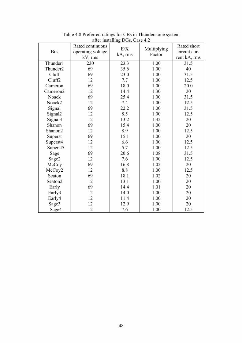
Table 4.8 Preferred ratings for CBs in Thunderstone system after installing DGs, Case 4.2
Bus Rated continuous operating voltage
kV, rms
E/X kA, rms
Multiplying Factor
Rated short circuit cur-
rent kA, rms Thunder1 Thunder2
Cluff Cluff2
Cameron Cameron2
Noack Noack2 Signal Signal2 Signal3 Shanon Shanon2 Superst Superst4 Superst5
Sage Sage2
McCoy McCoy2 Seaton Seaton2
Early Early3 Early4 Sage3 Sage4
230 69 69 12 69 12 69 12 69 12 12 69 12 69 12 12 69 12 69 12 69 12 69 12 12 12 12
23.3 35.6 23.0 7.7 18.0 14.4 25.4 7.4 22.2 8.5 13.2 15.4 8.9 15.1 6.6 5.7 20.6 7.6 16.8 8.8 18.1 13.1 14.4 14.0 11.4 12.9 7.6
1.00 1.00 1.00 1.00 1.00 1.30 1.00 1.00 1.00 1.00 1.32 1.00 1.00 1.00 1.00 1.00 1.08 1.00 1.02 1.00 1.02 1.00 1.01 1.00 1.00 1.00 1.00
31.5 40
31.5 12.5 20.0 20
31.5 12.5 31.5 12.5 20 20
12.5 20
12.5 12.5 31.5 12.5 20
12.5 20 20 20 20 20 20
12.5
48
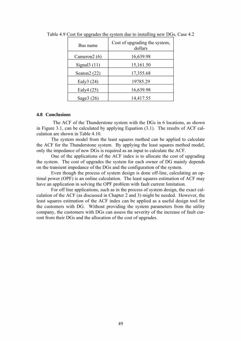
Table 4.9 Cost for upgrades the system due to installing new DGs, Case 4.2
Bus name Cost of upgrading the system, dollars
Cameron2 (6) 16,639.98
Signal3 (11) 15,161.50
Seaton2 (22) 17,355.68
Ealy3 (24) 19785.29
Ealy4 (25) 16,639.98
Sage3 (26) 14,417.55
4.8 Conclusions The ACF of the Thunderstone system with the DGs in 6 locations, as shown
in Figure 3.1, can be calculated by applying Equation (3.1). The results of ACF cal-culation are shown in Table 4.10.
The system model from the least squares method can be applied to calculate the ACF for the Thunderstone system. By applying the least squares method model, only the impedance of new DGs is required as an input to calculate the ACF.
One of the applications of the ACF index is to allocate the cost of upgrading the system. The cost of upgrades the system for each owner of DG mainly depends on the transient impedance of the DGs and the configuration of the system.
Even though the process of system design is done off-line, calculating an op-timal power (OPF) is an online calculation. The least squares estimation of ACF may have an application in solving the OPF problem with fault current limitation.
For off line applications, such as in the process of system design, the exact cal-culation of the ACF (as discussed in Chapter 2 and 3) might be needed. However, the least squares estimation of the ACF index can be applied as a useful design tool for the customers with DG. Without providing the system parameters from the utility company, the customers with DGs can assess the severity of the increase of fault cur-rent from their DGs and the allocation of the cost of upgrades.
49

Ta
ble
4.10
The
ave
rage
cha
nge
of fa
ult c
urre
nt (A
CF)
due
to in
stal
ling
new
DG
into
the
Thun
ders
tone
syst
em, C
ase
4.1
New
DG
at B
us
Out
put o
f DG
, M
VA
Pe
netra
tion
Leve
l (%
) A
CF1
(%)
Incr
emen
t of
AC
F
(%)
Max
imum
C
hang
e of
Fau
lt cu
rren
t1 (%)
At b
us2
6 6+
11
6+11
+22
6+11
+22+
24
6+11
+22+
24+2
5 6+
11+2
2+24
+25+
26
25
25+1
9.1
25+1
9.1+
20.2
25
+19.
1+20
.2+2
0.0
25+1
9.1+
20.2
+20.
0+7.
9 25
+19.
1+20
.2+2
0.0+
7.9+
15.1
9.2
16.4
24
.1
31.7
34
.8
40.6
1.73
3.
43
5.39
7.
66
9.43
10
.87
1.73
1.
70
1.96
2.
27
1.77
1.
44
3.85
5.
01
6.82
9.
98
14.0
2 15
.08
5 5 21
23
23
23
N
otes
1.
U
sing
con
vent
iona
l fau
lt ca
lcul
atio
n 2.
C
onsi
der o
nly
the
bus w
ithou
t ins
talli
ng D
G
50

5. Implication of Fault Current Increase on Optimal Power Flow
5.1 Implications of fault current in an OPF There are several major objectives of calculating an OPF. One objective is to
minimize the generation cost and calculate optimal setting for each generator in serving the load demand. Another objective is providing the information on economic analyses of the power system by determining the marginal cost data. In some application, the minimum fuel cost OPF is sufficient for obtaining power dispatch. The OPF can also in-clude constraints that represent in the operation of the system, such as transmission ca-pacity, voltage security and system stability. In this analysis, the fault current limitation is added as a constraint to the OPF. The ability of including different constraints and objec-tive functions is sometimes needed in power system analysis. References [1, 35, 41] give an introduction to the OPF of electric power systems.
As discussed in Chapters 2 and 3, higher penetration levels due to installing DGs causes the increase of fault current. The increase of fault current may create problems during a fault, such as the potentially inappropriate setting of protection systems, nui-sance trips and inadequate interruption capability of CBs. Fault current can be consid-ered as a constraint in the OPF problem which may limit the operation of power systems. Many techniques can be applied to solve the OPF problem, such as the lambda iteration method, gradient methods, Newton’s method, linear programming method (LPOPF) and the interior point method.
The example in this chapter introduces a totally preliminary study on the operat-ing implications imposed by increased fault current due to the addition of DGs and/or merchant plans to a power system. The Thunderstone system (see Chapter 3 and Appen-dix A) is used to demonstrate a potential economic impact due to the high levels of DG and merchant plant penetration.
5.2 An illustration of operating implications of fault current In this demonstration, four merchant plants are installed in the 69 kV bus of the
Thunderstone system. This example is denominated as Case 5.1. In Case 5.1, operating limitations due to fault current are not included. In Case 5.2, the identical conditions to Case 5.1 are used except that fault current limit will be included. Table 5.1 shows the data of several merchant plants. These merchant plants are fictitious generating sources that are assumed to be available to operators of the Thunderstone system. Figure 5.1 shows the incremental fuel cost curves for the four merchant plants.
51

Table 5.1 Merchant plant data: Cases 5.1 and 5.2 (100 MVA base) Location of
merchant plant Maximum capacity
(MW) Cost function
($/MWh) λ,DGz (p.u.) *
Superstition (14) 50 CF(P1) = 14.020 P+ j0.1388
Early (23) 20 CF(P1) = 220 P+ j0.69
Signal (9) 10 CF(P1) = 3220 P+ j0.69
Cameron (5) 10 CF(P1) = 46100 P+ j0.30
The connection of these merchant plants to the Thunderstone system increases the fault current throughout the system. In some cases, especially when the system has high penetration level, the fault current after connecting these merchant plants may be higher than the interrupting capability of some CBs in the system. This means that the CBs may fail to interrupt fault current and may create a safety hazard.
Figure 5.1 Incremental fuel cost of the merchant plants for Case 5.1 and 5.2
Assume that the interrupting capability of the CBs before connecting these mer-chant plants to the Thunderstone system is chosen as shown in Table 4.7 in Chapter 4. Example 5.1, four merchant plants are installed in the Thunderstone system. As shown in Table 5.2, there are 24 or 16 possible combinations of connecting these merchant plants. That is the operating status off, off, off, off to on, on, on, on represent 16 possible combinations. After analyzing the increase of fault current and resizing the CBs at each bus for all 16 cases by utilizing the technique discussed in Chapters 2 and 4, it is found that there are eight combinations such that some CBs in the system need to be upgraded. If the interrupting capability of the CBs is considered to be a constraint in the OPF prob-lem, only seven combinations listed in Table 5.2 meet this constraint.
The following section compares the cost of generating at these merchant plants with and without the fault current limit as a constraint. For the ease of demonstration, the solution of this problem is done by the Equal Incremental Cost (EIC) technique and the results are shown in the following section.
Incr
emen
tal F
uel C
ost (
$ / M
Wh)
F4(P4) = 100 + 6P4
F3(P3) = 20 + 2P3 F2(P2) = 20 + P2
F1(P1) = 20 + 0.4P1
Pi (MW)0 10 20 30 40 50 60
20406080
100
120140160180200
52

Operational cost without fault current limitation: Case 5.1 Suppose these four merchant plants are requested to deliver a total power at 25
MW. The conditions for an optimum dispatch are, λ=+ 14.020 P
λ=+ 220 P λ=+ 3220 P
and 25321 =++ PPP .
In these equations, Pi is the generation at unit i in MW, and λ is the “system lambda” (i.e., the equal incremental cost of all cycling generation units [1, 35]). Solving the above equations,
λ = 26.25 $/MWh P1 = 15.625 MW P2 = 6.25 MW P3 = 3.125 MW
P4 = 0 MW.
The optimum dispatch schedule for versus the total merchant plant generation is shown in Figure 5.2. The incremental cost is shown in Figure 5.3. The operating cost of generat-ing a total of 25 MW is
( ) 125.578)25(2025.2621
=+ $/h
Note that the operating cost can be represented graphically by the shaded area in Figure 5.3.
Operational cost with fault current limitation: Case 5.2 According to Table 5.2, the fault current limit constraint forces the Units 1, 2 and
3 not to serve at the same time. In order to serve the demand within the constraint, the possible solutions are serving the load by only Unit 1 or by a combination of Units 2 and 3. The constrained case is denominated as Case 5.2
Suppose Unit 1 is set to serve the total demand of 25 MW, the conditions for op-timal dispatch are,
λ=+ 14.020 P and P1 = 25 MW. The incremental cost, λ, is 30.0 $/MWh and the operating cost is 625.0 $/h.
53

0 10 20 30 40 50 60 70 80 90 100 110 120
10
20
30
40
50
Unit 1P i
(MW
)
Unit 2
Unit 3
Unit 4
PT (MW)
Figure 5.2 Economic dispatch for all units (without fI condition): Case 5.1
0 20 40 60 80 100
20
40
60
80
100
120
140
160
Incr
emen
tal c
ost,
λ ($
/ M
Wh)
Operating cost at 25 MW
Pi (MW) Figure 5.3 Incremental cost curve (without fI condition): Case 5.1
54

Suppose Units 2 and 3 are set to serve the total demand. The optimal con-
ditions are, λ=+ 220 P
λ=+ 3220 P and
P2 + P3 = 25 MW . Solving the equations,
λ = 36.67 $/MWh P2 = 16.67 MW P3 = 8.33 MW
and the incremental cost, λ, is 36.67 $/MWh.
Table 5.2 Limitation of the system operation due to the increase of fault current, Case 5.2 Merchant plant locations (Connect / Disconnect Χ)
Superstition (14) Cameron (5) Signal (9) Ealy (23)
fI within
CB limit
Χ Χ Χ Χ Y
Χ Χ Χ Y
Χ Χ Χ Y
Χ Χ Y
Χ Χ Χ Y
Χ Χ Y
Χ Χ Y
Χ N
Χ Χ Χ Y
Χ Χ N
Χ Χ N
Χ N
Χ Χ N
Χ N
Χ N
N
55

The cost of operation when Units 2 and 3 are in service is
( =+ 2520667.3621 ) 708.33 $/h.
The optimum schedule for Case 5.2 when Units 2 and 3 are in service and the incre-mental cost of operation are shown in Figures 5.4 and 5.5.
0 10 20 30 40
5
10
15
20 Unit 2
P i (
MW
)
Unit 3
PT (MW) Figure 5.4 Economic dispatch for all units (with fI condition) when Unit 2 and 3 are in
service, Case 5.2
Figure 5.5 Incremental cost curve (with fI condition), Case 5.2
PT (MW)
Incr
emen
tal c
ost,
λ ($
/ M
Wh)
0 10 20 30 40 50
20
40
60
80
Only Unit 1
Unit 2 and 3
56

5.3 Production cost of the merchant plant under the fault current limitation con-straint The calculation of the constrained economic dispatch problem is shown in the
previous section as Case 5.2. Note that serving the total demand of 25 MW by genera-tions at Super, Cameron and Signal is the economic operating point when the fault cur-rent limit is neglected. However, serving the total demand by these three units does not meet the constraint. The constraint makes the system operator serve the demand only by using Unit 1. Table 5.3 shows the summary of the operating cost of merchant plants in Case 5.2.
Table 5.3 Operating cost of serving the demand: Case 5.2 Merchant plant locations ( Connect / Disconnect X) Operating cost of serving loads ($/h)
Super (14) Cameron (5) Signal (9) Ealy (23) 10 MW 25 MW 50 MW
Χ Χ 233.3 708.3 -
Χ Χ Χ 220.0 625.0 1,500.0
Χ 212.5 578.1 1,312.5
5.4 Conclusions New developments in deregulation have brought new generation sources, such as In-
dependent Power Producers (IPPs) and DGs, to the system. IPPs and increased interconnec-tion to utilize power from interchanges are new factors in fault current calculation. This chapter contains a preliminary illustration of the influence of fault current on the operating conditions of power systems. It demonstrated the potential economic impact arising from the increase of fault current due to the interconnection of new merchant plants. The case study shows that the generation of the merchant plants under the fault current limitation may result in higher cost of operation than the operation without this constraint.
57

6. Conclusions and Recommendations
6.1 Conclusions Fault calculations in power systems are used to determine the interrupting capa-
bility of circuit breakers. The calculation of fault current at the system buses is done by applying the system Zbus matrix. The effects of merchant plants, such as Independent Power Producers, are not taken into consideration in the classical fault current calcula-tion. New developments in deregulation have brought new generation sources to the sys-tem. The appearance of DGs is a cause of increasing fault currents that has not previ-ously been envisioned. This report presents a modification of the conventional fault cur-rent calculation in the case of addition of DGs.
Many consequences arise from increasing of the fault currents, for instance the change of coordination of protective devices, nuisance trips, safety degradation, and the requirement to change recloser and protective relay settings. These consequences result in the cost of equipment upgrades not only at the DG sites but also other system sites.
The equations for calculating the change of fault currents have been provided in Chapter 2 for the balanced three phase case. The Thunderstone system is used to illus-trate the fault current calculation in Matlab. The results of the calculation are presented graphically in Chapter 3 and compared with the solutions from two power system analy-sis software packages: PowerWorld [33] and WinIGS [34].
Due to installing new DGs, six main factors that affect the severity of the increase of three phase fault current at each buses are:
• the number and size of DGs • the operation of the AVR • the impedance of DGs • the location of DGs • the type of DGs • circuit breaker configuration.
Chapter 3 also proposes an index called the average change of fault current or “ACF”. The ACF can be used to indicate the severity of the change of fault current due to installing new DGs. The application of ACF is illustrated in Case 3.3, 4.1 and 4.2. In order to calculate the exact solution of ACF, all system parameters, loads, pre-fault volt-ages and the calculation of fault currents of every bus are required. Chapter 4 proposes the least squares method to approximate the ACF for a given system. By this proposed technique, the pre-fault voltages and the fault current calculation may not be needed in the preliminary design stage. Note that in the preliminary design stage there may be a very large number of calculations, and the ACF concept can speed up the analysis. The only required input of the least squares method is the impedance of a new DG and its lo-cation. The advantages of this technique are:
• faster calculation due to the fact that load flow solution and fault calculations are not required
• contribution of the increase of fault current is indicated at each location of 12 kV bus in the primary distribution system. By this concept, each new DG is treated in an
58

equitable way. The ACF concept is offered as a rapid way to assess fault currents when DGs are deployed in any number, anywhere in the system.
The main disadvantage of the ACF method relates to accuracy. That is, even though the estimator may have been constructed for a large number of sample cases, there is no guarantee that the ACF calculation will be accurate.
The main subjects of this report and “claim of originality” are tabulated in Table 6.1.
Table 6.1 Summary of the topics in this report Topic Innovative concept Classical concept
Fault current calculation
Increasing of fault current due to installing DGs
Calculation of fault current with the present of DGs
CB sizing by E/X method with adjustment of AC and DC increments
Average Change of Fault (ACF) index
Allocation of cost of upgrades
Implication of fault current increase on OPF
6.2 Potential new research areas The following sections are the potential research areas related to power system
fault current due to DGs: The modeling of inverter based DGs
The study of fault current calculations in this report is done by assuming all DGs as synchronous generators. According to the demands for high reliability and power quality for sensitive loads, the demand for renewable generation sources is gradually ris-ing. Renewable generation sources, such as fuel cells, microturbines, solar cells and wind turbines, are mostly based on electronic inverters. These inverter interfaces with the AC network result in changing of the fault response throughout the system. For this reason, the model of inverter based DGs should be included in this study. Included are transient models, single phase / three phase models, and models of the ultimate sources of the electrical energy (e.g. a fuel cell or a photovoltaic source). Dollar cost of upgrading
For specific applications of DG, the cost of upgrading protection and interruption devices should be considered. And this dollar cost should be allocated properly. Mini-mizing the upgrade cost is one possibility. Sharing the cost is another alternative. The application of the ACF concept in this report is a further alternative. The economic is-
59

sues need to be analyzed in detail. The nonlinear relationship between fI and CB cost should be considered. Also, issues of the sequencing of DG installations should be con-sidered. For example, if DGs are installed at A, B, and C and cost is allocated; then DGs are installed at D,E, and F, the final stage installation is different than if the installation sequence were A, E, F. Then B, C, D (for example).
Techniques for fault current reduction Perhaps the solution to managing the rising of fault current lies in applying a
technique to reduce the fault current. For example, fault current reduction is possible by installing a reactor in the system. There may also be solid state solutions to this problem. Each alternative needs to be studied in detail.
Security constrained OPF There may be the circumstances in which a security constrained OPF needs to in-
clude constraints imposed by the IC of circuit breakers or the setting of protective relays. Distributed and alternative generation may impact these constraints. The impact of DG on OPF should be analyzed. Although this subject has been addressed in Chapter 5, it seems prudent that a much more detailed analysis of a constrained OPF should be done.
60

References
[1] G. T. Heydt, “Computer methods for power systems,” Stars in a Circle Publica-tions, Scottsdale, AZ, 1996. [2] J. J. Grainger, W. D. Stevenson, “Power system analysis,” McGraw-Hill, New York, 1994. [3] G. W. Stagg, A. H. El-Abiad, “Computer methods in power systems analysis,” McGraw-Hill, New York, 1994. [4] P. M. Anderson, “Analysis of faulted power systems,” IEEE PRESS Power Sys-tem Engineering Series, New York, 1995. [5] The US Department of Energy (DOE), Office of Distributed Energy Resources, www.eere.energy.gov/der/, 2003 [6] IEEE, “Standard for interconnecting distributed resources with electric power sys-tems,” IEEE Standard 1547-2003, 2003. [7] H. B. Püttgen, P. R. Macgregor, F. C. Lambert, “Distributed generation semantic hype or the dawn of a new era,” IEEE Power & Energy Magazine, vol. 1, pp. 22-29, Jan. / Feb. 2003. [8] R. C. Dugan, T. E. McDermott, “Operating conflicts for distributed generation on distribution systems,” Proceedings of the Rural Electric Power Conference, pp. A3/1-A3/6, 2001. [9] Girgis, S. Brahma, “Effect of Distributed generation on protective device coordina-tion in distribution system,” Large Engineering Systems Conference (LESCOPE), Hali-fax NS, pp. 115-119, July 2001. [10] J. G. Slootweg, W. L. Kling, “Impacts of distributed generation on power system transient stability,” Power Engineering Society Summer Meeting, vol. 2, pp. 862-867, 2002. [11] R. C. Dugan, “Issues for distributed generation in the US,” Power Engineering So-ciety Winter Meeting, vol. 1, pp. 121-126, Jan. 2002. [12] R. C. Dugan, “On the necessity of three-phase feeder models for DG planning analysis,” IEEE Power Engineering Society Summer Meeting, vol. 1, pp. 438-441, July 2002 [13] D. Candusso, L. Valero, A. Walter, “Modelling, control and simulation of a fuel cell based power supply system with energy management,” IEEE Annual Conference of Industrial Electronics Society, vol. 2, pp. 1294-1299, Nov. 2002. [14] C. J. Hatziadoniu, A. A. Lobo, F. Pourboghrat, M. Daneshdoost, “A simplified dy-namic model of grid-connected fuel-cell generators,” IEEE Transactions on Power De-livery, vol. 17, no. 2, pp. 467-473, Apr. 2002. [15] T. Petru, T. Thiringer, “Modeling of wind turbines for power system studies,” IEEE Transactions on Power Systems, vol. 17, no. 4, pp. 1132-1139, Nov. 2002. [16] S. Jemeï, D. Hissei, M. C. Péra, J. M. Kauffmann, “Black-box modeling of proton exchange membrane fuel cell generators,” IEEE Annual Conference 28th of Industrial Electronics Society, vol. 2, pp. 1474-1478, Nov. 2002. [17] Y. Fukuyama, Y. Ueki, “Fault analysis system using neural networks and artificial intelligence,” Proceedings of the Second International Forum on Applications of Neural Networks to Power Systems, pp. 20-25, Yokohama, Japan, Apr., 1993.
61

[18] F. B. Lazim, N. Hamzah, P. M. Arsad, “Application of ANN to power system fault analysis,” Proceedings of Student Conference on Research and Development, pp. 269-273, Shah Alam, Malaysia, July, 2002. [19] Distributed Coalition Power of America (DCPA), www.distributed-generation.com, 2002 [20] The Electric Power Research Institute (EPRI), http://www.epri.com/target.asp”, 2002 [21] H. Zareipour, K. Bhattacharya, C. Canizares, “Distributed generation: current status and challenges,” Proceedings of the IEEE North American Power Symposium (NAPS), pp. 392-399, Moscow, Idaho, 2004. [22] Chambers, S. Hamilton, B. Schnoor, “Distributed generation: a nontechnical guide,” PennWell Corporation, Tulsa, Oklahoma, 2001. [23] T. Ackerman, G. Anderson, L. Soder, “Distributed generation: a definition,” Elec-tric Power System Research, vol. 57, pp. 195–204, 2001. [24] “Impact of increasing contribution of dispersed generation on the power system,” CIGRE study Committee no. 37, Final Report, 2003. [25] J. Larminie, A. Dicks, “Fuel cell system explained,” John Wiley & Sons, West Sussex, England, 2003. [26] G. Hoogers, “Fuel cell technology handbook,” CRC Press, Boca Raton, Florida, 2002. [27] L. Castaner, S. Silvestre, “Modeling photovoltaic systems using PSpice,” John Wiley & Sons, West Sussex, England, 2002. [28] Arizona Public Service (APS), “Arizona PV cost,” www.solarelectricpower.org, 2003 [29] IEEE, “Rating structure for AC high-voltage circuit breakers,” IEEE Standard C37.04, 1999. [30] IEEE, “Application guide for AC high-voltage circuit breakers rated on a sym-metrical current basis,” IEEE/ANSI Standard C37.010, 1999. [31] ANSI, “AC high-voltage circuit breakers rated on a symmetrical current basis – preferred ratings and related required capabilities,” ANSI Standard C37.06, 1997. [32] N. Nimpitiwan, G. T. Heydt, “Fault current issues for market driven power sys-tems with distributed generation,” Proceedings of the North American Power Symposium (NAPS), pp. 400-406, Moscow, Idaho 2004. [33] PowerWorld Corporation, www.powerworld.com, 2004. [34] S. Meliopoulos, “WinIGS: integrated grounding system design program,” Georgia Tech, March, 2004. [35] Wood, B. Wollenberg, “Power generation operation and control,” second edition, Wiley Interscience Publication, New York, 1996. [36] ANSI, “Electric power systems and equipment - voltage ratings (60 Hz),” ANSI Standard C84.1, 1995. [37] S. Haykin, “Neural networks: a comprehensive foundation,” second edition, Pren-tice Hall, New York, 1999. [38] D. Montgomery, E. Peck, G. Vining, “Introduction to linear regression analysis,” third edition, Wiley Series in Probability and Statistics, New York, 2001. [39] M. Huneault, F. D. Galiana, “A survey of the optimal power flow literature,” IEEE Transactions on Power Systems, vol. 6, No. 2, pp. 762-770, May 1991.
62

[40] P. Venkataraman, “Applied optimization with Matlab programming,” Wiley In-terscience, New York, 2001. [41] M. E. El-Hawary, G. S. Christeiensen, “Optimal economic operation of electric power systems,” Academic Press, New York, 1987. [42] D. Gan, R. J. Thomas, R. D. Zimmerman, “Stability-constrained optimal power flow,” IEEE Transactions on Power Systems, vol. 15, no. 2, pp. 535-539, May 2000. [43] A. A. El-Keib, H. Ma, J. L. Hart, “Environmentally constrained economic dispatch using lagrangian relaxation method,” IEEE Transactions on Power Systems, vol. 9, no. 4, pp. 1723-1729, Nov. 1994. [44] R. Ramanathan, “Emission constrained economic dispatch,” IEEE Transac-tions on Power Systems, vol. 9, no. 4, pp. 1994-2000, Nov. 1994. [45] K. P. Wong, J. Yuryevich, “Evolutionary programming based algorithm for environmentally constrained economic dispatch,” IEEE Transactions on Power Systems, vol. 13, no. 2, pp. 301-306, May 1998. [46] K. Deb, “Multi objective optimization using evolutionary algorithms,” Wiley Interscience series in systems and optimization, New York, 2001. [47] T. Yalcinoz, H. Altun, “Environmentally constrained economic dispatch via a genetic algorithm with arithmetic crossover,” IEEE Africon, pp. 923-928, 2002. [48] H. Ma, A. A. El-Keib, R. E. Smith, “A genetic algorithm based approach eco-nomic dispatch of power systems,” International Conference on Power Industry Com-puter Applications, pp. 207-212, May 2001. [49] W. F. Tinney, J. M. Bright, K. D. Demaree, B. A. Hughes, “Some deficiencies in optimal power flow,” IEEE Transactions on Power Systems, vol. 3, no. 2, pp. 676-683, May 1988. [50] K. C. Almeida, F. D. Galiana, “Critical cases in the optimal power flow,” IEEE Transactions on Power Systems, Vol. 11, no. 3, pp. 1509-1518, Aug. 1994. [51] B. H. Chowdury, S. Rahman, “A review of recent advances in economic dis-patch,” IEEE Transactions on Power Systems, vol. 5, no. 4, pp. 1248-1259, Nov. 1990. [52] M. Huneault, F. D. Galiana, “A survey of the optimal power flow literature,” IEEE Transactions on Power Systems, vol. 6, no. 2, pp. 762-770, May 1991. [53] Y. Jiang, S. Dongyuan, D. Xianzhong, T. Yuejin, C. Shijie, “Comparison of superconducting fault current limiter in power system,” Proceedings of Summer Meeting, Power Engineering Society, vol. 1, pp. 43-47, Jul. 2001. [54] E. M. Lueng, “Superconducting fault current limiters,” IEEE Power Engineer-ing Review, vol. 10, no. 8, pp. 15-18, Aug. 2000. [55] A. J. Power, “An overview of transmission fault current limiters,” IEE Collo-quium, pp. 1/1-1/5, Jun. 1995. [56] X. Wu, J. Mutale, N. Jenkins, G. Strbac, “An investigation of network split-ting for fault level reduction,” Technical report, Tyndal center of climate change re-search, Manchester Center for Electric Energy, Sep. 2003, http://www.tyndall.ac.uk/publications/working_papers/wp25.pdf. [57] M. Sjöström, R. Cherkaoui and B. Dutoit, “Enhancement of power system transient stability using superconducting fault current limiters,” IEEE Transactions on Applied Superconductivity, vol. 9, no. 2, pp. 1328-1330, Jun. 1999.
63

[58] S. Lee, C. Lee, T. Ko, O. Kyun, “Stability analysis of a power system with superconducting fault current limiter installed,” IEEE Transactions on Applied Super-conductivity, vol. 11, no. 1, pp. 2098-2101, Mar. 2001. [59] K. Hongesomebut, Y. Mitani, K. Tsuji, “Optimal location assignment and de-sign of superconducting fault current limiters applied to loop power systems,” IEEE Transactions on Applied Superconductivity, vol. 13, no. 2, pp. 1828-1831, Jun. 2003. [60] L. Ye, L. Lin, K. Juengst, “Application studies of superconducting fault cur-rent limiters in electric power system,” IEEE Transactions on Applied Superconductivity, vol. 12, no. 1, pp. 900-903, Mar. 2002. [61] E. Calixte, Y. Yokomizu, H. Shimizu, T. Matsumura, H. Fujita, “Reduction of rating required for circuit breakers by employing series connected fault current limiters,” IEE Proceedings on Generation, Transmission and Distribution, vol. 151, no. 1, pp. 36-42, Jan. 2004. [62] G. G. Karady, “Principles of fault current limitation by a resonant LC circuit,” IEE Proceedings on Generation, Transmission and Distribution, vol. 139, no. 1, pp. 1-6, Jan. 1992. [63] H. W. Dommel, W. F. Tinney, “Optimal Power Flow Solutions,” IEEE Trans-actions on Power Apparatus and Systems, vol. PAS-87, pp. 1866-1867, Oct. 1968.
64

Appendix A
SYSTEM PARAMETERS OF THE THUNDERSTONE SYSTEM
This appendix shows the detail of system parameters of the Thunderstone system, such as line parameters, transformer impedance, loads and impedance of DGs. All pa-rameters are used in the experiments in Chapter 3 and Chapter 4.
Table A.1 Transmission line parameter for Thunderstone system
69 kV Line Per unit impedance @100°C (100 MVA Base)
FROM TO R1 X1 G1 B1 G2 B2
1 Cluff Thundrst 0.00232 0.01552 0 0.0004
2 Cluff Cameron 0.00253 0.01636 0 0.00044 0 0.00046
3 Superst3 Cameron 0.01245 0.07996 0 0.00223 0 0.00223
4 Noak Thundrst 0.00235 0.01295 0 0.00035 0 0.00034
5 Noak SignalBu 0.00439 0.024 0 0.00064 0 0.00065
6 Shannon SignalBu 0.00756 0.03097 0 0.00038 0 0.00038
7 Shannon Superst4 0.00861 0.03572 0 0.00045 0 0.00045
8 SignalBu Thundrst 0.01562 0.05749 0 0.00076
9 Seaton SignalBu 0.00868 0.03194 0 0.00042
10 Sage Thundrst 0.00436 0.02435 0 0.00064 0 0.00063
11 McCoy Sage 0.00691 0.02809 0 0.00035
12 McCoy Seaton 0.00649 0.02638 0 0.00033
13 Ealy Seaton 0.00869 0.03517 0 0.00043 0 0.00043
14 Ealy Superst1 0.01113 0.04134 0 0.00054
65

Table A.2 Load bus data Bus MW MVAR
Cluff 22 0.5
Cameron 27.1 0.5
Noack 21.6 0.8
SignalBU 43.8 2.1
Bay 3 22.3 0.3
Bay 4 21.5 1.8
Shanon 23.3 2.3
Superstition 39.6 3
Bay 2 16 3.2
Bay 3 23.6 0.2
Sage 56.4 6.5
Seaton 23.2 2.6
Ealy 30 2.4
Bay 2 21.4 0.4
Bay 4 8.6 2
McCoy 0 0
Table A.3 Substation transformer (230/69 kV) at Thunderstone substation PU on a 100 MVA base
R X Bmag
0.002 0.06 0
0.001 0.06 0
0.001 0.07 0
0.001 0.06 0
66

Table A.4 Distribution transformers p.u. at Rated MVA
FROM Bus kV To Bus
kV Rated MVA R X
Bmag
Cluff 69 Cluff LD1 12 12 0.024 0.0742 0
Cameron 69 Cameron LD1 12 15 0.02 0.078 0
Ealy LD1 69 Ealy LD2 12 15 0.0198 0.0779 0
Ealy LD2 69 Ealy LD4 12 10 0.0388 0.074 0
Mccoy 69 Mccoy LD2 12 15 0.0197 0.0758 0
Noack 69 Noack LD2 12 12 0.0232 0.076 0
Sage 69 Sage LD2 12 12.5 0.0422 0.0725 0
Sage 69 Sage LD3 12 12.5 0.0228 0.0744 0
Sage 69 Sage LD4 12 12.5 0.0228 0.0741 0
Seaton 69 Seaton LD1 12 12 0.0238 0.0733 0
Shanon 69 Shannon LD2 12 15 0.0198 0.0763 0
SignalBU 69 Signal LD3 12 12 0.037 0.069 0
SignalBU 69 Signal LD4 12 12 0.0243 0.073 0
Superstition 69 Superstition LD2 12 12 0.0233 0.083 0
Superstition 69 Superstition LD3 12 12 0.0239 0.1028 0
67

Appendix B
LIST OF CONDITIONS FOR ALL THE EXPERIMENTS
This appendix shows the summary of the experiment in this report. All experi-ments in Chapter 3 and Chapter 4 are simulated based on the Thunderstone system.
Table B.1 Summary of the case studies
Case Locations of DG Varied parameters Target of experiments
3.1
Cameron2
Signal3
Sage3
Seaton2
Number and locations of DGs in the system
Severity of the change of fault current
3.2
Seaton
Cameron2
Signal3
Sage3
AVR turn on/off Severity of the change of fault current
3.3
Cameron2
Signal3
Sage3
Seaton2
Impedance of DGs Severity of the change of fault current
4.1
Cameron2
Signal3
Seaton2
Ealy3
Ealy4
Sage3.
Impedance of DGs, loca-tion of new DGs
Illustrates application of the least squares
estimator to calculate the ACF
68

Table B.1 Summary of the case studies (cont.)
Case Locations of DG Varied parameters Target of experiments
4.2
Cameron2
Signal3
Seaton2
Ealy3
Ealy4
Sage3.
Impedance of DGs, loca-tion of new DGs
Shows the bus loca-tions which need to be
upgraded
5.1
Superstition (14)
Early (23)
Signal (9)
Cameron (5)
Without considering the operating limitations
Operating implication imposed by the in-crease fault current
5.2
Superstition (14)
Early (23)
Signal (9)
Cameron (5)
Consider the operating limitations
Operating implication imposed by the in-crease fault current
69