connections between physical, optical and biogeochemical...

Progress in Oceanography 122 (2014) 30–53

Contents lists available at ScienceDirect

Progress in Oceanography

journal homepage: www.elsevier .com/locate /pocean

Connections between physical, optical and biogeochemical processesin the Pacific Ocean

0079-6611/$ - see front matter � 2013 Elsevier Ltd. All rights reserved.http://dx.doi.org/10.1016/j.pocean.2013.11.008

⇑ Corresponding author. Address: School of Marine Sciences, University of Maine5706 Aubert Hall, Orono, ME 04469, USA. Tel.: +1 207 5814349.

E-mail address: [email protected] (P. Xiu).

Peng Xiu ⇑, Fei ChaiSchool of Marine Sciences, University of Maine, Orono, ME 04469, USA

a r t i c l e i n f o

Article history:Received 1 January 2013Received in revised form 19 November 2013Accepted 25 November 2013Available online 6 December 2013

a b s t r a c t

A new biogeochemical model has been developed and coupled to a three-dimensional physical model inthe Pacific Ocean. With the explicitly represented dissolved organic pools, this new model is able to linkkey biogeochemical processes with optical processes. Model validation against satellite and in situ dataindicates the model is robust in reproducing general biogeochemical and optical features. Colored dis-solved organic matter (CDOM) has been suggested to play an important role in regulating underwaterlight field. With the coupled model, physical and biological regulations of CDOM in the euphotic zoneare analyzed. Model results indicate seasonal variability of CDOM is mostly determined by biological pro-cesses, while the importance of physical regulation manifests in the annual mean terms. Without CDOMattenuating light, modeled depth-integrated primary production is about 10% higher than the control runwhen averaged over the entire basin, while this discrepancy is highly variable in space with magnitudesreaching higher than 100% in some locations. With CDOM dynamics integrated in physical-biologicalinteractions, a new mechanism by which physical processes affect biological processes is suggested,namely, physical transport of CDOM changes water optical properties, which can further modify under-water light field and subsequently affect the distribution of phytoplankton chlorophyll. This mechanismtends to occur in the entire Pacific basin but with strong spatial variability, implying the importance ofincluding optical processes in the coupled physical-biogeochemical model.

� 2013 Elsevier Ltd. All rights reserved.

1. Introduction

Light distribution below the ocean surface has been treated as acontrol mechanism for autotrophic growth. Optical and biogeo-chemical processes are essentially connected via the interactionof light with particulate and/or dissolved matters in the ocean. Un-der a given oceanic environment with ample nutrients, photosyn-thetic organism biomass generally increases with increasing light.As the biomass grows and accumulates, light absorption and scat-tering become stronger, leading to less light penetration in thewater, which in turn provides a negative feedback for the biologicalactivities (Yentsch and Phinney, 1989; Bissett et al., 2001; Roth-stein et al., 2006). The impacts of physical processes on biogeo-chemical processes have been primarily recognized as horizontaland/or vertical transports of nutrients and plankton biomass.Changes in optical properties through physical processes, which al-ter underwater light field and further change biological activities,however, are another linkage between physical and biogeochemi-cal processes. Thus, it is important to relate these processes whenassessing marine ecosystem.

Many marine ecosystem models, varying from simple nutrient,phytoplankton, zooplankton, and detritus (NPZD) models to com-plex models with 20 or more components (e.g., Chai et al., 2002;Moore et al., 2002; Anderson and Pondaven, 2003; Aumont et al.,2003; Fennel et al., 2003; Goebel et al., 2010) often use an approx-imation of integrated photosynthetically active radiation (PAR,400–700 nm) that only attenuates with phytoplankton biomass(or chlorophyll) and seawater to control the assimilation of inor-ganic nutrients. Such a simplification in relationship between lightattenuation and phytoplankton biomass is easy to implement fornumerical calculation and biological consideration. However, con-siderable nonlinearity exists when considering phytoplanktonsizes and their photo-adaptive states (Smith and Baker, 1978; Bri-caud et al., 1983). In addition to phytoplankton, detritus and col-ored dissolved organic matter (CDOM) absorption and particulatebackscattering, referred to as inherent optical properties that areoften not represented in ecosystem models can affect underwaterlight field as well (e.g., Babin et al., 2003a;Boss et al., 2004).

Adding optics to an ecosystem model has been suggested to bemore accurate in generating subsurface light field (Fujii et al.,2007). Directly comparing modeled optical properties with oceancolor and in situ data also gives additional constraints on modelparameters to reduce uncertainties in model simulations, as manysatellite-derived products, such as chlorophyll concentration,

http://crossmark.crossref.org/dialog/?doi=10.1016/j.pocean.2013.11.008&domain=pdf

http://dx.doi.org/10.1016/j.pocean.2013.11.008

mailto:[email protected]

http://dx.doi.org/10.1016/j.pocean.2013.11.008

http://www.sciencedirect.com/science/journal/00796611

http://www.elsevier.com/locate/pocean

P. Xiu, F. Chai / Progress in Oceanography 122 (2014) 30–53 31

carbon biomass, and primary production, are estimated based onempirical or semi-analytical algorithms linking with ocean optics(IOCCG, 2006). However, only few ecosystem models have consid-ered the optical processes associated with underwater light field(e.g., Bissett et al., 1999a; Fujii et al., 2007). The one-dimensional(1-D) ecosystem model developed by Fujii et al. (2007) is able tosimulate underwater light field and the feedbacks to biologicalprocesses. The CDOM that is not included in their model, however,may have an important role in regulating phytoplankton dynamicsand nutrient cycling in the euphotic zone. The production anddestruction mechanisms for CDOM include phytoplankton exuda-tion, zooplankton messy feeding, detritus breakdown, bacterialproduction and consumption, and photolysis by ultraviolet (UV,280–400 nm) light, which are fundamentally different and decou-pled from those for phytoplankton, especially in coastal regionswhere terrestrial CDOM is introduced. To incorporate CDOM inan ecosystem model, one must consider the cycling of dissolvedmatter pool and the microbial loop in the ocean in addition tothe classic NPZD processes.

The objective of this study is to develop an ecosystem modelthat explicitly describes wavelength-resolved optical properties(visible light, 400–700 nm), associated with multi-nutrient phyto-plankton, zooplankton, and detritus. We also include the photo-acclimation process for phytoplankton in the model to better re-solve the dynamic link between phytoplankton chlorophyll andcarbon biomass. Carbonate system, including dynamics of totalalkalinity, ocean calcification and the air-sea gas exchange of car-bon dioxide, is explicitly represented as well. We couple this modelto the Pacific Ocean (45�S to 65�N, 100�E to 70�W) with a three-dimensional (3-D) general circulation model. The model perfor-mance is examined by comparing model outputs with available sa-tellite and in situ data. Numerical experiments are conducted tounderstand the dynamic connections between physical, opticaland biogeochemical processes in the Pacific Ocean.

2. Model and data

2.1. Biogeochemical processes

The ecosystem model is primarily based on the Carbon, Silicon,Nitrogen Ecosystem (CoSINE) model (Chai et al., 2002). We followprevious approaches to simulate phytoplanktonic photo-acclima-tion and the dynamic chlorophyll-to-carbon ratio under differentgrowth conditions (Geider et al., 1998; Moore et al., 2002; Fujiiet al., 2007). The ecosystem consists of 31 state variables describ-ing three phytoplankton functional groups in three different bio-mass forms, picoplankton nitrogen, carbon and chlorophyll (P1,C1, Chl1), diatoms nitrogen, carbon and chlorophyll (P2, C2,Chl2), and coccolithophorids nitrogen, carbon and chlorophyll(P3, C3, Chl3); two size classes of zooplankton, microzooplanktonnitrogen (Z1), mesozooplankton nitrogen (Z2), and their carbonterms (ZC1, ZC2); detritus in terms of particulate organic nitrogen(PON), particulate organic carbon (POC), particulate inorganic car-bon (PIC) and biogenic silica (bSiO2); silicate (Si(OH)4); phosphate(PO4); dissolved oxygen (DO); total alkalinity (TALK); total CO2

(TCO2); two forms of dissolved inorganic nitrogen, nitrate (NO3)and ammonium (NH4); bacteria nitrogen (BAC); as well as dis-solved organic matter, labile dissolved organic nitrogen (LDON), la-bile dissolved organic carbon (LDOC), colored labile dissolvedorganic carbon (CLDOC), semi-labile dissolved organic nitrogen(SDON), semi-labile dissolved organic carbon (SDOC), and coloredsemi-labile dissolved organic carbon (CSDOC) (Fig. 1). The govern-ing equations and formulations of biogeochemical processes aredenoted in Appendix A, and a list of parameters used in the modelis provided in Table 1.

Nutrient uptake and photosynthetic rate are modeled as func-tions of environmental factors and cellular composition (C:Chland C:N). The model includes down-regulation of pigment contentat high irradiance or when growth rate is limited by nutrients andtemperature, and feedback between nitrogen and carbon metabo-lism (Geider et al., 1998). Phytoplankton ratios (C:Chl and C:N)vary dynamically between maximum and minimum cell quotasaccording to the changes in light and nutrient levels (Xiu and Chai,2012). The maximum and minimum cell quotas for different phy-toplankton functional groups are chosen based on Moore et al.(2002) and Fujii et al. (2007).

All phytoplankton take up NO3, NH4, PO4 and TCO2 for photo-synthesis. Diatoms also take up Si(OH)4 for the silicification pro-cess, and coccolithophorids utilize TALK and TCO2 for thecalcification process (Fujii and Chai, 2007). The microzooplanktongraze on picoplankton and bacteria. The mesozooplankton feedon diatoms, coccolithophorids, microzooplankton, and detritus.The remineralization of organic nitrogen, silicon and carbon, bothinside and below the euphotic zone, is a critical process for nutri-ent recycling efficiency. It depends on a number of factors, includ-ing water temperature, nutrient condition, particle sizes andzooplankton grazing (Ragueneau et al., 2000; Ward, 2000). Theremineralization of organic nitrogen is primarily biological with arapid production of NH4 and TCO2 through zooplankton grazingin the euphotic zone and bacteria decomposition of organic matterbelow the euphotic zone. Below the euphotic zone, sinking partic-ulate organic matter (POM) is converted to inorganic nutrients anddissolved organic matter (DOM) by a regeneration process.Through the dissolution process, a majority of the POM is con-verted to inorganic nutrients (90%), and the rest goes into theDOM pool.

The DOM pool consists of dissolved organic carbon and nitro-gen. There are a number of processes that can produce and utilizeor remineralize DOM, and most of these processes are poorlyunderstood (Christian and Anderson, 2002). To the first-orderapproximation, DOM processes are modeled as consumption bybacteria and productions by phytoplankton exudation, zooplank-ton messy feeding, and detrital breakdown, as adopted in manystudies (e.g., Anderson and Williams, 1998; Walsh et al., 1999; Tianet al., 2000; Christian and Anderson, 2002; Anderson and Pondav-en, 2003). Phytoplankton exudation representing an active releaseby phytoplankton is modeled as a fraction of primary production.This fraction is highly variable in different studies, with magni-tudes ranging from 2% to 56.4% (Christian and Anderson, 2002).Grazer-related DOM production is modeled as zooplankton messyfeeding, which is a fixed fraction of grazed materials. Among previ-ous studies, this fraction also varies significantly with a range of2.5–50% (Christian and Anderson, 2002). From lab experiments,Strom et al. (1997) estimated that about 16–37% of algal carbonwas released during an ingestion event. Particle dissolution intothe DOM pool with the first-order rate process is used in our mod-el. This approach is a simplified simulation of the underlying mech-anism and has been widely used (e.g., Anderson and Williams,1998; Levy et al., 1998; Vallino, 2000; Yamanaka et al., 2004),although other environmental factors such as temperature, turbu-lence, and bacteria can modify this process.

The primary mechanism for DOM loss is uptake by heterotro-phic bacteria. According to different turnover rates, the DOM is fur-ther divided into labile and semi-labile pools. Labile pool can beconsumed directly by bacteria, while semi-labile pool includesmolecules that require ectoenzyme hydrolysis to be converted tolabile matter. Bacteria utilization of the DOM is modeled by ahyperbolic function that is similar to Michaelis–Menton kinetics(Anderson and Williams, 1998; Anderson and Pondaven, 2003).Bacteria production and remineralization are modeled followingAnderson and Williams (1998) and Walsh et al. (1999). Colored

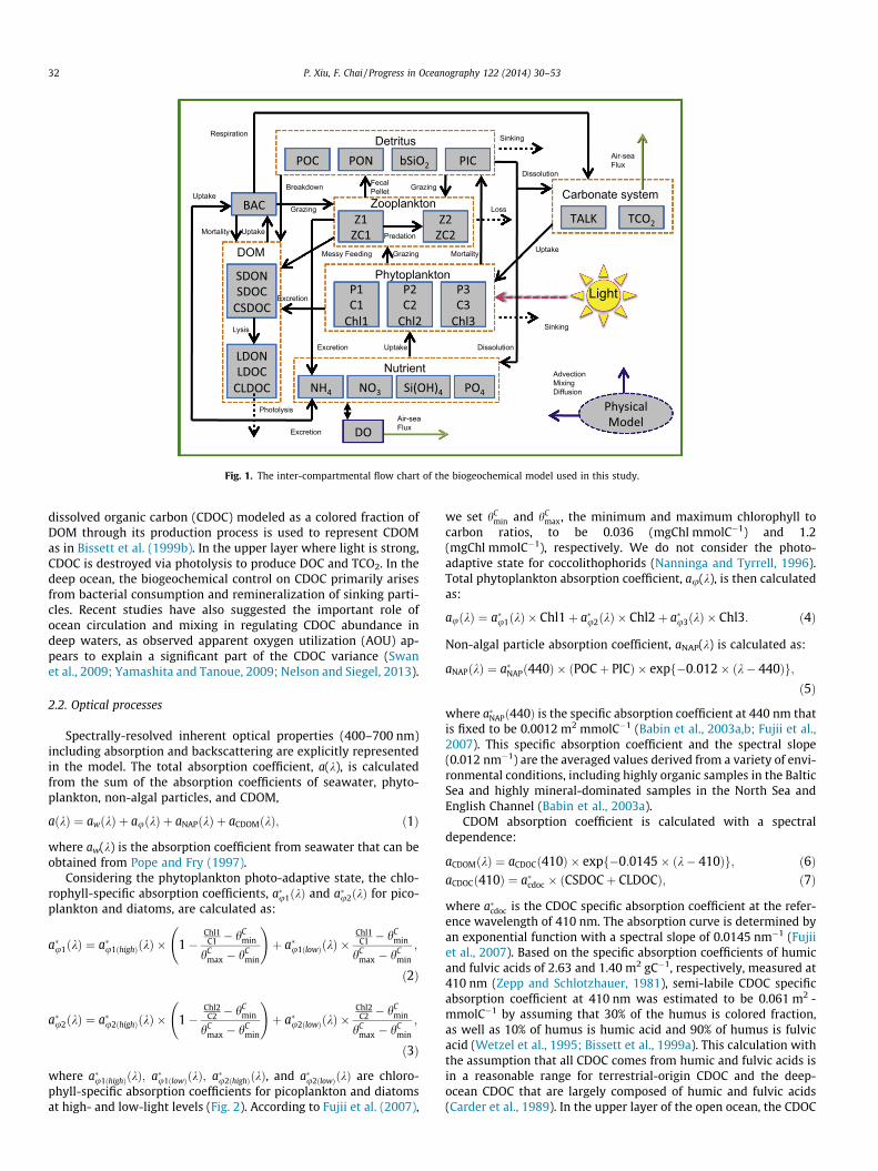
Fig. 1. The inter-compartmental flow chart of the biogeochemical model used in this study.

32 P. Xiu, F. Chai / Progress in Oceanography 122 (2014) 30–53

dissolved organic carbon (CDOC) modeled as a colored fraction ofDOM through its production process is used to represent CDOMas in Bissett et al. (1999b). In the upper layer where light is strong,CDOC is destroyed via photolysis to produce DOC and TCO2. In thedeep ocean, the biogeochemical control on CDOC primarily arisesfrom bacterial consumption and remineralization of sinking parti-cles. Recent studies have also suggested the important role ofocean circulation and mixing in regulating CDOC abundance indeep waters, as observed apparent oxygen utilization (AOU) ap-pears to explain a significant part of the CDOC variance (Swanet al., 2009; Yamashita and Tanoue, 2009; Nelson and Siegel, 2013).

2.2. Optical processes

Spectrally-resolved inherent optical properties (400–700 nm)including absorption and backscattering are explicitly representedin the model. The total absorption coefficient, a(k), is calculatedfrom the sum of the absorption coefficients of seawater, phyto-plankton, non-algal particles, and CDOM,

aðkÞ ¼ awðkÞ þ auðkÞ þ aNAPðkÞ þ aCDOMðkÞ; ð1Þ

where aw(k) is the absorption coefficient from seawater that can beobtained from Pope and Fry (1997).

Considering the phytoplankton photo-adaptive state, the chlo-rophyll-specific absorption coefficients, a�u1ðkÞ and a�u2ðkÞ for pico-plankton and diatoms, are calculated as:

a�u1ðkÞ ¼ a�u1ðhighÞðkÞ � 1�Chl1C1 � hC

min

hCmax � hC

min

!þ a�u1ðlowÞðkÞ �

Chl1C1 � hC

min

hCmax � hC

min

;

ð2Þ

a�u2ðkÞ ¼ a�u2ðhighÞðkÞ � 1�Chl2C2 � hC

min

hCmax � hC

min

!þ a�u2ðlowÞðkÞ �

Chl2C2 � hC

min

hCmax � hC

min

;

ð3Þ

where a�u1ðhighÞðkÞ; a�u1ðlowÞðkÞ; a�u2ðhighÞðkÞ, and a�u2ðlowÞðkÞ are chloro-phyll-specific absorption coefficients for picoplankton and diatomsat high- and low-light levels (Fig. 2). According to Fujii et al. (2007),

we set hCmin and hC

max, the minimum and maximum chlorophyll tocarbon ratios, to be 0.036 (mgChl mmolC�1) and 1.2(mgChl mmolC�1), respectively. We do not consider the photo-adaptive state for coccolithophorids (Nanninga and Tyrrell, 1996).Total phytoplankton absorption coefficient, au(k), is then calculatedas:

auðkÞ ¼ a�u1ðkÞ � Chl1þ a�u2ðkÞ � Chl2þ a�u3ðkÞ � Chl3: ð4Þ

Non-algal particle absorption coefficient, aNAP(k) is calculated as:

aNAPðkÞ ¼ a�NAPð440Þ � ðPOCþ PICÞ � expf�0:012� ðk� 440Þg;ð5Þ

where a�NAPð440Þ is the specific absorption coefficient at 440 nm thatis fixed to be 0.0012 m2 mmolC�1 (Babin et al., 2003a,b; Fujii et al.,2007). This specific absorption coefficient and the spectral slope(0.012 nm�1) are the averaged values derived from a variety of envi-ronmental conditions, including highly organic samples in the BalticSea and highly mineral-dominated samples in the North Sea andEnglish Channel (Babin et al., 2003a).

CDOM absorption coefficient is calculated with a spectraldependence:

aCDOMðkÞ ¼ aCDOCð410Þ � expf�0:0145� ðk� 410Þg; ð6ÞaCDOCð410Þ ¼ a�cdoc � ðCSDOCþ CLDOCÞ; ð7Þ

where a�cdoc is the CDOC specific absorption coefficient at the refer-ence wavelength of 410 nm. The absorption curve is determined byan exponential function with a spectral slope of 0.0145 nm�1 (Fujiiet al., 2007). Based on the specific absorption coefficients of humicand fulvic acids of 2.63 and 1.40 m2 gC�1, respectively, measured at410 nm (Zepp and Schlotzhauer, 1981), semi-labile CDOC specificabsorption coefficient at 410 nm was estimated to be 0.061 m2 -mmolC�1 by assuming that 30% of the humus is colored fraction,as well as 10% of humus is humic acid and 90% of humus is fulvicacid (Wetzel et al., 1995; Bissett et al., 1999a). This calculation withthe assumption that all CDOC comes from humic and fulvic acids isin a reasonable range for terrestrial-origin CDOC and the deep-ocean CDOC that are largely composed of humic and fulvic acids(Carder et al., 1989). In the upper layer of the open ocean, the CDOC

Table 1Model parameters and their values.

Parameters Symbol Chai et al.(2002)

Fujii andChai (2007)

Fujii et al.(2007)

This study Reference

For plankton and zooplanktonNH4 inhibition for P1 w1 5.59 5.59 5.59 5.59 (1), (2), (10)NH4 inhibition for P2 w2 5.59 5.59 5.59 1.5 (1), (6)NH4 inhibition for P3 w3 N/A 5.59 N/A 5.59 (1), (2), (10)Half-saturation for NO3 uptake by P1 KP1_NO3 0.5 1.0 1.0 1.0 (2), (10)Half-saturation for NH4 uptake by P1 KP1_NH4 0.05 0.1 0.05 0.1 (2)Half-saturation for NO3 uptake by P2 KP2_NO3 N/A N/A N/A 3.0 (6)Half-saturation for SiO4 uptake by P2 KP2_SiO4 3.0 3.0 3.0 4.5 (1), (6)Half-saturation for NO3 uptake by P3 KP3_NO3 N/A 1.0 N/A 1.0 (2), (10)Half-saturation for NH4 uptake by P3 KP3_NH4 N/A 1.0 N/A 1.0 (2)P1 mortality c3 N/A N/A N/A 0.02 (1), (6)P2 mortality c4 0.05 0.05 0.05 0.05 (1), (2), (10)P3 mortality c10 N/A 0.05 N/A 0.05 (2)P1, P2, P3 exudation e1, e2, e3 N/A N/A N/A 0.2,0.2,0.2 (4), (5), (6)P1, P2, P3 excretion e4, e5, e6 N/A N/A N/A 0.3,0.3,0.3 (4), (5), (6)P2 sinking speed W1 1.0 1.0 1.0 1.0 (1), (2), (10)P3 sinking speed W3 N/A 1.0 N/A 1.0 (2)Z1 assimilation efficiency for N and C c1 1.0 1.0 1.0 0.9 (1), (6)Z2 assimilation efficiency for N c2 0.75 0.75 0.75 0.7 (1), (6)Z2 assimilation efficiency for C c22 N/A N/A N/A 0.65 (5), (6)Z1 messy feeding fraction U1 N/A N/A N/A 0.1 (4), (5), (6)Z2 messy feeding fraction U2 N/A N/A N/A 0.2 (4), (5), (6)Z1 excretion reg1 0.2 0.2 0.2 0.2 (1)Z2 excretion reg2 0.1 0.1 0.1 0.1 (1)Z2 loss rate k 0.05 0.05 0.05 0.05 (1)Z1 maximum specific grazing rate G1max 1.35 1.25 1.35 1.55 (1), (6)Z2 maximum specific grazing rate G2max 0.53 0.48 0.64 0.56 (1), (6)Half-saturation for Z1 ingestion K1gr 0.5 0.5 0.5 0.5 (1)Half-saturation for Z2 ingestion K2gr 0.25 0.25 0.25 0.25 (1)Z1 grazing preference for P1 q5 1.0 1.0 1.0 0.9 (1), (6)Z1 grazing preference for BAC q6 N/A N/A N/A 0.1 (6)Z2 grazing preference for P2 q1 0.7 0.35 0.7 0.6 (1), (6)Z2 grazing preference for Z1 q2 0.2 0.2 0.2 0.2 (1)Z2 grazing preference for PON q3 0.1 0.1 0.1 0.1 (1)Z2 grazing preference for P3 q4 N/A 0.35 N/A 0.1 (6)Chlorophyll-specific initial slope of P vs. I curve for phytoplankton a N/A N/A 0.25 0.25 (10)Maximum P1 carbon-specific nitrogen-uptake rate PC1

refN/A N/A 2.0 1.5 (10), (6)

Maximum P2 carbon-specific nitrogen-uptake rate PC2ref

N/A N/A 3.0 2.5 (10), (6)

Maximum P3 carbon-specific nitrogen-uptake rate PC3ref

N/A N/A N/A 1.0 (2), (6)

Minimum phytoplankton N:C ratio Qmin N/A N/A 0.034 0.06 (10), (6)Maximum phytoplankton N:C ratio Qmax N/A N/A 0.17 0.17 (10)Maximum value of hN

hNmax

N/A N/A 4.2 1.5 (10), (6)

Other parametersbSiO2 sinking speed W4 20.0 20.0 20.0 20.0 (1)PIC sinking speed W5 N/A 20.0 N/A 15.0 (2), (6)PON sinking speed W6 10.0 10.0 10.0 10.0 (1), (9)POC sinking speed W7 N/A N/A N/A 15.0 (6)Labile fraction of produced DOM b1 N/A N/A N/A 0.8 (5), (6)Labile fraction of phyto-excreted DOC b2 N/A N/A N/A 0.6 (5), (6)Fraction uptake of LDOC by BAC b3 N/A N/A N/A 0.96 (6)Nitrification rate c7 N/A 0.025 0.0 0.05 (2), (6)Cost of biosynthesis nNO3 N/A N/A 2.33 2.33 (10)Color fraction of LDOC colorFR1 N/A N/A N/A 0.1 (11), (6)Color fraction of SDOC colorFR2 N/A N/A N/A 0.2 (11), (6)PON dissolution rate DPON N/A 0.01 0.0 0.01 (2), (8)PIC dissolution rate DPIC N/A 0.005 N/A 0.01 (2), (6)DOM fraction P1, P2, P3 mortality d1, d2, d3 N/A N/A N/A 0.5, 0.5, 0.5 (5), (6)BAC C:N ratio RB N/A N/A N/A 5.1 (5)BAC mortality c12 N/A N/A N/A 0.05 (3), (4), (6)Phosphorus to nitrogen ratio RPN N/A N/A N/A 0.0625 (6)PIC to organic carbon ratio in P3 RCaC N/A 1.0 N/A 1.0 (2)Maximum labile DOC or NH4 uptake lBmax N/A N/A N/A 0.8 (7), (6)Maximum SDOC hydrolysis c13 N/A N/A N/A 0.7 (5), (6)Half-saturation for NH4 uptake KB N/A N/A N/A 0.5 (5)Half-saturation for LDOC uptake KL N/A N/A N/A 25.0 (5)Half-saturation for SDOC uptake KSDOC N/A N/A N/A 417.0 (5)Half-saturation for SDON uptake KSDON N/A N/A N/A 35.3 (6)Respired fraction of BAC growth r_b N/A N/A N/A 0.5 (7)Oxygen to nitrate ratio RO2No3 N/A N/A N/A 8.625 (6)Oxygen to ammonium ratio RO2NH4 N/A N/A N/A 6.625 (6)Specific rate of conversion RtUVLDOC N/A N/A N/A 2.0 (11), (6)Specific rate of conversion RtUVSDOC N/A N/A N/A 2.0 (11), (6)

(continued on next page)


Table 1 (continued)

Parameters Symbol Chai et al.(2002)

Fujii andChai (2007)

Fujii et al.(2007)

This study Reference

Specific rate of conversion RtUVLDIC N/A N/A N/A 4.0 (11), (6)Specific rate of conversion RtUVSDIC N/A N/A N/A 4.0 (11), (6)

(1) Chai et al. (2002), Fujii and Chai (2007); (3) Tian et al. (2000); (4) Anderson and Williams (1998); (5) Anderson and Pondaven (2003); (6) this study; (7) Walsh et al. (1999);(8) Levy et al. (1998); (9) Kishi et al. (2007); (10) Fujii et al. (2007); (11) Bissett et al. (1999a).

0

0.2

0.4

0.6

0.8

1

1.2

1.4

400 450 500 550 600 650 7000

0.01

0.02

0.03

0.04

0.05

0.06

0.07

0.08

0.09

0.1

Wavelength (nm)

a φ* (m2 m

g C

hl−1

)

Nor

mal

ized

aC

DO

M

aφ1*

(low)

aφ1*

(high)

aφ2*

(low)

aφ2*

(high)

aφ3*

Fig. 2. Spectrally-resolved chlorophyll-specific absorption coefficients by picoplankton, diatoms, and coccolithophorids, and the CDOM absorption normalized at 410 nm.Both picoplankton and diatoms are modeled with photoadaption.


pool may also include amino acids and peptides, nucleic acids andbases, and other low-molecular-weight compounds. The specificabsorption coefficients of these components are difficult to estimateas they are usually labile and susceptible to photolysis that mayhave gone through different light histories during different mea-surements. We thus use the same specific absorption coefficientsfor both labile and semi-labile CDOCs as suggested in Bissett et al.(2004). Our model sensitivity analysis has indicated that CDOCcomposition can affect upper ocean biogeochemical processes asit changes the ability of CDOC absorbing light. Assuming 100% ofhumic and 100% of fulvic acids in the CDOC composition result inthe a�cdoc values of 0.1052 m2 mmolC�1 and 0.056 m2 mmolC�1,which are about 72.5% higher and 8.2% lower than the value of0.061 m2 mmolC�1, respectively. These differences can lead to pri-mary production change as high as 20% in the euphotic zone. Dueto the strong spatial variability, however, the magnitude of aver-aged primary production change over the North Pacific largely re-duces to less than 5%.

Total backscattering coefficient, bb(k), is calculated as the com-bined contribution from seawater and particles:

bbðkÞ ¼ bbwðkÞ þ bbpðkÞ; ð8Þ

where bbw(k) is the backscattering coefficient from seawater thatcan be obtained from Morel (1974).

Backscattering coefficient by total particles, bbp(k), is expressedby:

bbpðkÞ ¼ bbp1ðkÞ þ bbp2ðkÞ þ bbPICðkÞ þ bbg; ð9Þ

where bbp1(k) and bbp2(k) are the contributions from small and bigsizes of the total particulate organic matter (TPOC), respectively.bbPIC(k) is the backscattering coefficient from PIC, and bbg is thebackground backscattering that is fixed to 0.00017 (m�1) (Fujiiet al., 2007). Note that we use TPOC to represent the total organiccarbon contained in any particles retained on a filter, including liv-ing biomass such as bacteria, algae and zooplankton, and non-livingdetritus such as decayed algae or fecal material, and that we usePOC to represent detrital particulate organic carbon only. Basedon Stramski et al. (1999), backscattering by small and large organicparticles can be formulated as:

bbp1ðkÞ ¼TPOC1

476935:8

� �1=1:277

� k510

� ��0:5

; ð10Þ

bbp2ðkÞ ¼TPOC2

17069:0

� �1=0:859

; ð11Þ

where TPOC1 and TPOC2 are the small and big sizes of TPOC (unit:mgC m�3), respectively. The spectral dependence is only set forsmall particles (Fujii et al., 2007), which are generally comprisedof small phytoplankton, fine organic detritus, bacteria, and clay par-ticles with a size of about 0.5–10 lm (Volkman and Tanoue, 2002).Seasonal field observations ranging from oligotrophic to eutrophicenvironments suggest there is a relatively consistent fraction ofphytoplankton carbon to TPOC between 25% and 40% (Eppleyet al., 1992; DuRand et al., 2001; Behrenfeld et al., 2005). By fixingthis value to 30%, TPOC1 and TPOC2 are calculated from small phy-toplankton carbon (picoplankton) and large phytoplankton carbon


(diatoms and coccolithophorids), respectively. The spectral varia-tion of backscattering from PIC is estimated as in Gordon et al.(2001):

bbPICðkÞ ¼ bbPICð546Þ � k546

� ��1:35

; ð12Þ

where bbPIC(546) is the backscattering at 546 nm from PIC, whichcan be related to PIC concentration (Balch et al., 1996) by:

bbPICð546Þ ¼ 0:0016� PIC� 0:0036: ð13Þ

2.3. Light attenuation

With the spectrally-resolved optical properties, the underwaterdistribution of PAR is modeled as a function of water’s absorptionand backscattering coefficients. Based on numerical model simula-tions with different combinations of various levels of chlorophyll,CDOM, particles, and sun angles, Lee et al. (2005) developed a sim-ple model for the vertical transmittance of visible light usingabsorption and backscattering coefficients at 490 nm, which usesa few empirical parameters and provides robust results for theunderwater light field (Shulman et al., 2013). We use this methodas our light attenuation scheme:

PARðzÞ ¼ PARð0Þ � e�KPARðzÞz; ð14Þ

KPARðzÞ ¼ K1 þK2

ð1þ zÞ0:5; ð15Þ

K1 ¼ ½v0 þ v1ðað490ÞÞ0:5 þ v2bbð490Þ�ð1þ a0 sinðhaÞÞ; ð16Þ

K2 ¼ ½f0 þ f1að490Þ þ f2bbð490Þ�ða1 þ a2 cosðhaÞÞ; ð17Þ

where ha is the solar zenith angle above the surface. K1 and K2 aremodel parameters with K1 for asymptotic value at greater depthand K2 more important for the subsurface light attenuation.PAR(0) is the PAR value at the sea surface. v0,1,2, f0,1,2 and a0,1,2

are coefficients that can be obtained from Lee et al. (2005).

2.4. Physical model

The physical circulation model used in this study is based on theRegional Ocean Model System (ROMS), which represents an evolu-tion in the family of terrain-following vertical coordinate models(Shchepetkin and McWilliams, 2005). ROMS solves the hydrostatic,primitive equations in the horizontal curvilinear coordinates. Themodel is configured for the Pacific Ocean (45�S to 65�N, 100�E to70�W) at 50-km resolution, with realistic geometry and topogra-phy. There are 20 levels in the vertical. Near the two northernand southern walls, a sponge layer with a width of 5� from eachwall is applied for temperature, salinity, and nutrients. In thisstudy, the model is integrated during the period of 1980–2009,and we only analyze those outputs for the North and equatorial Pa-cific domain (20�S to 65�N, 100�E to 70�W).

Model temperature, salinity, nutrients (nitrate, silicate, andphosphate), and dissolved oxygen are initialized using data fromthe World Ocean Atlas 2005 (WOA05; Locarnini et al., 2006; Garciaet al., 2006). The initial conditions for TALK and TCO2 are pre-scribed from the GLODAP dataset (Key et al., 2004). SDOC is setto 15 mmol m�3 at surface, decreases according to a hyperbolictangent function to 0.01 mmol m�3 at 500 m, and is kept constantfrom there to the bottom. LDOC is set to 2.0 and 0.01 mmol m�3

between 0–500 m and between 500 m and the bottom, respec-tively. We use constant C:N ratios of 9.95 and 15.38 to initializeLDON and SDON, respectively. CLDOC and CSDOC are set to0.01 mmol m�3 and 0.4 mmol m�3 over the water column,

respectively. This leads to a CDOM absorption coefficient of�0.15 m�1 at 320 nm in deep oceans, which is in the range ofobservations from the North Pacific (Swan et al., 2009; Yamashitaand Tanoue, 2009). After the model calculation, constant back-ground values representing refractory pools of 40 mmol m�3 and2.6 mmol m�3 are added to represent the total DOC and DON prod-ucts, respectively. BAC is initialized with 0.03 mmol m�3 at surface,decreases according to a hyperbolic tangent function to0.01 mmol m�3 at 500 m, and is kept constant from there to thebottom. The initial conditions for other ecosystem variables areall set to 0.01 mmol m�3 for the model to spin up.

The model has been forced with the climatological air–seafluxes of momentum, heat, and fresh water as well as preindustrialatmospheric CO2 for 100 years to reach a quasi-equilibrium state.From this state, the model is integrated over the period of 1980–2009, forced with daily air–sea fluxes of momentum, heat, andfresh water derived from the National Centers for EnvironmentalPrediction/National Center for Atmospheric Research (NCEP/NCAR)reanalysis (Kalnay et al., 1996). The surface wind stress is calcu-lated from the 10-m wind based on the Large and Pond (1982) dragcoefficient formulation. The heat flux is calculated from the pre-scribed shortwave and longwave radiations, and the sensible-and latent-heat fluxes that are calculated by the bulk formula withprescribed air temperature and relative humidity. The freshwaterflux is derived from the prescribed precipitation from atmosphere,and evaporation is derived from the calculated latent-heat release.

2.5. Experimental design

In order to examine the impact of incorporating the optical pro-cesses in the model, we compare the control run (Control) withtwo test cases, Case1 and Case2. The control run is the one basedon aforementioned parameterizations. In Case1, light attenuationis calculated based on phytoplankton biomass, which is routinelyused by most ecosystem models (e.g., Chai et al., 2002; Fennelet al., 2003):

PARðzÞ ¼ PARð0Þ � exp �k1z� k2

Z 0

�zðP1þ P2þ P3Þdz

� �; ð18Þ

where k1 is the light attenuation due to seawater (0.046 m�1), andk2 is the light attenuation due to phytoplankton (0.03 m�1). Tostudy the contribution of CDOM, Case2 is designed with the samelight attenuation scheme as the control run, but with a zero-CDOMabsorption coefficient. The difference between Control and Case1 isdifferent light attenuation calculations. The difference betweenControl and Case2 is CDOM attenuating light that is not accountedfor in Case2. These two cases are conducted only during 1992–2009using the control run result at the end of 1991 as the initial condi-tion; the forcing and other parameters remain the same. To avoidmodel spin-up, we use the last 10-year outputs (2000–2009) fromthe case studies for analysis.

2.6. Data

Surface chlorophyll and carbon datasets from the Sea-viewingWide Field-of-view Sensor (SeaWiFS) during September 1997 andDecember 2007 are used to evaluate model performance. TheSeaWiFS carbon data is calculated from satellite-sensed particulatebackscattering coefficient through empirical and regionally ob-served relationships (Behrenfeld et al., 2005). Primary productiondata derived by the SeaWiFS Vertically Generalized ProductionModel (VGPM; Behrenfeld and Falkowski, 1997) is used to comparemodeled primary production.

Measured annual-mean climatological fields of nitrate (NO3),silicate (SiO4), and temperature are obtained from the WOA05.


In-situ measured nutrients and primary production from the Ha-waii Ocean Time-series (HOT), and the California Cooperative Oce-anic Fisheries Investigations (CalCOFI) are used to validate themodel in these two regions. Two optical datasets are adopted tocompare modeled optical properties, i.e., au(440 or 443),aCDOM(410 or 412), and bbp(555). The first one is the Quasi-Analyt-ical Algorithm (QAA) product derived from the SeaWiFS data (Leeet al., 2002). The second one is the in situ data measured in the Cal-COFI region from the SeaWiFS BIO-optical Archive and Storage Sys-tem (SeaBASS; Werdell and Bailey, 2002).

2.7. Statistics of model-observation fit

During the model evaluation against in situ or satellite observa-tions, four kinds of statistics are used to quantify model-observa-tion fit: model bias (Bias), root-mean-square error (RMSE),correlation coefficient (R), and standard deviation ratio (STDR).The bias (M-O) measures the mean deviation of the model (M)from the observation (O). A positive or negative bias reflects anoverall overestimation or underestimation of the observations bythe model, respectively. RMSE measures the deviation of the modelfrom the observations in a squared sense. Correlation coefficient(R) measures the fit of the variations between model and observa-tions. STDR gives the ratio of two standard deviations (M over O).

3. Results

3.1. Comparison of model outputs with data

To evaluate the ability of the model in reproducing dominantspatial and temporal patterns, modeled outputs are compared withobservations based on monthly averages. Modeled climatologicalmean of depth-integrated (0–125 m) primary production (PP)shows a similar spatial pattern with SeaWiFS-derived VGPM,depicting high productivities (>700 mgC m�2d�1) in the easternequatorial Pacific and northwest Pacific, as well as low productiv-ities (<400 mgC m�2 d�1) in the western equatorial and subtropicalPacific (Fig. 3). Due to the low spatial resolution, the model is un-able to fully resolve coastal processes, and therefore misses thoseextremely high productivities (>1600 mgC m�2 d�1) in the coastalregions. On the other hand, SeaWiFS-derived chlorophyll and sub-sequent primary production close to the continental margin mightnot be truly reliable owing to the strong interferences from sus-pended sediments, CDOM, and reflections from the ocean bottom(IOCCG, 2000). Away from the coastal region, the model tends tooverestimate productions in the eastern and central equatorial Pa-cific. This discrepancy is expected because this region has beencharacterized as the high-nutrient-low-chlorophyll (HNLC) regionlimited by low supplies of iron (Martin et al., 1994; Coale et al.,1996). Without iron limitation on phytoplankton growth rates,the model is not able to accurately reproduce the biological activ-ities there. Over the entire domain, there is a moderate correlation(R = 0.57) between model and VGPM, and the model shows a rela-tively lower standard deviation compared with the VGPM(STDR = 0.86).

Two boxes, representing Hawaii (HW) and California coastal(CF) regions, are chosen to compute area-averaged PP from themodel for comparison with field measurements (Fig. 3). In-situmeasured PP in HW is consistently higher than both the modeledand satellite PP (Fig. 4). The underestimation by the model couldbe related to the lack of nitrogen fixation in the biogeochemicalmodel. Nitrogen fixation has been commonly observed to inducesummer blooms in the subtropical gyre, where surface nitrate levelis substantially low due to the strong stratification (Dore et al.,2008). The underestimation by the satellite is probably attributable

to the unconstrained VGPM algorithm used to calculate PP in thisregion. Interestingly, the correlation between in situ and modeledPP is much higher than that between in situ and VGPM (0.53 vs.0.15). The model depicts a similar seasonal pattern as the in situPP, while the satellite VGPM seems to completely miss it. In-situmeasured PP in the CF shows a strong seasonal pattern with highsaround summer and lows in winter. Both the model and satellitecan generally reproduce this pattern with comparable correlationsto in situ PP (0.47 vs. 0.54), while the satellite VGPM tends to over-estimate the seasonal peaks and winter magnitudes during eachyear. In-situ PP that is prone to be affected by small-scale featuresboth in space and time, however, shows some anomalously highproductions (>1000 mgC m�2 d�1) that are not captured by eitherthe satellite or the model that is not eddy resolving.

The model outputs optical properties with 10-nm interval inwavelength. We thus compare modeled au(440), aCDOM(410), andbbp(550) with QAA-derived au(443), aCDOM(412), and bbp(555),respectively. Modeled annual-mean au shows large magnitudes inthe eastern and central equatorial Pacific and North Pacific, as wellas small magnitudes in the western equatorial and subtropical Pa-cific, in accordance with the satellite data with a robust correlation(Fig. 5 and Table 2). The model simulates lower spatial variabilityrelative to the satellite data, which is likely related to the model’slimited capability in modeling coastal processes or the satellite’soverestimation in the coastal region. CDOM absorption coefficient,aCDOM, shows a similar spatial pattern to au, with large magnitudesin the eastern and central equatorial Pacific and North Pacific, andsmall magnitudes in the western equatorial and subtropical Pacific.The correlation coefficient between model and satellite is 0.65,while the model shows a relatively lower standard deviation dueto the underestimation of aCDOM in the northern part of the Pacific.In this region, vertical advection and diffusion have been suggestedas main mechanisms for the upper-layer nutrient flux (Sumataet al., 2010). Thus, in addition to the biological sources, it is likelyvertical CDOM flux is also important in regulating surface aCDOM

variability, and our 20-layer model may not be adequate to realisti-cally resolve this process. Another possible reason could be due tothe fact that the prescribed model initial condition for CDOM, espe-cially below the mixed layer, is not universally representative overthe entire Pacific basin. This can be potentially improved as moreand more in situ data for CDOM become available. Modeled partic-ulate backscattering coefficient, bbp, shows a similar spatial patternto modeled au, suggesting its biological origin, which is differentfrom the satellite bbp, especially in the equatorial Pacific wherethe high scattering tongue stretching from the east is much widerthan that in the model. The discrepancy is probably caused by theparticle aggregation or other particle sources that are not includedin the biological model. The correlation between model and satel-lite is moderate, and the bias is considerably low, due to the over-estimation in the North Pacific and underestimation in thesubtropical gyre, which also increases the standard deviation com-pared with that from the satellite data.

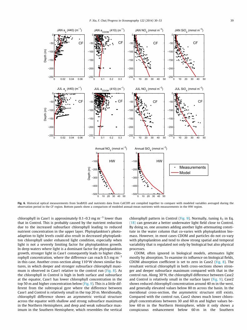
Historical optical measurements from SeaBASS, nutrients datafrom CalCOFI and HOT are compiled together to compare withmodeled variables in the CF and HW regions (Fig. 6). Modeled ni-trate and silicate concentrations fall in the observed ranges, withlow values at the surface and high values at depth. Modeled phy-toplankton absorption shows a subsurface maximum around50 m in both January and July, which is not clearly shown in theSeaBASS dataset that covers both coastal and open oceans but isconsistent with the open-ocean observation in the California Cur-rent System (Millan-Nuñez et al., 1996). Due to strong lightdestruction, modeled CDOM absorption at the surface is consider-ably lower in July than in January. Together with enhanced subsur-face phytoplankton production, it results in a shallower andstronger subsurface CDOM absorption maximum in July. This is

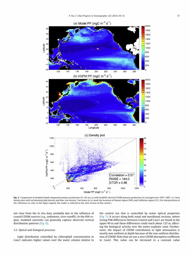
Fig. 3. Comparison of modeled depth-integrated primary production (0–125 m) (a) with SeaWiFS-derived VGPM primary production (b) averaged over 1997–2007. (c): Datadensity plot with red denoting high density and blue, low density. Two boxes in (a) mark the locations of Hawaii region (HW) and California region (CF). (For interpretation ofthe references to color in this figure legend, the reader is referred to the web version of this article.)


not clear from the in situ data, probably due to the influence ofcoastal CDOM sources (e.g., sediments, river runoffs). In the HW re-gion, modeled nutrients can generally capture observed verticaldistribution patterns (Fig. 6).

3.2. Optical and biological processes

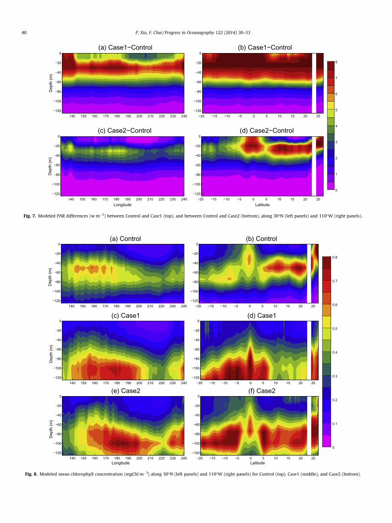
Light distribution controlled by chlorophyll concentration inCase1 indicates higher values over the water column relative to

the control run that is controlled by water optical properties(Fig. 7). It occurs along both zonal and meridional sections, wherestrong PAR differences between Control and Case1 are found in theupper 60 m and these differences could reach about 125 m, affect-ing the biological activity over the entire euphotic zone. Further-more, the impact of CDOM contribution to light attenuation ismostly non-uniform at depth because of the non-uniform distribu-tion of CDOM. Note that we use a zero CDOM absorption coefficientin Case2. This value can be increased to a constant value

97 98 99 00 01 02 03 04 05 06 070

200

400

600

800

1000

HW

97 98 99 00 01 02 03 04 05 06 070

200400600800

1000120014001600

Year

Prim

ary

Prod

uctio

n (m

gC m

−2d−1

)

CF

in−situ Satellite Model

Fig. 4. Comparison of modeled depth-integrated PP with satellite VGPM product and in situ data in the HW and CF regions.

Fig. 5. Left panels: modeled au(440), aCDOM(410), and bbp(550) averaged over 1997–2007. Middle panels: SeaWiFS QAA derived au(443), aCDOM(412), and bbp(555) averagedover 1997–2007. Right panels: data density plot between model and QAA product with red denoting high density and blue, low density. (For interpretation of the referencesto color in this figure legend, the reader is referred to the web version of this article.)

Table 2Statistical results between modeled au(440), aCDOM(410), bbp(550) and SeaWiFS QAAderived au(443), aCDOM(412), bbp(555) averaged over 1997–2007 (Fig. 5).

Model vs. QAA au (440,443) aCDOM (410,412) bbp (550,555)

R 0.62 0.65 0.53RMSE (m�1) 0.0065 0.017 0.0011STDR 0.69 0.54 1.7Bias (m�1) �3.1 � 10�3 �6.3 � 10�3 �2.7 � 10�5


empirically as in Fujii et al. (2007), which will change the magni-tude or the sign of the PAR difference between Case2 and Controlbut still will not generate the substantial spatial variability shownin Control. This is also true for Case1, because the tunable param-eters (k1 and k2) in Eq. (18) are spatially constant. Therefore, the re-sults shown here mainly illustrate the importance of including adetailed CDOM spatial structure to the underwater optical and bio-logical fields.

After entering the water column, visible and shortwave lightsare attenuated due to the absorption and scattering mostly by phy-toplankton, CDOM, and non-algal particles. The remaining light ateach depth will then serve as the source for phytoplankton’s pho-tosynthetic growth. Inaccurate light attenuation treatment in themodel will likely lead to biased phytoplankton production and sub-sequent carbon export to the deep ocean. Compared with theempirical calculation in Case1, modeled phytoplankton chlorophyllconcentration across 30�N shows a much shallower subsurfacemaximum and a relatively smaller magnitude in both westernand eastern basins, suggesting more light entering deep water be-cause of less attenuation in Case1 (Fig. 8). However, the modeledchlorophyll difference between Control and Case1 shows a non-uniform pattern (Fig. 9). There is little difference in the surfacelayer because of ample light for phytoplankton growth and lowsurface chlorophyll. In the subsurface layer around 40 m, eventhough light in Case1 is stronger than that in Control, modeled

0 0.02 0.04 0.06−250

−200

−150

−100

−50

0

Dep

th (m

)

JAN aφ (440) (m−1)

CF

MeasurementsModel

0 0.1 0.2 0.3−250

−200

−150

−100

−50

0

JAN aCDOM (410) (m−1)

CF

0 10 20 30 40 50−250

−200

−150

−100

−50

0

JAN NO3 (mmol m−3)

CF

0 10 20 30 40 50−250

−200

−150

−100

−50

0

JAN SiO4 (mmol m−3)

CF

0 0.02 0.04 0.06−250

−200

−150

−100

−50

0

JUL aφ (440) (m−1)

Dep

th (m

)

CF

0 0.1 0.2 0.3−250

−200

−150

−100

−50

0

JUL aCDOM (410) (m−1)

CF

0 10 20 30 40 50−250

−200

−150

−100

−50

0

JUL NO3 (mmol m−3)

CF

0 10 20 30 40 50−250

−200

−150

−100

−50

0

JUL SiO4 (mmol m−3)

CF

0 10 20 30 40 50−500

−400

−300

−200

−100

0

Dep

th (m

)

Annual NO3 (mmol m−3)

HW

0 10 20 30 40 50−500

−400

−300

−200

−100

0

Annual SiO4 (mmol m−3)

HW

Fig. 6. Historical optical measurements from SeaBASS and nutrients data from CalCOFI are compiled together to compare with modeled variables averaged during theobservation period in the CF region. Bottom panels show a comparison of modeled annual-mean nutrients with measurements in the HW region.


chlorophyll in Case1 is approximately 0.1–0.3 mg m�3 lower thanthat in Control. This is probably caused by the nutrient reductiondue to the increased subsurface chlorophyll leading to reducednutrient concentration in the upper layer. Phytoplankton’s photo-adaption to light levels could also result in decreased phytoplank-ton chlorophyll under enhanced light condition, especially whenlight is not a severely limiting factor for phytoplankton growth.In deep waters where light is a dominant factor for phytoplanktongrowth, stronger light in Case1 consequently leads to higher chlo-rophyll concentration, where the difference can reach 0.5 mg m�3

in this case. Another cross-section along 110�W shows similar fea-tures, in which deeper and stronger subsurface chlorophyll maxi-mum is observed in Case1 relative to the control run (Fig. 8). Asthe chlorophyll in Control is high in both surface and subsurfaceat the equator, Case1 has lower chlorophyll concentration in thetop 50 m and higher concentration below (Fig. 9). This is a little dif-ferent from the subtropical gyre where the difference betweenCase1 and Control is relatively small in the top 20 m. Meridionally,chlorophyll difference shows an asymmetric vertical structureacross the equator with shallow and strong subsurface maximumin the Northern Hemisphere, and deep and weak subsurface max-imum in the Southern Hemisphere, which resembles the vertical

chlorophyll pattern in Control (Fig. 9). Normally, tuning k2 in Eq.(18) can generate a better underwater light field close to Control.By doing so, one assumes adding another light-attenuating consti-tute in the water column that co-varies with phytoplankton bio-mass. However, in most cases CDOM and particles do not co-varywith phytoplankton and tend to show strong spatial and temporalvariability that is regulated not only by biological but also physicalprocesses.

CDOM, often ignored in biological models, attenuates lightmostly by absorption. To examine its influence on biological fields,CDOM absorption coefficient is set to zero in Case2 (Fig. 8). Theresultant vertical chlorophyll in both cross-sections shows stron-ger and deeper subsurface maximum compared with that in thecontrol run. Along 30�N, the chlorophyll difference between Case2and Control is relatively small in the surface layer (Fig. 9). Case2shows reduced chlorophyll concentration around 40 m in the west,and generally elevated values below 80 m across the basin. In themeridional cross-section, the asymmetric structure still exists.Compared with the control run, Case2 shows much lower chloro-phyll concentrations between 30 and 60 m and higher values be-low 60 m in the Northern Hemisphere, while it only shows aconspicuous enhancement below 60 m in the Southern

Dep

th (m

)(a) Case1−Control

140 150 160 170 180 190 200 210 220 230 240−120

−100

−80

−60

−40

−20

0D

epth

(m)

(c) Case2−Control

Longitude140 150 160 170 180 190 200 210 220 230 240

−120

−100

−80

−60

−40

−20

0

(b) Case1−Control

−20 −15 −10 −5 0 5 10 15 20 25−120

−100

−80

−60

−40

−20

0

0

1

2

3

4

5

6

7

8

(d) Case2−Control

Latitude−20 −15 −10 −5 0 5 10 15 20 25

−120

−100

−80

−60

−40

−20

0

Fig. 7. Modeled PAR differences (w m�2) between Control and Case1 (top), and between Control and Case2 (bottom), along 30�N (left panels) and 110�W (right panels).

Dep

th (m

)

(a) Control

140 150 160 170 180 190 200 210 220 230 240−120

−100

−80

−60

−40

−20

0

Dep

th (m

)

(c) Case1

140 150 160 170 180 190 200 210 220 230 240−120

−100

−80

−60

−40

−20

0

Dep

th (m

)

Longitude

(e) Case2

140 150 160 170 180 190 200 210 220 230 240−120

−100

−80

−60

−40

−20

0

(b) Control

−20 −15 −10 −5 0 5 10 15 20 25−120

−100

−80

−60

−40

−20

0

(d) Case1

−20 −15 −10 −5 0 5 10 15 20 25−120

−100

−80

−60

−40

−20

0

0

0.1

0.2

0.3

0.4

0.5

0.6

0.7

0.8

Latitude

(f) Case2

−20 −15 −10 −5 0 5 10 15 20 25−120

−100

−80

−60

−40

−20

0

Fig. 8. Modeled mean chlorophyll concentration (mgChl m�3) along 30�N (left panels) and 110�W (right panels) for Control (top), Case1 (middle), and Case2 (bottom).


Dep

th (m

)

(a) Case1−Control

140 150 160 170 180 190 200 210 220 230 240−120

−100

−80

−60

−40

−20

0D

epth

(m)

(c) Case2−Control

Longitude140 150 160 170 180 190 200 210 220 230 240

−120

−100

−80

−60

−40

−20

0

(b) Case1−Control

−20 −15 −10 −5 0 5 10 15 20 25−120

−100

−80

−60

−40

−20

0

−0.5

−0.4

−0.3

−0.2

−0.1

0

0.1

0.2

0.3

0.4

0.5

(d) Case2−Control

Latitude−20 −15 −10 −5 0 5 10 15 20 25

−120

−100

−80

−60

−40

−20

0

Fig. 9. Modeled chlorophyll concentration differences (mgChl m�3) between Control and Case1 (top), and between Control and Case2 (bottom), along 30�N (left panels) and110�W (right panels).

Latit

ude

(a) (Case1−Control)/Control (%)

120 140 160 180 200 220 240 260 280−20

−10

0

10

20

30

40

50

60

−100

−80

−60

−40

−20

0

20

40

60

80

100

Longitude

Latit

ude

(b) (Case2−Control)/Control (%)

120 140 160 180 200 220 240 260 280−20

−10

0

10

20

30

40

50

60

Fig. 10. Percentile differences of modeled depth-integrated PP averaged during 2000–2009 between Control and Case1 (a), and between Control and Case2 (b).


00 01 02 03 04 05 06 07 08 09

0.8

1

1.2

1.4

1.6

Silic

ate

(mm

ol m

−3)

HW

00 01 02 03 04 05 06 07 08 095

10

15

20

25

PAR

(w m

−2)

Year

Control Case1 Case2

Fig. 11. Time series of depth-integrated mean of silicate concentrations and PAR values over the top 125 m in the HW region.


Hemisphere, which implies the importance of the spatial variabil-ity in CDOM distribution to underwater light field that controlsbiological production.

The spatial distribution of the depth-integrated PP differencebetween Control and Case1 indicates that the light treatment inCase1 could lead to primary production 50% higher in the easternequatorial Pacific and North Pacific than in the control run(Fig. 10a). In the subtropical gyre, the PP difference is relativelysmall, about 10% lower in Case1. While in the western equatorialPacific, Case1 appears to have about 25% lower PP than the controlrun. Over the entire basin, the mean PP difference between Case1and Control is about 14%, comparable with the 10% between Case2and Control. Without considering CDOM absorption in Case2,about 33% of the domain area is covered with less than 10% PP dif-ference (Fig. 10b). Relative to Control, higher values of PP (relativedifference >10%) in Case2 possessing about 39% of the total domainarea, occur in the eastern North Pacific, a latitudinal band between15� and 25�N stretching from the Luzon Strait to the Hawaii Is-lands, as well as a patch between 160� and 210�E in the South-ern-Hemisphere subtropical gyre, with the largest differencereaching over 100%. In comparison, about 29% of the domain areais covered with significantly lower PP in Case2 compared with Con-trol (relative difference <�10%), and most of it is located in thewestern basin.

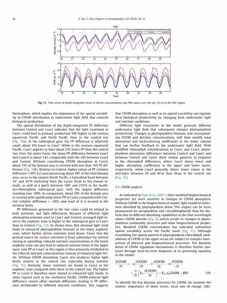
PP differences generated in the two cases could be related toboth nutrients and light differences. Because of different lightattenuation schemes used in Case1 and Control, averaged light le-vel in the euphotic zone is higher in the subtropical gyre in Case1than in Control (Fig. 11). As shown here, this elevated light levelleads to enhanced phytoplankton biomass in the lower euphoticzone, which further drives nutrients level down. Given that thegeneral source for surface nutrients is from subsurface via verticalmixing or upwelling, reduced nutrient concentrations in the lowereuphotic zone can also lead to reduced nutrient levels in the upperlayer. Low PP in Case1 in this region is thus primarily attributed tothe reduced nutrient concentrations instead of enhanced light lev-els. Without CDOM absorption, Case2 also produces higher lightlevels relative to the control run, especially during summer(Fig. 11). Similarly, lower nutrients are found in Case2 in theeuphotic zone compared with those in the control run. The higherPP in Case2 is therefore more related to enhanced light levels. Inother regions such as the northwest Pacific, CDOM-induced lightdifference cannot offset nutrient difference, leading to PP differ-ence attributable to different nutrient conditions. This suggests

that CDOM absorption as well as its spatial variability can regulatelocal biological productivity by changing both underwater lightand nutrient conditions.

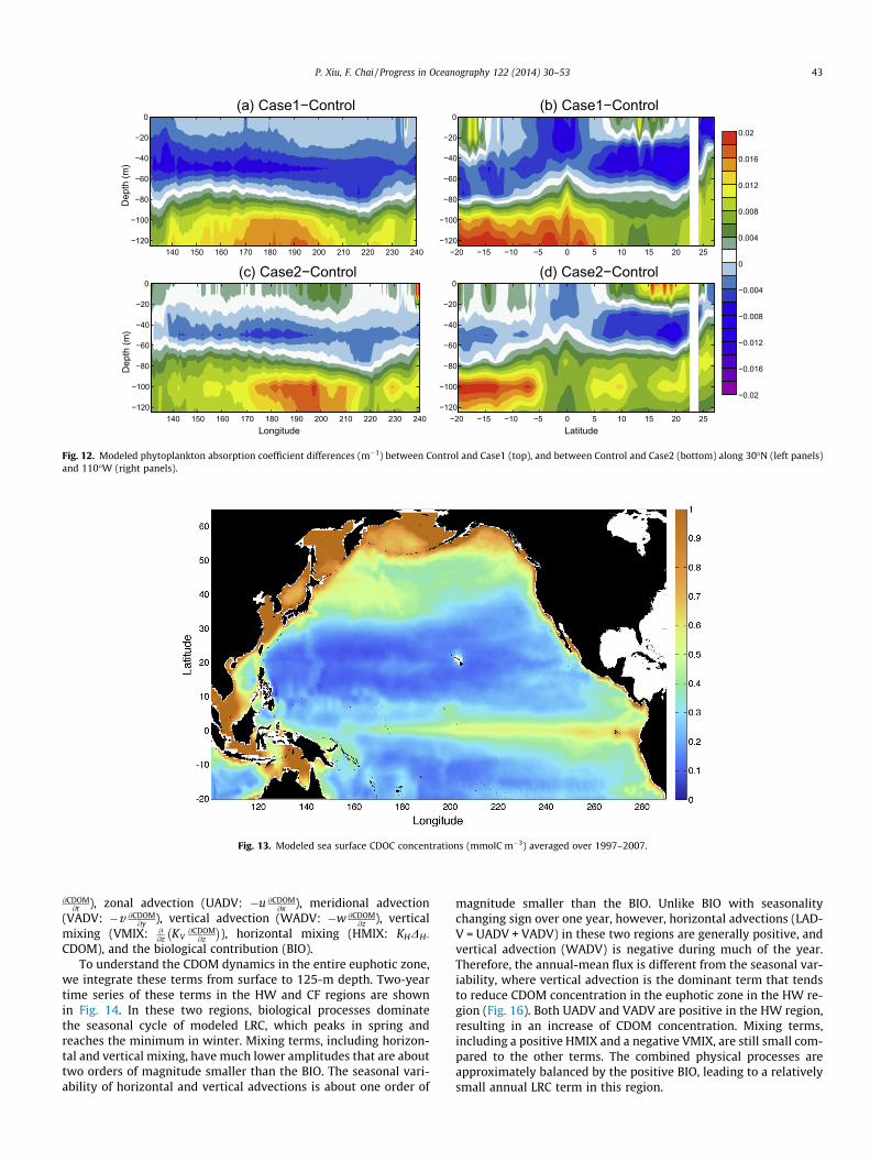
Different light treatments in the model generate differentunderwater light field that subsequent changes phytoplanktonproductivity. Changes in phytoplankton biomass, and correspond-ing CDOM and detritus concentrations, will then modify totalabsorption and backscattering coefficients in the water columnthat can further feedback to the underwater light field. Withmodified chlorophyll concentrations in Case1 and Case2, phyto-plankton absorption differences between Control and Case1 andbetween Control and Case2 show similar patterns in responseto the chlorophyll differences, where Case1 shows lower andhigher absorption coefficients in the upper and lower layers,respectively, while Case2 generally shows lower values in themid-layer between 20 and 60 m than those in the control run(Fig. 12).

3.3. CDOM analysis

As indicated in Fujii et al. (2007), their modeled biogeochemicalproperties are most sensitive to changes in CDOM absorption.Without CDOM in the biogeochemical model, light would be other-wise absorbed by phytoplankton alone. This impact can be morepronounced for picoplankton and coccolithophorids than for dia-toms due to different absorbing capabilities in the blue wavelengthwhere CDOM absorbs (Fig. 2), which results in changes in phyto-plankton community structure and other biogeochemical proper-ties. Modeled CDOM concentration has indicated substantialspatial variability across the Pacific basin (Fig. 13). Althoughresembling the spatial pattern of phytoplankton chlorophyll, mod-ulations of CDOM in the upper ocean are subject to complex inter-actions of physical and biogeochemical processes. The dynamicdetail of CDOM regulation mechanisms is therefore further ana-lyzed through term-by-term diagnosis of its governing equationin the model:

@CDOM@t

¼ �u@CDOM@x

� v @CDOM@y

�w@CDOM@z

þ @

@zKV

@CDOM@z

� �þ KHDHCDOMþ BIO: ð19Þ

To identify the key dynamic processes for CDOM, we examine therelative importance of these terms: local rate of change (LRC:

Dep

th (m

)

(a) Case1−Control

140 150 160 170 180 190 200 210 220 230 240−120

−100

−80

−60

−40

−20

0D

epth

(m)

(c) Case2−Control

Longitude140 150 160 170 180 190 200 210 220 230 240

−120

−100

−80

−60

−40

−20

0

(b) Case1−Control

−20 −15 −10 −5 0 5 10 15 20 25−120

−100

−80

−60

−40

−20

0

−0.02

−0.016

−0.012

−0.008

−0.004

0

0.004

0.008

0.012

0.016

0.02

(d) Case2−Control

Latitude−20 −15 −10 −5 0 5 10 15 20 25

−120

−100

−80

−60

−40

−20

0

Fig. 12. Modeled phytoplankton absorption coefficient differences (m�1) between Control and Case1 (top), and between Control and Case2 (bottom) along 30�N (left panels)and 110�W (right panels).

Fig. 13. Modeled sea surface CDOC concentrations (mmolC m�3) averaged over 1997–2007.


@CDOM@t ), zonal advection (UADV: �u @CDOM

@x ), meridional advection(VADV: �v @CDOM

@y ), vertical advection (WADV: �w @CDOM@z ), vertical

mixing (VMIX: @@z KV

@CDOM@z

� �), horizontal mixing (HMIX: KHDH-

CDOM), and the biological contribution (BIO).To understand the CDOM dynamics in the entire euphotic zone,

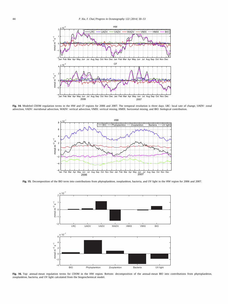
we integrate these terms from surface to 125-m depth. Two-yeartime series of these terms in the HW and CF regions are shownin Fig. 14. In these two regions, biological processes dominatethe seasonal cycle of modeled LRC, which peaks in spring andreaches the minimum in winter. Mixing terms, including horizon-tal and vertical mixing, have much lower amplitudes that are abouttwo orders of magnitude smaller than the BIO. The seasonal vari-ability of horizontal and vertical advections is about one order of

magnitude smaller than the BIO. Unlike BIO with seasonalitychanging sign over one year, however, horizontal advections (LAD-V = UADV + VADV) in these two regions are generally positive, andvertical advection (WADV) is negative during much of the year.Therefore, the annual-mean flux is different from the seasonal var-iability, where vertical advection is the dominant term that tendsto reduce CDOM concentration in the euphotic zone in the HW re-gion (Fig. 16). Both UADV and VADV are positive in the HW region,resulting in an increase of CDOM concentration. Mixing terms,including a positive HMIX and a negative VMIX, are still small com-pared to the other terms. The combined physical processes areapproximately balanced by the positive BIO, leading to a relativelysmall annual LRC term in this region.

Jan Feb Mar Apr May Jun Jul Aug Sep Oct Nov Dec Jan Feb Mar Apr May Jun Jul Aug Sep Oct Nov Dec−2

−1

0

1

2x 10−6

mm

ol m

−2 s

−1

HW

LRC UADV VADV WADV VMIX HMIX BIO


−2

0

2

4x 10−6

mm

ol m

−2 s

−1

CF

2006 2007

Fig. 14. Modeled CDOM regulation terms in the HW and CF regions for 2006 and 2007. The temporal resolution is three days. LRC: local rate of change, UADV: zonaladvection, VADV: meridional advection, WADV: vertical advection, VMIX: vertical mixing, HMIX: horizontal mixing, and BIO: biological contribution.


−4

−2

0

2

4

6

8 x 10−7 HW

mm

ol m

−2 s

−1

2006 2007

BIO Phytoplankton Zooplankton Bacteria UV light

Fig. 15. Decomposition of the BIO term into contributions from phytoplankton, zooplankton, bacteria, and UV light in the HW region for 2006 and 2007.

LRC UADV VADV WADV HMIX VMIX BIO−2

−1

0

1

2x 10−7

mm

ol m

−2 s

−1

BIO Phytoplankton Zooplankton Bacteria UV light−4

−2

0

2

4

6x 10−7

mm

ol m

−2 s

−1

Fig. 16. Top: annual-mean regulation terms for CDOM in the HW region. Bottom: decomposition of the annual-mean BIO into contributions from phytoplankton,zooplankton, bacteria, and UV light calculated from the biogeochemical model.


−1e−08

−8e−09

−6e−09

−4e−09

−2e−09

0

2e−09

4e−09

6e−09

8e−09

1e−08 UADV+VADV

Dep

th (m

)

140 160 180 200 220 240−120

−100

−80

−60

−40

−20

0

−1e−08

−8e−09

−6e−09

−4e−09

−2e−09

0

2e−09

4e−09

6e−09

8e−09

1e−08 WADV

Dep

th (m

)

140 160 180 200 220 240−120

−100

−80

−60

−40

−20

0

−1e−08

−8e−09

−6e−09

−4e−09

−2e−09

0

2e−09

4e−09

6e−09

8e−09

1e−08 BIO

Longitude

Dep

th (m

)

140 160 180 200 220 240−120

−100

−80

−60

−40

−20

0

Fig. 17. Sections along 30�N depicting the vertical structures of annual-mean advection and biology terms contributing to CDOM dynamics.


In the biogeochemical model, the BIO is determined by sourceand sink terms. The source terms include phytoplankton excretionand zooplankton feeding loss, and the sink terms are composed ofbacteria uptake and photolysis by UV light. For the entire euphoticzone in the HW region, seasonal variation of the BIO follows closelywith change in phytoplankton excretion, and in bacteria uptakewith seasonal peaks between spring and summer (Fig. 15). Zoo-plankton feeding loss and photolysis stay relatively constant overthe two-year period. When averaged over time, two dominantterms in the annual-mean BIO are phytoplankton excretion andbacteria uptake that are significantly higher than the contributionsfrom zooplankton feeding loss and photolysis, as UV light is intensemostly in the upper layer, while bacteria uptake generally takesplace throughout the euphotic zone (Fig. 16).

The zonal transection along 30�N further depicts the verticalstructures of the annual-mean terms contributing to the CDOMdynamics (Fig. 17). Both horizontal and vertical advections, as wellas the BIO term, are considerably stronger in the coastal regionsrelative to the central basin. Horizontal advections are shown tobe highly variable in both horizontal and vertical directions, whilevertical advection shows a relatively coherent feature with nega-tive values above 70 m and positive values below, except for theregion around 140�W where negative values exist in the entire

euphotic zone. Due to the photolysis by UV light, the BIO termillustrates large negative values in the upper layer and varies indepth across the transection. Away from the surface layer, negativeBIO values, especially those generally found at the bottom of theeuphotic zone, are primarily attributable to bacteria uptake. Onthe other hand, the BIO source terms, including phytoplanktonand zooplankton contributions, are more distinct in the middle ofthe euphotic zone with clear spatial variability across this transec-tion. This suggests CDOM dynamics are highly variable in space,which is induced by the variability in both physical and biologicalprocesses.

Physical process affecting biological properties such as phyto-plankton chlorophyll via (horizontal and vertical) transports ofnutrients, and sometimes the chlorophyll itself, has been widely ac-cepted as the concept of how physics changes biology in the ocean.However, when considering ocean optics, another mechanism be-comes possible: physical transport of CDOM changes water opticalproperties, which can further modify underwater light field andsubsequently affect phytoplankton chlorophyll. Positive transportof CDOM can increase water optical properties, increase light atten-uation, decrease underwater PAR values, and eventually decreaselocal chlorophyll concentration. This mechanism is different fromthe one where positive transport of nutrients or chlorophyll usually

−1

−0.95

−0.9

−0.85

−0.8

−0.75

−0.7

−0.65

−0.6

−0.55

−0.5

−0.45

−0.4

−0.35

−0.3 Control

Latit

ude

120 140 160 180 200 220 240 260 280−20

−10

0

10

20

30

40

50

60

−1

−0.95

−0.9

−0.85

−0.8

−0.75

−0.7

−0.65

−0.6

−0.55

−0.5

−0.45

−0.4

−0.35

−0.3 Case1

Longitude

Latit

ude

120 140 160 180 200 220 240 260 280−20

−10

0

10

20

30

40

50

60

Fig. 18. Correlation coefficients between horizontal advection term (LADV) and BIO term for CDOM dynamics using two-year time series (2006 and 2007) for Control andCase1. A two-week high-frequency-pass filter was applied prior to the correlation calculation.


leads to an increase of local biomass. To illustrate this mechanism,correlation coefficients between horizontal advection term (LADV)and BIO term for CDOM are calculated (Fig. 18). As the BIO tends todominate the seasonal cycle of the local CDOM concentration, atwo-week high-frequency-pass filter is applied for the horizontaladvection and BIO before the correlation is calculated. In Case1where light is only controlled by phytoplankton, advection ofCDOM does not change underwater PAR and subsequent BIOCDOM. However, there is still significant negative correlation be-tween LADV and BIO in the equatorial Pacific and most of the NorthPacific. This is likely related to the photolysis by UV light in the BIOcalculation, in which positive LADV CDOM increases local CDOMconcentration that can increase photolysis and consequently de-crease BIO CDOM. In the control run where light attenuation byCDOM is considered, the correlation coefficient between LADVand BIO systematically increases compared to that in Case1, espe-cially in the subtropics where the correlation is not significant inCase1. This high negative correlation generally presents over theentire basin, implying optical modulation of physical–biologicalinteractions. Without explicitly representing CDOM dynamics inthe biogeochemical model, this effect is often ignored by manystudies. Here, we only show the influence of physical transport ofCDOM on biological process, as we do not include its biological

feedback to physical properties in the model. If we considered thisfeedback, we could expect the modification of water temperatureby physical transport of CDOM, because LADV of CDOM can changeboth underwater PAR (400–700 nm) and shortwave radiation (usu-ally in 400–1000 nm) that heats the upper ocean.

4. Discussion and conclusions

Satellite-observed CDOM generally shows different spatial dis-tribution patterns from chlorophyll, attributable to distinct sourceand sink processes (Nelson and Siegel, 2013). This creates estima-tion errors for empirical chlorophyll retrieval algorithms, sayOC4V4, which assumes a fixed relationship between chlorophylland CDOM concentrations. These errors, without proper con-straints, could manifest in the assessment of ocean carbon cycling.For example, Siegel et al. (2005) calculated a global net primaryproduction of 53.5 Gt C y�1 based on OC4V4-derived chlorophyllconcentration; this number is reduced to 37.1 Gt C y�1 when usingthe chlorophyll concentration from a semi-analytical algorithmbased on independent CDOM calculations. With different chloro-phyll retrieval algorithms, the discrepancy between these calcula-tions is uncertain, but it suggests that the potential impact ofCDOM on ecosystem processes and functions may not be trivial.


As indicated by Siegel et al. (2005), without accurately separatingin-water constituents, interpretations of ocean color data (e.g., sea-sonal analysis, trend detection) could be easily confounded byuncertainties, especially due to the nonlinear relationship betweenCDOM and chlorophyll. Our study confirms that CDOM dynamicsshould be explicitly considered in biogeochemical models, as itcan feed back to the whole marine system including physics, op-tics, and biogeochemistry.

Currently, coupled ecosystem models typically use sophisti-cated thermodynamics, fairly sophisticated biology, but grosslysimplified underwater light attenuation. Models used for global-scale predictions of climate change as well as for understandingthe global ocean–atmosphere system are often driven by simpleanalytical formulations of light penetration through the water col-umn. A lot of efforts have been made to improve model resolutionand the dynamics of physical and biological model components. Incontrast, the uncertainty induced by the oversimplified treatmentof light has rarely been discussed. The difference between Controland Case1 suggests that this uncertainty cannot be ignored. It notonly changes underwater light condition but also alters distribu-tions of phytoplankton chlorophyll and nutrient levels, and tendsto be more significant in the subsurface, which could potentiallyaffect the efficiency and structure of the biological pump and car-bon cycling.

To summarize, a new biogeochemical model consisting of 31state variables has been developed and coupled to a 3-D physicalmodel in the Pacific Ocean. With the explicitly represented DOMpool, this new model is able to link key biogeochemical processeswith optical processes. Moreover, the inclusion of optical processesallows direct comparison between model and satellite-derivedoptical data, which gives additional constraints on model parame-ters to reduce uncertainties in model simulations. The develop-ment of this new model and parameter tuning rely on variousmodeling approaches, such as phytoplankton photoacclimation,CDOM dynamics, microbial loop, optics conversion, among others,based on previous studies (e.g., Anderson and Williams, 1998;Geider et al., 1998; Bissett et al., 1999a; Chai et al., 2002; Mooreet al., 2002;Fujii et al., 2007). In practice, it is difficult to modelan entire ocean basin with a wide range of biological provincesand diverse phytoplankton communities using only one set ofmodel parameters. Nevertheless, model validation against satelliteand in situ data appears to show that the model is flexible enoughto reproduce general biogeochemical and optical featuresobserved.

The main advantage of the coupled model is that it combinesphysical, biogeochemical, and optical processes. Our results dem-onstrate the importance of CDOM in regulating underwater lightfield and subsequent biological activities. Our analysis suggeststhat the inclusion of CDOM in the ecosystem model could substan-tially affect biological processes. Without CDOM attenuating light,modeled depth-integrated PP is about 10% higher than that in thecontrol run over the entire Pacific basin. Moreover, this discrep-ancy is highly variable in space with magnitudes reaching higherthan 100% in some locations. The coupled model demonstrates thatthe physical transport of CDOM can change water optical proper-ties, which can further modify underwater light field and subse-quently affect the distribution of phytoplankton chlorophyll. Thismechanism is different from the one where transport of nutrientsand/or chlorophyll usually leads to an increase of local biomass.One potential for this coupled model is to assimilate satellite-sensed or in situ optical data directly in addition to chlorophyllconcentration. This will increase the realism of ecosystem simula-tions for better prediction and monitoring of biological conditions(e.g., harmful algal blooms) in open oceans and coastal regions.

Acknowledgements

This research was supported by NASA grants (NNG04GM64Gand NNX09AU39G) to F. Chai. The authors wish to thank the SeaW-iFS Project for providing the SeaWiFS data (http://oceancol-or.gsfc.nasa.gov/), and the editor and three anonymous reviewersfor their valuable comments.

Appendix A

A.1. Governing equations

The model equations describing individual compartments alltake the form:

@Bi

@t¼ PHYðBiÞ þ BIOðBiÞ: ðA1Þ

The model state variables, Bi, represent picoplankton (P1(mmolN m�3), C1 (mmolC m�3), and Chl1 (mgChl m�3)), diatoms(P2 (mmolN m�3), C2 (mmolC m�3), and Chl2 (mgChl m�3)), cocco-lithophorids (P3 (mmolN m�3), C3 (mmolC m�3), and Chl3(mgChl m�3)), microzooplankton (Z1 (mmolN m�3), ZC1(mmolC m�3)), mesozooplankton (Z2 (mmolN m�3), ZC2(mmolC m�3)), bacteria nitrogen (BAC (mmolN m�3)), detritus(PON (mmolN m�3), POC (mmolC m�3)), biogenic silicate (bSiO2

(mmolSi m�3)), calcium carbonate (PIC (mmolC m�3)), labile DON(LDON (mmolN m�3)), labile DOC (LDOC (mmolC m�3)), semi-labileDON (SDON (mmolN m�3)), semi-labile DOC (SDOC (mmolC m�3)),colored labile DOC (CLDOC (mmolC m�3)), colored semi-labileDOC (CSDOC (mmolC m�3)), dissolved oxygen (DO (mmolO m�3)),dissolved inorganic nutrients (NO3 (mmolN m�3), NH4

(mmolN m�3), PO4 (mmolP m�3), SiO4 (mmolSi m�3)), total alkalin-ity (TALK (mmol m�3)), and total CO2 (TCO2 (mmolC m�3)).

The term PHY(Bi) represents the contribution to concentrationchange due to physical processes. The term BIO(Bi) represents bio-logical sources and sinks of a particular compartment. The BIO(Bi)terms in the model are:

BIOðP1Þ ¼ ð1� e1ÞPP1|fflfflfflfflfflfflfflfflffl{zfflfflfflfflfflfflfflfflffl}growth

� G1|{z}grazing by Z1

� c3P1|ffl{zffl}mortality

; ðA2Þ

BIOðC1Þ ¼ ð1� e1ÞNPC1|fflfflfflfflfflfflfflfflfflfflffl{zfflfflfflfflfflfflfflfflfflfflffl}growth

� G1 �C1P1|fflfflfflfflffl{zfflfflfflfflffl}

grazing by Z1

� c3C1|ffl{zffl}mortality

; ðA3Þ

BIOðChl1Þ ¼ qChl1ð1� e1ÞPP1|fflfflfflfflfflfflfflfflfflfflfflfflfflffl{zfflfflfflfflfflfflfflfflfflfflfflfflfflffl}growth

�G1 �Chl1P1|fflfflfflfflfflfflffl{zfflfflfflfflfflfflffl}

grazing by Z1

� c3Chl1|fflfflfflffl{zfflfflfflffl}mortality

; ðA4Þ



� c4P2|ffl{zffl}mortality

� @

@zðW1P2Þ|fflfflfflfflfflfflffl{zfflfflfflfflfflfflffl}sin king

; ðA5Þ



grazing by Z2

� c4C2|ffl{zffl}mortality

� @

@zðW1C2Þ|fflfflfflfflfflfflffl{zfflfflfflfflfflfflffl}sin king

; ðA6Þ

BIOðChl2Þ¼qChl2ð1�e2ÞPP2|fflfflfflfflfflfflfflfflfflfflfflfflffl{zfflfflfflfflfflfflfflfflfflfflfflfflffl}growth

�G2ðzÞ�Chl2P2|fflfflfflfflfflfflfflfflffl{zfflfflfflfflfflfflfflfflffl}

grazing by Z2

�c4Chl2|fflfflfflffl{zfflfflfflffl}mortality

� @

@zðW1Chl2Þ|fflfflfflfflfflfflfflfflffl{zfflfflfflfflfflfflfflfflffl}

sinking

;

ðA7Þ



� c10P3|fflffl{zfflffl}mortality

� @

@zðW3P3Þ|fflfflfflfflfflfflffl{zfflfflfflfflfflfflffl}sin king

; ðA8Þ

http://oceancolor.gsfc.nasa.gov/

http://oceancolor.gsfc.nasa.gov/




grazing by Z2

� c10C3|fflffl{zfflffl}mortality

� @

@zðW3C3Þ|fflfflfflfflfflfflffl{zfflfflfflfflfflfflffl}sin king

; ðA9Þ

BIOðChl3Þ ¼ qChl3ð1� e3ÞPP3|fflfflfflfflfflfflfflfflfflfflfflfflffl{zfflfflfflfflfflfflfflfflfflfflfflfflffl}growth

�G5 �Chl3P3|fflfflfflfflfflfflffl{zfflfflfflfflfflfflffl}

grazing by Z2

� c10Chl3|fflfflfflffl{zfflfflfflffl}mortality

� @

@zðW3Chl3Þ|fflfflfflfflfflfflfflfflfflffl{zfflfflfflfflfflfflfflfflfflffl}

sin king

;

ðA10Þ

BIOðZ1Þ ¼ c1ð1� /1ÞðG1 þ G6Þ|fflfflfflfflfflfflfflfflfflfflfflfflfflfflfflfflffl{zfflfflfflfflfflfflfflfflfflfflfflfflfflfflfflfflffl}grazing

� G3|{z}predation by Z2

� reg1Z1|fflfflffl{zfflfflffl}excretion

; ðA11Þ

BIOðZC1Þ ¼ c1ð1� /1Þ G1C1P1þ RBG6

� �|fflfflfflfflfflfflfflfflfflfflfflfflfflfflfflfflfflfflfflfflfflfflfflfflffl{zfflfflfflfflfflfflfflfflfflfflfflfflfflfflfflfflfflfflfflfflfflfflfflfflffl}

grazing

� G3ZC1Z1|fflfflffl{zfflfflffl}

predation by Z2

� reg1ZC1|fflfflfflfflffl{zfflfflfflfflffl}excretion

;

ðA12Þ

BIOðZ2Þ ¼ c2ð1� /2ÞðG2 þ G3 þ G4 þ G5Þ|fflfflfflfflfflfflfflfflfflfflfflfflfflfflfflfflfflfflfflfflfflfflfflfflfflfflfflffl{zfflfflfflfflfflfflfflfflfflfflfflfflfflfflfflfflfflfflfflfflfflfflfflfflfflfflfflffl}grazing

� reg2Z2|fflfflffl{zfflfflffl}excretion

� kZ22|ffl{zffl}loss

; ðA13Þ

BIOðZC2Þ ¼ c22ð1� /2Þ G2C2P2þ G3

ZC1Z1þ G4

POCPON

þ G5C3P3

� �|fflfflfflfflfflfflfflfflfflfflfflfflfflfflfflfflfflfflfflfflfflfflfflfflfflfflfflfflfflfflfflfflfflfflfflfflfflfflfflfflfflfflfflfflfflfflffl{zfflfflfflfflfflfflfflfflfflfflfflfflfflfflfflfflfflfflfflfflfflfflfflfflfflfflfflfflfflfflfflfflfflfflfflfflfflfflfflfflfflfflfflfflfflfflffl}

grazing

� reg2ZC2|fflfflfflfflffl{zfflfflfflfflffl}excretion

� kZC22|fflfflffl{zfflfflffl}loss

; ðA14Þ

BIOðNH4Þ ¼ � RP1|{z}uptake by P1

� RP2|{z}uptake by P2

� RP3|{z}uptake by P3

þ reg1Z1þ reg2Z2|fflfflfflfflfflfflfflfflfflfflfflfflfflffl{zfflfflfflfflfflfflfflfflfflfflfflfflfflffl}Z1; Z2 excretion

þ 0:9DPONPON|fflfflfflfflfflfflfflfflffl{zfflfflfflfflfflfflfflfflffl}PON re min eralization

� c7NH4|fflfflffl{zfflfflffl}nitrification

þ EB|{z}BAC re min eralization

; ðA15Þ

BIOðSiO4Þ ¼ � USiO4|fflfflffl{zfflfflffl}silicification

þ DSi � bSiO2|fflfflfflfflfflfflfflffl{zfflfflfflfflfflfflfflffl}re min eralization

; ðA16Þ

BIOðNO3Þ ¼ � NP1|ffl{zffl}uptake by P1

� NP2|ffl{zffl}uptake by P2

� NP3|ffl{zffl}uptake by P3

þ c7NH4|fflfflffl{zfflfflffl}nitrification

; ðA17Þ

BIOðPO4Þ ¼ RPN �PP1� PP2� PP3|fflfflfflfflfflfflfflfflfflfflfflfflfflffl{zfflfflfflfflfflfflfflfflfflfflfflfflfflffl}uptake by phytoplankton

þ reg1Z1þ reg2Z2|fflfflfflfflfflfflfflfflfflfflfflfflfflffl{zfflfflfflfflfflfflfflfflfflfflfflfflfflffl}Z1; Z2 excretion

0B@

þ 0:9DPONPON|fflfflfflfflfflfflfflfflffl{zfflfflfflfflfflfflfflfflffl}PON re min eralization


1A; ðA18Þ

BIOðbSiO2Þ ¼ Si2N� G2|{z}fecal pellet

þ c4P2|ffl{zffl}P2 mortality

0B@

1CA� DSi � bSiO2|fflfflfflfflfflfflfflffl{zfflfflfflfflfflfflfflffl}

re min eralization

� @

@zðW4bSiO2Þ|fflfflfflfflfflfflfflfflfflfflffl{zfflfflfflfflfflfflfflfflfflfflffl}

sin king

; ðA19Þ

BIOðPICÞ ¼ RCaC G5C3P3|fflffl{zfflffl}

fecal pellet

þ c10C3|fflffl{zfflffl}P3 mortality

0BB@

1CCA� DPICPIC|fflfflfflffl{zfflfflfflffl}

dissolution

� @

@zðW5PICÞ|fflfflfflfflfflfflfflffl{zfflfflfflfflfflfflfflffl}sin king

;

ðA20Þ

BIOðPONÞ ¼ ð1� c2Þð1� /2ÞðG2 þ G3 þ G4 þ G5Þ|fflfflfflfflfflfflfflfflfflfflfflfflfflfflfflfflfflfflfflfflfflfflfflfflfflfflfflfflfflfflfflfflfflfflffl{zfflfflfflfflfflfflfflfflfflfflfflfflfflfflfflfflfflfflfflfflfflfflfflfflfflfflfflfflfflfflfflfflfflfflffl}fecal pellet by Z2

þ ð1� c1Þð1� /1ÞðG1 þ G6Þ|fflfflfflfflfflfflfflfflfflfflfflfflfflfflfflfflfflfflfflfflfflfflfflffl{zfflfflfflfflfflfflfflfflfflfflfflfflfflfflfflfflfflfflfflfflfflfflfflffl}fecal pellet by Z1

� G4|{z}Z2 grazing

þ c3ð1� d1ÞP1|fflfflfflfflfflfflfflfflfflffl{zfflfflfflfflfflfflfflfflfflffl}P1 mortality

þ c4ð1� d2ÞP2|fflfflfflfflfflfflfflfflfflffl{zfflfflfflfflfflfflfflfflfflffl}P2 mortality

þ c10ð1� d3ÞP3|fflfflfflfflfflfflfflfflfflfflffl{zfflfflfflfflfflfflfflfflfflfflffl}P3 mortality

� 0:9DPONPON|fflfflfflfflfflfflfflfflffl{zfflfflfflfflfflfflfflfflffl}re min eralization

� 0:1DPONPON|fflfflfflfflfflfflfflfflffl{zfflfflfflfflfflfflfflfflffl}det ritus breakdown

� @

@zðW6PONÞ|fflfflfflfflfflfflfflfflffl{zfflfflfflfflfflfflfflfflffl}

sin king

; ðA21Þ

BIOðPOCÞ ¼ ð1� c22Þð1� /2Þ G2C2P2þ G3

ZC1Z1þ G4

POCPON

þ G5C3P3

� �|fflfflfflfflfflfflfflfflfflfflfflfflfflfflfflfflfflfflfflfflfflfflfflfflfflfflfflfflfflfflfflfflfflfflfflfflfflfflfflfflfflfflfflfflfflfflfflfflfflfflfflfflfflffl{zfflfflfflfflfflfflfflfflfflfflfflfflfflfflfflfflfflfflfflfflfflfflfflfflfflfflfflfflfflfflfflfflfflfflfflfflfflfflfflfflfflfflfflfflfflfflfflfflfflfflfflfflfflffl}

fecal pellet by Z2

þ ð1� c1Þð1� /1Þ G1C1P1þ RBG6

� �|fflfflfflfflfflfflfflfflfflfflfflfflfflfflfflfflfflfflfflfflfflfflfflfflfflfflfflfflfflfflffl{zfflfflfflfflfflfflfflfflfflfflfflfflfflfflfflfflfflfflfflfflfflfflfflfflfflfflfflfflfflfflffl}

fecal pellet by Z1

� G4ðzÞPOCPON|fflfflfflfflfflfflffl{zfflfflfflfflfflfflffl}

grazing by Z2

þ c3ð1� d1ÞC1|fflfflfflfflfflfflfflfflfflffl{zfflfflfflfflfflfflfflfflfflffl}P1 mortality

þ c4ð1� d2ÞC2|fflfflfflfflfflfflfflfflfflffl{zfflfflfflfflfflfflfflfflfflffl}P2 mortality

þ c10ð1� d3ÞC3|fflfflfflfflfflfflfflfflfflfflffl{zfflfflfflfflfflfflfflfflfflfflffl}P3 mortality

� 0:9DPONPOC|fflfflfflfflfflfflfflfflffl{zfflfflfflfflfflfflfflfflffl}POC re min eralization

� 0:1DPONPOC|fflfflfflfflfflfflfflfflffl{zfflfflfflfflfflfflfflfflffl}det ritus breakdown

� @

@zðW7POCÞ|fflfflfflfflfflfflfflfflffl{zfflfflfflfflfflfflfflfflffl}

sin king

;

ðA22Þ

BIOðLDONÞ ¼ e1PP1þ e2PP2þ e3PP3|fflfflfflfflfflfflfflfflfflfflfflfflfflfflfflfflfflfflfflfflffl{zfflfflfflfflfflfflfflfflfflfflfflfflfflfflfflfflfflfflfflfflffl}phytoplankton exudation

þ b1 /1ðG1 þ G6Þ þ /2ðG2 þ G3 þ G4 þ G5Þ|fflfflfflfflfflfflfflfflfflfflfflfflfflfflfflfflfflfflfflfflfflfflfflfflfflfflfflfflfflfflfflfflfflfflfflffl{zfflfflfflfflfflfflfflfflfflfflfflfflfflfflfflfflfflfflfflfflfflfflfflfflfflfflfflfflfflfflfflfflfflfflfflffl}zooplankton messy feeding

264

þ d1c3P1þ d2c4P2þ d3c10P3|fflfflfflfflfflfflfflfflfflfflfflfflfflfflfflfflfflfflfflfflfflfflfflfflffl{zfflfflfflfflfflfflfflfflfflfflfflfflfflfflfflfflfflfflfflfflfflfflfflfflffl}phytoplankton mortality

þ c12BAC|fflfflfflffl{zfflfflfflffl}bacteria mortality

þ 0:1DPONPON|fflfflfflfflfflfflfflfflffl{zfflfflfflfflfflfflfflfflffl}det ritus breakdown

35� UN|{z}

bacteria uptake

þ c13BAC� SDON

KSDON þ SDON|fflfflfflfflfflfflfflfflfflfflfflfflfflfflffl{zfflfflfflfflfflfflfflfflfflfflfflfflfflfflffl}breakdown of SDON

;

ðA23Þ

BIOðSDONÞ ¼ ð1� b1Þ½/1ðG1 þ G6Þ þ /2ðG2 þ G3 þ G4 þ G5Þ|fflfflfflfflfflfflfflfflfflfflfflfflfflfflfflfflfflfflfflfflfflfflfflfflfflfflfflfflfflfflfflfflfflfflfflfflfflfflfflfflfflfflfflfflffl{zfflfflfflfflfflfflfflfflfflfflfflfflfflfflfflfflfflfflfflfflfflfflfflfflfflfflfflfflfflfflfflfflfflfflfflfflfflfflfflfflfflfflfflfflffl}zooplankton messy feeding

þ d1c3P1þ d2c4P2þ d3c10P3|fflfflfflfflfflfflfflfflfflfflfflfflfflfflfflfflfflfflfflfflfflfflfflfflffl{zfflfflfflfflfflfflfflfflfflfflfflfflfflfflfflfflfflfflfflfflfflfflfflfflffl}phytoplankton mortality

þ c12BAC|fflfflfflffl{zfflfflfflffl}bacteria mortality

þ 0:1DPONPON|fflfflfflfflfflfflfflfflffl{zfflfflfflfflfflfflfflfflffl}det ritus breakdown

� � c13BAC� SDON

KSDON þ SDON|fflfflfflfflfflfflfflfflfflfflfflfflfflfflffl{zfflfflfflfflfflfflfflfflfflfflfflfflfflfflffl}breakdown of SDON

; ðA24Þ

BIOðLDOCÞ ¼ ð1� colorFR1Þ½e1ð1� e4ÞNPC1þ e2ð1� e5ÞNPC2þ e3ð1� e6ÞNPC3|fflfflfflfflfflfflfflfflfflfflfflfflfflfflfflfflfflfflfflfflfflfflfflfflfflfflfflfflfflfflfflfflfflfflfflfflfflfflfflfflfflfflfflfflfflfflfflfflfflfflfflfflfflfflfflfflfflfflfflfflfflfflfflfflfflffl{zfflfflfflfflfflfflfflfflfflfflfflfflfflfflfflfflfflfflfflfflfflfflfflfflfflfflfflfflfflfflfflfflfflfflfflfflfflfflfflfflfflfflfflfflfflfflfflfflfflfflfflfflfflfflfflfflfflfflfflfflfflfflfflfflfflffl}þphytoplankton exudation

b1

/1 G1C1P1þRBG6

� �þ/2 G2

C2P2þG3

ZC1Z1þG4

POCPON

þG5C3P3

� �� |fflfflfflfflfflfflfflfflfflfflfflfflfflfflfflfflfflfflfflfflfflfflfflfflfflfflfflfflfflfflfflfflfflfflfflfflfflfflfflfflfflfflfflfflfflfflfflfflfflfflfflfflfflfflfflfflfflfflfflfflfflffl{zfflfflfflfflfflfflfflfflfflfflfflfflfflfflfflfflfflfflfflfflfflfflfflfflfflfflfflfflfflfflfflfflfflfflfflfflfflfflfflfflfflfflfflfflfflfflfflfflfflfflfflfflfflfflfflfflfflfflfflfflfflffl}

zooplankton messy feeding

þb2ðe1e4NPC1þ e2e5NPC2þ e3e6NPC3Þ|fflfflfflfflfflfflfflfflfflfflfflfflfflfflfflfflfflfflfflfflfflfflfflfflfflfflfflfflfflfflfflfflfflffl{zfflfflfflfflfflfflfflfflfflfflfflfflfflfflfflfflfflfflfflfflfflfflfflfflfflfflfflfflfflfflfflfflfflffl}extra photosynthetic carbon

þb1ðd1c3C1þ d2c4C2þ d3c10C3|fflfflfflfflfflfflfflfflfflfflfflfflfflfflfflfflfflfflfflfflfflfflfflfflffl{zfflfflfflfflfflfflfflfflfflfflfflfflfflfflfflfflfflfflfflfflfflfflfflfflffl}phytoplankton mortality

þ c12RBBAC|fflfflfflfflfflffl{zfflfflfflfflfflffl}bacteria mortality

þ 0:1DPONPOC|fflfflfflfflfflfflfflfflffl{zfflfflfflfflfflfflfflfflffl}det ritus breakdown

Þ�

�b3ðFBRBþ SBÞ|fflfflfflfflfflfflfflfflfflffl{zfflfflfflfflfflfflfflfflfflffl}bacteria uptake

þc13RBBAC� SDOCKSDOC þSDOC|fflfflfflfflfflfflfflfflfflfflfflfflfflfflffl{zfflfflfflfflfflfflfflfflfflfflfflfflfflfflffl}

breakdown of SDOC

þUVLDOCþUVSDOC|fflfflfflfflfflfflfflfflfflfflfflfflfflfflfflfflfflffl{zfflfflfflfflfflfflfflfflfflfflfflfflfflfflfflfflfflffl}UV photolysis

; ðA25Þ

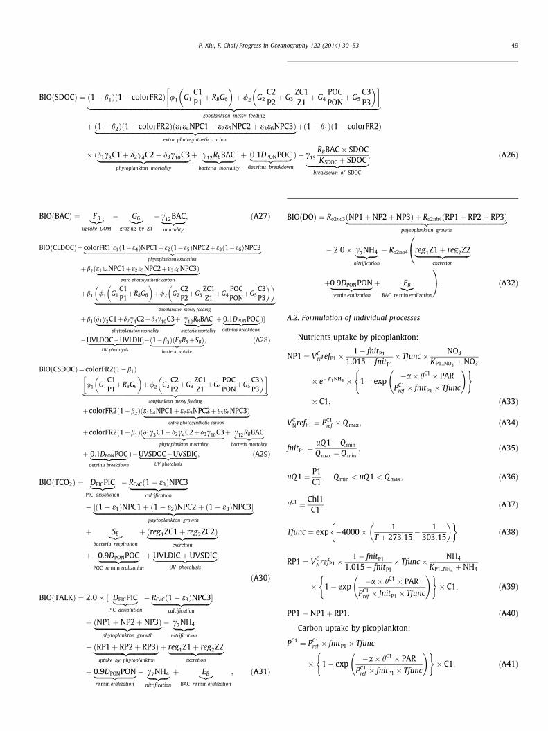
BIOðSDOCÞ ¼ ð1� b1Þð1� colorFR2Þ /1 G1C1P1þ RBG6

� �þ /2 G2

C2P2þ G3

ZC1Z1þ G4

POCPON

þ G5C3P3

� � |fflfflfflfflfflfflfflfflfflfflfflfflfflfflfflfflfflfflfflfflfflfflfflfflfflfflfflfflfflfflfflfflfflfflfflfflfflfflfflfflfflfflfflfflfflfflfflfflfflfflfflfflfflfflfflfflfflfflfflfflfflfflfflfflfflfflfflfflfflfflfflfflfflfflfflfflfflfflfflfflfflfflfflfflfflfflfflffl{zfflfflfflfflfflfflfflfflfflfflfflfflfflfflfflfflfflfflfflfflfflfflfflfflfflfflfflfflfflfflfflfflfflfflfflfflfflfflfflfflfflfflfflfflfflfflfflfflfflfflfflfflfflfflfflfflfflfflfflfflfflfflfflfflfflfflfflfflfflfflfflfflfflfflfflfflfflfflfflfflfflfflfflfflfflfflfflffl}


þ ð1� b2Þð1� colorFR2Þðe1e4NPC1þ e2e5NPC2þ e3e6NPC3Þ|fflfflfflfflfflfflfflfflfflfflfflfflfflfflfflfflfflfflfflfflfflfflfflfflfflfflfflfflfflfflfflfflfflfflfflfflfflfflfflfflfflfflfflfflfflfflfflfflfflfflfflfflfflfflfflfflfflfflffl{zfflfflfflfflfflfflfflfflfflfflfflfflfflfflfflfflfflfflfflfflfflfflfflfflfflfflfflfflfflfflfflfflfflfflfflfflfflfflfflfflfflfflfflfflfflfflfflfflfflfflfflfflfflfflfflfflfflfflffl}extra photosynthetic carbon

þð1� b1Þð1� colorFR2Þ

� ðd1c3C1þ d2c4C2þ d3c10C3|fflfflfflfflfflfflfflfflfflfflfflfflfflfflfflfflfflfflfflfflfflfflfflfflffl{zfflfflfflfflfflfflfflfflfflfflfflfflfflfflfflfflfflfflfflfflfflfflfflfflffl}phytoplankton mortality


þ 0:1DPONPOC|fflfflfflfflfflfflfflfflffl{zfflfflfflfflfflfflfflfflffl}det ritus breakdown

Þ � c13RBBAC� SDOCKSDOC þ SDOC|fflfflfflfflfflfflfflfflfflfflfflfflfflfflfflffl{zfflfflfflfflfflfflfflfflfflfflfflfflfflfflfflffl}

breakdown of SDOC

; ðA26Þ


BIOðBACÞ ¼ FB|{z}uptake DOM


� c12BAC|fflfflfflffl{zfflfflfflffl}mortality

; ðA27Þ

BIOðCLDOCÞ¼ colorFR1½e1ð1�e4ÞNPC1þe2ð1�e5ÞNPC2þe3ð1�e6ÞNPC3|fflfflfflfflfflfflfflfflfflfflfflfflfflfflfflfflfflfflfflfflfflfflfflfflfflfflfflfflfflfflfflfflfflfflfflfflfflfflfflfflfflfflfflfflfflfflfflfflfflfflfflfflfflfflfflfflfflfflffl{zfflfflfflfflfflfflfflfflfflfflfflfflfflfflfflfflfflfflfflfflfflfflfflfflfflfflfflfflfflfflfflfflfflfflfflfflfflfflfflfflfflfflfflfflfflfflfflfflfflfflfflfflfflfflfflfflfflfflffl}phytoplankton exudation

þb2ðe1e4NPC1þe2e5NPC2þe3e6NPC3Þ|fflfflfflfflfflfflfflfflfflfflfflfflfflfflfflfflfflfflfflfflfflfflfflfflfflfflfflfflfflfflfflfflffl{zfflfflfflfflfflfflfflfflfflfflfflfflfflfflfflfflfflfflfflfflfflfflfflfflfflfflfflfflfflfflfflfflffl}extra photosynthetic carbon

þb1 /1 G1C1P1þRBG6

� �þ/2 G2

C2P2þG3

ZC1Z1þG4

POCPON

þG5C3P3

� �� |fflfflfflfflfflfflfflfflfflfflfflfflfflfflfflfflfflfflfflfflfflfflfflfflfflfflfflfflfflfflfflfflfflfflfflfflfflfflfflfflfflfflfflfflfflfflfflfflfflfflfflfflfflfflfflfflfflfflfflfflffl{zfflfflfflfflfflfflfflfflfflfflfflfflfflfflfflfflfflfflfflfflfflfflfflfflfflfflfflfflfflfflfflfflfflfflfflfflfflfflfflfflfflfflfflfflfflfflfflfflfflfflfflfflfflfflfflfflfflfflfflfflffl}


þb1ðd1c3C1þd2c4C2þd3c10C3|fflfflfflfflfflfflfflfflfflfflfflfflfflfflfflfflfflfflfflfflfflfflfflffl{zfflfflfflfflfflfflfflfflfflfflfflfflfflfflfflfflfflfflfflfflfflfflfflffl}phytoplankton mortality


þ 0:1DPONPOC|fflfflfflfflfflfflfflfflffl{zfflfflfflfflfflfflfflfflffl}detritus breakdown

Þ�

�UVLDOC�UVLDIC|fflfflfflfflfflfflfflfflfflfflfflfflfflfflfflffl{zfflfflfflfflfflfflfflfflfflfflfflfflfflfflfflffl}UV photolysis

�ð1�b3ÞðFBRBþSBÞ|fflfflfflfflfflfflfflfflfflfflfflfflfflfflfflffl{zfflfflfflfflfflfflfflfflfflfflfflfflfflfflfflffl}bacteria uptake

; ðA28Þ

BIOðCSDOCÞ¼ colorFR2ð1�b1Þ

/1 G1C1P1þRBG6

� �þ/2 G2

C2P2þG3

ZC1Z1þG4

POCPON

þG5C3P3

� � |fflfflfflfflfflfflfflfflfflfflfflfflfflfflfflfflfflfflfflfflfflfflfflfflfflfflfflfflfflfflfflfflfflfflfflfflfflfflfflfflfflfflfflfflfflfflfflfflfflfflfflfflfflfflfflfflfflfflfflfflffl{zfflfflfflfflfflfflfflfflfflfflfflfflfflfflfflfflfflfflfflfflfflfflfflfflfflfflfflfflfflfflfflfflfflfflfflfflfflfflfflfflfflfflfflfflfflfflfflfflfflfflfflfflfflfflfflfflfflfflfflfflffl}


þcolorFR2ð1�b2Þðe1e4NPC1þe2e5NPC2þe3e6NPC3Þ|fflfflfflfflfflfflfflfflfflfflfflfflfflfflfflfflfflfflfflfflfflfflfflfflfflfflfflfflfflfflfflfflffl{zfflfflfflfflfflfflfflfflfflfflfflfflfflfflfflfflfflfflfflfflfflfflfflfflfflfflfflfflfflfflfflfflffl}extra photosynthetic carbon

þcolorFR2ð1�b1Þðd1c3C1þd2c4C2þd3c10C3|fflfflfflfflfflfflfflfflfflfflfflfflfflfflfflfflfflfflfflfflfflfflfflffl{zfflfflfflfflfflfflfflfflfflfflfflfflfflfflfflfflfflfflfflfflfflfflfflffl}phytoplankton mortality


þ 0:1DPONPOC|fflfflfflfflfflfflfflfflffl{zfflfflfflfflfflfflfflfflffl}detritus breakdown

Þ�UVSDOC�UVSDIC|fflfflfflfflfflfflfflfflfflfflfflfflfflfflfflfflffl{zfflfflfflfflfflfflfflfflfflfflfflfflfflfflfflfflffl}UV photolysis

; ðA29Þ

BIOðTCO2Þ ¼ DPICPIC|fflfflfflffl{zfflfflfflffl}PIC dissolution

� RCaCð1� e3ÞNPC3|fflfflfflfflfflfflfflfflfflfflfflfflfflfflffl{zfflfflfflfflfflfflfflfflfflfflfflfflfflfflffl}calcification

� ½ð1� e1ÞNPC1þ ð1� e2ÞNPC2þ ð1� e3ÞNPC3�|fflfflfflfflfflfflfflfflfflfflfflfflfflfflfflfflfflfflfflfflfflfflfflfflfflfflfflfflfflfflfflfflfflfflfflfflfflfflfflfflfflfflfflfflfflffl{zfflfflfflfflfflfflfflfflfflfflfflfflfflfflfflfflfflfflfflfflfflfflfflfflfflfflfflfflfflfflfflfflfflfflfflfflfflfflfflfflfflfflfflfflfflffl}phytoplankton growth

þ SB|{z}bacteria respiration

þ ðreg1ZC1þ reg2ZC2Þ|fflfflfflfflfflfflfflfflfflfflfflfflfflfflfflfflfflffl{zfflfflfflfflfflfflfflfflfflfflfflfflfflfflfflfflfflffl}excretion

þ 0:9DPONPOC|fflfflfflfflfflfflfflfflffl{zfflfflfflfflfflfflfflfflffl}POC re min eralization

þ UVLDICþ UVSDIC|fflfflfflfflfflfflfflfflfflfflfflfflfflfflfflffl{zfflfflfflfflfflfflfflfflfflfflfflfflfflfflfflffl}UV photolysis

;

ðA30Þ

BIOðTALKÞ ¼ 2:0� ½ DPICPIC|fflfflfflffl{zfflfflfflffl}PIC dissolution

� RCaCð1� e3ÞNPC3|fflfflfflfflfflfflfflfflfflfflfflfflfflfflffl{zfflfflfflfflfflfflfflfflfflfflfflfflfflfflffl}calcification

�

þ ðNP1þ NP2þ NP3Þ|fflfflfflfflfflfflfflfflfflfflfflfflfflfflfflfflffl{zfflfflfflfflfflfflfflfflfflfflfflfflfflfflfflfflffl}phytoplankton growth


� ðRP1þ RP2þ RP3Þ|fflfflfflfflfflfflfflfflfflfflfflfflfflfflfflfflffl{zfflfflfflfflfflfflfflfflfflfflfflfflfflfflfflfflffl}uptake by phytoplankton

þ reg1Z1þ reg2Z2|fflfflfflfflfflfflfflfflfflfflfflfflfflffl{zfflfflfflfflfflfflfflfflfflfflfflfflfflffl}excretion

þ 0:9DPONPON|fflfflfflfflfflfflfflfflffl{zfflfflfflfflfflfflfflfflffl}re min eralization



; ðA31Þ

BIOðDOÞ ¼ Ro2no3ðNP1þ NP2þ NP3Þ þ Ro2nh4ðRP1þ RP2þ RP3Þ|fflfflfflfflfflfflfflfflfflfflfflfflfflfflfflfflfflfflfflfflfflfflfflfflfflfflfflfflfflfflfflfflfflfflfflfflfflfflfflfflfflfflfflfflfflfflffl{zfflfflfflfflfflfflfflfflfflfflfflfflfflfflfflfflfflfflfflfflfflfflfflfflfflfflfflfflfflfflfflfflfflfflfflfflfflfflfflfflfflfflfflfflfflfflffl}phytoplankton growth

� 2:0� c7NH4|fflfflffl{zfflfflffl}nitrification

� Ro2nh4 reg1Z1þ reg2Z2|fflfflfflfflfflfflfflfflfflfflfflfflfflffl{zfflfflfflfflfflfflfflfflfflfflfflfflfflffl}excretion

0@

þ0:9DPONPON|fflfflfflfflfflfflfflfflffl{zfflfflfflfflfflfflfflfflffl}re min eralization


1A: ðA32Þ

A.2. Formulation of individual processes

Nutrients uptake by picoplankton:

NP1 ¼ VCNrefP1 �

1� fnitP1

1:015� fnitP1� Tfunc � NO3

KP1 NO3 þ NO3

� e�W1NH4 � 1� exp�a� hC1 � PAR

PC1ref � fnitP1 � Tfunc

!( )

� C1; ðA33Þ

VCNrefP1 ¼ PC1

ref � Q max; ðA34Þ

fnitP1 ¼uQ1� Q min

Qmax � Q min; ðA35Þ

uQ1 ¼ P1C1

; Q min < uQ1 < Qmax; ðA36Þ

hC1 ¼ Chl1C1

; ðA37Þ

Tfunc ¼ exp �4000� 1T þ 273:15

� 1303:15

� �� ; ðA38Þ

RP1 ¼ VCNrefP1 �

1� fnitP1

1:015� fnitP1� Tfunc � NH4

KP1 NH4 þ NH4

� 1� exp�a� hC1 � PAR


!( )� C1; ðA39Þ

PP1 ¼ NP1þ RP1: ðA40Þ

Carbon uptake by picoplankton:

PC1 ¼ PC1ref � fnitP1 � Tfunc



!( )� C1; ðA41Þ


nP1 ¼ nNO3 �maxNP1PP1

;0:5� �

; ðA42Þ

NPC1 ¼ PC1 � nP1 � PP1: ðA43Þ

Chlorophyll uptake by picoplankton:

qChl1 ¼hN

max � PC1ref � fnitP1

a� hC1 � PAR: ðA44Þ

Nutrients uptake by diatoms:

NP2 ¼ VCNrefP2 �

1� fnitP2

1:015� fnitP2� Tfunc � UNO3S2



!( )� C2; ðA45Þ

VCNrefP2 ¼ PC2


UNO3S2 ¼minNO3

KP2 NO3 þ NO3;

SiO4

KP2 SiO4 þ SiO4

� �� e�W2NH4 ; ðA47Þ


Q max � Q min; ðA48Þ

uQ2 ¼ P2C2

; Q min < uQ2 < Qmax ðA49Þ

hC2 ¼ Chl2C2

; ðA50Þ

RP2 ¼ VCNrefP2 �

1� fnitP2

1:015� fnitP2� Tfunc � UNH4S2



!( )� C2; ðA51Þ

UNH4S2 ¼minNO3

KP2 NO3 þ NO3;

SiO4

KP2 SiO4 þ SiO4

� �� ð1

� e�W2NH4 Þ; ðA52Þ

PP2 ¼ NP2þ RP2; ðA53Þ

Si2N ¼ SiO4=ðKP2 SiO4 þ SiO4ÞNO3=ðKP2 NO3 þ NO3Þ

; 1:0 6 Si2N 6 4:0; ðA54Þ

USiO4 ¼ VCNrefP2 �

1� fnitP2

1:015� fnitP2� Tfunc � SiO4

KP2 SiO4 þ SiO4



!( )� C2

� Si2N: ðA55Þ

Carbon uptake by diatoms:




!( )� C2; ðA56Þ


;0:5� �

; ðA57Þ


Chlorophyll uptake by diatoms:

qChl2 ¼hN



Nutrients uptake by coccolithophorids:

NP3 ¼ VCNrefP3 �

1� fnitP3

1:015� fnitP3� Tfunc � NO3

KP3 NO3 þ NO3

� e�W3NH4 � 1� exp�a� hC3 � PAR


!( )� C3; ðA60Þ

VCNrefP3 ¼ PC3



Q max � Qmin; ðA62Þ

uQ3 ¼ P3C3

; Q min < uQ3 < Q max; ðA63Þ

hC3 ¼ Chl3C3

; ðA64Þ

RP3 ¼ VCNrefP3 �

1� fnitP3

1:015� fnitP3� Tfunc � NH4

KP3 NH4 þ NH4



!( )� C3; ðA65Þ

PP3 ¼ NP3þ RP3: ðA66Þ

Carbon uptake by coccolithophorids:




!( )� C3; ðA67Þ


;0:5� �

; ðA68Þ


Chlorophyll uptake by coccolithophorids:

qChl3 ¼hN



Grazing on picoplankton and bacteria by microzooplankton:

G1 ¼ G1maxf5P1

K1gr þ f5P1þ f6BACZ1; ðA71Þ

G6 ¼ G1maxf6BAC

K1gr þ f5P1þ f6BACZ1; ðA72Þ

f5 ¼q5P1

q5P1þ q6BAC; ðA73Þ

f6 ¼q6BAC

q5P1þ q6BAC: ðA74Þ

Grazing on diatoms, microzooplankton, detritus and coccolitho-phorids by mesozooplankton:

G2 ¼ G2maxf1P2

K2gr þ f1P2þ f2Z1þ f3PONþ f4P3Z2; ðA75Þ


G3 ¼ G2maxf2Z1


G4 ¼ G2maxf3PON


G5 ¼ G2maxf4P3


f1 ¼q1P2

q1P2þ q2Z1þ q3PONþ q4P3; ðA79Þ

f2 ¼q2Z1


f3 ¼q3PON


f4 ¼q4P3

q1P2þ q2Z1þ q3PONþ q4P3: ðA82Þ

Bacteria uptake of LDOM (Anderson and Williams, 1998):

UC ¼ lBmax � RBLDOC

KL þ LDOCBAC; ðA83Þ

UN ¼ UCLDONLDOC

: ðA84Þ

Bacteria uptake of ammonia, DOM, respiration, and ammoniaremineralization:

U�B ¼ lBmax � BACNH4

KB þ NH4: ðA85Þ

(1) If ammonium uptake is sufficient to permit utilization ofDOM, that is, U�B P �UC

UNUC� ð1�r bÞ

RB

� �, then bacteria uptake

of DOM has the form of

FB ¼ ð1� r bÞUC

RB; ðA86Þ

bacteria respiration,

SB ¼ r b� UC; ðA87Þ

remineralization by bacteria,

EB ¼ UCUN

UC� ð1� r bÞ

RB

� �: ðA88Þ

If EB > 0, then UB = 0; otherwise, UB = �EB.
(2) If there is insufficient ammonium, that is,
U�B < �UCUNUC� ð1�r bÞ

RB

� �, then bacteria uptake of ammonia is

obtained by,

UB ¼ U�B; ðA89Þ

bacteria uptake of DOM,

FB ¼ UN þ UB; ðA90Þ

bacteria respiration,

SB ¼ RBFBr b

1� r b; ðA91Þ

remineralization by bacteria,

EB ¼ �UB: ðA92Þ

CDOM photolysis (Bissett et al., 1999a):

UVLDOC ¼ aCLDOCð410Þ � RtUVLDOC� PARð0Þ410

� �

� expZ 0

zKdð300Þdz

; ðA93Þ

UVSDOC ¼ aCSDOCð410Þ � RtUVSDOC� PARð0Þ410

� �

� expZ 0

zKdð300Þdz

; ðA94Þ

UVLDIC ¼ aCLDOCð410Þ � RtUVLDIC� PARð0Þ410

� �

� expZ 0

zKdð300Þdz

; ðA95Þ

UVSDIC ¼ aCSDOCð410Þ � RtUVSDIC� PARð0Þ410

� �

� expZ 0

zKdð300Þdz

; ðA96Þ

aCLDOCð410Þ ¼ a�cdoc � CLDOC; ðA97Þ

aCSDOCð410Þ ¼ a�cdoc � CSDOC; ðA98Þ

Kdð300Þ ¼ ½aCLDOCð410Þ þ aCSDOCð410Þ� � exp½0:0145

� ð410� 300Þ� þ 0:154: ðA99Þ

The dissolution rate for biogenic silica (Jiang et al., 2003):

DSi ¼ ð0:19T=25þ 0:01Þ � expð0:069ðT � 25ÞÞ: ðA100Þ

The air–sea flux of CO2 is calculated using the transfer velocity-wind speed relationships from Wanninkhof (1992):

air � sea CO2 flux ¼ 0:31U2ð660=ScÞ0:5SfðpCO2Þsea � ðpCO2Þairg;ðA101Þ

where U is the wind speed at sea surface and Sc is the Schmidt num-ber for CO2 that can be calculated as:

Sc ¼ 2073:1� 125:62T þ 3:6276T2 � 0:043219T3; ðA102Þ

S is the solubility of CO2 and (pCO2)air is the partial pressure of CO2 inthe air. In the model, we set a spatially uniform distribution of (pCO2)air

observed at the Mauna Loa Observatory (Keeling et al., 1976).Dissolved oxygen (DO) is modeled using constant oxygen-to-ni-

trate and oxygen-to-ammonium ratios. At the surface, air-sea ex-change of O2 is calculated as:

O2 flux ¼ 0:31U2ð660=So2Þ0:5ðDOsat � DOÞ; ðA103Þ

where DOsat is the saturation concentration of DO calculated fromtemperature and salinity. So2 is the Schmidt number for O2 thatcan be calculated as follows:

So2 ¼ 1638:0� 81:83T þ 1:483T2 � 0:008004T3: ðA104Þ

References

Anderson, T.R., Williams, P.J.B., 1998. Modelling the seasonal cycle of dissolvedorganic carbon at station E1 in the English Channel. Estuarine, Coastal and ShelfScience 46, 93–109.

http://refhub.elsevier.com/S0079-6611(13)00227-9/h0035




Anderson, T.R., Pondaven, P., 2003. Non-redfield carbon and nitrogen cycling in theSargasso Sea: pelagic imbalances and export flux. Deep Sea Research 50, 573–591.

Aumont, O., Maier-Reimer, E., Blain, S., Monfray, P., 2003. An ecosystem model ofthe global ocean including Fe, Si, P co-limitation. Global Biogeochem. Cycles 17(2), 1060. http://dx.doi.org/10.1029/2001GB001745.

Babin, M., Stramski, D., Ferrari, G.M., Claustre, H., Bricaud, A., Obolensky, G.,Hoepffner, N., 2003a. Variations in the light absorption coefficients ofphytoplankton, non-algal particles, and dissolved organic matter in coastalwaters around Europe. Journal of Geophysical Research. http://dx.doi.org/10.1029/2001JC000882.

Babin, M., Morel, A., Fournier-Sicre, V., Fell, F., Stramski, D., 2003b. Light scatteringproperties of marine particles in coastal and open ocean waters as related to theparticle mass concentration. Limnology and Oceanography 48 (2), 843–859.

Balch, W.M., Kilpatrick, K.A., Holligan, P., Harbour, D., Fernandez, E., 1996. The 1991coccolithophore bloom in the central North Atlantic. 2. Relating optics tococcolith concentration. Limnology and Oceanography 41 (8), 1684–1696.

Behrenfeld, M.J., Falkowski, P.G., 1997. Photosynthetic rates derived from satellite-based chlorophyll concentration. Limnology and Oceanography 42, 1–20.

Behrenfeld, M.J., Boss, E., Siegel, D.A., Shea, D.M., 2005. Carbon-based oceanproductivity and phytoplankton physiology from space. Global BiogeochemicalCycles 19, GB1006. http://dx.doi.org/10.1029/2004GB002299.

Bissett, W.P., Carder, K.L., Walsh, J.J., Dieterle, D.A., 1999a. Carbon cycling in theupper waters of the Sargasso Sea: II. Numerical simulation of apparent andinherent optical properties. Deep Sea Research: I 46, 271–317.

Bissett, W.P., Walsh, J.J., Dieterle, D.A., Carder, K.L., 1999b. Carbon cycling in theupper waters of the Sargasso Sea: I. Numerical simulation of differential carbonand nitrogen fluxes. Deep Sea Research I 46, 205–269.

Bissett, W.P., Schofield, O., Glenn, S., Cullen, J.J., Miller, W.L., Plueddemann, A.J.,Mobley, C.D., 2001. Resolving the impacts and feedback of ocean optics onupper ocean ecology. Oceanography 14 (3), 30–53.

Bissett, W.P., DeBra, S., Dye, D., 2004. Ecological Simulation (EcoSim) 2.0 TechnicalDescription. FERI Tech. Doc. Num. FERI-2004-0002-U-D, August 10, 2004.Tampa, Fl, 27 pp.

Boss, E., Stramski, D., Bergmann, T., Pegau, W.S., Lewis, M., 2004. Why should wemeasure the optical backscattering coefficient? Oceanography 17 (2), 44–49.

Bricaud, A., Morel, A., Prieur, L., 1983. Optical efficiency factors of somephytoplankters. Limnology and Oceanography 28, 816–832.

Carder, K.L., Steward, R.G., Harvey, G.R., Ortner, P.B., 1989. Marine humic and fulvicacids: their effects on remote sensing of ocean chlorophyll. Limnology andOceanography 34 (1), 68–81.

Chai, F., Dugdale, R.C., Peng, T.-H., Wilkerson, F.P., Barber, R.T., 2002. Onedimensional ecosystem model of the Equatorial Pacific upwelling system. PartI: Model development and silicon and nitrogen cycle. Deep Sea Research: II 49,2713–2745.

Christian, J.R., Anderson, T.R., 2002. Modeling DOM biogeochemistry. In: Hansell,D.A., Carlson, C.A. (Eds.), Biogeochemistry of Marine Dissolved Organic Matter.Academic Press, pp. 717–756.

Coale, K.H., Johnson, K.S., Fitzwater, S.E., Gordon, R.M., Tanner, S., Chavez, F.P.,Ferioli, L., Sakamoto, C., Rogers, P., Millero, F., Steinberg, P., Nightingale, P.,Cooper, D., Cochlan, W.P., Landry, M.R., Constantinou, J., Rollwagen, G., Trasvina,A., Kudela, R., 1996. A massive phytoplankton bloom induced by an ecosystem-scale iron fertilization experiment in the equatorial Pacific Ocean. Nature 383,495–501.

Dore, J.E., Letelier, R.M., Church, M.J., Lukas, R., Karl, D.M., 2008. Summerphytoplankton blooms in the oligotrophic North Pacific Subtropical Gyre:historical perspective and recent observations. Progress in Oceanography 76, 2–38.

DuRand, M.D., Olson, R.J., Chisholm, S.W., 2001. Phytoplankton populationdynamics at the Bermuda Atlantic Time-series station in the Sargasso Sea.Deep Sea Research: II 48, 1983–2003.

Eppley, R.W., Chavez, F.P., Barber, R.T., 1992. Standing stocks of particulate carbonand nitrogen in the Equatorial Pacific at 150�W. Journal of Geophysical Research97, 655–661.

Fennel, K., Abbott, M.R., Spitz, Y.H., Richman, J.G., Nelson, D.M., 2003. Modelingcontrols of phytoplankton production in the southwest Pacific sector of theSouthern Ocean. Deep-Sea Research II 50, 769–798.

Fujii, M., Boss, E., Chai, F., 2007. The value of adding optics to ecosystem models: acase study. Biogeosciences 4, 817–835.

Fujii, M., Chai, F., 2007. Modeling carbon and silicon cycling in the equatorial Pacific.Deep Sea Research II 54, 496–520.

Garcia, H.E., Locarnini, R.A., Boyer, T.P., Antonov, J.I., 2006. World Ocean Atlas 2005.In: Levitus, S. (Ed.), Nutrients Phosphate Nitrate Silicate. Atlas NESDIS 64, vol. 4.U.S. Government Printing Office, Washington, DC.

Geider, R.J., Macintyre, H.L., Kana, T.M., 1998. A dynamic regulatory model ofphytoplanktonic acclimation to light, nutrients, and temperature. Limnologyand Oceanography 43, 679–694.

Goebel, N.L., Edwards, C.A., Zehr, J.P., Follows, M.J., 2010. An emergent communityecosystem model applied to the California Current System. Journal of MarineSystem 83, 221–241.

Gordon, H.R., Boynton, G.C., Balch, W.M., Groom, S.B., Harbour, D.S., Smyth, T.J.,2001. Retrieval of coccolithophore calcite concentration from SeaWiFS imagery.Geophysical Research Letters 28, 1587–1590.

IOCCG, 2000. Remote sensing of ocean color in coastal, and other optically complexwaters. In: Sathyendranath, S. (Ed.), Reports of the International Ocean-ColourCoordinating Group, No. 3, Dartmouth, Canada.

IOCCG, 2006. Remote sensing of inherent optical properties: fundamentals, test ofalgorithms, and applications. In: Lee, Z.-P. (Ed.), Reports of the InternationalOcean-Colour Coordinating Group, No. 5, Dartmouth, Canada.

Jiang, M.-S., Chai, F., Barber, R.T., Dugdale, R.C., Wilkerson, F., Peng, T.-H., 2003. Anitrate and silicate budget in the Equatorial Pacific Ocean: a coupled biological-physical model study. Deep Sea Research: II 50, 2971–2996.

Kalnay, E., Kanamitsu, M., Kistler, R., Collins, W., Deaven, D., Gandin, L., Iredell, M.,Saha, S., White, G., Woollen, J., Zhu, Y., Chelliah, M., Ebisuzaki, W., Higgins, W.,Janowiak, J., Mo, K.C., Ropelewski, C., Wang, J., Jenne, R., Joseph, D., 1996. TheNCEP/NCAR 40-year reanalysis project. Bulletin of the American MeteorologicalSociety 77, 437–471.

Keeling, C.D., Bacastow, R.B., Bainbridge, A.E., Ekdahl, C.A., Guenther, P.R.,Waterman, L.S., 1976. Atmospheric carbon dioxide variations at Mauna LoaObservatory, Hawaii. Tellus 28, 538–551.

Key, R.M., Kozyr, A., Sabine, C.L., Lee, K., Wanninkhof, R., Bullister, J., Feely, R.A.,Millero, F., Mordy, C., Peng, T.-H., 2004. A global ocean carbon climatology:results from GLODAP. Global Biogeochemical Cycles 18, GB4031.

Kishi, M.J., Kashiwai, M., Ware, D.M., Megrey, B.A., Eslinger, D.L., Werner, F.E.,Noguchi-Aita, M., Azumaya, T., Fujii, M., Hashimoto, S., Huang, D., Iizumi, H.,Ishida, Y., Kang, S., Kantakov, G.A., Kim, H., Komatsu, K., Navrotsky, V.V., Smith,S.L., Tadokoro, K., Tsuda, A., Yamamura, O., Yamanaka, Y., Yokouchi, K., Yoshie,N., Zhang, J., Zuenko, Y.I., Zvalinsky, V.I., 2007. NEMURO—a lower trophic levelmodel for the North Pacific marine ecosystem. Ecological Modellling 202, 12–25.

Large, W.G., Pond, S., 1982. Sensible and latent heat flux measurements over theocean. Journal of Physical Oceanography 12, 464–482.

Lee, Z.P., Carder, K.L., Arnone, R.A., 2002. Deriving inherent optical properties fromwater color: a multi-band quasi-analytical algorithm for optically deep waters.Applied Optics 41, 5755–5772.

Lee, Z., Du, K., Arnone, R., Liew, S., Penta, B., 2005. Penetration of solar radiation inthe upper ocean: a numerical model for oceanic and coastal waters. Journal ofGeophysical Research 110, C09019. http://dx.doi.org/10.1029/2004JC002780.

Levy, M., Memery, L., Andre, J.-M., 1998. Simulation of primary production andexport fluxes in the Northwestern Mediterranean Sea. Journal of MarineResearch 56, 197–238.

Locarnini, R.A., Mishonov, A.V., Antonov, J.I., Boyer, T.P., Garcia, H.E., 2006. WorldOcean Atlas 2005. In: Levitus, S. (Ed.), Temperature, NOAA Atlas NESDIS 61, vol.1. U.S. Government Printing Office, Washington, DC.

Martin, J.H., Coale, K.H., Johnson, K.S., Fitzwater, S.E., Gordon, R.M., Tanner, S.J.,Hunter, C.N., Elrod, V.A., Nowicki, J.L., Coley, T.L., Barber, R.T., Lindley, S.,Watson, A.J., van Scoy, K., Law, C.S., Liddicoat, M.I., Ling, R., Stanton, T., Stockel, J.,Collins, C., Anderson, A., Bidigare, R., Ondrusek, M., Latasa, M., Millero, F.J., Lee,K., Yao, W., Zhang, J.Z., Friederich, G., Sakamoto, C., Chavez, F., Buck, K., Kolber,Z., Greene, R., Falkowski, P., Chisholm, S.W., Hoge, F., Swift, R., Yungel, J., Turner,S., Nightingale, P., Hatton, A., Liss, P., Tindale, N.W., 1994. Testing the ironhypothesis in ecosystems of the equatorial Pacific Ocean. Nature 371, 123–129.

Millan-Nuñez, R., Alvarez-Borrego, S., Trees, C.C., 1996. Relationship between deepchlorophyll maximum and surface chlorophyll concentration in the CaliforniaCurrent System. CalCOFI Report, 37.

Moore, J.K., Doney, S.C., Kleypas, J.A., Glover, D.M., Fung, I.Y., 2002. An intermediatecomplexity marine ecosystem model for the global domain. Deep Sea Research:II 49, 403–462.

Morel, A., 1974. Optical properties of pure water and pure seawater. In: Jerlov, E.,Steeman Nielsen (Eds.), Optical Aspects of Oceanography. Academic Press, NewYork, pp. 1–24.

Nanninga, H.J., Tyrrell, T., 1996. Importance of light for the formation of algalblooms by Emiliania huxleyi. Marine Ecology Progress Series 136, 195–203.

Nelson, N.B., Siegel, D.A., 2013. The global distribution and dynamics ofchromophoric dissolved organic matter. Annual Review of Marine Science 5,447–476.

Pope, R.M., Fry, E.S., 1997. Absorption spectrum (380–700 nm) of pure water. II.Integrating cavity measurements. Applied Optics 36, 8710–8723.

Ragueneau, O., Treguer, P., Leynaert, A., Anderson, R.F., Brzezinski, M.A., Demaster,D.J., Dugdale, R.C., Dymond, J., Fischer, G., Francois, R., Heinze, C., Maier-Reimer,E., Martin-Jezequel, V., Nelson, N.B., Queguiner, B., 2000. A review of the Si cyclein the modern ocean: recent progress and missing gaps in the application ofbiogenic opal as a paleoproductivity proxy. Global and Planetary Change 26,317–365.

Rothstein, L.M., Cullen, J.J., Abbott, M., Chassignet, E.P., Denman, K., Doney, S.C.,Ducklow, H., Fennel, K., Follows, M., Haidvogel, D., Hoffman, E., Karl, D.M.,Kindle, J., Lima, I., Maltrud, M., McClain, C., McGillicuddy, D., Olascoaga, M.J.,Spitz, Y., Wiggert, J., Yoder, J., 2006. Modeling ocean ecosystems: the PARADIGMprogram. Oceanography 19 (1), 22–51.

Shchepetkin, A.F., McWilliams, J.C., 2005. The regional ocean modeling system: asplit-explicit, free-surface, topography following coordinates ocean model.Ocean Modelling 9, 347–404.

Shulman, I., Frolov, S., Anderson, S., Penta, B., Gould, R., Sakalaukus, P., Ladner, S.,2013. Impact of bio-optical data assimilation on short-term coupled physical,bio-optical model predictions. Journal of Geophysical Research Oceans 118.http://dx.doi.org/10.1002/jgrc.20177.

Siegel, D.A., Maritorena, S., Nelson, N.B., Behrenfeld, M.J., McClain, C.R., 2005.Colored dissolved organic matter and its influence on the satellite-basedcharacterization of the ocean biosphere. Geophysical Research Letters 32,L20605. http://dx.doi.org/10.1029/2005GL024310.

Smith, R.C., Baker, K.S., 1978. The bio-optical state of ocean waters and remotesensing. Limnology and Oceanography 23, 247–259.




http://dx.doi.org/10.1029/2001GB001745

http://dx.doi.org/10.1029/2001JC000882

http://dx.doi.org/10.1029/2001JC000882









http://dx.doi.org/10.1029/2004GB002299





















































































http://dx.doi.org/10.1029/2004JC002780











































http://dx.doi.org/10.1002/jgrc.20177

http://dx.doi.org/10.1029/2005GL024310




Stramski, D., Reynolds, R.A., Kahzu, M., Mitchell, B.G., 1999. Estimation ofparticulate organic carbon in the ocean from satellite remote sensing. Science285 (5433), 239–242.

Strom, S.L., Benner, R., Ziegler, S., Dagg, M.J., 1997. Planktonic grazers are apotentially important source of marine dissolved organic carbon. Limnologyand Oceanography 42, 1364–1374.

Sumata, H., Hashioka, T., Suzuki, T., Yoshie, N., Okunishi, T., Aita, M.N., Sakamoto,T.T., Ishida, A., Okada, N., Yamanaka, Y., 2010. Effect of eddy transport on thenutrient supply into the euphotic zone simulated in an eddy-permitting oceanecosystem model. Journal of Marine System 83, 67–87.

Swan, C.M., Siegel, D.A., Nelson, N.B., Carlson, C.A., Nasir, E., 2009. Biogeochemicaland hydrographic controls on chromophoric dissolved organic matterdistribution in the Pacific Ocean. Deep Sea Research: I 56, 2175–2192.

Tian, R.C., Vézina, A.F., Legendre, L., Ingram, R.G., Klein, B., Packard, T., Roy, S.,Savenkoff, C., Silverberg, N., Therriault, J.-C., Tremblay, J.-E., 2000. Effects ofpelagic food-web interactions and nutrient remineralization on thebiogeochemical cycling of carbon: a modeling approach. Deep Sea Research: II47, 637–662.

Vallino, J.J., 2000. Improving marine ecosystem models: use of data assimilation andmesocosm experiments. Journal of Marine Research 58, 117–164.

Volkman, J.K., Tanoue, E., 2002. Chemical and biological studies of particulateorganic matter in the ocean. Journal of Oceanography 58, 265–279.

Walsh, J.J., Dieterle, A.D., Muller-Karger, F.E., Bohrer, R., Bissett, W.P., Varela, R.J.,Aparicio, R., Diaz, R., Thunell, R., Taylor, G.T., Scranton, M.I., Fanning, K.A.,Peltzer, E.T., 1999. Simulation of carbon–nitrogen cycling during springupwelling in the Cariaco Basin. Journal of Geophysical Research 104 (C4),7807–7825.

Wanninkhof, R., 1992. Relationship between wind speed and gas exchange over theocean. Journal of Geophysical Research 97, 7373–7382.

Ward, B.B., 2000. Nitrification and the marine nitrogen cycle. In: Kirchman, D.L.(Ed.), Microbial Ecology of the Oceans. Wiley, New York, pp. 427–453.

Werdell, P.J., Bailey, S.W., 2002. The SeaWiFS Bio-optical Archive and StorageSystem (SeaBASS): current architecture and implementation. In: Fargion, G.S.,McClain, C.R. (Eds.), NASA Tech. Memo. 2002-211617, NASA Goddard SpaceFlight Center, Greenbelt, Maryland, 45 pp.

Wetzel, R.G., Hatcher, P.G., Bianchi, T.S., 1995. Natural photolysis by ultravioletirradiance or recalcitrant dissolved organic matter to simple substrates for rapidbacterial metabolism. Limnology and Oceanography 40 (8), 1369–1380.

Xiu, P., Chai, F., 2012. Spatial and temporal variability in phytoplankton carbon,chlorophyll, and nitrogen in the North Pacific. Journal of Geophysical Research117, C11023. http://dx.doi.org/10.1029/2012JC008067.

Yamanaka, Y., Yoshie, N., Fujii, M., Aita, M.N., Kishi, M., 2004. An ecosystem modelcoupled with nitrogen–silicon–carbon cycles applied to Station A7 in thenorthwestern Pacific. Journal of Oceanography 60, 227–241.

Yamashita, Y., Tanoue, E., 2009. Basin scale distribution of chromophoric dissolvedorganic matter in the Pacific Ocean. Limnology and Oceanography 54, 598–609.

Yentsch, C.S., Phinney, D.A., 1989. A bridge between ocean optics and microbialecology. Limnology and Oceanography 34, 1694–1705.

Zepp, R.G., Schlotzhauer, P.F., 1981. Comparison of photochemical behavior ofvarious humic substances in water: III. Spectroscopic properties of humicsubstances. Chemosphere 10 (5), 479–486.



































http://dx.doi.org/10.1029/2012JC008067











connections between physical, optical and biogeochemical...

Documents