connectionism and the dynamical … and the dynamical approach to cognition 237 8.2 basic concepts...
TRANSCRIPT

CONNECTIONISM AND THE DYNAMICAL APPROACH TO COGNITION 235
8
CONNECTIONISM AND THE DYNAMICAL
APPROACH TO COGNITION
8.1 Are We on the Road to a Dynamical Revolution?
We saw in chapter 1 that connectionism has its roots in the 1940s, when ideas aboutthe nervous system, computation, and intelligence came together synergistically. Webriefly traced the path from formal neurons to perceptrons and noted that eventsin the 1960s led to a period in which these neural network models became over-shadowed by symbolic models of intelligence. With the rise of connectionism in the1980s neural networks regained prominence, and for two decades the two approacheshave each sought to dominate cognitive science.
This is part of a larger story. The energetic collaborations of the 1940s hadmultiple, sometimes intertwined strands, of which the best known is an emphasis onfeedback and control in the cybernetics of Norbert Wiener and others. This requiredattention to the dynamics of change in time, an aspect of the functioning of systemswhich has often been ignored by connectionists (though not by Stephen Grossbergand his group, who continued to advance network research during the period whensymbolic models were dominant; see Grossberg, 1982). In an even broader context,the dynamics of complex physical systems have been mathematically describable atleast since Newton (building on work by Galileo) formulated his three laws ofmotion and developed the calculus to gain the ability to predict specific planetaryconfigurations. New geometrical approaches to dynamics by Poincaré in the latenineteenth century prepared the way for the rise of Dynamical Systems Theory(DST) in the twentieth century. Initially applied primarily to physical phenomenasuch as eddies in a stream (Landau, 1944), by the 1980s DST was being extended tomotor coordination by Michael Turvey, Peter Kugler, and J. A. Scott Kelso (seeKelso, 1995) and by the 1990s to the development not only of coordinated activitybut also more cognitive capacities (see the 1994 book by Esther Thelen and LindaSmith). Although the mathematics of nonlinear dynamical systems can be daunting,DST has spawned compelling graphics that help to provide an intuitive grasp of keyconcepts (among the suggested readings at the end of the chapter, see especially thecopiously illustrated introduction by Abraham and Shaw, 1992).
The idea that cognition is dynamic and can best be understood using the tools ofDST attracted increasing attention across the 1990s but is still somewhat of a fron-tier outpost in cognitive science. Much of the excitement was conveyed in Mind asMotion, a 1995 book originating in a 1991 conference which brought together many

236 CONNECTIONISM AND THE DYNAMICAL APPROACH TO COGNITION
of the pioneering modelers. The editors, Robert Port and Timothy van Gelder,wanted to convince a broad audience that DST has revolutionary implications forcognitive science. In an introductory chapter they characterized cognitive science aswedded to what they call the computational approach (i.e., symbolic modeling) andcalled for a change, contending that “dynamical and computational systems arefundamentally different kinds of systems, and hence the dynamical and computa-tional approaches to cognition are fundamentally different in their deepest founda-tions” (van Gelder and Port, 1995, p. 10). Further, they portrayed the emergence ofthe dynamical approach in cognitive science as a Kuhnian revolution:
The computational approach is nothing less than a research paradigm in Kuhn’s classicsense. It defines a range of questions and the form of answers to those questions (i.e.,computational models). It provides an array of exemplars – classic pieces of researchwhich define how cognition is to be thought about and what counts as a successfulmodel. . . . [T]he dynamical approach is more than just powerful tools; like the com-putational approach, it is a worldview. The cognitive system is not a computer, it is adynamical system. It is not the brain, inner and encapsulated; rather, it is the wholesystem comprised of nervous system, body, and environment. The cognitive system isnot a discrete sequential manipulator of static representational structures; rather, it is astructure of mutually and simultaneously influencing change. Its processes do not takeplace in the arbitrary, discrete time of computer steps; rather, they unfold in the realtime of ongoing change. . . . The cognitive system does not interact with other aspectsof the world by passing messages or commands; rather, it continuously coevolves withthem. . . . [T]o see that there is a dynamical approach is to see a new way of conceptu-ally reorganizing cognitive science as it is currently practiced. (van Gelder and Port,1995, pp. 2–4)
If computational and dynamical worldviews are poles apart, connectionism occupiesa somewhat more ambiguous territory in between. Highly interactive networks,such as Boltzmann machines, are dynamical systems of considerable interest inprinciple. In practice, they are hard to use and hard to analyze even with theavailability of DST tools. Feedforward networks have made the greatest inroadsinto cognitive science, in part due to their tractability, but the only aspect of thisarchitecture that is dynamical is the adaptation of weights during learning. Mostconnectionist models, even interactive ones, carry some symbolic/computationalbaggage and therefore are not the best poster children for van Gelder and Port’srevolution. We see a somewhat different future, in which connectionist modelingcan benefit from both computational and dynamical approaches and can sometimeseven combine them within the analysis of a single network.
In what follows we will introduce some basic dynamical concepts and tools insection 8.2; describe how the simplest concepts have been utilized in four areas ofnetwork research in 8.3; and describe how the concept of chaos has been utilized intwo network models in 8.4. Then in 8.5 we return to philosophical issues raised byvan Gelder and Port. From their overall claim that classic connectionism occupiesan untenable halfway position between the computational and dynamical approaches,we move to more specific arguments concerning explanation (countered by Bechtel)and representation (countered by Clark and Wheeler). The counter-arguments leadtowards a more inclusive cognitive science, and in 8.6 we discuss a controversialversion offered by philosophers Terrence Horgan and John Tienson. Let us start,then, by introducing some concepts and tools from the mathematical core of thedynamical approach: dynamical systems theory (DST).

CONNECTIONISM AND THE DYNAMICAL APPROACH TO COGNITION 237
8.2 Basic Concepts of DST: The Geometry of Change
8.2.1 Trajectories in state space: Predators and prey
If a picture is generally worth a thousand words, in the case of dynamical systemstheory each picture is worth at least ten times that many: among DST’s innovationsis the adroit use of geometrical representations to help conceptualize how systemschange. The simplest picture is a plot of the states traversed by a system throughtime, that is, the system’s trajectory through state space. The trajectory is a continu-ous curve if the system is defined in real time, or a sequence of points in discretetime. Each dimension of state space corresponds to one variable of the system, andeach point in the space corresponds to one of the possible states of the system. Forsystems with one continuous variable, the state space is a range of values on onedimension (e.g., the frequency of a tone; the height of a person; the firing rate of aneuron; the population size of a species in its habitat). The trajectory of a pure toneis a regular oscillation between two values (if a time dimension is added to the plot,a sine wave is obtained). A trajectory for height starts with an infant’s height at birthand rises (irregularly) over time.
To move up to a two-dimensional state space, the most obvious way is to consideran additional variable; for example, you can visualize your child’s growth by graphingheight and weight on orthogonal axes and plotting a point each week; connecting thepoints approximates the child’s trajectory through height-weight space in real time.Another way of moving up to a two-dimensional state space is to examine the samevariable for two different individuals (or neurons, populations, network units, etc.).Keep adding more, and you end up with a high-dimensional system. For example,the activation values across a 90-unit output layer in a feedforward connectionistnetwork can be represented as a single point in a 90-dimensional state space – eachunit’s activation is treated as a separate variable of the system. If the network isfeedforward, its response to an input is one point in the space. If it is interactive, thechanging activation values are represented as a sequence of points – that is, as atrajectory through activation state space – but the outcome may be similar sincesome trajectories simply converge on a point and remain there.
A two-dimensional state space is much easier to visualize than a 90-dimensionalone, so we will use the case of two species in a predator–prey relationship to illus-trate some key concepts (the case is described by Ralph Abraham and ChristopherShaw, 1992, pp. 82–5). The classic account was proposed independently by AlfredJames Lotka (1925) and Vita Volterra (1926). Our first picture, figure 8.1(a), showsseveral variations on an idealized cyclic trajectory (also called a periodic trajectory) inthe state space for number of prey (horizontal axis) and number of predators (ver-tical axis); it was inspired by periodicity in the population sizes of different speciesof fish in the Adriatic Sea. To understand the cyclic changes in population size, fourparts of the outermost curve (labeled I–IV) can be considered separately. (See belowfor discussion of the whole family of curves.) When there are relatively few of bothpredators and prey, the number of predators declines for lack of food while thenumber of prey increases for lack of predators (region I). The increase in prey,though, provides a more ample food source for the predators, and beyond a transi-tion point, the number of predators will begin to increase along with the number ofprey (region II). But the increase in predators results in increased consumption of

238 CONNECTIONISM AND THE DYNAMICAL APPROACH TO COGNITION
Num
ber
of p
reda
tors
(c)(b)(a)
IV III
III
Number of prey
prey, so after another transition point the number of prey declines while predatorscontinue to increase (region III). But eventually the shrinking prey population leadsto starvation for predators and both predators and prey decline in population (regionIV). When the number of predators becomes sufficiently low, the number of preywill begin to increase again (region I). And so forth: in principle, each population’ssize is predicted to oscillate (move between two extremes) forever, with the sameperiod (elapsed time) on each cycle. The prediction derives from the Lotka–Volterraequations, in which the rate of change of each population depends on the currentnumber of prey (x) and predators (y) as well as the values of the control parameters(A, B, C, and D):
∂∂x
ty x ( )= −A B (1)
∂∂y
ty ( )= −C Dx (2)
To obtain a cyclic trajectory using these equations, an appropriate set of para-meter values must be identified (not all values will produce such a trajectory).1 Asshown in figure 8.1(a) for one such set of values, the equations then yield a family ofconcentric closed curves around a central equilibrium point. Within that family, theparticular curve – ranging from no oscillation at the center to the extreme populationswings of the largest-diameter circle – depends upon the initial values of x and y.Once the system embarks on one of these trajectories, it will repeat it indefinitely –unless perturbed by some change outside the system. For example, unusually hightemperatures may increase the predators’ mortality rate, D, and also affect repro-duction and predation rates, reflected in A–C.
Another way to get different trajectories is to change the equations. In fact, laterresearchers found that the Lotka–Volterra equations alone are unrealistic (e.g., theymake no provision for competition among prey or predators for limited resources).One kind of revision to the system of equations adds “ecological friction” (by ana-logy to the physical friction that brings a pendulum asymptotically to rest by damp-ing its oscillations). Figure 8.1(b) shows how this produces a very characteristicDST state space plot. The illustrative trajectory now has two parts. The pointattractor at the center (also called the limit point) is stable – if exactly these predatorand prey population sizes are attained, the system is in equilibrium and will remain
Figure 8.1 Possible trajectories through state space for interacting predator and preypopulations: (a) cyclic trajectories (no attractor); (b) point attractor with spiraling transient;(c) cyclic attractor with spiraling transients beginning at points inside and outside of it.

CONNECTIONISM AND THE DYNAMICAL APPROACH TO COGNITION 239
in that state. Thus, the attractor is the stable part of the trajectory, and can be viewedas describing the long-term behavior of the system. The curve that leads to theattractor is a transient, the part of the trajectory that the system traverses as it movesfrom its initial state towards equilibrium. The spiraling transients in this systemreflect a story similar to the one we told for sections I–IV of the outer cycle in figure8.1(a), except that here the system approaches the equilibrium point as the oscilla-tions in population size diminish in amplitude. When the transient spirals towards apoint like this, the system is a damped oscillator and the point attractor is also calleda focal point.
Crucially, trajectories from many different initial states will converge on the samefocal point: for various initial numbers of predators and prey, the populations willapproach this point of equilibrium along an appropriate, spiraling transient. In fact,it is primarily the convergence of nearby trajectories to this equilibrium point thatqualifies it as an attractor (cf. the equilibrium point in figure 8.1(a), which is not anattractor); and it is specifically a point attractor (limit point) because the subset ofstate space to which the trajectories converge (the limit set) consists of just one point.The set of all initial states whose trajectories converge on this attractor is its basin ofattraction (generally a region of state space but possibly the entire space). The statespace – also called phase space – filled with the possible trajectories of this system isits phase portrait. In figure 8.1(b) this was reduced, for display purposes, to a repres-entation of the point attractor (by convention, a small solid circle) and one typicaltrajectory. For systems with multiple attractors (and perhaps other special features,such as repellors, saddle nodes, and the separatrices that may form boundaries be-tween basins), a larger number of trajectories or special display conventions areneeded to convey the essentials of the phase portrait.
This is a good place to pause and note that considerable idealization is involved inusing even the modified system of equations to model changes in the populationsizes of two species in a predator–prey relationship. First, the real-life populationsare not a closed system; as already mentioned, external factors such as ocean tem-perature can affect parameter values. Second, here as in many other dynamicalsystems (those classified as dissipative), convergence is asymptotic – the state of thesystem approaches the attractor as time approaches infinity. Beyond the formalnature of this characterization, it also assumes a continuity that cannot be attained inpopulation dynamics. Each birth or death brings a discrete change in the value of xor y. At best these values will jiggle around in the vicinity of the equilibrium point asindividuals are born and die. This leads to another notion that is worth makingexplicit: even if the system could reach true equilibrium, what is stable is the valueof two collective variables. Out in the Adriatic Sea, individual fish are still givingbirth and dying, eating or being eaten. Trajectories of change in the lives of indi-vidual fish are not inconsistent with lack of change in the size of their two populations.
A phase portrait that is somewhat more realistic for the Adriatic case (though stillidealized) can be obtained by making one more revision to the system of equations.Figure 8.1(c) shows a cyclic attractor (also called a periodic attractor or limit cycle)along with a few of the possible transients. This is a form of stable behavior that atleast involves movement – the state of the system endlessly cycles around in statespace rather than remaining at a single point as in (b). But the comparison to portrait(a) is even more informative. The circle in the middle of (c) looks the same as oneof the circles in (a), but the dynamics producing it are quite different. As a cyclicattractor, it is the stable part of a variety of trajectories rather than a single trajectory.

240 CONNECTIONISM AND THE DYNAMICAL APPROACH TO COGNITION
That is, in (c) many different starting points all converge on the same circle (that iswhy it is called an attractor), whereas in (a) the starting point is already part of thecircle and determines its diameter.2 (Note that although both of these cycles arecircles, in other systems they might be any sort of closed curve; we will see muchodder-shaped limit cycles in figure 8.3(a).) Examining (c) more closely, it can beseen that a trajectory that begins with many predators and many prey and anotherthat begins with very few predators but almost as many prey both have transientsthat converge on the limit cycle; that is, the long-term behavior of both trajectoriesis the same. Trajectories with transients inside the limit cycle also converge on it; inthe one exemplar shown in (c), the trajectory begins near a point repellor (a pointfrom which trajectories diverge – the opposite of an attractor – shown conventionallyas a small hollow circle) and spirals out to converge on the limit cycle. Thus, thebasin of attraction is extensive.
8.2.2 Bifurcation diagrams and chaos
Some systems exhibit behavior that is more complex than in figure 8.1. In additionto the possibility of multiple attractors and other special features, there exist un-stable trajectories which appear random despite following a deterministic path (i.e.,the trajectory never repeats itself, but from any given point in the state space thereis an algorithm that determines the next point). Perhaps more dramatically thannecessary, this is called a chaotic trajectory. When the (infinite number of ) possiblechaotic trajectories of a system exhibit the characteristics of an attractor, the systemis said to have a chaotic attractor. In particular, trajectories that begin near eachother in the (infinitely large) limit set of the attractor will tend to diverge (a charac-teristic known as sensitive dependence on initial conditions), while trajectories thatbegin in the limit set’s basin of attraction will converge on it. Chaotic attractors tendto be topologically complex. One of the simpler examples starts with the doughnut-shaped torus, which can be thought of as offering an infinite number of cyclictrajectories. A system with a torus attractor in its phase portrait will exhibit quasi-periodic behavior (continuously circling the torus but not repeating any particularcycle). However, the behavior becomes unstable for a torus in a very high-dimen-sional space: the system samples various cyclic trajectories along the surface of thetorus, jumping from one to the next at irregular intervals. This unstable sampling ofcycles is a chaotic trajectory. And this glimpse of a complex field of mathematics willhave to suffice here.
Chaotic behavior is one innovative concept of DST; another is the importance ofparameter values in whether a system exhibits that behavior. Even simple nonlinearsystems may exhibit phase transitions (rapid shifts from one phase portrait toanother) when the value of one or more control parameters changes slightly. Forexample, a single difference equation may produce a single point attractor, a cyclicattractor (limit cycle), or a chaotic attractor for x depending on the value of onecontrol parameter A. The rapid transition in dynamics, brought about by a smallbut critical change in the parameter, is referred to mathematically as a bifurcation.The simplest example (from which the general term derives) is a pitchfork bifurca-tion, wherein a single point attractor splits in two. To explain and illustrate thisconcept, we will use a bifurcation diagram to display the varied behavior of a well-studied type of system defined in discrete time. It is specified by the logistic equa-

CONNECTIONISM AND THE DYNAMICAL APPROACH TO COGNITION 241
tion (which should not be confused with the logistic activation function introducedin chapter 2):
xt+1 = Axt (1 − xt) (3)
where x is a variable with range 0<x<1 and A is a control parameter from the range0<A<4. The subscripts t and t + 1 index successive time-steps t0, t1, t2, t3, and soforth; any value xt+1 depends in part on the value xt on the previous time-step. Wecan begin by simply examining the sequence of values taken by x (its trajectory)when A is fixed, as it is generally assumed to be for a given system. Here is thecalculation of the first five points of the trajectory when A = 3 and the initial statex0 = 0.5:
x1 = 3 × 0.5 × 0.5 = 0.75x2 = 3 × 0.75 × 0.25 = 0.5625x3 = 3 × 0.5625 × 0.4375 = 0.7383x4 = 3 × 0.7383 × 0.2617 = 0.5796x5 = 3 × 0.5796 × 0.4204 = 0.7310
It can be seen even from these few points that the system is behaving as a dampedoscillator (its behavior through much but not all of the stated range). It is conver-ging on a point attractor at 0.6667 and the transient is a discrete version of thecontinuous spiral in figure 8.1(b). That is, it alternates between high and low valuesrather than spiraling between them. (In both cases, since the oscillation is damped,the high and low values themselves keep changing as the system converges on theattractor.) If a different initial value of x is used, the high and low values may beginfurther apart or closer together but will converge on the same attractor value of0.6667.
From all this detail about the trajectories of x when A = 3, the only informationneeded for the bifurcation diagram is the value of the point attractor, 0.6667. Ingeneral the bifurcation diagram for the logistic equation shows, for values of Awithin some range, the stable (long-term) values that x may attain. The transientsone would obtain from different initial values of x are ignored; only the stable valueor values to which they converge are plotted. A single stable value is the simplestoutcome, and that is how this equation behaves when A is between 0 and 3.
Figure 8.2 shows the bifurcation diagram for values of A between 2.6 and 4.0.This catches some of the simple part of the range. The first bifurcation (a pitchfork)appears just beyond A = 3 where x’s stable long-term behavior suddenly switches toan alternation between two values (that is, the point attractor is replaced by aperiodic attractor with periodicity of 2). These values (the prongs of the fork) driftfurther apart as A increases, but what matters most is that the dynamics are qualitat-ively different before vs. after the point of transition, which is called a bifurcationpoint. Just beyond 3.4 another bifurcation point is reached, and the system’s period-icity increases to 4.
At a value of A beyond 3.6 a different kind of bifurcation begins to develop, one inwhich the attractor ceases to be periodic and becomes chaotic. The darkened regionis a rough representation of the fact that x is taking a nonrepeating sequence ofvalues. The value at each time step is deterministic since it is generated by equation(3), but each value is a new one. The new phase portrait contains a chaotic attractor,which changes form as the value of A increases. Interestingly, there are even values

242 CONNECTIONISM AND THE DYNAMICAL APPROACH TO COGNITION
Figure 8.2 Bifurcation plot of the logistic function (1) for values of A between 2.6and 4.0. For values of A less than 3.0 the function settles into a point attractor. Above3.0 it bifurcates into a two-point attractor, than a four-point attractor, and so forth.Beyond 3.6 it enters a chaotic regime punctuated by periodicity within narrow ranges.
x
0.8
0.6
0.4
0.2
0.02.8 A3.0 3.2 3.4 3.6 3.8
of A beyond the initial bifurcation to chaos for which x will once again exhibitsimple periodicity. The values of x comprising each sequence show up in figure 8.2as little lines within otherwise white bands near A = 3.6, 3.7, and 3.8.
8.2.3 Embodied networks as coupled dynamical systems
Now we can return to the assumption that A is a constant for a given system. Thisactually applies only if the system is an autonomous dynamical system – one that isunaffected by any other system. If so, trajectories through the state space can bespecified in terms of equations (frequently nonlinear) which simply relate the vari-ables of the system. Often, however, a system will be influenced by factors outside itsboundaries (e.g., if we construe planet Earth as a system, variation in the sun’s radiantenergy is an external factor influencing this system). A nonautonomous dynamicalsystem is one in which the values of one or more parameters vary due to externalinfluences.
The dynamics get especially interesting if two systems are nonautonomous be-cause they are coupled, with the states of each system influencing the values ofparameters or variables in the other system across time. Thus, when the cognitivesystem is construed as a dynamical system, it may be further construed as coupledwith other dynamical systems involving the organism’s body and environment. Incarrying out even a simple activity such as tapping a pencil, there may be reciprocalrelations among three systems: the firing of neurons (brain), the movements of thefingers (body), and the tapping of the pencil against a surface (environment). This isthe sort of interaction among brain, body, and environment that might best bemodeled by construing them as coupled dynamical systems. (One can also construe

CONNECTIONISM AND THE DYNAMICAL APPROACH TO COGNITION 243
coupled dynamical systems as a single, autonomous dynamical system, but at a costof complexity. Considerations of tractability often dictate treating the systems asseparate, with each affecting the other by determining the values of some of itsparameters.)
Dynamicists often celebrate coupling as a much more powerful and useful way ofthinking about the interactions between the cognitive system and its environmentthan is offered by traditional perspectives. Both symbolic and connectionist modelershave found it difficult to advance beyond the “boxes in the head” models whichbegan to replace stimulus–response models in the 1960s. This legacy includes astatic characterization of the environment (e.g., the fixed corpus that provides inputpatterns to a network) and a cognitive model that acts with no further reference tothe environment once an input is received. The input is operated upon (with interimresults passed from one processor to another) and the result is sent out of the systemas an output. For example, the DISCERN system (chapter 7) has a sequence ofprocessing modules, each of which performs its own transformation on the input itreceives and sends output to the next module (and, when the last module hascompleted its work, back out to the world). Most of DISCERN’s modules aresimple recurrent networks, but this allows only a very limited type of interactiveprocessing (no settling dynamics, and connections remain within the bounds of themodule). None of the modules has loops out to the environment and back or a meansof changing its own operations in sync with ongoing changes in the environment.Interactive network designs offer some potential as tools to implement such loops,but in the absence of correspondingly complex characterizations of the environment(e.g., in terms of coupled dynamical systems) they do not overcome the limitationsof traditional input–processing–output architectures.
Dynamicists are much more inclined to focus on the multiple ongoing inter-actions between the cognitive system and its environment, and some have alreadybegun adapting the notion of coupling and other tools of DST to this ambitiousproject. In so doing, they have become natural allies of a diverse community ofresearchers who emphasize situated and embodied cognition. Rejecting the idea thatone can study cognition solely as a set of processes occurring within an agent, thesetheorists focus on the interactions between cognitive operations and such externalstructures as the instruments in an airplane cockpit (Hutchins, 1995). Cognitivescience has become increasingly receptive to this view and to the use of DST as asource of sophisticated tools for modeling more fine-grained transactions amongstthe brain, body, and world – a trend celebrated by Andy Clark in the subtitle of his1997 book, Being There: Putting Brain, Body, and World Together Again.
8.3 Using Dynamical Systems Tools to Analyze Networks
In applying dynamical systems tools to connectionist networks, one must decidewhich variables of the system to represent. In the case of connectionist networks, thetwo most plausible choices are the weights on connections (viewing learning as atrajectory through weight space) or the activation values of units (viewing process-ing as a trajectory through activation space). We begin with some examples in whichstate-space plots have been used to analyze trajectories through activation space. Ofparticular interest are the displays of attractors in phase portraits.

244 CONNECTIONISM AND THE DYNAMICAL APPROACH TO COGNITION
8.3.1 Discovering limit cycles in network controllersfor robotic insects
Randall Beer (1995; see also Beer, 1997) has made effective use of state space plotsto analyze connectionist networks designed to be coupled to a model insect in orderto control its leg movements. The model insect has six legs, each with a foot at oneend and a joint connecting it to the body at the other end. Each leg has threeeffectors: one raises or lowers the foot, and the other two apply opposing torques atthe joint which combine to move the leg forward or backward. Each leg also has asingle sensor that tracks the angle of the joint. The insect lives as a computersimulation, though it could also be embodied in a robot. Its walking is controlled bya 30-unit recurrent network composed of 6 subnetworks. The subnetwork control-ling each leg consists of five units that are fully interconnected. Three are outputunits (motor neurons) which send instructions to the leg’s three effectors, and twoare connected only to the output units and to each other (interneurons). Each unitalso receives weighted input from the leg’s sensor, completing a loop between the legand its controller network. That is, the dynamical systems of the body and thecontrol network are coupled. Additional connections between subnetworks assurethat the sensory information and motor activity of the six legs are coordinated.
With this basic architecture as a starting point, several different controller net-works with task-adapted weights on their connections were created using a geneticalgorithm procedure (see section 9.1). The fact that the weights were obtained bysimulated evolution rather than learning is not crucial here; Beer’s focus was on thedynamics of the systems once they had those weights. To contrast autonomous withnonautonomous dynamical systems, he manipulated access to sensory feedback.Coupled networks evolved with full access to input from the joint angle sensors (thenetwork and the body were nonautonomous dynamical systems because each re-ceived input from the other); autonomous networks evolved with the sensors turnedoff (the body, still controlled by the network, was nonautonomous; but the network,lacking feedback, generated its own states autonomously); and mixed networks evolvedwith the sensors sometimes on and sometimes off.
All networks eventually could make the model insect walk employing the “tripodgait” characteristic of fast-moving six-legged insects: the front and back legs on oneside would move in synchrony with the middle leg on the opposite side. While oneset of three feet was swinging, the other set would remain on the ground, providingsupport. However, the three sets of networks fared differently when challenged infurther testing. The coupled networks exhibited fine-tuned control of walking, butperformed poorly if the sensors were turned off; they had evolved circuits that weredependent on a constant flow of sensory input and could not generate an appropriatesequence of states when forced to function autonomously. The autonomous networksproduced walking in a stereotyped tripod gait regardless of whether sensory inputwas now made available; they autonomously cycled through the same sequence ofstates and had no means of incorporating a new, external variable to generate amodified sequence. The mixed networks worked as well as the coupled networkswith sensory input, but could also function autonomously when input was removed.
To more closely examine these differing dynamics, Beer began with the relativesimplicity of the autonomous networks and narrowed his focus to a single five-unitsubnetwork controlling what he posited was a single-legged insect. Beer sought to

CONNECTIONISM AND THE DYNAMICAL APPROACH TO COGNITION 245
Figure 8.3 Trajectories in motor space for two of Beer’s (1995) network controllers for amodel insect. Successive activation values are plotted for the foot, backward swing (BS),and forward swing (FS) motor neurons in the subnetwork controlling one leg. (a) Theautonomous network (sensor off) produces a limit cycle. When the activation values arein the upper back corner the foot is down and the network is in a stance phase; whenactivation values are in the lower front corner, the network is in a swing phase. (b) Thecoupled network (sensor on) exhibits a roughly similar trajectory, but it is produced bymoving between two point attractors.
1
0.5
00
0.5
1
BS
FS
Foot
0.5
(a)
1
0.5
00
0.5
1
BS
FS
Foot
0.5
(b)
Swing attractor
Stance attractor
understand how the network controlled the leg’s movement. He found that the five-dimensional state space for this simplified control system exhibited a limit cycle,which is projected into a three-dimensional motor space in figure 8.3(a). When sentto the effectors, this repetitive sequence of motor neuron activation patterns propelsthe leg repeatedly through a one-legged version of the tripod gait. For example,when the control network is in the state at the lower right front corner (the middle ofthe swing phase), the insect’s foot is raised and leg is swinging forward while thetorso remains still. In the state at the upper left rear corner (the middle of the stancephase), the foot is on the ground and the leg is still; the backward-swing torque istransmitted to the torso, propelling it forward. The shift from one phase to anotherdepends upon reversing the relative dominance of the forward swing neuron (FS)and backward swing neuron (BS) as well as the activity of the foot neuron (values above0.5 instruct the foot to be down); on each cycle there is one such shift into a swingphase and another into a stance phase. Following the trajectory from the rear to frontcorner, the relative dominance is shifting from the backward swing neuron (BS) tothe forward swing neuron (FS); from the front to rear corner, the opposite shift occurs.
When the same kind of analysis is applied to a coupled network (one that evolvedwith the leg-angle sensor turned on), the results are superficially similar. Figure8.3(b) shows that a limit cycle fairly similar to the one in figure 8.3(a) is obtained,and it produces essentially the same gait in the insect. The underlying dynamics arequite different, however. The leg angle is now variable, rather than taking a constantvalue of zero. Because the sensor supplies a stream of leg-angle values to the network,each point on the limit cycle has its own instantaneous trajectory. Most of thesetrajectories terminate in one of two point attractors, which are superimposed on thestate space plot as solid circles. For example, each point on the leftmost portion ofthe limit cycle has a trajectory that terminates in the stance attractor (top circle). Forthe lowest of these points the trajectory to that attractor is relatively long, but as thenetwork’s states advance up the limit cycle the instantaneous trajectories get shorter.

246 CONNECTIONISM AND THE DYNAMICAL APPROACH TO COGNITION
Eventually the stance attractor is reached and the network remains in that state for atime. However, the state is one that produces forward motion of the body, whichgradually changes the leg angle; under the leg-angle sensor’s influence, the stanceattractor disappears and the swing attractor appears. (Additional, unstable attractorsmake a brief appearance during the transition.) Now the state of the network pro-gresses along the rightmost portion of the limit cycle in accord with a sequence ofinstantaneous trajectories terminating in the swing attractor.
While more interesting than the dynamics of the autonomous network, the reli-ance on sensory feedback to make the appropriate attractor appear has a price. If thecoupling is broken by turning the sensor off, the network will get stuck on onetrajectory leading to the stance attractor and, once it reaches that state, will have noway to move out of it. The insect will stand forever. The mixed network avoids thisfate because its instantaneous trajectories are based on limit cycle attractors ratherthan point attractors. Not only does it not get stuck if input is removed; it exhibitsan adaptive “functional plasticity” as its trajectories dynamically adjust to the flow ofsensory feedback. For example, when Beer intervened by making the sensory inputchange more slowly than normal (as would happen if the insect’s legs were longer),the mixed controller network became entrained by the sensory signal, slowing itsown cycle to remain in phase. Beer (1995, p. 203) remarked: “The likelihood ofanyone designing such a flexible and compact leg controller by hand is probablyrather low.” To continuously adjust to a changing environment, he finds the “messy”design of intermittently coupled dynamic systems more promising than the modulardesigns of engineers.
If Beer’s study had been run purely as a network simulation, without the DSTanalysis, there would have been no plotting of limit cycles and instantaneous traject-ories, no understanding of the role of attractor dynamics, and no explanation ofwhy the constantly coupled network fails to function properly when the sensor isturned off but the intermittently coupled (mixed) network does. In the next sectionwe show that DST is equally important for attaining a deeper understanding of aquite different class of models: layered interactive networks trained to simulatereading aloud. This more differentiated, cognitive task elicits the development ofmultiple point attractors.
8.3.2 Discovering multiple attractors in network models of reading
We saw in chapters 2 through 5 that feedforward networks can be used for a varietyof tasks involving pattern recognition (e.g., assignment to semantic categories) andpattern transformation (e.g., past-tense formation). A simple way to add interactivityto such networks is to add recurrent connections between pairs of output units.Lateral inhibition produces dynamical interaction, in which even a small advantagein initial activation value can become a large difference as the system settles. Thedisparity in activation values between two units at time t is one determinant of thedisparity in their inhibitory effects on each other at time t + 1, with the more activeunit suppressing the less active unit via its stronger inhibitory signal. We saw lateralinhibition at work in the Jets and Sharks simulation in section 2.1, McClelland andRumelhart’s 1981 word-recognition model in section 4.1.2, and (along with lateralexcitation) in the lexical and episodic memory modules of DISCERN in sections 7.5and 7.7.

CONNECTIONISM AND THE DYNAMICAL APPROACH TO COGNITION 247
In dynamical terms, we can say that such networks have multiple attractors and,when provided with an input, follow a trajectory in activation space that convergeson the most appropriate one. In a network that learns to sort input patterns into fourcategories, for example, each of the four categories may develop its own pointattractor in the activation state space for the output units. As long as the initialresponse to an exemplar is a pattern that falls into the basin of attraction for theappropriate category, the repeated revisions of each output unit’s activation willgradually bring the pattern arbitrarily close to the desired pattern for that category(i.e., the system follows a trajectory that converges on the point attractor).
Interactive networks that develop multiple basins of attraction (attractor networks)have played a key role in a research area with a long and contentious history:accounting for how humans read. Figure 8.4 shows an overall framework for lexicalprocessing adapted from Seidenberg and McClelland (1989), in which specializedgroups of units (including groups of hidden units) interact with each other. Tomodel reading, input is provided to the orthographic units. If the goal is to readaloud, then the system must generate a phonological output. If the goal is to under-stand the word, then it must retrieve a semantic interpretation. (Usually humans doboth while reading aloud – they interpret the text as they pronounce it.) Since all of
Figure 8.4 An overall framework for lexical processing adapted from Seidenberg andMcClelland (1989). Those pathways that had been implemented by 1996 are in shown inboldface: the pathway from orthography to phonology (Plaut et al., 1996: filled arrows) andthe pathway from orthography to semantics (Hinton and Shallice, 1991: hollow arrows).Neither model included the full set of feedforward and feedback connections of the originalframework. Plaut et al. left out the hidden-to-grapheme feedback connections and Hintonand Shallice obtained interactivity by adding clean-up units rather than feedbackconnections. The models also differed in how they specified their grapheme units (see text).
PHONOLOGY(pronunciation of spoken words)
68 Sememe unitsin 18 groups
interconnected within groups
Grapheme unitsin 3 or 4 groups (see text)
not interconnected
61 Phoneme unitsin 3 groups
fully interconnected
60 Clean-up units(Hinton and Shallice only)
40 Hidden units Hidden units
Context
100 Hidden units
PLAUT ET AL.’S1996 MODEL
SEMANTICS(word meanings)
HINTON ANDSHALLICE’S
1991 MODEL
ORTHOGRAPHY(spelling of written words)

248 CONNECTIONISM AND THE DYNAMICAL APPROACH TO COGNITION
the interactions between groups of units are bidirectional in this overall framework,semantics can influence a phonological output and phonology can influence a semanticinterpretation. In practice, it has been difficult to implement the full framework (butsee section 10.2.3.3 for a rough approximation to the interaction between semanticsand phonology that was advantageous in a model of surface dyslexia). Here we focuson more limited models in which only one of the pathways involved in reading wasextracted and examined in isolation. Specifically, Hinton and Shallice (1991) modeledthe pathway from orthography to meaning (large unfilled arrows) and Plaut,McClelland, Seidenberg, and Patterson (1996) modeled the pathway from ortho-graphy to phonology (large solid arrows). The number of units and other details infigure 8.4 refer to these two simulations. The units at the end of each pathway werecompletely or partly interconnected as indicated, with the result that multiple pointattractors developed in those groups of units.
8.3.2.1 Modeling the semantic pathway Hinton and Shallice’s (1991) network runsvertically through figure 8.4. As we will discuss in chapter 10, they planned to lesionthe network to simulate errors made by individuals with deep dyslexia when read-ing aloud (most frequently semantics-based errors such as PEACH → “apricot”).Because the pathway from orthography to semantics appears to play a prominent rolein this disorder, Hinton and Shallice isolated it for study. (They assumed that thepathway from semantics to phonology, which is needed to complete the reading-aloud task, functioned with little error and was not crucial in simulating this particu-lar disorder.) In their intact model of this pathway, 28 grapheme units encode aword’s orthography (i.e., its spelling or visual form) and send activation through ahidden layer to 68 sememe units. As described below, there are interactive connec-tions within this last layer and between it and a layer of clean-up units; aided byattractor dynamics, the semantic layer settles into the pattern corresponding to theword’s meaning. There is no further interactivity, though: the connections specifiedin figure 8.4 from orthography to hidden units and from hidden units to meaningwere unidirectional rather than bidirectional in this particular model.
Hinton and Shallice trained the network on a corpus of 40 three- and four-letterwords across 1,000 epochs of backpropagation. Each written word (indicated byupper case; e.g., MUD) could be given a localist, position-specific encoding usingbinary grapheme units. Position 1 (linguists call it the onset) had 11 consonant units,position 2 (vowel) had 5 vowel units, position 3 had 10 consonant units, and position4 had optional E or K (positions 3 and 4 are both part of the coda which follows thevowel in some but not all syllables of English). The word meanings (indicated bylower case; e.g., mud) were limited to five semantic categories (animals, foods, bodyparts, indoor and outdoor objects) and were represented using semantic roles appro-priate to those categories. For each role a group of sememe units was designated(sometimes called an ensemble or assembly of units), and activation of one unit pro-vided a localist encoding of how that role was filled in a particular word meaning.For example, units 9–15 formed an ensemble for encoding color, with one unit eachfor white, brown, green, transparent, etc. Representing the meaning of one wordinvolved activating approximately 15 units, which could include multiple units froma given role ensemble (e.g., lime has two fillers for the taste role: sweet and strong).
The challenge for the model is that visually similar words (e.g., MUD and MUG)need to be mapped on to dissimilar meanings (e.g., role:filler sememes for themeaning mud include hardness:soft and location:on-ground and those for mug

CONNECTIONISM AND THE DYNAMICAL APPROACH TO COGNITION 249
include hardness:hard and location:indoors), whereas visually different words(MUD and BOG) need to be mapped on to similar meanings. But their networkdoes not treat the spelling of a word as an arbitrary pointer to its meaning, Hintonand Shallice noted, because networks most naturally develop weights that mapsimilar inputs to similar outputs (that is why networks are good at generalization).Extra work is needed to overcome this tendency. Hinton and Shallice thereforeemployed interactive connections to move the initial semantic patterns towards themore distal desired patterns and to form point attractors at these locations. Duringlearning, changes in the weights on the interactive connections created appropriatebasins of attraction in semantic space. Similar-looking words initially produce sim-ilar semantic patterns in the resulting network, but if the points in the correspondingsemantic space are in different attractor basins, the system should follow a trajectoryto the correct meaning in each case. As shown in figure 8.5 for MUD and MUG(using points in spaces of reduced dimensionality to partly represent patterns in thenetwork), the similarity in spelling tends to result in representations that maintainsome proximity through the transformations from orthographic to hidden to semanticlayers of the network. But then the interactive dynamics among sememes put thetwo words on to diverging trajectories (less direct than shown) towards distantattractors. The additional words shown (without their basins of attraction) indicatethat attractors for other words in the same semantic category tend to be nearby.
The interactive connections that implemented this dynamic were of two kinds.First, Hinton and Shallice inserted pairwise connections between sememe unitswithin the same semantic role ensemble, which tended to produce varying degreesof lateral inhibition within these groups. Second, they added a set of 60 clean-upunits which received input from the sememe units and sent activation back to them.These units learned which combinations of sememes were characteristic in thecorpus and guided the sememe patterns towards these combinations. For example,when the units for size:small and hardness:hard and shape:3D all are active,location:indoors also should be active. The clean-up units will notice that andboost the net input to the location:indoors unit over time until it crosses itsactivation threshold. That is, the co-occurrence of these four units is an attractor,and its dynamics enhance processing of such words as mug, cup, can, gem, and bone.Moreover, the entire sememe pattern comprising the meaning mug is an attractor inpart due to this subregularity and in part due to idiosyncratic factors and othersubregularities it shares with other words. For example, mug shares the clusteruse:for-eating-drinking/location:on-surface/location:indoors/shape:3D withcan, rum, pop, and lime (cup differs because it is placed on a saucer rather than on asurface and gem and bone are not used for eating or drinking). In effect, attractorbasins for subregularities like these are assembled into word-sized attractor basins,each of which occupies a distinctive region in the full 68-dimensional semanticspace. These 40 basins guide the network into the appropriate meaning for eachinput despite the initial tendency to keep visually similar words too close together.
8.3.2.2 Modeling the phonological pathway Whereas Hinton and Shallice intro-duced interactivity because they anticipated that attractors in semantic space wouldhelp solve a problem, Plaut, McClelland, Seidenberg, and Patterson (1996; here-after, PMSP) included an interactive network as part of a long-standing commitmentto interactive architectures on the part of their research team. They compared it toan otherwise identical feedforward network in part to find out whether interactivity

250 CONNECTIONISM AND THE DYNAMICAL APPROACH TO COGNITION
ORTHOGRAPHIC SPACE
MUG
MUD
HIDDENSPACE
SEMANTICSPACE
mud
mug
trajec
tory
trajec
tory
cup
would be disadvantageous for this particular task, which modeled the pathway lead-ing from orthography directly to phonology. Though ultimately they expected theentire network in figure 8.4 to be involved in the reading-aloud task, this pathwayseemed most crucial for reading in general (especially somewhat mechanical orabsent-minded reading) and for a form of surface dyslexia in which low-frequencyexception words are especially prone to disruption. Like Hinton and Shallice, theyplanned to simulate one form of dyslexia by lesioning their network (this part oftheir project is discussed in section 10.2.3).
Reading aloud is a task that is quasi-regular; that is, largely systematic, but withexceptions. For example, MINT, HINT, and TINT are regular words but PINT isan exception word because its vowel has an atypical pronunciation. The regularities
Figure 8.5 A schematic illustration in just two dimensions of how attractor dynamicsovercome the tendency for visually similar words like and MUD and MUG to landnear each other in semantic space (Hinton and Shallice, 1991). Each word’s meaningcorresponds to a point attractor (large dots, far apart for these two words) whose large basinof attraction includes the initial point of entry to the space (small dots, nearby for these twowords). Via interactive processing each word follows a trajectory (less direct than shown) tothe appropriate point attractor, mud or mug. Note that mug is close to cup, not to mud.

CONNECTIONISM AND THE DYNAMICAL APPROACH TO COGNITION 251
are sometimes described using rules of grapheme–phoneme correspondence, but oneof PMSP’s goals was to show that both regular and exceptional pronunciations canbe successfully modeled using a network rather than explicitly stated rules. PMSPtrained their network to map graphemic into phonemic encodings using a corpus of2,998 regular and exception words (restricted to onset–vowel–coda monosyllables,e.g., TH–I–NK). Like Hinton and Shallice they used a localist, position-specificencoding scheme, but it had to be more elaborate because their words were morecomplex (they could include multi-letter graphemes like TH and also multiple graph-emes in each position). There were 105 grapheme units divided into three en-sembles: 30 onset units such as G, W, WH, and TH; 27 vowel units such as A, I, AI,OO, and OY; and 48 coda units such as G, X, KS, TH, SS, and TCH. The hiddenand phoneme layers were as shown in figure 8.4. The three groups of phoneme unitswere position-specific for onset, vowel, or coda. More than one unit could be activefor a position; for example, to present THINK to the network requires activatingthree onset units (the primary grapheme TH and by convention also T and H ), onevowel unit (I ) and two coda units (N and K, which are separate graphemes). Inaddition to the feedforward connections, each phoneme unit sent a lateral connec-tion to every other phoneme unit (including itself) and a feedback connection toeach hidden unit; it was interactive processing across these two sets of connectionsthat produced attractors in the network. (Note that the use of position-specificensembles of units in the input and output layers contrasts with Seidenberg andMcClelland’s use of Wickelfeature representations in a 1989 model; reasons forchanging their encoding system are noted in section 10.2.3.3.)
The network was trained with the backpropagation through time procedure (anadaptation of backpropagation for recurrent networks). After 1,900 epochs of train-ing it had learned to pronounce all but 25 of the 2,998 regular and exception wordsin the corpus. The comparison network, which had the same feedforward connec-tions but neither type of recurrent (interactive) connection, learned much moreeasily; it made 0 errors after just 300 epochs of training. However, given that inter-active networks are more neurally plausible than purely feedforward networks, PMSPthought it important to find out whether an attractor network was able to generalizeits training on words so as to attain human-like performance in pronouncingnonwords. It was by no means obvious that this would be the case, since attractordynamics are supposed to help ensure that a network’s response will be one of thosealready learned (e.g., the pronunciation “think,” which is /θink/ in phonemic nota-tion), not only to the inputs on which it was trained (e.g., the written word THINK)but also to similar inputs on which it was not trained. (e.g., the nonword BINK). Aslong as the input activates a point within some word’s basin of attraction, theinteractions between the units during settling should result in the activation of thatword. This would seem to preclude the network correctly reading aloud nonwordtest items; for example, if the initial response to BINK fell into the attractor basinfor the pronunciation of THINK it would be incorrectly pronounced /θink/.
In fact, though, the network performed very well. It was tested on a list of 86nonwords created by Glushko (1979), in which half were derived from regularwords and half from irregular words, and a list of 80 nonwords used by McCannand Besner (1987) for a control condition. Table 8.1 compares the performance ofhuman participants in their studies with that of the interactive (attractor) network aswell as the comparable feedforward network. The similarities are impressive, withthe same pattern of difficulty in each row and the absolute percentages very close in

252 CONNECTIONISM AND THE DYNAMICAL APPROACH TO COGNITION
Table 8.1 Percentages of regular pronunciations in tests of three sets of nonwords
Glushko (1979) McCann and Besner (1987)
Regular Exception ControlReader nonwords nonwords nonwords
Humans 93.8 78.3 88.6Interactive network 93.0 62.8 86.3Feedforward network 97.7 67.4 82.5
Note: Adapted from Plant et al. (1996), table 3.
two of the three columns. Moreover, error in the networks, used as an index ofdifficulty, showed the same regularity by frequency interaction as human naminglatencies (i.e., infrequent exception words are slower than frequent ones, whereasregular words show little or no frequency effect). A closer analog to naming latencywas available for the interactive networks (average time to a criterion of stableresponding); it showed the same interaction. (However, Spieler and Balota, 1997,argued that the model should yield good predictions of relative performance byhumans on individual items, not just two-way interactions involving broad categor-ies such as high-frequency items. On their analysis, it did not.)
How was an attractor network able to respond appropriately to nonwords? PMSPproposed that the network’s primary strategy was to develop, not whole-wordattractors, but rather componential attractors – one each for the various onset, vowel,and coda clusters that make up words (a cluster contains one or more graphemes orphonemes, such as the N and K in the coda of THINK). That is, the network didnot always treat written words as unanalyzed wholes but rather learned the usualpronunciation of each onset, vowel, and coda that recurred across the words of thecorpus. It encoded them as “soft” activation-based correspondences between ortho-graphic feature patterns and phonemes rather than “hard” grapheme–phoneme cor-respondence rules. Learning the regularities in this way produced attractors forparticular phoneme clusters in phonemic space that were associated with the appro-priate orthographic clusters via additional attractors in hidden-unit space. To pro-nounce a regular word, in effect, the network found the intersection in each of thesespaces of the attractors for its onset, vowel, and coda. The same dynamic could workjust as well for pronouncing nonwords composed of novel combinations of familiar,regular phoneme clusters. For example, the intersection of attractors for /b/ and /i/and /nk/ would yield the correct pronunciation of BINK even though the entirepattern BINK had never been experienced.
Exception words are more complex, since they present a mixture of regular andirregular correspondences. PMSP suggested that the system takes advantage ofwhatever regularities do exist within the word but goes part-way to a whole-wordapproach to handle the more idiosyncratic aspects. In order to support this claim,they created several innovative analyses of how the onsets, vowels, and codas ofvarious types of words were handled by the network. For example, if MINT were inthe corpus, they could show that the orthographic encoding of the onset M would beresponsible for the inclusion of /m/ in the network’s output, the vowel I would beresponsible for /i/, and so forth. But for the exception word PINT, the onset and

CONNECTIONISM AND THE DYNAMICAL APPROACH TO COGNITION 253
coda in the orthographic representation actually would be more influential than thevowel. These analyses provided a window on what was happening at the hiddenlayer in the absence of a good way to directly examine the attractors that developedthere. Even the indirect analyses were too complex to describe here, but the need forthem underscores that part of the unfinished business of connectionism is to attainbetter tools for understanding activity in large networks. In the next section wereturn to a simulation by Jeffrey Elman that was discussed at some length in section6.4. We can now view it as a discrete dynamical system and examine an additionalanalysis he performed which combined principal components analysis with statespace plots to get a direct (though partial) look at hidden layer activity.
8.3.3 Discovering trajectories in SRNs for sentence processing
One way of examining the activity of units in a network is to plot trajectories in astate space. Each dimension represents the activation value of one unit, and a traject-ory in this space displays the changing state of the network across time. As we sawabove, Beer (1995) made good use of this method to unearth the reasons why hisautonomous, coupled, and mixed networks behaved so differently in certain tests.By limiting his analysis to three motor neurons controlling a single leg, he was ableto provide three-dimensional displays of the limit cycles that evolved and, for thenetworks with variable input, characterize the dynamics in terms of instantaneoustrajectories and attractors.
In this section we show how Jeffrey Elman (1990, 1991) used trajectories in statespace to explore the activity of simple recurrent networks (SRNs). His project isotherwise so different from that of Beer that it provides some sense of how broadlyuseful the tools of DST can be. One difference is that Beer had an unusually smallnumber of units to examine. For most network models, including that of Elman,some method of collapsing the activity of numerous units into a low-dimensionalplot is needed in order to visualize the state space. Another difference is that SRNshave a distinctive design that lies somewhere between interactive networks (whoserecurrent connections can exhibit attractor dynamics) and feedforward networks(which have no recurrent connections and cannot develop attractors). They haverecurrent connections, but they are used in a special way that enables the network toretain and re-use a (compressed) history of its own sequence of states (it recursivelycopies states; no attractor dynamics are involved or possible). Changes of state arediscrete, in response to input, but the possible changes are constrained by the statehistory that forms part of the input. In DST terms, SRNs are nonautonomoussystems (because they receive input) which change state at discrete time-steps (onceper input) and might be viewed as composed of subsystems, two of which arecoupled (because the units that store the state history and the hidden units provideinput to each other).
As we discussed in section 6.4, Elman trained simple recurrent networks to pre-dict successive words in a corpus of sentences. He was interested not merely in thenetwork’s success, but also in understanding how it accomplishes its task. In his1990 paper he used cluster analysis to show that hidden unit patterns were similarfor words with similar privileges of occurrence in sentences; that is, patterns forwords in the same syntactic/semantic class, such as human or transitive verb, wereclustered together in the hierarchy extracted by the analysis. This way of examining

254 CONNECTIONISM AND THE DYNAMICAL APPROACH TO COGNITION
hidden-unit activity was necessarily rather coarse-grained: since patterns had to beaveraged across contexts to obtain a single pattern for each word, the cluster analysisprovided no insight into how the hidden-unit patterns for a given word variedaccording to current grammatical context. Such variations play a key role in enab-ling an SRN to predict the next word.
To examine the time dimension rather than averaging it away, a DST frameworkwould suggest plotting the trajectories of the activation patterns on the hidden layeras the network moves from one word to the next in a corpus. For a network with 70hidden units this would require a trajectory in an activation space of 70 dimensions,which can easily be computed but cannot be displayed on a page nor grasped bymere mortals. Elman (1991) turned to principal components analysis as a methodfor taming the surfeit of detail. This statistical procedure extracts a set of orthogonaldimensions (principal components) that captures much of the structure in the dataand projects the high-dimensional vectors on to this reduced space. If the numberof derived dimensions is still larger than desired, a state space plot can be limited totwo or three of them (selected because they account for the most variance or aremost relevant for a specific analysis). Elman views his networks as having learnedconstraints on possible trajectories. When a word is presented along with a record ofthe sentence’s trajectory so far (on the input and context units, respectively), thehidden units integrate this information and propagate it to the output units so as toactivate one (or more) words that meet the constraints. The plots generated usingdimensions from the principal components analysis display the word-by-word tra-jectory of a sentence through a subspace of the overall hidden-unit activation space.
Elman (1991) used this technique to view some of the dynamics involved in pro-cessing sentences generated by a phrase structure grammar (the grammar and the“starting small” technique of training simple sentences first are the same as in Elman,1993; see section 6.4 for details). Figure 8.6 displays plots in the two-dimensionalstate space obtained from principal components 1 and 11. This particular hidden-unit subspace happened to be particularly informative about the processing of relat-ive clauses. A separate plot is provided for each of the following sentences. (Tominimize other influences on the trajectories, boy is the only noun used throughout.)
(a) boy chases boy.(b) boy chases boy who chases boy.(c) boy chases boy who chases boy who chases boy.(d) boy who chases boy chases boy.
Consider sentence (a). The first word (boy) is presented on the 26 input units andbecomes re-encoded on the 70 hidden units. Weights on the connections leading outfrom the hidden layer support the network’s prediction on the 26 output units(which is not a single word, but rather all words that satisfy the distributionalconstraints of the corpus: all of the singular verbs, including chases, plus the wordwho). When the 70-dimensional activation vector on the hidden layer is projected onto the subspace to give us a partial look at it, in figure 8.6(a), we see it has landed inthe lower right corner (at a point high on component 1 and somewhat low oncomponent 11). Now the network is (in effect) wiped clean except that the hidden-layer vector is copied on to the context units and the next word (chases) is presentedon the input units. This combination produces a hidden-unit vector that projects toa middle left point in the state space. After it has been used to predict the next word

CONNECTIONISM AND THE DYNAMICAL APPROACH TO COGNITION 255
Figure 8.6 Trajectories through activation state space as Elman’s (1991) simple recurrentnetwork (SRN) predicts successive words in a corpus generated by a phrase structuregrammar. Only the first and eleventh principal components of the hidden unit activationsare shown. Sentences (a) through (d) are displayed counter-clockwise to facilitatecomparison of (a) to the sentences obtained by adding an object relative clause (b) orsubject relative clause (d). Recursion of the object relative clause is shown in (c).
Prin
cipa
l com
pone
nt 1
1
1.0
0.5
0
1.0
0.5
0–2 0 2 –2 0 2
Principal component 1
boy
who
chases
boy
boy
chases
who boy
chases
boy
boy
boy
who
chases
chases
who
chases
boy
chases
boy
chases
boyboyboy
(a) (d)
(b) (c)
on the output layer, this new hidden-layer vector (which now encodes the history ofhidden-layer responses to boy and then chase) is copied on to the context units andthe next word (another token of boy) is presented on the input units (it is anothertoken of boy, and would have been among the predicted words on the previous stepif the network had learned its task well). This combination (boy as the next word ina sequence beginning with boy chases) produces a hidden-unit vector different enoughfrom the first one that it projects to a different part of the state space (it is similar oncomponent 1 but much higher on component 11 than the first boy).
To make this short sentence’s trajectory easy to see in figure 8.6(a), the three pointsin the state space are labeled and joined with lines, with an arrowhead added nearthe beginning and a square at the end. It is a genuine trajectory, in that each state isconstrained by the previous state (e.g., the positioning of boy is context-dependent).However, because the state changes are discrete and input-driven, intermediatepoints are not actually traversed by the network. The lines merely indicate thetemporal order in which the system jumps from one point to the next. Nonetheless,it will become evident as we discuss plots (b)–(d) that state-space plots combined

256 CONNECTIONISM AND THE DYNAMICAL APPROACH TO COGNITION
with principal components analysis provide an extremely useful window on thesequential activity of simple recurrent networks.
Figure 8.6(b) shows what happens when an embedded clause is added to the simplesentence (a). The trajectory begins as in 8.6(a) but then reveals (for just components1 and 11) how the network deals with a relative clause modifying the object. Thoughwho is a subject, like the initial boy, the network takes note of its relative pronouncategory and context by producing a hidden-layer encoding that yields a negativevalue on component 1 (i.e., the trajectory jumps to the far left of the state space).The embedded chases boy subtrajectory is more like that of the main clause: thoughdisplaced somewhat, it still has the object boy higher and further right than the verbchases.
When yet another relative clause is added, figure 8.6(c) shows that a triangularsubtrajectory much like that of the first relative clause is produced – but displacedslightly. This small difference in states is not accidental; it reflects the fact thatalthough each clause is linguistically identical (a relative clause modifying an object)their contexts are different. One is preceded by another relative clause; the other isfollowed by another relative clause. Elman states that the failure of the network toinformationally encapsulate each clause contrasts with the way recursion is handledin a formal grammar or computational push-down stack. He calls the network’ssolution “leaky recursion” (p. 218) and argues that it is actually advantageous toencode the same kind of clause in different contexts a bit differently on the hiddenlayer, even though they result in the same output behavior (the network producesthe same sequence of word predictions twice).
The remaining plot, figure 8.6(d), shows what happens when those same wordsmust be predicted, but in a context with very different sequential dependencies(modifying the subject rather than the object). The fact that the words make up arelative clause is reflected in their now-familiar triangular subtrajectory; the fact thatthis clause modifies a subject rather than an object is reflected in its very distinctiveplacement in the space compared to 8.6(b).3
What if additional relative clauses are added? Since an increasingly long historymust be compressed on to a fixed number of hidden units as they recursively trackprogress through a sentence, eventually the network’s performance degrades. Insentence (d), for example, the first boy and the final chases must agree in number.The second principal component (not shown in figure 8.6) is especially sensitive tothe subject noun’s number; here, it captures that boy is singular, not plural.4 Theweights leading out from the hidden units know how to use this information topredict a verb that agrees in number (here, chases rather than chase), and also knowhow to delay exercising this knowledge when an intervening embedded clause isencountered. With additional embeddings, the hidden-layer encoding becomes toocompressed and sends less usable information to the outgoing weights. In a nutshell,networks (like humans) become less dependable at dealing with long-distance depend-encies as distance increases.
8.3.4 Dynamical analyses of learning in networks
The state space plots in this chapter have displayed activation spaces for networks,some (such as Elman’s) focusing on individual trajectories and others (phase portraits)showing at least some of the attractors in a particular system. State space plots can

CONNECTIONISM AND THE DYNAMICAL APPROACH TO COGNITION 257
also be used to display a network’s weight space and the trajectory of weight changesit traverses during learning. Because error reduction plays such a key role in con-nectionist learning algorithms, generally a dimension is added to the weight dimen-sions which displays the amount of error associated with each weight state. In chapter3 we introduced two plots of this type. Figure 3.1 was the simplest possible plot: erroron the vertical axis and the range of possible weights for one unit on the horizontalaxis. Its curvilinear function indicated how much error was associated with eachweight within a range for a hypothetical system. The lowest point on the line isespecially important; we referred to it there as a global minimum, but in dynamicalterms it is an attractor. (The single local minimum in that figure is also an attractor.)
Learning rules such as the delta rule and backpropagation are gradient descentrules, which means they change weights in a network so as to follow a trajectory to alower error. The various points in weight space from which a network will settle intoa particular minimum constitutes its basin of attraction. When there are multipleattractor basins, as in figure 3.1, they are separated by repellors – points in the weightspace from which the system will move away. (A successful learning procedure canescape local minima by perturbing the weights enough to get beyond repellors.) Infigure 3.3 we showed how such a weight space representation can be generalized totwo weights.5 Again, the low points are attractors (now on a two-dimensional errorsurface rather than a line), and gradient descent will lead the network to follow a(frequently meandering) downwards trajectory. The networks used to model humanperformance generally have high-dimensional weight spaces, but the same generalconcepts apply.
8.4 Putting Chaos to Work in Networks
8.4.1 Skarda and Freeman’s model of the olfactory bulb
Most of the researchers reviewed so far in this chapter are card-carrying connec-tionists who design and test network models in the usual way and then add DSTtools to obtain a better than usual understanding of how the models work. How doesthe research differ when DST is the starting point, and networks are simply one ofthe possible mediums in which to explore the potential of DST tools and concepts?Beer’s work on network controllers for model insects provides a partial answer, andin this section we will consider work from two additional groups of investigators. Onecharacteristic of DST-driven research that quickly becomes apparent in the originalpapers is the extent to which mathematical considerations and analyses are front andcenter. For example, the paper by Beer cannot be meaningfully summarized withouttalking about limit cycles and attractors. In this section we go further by consider-ing, at a very schematic level, systems that exhibit chaos in some phases of their beha-vior. Another characteristic is that DST researchers enthusiastically put genuinelynovel findings on display. These are not easily assimilated by the uninitiated, and insection 8.5 we will discuss arguments for (and against) regarding dynamical approachesto cognition as a new paradigm that supersedes, rather than augments, existingparadigms.
DST researchers also exhibit a bias towards systems with nonstationary dynamics– those with an intrinsic ability to keep moving between states rather than gettingstuck in an attractor. This contrasts with the typical connectionist view of networks

258 CONNECTIONISM AND THE DYNAMICAL APPROACH TO COGNITION
as input–output devices; from that perspective, using an input to push a system’sstate into the appropriate point attractor is a pretty interesting way to get an output.The fact that nothing will happen next, unless an external agent zeros the activationvalues and supplies another input, has not been a high-priority concern. ChristineA. Skarda and Walter J. Freeman (1987, p. 172) tried to raise consciousness on thisissue by noting that “the neural system does not exhibit behavior that can be modeledwith point attractors, except under deep anesthesia or death. Convergence to a pointattractor amounts to ‘death’ for the system.” Instead, they view the nervous systemas a dynamical system that is constantly in motion, finding different opportunitiesnot only on trajectories within a single phase portrait but also as changes in para-meters reshape the phase portraits themselves.
Even the humblest aspect of nervous system functioning is re-construed by theseneuroscientists: its background activity is claimed to emerge from deterministicchaos rather than random noise. Despite the drama of the term “chaos,” this simplymeans that the system continuously changes state along a trajectory that appearsrandom but is determined by the equations governing the system and its initialconditions (the values of its variables at t0). Skarda and Freeman viewed chaos as away of keeping the overall state space active and ready for more targeted action, incontrast to the usual assumption that background activity is noise that is unrelatedto signals and obscures them. (Chaotic systems are famous for their sensitivity toinitial conditions – that is, small differences in initial values tend to produce quitedissimilar trajectories – but the particular trajectories are unimportant for Skardaand Freeman’s purposes.)
Skarda and Freeman sought to entice their readers towards this perspective bydiscussing Freeman’s (1987) model of the olfactory bulb. The model is a network,but is connectionist only in the broadest sense of that term. Its design was motivatedby considerations from DST and neuroscience: each component of the olfactorysystem (with subsets of excitatory and inhibitory neurons of different cell typestreated as separate components) is represented by a second-order nonlinear differen-tial equation, and these components are coupled via excitatory and inhibitory con-nections into an interactive network. In a painstaking series of studies, Freeman andhis earlier collaborators had conditioned animals (typically rabbits) to respond toparticular odors. In tracking concomitant electrical activity using EEG recordings,they had found that the olfactory bulb exhibits a pattern of disorderly firing duringexhalation and more orderly firing during inhalation. The model exhibits similaralternations. During late exhalation it receives no input and behaves chaotically –engaging in “restless, but bounded, activity” (p. 165). During inhalation an odor issupplied, which usually sends the system from chaos into the basin of one of severallimit cycle attractors that rather suddenly make an appearance. Each attractor is apreviously learned response to a particular odor (except that one corresponds to ano-odor control condition); hence, the system can be said to have recognized an odorwhen the system lands in the appropriate attractor.
Note that the recognition response is not static. First, when the trajectory ispulled into a limit cycle attractor it cycles through multiple states (vs. a pointattractor’s single state). Second, once that cyclic attractor has done its job, otheraspects of the system’s dynamics (referred to as nonstationary) provide routes intoother activity. One way out is that the relatively organized phase portrait for inhala-tion includes the low-energy chaotic well to which the system will retreat if a novel

CONNECTIONISM AND THE DYNAMICAL APPROACH TO COGNITION 259
Figure 8.7 Hypothetical phase portraits for the olfactory system Reprinted withpermission from Freeman (1987, p. 146), who emphasized the inhalation and exhalationphases in rabbits when motivated by presentation of previously-conditioned odors.
Seizure
Inhalation
Exhalationmotivation
Waking rest
Deep anesthesia
odor is supplied (and from which a new limit cycle can form across repeated presen-tations). The more usual way out is that the phase portrait itself is continuouslychanging. During exhalation the limit cycle attractors disappear and the systemfinds new opportunities in chaos. Skarda and Freeman (p. 168) “conjecture thatchaotic activity provides a way of exercising neurons.” On the next inhalation, chaosplays a more task-relevant role, allowing “rapid and unbiased access to every limitcycle attractor . . . so that the entire repertoire of learned discriminanda is availableto the animal at all times for instantaneous access. There is no search through amemory store.”
For Skarda and Freeman, then, odor recognition is achieved when the olfactorysystem alternates between relatively free-ranging chaotic behavior (exhalation) andodor-specific cyclic behavior (inhalation). The same system is capable of reachingextremes of anesthesia and seizure, as shown by the hypothetical “snapshots” ofsome of its possible phases in figure 8.7. In each phase portrait the two primarydimensions represent the overall activity of two subsets of neurons (excitatory andinhibitory). The vertical dimension represents the amount of energy when a point isactive. During anesthesia a point attractor produces a temporary “death” (very low-energy state). A point repellor replaces it as the system moves to a waking rest. Achaotic well (the circular trench, whose base is a chaotic attractor) develops anddeepens as the system becomes more motivated and alternates between exhalationand inhalation. The limit cycles are represented in the center of the inhalation

260 CONNECTIONISM AND THE DYNAMICAL APPROACH TO COGNITION
portrait, and become latent as the system relaxes into exhalation or (exceptionally)gets repelled into the degenerate, low-dimensional chaos of seizure.
The system’s ability to temporarily lose and regain its limit cycles via its ownnonstationary dynamics is an intriguing solution to the problem of how to stopresponding to one input and begin responding to another. To understand whatmoves Freeman’s model between inhalation and exhalation, recall the logistic equa-tion (equation (1)). In figure 8.2 it was seen to exhibit chaotic dynamics in a regionwith values of A beyond 3.6. But within this region there existed values of A forwhich the dynamics again became periodic. This suggests the possibility of a systemmoving from chaotic regimes to temporarily stable ones (and back to chaotic ones)through small changes in parameter values – an ability that would be extremelyuseful for a nervous system. The equations describing the functioning of the olfactorybulb are more complex, but they show this same characteristic. Importantly, changesin parameter values are not arbitrary (e.g., some reflect the influence of systems towhich the olfactory bulb is connected). As Skarda and Freeman (p. 167) note indiscussing the overall states captured in figure 8.7: “[T]he olfactory system and itscorresponding model have a hierarchy of states. The basic neural dynamics and theequations are the same in all states but, depending on various neural conditionsand model parameters, the systems behave differently. . . . Both systems display thecapacity for abrupt, dramatic global jumps from one state to another. These are thebifurcations.”
8.4.2 Shifting interpretations of ambiguous displays
In Freeman’s model, changes in parameter values (usually due to the activities ofrelated systems) are responsible for the system’s transitions; the role of chaos isaffected by, but does not effect, those changes. Chaos has been argued to play amuch more prominent role in the spontaneous shifts of attention that people reportwhen they look at such well-known ambiguous figures as the duck/rabbit, young/oldwoman, and the Necker cube. For example, Cees van Leeuwen and his collaborators(van Leeuwen, Steyvers, and Nooter, 1997) proposed a DST-based network modelof people’s shifting perceptions of the ambiguous display at the center of figure 8.8.To the left and right of it are unambiguous displays that produce relatively stablepercepts. The same network model that can simulate ordinary percepts like thesebecomes destabilized in the presence of the ambiguous display, repeatedly switchingbetween column and row interpretations of its organization. In their words (p. 321):“The noisy processes which help construct the pattern will revolt against it, once itbecomes established.” In achieving switching behavior, they made an importantadvance beyond the first network model of perceiving ambiguous figures, in whichthe network settled to one of two point attractors (chose one of the possible inter-pretations of a Necker cube) but then stopped (Rumelhart, Smolensky, McClelland,and Hinton, 1986).
The work of van Leeuwen et al. expanded upon three related strands of research.First, Skarda and Freeman (see section 8.4.1) had the insight that chaos may befundamental to perception and constructed the first network model in which chaoticand stable behavior alternate.
Second, J. A. Scott Kelso showed that coupled systems with nonlinear dynamicscould switch between metastable (not quite stable) states at irregular intervals, mim-

CONNECTIONISM AND THE DYNAMICAL APPROACH TO COGNITION 261
Figure 8.8 Stimuli used in van Leeuwen, Steyvers, and Nooter (1997). If the gestaltprinciple of symmetry is used to group items, the black squares in the left display will begrouped vertically and those in the right display horizontally. Those in the center display,however, will be ambiguous and subjects may alternate between grouping them verticallyand grouping them horizontally.
icking the switching intervals of people asked to press a button each time theirinterpretation of a Necker cube reversed. On Kelso’s account (see Kelso, 1995), eachinterpretation is attractive to the system but is not quite an attractor. The systemtherefore exhibits intermittency, alternating between metastable states and chaoticbursts in which the system breaks free and moves erratically through state space. Inthe words of Kelso (1995, p. 200): “[T]he system dwells for varying times nearattractive states where it can switch flexibly and quickly. Faced with ambiguousstimuli, the brain will be revealed as a twinkling metastable system living on thebrink of instability.”6 Kelso also emphasized that the metastable states (and the flowof patterns in the brain more generally) are an outcome of self-organization. Patternsare generated by a large number of components interacting nonlinearly, with nosupervisors or agents needed. Although Kelso gave considerable attention to thedynamics resulting when two or more self-organized systems become coupled, hecharacterized the systems themselves in terms of equations with a small number ofvariables and parameters (see section 8.5.2).
This leads to the third strand contributing to van Leeuwen et al.’s work. One wayto understand how the systems became self-organized in the first place is to build anetwork model whose units are low-level components of the perceptual system.Kunihiko Kaneko (1990) explored the stability characteristics of a type of networkcalled a coupled map lattice (CML). A lattice is a sparsely connected network inwhich the couplings (connections) can be viewed as topologically arranged such thatneighbors are coupled and other units are not; for example, the Kohonen featuremaps used for DISCERN’s lexical and episodic memories in chapter 7 are lattices.A map is a type of function in which values are iteratively determined in discretetime; for example, the logistic equation (equation (3) in section 8.2.2) is a map andwas used by Kaneko to obtain the value of each unit in a lattice at each time-step.This choice yields coupled nonlinear units which move between values within arange (oscillate) in discrete time either periodically (e.g., alternating between the twomost extreme values) or chaotically (yielding a quasi-random sequence of valueswithin the range). Such a network can exhibit different kinds of behavior dependingon what values have been assigned to certain control parameters; among the possib-ilities are synchrony7 across periodic or chaotic units (i.e., all units in a cluster havethe same sequence of activation values, even if that sequence is chaotic) and chaoticbehavior across chaotic units (chaoto-chaotic emergence).

262 CONNECTIONISM AND THE DYNAMICAL APPROACH TO COGNITION
Van Leeuwen et al. proposed that CML networks could be harnessed as lower-level, self-organizing mechanisms for achieving intermittency in models of percep-tion. Given the ambiguous display in the center of figure 8.8 as input, an appropriateCML quickly comes to exhibit one pattern of synchronized activity for the colum-nar interpretation (as on the left) and a different one for the row interpretation (as onthe right). These patterns are metastable states of the network, so they can suddenlyreorganize (shifting the synchronization from rows to columns or vice versa, orunder some conditions from global to more localized synchronization or vice versa).
Preliminary to studying a full-scale CML model of perceptual organization, vanLeeuwen et al. first examined the simplest network in which synchronization can beachieved – a network of just two units. Since individual neurons probably are linear,each unit is best thought of as a micro-ensemble of excitatory (pyramidal) andinhibitory (stellate) neurons. The net input to each unit is calculated according tothe following equation, in which ax represents the value of unit x (our notation,reflecting that it is roughly comparable to an activation value in a traditional con-nectionist network) and C represents a coupling parameter (comparable to a connec-tion weight) that determines how much each unit is affected by its own value versusthat of the other unit:
netinputx = Cay + (1 − C)ax (4)
To obtain the value of unit x at each discrete time, they incorporated the net inputcalculated by equation (4) within the logistic equation (see equation (3) ):
ax,t+1 = A netinputx,t (1 − netinputx,t) (5)
The net input and value of unit y were obtained in the same way. As shown earlier (infigure 8.2 for equation (3) ), the values of a unit approach a point attractor at lowervalues of A and periodic attractors at intermediate values, but behave chaoticallyfor most values above 3.6. This is how each unit on its own would behave. Becausethe units are coupled, however, the additional parameter (C) can alter these out-comes. The overall behavior of the two-unit network depends on the values of bothA and C.
In this miniature network it is easy to measure synchronization: the two units aresynchronized when the difference between their activation values at each time-stepis zero. Generally they do not start out synchronized, but van Leeuwen et al. demon-strated that the size of the difference will decrease monotonically to zero when
1/2(1 − 1/A) < C < 1/2(1 + 1/A).
That is, for appropriate values of C relative to A, after a transition period the twounits will exhibit the same sequence of values – a sequence which itself (dependingon A) may be chaotic. It is outside this range of guaranteed synchrony that thingsget interesting. The size of the difference may be a constant or may vary periodic-ally, quasi-periodically, or even chaotically. Most relevant for a psychological model ofperception, the size of the difference may vary intermittently: alternating between zero(a semi-stable state of synchronization) and a chaotic sequence of values (wanderingthrough state space until the difference rests temporarily at zero again).
Van Leeuwen et al. then extended their analysis to the larger CML networksappropriate for perceptual tasks. For example, each unit in an array of 50 × 50 unitsmay be sparsely coupled to just four other units – its neighbors in the array. (Notethat van Leeuwen et al. usually coupled each unit to its corresponding unit in

CONNECTIONISM AND THE DYNAMICAL APPROACH TO COGNITION 263
additional arrays as well, but one array is enough to get the key results.) They beganby simply generalizing equations (4) and (5) to apply to more than two units, andfound that small values of C relative to A tended to generate relatively small clusterswithin which units may synchronize their activity. What was needed to simulateshifting perceptions of the grid in figure 8.8, however, was a very specific synchroniza-tion in which the clusters were specialized to its rows and columns; for more stableperception of a large “X” pattern, two diagonal clusters (at different orientations)were needed. To obtain networks that could adapt to the input patterns of interest,they modified the way in which C and A were used. First, A became a variablecontrolled by input rather than a fixed parameter. Relatively high activity in thereceptive field of a unit was realized by lowering the value of A for that unit. (Thisseems backwards, but lower values of A would tend to drive the unit to a level ofchaotic activity at which it is more likely to synchronize with other units: weakchaos.) Second, the coupling parameter C was replaced by adaptive weights on eachlocal connection plus a global parameter Cmax, which scales those weights so as toproduce a bias towards stability or instability (depending on the value of A). Whenthe activation sequences of two units begin to synchronize the weight between themis increased; this favors greater synchronization in the succeeding time-steps. Thus,synchronization that initially just happened to occur between two chaotic sequencesgets grabbed and used by the system to move towards more structured activity. In asense, the weights serve as a short-term memory of recent synchronization thathelps to reinstate that synchronization. With this occurring across multiple pairs ofunits simultaneously, the system can advance towards larger clusters within whichall units are synchronized (e.g., a cluster specialized to the third column) and leavebehind its chaotic behavior in favor of one of the metastable states (e.g., seeing thegrid as organized in columns).
Using this adaptive CML, van Leeuwen et al. were able to simulate the behaviorof a perceiver switching between metastable synchronizations when the input repres-ents an ambiguous figure, but also attaining stably synchronized clusters when theinput is an unambiguous figure. What is important is that the system has the in-trinsic capacity to achieve percepts via synchronization but also the flexibility tochange to a different percept via desynchronization. Ambiguous figures are usefulfor researchers because they can be counted upon to put the system into irregularswings between synchronization and desynchronization. This case would be only acuriosity, though, if it did not point the way to the system’s overall design and capac-ities. That the same system can handle unambiguous figures is an initial demonstrationof the generality of the design. Recently this research group has provided furtherdemonstrations. Within perception, they have shown that CMLs can provide anespecially efficient solution to Grossberg’s boundary contour problem (van Leeuwen,Verver, and Brinkers, 2000). In a much bolder move, they have proposed to extendthe timescale at which coupled maps are considered to operate downwards as far asiconic memory and upwards to long-term memory (van Leeuwen and Raffone,2001). In this unified view of perception and memory, representations at a variety oftimescales may be realized and maintained by the chaotic dynamics of coupledoscillators. A bold claim elicits tough questioning. Much work would be needed toshow that this mechanism is adequate to account for a broad variety of perceptualand memory phenomena; and even if it works as a base, additional mechanisms maybe needed as well. There is also the question of whether this is the way the brainactually does the job.

264 CONNECTIONISM AND THE DYNAMICAL APPROACH TO COGNITION
The questions raised by chaos-inspired dynamical models, exemplified here bythose of Skarda and Freeman and van Leeuwen’s group, will not be answered quickly.The results to date suggest that incorporating a DST perspective in the very designof networks yields distinctive properties which may be used to advantage in modelingand may also change the way cognitive scientists think about perception and cogni-tion. However, the approach is too new to have moved much beyond individualmodels; for example, Freeman and van Leeuwen make very different uses of chaos.As researchers gain more experience with DST-driven network design, principlesand practices will emerge and the approach will have its best chance of gainingincreased visibility and impact within cognitive science. Will enough researchers besufficiently enticed to re-situate their own work within an unfamiliar theoreticalterritory, bringing about a Kuhnian paradigm shift? If so, would the impact ofconnectionism be seen retrospectively as merely transitional? We now leave specificmodels behind and return to philosophical inquiry into implications.
8.5 Is Dynamicism a Competitor to Connectionism?
8.5.1 Van Gelder and Port’s critique of classic connectionism
Connectionist networks are clearly complex systems and, as we have seen, certainconnectionists have found DST tools to be extremely useful in analyzing the behaviorof their networks and developing new kinds of networks. As exemplified in thequotation from van Gelder and Port at the beginning of the chapter, though, forsome theorists the emergence of dynamical approaches offers not just a set of tools tobe utilized within existing paradigms but an actual Kuhnian revolution in cognitivescience. On this view, connectionism was not the real revolution:
[C]onnectionism should not be thought of as constituting an alternative to the com-putational research paradigm in cognitive science. The reason is that there is a muchdeeper fault line running between the computational approach and the dynamical ap-proach. In our opinion, connectionists have often been attempting, unwittingly andunsuccessfully, to straddle this line: to use dynamical machinery to implement ideasabout the nature of cognitive processes which owe more to computationalism. From theperspective of a genuinely dynamical conception of cognition, classic PDP-style con-nectionism (as contained in, for example, the well-known volumes [of] Rumelhart andMcClelland, 1986, and McClelland and Rumelhart, 1986) is little more than an ill-fatedattempt to find a halfway house between the two worldviews. (van Gelder and Port,1995, pp. 33–4)
In support of this claim, they asserted that the classic connectionism that usednetworks (especially feedforward networks) as “sophisticated devices for mappingstatic inputs into static outputs” (p. 32) is disappearing as it splits into two distinctstreams. Researchers in the relatively computational stream design networks thatstraightforwardly implement computational mechanisms or have hybrid archi-tectures. Researchers in the relatively dynamical stream design networks like thosediscussed in the current chapter and give at least some attention to their dynamics.Van Gelder and Port allow that (p. 34): “Connectionist researchers who take thelatter path are, of course, welcome participants in the dynamical approach” but alsopoint to ways they differ from nonconnectionist dynamicists – especially those
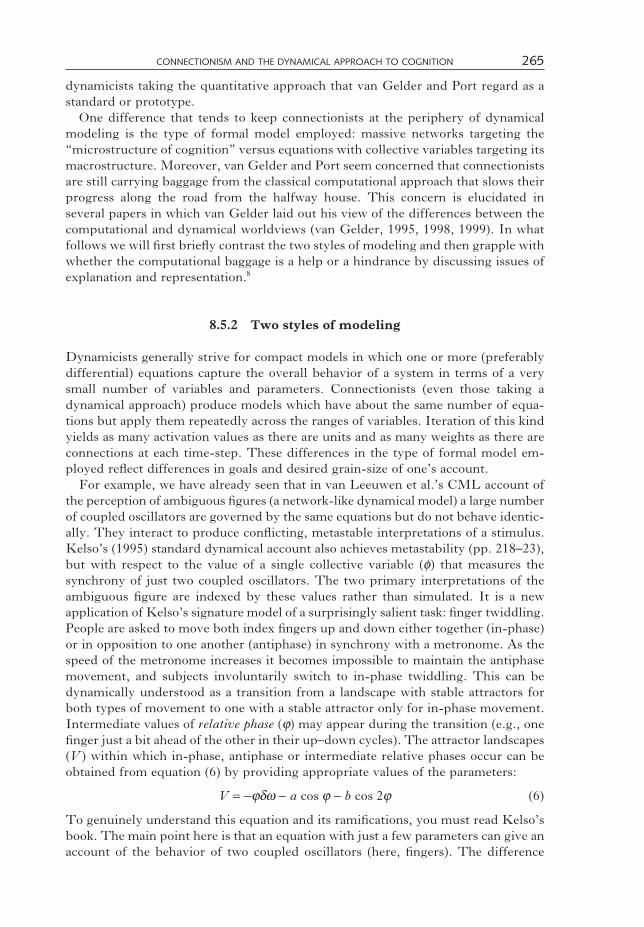
CONNECTIONISM AND THE DYNAMICAL APPROACH TO COGNITION 265
dynamicists taking the quantitative approach that van Gelder and Port regard as astandard or prototype.
One difference that tends to keep connectionists at the periphery of dynamicalmodeling is the type of formal model employed: massive networks targeting the“microstructure of cognition” versus equations with collective variables targeting itsmacrostructure. Moreover, van Gelder and Port seem concerned that connectionistsare still carrying baggage from the classical computational approach that slows theirprogress along the road from the halfway house. This concern is elucidated inseveral papers in which van Gelder laid out his view of the differences between thecomputational and dynamical worldviews (van Gelder, 1995, 1998, 1999). In whatfollows we will first briefly contrast the two styles of modeling and then grapple withwhether the computational baggage is a help or a hindrance by discussing issues ofexplanation and representation.8
8.5.2 Two styles of modeling
Dynamicists generally strive for compact models in which one or more (preferablydifferential) equations capture the overall behavior of a system in terms of a verysmall number of variables and parameters. Connectionists (even those taking adynamical approach) produce models which have about the same number of equa-tions but apply them repeatedly across the ranges of variables. Iteration of this kindyields as many activation values as there are units and as many weights as there areconnections at each time-step. These differences in the type of formal model em-ployed reflect differences in goals and desired grain-size of one’s account.
For example, we have already seen that in van Leeuwen et al.’s CML account ofthe perception of ambiguous figures (a network-like dynamical model) a large numberof coupled oscillators are governed by the same equations but do not behave identic-ally. They interact to produce conflicting, metastable interpretations of a stimulus.Kelso’s (1995) standard dynamical account also achieves metastability (pp. 218–23),but with respect to the value of a single collective variable (φ) that measures thesynchrony of just two coupled oscillators. The two primary interpretations of theambiguous figure are indexed by these values rather than simulated. It is a newapplication of Kelso’s signature model of a surprisingly salient task: finger twiddling.People are asked to move both index fingers up and down either together (in-phase)or in opposition to one another (antiphase) in synchrony with a metronome. As thespeed of the metronome increases it becomes impossible to maintain the antiphasemovement, and subjects involuntarily switch to in-phase twiddling. This can bedynamically understood as a transition from a landscape with stable attractors forboth types of movement to one with a stable attractor only for in-phase movement.Intermediate values of relative phase (ϕ) may appear during the transition (e.g., onefinger just a bit ahead of the other in their up–down cycles). The attractor landscapes(V) within which in-phase, antiphase or intermediate relative phases occur can beobtained from equation (6) by providing appropriate values of the parameters:
V = −ϕδω − a cos ϕ − b cos 2ϕ (6)
To genuinely understand this equation and its ramifications, you must read Kelso’sbook. The main point here is that an equation with just a few parameters can give anaccount of the behavior of two coupled oscillators (here, fingers). The difference

266 CONNECTIONISM AND THE DYNAMICAL APPROACH TO COGNITION
between the fingers’ spontaneous frequency and the metronome’s frequency is re-flected in δω. The a and b parameters reflect (indirectly) the oscillation frequency(how fast the fingers are moving), and a/b is a crucial coupling ratio (when it is small,oscillation is fast and in-phase movement is the only attractor). Certain combinationsof parameter values produce intermittency (the system fluctuates chaotically betweenthe two kinds of movement, which now are semi-stable rather than stable). Changethe realization of the equation from finger phases to competing interpretations of anambiguous figure (by changing the interpretation of each collective variable), andvoilà – equation (6) models a perceptual phenomenon (the distribution of switchingtimes) at an abstract level.
Van Leeuwen et al.’s CML model is different in part because it does two jobs.Unlike Kelso’s model, it simulates the percepts themselves – its units actually organ-ize themselves into synchronized columns or rows to simulate the two interpreta-tions of the ambiguous display. Like Kelso’s model, though, it also models themore global perceptual phenomenon of semi-stable interpretation by repeatedly butirregularly switching between these percepts.
This difference in style of modeling has other consequences. Certain concepts thatare part of the “computational baggage” (our metaphor) apply much more naturallyto dynamical network models than to standard dynamical models. In the ambiguousfigures task, van Leeuwen et al.’s explanation comes in the form of a mechanisticmodel, within which the metastable patterns can reasonably be regarded as twoalternative representations of the stimulus (albeit distributed rather than classical).Kelso’s compact system was not designed to do these jobs; it models the fluctuationbetween interpretations of the stimulus array but not the interpretations themselves.In taking a closer look at these computational concepts and at the dynamical alternat-ives, we will find that each can play a different but useful role in exploring dynamicalnetwork models.
8.5.3 Mechanistic versus covering-law explanations
The notions of mechanistic model and representation that we find useful in think-ing about dynamical network models are rooted in stronger, classical notions:homuncularity and symbolic representation. Van Gelder (1995, p. 351) had theclassical versions in mind when he characterized the computational approach interms of “a mutually interdependent cluster” of properties: “representation, com-putation, sequential and cyclic operation, and homuncularity.” A computer programwith subroutines is a prototype that gives a good, quick sense of what he means.Computation involves discrete operations that manipulate representations; theyapply sequentially (not in parallel); and sometimes a particular sequence of such op-erations will apply iteratively or recursively (cyclic operation – here a discrete notionthat is not to be confused with oscillation or limit cycles in a dynamical model).When combined with these other properties, representations are sequences of mani-pulable elements that usually also have meaning (are symbolic) – this special caseis the classical notion of representation. Before discussing representation further, wewill take a look at computational versus dynamical approaches to explanation andthe special case of homuncularity.
The homuncularity property derives from Daniel Dennett’s (1977) characteriza-tion of the components in a mechanistic model of the mind as homunculi. By this

CONNECTIONISM AND THE DYNAMICAL APPROACH TO COGNITION 267
metaphor – whimsical but making a serious claim – Dennett saw the mind as a com-mittee of little agents, each with its own specialized subtask (e.g., discrimination,memory, evaluation), who pass messages (representations) to one another to performthe overall task. Each little agent itself can be analyzed as a committee of somewhatmore specialized, less clever agents; and so forth until the lowest-level agents per-form primitive calculations such as picking the larger of two numbers. Put less color-fully, such a system has a hierarchy of components, each of which performs itssubtask by taking representations as input, operating on them, and sending theoutputs to other components.
A mechanistic model relaxes this characterization, such that in some cases thecomponents may function and interact continuously rather than discretely and theirinteractions may be better characterized as causal or information-bearing than asclassically representational. One way in which scientists construct such a model is tofirst decompose a task into subtasks and then try to recompose it by specifying thecomponent performing each subtask and its interactions with other components (seeBechtel and Richardson, 1993). The model is taken to provide an explanation of thesystem’s performance of the task. In principle the decomposition could continue downto primitives (cognitive models are often assumed to “bottom out” in neurobiology),but in practice modelers usually limit themselves to going down one or two levels. Whenthe components of a model like this can be localized in the system being modeled(e.g., identifying edge-detectors in the primary visual cortex), Bechtel and Richardson(1993) call them complex systems to distinguish them from simple systems (for whichcomponents have not been identified) and from integrated systems (in which the com-ponents interact by feedback loops or other reciprocal connections – the most difficultkind of model and usually not achieved until a research program reaches maturity).
Who needs mechanistic explanation? Most explanations in the mainstream ofbiology tend to be of this genre. Symbolic models in cognitive science generallyqualify – they served as Dennett’s paradigm case of homuncularity and van Gelder’sprime target. (However, competence models such as Chomskian grammars havea componential structure that may not map cleanly on to the processing systemmodeled). Standard dynamical models are generally claimed to bypass the mechan-istic style of explanation. It is network models for which the question gets mostinteresting, but to show why, we first need to ask: what are dynamical modelersdoing if not providing mechanistic explanations?
One possibility is that dynamicists merely describe a system by identifying regu-larities in its behavior. But van Gelder (1998, p. 625) rejected this suggestion, notingthat dynamical accounts of cognition are no different in form than dynamical ac-counts of physical phenomena such as planetary motion. Since the latter count asexplanatory, so should the former. Indeed, his point is well taken; the contrast is notbetween explanation and description, but rather between two forms of explanation.The logical positivists identified a form of explanation, deductive-nomological orcovering-law explanation, which fits the dynamicist case. In a covering-law explana-tion, a phenomenon is explained by showing how a description of it can be derivedfrom a set of laws and initial conditions. The dynamical equations provide the lawsfor such covering-law explanations, and by supplying initial conditions (values ofvariables and parameters), one can predict and explain subsequent states of thesystem. That is the appropriate kind of explanation for van Gelder, since he pro-poses to regard cognition solely as a dynamical system – one that changes states intime as expressed in equations.

268 CONNECTIONISM AND THE DYNAMICAL APPROACH TO COGNITION
Now we can consider networks. The simplest thing to say is that the type ofexplanation attributed to them can vary with the design of the network and with thedesigner’s leanings between classical connectionism and dynamicism. Much moreinteresting is the prospect that they may lead us to new kinds of explanation thatcombine and extend current options. Van Gelder (1995, p. 374) projected thatcombining ingredients of the two worldviews in connectionism “may well turn outto be an unstable mixture” and refrained from doing so; we prefer to focus on theconstructive synthesis that may emerge from the energy put into such a project.(Clark, 1997b, was similarly optimistic about combining these types of explanationand provided a thoughtful discussion of explanation more generally.)
Here are some cases. Sejnowski and Rosenberg’s (1986) NETtalk network canserve as an exemplar of a feedforward connectionist design, which in this caseprovides a mechanistic explanation of reading aloud (see section 3.2.2.3 for moredetails). At the first level down, it is easy to identify components (the input, hidden,and output layers) and to state they are connected by two full sets of feedforwardconnections. Below that there are two more levels of decomposition on the inputlayer (seven sets of letter units) and one more level on the output layer (one set ofarticulatory feature units). It is distinctive to connectionist networks that the hiddenlayer affords only a functional decomposition: cluster analysis reveals functionalcomponents for various grapheme–phoneme regularities, vowels vs. consonants, etc.The connectivity of the network is also highly distributed, unlike classical systems.The designers built the network as a mechanistic model, but cannot give a completemechanistic analysis of the microfeatures and microactivities that result from itsadaptive weight changes during learning. However, the incomplete mechanisticexplanation is the best available; dynamical analysis has little to offer towards under-standing feedforward networks.
When interactivity is added to layered networks of this type via recurrent connec-tions, complex activity extended across time and connections becomes very important.This aspect of a network model benefits from dynamical analysis. We suggest that aconnectionist dynamical approach offers the opportunity to embrace both types ofexplanation and use them to serve complementary purposes (see Bechtel, 1998). Mostsimply, the dynamical analysis can offer covering laws that characterize overall pat-terns of change in a system (generally in terms of aggregate or external variables), andthe mechanistic one can show how those changes are effected. The connectionistresearcher built the network, knows its components and how they are connected, andcan use this knowledge to “go behind the scenes” and provide a (partial) mechanisticaccount of the phenomena captured in the dynamical covering-law explanation of thesystem. Dynamical tools may then be used not only to characterize the complete system,but also the interaction of the components. For example, in building the CMLmodel of ambiguous figure perception, van Leeuwen et al. (1997) knew from Kelso’swork that two coupled oscillators could produce the right kind of semi-stable beha-vior. They wanted to build a system at a much finer grain to model the microstructureand microactivity underlying the percepts themselves in addition to the overall semi-stable behavior. Their novel solution (using a large number of coupled oscillators ascomponents) was informed by the prior dynamical model but extended it significantlyby treating component parts as dynamically interacting oscillators. The resulting CMLmodel is best described using a combination of dynamical and mechanistic analysis.
In another example from this chapter, a mechanistic analysis gets even further withSkarda and Freeman’s (1987) model of the olfactory bulb. Built at an intermediate

CONNECTIONISM AND THE DYNAMICAL APPROACH TO COGNITION 269
grain-size, the “units” were just 16 large nervous system components that were lesshomogeneous than the units of a connectionist network; for example, all of theexcitatory (pyramidal) cells of the anterior olfactory nucleus were represented collect-ively in one component. However, their interactive connections produced complexbehavior in the network as a whole. Dynamical concepts and analysis were crucialfor understanding the chaotic and limit cycle behavior that emerged. Anotherexample: Beer’s autonomous controller network for insects’ tripod gait has six replica-tions of the same five units (a componential organization at this level). Three of theunits controlling each leg have well-defined subtasks (each clearly controls its ownspecialized motor effector) but are dynamical in their quantitative states and intercon-nected activity (including influence from the other two units – the interneurons).Each leg’s activity is best understood in terms of a limit cycle, but the state space isdefined with respect to components of the network.
The ability of these two perspectives to complement each other becomes even moreevident when dynamical analysis is applied not only to the whole network but also tosome of its components. This can work even in a network with thoroughly homo-geneous units within each layer. An interesting case covered above is that of Elman(1991), who knew the gross architecture of his simple recurrent network (SRN) forpredicting words in sentences and could give a rough mechanistic account based onhis own design work. However, he also used principal components analysis (a toolfrom yet another tradition, multivariate statistical analysis) to identify functionalcomponents of the system on the hidden layer and used DST tools to discoverexactly what task those components were accomplishing. For example, plottingtrajectories through the state space of components 1 and 11 revealed the phenom-enon that relative clauses were being wrapped corkscrew-like into the space.
It is not known to what extent an orchestration of methods like this might yieldinsight into large networks with more complex interactions among units. MichaelWheeler (1998) considered the difficulty of explaining the activity of networksexhibiting what Clark (1997a, pp. 163–6) called “continuous reciprocal causation.”An example is Beer’s nonautonomous control network, in which sensor input com-pletes a loop between the controller and the environment, but Wheeler was mostconcerned about larger, more homogeneous networks and especially those in evo-lutionary robotics (see sections 9.4 and 9.5) whose organization is minimally con-strained by human preconceptions of design. He thought the explanatory stancemust become more holistic as the amount of continuous reciprocal causation in-creases, shifting away from modular (mechanistic) explanation and towards systemdynamics. “The justification for this claim is that the sheer number and complexityof the causal interactions in operation in such systems force the grain at which usefulexplanations are found to become coarser” (Wheeler, in press, p. 16). Clark (1997a,p. 175) had a similar concern but argued for proceeding more optimistically, “add-ing new tools to cognitive science’s tool kit, refining and reconfiguring but notabandoning those we already possess. After all, if the brain were so simple that asingle approach could unlock its secrets, we would be so simple that we couldn’t dothe job!”9
In accord with the more optimistic view of Clark, we look forward to seeing howmuch headway can be made, even with highly interactive networks, when mechan-istic and dynamical explanation are combined and extended. However, it is so earlyin dynamical network research that this suggestion of complementary, even integ-rated, use of two kinds of explanation must be tentative. Those who wish to use an

270 CONNECTIONISM AND THE DYNAMICAL APPROACH TO COGNITION
exclusively dynamical approach to cognition may find their own way to go behindthe scenes, in some way parsing the system and building a hierarchy of dynamicalmodels that cover a variety of grain-sizes from the overall phenomenon of intereston down. In his 1995 book, Kelso sketched such a vision in chapter 2 and consideredmodeling at neuronal levels in chapter 8. He emphasized, though, that his equationsgive a different parsing than does a mechanistic analysis of the biological systemsthat realize them. For now, networks of homogeneous units and connections, eachwith its own application of the equations governing the system, do a modeling jobthat is hard to replace by purely dynamical analyses. Can we do better than simplyperforming each kind of analysis separately? It would be most interesting if attemptsto grapple with these problems led to new notions of explanation within the philo-sophy of science in addition to better models.
8.5.4 Representations: Who needs them?
We turn now to a second area of discrepancy between connectionist and dynam-ical approaches that places those who seek to combine them at the periphery ofdynamicism (but perhaps at the leading edge of the future of cognitive modeling):the role of representations. Disagreements about representation abound. It is leasttroublesome within the symbolic approach, where the notion that cognition involvesoperations upon representations (construed as structured sequences of symbols) iscentral. At the other end of the road, among those dynamicists who attend to theconcept of representation at all, it tends to be either denied or radically redefined.Between these extremes are the connectionists, who see part of their mission as (lessradically) redefining representation. Activation patterns across the layers of a net-work are commonly (though not universally) regarded as “subsymbolic” (Smolensky,1988) – a departure from symbols in their fine grain, their status as numerical vectors,and the kinds of activity that generate them (parallel processing, and for interactivenetworks, settling into attractors or other kinds of change across a nontrivial tem-poral dimension). However, van Gelder and Port (1995) worried that connectioniststaking this view (especially those working with feedforward networks such asNETtalk) have insufficiently shed notions of representation rooted in the symbolicapproach. On this view, an unchanging composition of subsymbols is in danger ofbeing treated as a static symbol.
Dynamical reappraisals of representation were considered as part of an argumentfor the dynamical hypothesis by van Gelder (1998; quotes from p. 622). His startingpoint was to unequivocally dispense with “static configurations of symbol tokens” –a core commitment of what he calls the computational view (some of the commentatorson this BBS paper, seeing computation as broader, would prefer a different term).The main alternative he noted is that dynamicists “find their representations amongthe kinds of entities that figure in DST, including parameter settings, system states,attractors, trajectories, or even aspects of bifurcation structures” and eventually “evenmore exotic forms.” (See also van Gelder and Port, 1995, p. 12.) That he felt nourgency to pare down this mixed bag of possibilities reflects the fact that few if anydynamicists view representation as a core concern. Indeed, van Gelder also noted(refraining from endorsement or disapproval) the more radical view that dynamicistscan develop models of cognition that “sidestep representation altogether.”10 He citedthe work by Beer and by Skarda and Freeman (discussed above in sections 8.3.1 and

CONNECTIONISM AND THE DYNAMICAL APPROACH TO COGNITION 271
8.4.1) as exemplifying the ability “to imagine how any nonrepresentational systemcould possibly exhibit cognitive performances” and also to model such a system.
One could quibble about whether models of sensorimotor function are a sufficientbasis to argue that cognition more generally can be modeled nonrepresentationally;yet, they give a toehold. Freeman and Skarda (1990) clearly endorsed the positionthat representation can be dispensed with (at least in dynamical models of perceptiongrounded in brain function) in a commentary with the title “Representations: Whoneeds them?” They answered: “Functionalist philosophers, computer scientists, andcognitive psychologists need them, often desperately, but physiologists do not, andthose who wish to find and use biological brain algorithms should also avoid them”(p. 379). Why should they be avoided? “[T]he idea of representation is seductive,”giving “the illusion that we understand something that we do not” but in fact “isunnecessary to describe brain dynamics” and even “impedes progress” (pp. 375–6).In illustration they gave this remarkable reprise of their olfactory bulb work (notethat the “burst” they refer to is a spatial pattern of activity across the entire bulbunder the control of one of the cyclic attractors sketched in figure 8.7):
For more than 10 years we tried to say that . . . each burst served to represent the odor-ant with which we correlated it. . . . This was a mistake. After years of sifting throughour data, we identified the problem: it was the concept of representation. . . . [Theyexplain that the pattern for a given odor occurs only under conditioning and changes ifthe reinforcement contingency is altered or a new odor is added.] Our findings indicatethat patterned neural activity correlates best with reliable forms of interaction in acontext that is behaviorally and environmentally co-defined by what Steven Rose (1976)calls a dialectic. There is nothing intrinsically representational about this dynamic pro-cess until the observer intrudes. It is the experimenter who infers what the observedactivity patterns represent to or in a subject, in order to explain his results to himself(Werner, 1988a, 1988b). (Freeman and Skarda, 1990, p. 376)
They further stated that this insight led them to ask new questions of their data andthat their dynamical network model, with its emphasis on the role of chaos, was oneof the novel answers that resulted.
Skarda and Freeman’s network was intended to model an actual biological sys-tem. Researchers in the field of artificial life (the topic of chapter 9) attempt a moreabstract characterization of such biological constructs as evolution, sensation, andmotor control, and many of them share the skepticism about representation. Forexample, speaking from his experience with autonomous agents (including his insectcontroller networks), Beer (1995, p. 144) concluded that generally “there need be noclean decomposition of an agent’s dynamics into distinct functional modules and noaspect of the agent’s state need be interpretable as a representation.” Philosophersfocusing on evolutionary robotics, including Beer’s work, have launched into amajor re-examination of the notion of representation. Wheeler (1998), writing aboutsystems that exhibit high degrees of continuous reciprocal causation, assumed thathis arguments against their homuncularity (and more generally, their modularity)counted as well against their having representations. (He argued elsewhere the pointthat makes this plausible: the claim that these properties are mutually supportive.)This was a soft rather than hard conclusion; for example, he left open the possibilitythat more sophisticated evolved robotic control systems of the future would be moredecomposable. Clark (1997a; all quotes from pp. 174–5) agreed that such systemspresent the “most potent challenge” in finding a role for internal representation, but

272 CONNECTIONISM AND THE DYNAMICAL APPROACH TO COGNITION
again preferred a more optimistic and inclusive stance. First, in coming to grips withsuch complex dynamics, “the notion of internal representation itself may be subtlytransformed,” losing some of its classical connotations while co-opting dynamicalnotions of inner events (chaotic attractors, trajectories in state space, and so forth;a list similar to van Gelder’s). But Clark equally threw down the gauntlet todynamicists:
The recent skepticism concerning the role of computations and representation in cognit-ive science is, I believe, overblown. . . . The minimal conditions under which internalrepresentation talk will be useful, I have argued, obtain whenever we can successfullyunpack the complex causal web of influences so as to reveal the information-processingadaptive role of some system of states or of processes. . . . [C]ontinuous reciprocal causa-tion between internal and external factors . . . appears unlikely to characterize the rangeof cases for which the representational approach is in any case most compelling–viz.,cases involving reasoning about the distant, the nonexistent, or the highly abstract. Insuch cases, the focus shifts to the internal dynamics of the system under study. Thecrucial and still-unresolved question is whether these internal dynamics will themselvesreward a somewhat more liberalized but still recognizably representation-based under-standing. . . . no alternative understanding of genuinely representation-hungry prob-lem solving yet exists, and . . . it is hard to see how to give crisp, general, and perspicu-ous explanations of much of our adaptive success without somehow reinventing theideas of complex information processing and of content-bearing inner states.” (Clark,1997a, pp. 174–5)
So far we have looked at how the notion of representation has fared when confrontedwith biological systems and with their simulated counterparts, evolved robot con-trollers. Van Gelder added industrial machinery to the array of test cases in a 1995article, “What might cognition be, if not computation?” His general goal was toargue that dynamical systems provide a plausible alternative to computational ones,and that such systems need not have representations. Although at some points in thepaper he focused on a classical computational definition of representation, he alsosaid that his arguments should go through using “pretty much any reasonable char-acterization, based around a core idea of some state of a system which, by virtue ofsome general representational scheme, stands in for some further state of affairs,thereby enabling the system to behave appropriately with respect to that state ofaffairs” (van Gelder, 1995, p. 351; he adapted this characterization from Haugeland,1991). This definition of representation is broad enough to cover both classicalsymbolic and connectionist subsymbolic approaches.
The notion of “stands in for” requires some explication. One way to characterizeit is in terms of carrying information: one state or event can stand in for another if itcarries information about that other state or event. The notion of carrying informationabout something is usually explicated in terms of causal relations (Dretske, 1988).But this notion of information is both too general and too narrow for explicatingrepresentation. It is too general because any effect carries information about its cause,but not every effect constitutes a representation. It is too narrow because it fails toaccount for misrepresentation – the possibility that some state might falsely representsomething else when it was not caused by it. Based on this and other arguments,Millikan (1993) proposed that we need to look in a different direction, specifically, atthe agent or device that uses (consumes) the information. If a consumer Z is designed(e.g., by evolution or by an engineer) to use Y to carry information about X, then Y

CONNECTIONISM AND THE DYNAMICAL APPROACH TO COGNITION 273
might serve as a representation of X even if Y never actually carries informationabout X. For example, a radiation detector (Y) may have been designed for a plantsupervisor who wants to be informed if there is ever a radiation leak (X). If no leaksoccur, it will in fact produce only false alarms; nonetheless, the radiation detectorserves to represent radiation leaks.
In practice, we generally need to look in both directions: some state is a repres-entation only if it is used to gain information about something else, but we identifywhat it represents by determining what is capable of bringing it about. For example,in Lettvin et al.’s (1959) classic identification of ganglion cells in the frog’s retina asbug detectors, two kinds of findings jointly were needed to determine what the firingof these cells represented: (a) increased firing of these cells generated bug-eatingbehaviors in the frog; (b) bug-like shapes generated increased firing. There are,therefore, three interrelated components in a representational story: what is repres-ented (bugs), the representation (increased firing of ganglion cells), and the user ofthe representation (the frog, or the frog’s action system).
While this is not a complete characterization of representation, it provides a suf-ficient foundation to begin considering van Gelder’s contention that dynamical sys-tems need not have representations. To make his case, van Gelder reached back overtwo centuries to James Watt’s groundbreaking design for using a steam engine topower machinery via a flywheel, and suggested that its centrifugal governor wouldbe “preferable to the Turing machine as a landmark for models of cognition” (vanGelder, 1995, p. 381). The governor was the second of two major innovations neces-sary to the invention’s success. Watt’s first innovation was a gearing system thatallowed an oscillating piston to drive a rotating flywheel. But the solution to theproblem of translating one kind of motion into another raised a second problem:how to maintain a constant flywheel speed in the face of constantly fluctuating steampressure as well as resistance due to workload on the machinery being driven by theflywheel. (For many kinds of machinery, such as industrial weaving machines, it isimportant that a constant speed of operation be maintained, despite fluctuations inresistance, via constant flywheel speed.) The speed at which the flywheel turns canbe reduced, when necessary, by partly closing a valve to reduce the amount of steamcoming through the pipe leading from the boiler to the piston. Similarly, partlyopening the valve increases the amount of steam. But who or what would keepadjusting the valve?
Watt’s solution borrowed a technology already employed in windmills; it is shownpictorially in figure 8.9(a) and schematically in figure 8.9(b). (The pistons and gear-ing system between the valve and flywheel are not shown, but complete the loop.)To create a governor, he attached a vertical spindle to the flywheel which wouldrotate at a speed proportionate to that of the flywheel, and attached to the spindletwo arms with metal balls on their ends. The arms were free to rise and fall as aresult of centrifugal force. Through a mechanical linkage, the angle of the armswould change the opening of the valve, thereby controlling the amount of steamdriving the piston and hence the rotational speed of the flywheel itself.
As a first step towards establishing the plausibility of the idea that cognitivesystems, construed as dynamical systems, lack representations, van Gelder arguedthat the Watt governor operates without representations. He called “misleading” “acommon and initially quite attractive intuition to the effect that the angle at whichthe arms are swinging is a representation of the current speed of the engine, and itis because the arms are related in this way to engine speed that the governor is able

274 CONNECTIONISM AND THE DYNAMICAL APPROACH TO COGNITION
Consumer
Valve(opening)
Flywheel(speed)
Spindle arms(angle)
Representation
steam pressure +–
– +spindle turning
linkage – +mechanism
Machinery
powerresistance
Referent
(b)
Flywheel
Arms
Linkage mechanism
Valve
(a)
Figure 8.9 Watt’s centrifugal governor for a steam engine. (a) Drawing from J. Farley,A Treatise on the Steam Engine: Historical, Practical, and Descriptive (London: Longman,Rees, Orme, Brown, and Green, 1927). (b) A schematic representation showing that theangle of the spindle arms carries information about the speed of the flywheel for the valve,which uses the angle to determine the opening, thereby regulating the speed of the flywheel.
to control that speed” (van Gelder, 1995, p. 351). He offered several arguments fornot construing the angle of the arms as representations; here we suggest counter-arguments to two of them (for a fuller discussion of these and the other arguments, seeBechtel, 1998). Van Gelder began by contending that there is no explanatory utilityin describing the angle of the arms in representational terms (that is, the dynamicalanalysis is sufficient). To establish explanatory utility, we must argue that (a) amechanistic analysis is informative, and (b) that analysis includes a particular repres-entational story about the arm angles: they stand in for the speed of the flywheel andcan regulate the valve opening because they carry this information.
First, then, here is a brief mechanistic analysis of the Watt governor (see Bechtel,1999). It has several different parts, including the flywheel, the spindle and arms, anda linkage mechanism connected to a valve. As figure 8.9(b) makes clear, each compon-ent operates on a different engineering principle and hence performs a specific subtask;each subtask contributes to the overall task of the system via the component’sconnection with the next component in the loop. That is, the opening of the valve getstransformed (via the piston) into the rotation of the flywheel, which gets transformedinto the angle of the spindle arms, which gets transformed into the opening of thevalve. In this way, we have shifted vocabularies from one describing the overall beha-vior of the Watt governor to one describing what its parts do. Then there is an extrastep back up to the system level by connecting the task of each component to theneeds of the whole system. Here it becomes clear why Watt inserted the spindle arms.It is because the spindle arms rise and fall in response to the speed of the flywheelthat their angle can be used by the linkage mechanism to open and shut the valve.Without the spindle arms and their linkage mechanism, the valve has no access toinformation about the flywheel speed. They were inserted in order to encode thatinformation in a format that could be used by the valve-opening mechanism.
This makes the spindle arm angle an instance of a more general point about rep-resentation: typically someone (a designer, or evolution, or the particular consumerproduced by design or evolution) has gone to the trouble of representing a state ofaffairs in another medium because the representational medium is more suitable for

CONNECTIONISM AND THE DYNAMICAL APPROACH TO COGNITION 275
use by the consumer. This can be due to its format, its accessibility (e.g., wordsare generally more accessible to our cognitive system than are their referents), theefficiency with which it can be manipulated (e.g., computer-aided design), economy(e.g., industrial prototypes), and so forth. The representation is not just one vertexof the triangle in figure 8.9(b), a part like any other part of the dynamic loop; it wasinserted to play a particular (representational) role and the system functions becauseit was designed appropriately for that role.
Another of van Gelder’s arguments “for supposing that the centrifugal governoris not representational is that, when we fully understand the relationship betweenengine [flywheel] speed and arm angle, we see that the notion of representation isjust the wrong sort of conceptual tool to apply” (van Gelder, 1995, p. 353). Because“arm angle and engine speed are at all times both determined by, and determining,each other’s behavior” the relationship is “much more subtle and complex . . . thanthe standard concept of representation can handle.” Here is Clark’s continuous recip-rocal causation again, but the complexity resides only in the dynamical analysis. Itis quite possible, and desirable, to undertake a complementary classical analysis.As just noted, it (a) identifies the system’s components, the subtasks they perform,and their connectivity, and (b) picks out the spindle arm angle as representing theflywheel’s speed for use by the valve. It happens in this case that something isstanding in for something else by being coupled to it in a dynamical manner. Thisopens the way to a dynamical analysis that makes use of the identified components,but emphasizes their coupling and provides equations that provide an elegant andspecific account of their state changes in time. Within the confines of this dynamicalanalysis the components form a loop in which no one of them is viewed as providinga starting point, let alone a differentiated role such as referent or representation. Ifthe equations can be uncovered, this analysis yields an elegant covering-law explana-tion of the dynamics of that loop–no more and no less.
In analyzing the Watt governor in this way, we have taken the position thatrepresentations should be construed broadly rather than restrictively. They can bedynamic rather than static; vary continuously in time rather than discretely; andinvolve quantitative operations rather than sequential manipulations of symbols.The important thing is that something is standing in for something else. Generaliz-ing the lessons learned from the Watt governor to biological or artificial agents, itwould seem that they can coordinate their behavior with an environment becausecomponents of these agents vary their states in response to the environment so as tostand in for it. Without such representations, it seems difficult to explain how thesystem is able to take into account specific features of the environment. We shouldemphasize that this does not require that the system build up a complete repres-entation of its environment. Theorists such as Ballard (1991) and Churchland,Ramachandran, and Sejnowski (1994) have argued that we only selectively, andactively, sample the environment. Whatever information we do sample, however,must ultimately be represented within the system in order to be employed in coor-dinating behavior.
De-emphasizing the importance of the quantitative status of a system turns out tobe helpful in characterizing dynamical analysis as well. Rick Grush pointed out in areview of Port and van Gelder’s 1995 book that “A large portion of the models of‘higher’ cognitive processes articulated in the book have exactly the same processing-step character as the vilified computational alternatives, even though the language,mathematics, and illustrations used to present the models obscure this fact” (Grush,

276 CONNECTIONISM AND THE DYNAMICAL APPROACH TO COGNITION
1997b, p. 235). Where equations were supplied, that is, they tended to be differenceequations by which the value of a variable at time t + 1 depends on that variable andothers at time t. This is no closer to real time than the processing steps of a classicalAI model. In responding to this argument, van Gelder (1999, p. 8) arrived at a morerealistic way of distinguishing types of models. “In dynamical models, there aredistances in state, and distances in time, and both are systematically related to thebehavior of the system.” It is the geometry of state spaces in relation to time (whetherdiscrete or continuous) that best characterizes dynamical analysis. This also suggeststhat the suitability of dynamical analysis for a particular network has more to dowith whether trajectories in state space capture something important than with thefact that their representations are quantitative vectors rather than symbol strings.That sounds just right.
8.6 Is Dynamicism Complementary to Connectionism?
Terence Horgan and John Tienson (1996) presented a very specific vision of howconnectionism and DST can collaborate in providing an alternative to classicism.They unfolded it by first characterizing the classical approach in terms of DavidMarr’s (1982) well-known three levels of description and then adding five specificassumptions of classicists regarding these levels. Essentially, this is the same startingpoint as van Gelder and Port’s computational approach, although in the end Horganand Tienson rejected less of it. In summarizing their framework here, we primarilyuse their terminology and their characterization of classicism but also (in paren-theses) show Marr’s way of referring to each level.
Level 1: Cognitive-state transitions (Marr: an abstract theory of the computation)A cognitive-transition function (CTF) maps one total cognitive state (TCS) to thenext; that is, it specifies input–output mappings of intentional states. The choice offunction depends in part on the goal of the computation. The CTF is regarded astractably computable because, classically, general psychological laws reduce whatwould otherwise be a brute list of mappings (see assumption 5).
Level 2: Mathematical-state transitions (Marr: an algorithmic specification of thecomputation) An algorithm is chosen to realize the level-1 input–output mapping(CTF) and representations are chosen for the input and output. Classically, formalrules (see assumptions 2 and 3) manipulate syntactically structured sequences ofsymbols (see assumptions 1 and 4).
Level 3: Physical implementation (Marr: implementation) The level-2 com-putations are realized (implemented) in a physical system. A particular machinelanguage program run on a particular digital computer is the best exemplar, bothgenerally and for classicists.
Horgan and Tienson then identified the five key assumptions of classicism. Assump-tions 1–3 give the basic layout of level-2 rule-governed symbol manipulation (3 is astronger version of 2 and implies it; both imply 1). Assumption 4 makes languageor language-like processing a special case (it is a stronger version of 1 and impliesit, but leaves room for imagistic processing, for example, to satisfy 1 but not 4).Assumption 5 asserts the fundamentally computational worldview, which the other

CONNECTIONISM AND THE DYNAMICAL APPROACH TO COGNITION 277
assumptions elaborate, and also makes a specific claim that it is realizable within avail-able resources. Retaining the numbering and wording of the assumptions (pp. 24–5)but labeling and rearranging them for easy reference:
Fundamental computational assumption (level 1):(5) Human cognitive transitions conform to a tractably computable cognitive-transition function.
Representation (level 2):Weak (1) Intelligent cognition employs structurally complex mental
representations.Strong (4) Many mental representations have syntactic structure.
Processing (level 2):Weak (2) Cognitive processing is sensitive to the structure of these representa-
tions (and thereby is sensitive to their content).Strong (3) Cognitive processing conforms to precise, exceptionless rules, statable
over the representations themselves and articulable in the format of acomputer program.
In evaluating these five assumptions for their own (nonclassicist) purposes, Horganand Tienson made a provocative cut: in addition to retaining the weakest assump-tions about representation and processing, they also argued for retaining the strongassumption that representations can be syntactically structured. They picked out“hard” rules (algorithms) and computational tractability as classicism’s points ofvulnerability. Hence, in arguing for an alternative to classicism, they retained as-sumptions 1, 2, and 4 and denied assumptions 3 and 5. Their favored alternative wasa dynamically oriented connectionism, which they viewed not as a half-heartedhalfway house but rather as the kind of dynamicism that is needed for the job ofmodeling cognition.
These choices put Horgan and Tienson into several different fights, not just withclassicists but also with most connectionists and most dynamicists. Horgan andTienson took issue with classicists over assumptions 3 and 5 (by rejecting hard rulesand expressing extreme skepticism that cognition could be computationally tract-able). They stood with their fellow connectionists in rejecting hard rules (the gen-eral arguments are covered at length in chapter 5 and need not be reviewed here).But their insistence that there is indeed a language of thought, and that its syn-tactic structure must in some way be represented, placed them in opposition tomany connectionists (see chapter 6). Finally, dynamicists should applaud Horganand Tienson’s rejection of assumption 5 but would tend to agree with van Gelderand Port that connectionist networks are a rather marginal medium for dynam-ical modeling (especially if they are viewed as realizing syntactically structuredrepresentations).
Horgan and Tienson dealt with the nay-sayers in two ways: argumentatively bydissecting and debating each assumption and positively by trying to entice them intothe alternative framework that they called noncomputational dynamical cognition (wewill simply call it dynamicism). To make the contrast with classicism clear, theyconstructed a noncomputational dynamical reconstrual of Marr’s three levels. Theirclaims at each level can be summarized as follows (see their pp. 63–4 for moredetail):

278 CONNECTIONISM AND THE DYNAMICAL APPROACH TO COGNITION
Level 1: Cognitive-state transitions In dynamicism the cognitive system isviewed as having general dispositions to move from one total cognitive state toanother, and these dispositions are captured in psychological laws that are softrather than general. There is no need for a tractably computable cognitive-transitionfunction.
Level 2: Mathematical-state transitions Total cognitive states are realized aspoints in the state space of a dynamical system, and transitions between states arerealized in trajectories through that state space. Each representation is a point (orregion), but not every point is a representation. Relations between syntactic struc-tures (e.g., sentences with vs. without a direct object) are captured not in the pres-ence or absence of certain steps in the algorithm generating a tree but rather in therelative positions of points. The discrete mathematics of algorithms is replaced bythe continuous mathematics of dynamical systems theory. More specifically, givenhow the dynamical system is implemented at level 3, it is a high-dimensional activa-tion landscape in which each dimension corresponds to the range of possible activa-tion values of one unit in a network.
Level 3: Physical implementation The dynamical system is implemented in aneural network of some sort (working hypothesis: a connectionist network). “Pointsin the state space of a dynamical system are realized by total activation patterns inthe associated network” (p. 64).
Horgan and Tienson’s denial of assumption 5 (the need for a tractably computablefunction) involves a distinction between computable and tractably computable. Onecould ask whether or not the cognitive transition functions that classicists attempt torealize in algorithms are actually computable (e.g., by a universal Turing machine).But to Horgan and Tienson, this was not the real issue. A cognitive system whosetransitions are computable but intractable is as nonrealizable as one whose transi-tions are noncomputable. Any actual cognitive system must be realizable in a phys-ical system that can implement mappings efficiently and quickly enough to be usable.They noted that tractable computation of this kind is far from guaranteed:
[T]here are infinitely many functions [even] with finite domain and range that are nottractably computable. Consider, for example, any googolplex of unrelated pairings. (Agoogolplex is 1 followed by 10100 zeros.) The difference between infinite and huge-but-finite is not important for cognitive science! (Horgan and Tienson, 1996, p. 26)
Classicists purport to get into the small-and-finite range by means of general psy-chological laws which reduce what would otherwise be a brute list of mappings “ toogargantuan” to specify. Horgan and Tienson presented arguments that laws of theright sort for a computational system (hard laws) are not what the cognitive systemconsists in, nor are they implemented by hard rules at the algorithmic level. On theirview, the way the cognitive system actually is built does not involve computation(the discrete mathematics of algorithms), so the tractability question does not evenarise.
Instead of general laws, Horgan and Tienson claimed that cognition has an iso-tropic and Quinean nature that makes computation untractable if not impossible.The problem of isotropy is that of gaining access to the right information for solvinga given task from all of the information in the system, while the Quinean problem

CONNECTIONISM AND THE DYNAMICAL APPROACH TO COGNITION 279
concerns measuring the appropriate characteristics of the whole network of beliefs(e.g., its coherence) so as to determine how to revise beliefs. They credited Fodor withrecognizing that these problems, originally identified in the context of confirmingscientific hypotheses, extend to the general task of belief fixation faced regularly bycognitive systems. They did not see Fodor, or anyone else, as having shown how aclassical system can overcome these challenges so as to handle a new input appropri-ately and efficiently: “Not only do we have no computational formalisms that showus how to do this; it is a highly credible hypothesis that a tractable computationalsystem with these features is not possible for belief systems on the scale possessed byhuman beings” (p. 42). One avenue of response would be to deny that these areproblems that need to be solved. Waskan and Bechtel (1997) contended that cogni-tion is far less isotropic and Quinean than suggested by Fodor or Horgan andTienson. A system with some degree of modularity (in the weaker sense exemplifiedin chapter 7, not Fodorian modularity) can concentrate its resources within a smallpart of the overall system. Rather than exhibiting an overall property of isotropy, forexample, in such a system finding the right information quickly will depend onwhether the right module is active (and in fact, humans not infrequently do fail toaccess relevant information that is somewhere in the system). A different avenue ofresponse was preferred by Horgan and Tienson: they claimed that noncomputationaldynamical cognition could easily be isotropic and Quinean. The problem of how tocompute in such an environment (a version of the tractability problem) does notarise if the system does not compute.
In characterizing their noncomputational dynamical conception of cognition,Horgan and Tienson retained the commitment to syntactic structure that is a legacyof the symbolic approach (as stated in assumption 4). They construed as mistakenthe common view that one of connectionism’s contributions is to repudiate the useof syntactically structured representations in cognitive models. As Horgan pointedout, instead of improving on classical symbolic accounts this move produces “aseriously crippled cousin of classicism.” He asked:
What exactly are we supposed to be gaining, in terms of our abilities to model cognitiveprocesses, by adopting an approach which (i) retains the assumption that cognitiveprocessing is representation-level computation, but (ii) eschews one extremely power-ful way to introduce semantic coherence into representation-level computation: viz., viathe syntactic encoding of propositional content? Qua representation-level computation,it looks as though this amounts to trying to model semantically coherent thought pro-cesses with one hand – the good hand – tied behind one’s back. (Horgan, 1997, p. 17)
It quickly becomes apparent, however, that their construal of syntax is one thatmany connectionists – but no classicists – would find comfortable. They pointed toPollack’s RAAM networks as exemplifying how to get syntactically structuredrepresentations in a noncomputational cognitive system. These are the same rep-resentations that we characterized in section 6.3 as exhibiting only functional com-positionality, in contrast to the explicit compositionality of symbolic representations.What makes RAAM representations functionally compositional is that there is usableinformation in them about the constituent structure of the tree from which theywere generated. However, neither Pollack nor Horgan and Tienson have probed todiscover how much syntactic information is represented nor for what range of lin-guistic performances it is adequate (beyond the passive transformation). They also

280 CONNECTIONISM AND THE DYNAMICAL APPROACH TO COGNITION
have not pursued in any detail how the dynamical level of analysis contributes (thoughwork by Elman and Christiansen suggests such a pursuit would be rewarding).
8.7 Conclusion
Cognitive scientists, including connectionist modelers, increasingly are employingdynamical concepts and the tools of DST. In this chapter we have seen how someresearchers have plotted trajectories through state space and identified differenttypes of attractors to better understand how their interactive networks did their job,and others have incorporated concepts such as chaos even at the design stage of theirresearch. But some advocates of a dynamical approach to cognition claim that muchmore is at stake than the introduction of new tools. Van Gelder and Port (1995)contended that dynamics offers a paradigm for cognitive science that promises toreplace both the symbolic and connectionist approaches. We examined critiques ofmechanistic explanation and representation and concluded that these concepts neednot be discarded (e.g., mechanistic explanation is complementary to the coveringlaw explanations of dynamicism). Finally, we provided an overview of Horgan andTienson’s version of a dynamical approach to cognition, which was friendlier thanvan Gelder and Port’s version with respect to both connectionist networks and thesymbolic notion that representations have syntactic structure. We did not agree withall their claims, but their placement of dynamical and connectionist approaches attwo different levels of a Marr-style analytic framework is a good starting point forworking out how these approaches can complement each other.
NOTES
1 A simulator for running Lotka–Volterra equations developed by Hendrik J. Blok isavailable free at http://www.physics.ubc.ca/~blok/files.html.
2 Of course, (c) also has starting points that are already on the cycle, and it is one of thedefining characteristics of an attractor that trajectories beginning at those points willremain within it. These special trajectories have no transients. Although the cycle in (a)exhibits this characteristic, it lacks another defining characteristic of attractors, the tend-ency to attract nearby trajectories. Thus, none of its trajectories have transients.
3 Interestingly, it does not much disturb encoding of the matrix (outer) clause; the threerelevant points are similar to those in figure 8.6(a). This may be a leaky network analog to“popping” the push-down stack in a standard symbolic parser.
4 This sensitivity is important, because pairs of words such as boy and boys were givenunrelated encodings on the input layer. The hidden layer seems to have extracted thesystematic contrast between singular and plural (as well as the essentials of subject–verbagreement) purely from distributional information in the corpus. The principal compon-ents analysis not only provides evidence of the network’s systematization of number butalso localizes identification of subject noun number in component 2 – an impressivecontribution to understanding how the network performs its task.
5 A weight space with an error dimension yields a very detailed display of its attractors –not just their locations but also their relative depths along the error surface. Occasionallyactivation spaces are plotted with an energy dimension included to obtain the sameeffect, as in figure 8.7 in section 8.4.1 (reprinted from Freeman, 1987).

CONNECTIONISM AND THE DYNAMICAL APPROACH TO COGNITION 281
6 Understanding why the system behaves in this way requires considerably more depth inDST than our brief introduction can provide. To pursue this elsewhere, a reader shouldpay particular attention to the tangency of stable (attracting) and unstable (repelling)directions at saddle nodes; to obtain intermittency, the system must be nudged to near-tangency. “When the saddle nodes vanish, indicating loss of entrainment, the coordina-tion system tends to stay near the previously stable fixed point. It’s as though the fixedpoint leaves behind a remnant or a phantom of itself that still affects the overall dynam-ical behavior. . . . Motion hovers around the ghost of the previously stable fixed pointmost of the time, but occasionally escapes along the repelling direction (phase wander-ing)” (Kelso, 1995, p. 109).
7 In section 6.2 we discussed simulations of Shastri and Ajjanagadde (1993) that made useof synchrony to effect variable binding. In their simulation synchrony did not emergespontaneously, but was created by the way in which connections were engineered. Animportant feature of the van Leeuwen et al. simulation is that synchrony emerges fromthe local activities of the components.
8 As the commentaries to van Gelder’s (1998) paper make clear, there is considerabledisagreement about the scope and definition of such terms as computational, dynamical, andrepresentation. To keep the discussion manageable, we will focus on van Gelder’s version.
9 Clark included a footnote to this last sentence beginning: “The phrase is memorable, butits authorship rather elusive.”
10 In the words of van Gelder and Port (footnote 8, p. 40): “A more radical possibility isthat dynamical systems can behave in a way that depends on knowledge without actuallyrepresenting that knowledge by means of any particular, identifiable aspect of the system.”
SOURCES AND SUGGESTED READINGS
Abraham, R. H. and Shaw, C. D. (1992) Dynamics: The Geometry of Behavior. New York:Addison-Wesley.
Beer, R. D. (2000) Dynamical approaches to cognitive science. Trends in Cognitive Sciences, 4,91–9.
Devaney, R. (1986) An Introduction to Chaotic Dynamical Systems. New York: Addison-Wesley.
Gleick, J. (1987) Chaos: Making a New Science. New York: Viking Penguin.Horgan, T. and Tienson, J. (1996) Connectionism and the Philosophy of Psychology. Cam-
bridge, MA: MIT Press.Kellert, S. H. (1993) In the Wake of Chaos. Chicago: University of Chicago Press.Kelso, J. A. S. (1995) Dynamic Patterns: The Self-organization of Brain and Behavior. Cam-
bridge, MA: MIT Press.Port, R. and van Gelder, T. (eds) (1995) Mind as Motion. Cambridge, MA: MIT Press. (See
especially chapter 1 by van Gelder and Port, and chapter 2 by Norton.)Waldrop, M. M. (1992) Complexity: The Emerging Science at the Edge of Order and Chaos.
New York: Simon and Schuster.