connected subglacial lake activity on lower mercer and

Connected subglacial lake activity on lower Mercer and WhillansIce Streams, West Antarctica, 2003–2008

Helen Amanda FRICKER,1 Ted SCAMBOS2

1Institute of Geophysics and Planetary Physics, Scripps Institution of Oceanography, University of California–San Diego,La Jolla, California 92093-0225, USA

E-mail: [email protected] Snow and Ice Data Center, CIRES, University of Colorado, Boulder, Colorado 80309-0449, USA

ABSTRACT. We examine patterns of localized surface elevation change in lower Mercer and WhillansIce Streams, West Antarctica, which we interpret as subglacial water movement through a system oflakes and channels. We detect and measure the lake activity using repeat-track laser altimetry fromICESat and image differencing from MODIS image pairs. A hydrostatic-potential map for the regionshows that the lakes are distributed across three distinct hydrologic regimes. Our analysis shows that,within these regimes, some of the subglacial lakes appear to be linked, with drainage events in onereservoir causing filling and follow-on drainage in adjacent lakes. We also observe changes near ice raft‘a’ in lower Whillans Ice Stream, and interpret them as evidence of subglacial water and other changesat the bed. The study provides quantitative information about the properties of this complex subglacialhydrologic system, and a relatively unstudied component of ice-sheet mass balance: subglacial drainageacross the grounding line.

1. INTRODUCTION

The existence of water beneath the Antarctic ice sheet hasbeen known since the 1950s, when the first subglacial lakeswere discovered through airborne radar sounding (Robin andothers, 1970). The most recent lakes inventory (Siegert andothers, 2005) tallied 145 lakes, and many more lakes havebeen discovered since then (e.g. Bell and others, 2007). Mostof these are located near ice divides in the deep interior of theice sheet. Engelhardt and others (1990) identified a subglacialwater system beneath a fast-flowing ice stream, and laterwork investigatedmany of the characteristics of these systems(Kamb, 2001), such as subglacial water pressure, character ofunderlying sediments, and the extent and level of hydraulicconnection between two subglacial points. Basal melt rateshave been estimated for some of the Antarctic ice streams(Joughin and others, 2003), but these calculations were madeassuming the flow of subglacially generated meltwater isuniform in space and time.

There have been some key studies since the Siegert andothers (2005) inventory which have demonstrated thatsatellite detection of surface changes can be interpreted toinfer subglacial hydrologic activity (Gray and others, 2005;Wingham and others, 2006; Fricker and others, 2007),leading to new discoveries about the hydrologic system.These studies have revealed: (1) there can be majorfluctuations in flow of subglacial water, and rapid movementof large volumes of water occurs beneath the ice sheet, viaepisodic ‘subglacial floods’. Movement is documentedbetween pairs of lakes over long distances (tens of km) (Grayand others, 2005; Wingham and others, 2006); (2) activelakes exist under the ice streams, therefore potentiallyaffecting ice-flow rates and influencing ice-sheet massbalance (Gray and others, 2005; Fricker and others, 2007);(3) subglacial systems can be widespread, with multiplereservoirs and apparent drainage systems (Fricker and others,2007); and (4) subglacial lake drainage continues to the icegrounding line, where subglacial water enters the SouthernOcean (Goodwin, 1988; Fricker and others, 2007).

There is emerging evidence of a direct link betweenAntarctic ice-stream dynamics and subglacial lakes. Bell andothers (2007) showed that subglacial lakes can have a role ininitiating fast ice-stream flow in the upper glacier catch-ments, and near the South Pole several small lakes arecoincident with ice-stream onset regions (Siegert andBamber, 2000). On Byrd Glacier, Stearns and others(2008) linked a subglacial flooding event to an increase inflow speed of 10%, sustained for 14months. The presence ofwater beneath an ice stream, and its action as a lubricanteither between the ice and subglacial bed or between grainsof a subglacial till affects ice-flow rates (Kamb, 2001). Thiskey process acting at the basal ice-sheet boundary is stillinsufficiently understood to be reliably incorporated intoice-sheet models and is therefore missing from currentassessments of future ice-sheet behavior and sea-levelcontribution. Knowledge of subglacial water movementand flux rates is fundamental to our understanding of ice-stream dynamics, and for this reason documenting theinterconnected pattern of subglacial water flow is of criticalimportance. Before we can incorporate processes of sub-glacial water flow into ice-sheet models, we require furtherobservations, and extended observations over time. Addi-tionally, monitoring subglacial outflows from the ice-sheetmargins is important for quantifying freshwater flux to theocean and understanding ice–ocean interactions.

Datasets for studying subglacial hydrology are limited dueto the inaccessibility of the environment. Mapping activesubglacial signals requires a combination of high spatial andhigh temporal sampling. RADARSAT interferometric syn-thetic aperture radar (InSAR) data were used first to identifyisolated areas of elevation change due to subglacial wateractivity and showed displacement between two lakes onKamb Ice Stream (Gray and others, 2005). This study alsoretrospectively interpreted some regions of large elevationchange observed in upper Whillans Ice Stream, usingairborne laser altimetry, (Spikes and others, 2003) as resultingfrom subglacial lake activity. Both of these studies werelimited by data availability to a single time interval. Then two

Journal of Glaciology, Vol. 55, No. 190, 2009 303

breakthroughs came from satellite altimetry analysis. Usingsatellite radar altimetry from the European Remote-sensingSatellites (ERS-1 and -2), Wingham and others (2006)identified a subglacial flood involving four subglacial lakesthat traveled more than 290 km over a 16month period in theAdventure Trench subglacial basin in East Antarctica. Frickerand others (2007) used repeat-track analysis of Ice, Cloud andland Elevation Satellite (ICESat) laser altimetry and identifieda complex, active plumbing system involving linked reser-voirs under the fast-flowing portions of three large WestAntarctic ice streams (Mercer, Whillans and MacAyeal IceStreams, formerly Ice Streams A, B and E).

In this paper, we revisit the hydrologic system of lowerMercer and Whillans Ice Streams and examine its behaviorsince our initial study (Fricker and others, 2007, based ondata spanning February 2003–June 2006). Since then, fouradditional ICESat data acquisition periods (Table 1) andfurther image difference data have allowed us to extend thetime series of elevation changes across each lake. With thislonger record we have observed several correlated eventsamong the larger lakes, implying a connected water system.The 4 year time series also enables us to begin to examinepatterns in lake cyclicity. A new hydrostatic-potential map,based on higher-resolution surface topography from animage-enhanced digital elevation model (DEM), allows us toexamine the potential pathways of water moving through thesystem, which we have confirmed with satellite observations(ICESat and moderate-resolution imaging spectroradiometer(MODIS) image differencing).

2. STUDY REGIONOur study region is the lower portion of Mercer andWhillansIce Streams, West Antarctica, the same study region as

Fricker and others (2007) (Fig. 1). In that study, we detectedseveral localized elevation changes using ICESat repeat-trackanalysis and satellite image differencing. We interpretedthese elevation-change regions as surface expressions ofponded subglacial water, and the observed vertical move-ment to be due to water gain or loss at each lake. In thatpaper, we identified 14 regions of activity, and four areaslarge enough in area and amplitude to be called ‘subglaciallakes’. Analysis of more recent data and improvements in thealgorithm we use have confirmed that the four large regionsare very active and have eliminated four smaller regions thatwe now interpret as surface undulations advecting throughthe ICESat ground-track pattern with the flow of the ice. Onenew lake has been identified, and vertical movement at lake10 near ice raft ‘a’, detected in the earlier study but notdiscussed due to uncertainty, is now included as part of thesubglacial hydrologic system. Ice raft ‘a’ was first documen-ted as an ice rise (Shabtaie and Bentley, 1987a,b), but laterAlley (1993) reinterpreted it as an ice raft. We haveadopted informal names for the largest lakes, after the iceridges next to which, or the ice streams under which,they are located: subglacial lakes Engelhardt (SLE), Whillans(SLW), Conway (SLC) and Mercer (SLM) (Fig. 1; Frickerand others, 2007). The other five lakes in the region we referto as Upper Subglacial Lake Conway (USLC) and lakes 7, 8,10, and 12 (Figs 1 and 2; numbering for the lakes is fromFricker and others, 2007), and we report on these in moredetail in this paper.

Some of the lakes in the system have been previouslysurveyed during airborne field campaigns. SLM wasidentified by Carter and others (2007) as a ‘definite’ lake(one exhibiting all appropriate characteristics) in an analysisof airborne radar sounding data collected in 1998/99. Theirclassification scheme uses radar reflection properties tocharacterize basal ice and bed reflections (e.g. the highdielectric contrast between liquid water and ice). In Carterand others’ (2007) scheme, ‘definite’ lakes have higher-amplitude returns than their surroundings by at least 2 dBand are both consistently reflective (specular) and have anabsolute reflection coefficient greater than –10dB. Ourshoreline of SLM derived from satellite analysis matches theregion of lake radar return from Carter and others (2007) towithin 2 km. SLC was also surveyed during the 1998/99campaign, but was not classified as a lake by Carter andothers’ (2007) scheme. This is because there was no obviousreturn from the ice–water interface, perhaps due to surfacecrevassing. Similarly, a single airborne radar profile acquiredover SLE in January 1998 also showed no evidence of a lake,but did show effects of intense surface crevassing (Frickerand others, 2007, supplementary online material). Intensenear-surface scattering may mask the bed return byscattering the radar energy. For both of these lakes (SLCand SLE), no surface crevassing is observed in either MODISor SAR imagery; however, both lakes are adjacent to theheavily crevassed shear margins of Whillans Ice Stream.

3. METHODS

3.1. Surface elevation change from ICESatICESat was launched in January 2003 and carries theGeoscience Laser Altimeter System (GLAS) instrument. Thisis the first laser altimeter to be flown in a near-polar orbit,acquiring data over a latitude range of 86.08 S to 86.08N.

Table 1. Acquisition dates and release numbers for the thirteen91 day ICESat campaigns acquired up to March 2008. ICESat datarelease numbers are of the form XYY, where X represents the quality(from 1 to 4; where 1 is initial, uncalibrated data and 4 is fullycalibrated) and YY represents the data product format. Data fromLaser 2a–3f campaigns were used in our earlier study (Fricker andothers, 2007); in some cases the data release has changed. Whenrelease numbers have changed, those used by Fricker and others(2007) are given in square brackets. With the exception of Lasers2c, 3c and 3f, the difference just reflects a change in the dataproduct format, not in the data quality

Campaign period Dates Release

Laser 2a 4 Oct.–19 Nov. 2003 428 [426]Laser 2b 17 Feb.–21 Mar. 2004 428 [426]Laser 2c 18 May–21–June 2004 428 [117]Laser 3a 3 Oct.–8 Nov. 2004 428 [423]Laser 3b 17 Feb.–24 Mar. 2005 428Laser 3c 20 May–23 June 2005 428 [122]Laser 3d 21 Oct.–24 Nov. 2005 428Laser 3e 22 Feb.–28 Mar. 2006 428Laser 3f 24 May–26 June 2006 428 [126]

New campaigns since Fricker and others (2007)

Laser 3g 25 Oct.–27 Nov. 2006 428Laser 3h 12 Mar.–14 Apr. 2007 428Laser 3i 2 Oct.–5 Nov. 2007 428Laser 3j 17 Feb.–21 Mar. 2008 428

Fricker and Scambos: Connected subglacial lake activity on Mercer and Whillans Ice Streams304

Since 4 October 2003, ICESat has operated in a 91 day exactrepeat orbit with a 33 day subcycle. Flying in this orbit,ICESat has acquired data ‘campaign-style’, repeating thesame 33day section of the 91 day orbit two or three timesper year (Table 1). For this study we use Release 428 data,which was the most recent release at the time of analysis.

The ICESat laser (1064nm) fires at 40Hz, producing aground spot every �172m along-track, with a footprint sizeof 50–70m. For the Antarctic ice sheet, the elevation errorfor individual ICESat measurements is 15 cm (Shuman andothers, 2006). We obtain geolocated GLAS footprint lo-cations, ocean and load tide corrections, and energy andgain information from the GLA12 product. We apply asaturation correction to the elevations for all points wherereceiver gain was equal to 13 and the return energy wasgreater than 13.1�10–15 J (Sun and others, 2003). Thiscorrection can be tens of centimeters (Fricker and others,

2005). The saturation correction is now available as aparameter in the GLA12 product.

ICESat repeat-track analysisFollowing the technique used by Fricker and Padman (2006)and Fricker and others (2007), we analyse all availableICESat data (Table 1) on a track-by-track basis. We useoutlines of features of interest to guide our search (e.g. lakeoutlines in Fig. 1). As a first-order cloud filter, we use gainand energy values for all available repeats and, in general,we reject data that have gain more than �30. We havefound that this method removes most of the affected shots inthe region of interest (Fricker and Padman, 2006). For eachcloud-free repeat of each track, we resample to �55malong-track (interpolating between adjacent spots from thecampaign tracks to a fixed 55m reference track) so thattracks can be differenced. Over slowly changing parts of the

Fig. 1. Location of study region on lower Whillans and Mercer Ice Streams showing all the active regions detected through ICESat repeat-track analysis, and indicating the main lakes discussed in the text. ICESat ground tracks are shown as thin black lines, and coloured tracksegments represent the total range in ice surface elevation over each lake for the period 2003–08 (track segments are labelled with their tracknumber). The major lake areas are identified by acronyms: SLM, Subglacial Lake Mercer; SLC and USLC, Subglacial Lakes Conway andupper Conway; SLW, Subglacial Lake Whillans; SLE, Subglacial Lake Engelhardt. Smaller lakes are identified by a number (e.g. lake 10,where the numbering comes from Fricker and others (2007)); there are fewer active regions than shown in their figure 1, for reasonsdiscussed in the text. Background image is MODIS Mosaic of Antarctica (MOA; Scambos and others 2007), and thick black curve is thegrounding line from MOA. The black line over SLM is the lake boundary as defined by Carter and others (2007); the dashed part of the line isthe limit of their data.

Fricker and Scambos: Connected subglacial lake activity on Mercer and Whillans Ice Streams 305

ice sheet, we remove the cross-track slope by assuming it isconstant through time (i.e. the surface is accumulated overthe ICESat observation period). In these cases, we divide thereference track into short segments (�1–2 km) and fit a planeto the data using a least-squares inversion. To remove thetopographic offset introduced during projection of non-exactrepeats, we subtract the track-perpendicular elevationdifference from the projected coordinate. However, removalof cross-track topography in this manner is not appropriatewhen the surface elevation change is large and variable,since the assumption of constant cross-track surface slope isno longer valid. Therefore over regions that undergosignificant and variable drainage or filling, we cannotremove cross-track slope without independent knowledgeof the slope. This is an area of future work.

Using the resampled ICESat repeat-track profiles, wecalculate a difference profile for each campaign by subtract-ing the mean of all profiles from each campaign’s profile overthe study areas. Combining the difference profiles on onegraph allows us to locate elevation anomalies and determinetheir extent. We only consider elevation anomalies whenthey appear on more than one track.

Estimation of elevation- and volume-change timeseries for each lakeCalculating an elevation time series for each lake is nottrivial, as each ICESat campaign has different tracks missingdue to cloud obscurations or off-pointing to other targets,resulting in different sampling of the lake each campaign.Because the magnitude of the elevation change can varyspatially across each lake, this is problematic. We havechosen to compile a mean time series from individual tracks,allowing us to display the data availability graphically.

Using the repeat ICESat profiles, we calculate a meanelevation value for each campaign using all data in betweenthe latitude limits of the elevation anomaly (the latitudelimits are a simple way to define discrete sections of thetrack). We subtract the mean elevation value for the firstcampaign (Laser 2a) so that all time series are relative to thesame time; this results in a mean elevation-change timeseries for that track (we exclude tracks that do not have Laser

2a data present). For each subglacial lake, we combine thetime series for each track across the lake, and then combinethese to yield a single average time series. For eachcampaign, we calculate the weighted mean using all tracksthat are present, where the track weights correspond to thelength of the on-lake track segment. The weighted standarddeviation provides an estimate for the error in our elevation-change estimate. Missing tracks add noise to the averagetime series. For timing, we use the central day of the ICESatcampaigns as the epoch for the entire campaign. Wecombine the averaged time series for each lake with areaestimates from satellite images (or satellite differenceimages) to yield volume-change time series. In this step weassume: (i) that the lake area remains constant for all lakestates, and (ii) that the overlying ice thickness does notchange.

3.2. Surface slope change from MODIS imagedifferencingTo map the spatial extent of a subglacial lake that eitherfilled or drained over a given time period, we use atechnique called satellite image differencing involvingsubtraction of similarly illuminated groups of satelliteimages from the two epochs spanning that time period(Fricker and others, 2007). For this study, we use MODISscenes from the Aqua platform. We construct a multi-yearseries of calibrated surface reflectance images from multiplecloud-masked, de-striped, visible-band scenes acquiredover brief intervals (a few weeks) each year. Acquisitiondates for each annual data collection period are between2 and 25 November; image series were acquired for 2005,2006 and 2007. These relatively early-season collectionperiods provide lower sun-elevation scenes that emphasizesubtle topography. Solar azimuth in the selected scenes isrestricted to a range of 208 (i.e. we select the daily scenesoccurring within an �80min time window). Images areprocessed and geolocated by the MODIS Swath-to-Grid Tool(MS2GT) available at the US National Snow and Ice DataCenter (NSIDC; Haran and others, 2002). To minimize noisein the individual MODIS images, we removed striping andstitching artifacts from the band 1 channel (250m nominal

Fig. 2. Hydrostatic-potential contour map over study region derived from new DEM. Greyscale, perspective elevation, and contours indicatepotential pressure in kPa, with a contour interval of 100 kPa. The outlines of the four major lakes are shown (SLE: red; SLW: blue; SLC:yellow; SLM: green); other active regions are outlined in white. White curve is break-in-slope associated with the grounding line (from MOA;Scambos and others 2007). The proposed flow direction and lake linkages are indicated with yellow arrows.


resolution, �670 nm wavelength). The data are thenregistered to the same projection and grid, converted tosurface reflectance, normalized for solar elevation variationsacross the scenes, and then averaged pixel-by-pixel for eachyear of acquisition. This ‘image-stacking’ process yieldssingle-year scenes with improved radiometric and spatialdetail (Scambos and Fahnestock, 1998). By subtracting theaveraged images, we generate a difference image thatemphasizes areas where surface slope has changed.Comparisons of difference images with the elevationchanges mapped by ICESat here, in Fricker and others(2007) and in other work (personal communication fromR. Bindschadler, 2008) suggest a slope sensitivity ofapproximately 0.002 (2m elevation in 1 km). Slope changesgreater than this are apparent in difference images; less thanthis value, the changes are not obvious against thebackground of accumulated noise (clouds, frost, imageand processing artifacts) in the difference scenes.

Where a MODIS image-differencing scene is available,showing the areal extent of the surface deformation, a moreaccurate area can be obtained (10% of the total lake area)than from altimetry profile differencing alone. However, dueto the limited availability of suitable MODIS scenes andtiming of the lake activity, this is only possible in a fewcases. When an image-differencing scene is unavailable, thearea of each lake is derived through an analysis of the localice-surface morphology using the MODIS Mosaic of Ant-arctica (MOA; Scambos and others, 2007). We plot the end-points (limits) of the ICESat elevation anomalies on MOA todefine the extent of the lake, and then trace the lake outline,using the extent of the topographic feature containing thelake as a guide. This method is subject to interpretation error,which we estimate at 20%.

3.3. Estimation of hydrostatic-potential fieldMovement of water under an ice sheet is governed by thesubglacial water pressure, consisting of both static anddynamic components. In general, it is assumed that rates ofsubglacial water flow beneath the ice-sheet interiors areslow enough that the hydrodynamic potential is smallrelative to the hydrostatic potential (e.g. Wingham andothers, 2006). Here we consider only the static component,which we believe dominates in the study system.

Static subglacial water-pressure gradients for a fullypressurized system are related to both the surface and bedslopes, with the former having an approximately ten timesgreater influence than the latter (Iken and Bindschadler,1986). We estimate hydrostatic potential (�) based onequations discussed by Shreve (1972):

� ¼ �ig zsurface � zbedð Þ þ �wgzbed,

where � is hydrostatic potential, �i and �w are ice and waterdensity, zsurface and zbed are surface and bed elevation, and gis acceleration due to gravity. Thus � is the sum of iceoverburden (left-hand term) and gravitational potential.However, the measured quantities available for the regionare surface elevation and ice thicknesses, H, the latter from acontour map of airborne ice-penetrating radar soundings(Shabtaie and Bentley, 1988). Surface elevation, h, is subsetfrom a DEM enhanced using image interpolation. ThusShreve’s (1972) equation is revised, substituting h for zsurfaceand (h –H) for zbed:

� ¼ �igh þ �w � �ið Þgðh �HÞ:

The difference between the hydrostatic pressure map wepresent here and that presented in our earlier study (Frickerand others, 2007) is the surface DEM used. In our earlierstudy we used the ICESat DEM for the surface elevation, h,with a resolution of �5 km; in the present study, we use anew 0.25 km resolution DEM, generated using MODIS-based photoclinometry (or ‘shape from shading’) and theICESat elevation profiles (Haran and others, 2006). Photo-clinometry uses the uniform reflectivity of the snow surfaceto derive a quantitative relationship between pixel bright-ness and surface slope (Bindschadler and Vornberger, 1994;Scambos and Fahnestock, 1998). Local errors in elevationare �2m (1�) relative to ICESat tracks in adjacent areas(Kamb Ice Stream). Integrating the slope fields from two ormore images can greatly improve the spatial detail of DEMs.With this new map, more detail is captured in the surfaceDEM and therefore in the estimated hydrostatic pressurefield. Errors in the Shabtaie and Bentley (1988) ice-thicknessmeasurements are estimated at �1% of the ice thickness.However, the dataset is somewhat sparse, and was hand-contoured, and so some systematic errors may exist on aregional scale, and smaller-scale thickness or bed elevationfeatures may not have been mapped. As noted earlier, theseerrors in thickness or bed elevation have a limited impact(factor of �10 smaller than surface elevation) on thegradients in the hydrostatic potential. Primary features inthe hydrostatic-potential map (Fig. 2) based on �100 kParelative pressure changes, are likely to be durable withrespect to these errors.

4. HYDROLOGIC ACTIVITY IN MERCER/WHILLANSSUBGLACIAL SYSTEM, 2003–08

4.1. Hydrostatic-potential fieldFigure 2 shows the new hydrostatic-potential map for theregion in a three-dimensional perspective view; values arerelative to the potential pressure at the grounding line. Thisimage may be treated as the ‘topography’ governingsubglacial water flow, although in fact the bed topographyis much different. The hydrostatic-potential map provides acontext for interpreting the elevation-change signals (i.e.lake activity) and determining pathways for subglacial waterthroughout the system. The map confirms that there are threedistinct hydrological regimes (Fricker and others, 2007):regime 1 which contains SLE; regime 2 which contains SLWand lakes 10 and 12; and regime 3 which contains USLC,SLC, SLM and lakes 7, 8 and 9.

4.2. Lake activity from ICESat and MODIS analysesBased on the localized nature of the vertical movements inthe ICESat profile comparisons, the correlation with areas ofhydrostatic-potential minima, and the smoothly cyclicalvertical movements of the identified study regions relative tosurrounding areas, we have interpreted the elevation-changeevents as the surface expressions of subglacial water activity(as in Fricker and others, 2007). In the discussion below, weassume that the vertical variations are caused by watermovement, and refer to them as lakes filling and draining,although this is still an inference in a strict sense.

Our ICESat and MODIS analyses show that the system ofsubglacial lakes identified under Mercer and Whillans IceStreams by Fricker and others (2007) has continued to showelevation changes indicative of subglacial water movement


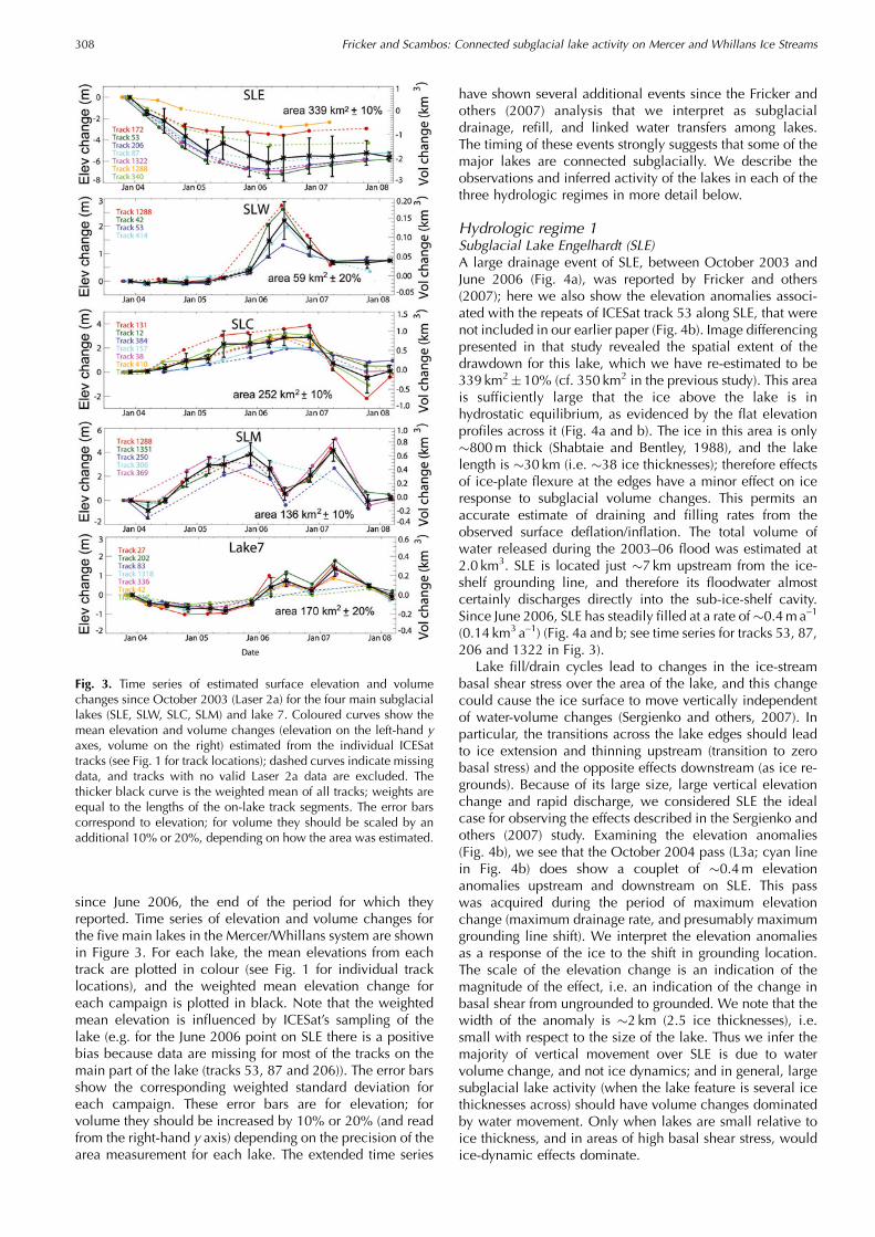
since June 2006, the end of the period for which theyreported. Time series of elevation and volume changes forthe five main lakes in the Mercer/Whillans system are shownin Figure 3. For each lake, the mean elevations from eachtrack are plotted in colour (see Fig. 1 for individual tracklocations), and the weighted mean elevation change foreach campaign is plotted in black. Note that the weightedmean elevation is influenced by ICESat’s sampling of thelake (e.g. for the June 2006 point on SLE there is a positivebias because data are missing for most of the tracks on themain part of the lake (tracks 53, 87 and 206)). The error barsshow the corresponding weighted standard deviation foreach campaign. These error bars are for elevation; forvolume they should be increased by 10% or 20% (and readfrom the right-hand y axis) depending on the precision of thearea measurement for each lake. The extended time series

have shown several additional events since the Fricker andothers (2007) analysis that we interpret as subglacialdrainage, refill, and linked water transfers among lakes.The timing of these events strongly suggests that some of themajor lakes are connected subglacially. We describe theobservations and inferred activity of the lakes in each of thethree hydrologic regimes in more detail below.

Hydrologic regime 1Subglacial Lake Engelhardt (SLE)A large drainage event of SLE, between October 2003 andJune 2006 (Fig. 4a), was reported by Fricker and others(2007); here we also show the elevation anomalies associ-ated with the repeats of ICESat track 53 along SLE, that werenot included in our earlier paper (Fig. 4b). Image differencingpresented in that study revealed the spatial extent of thedrawdown for this lake, which we have re-estimated to be339 km2�10% (cf. 350 km2 in the previous study). This areais sufficiently large that the ice above the lake is inhydrostatic equilibrium, as evidenced by the flat elevationprofiles across it (Fig. 4a and b). The ice in this area is only�800m thick (Shabtaie and Bentley, 1988), and the lakelength is �30 km (i.e. �38 ice thicknesses); therefore effectsof ice-plate flexure at the edges have a minor effect on iceresponse to subglacial volume changes. This permits anaccurate estimate of draining and filling rates from theobserved surface deflation/inflation. The total volume ofwater released during the 2003–06 flood was estimated at2.0 km3. SLE is located just �7 km upstream from the ice-shelf grounding line, and therefore its floodwater almostcertainly discharges directly into the sub-ice-shelf cavity.Since June 2006, SLE has steadily filled at a rate of�0.4ma–1

(0.14 km3 a–1) (Fig. 4a and b; see time series for tracks 53, 87,206 and 1322 in Fig. 3).

Lake fill/drain cycles lead to changes in the ice-streambasal shear stress over the area of the lake, and this changecould cause the ice surface to move vertically independentof water-volume changes (Sergienko and others, 2007). Inparticular, the transitions across the lake edges should leadto ice extension and thinning upstream (transition to zerobasal stress) and the opposite effects downstream (as ice re-grounds). Because of its large size, large vertical elevationchange and rapid discharge, we considered SLE the idealcase for observing the effects described in the Sergienko andothers (2007) study. Examining the elevation anomalies(Fig. 4b), we see that the October 2004 pass (L3a; cyan linein Fig. 4b) does show a couplet of �0.4m elevationanomalies upstream and downstream on SLE. This passwas acquired during the period of maximum elevationchange (maximum drainage rate, and presumably maximumgrounding line shift). We interpret the elevation anomaliesas a response of the ice to the shift in grounding location.The scale of the elevation change is an indication of themagnitude of the effect, i.e. an indication of the change inbasal shear from ungrounded to grounded. We note that thewidth of the anomaly is �2 km (2.5 ice thicknesses), i.e.small with respect to the size of the lake. Thus we infer themajority of vertical movement over SLE is due to watervolume change, and not ice dynamics; and in general, largesubglacial lake activity (when the lake feature is several icethicknesses across) should have volume changes dominatedby water movement. Only when lakes are small relative toice thickness, and in areas of high basal shear stress, wouldice-dynamic effects dominate.

Fig. 3. Time series of estimated surface elevation and volumechanges since October 2003 (Laser 2a) for the four main subglaciallakes (SLE, SLW, SLC, SLM) and lake 7. Coloured curves show themean elevation and volume changes (elevation on the left-hand yaxes, volume on the right) estimated from the individual ICESattracks (see Fig. 1 for track locations); dashed curves indicate missingdata, and tracks with no valid Laser 2a data are excluded. Thethicker black curve is the weighted mean of all tracks; weights areequal to the lengths of the on-lake track segments. The error barscorrespond to elevation; for volume they should be scaled by anadditional 10% or 20%, depending on how the area was estimated.


To aid understanding of SLE, we have produced a lineschematic, along a profile through the lake and overlyingice, using ICESat surface elevation, ice thickness inter-polated from our ice-thickness map (Shabtaie and Bentley,1988), and hydrostatic potential interpolated from thedistribution presented in Figure 2 (Fig. 4c). ICESat track425 crosses SLE almost exactly along-flow, and is nearlycentered on the narrow zone downstream where the outletchannel for the lake is suspected. Because this track wasacquired within hours of the end of a 33 day campaign (andthe campaign terminations vary by a few hours) it has onlybeen acquired twice, during Laser 2c and 3a (Fig. 1 for tracklocation). The SLE schematic (Fig. 4c) shows its location withrespect to the grounding line. The average hydrostaticpressure for SLE is �64 kPa and at the seal it is �128 kPa(relative to the potential pressure at the adjacent groundingline). The steady migration of Engelhardt Ice Ridge reportedby Fricker and others (2007) has continued and is visible inthe ICESat data (Fig. 4b near 83.58 S). It remains an openquestion whether the grounding line in this region ismigrating because of the lake, or whether the groundingline triggered retreat lake drainage.

Hydrologic regime 2Subglacial Lake Whillans (SLW)Fricker and others (2007) inferred from ice surface elevationchange that SLW had just filled in June 2006, after at least2.5 years of inactivity. The additional data since June 2006show that the maximum ice surface elevation over the lakewas in June 2006 (Laser 3f) and was followed by a decreaseof surface elevation over the next two ICESat campaigns(Laser 3g and 3h; Fig. 5a and b). This suggests that theresidence time for the additional water was short(�7months). After that time, the ice surface elevation abovethe lake was about 0.5m above the value it had maintainedfor more than 2 years preceding the filling event (October2003 to November 2005). We estimate the total lake areafrom the MOA image combined with the limits from ICESatelevation anomalies to be 59 km2�20%. The total esti-mated volumes of water SLW received during the fillingevent, and lost during the subsequent drainage event, are�0.13 and �0.09 km3 respectively.

Lake 10Lake 10 is �35 km downstream of SLW and is approximatelydown-gradient (i.e. along a water flowline) in hydrostaticpressure. The surface elevation at this lake has continuallyrisen throughout the ICESat period (Fig. 5b and c). The areaof lake 10 is difficult to establish, but from the MOAcombined with the limits of the ICESat elevation anomalieswe estimate its area to be �25 km2 (�20%). There is anincrease in surface elevation after the SLW drainage event,but this appears to be at nearly the same rate as prior to thatevent. Given the small volumes associated with lake 10, it isdifficult to tell conclusively whether it is linked to SLW.

Ice raft ‘a’Immediately downstream of lake 10 is ice raft ‘a’ (Shabtaieand Bentley, 1987a,b; Alley, 1993; Fig. 1), a region of thickerice moving at the local rate of ice flow. Flow stripingsurrounding ice raft ‘a’ implies that at least at one stage itwas stationary, and the surrounding ice flowed around it.The feature has recently been proposed as a source foricequakes observed in seismograms and the stick–slip

nucleating point for a complex subglacial response to tidalforcing over a large region of the Whillans–Mercer ice plain(Wiens and others, 2008).

Across the downstream face of ice raft ‘a’, the ICESatrepeats for track 83 (Fig. 5c; see Fig. 1 for location) show an

Fig. 4. Hydrologic regime 1. (a) Repeat ICESat elevation profilesalong track 53, which crosses SLE and the grounding zonedownstream, showing: (i) lake drainage from October 2003 throughJune 2006 (Fricker and others, 2007) followed by filling throughMarch 2008; and (ii) retreat of the grounding zone. The pass for3 March 2006 (Laser 3e) that was shown in Fricker and others (2007)has been omitted since the data across the grounding zone areinvalid. (b) Elevation anomalies for track 53 repeats (not previouslypublished). The anomaly plot reveals a flexure portion at the lakeedges (similar to an ice-shelf grounding zone; Padman and Fricker,2006) and flat portion in the centre. Vertical lines correspond to thelimits of the elevation anomaly used to calculate the averageelevation for each track at each campaign epoch. (c) Schematiccross-section through SLE with surface elevation from ICESat track425 and bottom topography from our ice-thickness map (derivedfrom Shabtaie and Bentley, 1988). Vertical exaggeration is four timesgreater for the surface than for the base. The base is colour-coded byhydrostatic pressure from the hydrostatic-potential map in Figure 2.


elevation pattern consistent with an upstream migration ofthe bump, much like the grounding line retreat we observedat Engelhardt Ice Ridge (Fig. 4a). A similar signal (migrationof the bump upstream) is also present on two tracks thatintersect track 83 at ice raft ‘a’ (tracks 191 and 310; seeFig. 1 for location). Additionally, the ICESat repeats acrossthe surface bump associated with ice raft ‘a’ fall into two setsof curves, whose peaks are aligned at two locations, andthere is a jump in the peak location upstream, from one peaklocation to the other, at the same time as the arrival of theSLW water at lake 10, followed by steady continuousmigration upstream (Laser 3g to Laser 3i to Laser 3j), i.e.constant upstream migration of bump, but punctuated withfaster migration coinciding with arrival of water in the lake.This suggests that the lake filling affects the ice dynamics.There is also some evidence of a dipole in the differenceplots, similar to that shown by Sergienko and others (2007).It is possible that we are observing stick–slip motion(Bindschadler and others, 2003), but aliased by the ICESattemporal sampling. Whatever the cause, it seems to be thecase that ice raft ‘a’ has a complex interaction with the ice-stream bed, possibly moderated by subglacial water flow.

Lake 12Lake 12 is the most downstream lake in regime 2 (Figs 1 and2), and its drainage event was documented by Fricker andothers (2007). An elevation decrease of approximately 1.5mwas observed on both ICESat tracks between November2003 and March 2006. From MOA combined with ICESatelevation anomaly limits on two intersecting tracks, weestimate its area to be 64 km2 (�20%). The volume of waterlost by the drainage event was �0.08 km3; the lake filled by�80% of that volume amount soon after SLW drained(Fig. 5b). It appears that floodwater from SLW goes primarilyto lake 12, with some possibly also going to lake 10.

Hydrologic regime 3Subglacial Lake Conway (SLC)The ice surface elevation across SLC started to decreasesometime between June 2006 (L3f) and November 2006(L3g), which we interpret as a flooding event (Fig. 6a). Newimage-differencing results over the region surrounding SLC(2007–05; Fig. 6b) confirm that the lake subsided over thattime period and provide the spatial extent of the subsidencearea; from this image we estimate the SLC area to be252 km2 (�10%). The magnitude of subsidence variedacross the lake, with the largest elevation anomaliesoccurring in the south. This was a significant flooding eventinvolving a large amount of water (�0.83 km3) that persisteduntil November 2007.

Upper lobe of SLCThe hydrostatic-potential map (Fig. 2) revealed a hydrologi-cally flat region �10 km upstream of SLC. The hydrostaticpotential pressure of this upper region is approximately200 kPa greater than that of the center of SLC. ICESat tracks inthe area provide evidence of an active lake, which appears tobe draining with a maximum surface elevation decrease of�2–3m over the period 2003–08 (Fig. 6c). ICESat data overthis lake are noisy due to intense surface crevassing, whichmakes estimates of timing and volume difficult, but theelevation decrease there appears to have started severalmonths prior to SLC, albeit at a much smaller amplitude. Weconsider this an ‘upper lobe’ of SLC, and hereafter refer to it as

Fig. 5. Hydrologic regime 2. (a) Repeat ICESat elevation profiles(upper plot) and elevation anomalies (bottom plot) for track 42across SLW (see Fig. 1 for location). Vertical lines correspond to thelimits of the elevation anomaly used to calculate the averageelevation for each track at each campaign epoch. (b) Time series ofestimated volume changes since October 2003 (Laser 2a) for SLWand lakes 10 and 12; dashed curves indicate data gaps. (c) RepeatICESat elevation profiles for track 83 across lake 10 (see Fig. 1 forlocation).


Fig. 6. Hydrologic regime 3. (a) Repeat ICESat elevation profiles (upper plot) and elevation anomalies (bottom plot) for track 131 across SLC(see Fig. 1 for location). Vertical lines correspond to the limits of the elevation anomaly used to calculate the average elevation for each trackat each campaign epoch. (b) Difference image for the period November 2007–November 2005 over the three lakes. ICESat track segmentsare colour-coded by the elevation decrease over approximately the same period. (c) Repeat ICESat elevation profiles (upper plot) andelevation anomalies (bottom plot) for track 8 across USLC (see Fig. 1 for location). (d) Repeat ICESat elevation profiles (upper plot) andelevation anomalies (bottom plot) for track 1351 across SLM (see Fig. 1 for location). (e) Hydrostatic potential along a line spanning the threelakes (see white dashed line in (b) for location). (f) Time series of estimated volume changes since October 2003 (Laser 2a) for USLC, SLC andSLM; vertical dashed lines show the epochs used for the image difference in (b).


USLC. It seems likely that the drainage of SLCwas triggered inpart by the receipt of floodwater fromUSLC. Since the surfacedeformation of USLC is indiscernible in the difference image(Fig. 6b), we estimate its surface area (177 km2�20%) fromthe limits of the elevation-change signal observed on sevenICESat tracks and co-located surface features in MOA. Theestimated volume of water expelled during theUSLC floodingevent is �0.34 km3 (0.24 km3 between June 2006 andNovember 2007), giving a total of 1.07 km3 for the combinedUSLC/SLC flooding event.

Subglacial Lake Mercer (SLM)The surface elevation of SLM increased steadily fromOctober 2003 until November 2005 (Laser 3d), thendecreased steadily until June 2006 (Laser 3f), which hasbeen interpreted as a drainage event (Fricker and others,2007; Fig. 6d). Track 116 does not have data in eitherFigure 1 or Figure 6b because of large deviations from thereference track, including off-pointing in November 2005.From the difference image (Fig. 6b) we re-estimate the areaof SLM to be 136 km2�10% (cf. 120 km2 by Fricker andothers (2007) based solely on MOA). The total amount ofwater lost by the flooding event was �0.45 km3. After June2006, the elevation increased until February 2007; after thatit decreased again. We interpret this as a secondary drainageevent for SLM, discharging �0.58 km3, and believe it to berelated to the drainage of SLC upstream.

USLC/SLC/SLM linkThe ICESat-derived surface displacements are consistentwith water movement occurring between USLC, SLC andSLM, suggesting that they are connected. A profile takenfrom the new hydrostatic-potential map along the USLC,through SLC and then through SLM shows the pressuregradient among the lakes along a line of minimum hydro-static potential connecting the three, i.e. the likely path ofwater flow between them (Fig. 6e; see Fig. 6b for location).USLC has a hydrostatic potential pressure 230 kPa higherthan SLC, and SLC in turn has �240 kPa higher pressure thanSLM. All three lakes are located in well-defined hydrostaticpotential minima. We note that the hydrostatic potential (orhydraulic head) is not completely flat on the lakesthemselves, and therefore these lakes would not pass oneof Carter and others’ (2007) criteria for a lake. The surfaceelevation of SLM is 100m, �50m above the surfaceelevation of the grounding line. There is a pressure barrierin between the lakes that is presumably breached when SLCdrains; however, the outlet conduit is too small to beresolved at this scale. Figure 2 suggests that the mostprobable pathway for subglacial water from SLC towards theocean would be through SLM.

The hydrologic link between SLC and SLM is alsoapparent from the time-series plot of volume change ofboth lakes (plus USLC) for 2003–08 (Fig. 6f). From this plot,we infer that the floodwater from SLC is directed to SLM: inthe time that SLC lost �0.5 km3 of water (i.e. between June2006 and March 2007), SLM gained �0.45 km3. The lakevolume threshold (i.e. the full capacity of the lake just beforeit drains) appears to be about �0.5 km3 greater than itsvolume immediately after flooding. At around the time whenwater from SLC started to reach SLM (June 2006), SLM hadjust drained. When the capacity of SLM had increased by�0.5 km3 again (March 2007), the lake was full again andstarted to drain. We propose that, once the outlet conduit for

SLM was open, the additional floodwater arriving from SLCmoved directly through SLM (the outlet was hydraulicallyjacked open, i.e. the subglacial water pressure exceeded theice overburden pressure). This is similar to the scenario thatwas recently proposed to have occurred at the AdventureTrench lakes (Carter and others, in press). During thatflooding event, discharge from lake U2 likely passed straightthrough lake U3, since U3 was already full and theadditional water entering it overflowed.

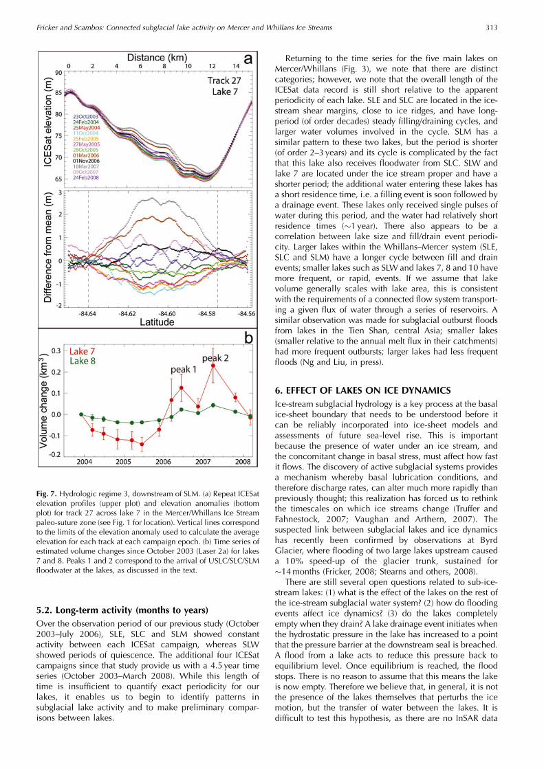
Downstream of SLMThe floodwater from the USLC/SLC/SLM flood appears tohave arrived at two locations down the hydrostatic potentialgradient from SLM (lakes 7 and 8; Fig. 1) at around the sametime (although accurate timing is not possible due to thecoarse temporal sampling of ICESat), and temporarily pondsin these regions. Lake 7 is larger than originally suggested byFricker and others (2007) and appears to be joined to theirlake 9. This inferred large water body is contained within adistinct trough associated with flowband in the Mercer/Whillans Ice Stream suture zone that is clearly visible inMOA. The hydrostatic potential is constant (�28 kPa) alongthis entire elongated feature, and the surface elevation is65–70m; the estimated area from MOA combined withICESat elevation-change limits is �170 km2 (�20%). Repeatelevation profiles for ICESat track 27 across this trough areshown in Figure 7a. Lake 8 is a smaller lake (area from MOAis �52 km2�20%) that sits at a slightly higher hydrostaticpotential (�30 kPa; surface elevation 78m).

Lake 7 appears to have received the majority of thefloodwater, although the residence time for the water therewas short (approximately March–June 2006). It appears thatsome floodwater also went to lake 8, whose activitymatched that of lake 7, i.e. the surface elevations at thislake are in phase with those at lake 7 (Fig. 7b) but at muchlower amplitude. The ICESat tracks across lake 7 that haveno coloured segments in Figure 1 had no valid repeats whenthe lake was full. The timings of the peaks of the time seriesfor lakes 7 and 8 (Fig. 7b) are consistent with these regionsreceiving water from the flooding of SLM (peak 1) and SLC/SLM (peak 2).

5. COMPARISON OF SUBGLACIAL ACTIVITY FORMERCER/WHILLANS LAKES5.1. Short-term activity (days to weeks)In our earlier study (Fricker and others, 2007), we noted thatthe detected elevation-change regions displayed a variety oftemporal signatures, and that changes occur on shorttimescales (e.g. between two ICESat campaigns). We con-sidered whether lake levels might fluctuate on timescalesshorter than the ICESat sampling; if this is the case, our timeseries would be aliased plots of the true lake activity.However, we note that for the larger lakes (see, e.g., the timeseries for SLM; Fig. 3) there are several ICESat tracks acrossthe lake on different days within the 33 day laser campaign.If there was lake activity on the sub-daily or even sub-monthly timescale, we would expect to see variability in thelake states from the different acquisition times of trackswithin the campaigns. Since we do not see this, we believethat the lake states are similar for each pass within the sameICESat campaign, and that it is unlikely that there is anysignificant short-term activity going on within or betweenthese 33 day periods.


5.2. Long-term activity (months to years)Over the observation period of our previous study (October2003–July 2006), SLE, SLC and SLM showed constantactivity between each ICESat campaign, whereas SLWshowed periods of quiescence. The additional four ICESatcampaigns since that study provide us with a 4.5 year timeseries (October 2003–March 2008). While this length oftime is insufficient to quantify exact periodicity for ourlakes, it enables us to begin to identify patterns insubglacial lake activity and to make preliminary compar-isons between lakes.

Returning to the time series for the five main lakes onMercer/Whillans (Fig. 3), we note that there are distinctcategories; however, we note that the overall length of theICESat data record is still short relative to the apparentperiodicity of each lake. SLE and SLC are located in the ice-stream shear margins, close to ice ridges, and have long-period (of order decades) steady filling/draining cycles, andlarger water volumes involved in the cycle. SLM has asimilar pattern to these two lakes, but the period is shorter(of order 2–3 years) and its cycle is complicated by the factthat this lake also receives floodwater from SLC. SLW andlake 7 are located under the ice stream proper and have ashorter period; the additional water entering these lakes hasa short residence time, i.e. a filling event is soon followed bya drainage event. These lakes only received single pulses ofwater during this period, and the water had relatively shortresidence times (�1 year). There also appears to be acorrelation between lake size and fill/drain event periodi-city. Larger lakes within the Whillans–Mercer system (SLE,SLC and SLM) have a longer cycle between fill and drainevents; smaller lakes such as SLW and lakes 7, 8 and 10 havemore frequent, or rapid, events. If we assume that lakevolume generally scales with lake area, this is consistentwith the requirements of a connected flow system transport-ing a given flux of water through a series of reservoirs. Asimilar observation was made for subglacial outburst floodsfrom lakes in the Tien Shan, central Asia; smaller lakes(smaller relative to the annual melt flux in their catchments)had more frequent outbursts; larger lakes had less frequentfloods (Ng and Liu, in press).

6. EFFECT OF LAKES ON ICE DYNAMICSIce-stream subglacial hydrology is a key process at the basalice-sheet boundary that needs to be understood before itcan be reliably incorporated into ice-sheet models andassessments of future sea-level rise. This is importantbecause the presence of water under an ice stream, andthe concomitant change in basal stress, must affect how fastit flows. The discovery of active subglacial systems providesa mechanism whereby basal lubrication conditions, andtherefore discharge rates, can alter much more rapidly thanpreviously thought; this realization has forced us to rethinkthe timescales on which ice streams change (Truffer andFahnestock, 2007; Vaughan and Arthern, 2007). Thesuspected link between subglacial lakes and ice dynamicshas recently been confirmed by observations at ByrdGlacier, where flooding of two large lakes upstream causeda 10% speed-up of the glacier trunk, sustained for�14months (Fricker, 2008; Stearns and others, 2008).

There are still several open questions related to sub-ice-stream lakes: (1) what is the effect of the lakes on the rest ofthe ice-stream subglacial water system? (2) how do floodingevents affect ice dynamics? (3) do the lakes completelyempty when they drain? A lake drainage event initiates whenthe hydrostatic pressure in the lake has increased to a pointthat the pressure barrier at the downstream seal is breached.A flood from a lake acts to reduce this pressure back toequilibrium level. Once equilibrium is reached, the floodstops. There is no reason to assume that this means the lakeis now empty. Therefore we believe that, in general, it is notthe presence of the lakes themselves that perturbs the icemotion, but the transfer of water between the lakes. It isdifficult to test this hypothesis, as there are no InSAR data

Fig. 7. Hydrologic regime 3, downstream of SLM. (a) Repeat ICESatelevation profiles (upper plot) and elevation anomalies (bottomplot) for track 27 across lake 7 in the Mercer/Whillans Ice Streampaleo-suture zone (see Fig. 1 for location). Vertical lines correspondto the limits of the elevation anomaly used to calculate the averageelevation for each track at each campaign epoch. (b) Time series ofestimated volume changes since October 2003 (Laser 2a) for lakes7 and 8. Peaks 1 and 2 correspond to the arrival of USLC/SLC/SLMfloodwater at the lakes, as discussed in the text.


over the lakes coinciding with the ICESat period, and theregion discussed here is too far south for much higher-resolution visible-band image data for velocity mapping. Inthe absence of simultaneous velocity data over the Mercerand Whillans Ice Streams, it is not possible to determinewhether the flooding events documented here affected icevelocities. The link between lakes and ice dynamics is beinginvestigated during ongoing fieldwork in the region duringthe 2007/08 and 2008/09 Antarctic field seasons (Tulaczykand others, 2008). In the future, data from ICESat-II(currently planned for launch in 2015) or other elevationsatellite or airborne missions, combined with coincidentvelocity measurements, would provide much-needed in-formation towards understanding the link between thesubglacial system and ice dynamics.

7. CONCLUSIONSWe have examined the activity of the subglacial watersystem beneath lower Mercer and Whillans Ice Streams forthe period October 2003–March 2008 using ICESat repeat-track analysis and satellite image differencing. Since1 January 2007, the temporal sampling of the ICESat datahas reduced to twice a year, but the most recent data haverevealed important new information about this subglacialwater system. Several significant events took place duringthat time. The most noteworthy event was the drainage ofUSLC/SLC since June 2006, discharging an estimated0.86 km3 of water. ICESat analyses suggest that some ofthis water was directed to SLM; while SLC was draining,SLM filled and then drained, strongly suggesting that thesetwo lakes are connected hydrologically. Water from thisflood was channeled downstream towards the ocean alonga surface depression lying along the suture zone betweenMercer and Whillans Ice Streams, and pooled theretemporarily. The locations of these downstream signalscorrespond to depressions in the surface topography thatare also visible in the MOA image of the region. SLW alsoappears to be linked to the next region down the hydro-static potential gradient in its regime. Our analysis alsolooked at SLW and subglacial activity near ice raft ‘a’(Alley, 1993), a prominent feature of the ice plain ofWhillans Ice Stream. Inferred hydrologic activity, marginalchanges akin to grounding-line retreat, and results of otherstudies showing that the ice raft is a locus of stick–slipactivity over a large portion of the ice plain (Wiens andothers, 2008) all point to this feature having a complexinteraction with the ice-plain bed.

With the 5 year time-span of ICESat data, we are now ableto investigate the activity cycles of the lakes in this system,although the time series is still short relative to the apparentperiodicity of the lakes. We notice distinct patterns in lakeactivity: larger lakes located next to ice-stream shearmargins have long, steady fill/drain cycles; whereas smallerlakes under the faster-flowing parts of the ice stream haveshorter cycles and short residence times for the additionalwater. We believe that the frequency of outburst flood eventsis related to subglacial water supply and lake capacity, butmay involve other factors such as: basal lithology or tillthickness; local bed and ice surface relief (e.g. the variabilityof the hydrostatic potential field); and, as we show here, theactivity of lakes hydrologically upstream of a given sub-glacial reservoir.

ACKNOWLEDGEMENTSWe thank B. Smith, S. O’Neel and R. Radpour for help withthe ICESat data interpretation. We also thank T. Haran forhelp with the MODIS image differencing and hydrostatic-potential mapping, and S. Carter for providing his SLMoutline. We thank NASA’s ICESat Science Project fordistribution of the ICESat data (see http://icesat.gsfc.nasa.govand http://nsidc.org/data/icesat). We thank R. Bingham,N. Glasser and an anonymous reviewer for thoroughreviewing, which greatly improved the paper. H.A.F. wassupported by NASA grant NNX07AL18G.

REFERENCESAlley, R.B. 1993. In search of ice-stream sticky spots. J. Glaciol.,

39(133), 447–454.Bell, R.E., M. Studinger, C.A. Shuman, M.A. Fahnestock and

I. Joughin. 2007. Large subglacial lakes in East Antarcticaat the onset of fast-flowing ice streams. Nature, 445(7130),904–907.

Bindschadler, R.A. and P.L. Vornberger. 1994. Detailed elevationmap of Ice Stream C, Antarctica, using satellite imagery andairborne radar. Ann. Glaciol., 20, 327–335.

Bindschadler, R.A., M.A. King, R.B. Alley, S. Anandakrishnan andL. Padman. 2003. Tidally controlled stick–slip discharge of aWest Antarctic ice stream. Science, 301(5636), 1087–1089.

Carter, S.P., D.D. Blankenship, M.F. Peters, D.A. Young, J.W. Holtand D.L. Morse. 2007. Radar-based subglacial lake classificationin Antarctica. Geochem. Geophys. Geosyst., 8(3), Q03016.(10.1029/2006GC001408.)

Carter, S.P., D.D. Blankenship, D.A. Young, M.E. Peters, J.W. Holtand M.J. Siegert. In press. Dynamic distributed drainage impliedby the flow evolution of the 1996–1998 Adventure Trenchsubglacial outburst flood. Earth Planet. Sci. Lett.

Engelhardt, H., N. Humphrey, B. Kamb and M. Fahnestock. 1990.Physical conditions at the base of a fast moving Antarctic icestream. Science, 248(4951), 57–59.

Fricker, H.A. 2008. Glaciology: water slide. Nature Geosci., 1(12),809–816.

Fricker, H.A. and L. Padman. 2006. Ice shelf grounding zonestructure from ICESat laser altimetry. Geophys. Res. Lett., 33(15),L15502. (10.1029/2006GL026907.)

Fricker, H.A., A. Borsa, B. Minster, C. Carabajal, K. Quinn andB. Bills. 2005. Assessment of ICESat performance at the salar deUyuni, Bolivia. Geophys. Res. Lett., 32(21), L21S06 (10.1029/2005GL023423.)

Fricker, H.A., T. Scambos, R. Bindschadler and L. Padman. 2007.An active subglacial water system in West Antarctica mappedfrom space. Science, 315(5818), 1544–1548.

Goodwin, I.D. 1988. The nature and origin of a jokulhlaup nearCasey Station, Antarctica. J. Glaciol., 34(116), 95–101.

Gray, L., I. Joughin, S. Tulaczyk, V.B. Spikes, R. Bindschadler andK. Jezek. 2005. Evidence for subglacial water transport in theWest Antarctic Ice Sheet through three-dimensional satelliteradar interferometry. Geophys. Res. Lett., 32(3), L03501.(10.1029/2004GL021387.)

Haran, T.M., M.A. Fahnestock and T.A. Scambos. 2002. De-stripingof MODIS optical bands for ice sheet mapping andtopography. [Abstract C12A-1003.] Eos, 88(47), Fall Meet.Suppl., 317.

Haran, T.M., T.A. Scambos, M.A. Fahnestock, D. Yi and H.J. Zwally.2006. A digital elevation model of west Antarctica from MODISand ICESat: method, accuracy, and applications. [AbstractC21A-1131.] Eos, 87(52), Fall Meet. Suppl.

Iken, A. and R.A. Bindschadler. 1986. Combined measurements ofsubglacial water pressure and surface velocity of Findelen-gletscher, Switzerland: conclusions about drainage system andsliding mechanism. J. Glaciol., 32(110), 101–119.


Joughin, I.R., S. Tulaczyk and H.F. Engelhardt. 2003. Basal meltbeneath Whillans Ice Stream and Ice Streams A and C, WestAntarctica. Ann. Glaciol., 36, 257–262.

Kamb, B. 2001. Basal zone of the West Antarctic ice streams and itsrole in lubrication of their rapid motion. In Alley, R.B. andR.A. Bindschadler, eds. The West Antarctic ice sheet: behaviorand environment. Washington, DC, American GeophysicalUnion, 157–199. (Antarctic Research Series 77.)

Ng, F. and S. Liu. In press. Temporal dynamics of a jokulhlaupsystem. J. Glaciol., 55(191).

Robin, G.de Q., C.W.M. Swithinbank and B.M.E. Smith. 1970.Radio echo exploration of the Antarctic ice sheet. IASH Publ. 86(Symposium at Hanover 1968 – Antarctic GlaciologicalExploration (ISAGE)), 97–115.

Scambos, T.A. and M.A. Fahnestock. 1998. Improving digitalelevation models over ice sheets using AVHRR-based photo-clinometry. J. Glaciol., 44(146), 97–103.

Scambos, T.A., T.M. Haran, M.A. Fahnestock, T.H. Painter andJ. Bohlander. 2007. MODIS-based Mosaic of Antarctica (MOA)data sets: continent-wide surface morphology and snow grainsize. Remote Sens. Environ., 111(2–3), 242–257.

Sergienko, O.V., D.R. MacAyeal and R.A. Bindschadler. 2007.Causes of sudden, short-term changes in ice-stream surfaceelevation. Geophys. Res. Lett., 34(22), L22503. (10.1029/2007GL031775.)

Shabtaie, S. and C.R. Bentley. 1987a. Correction to ‘West Antarcticice streams draining into the Ross Ice Shelf: configuration andmass balance’. J. Geophys. Res., 92(B9), 9451.

Shabtaie, S. and C.R. Bentley. 1987b. West Antarctic ice streamsdraining into the Ross Ice Shelf: configuration and mass balance.J. Geophys. Res., 92(B2), 1311–1336.

Shabtaie, S. and C.R. Bentley. 1988. Ice-thickness map of the WestAntarctic ice streams by radar sounding. Ann. Glaciol., 11,126–136.

Shreve, R.L. 1972. Movement of water in glaciers. J. Glaciol.,11(62), 205–214.

Shuman, C.A. and 6 others. 2006. ICESat Antarctic elevation data:preliminary precision and accuracy assessment. Geophys. Res.Lett., 33(7), L07501. (10.1029/2005GL025227.)

Siegert, M.J. and J.L. Bamber. 2000. Correspondence. Subglacialwater at the heads of Antarctic ice-stream tributaries. J. Glaciol.,46(155), 702–703.

Siegert, M.J., S. Carter, I. Tabacco, S. Popov and D.D. Blankenship.2005. A revised inventory of Antarctic subglacial lakes. Antarct.Sci., 17(3), 453–460.

Spikes, V.B., B.M. Csatho, G.S. Hamilton and I.M. Whillans. 2003.Thickness changes on Whillans Ice Stream and Ice Stream C,West Antarctica, derived from laser altimeter measurements.J. Glaciol., 49(165), 223–230.

Stearns, L.A., B.E. Smith and G.S. Hamilton. 2008. Increased flowspeed on a large East Antarctic outlet glacier caused bysubglacial floods. Nature Geosci., 1(12), 827–831.

Sun, X., J.B. Abshire and D. Yi. 2003. Geoscience laser altimetersystem (GLAS) – characteristics and performance of the altimeterreceiver. [Abstr. C32A-0432.] Eos, 84(46), Fall Meet. Suppl.

Truffer, M. and M. Fahnestock. 2007. Climate change: rethinkingice sheet time scales. Science, 315(5818), 1508–1510.

Tulaczyk, S., R. Pettersson, N. Quintana-Krupinski, H. Fricker,I. Joughin and B. Smith. 2008. Do dynamic subglacial lakesimpact temporal behavior of fast-flowing ice streams? GPS andradar investigations on twoWest Antarctic ice streams. Geophys.Res. Abstr. 10, 11565. (1607-7962/gra/EGU2008-A-11565.)

Vaughan, D.G. and R. Arthern. 2007. Climate change: why is ithard to predict the future of ice sheets? Science, 315(5818),1503–1504.

Wiens, D.A., S. Anandakrishnan, J.P. Wineberry and M.A. King.2008. Simultaneous teleseismic and geodetic observations of thestick–slip motion of an Antarctic ice stream. Nature, 453(7196),770–774.

Wingham, D.J., M.J. Siegert, A. Shepherd and A.S. Muir. 2006.Rapid discharge connects Antarctic subglacial lakes. Nature,440(7087), 1033–1036.

MS received 3 September 2008 and accepted in revised form 8 December 2008


connected subglacial lake activity on lower mercer and

Documents