conjugate heat transfer model of a film cooled flat plate · a print of the flat plate showing the...
TRANSCRIPT
CONJUGATE HEAT TRANSFER MODEL OF A FILM COOLED
FLAT PLATE
Undergraduate Honors Thesis
Presented in Partial Fulfillment of the Requirements for Graduation with Honors
Research Distinction in the Department of Mechanical Engineering at The Ohio State
University
By
Kyle James Sherman
****
The Ohio State University
2015
Thesis Examination Committee:
Professor Randall Mathison, Advisor
Professor Michael Dunn

Copyright by
Kyle J. Sherman
2015

ii
ABSTRACT
Turbine blades are used in a variety of applications and are often subject to
extreme temperatures. It is imperative that these conditions are taken into consideration
during the design process in order to maximize life. In many turbines, cooling holes are
strategically placed along the blades, allowing coolant to seep through and preventing
concentrations of heat flux. Experiments have been conducted at the Gas Turbine
Laboratory (GTL) in the past to measure the heat transfer distribution over the surface of
a film-cooled flat plate that represents a simplified turbine blade. Computational fluid
dynamics (CFD) models were created to predict the heat transfer distribution, but there
was a large margin of error between the CFD model and experimental results.
The previous CFD models of the flat plate only took fluid convection into
consideration. This study produced and analyzed a conjugate heat transfer model of the
flat plate, which incorporates solid conduction in addition to fluid convection. The model
was able to more accurately predict the heat transfer trends across the flat plate in some
cases, but further work is necessary to obtain closer agreement between the predictions
and experimental data. Validated computational models can be very useful in determining
where additional cooling holes on turbine blades may be necessary. Continuing to
improve the accuracy of predictions for this flat plate will demonstrate new modeling
techniques that can be applied in the turbine design process to develop gas turbine
engines with increased efficiency and reliability.

iii
ACKNOWLEDGEMENTS
I would like to thank my faculty advisor, Dr. Randall Mathison, for all of his
guidance and support as I navigated through the challenges of this study. You were
always helpful in answering any questions that arose and continually fueled my
progression.
I would also like to thank PhD student Jeremy Nickol, who provided a basis for
this study with his Master’s Thesis. This project would not have been possible without
your previous work and extensive assistance in the lab.
Finally, I sincerely appreciate the sponsorship of both the NASA Ohio Space
Grant Consortium as well as The Ohio State University College of Engineering in my
endeavors.
iv
VITA
1992………………………… Born – Seattle, Washington
2011 – Present……………… B.S. Mechanical Engineering, The Ohio State University
FIELDS OF STUDY
Major Field: Mechanical Engineering
v
TABLE OF CONTENTS
ABSTRACT ........................................................................................................................ ii
ACKNOWLEDGEMENTS ............................................................................................... iii
VITA .................................................................................................................................. iv
LIST OF FIGURES ........................................................................................................... vi
LIST OF TABLES ............................................................................................................ vii
NOMENCLATURE AND ABBREVIATIONS .............................................................. viii
INTRODUCTION .............................................................................................................. 1
1.1 Background Information ........................................................................................ 1
1.2 Research Purpose and Objectives .......................................................................... 2
EXPERIMENTAL SETUP ................................................................................................. 3
2.1 Small Calibration Facility ...................................................................................... 3
COMPUTATIONAL FLUID DYNAMICS SETUP .......................................................... 6
3.1 Geometry and Domain Creation ............................................................................ 6
3.2 Meshing .................................................................................................................. 8
3.3 Input Parameters .................................................................................................. 12
RESULTS AND DISCUSSION ....................................................................................... 15
4.1 Steady State Simulations ...................................................................................... 15
4.2 Transient Simulations .......................................................................................... 20
CONCLUSION ................................................................................................................. 23
5.1 Final Statements ................................................................................................... 23
5.2 Future Work ......................................................................................................... 23
REFERENCES ................................................................................................................. 25

vi
LIST OF FIGURES
FIGURE 1: SCHEMATIC OF THE SCF [1] ................................................................................................... 3
FIGURE 2: PHOTOGRAPH OF THE SCF [1] ............................................................................................... 4
FIGURE 3: PHOTOGRAPH OF THE FLAT PLATE [1] ............................................................................... 5
FIGURE 4: PRINT OF FLAT PLATE AND HOLE PATTERN – UNITS IN INCHES [1] .......................... 6
FIGURE 5: FIRST THREE COOLING HOLE ROWS MESHED IN FLUID DOMAIN ............................ 10
FIGURE 6: COOLING HOLE INLET IN FLUID DOMAIN ....................................................................... 10
FIGURE 7: FINAL MESH OF SOLID AND FLUID DOMAINS ............................................................... 12
FIGURE 8: DIAGRAM OF TEST SECTION [1] ......................................................................................... 12
FIGURE 9: NICKOL’S NCHFR DATA AND PREDICTION [1] ............................................................... 16
FIGURE 10: NCHFR DATA AND STEADY STATE CONJUGATE MODEL PREDICTION ................. 17
FIGURE 11: HEAT FLUX DISTRIBUTION FOR M=0.3 AT STEADY STATE – UNITS IN W/M2 ...... 18
FIGURE 12: HEAT FLUX DISTRIBUTION FOR M=1.5 AT STEADY STATE – UNITS IN W/M2 ...... 18
FIGURE 13: TEMPERATURE DISTRIBUTION FOR M=0.3 AT STEADY STATE – UNITS IN K ...... 19
FIGURE 14: NCHFR DATA AND CONJUGATE MODEL PREDICTIONS AT M=0.3 .......................... 21
FIGURE 15: NCHFR DATA AND CONJUGATE MODEL PREDICTIONS AT M=1.5 .......................... 22
vii
LIST OF TABLES
TABLE 1: COOLING HOLE ROW INFORMATION [1] ............................................................................. 7
TABLE 2: MAIN INLET AND OUTLET BOUNDARY CONDITIONS ................................................... 14
TABLE 3: COOLING HOLE INLET BOUNDARY CONDITIONS ........................................................... 14
TABLE 4: INITIAL CONDITIONS .............................................................................................................. 14
viii
NOMENCLATURE AND ABBREVIATIONS
NOMENCLATURE
A Area
D Diameter
M Blowing Ratio
𝑚 Mass Flow Rate
NCHFR Non-Corrected Heat Flux Reduction
~Nu Modified Nusselt Number
Nu Actual Nusselt Number
P Pressure
q’’ Heat Flux
T Temperature
V Velocity
xBLB Distance Downstream from Boundary Layer Bleed
x/D Normalized Distance Downstream
ABBREVIATIONS
BLB Boundary Layer Bleed
CFD Computational Fluid Dynamics
FAV Fast-Acting Valve
GTL Gas Turbine Laboratory

ix
OSU The Ohio State University
SCF Small Calibration Facility
1
Chapter 1 INTRODUCTION
1.1 Background Information
Gas turbines have been the backbone of power generation for decades, and more
recently the foundation for large aircraft propulsion. As turbine engine manufacturers
continue to strive for increasing efficiencies, higher operating temperatures are required.
It is critical for turbine blades to be designed in such a way to avoid thermal failure.
Cooling holes are often placed along the blades at strategic locations to create a film of
cooled air over the surface of the blade. These technologies allow turbine blades to
operate at higher inlet temperatures while ensuring their reliability and lifespan. In order
to determine the most effective positions to place cooling holes, the heat flux at different
locations along the blade must be known.
Experiments are necessary to measure the heat flux distribution for different
turbine blade geometries with various cooling hole patterns. Rotating experiments are one
way to investigate turbine behaviors, but these are complex and relatively difficult to set
up. Experiments can also be performed on flat plates, which simplify flow over the high-
pressure surface of a turbine blade. This study focuses on a specific flat plate experiment
performed at the GTL, most recently studied by Jeremy Nickol as part of his Master’s
Thesis [1].
2
1.2 Research Purpose and Objectives
The flat plate experiment was originally designed and instrumented by Simone
Bernasconi [2]. Shanon Davis collected an extensive amount of data on the experiment,
but her analysis was limited [3]. Nickol performed additional experiments to more
accurately determine the coolant mass flow rates and thoroughly analyzed the data Davis
collected [1]. He also developed a CFD model of experiment and compared the
simulation results to the experimental data. The model showed some agreement in heat
flux trends, but the absolute heat flux values exhibited significant deviation from
experimental data.
The purpose of this research was to establish best practices for computational flat
plate models by improving the accuracy of heat flux predictions of the flat plate. CFD
models that can be successfully validated by experimental data are extremely valuable, as
they can easily be adjusted to confidently investigate the effects of different cooling hole
geometries. Hence, an accurate computational model can be much more time-efficient
and cost-efficient than conducting several experiments.

3
Chapter 2 EXPERIMENTAL SETUP
2.1 Small Calibration Facility
As previously noted, this research produced computational models of a flat plate
experiment in the Small Calibration Facility (SCF) at The Ohio State University (OSU)
GTL. Originally constructed to calibrate instruments for larger experiments, the SCF
consists of a medium-duration blowdown tunnel and is also used as a test facility for
smaller experiments such as the relevant flat plate experiment [1]. A schematic and
photograph of the SCF setup for the flat plate experiment are shown below in Figure 1
and Figure 2 respectively.
Figure 1: Schematic of the SCF [1]
4
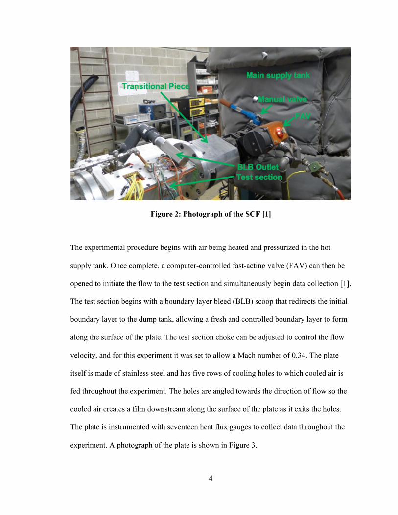
Figure 2: Photograph of the SCF [1]
The experimental procedure begins with air being heated and pressurized in the hot
supply tank. Once complete, a computer-controlled fast-acting valve (FAV) can then be
opened to initiate the flow to the test section and simultaneously begin data collection [1].
The test section begins with a boundary layer bleed (BLB) scoop that redirects the initial
boundary layer to the dump tank, allowing a fresh and controlled boundary layer to form
along the surface of the plate. The test section choke can be adjusted to control the flow
velocity, and for this experiment it was set to allow a Mach number of 0.34. The plate
itself is made of stainless steel and has five rows of cooling holes to which cooled air is
fed throughout the experiment. The holes are angled towards the direction of flow so the
cooled air creates a film downstream along the surface of the plate as it exits the holes.
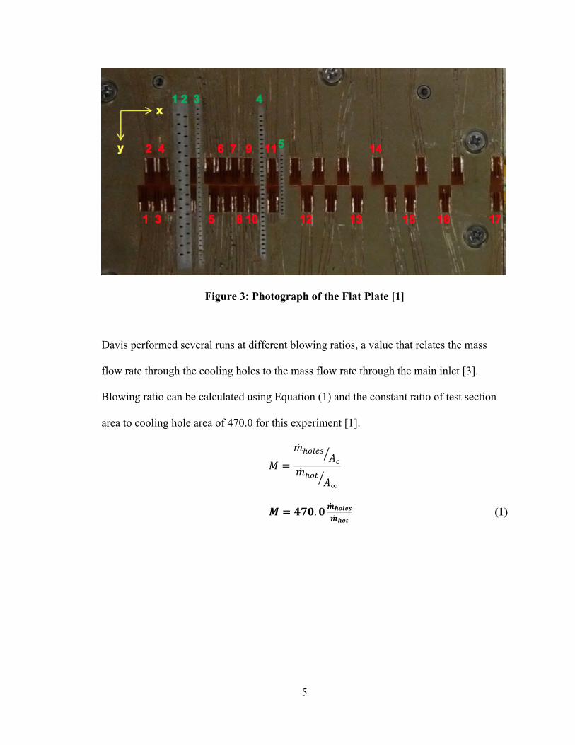
The plate is instrumented with seventeen heat flux gauges to collect data throughout the
experiment. A photograph of the plate is shown in Figure 3.
5
Figure 3: Photograph of the Flat Plate [1]
Davis performed several runs at different blowing ratios, a value that relates the mass
flow rate through the cooling holes to the mass flow rate through the main inlet [3].
Blowing ratio can be calculated using Equation (1) and the constant ratio of test section
area to cooling hole area of 470.0 for this experiment [1].
𝑀 =𝑚!!"#$
𝐴!𝑚!!"
𝐴!
𝑴 = 𝟒𝟕𝟎.𝟎𝒎𝒉𝒐𝒍𝒆𝒔𝒎𝒉𝒐𝒕
(1)
6
Chapter 3 COMPUTATIONAL FLUID DYNAMICS SETUP
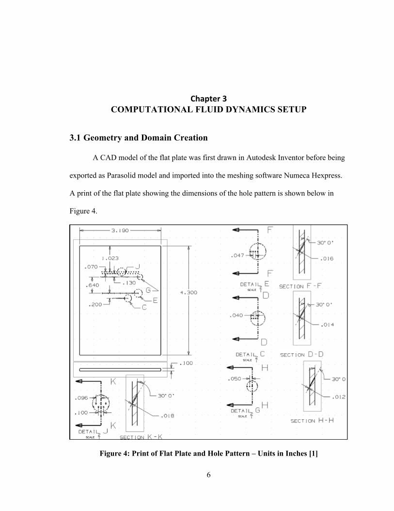
3.1 Geometry and Domain Creation
A CAD model of the flat plate was first drawn in Autodesk Inventor before being
exported as Parasolid model and imported into the meshing software Numeca Hexpress.
A print of the flat plate showing the dimensions of the hole pattern is shown below in
Figure 4.
Figure 4: Print of Flat Plate and Hole Pattern – Units in Inches [1]

7
In order to decrease the mesh size and reduce computation time, the entire width
of the plate was not modeled. This was possible because the experiment only measures
heat flux very close to the center of the plate width. The effect of the cooling holes closer
to the edges of the plate on the heat flux at the center is negligible. In addition, the entire
height of the fluid domain was not modeled, as the flow further away from the plate in
the z-direction has no effect on the behaviors at the surface of the plate.
Details of the cooling hole rows are tabulated below in Table 1. The x-axis is
defined in the direction of flow, and xBLB is denoted as the x-distance from the BLB
scoop to the center of the cooling hole.
Table 1: Cooling Hole Row Information [1]
Row #
No. Holes (Actual)
No. Holes (Modeled)
xBLB Diameter Δy in (mm) in (μm) in (mm)
1 16 4 3.370 85.60 0.018 457 0.096 2.44 2 15 3 3.440 87.38 0.018 457 0.100 2.54 3 32 6 3.570 90.68 0.012 305 0.050 1.27 4 31 7 4.210 106.93 0.016 406 0.047 1.19 5 16 8 4.410 112.01 0.014 356 0.040 1.02
In order to simplify the model, the solid domain only modeled the stainless steel
test section of the flat plate, and the conduction through the stainless steel BLB scoop
was not incorporated. However, the formation of the boundary layer in the fluid domain
is critical to accurately modeling the flow, so the fluid domain was modeled from the
beginning of the boundary layer scoop.
When creating each domain from the geometry, it was discovered that a very
precise triangulation was necessary due to the size and detail of the cooling holes. For
both the fluid and solid domains, the minimum facet lengths were adjusted to 0.1 mm
8
while the curve and surface resolutions were set to a value of 2.0 when creating the
domain triangulation.
3.2 Meshing
All meshing was performed with the Numeca Hexpress software. Hexpress
follows a logical order of five stages when meshing a domain: creation of an initial mesh,
adaptation of the mesh to geometry, snapping to geometry, mesh optimization, and
creation of viscous layers.
The initial mesh stage produces a coarse mesh based on the number of
subdivisions in the direction of each axis as a starting point to be locally refined as
necessary. For the initial mesh of both the solid and fluid domains, the subdivisions of
each axis were set as ratios of their actual dimensions to the nearest whole number so the
cells generated were approximately cubic.
The adapt to geometry stage allows for refinement of the initial mesh wherever
necessary. In the fluid domain, all of the cooling holes passages required significant
refinement. The aim was to have at least 10 cells across the diameter of each cooling hole
after this stage. The surface in contact with the solid domain also required refinement in
the z-direction in order to accurately capture the boundary layer. In the solid domain,
some refinement was used at the surface contacting the fluid, and the cooling hole
surfaces also had to be refined in order to capture the curvature of each hole.
The default settings were used for both the snap to geometry and optimization
stages when meshing both domains. The snap to geometry stage projects cells wherever
there may be voids or overextensions of cells in the geometrical boundaries of the

9
domain. The optimization stage analyzes the mesh and fixes or removes any invalid cells
that may exist.
The viscous layers stage further refines cells near edges where the fluid flow
contacts a solid and boundary layers develop. This stage was unnecessary in the solid
domain, but viscous layers were added in the fluid domain around the edges of the
cooling hole passages as well as at the surface in contact with the solid domain. The
thickness and number of viscous layers were determined based on a Reynolds number
computed within the program from a given reference length and kinematic viscosity. The
air densities through the cooling holes and the main inlet were first calculated based on
the temperature of the air, which were then used to calculate the kinematic viscosities.
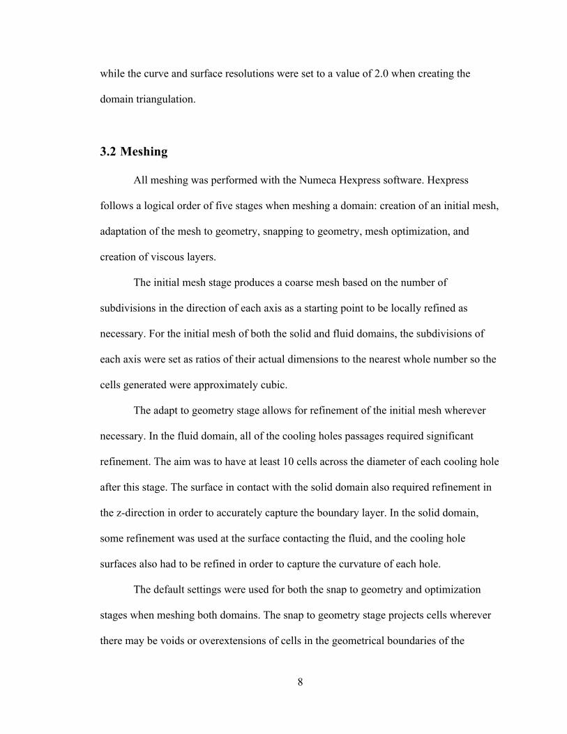
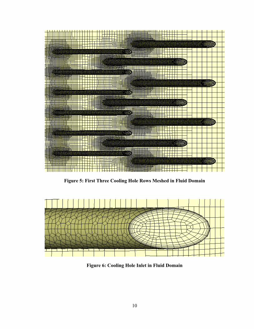
The completed mesh of the first three rows of cooling holes in the fluid domain is shown
in Figure 5. It can clearly be seen that the cooling holes passages required much more
refinement than the surface contacting the solid. Figure 6 shows a close-up view of a
cooling hole inlet in the fluid domain.
10
Figure 5: First Three Cooling Hole Rows Meshed in Fluid Domain
Figure 6: Cooling Hole Inlet in Fluid Domain
11
There are a number of cells that span across the cooling hole internally to allow
the flow to be adequately captured. The viscous layer cells are also visible in the figure,
which begin with the thinnest layer bordering the geometrical boundary and increase in
thickness by a stretching ratio of 1.4 as they progress inward.
The boundary condition type of all faces must be specified within the meshing
software. The mirror boundary condition was set for the two sides of the fluid domain as
well as the surface not contacting the solid domain. This condition assumes the flow on
the inside is mirrored to the outside of the domain, and was used because the fluid
domain is scaled down from the actual experiment and flow does extend beyond those
boundaries. The flow would be altered if those surfaces were set as solid walls. The main
inlet, all cooling hole inlets, and the outlet were also defined in the fluid domain. Lastly,
the software searched for all of the locations where the two domains were in contact and
set each of the contacting pairs as full non-matching connections, allowing them to
interact during simulations. The final mesh contained about 1.8 million cells in the fluid
domain and about 400,000 cells in the solid domain. A side view of the mesh is shown
below in Figure 7. A labeled diagram of the test section with the same orientation is also
shown in Figure 8 for reference.

12
Figure 7: Final Mesh of Solid and Fluid Domains
Figure 8: Diagram of Test Section [1]
3.3 Input Parameters
Numeca FINE/Open was the CFD software used for all computations, which were
executed in serial mode on a computer with 8GB of RAM and a quad-core processor with
clock speeds of 3.40 GHz per core. The computer ran the 64-bit version Windows 7
Professional and FINE/Open version 3.1-3. The multi-block mesh was imported into the
software to prepare and run the simulations. This thesis will analyze four separate
computations run on the mesh. Two different blowing ratios (M=1.5 and M=0.3) were
analyzed with a steady state and a transient simulation at each blowing ratio. These two
13
blowing ratios were chosen because they were the highest and lowest blowing ratios run
experimentally.
Several parameters were consistent across the simulations. The fluid model was
set to air as a real gas, using a Turbulent Navier-Stokes flow model and a Spalart-
Allmaras Turbulence model [4]. The Reynolds Number was calculated for the flow
models based on the length of the fluid domain in the x-direction and the velocity of the
flow. The velocity was calculated based on the known Mach number and the speed of
sound at the respective static temperature of the fluid, which differed by blowing ratio.
The thermal conductivity of the solid model was set as a value greater than the actual
thermal conductivity of stainless steel in order to analyze the effects of the conjugate
model. At first, isothermal conditions were applied to all solid walls other than the
solid/fluid interface. However, the software would not cooperate with these conditions
and they caused the solver to crash after only a couple of iterations every time. The mass
flow rates through the main inlet and cooling hole inlets and as well as the static
temperatures were set based on experimental data and varied by blowing ratio. Due to the
fluid domain being scaled down, the main inlet mass flow rate had to be scaled down by a
ratio of the computational inlet area over the true inlet area so that the inlet mass flux
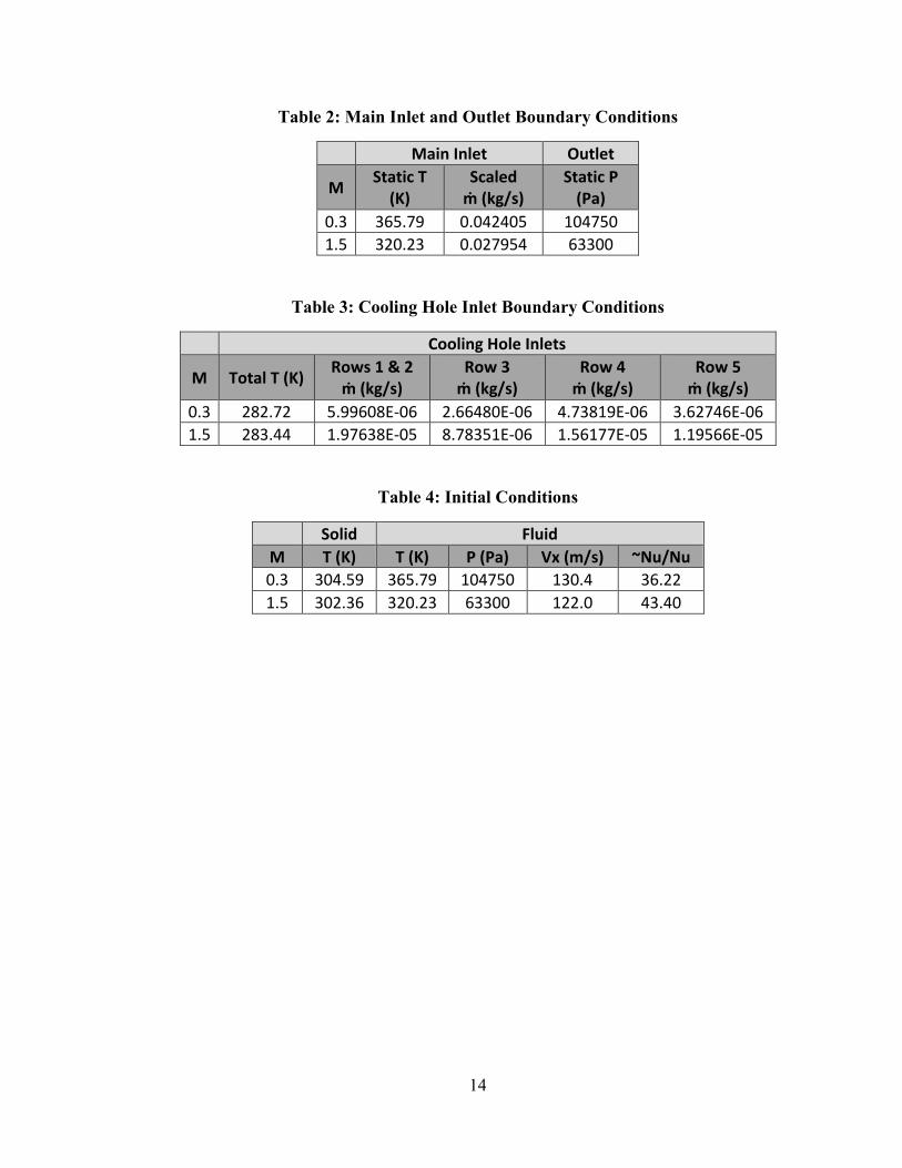
remained constant. The boundary conditions for the main inlet and outlet are shown in
Table 2 and the boundary conditions of the cooling holes are shown in Table 3. The
initial conditions were also set based on experimental data and are tabulated in Table 4.
14
Table 2: Main Inlet and Outlet Boundary Conditions
Main Inlet Outlet
M Static T (K)
Scaled ṁ (kg/s)
Static P (Pa)
0.3 365.79 0.042405 104750 1.5 320.23 0.027954 63300
Table 3: Cooling Hole Inlet Boundary Conditions
Cooling Hole Inlets
M Total T (K) Rows 1 & 2 ṁ (kg/s)
Row 3 ṁ (kg/s)
Row 4 ṁ (kg/s)
Row 5 ṁ (kg/s)
0.3 282.72 5.99608E-‐06 2.66480E-‐06 4.73819E-‐06 3.62746E-‐06 1.5 283.44 1.97638E-‐05 8.78351E-‐06 1.56177E-‐05 1.19566E-‐05
Table 4: Initial Conditions
Solid Fluid M T (K) T (K) P (Pa) Vx (m/s) ~Nu/Nu 0.3 304.59 365.79 104750 130.4 36.22 1.5 302.36 320.23 63300 122.0 43.40
15
Chapter 4 RESULTS AND DISCUSSION
4.1 Steady State Simulations
As previously mentioned, PhD student Jeremy Nickol developed his own CFD
model to compare to experimental results. This model contained only a fluid domain and
did not model the solid conduction through the plate, and all runs were executed at steady
state. The absolute heat flux values obtained from this simulation exhibited significant
deviation from the experimental data. In order to show that the heat flux trends were
somewhat captured, the non-corrected heat flux reduction (NCHFR) was plotted against
the x-distance from the first cooling hole row normalized by the diameter of the cooling
holes in the first row (x/D). The non-corrected heat flux reduction is calculated using
Equation (2) [1].
𝑵𝑪𝑯𝑭𝑹 = 𝒒𝒖𝒑,𝒂𝒗𝒈!! !𝒒!!
𝒒𝒖𝒑,𝒂𝒗𝒈!! (2)
In this equation, 𝑞!",!"#!! is the average heat flux at the surface of the plate and upstream
of all cooling holes, while 𝑞!! is the heat flux at any given location. Nickol’s comparison
of his CFD predictions to experimental data at the low and high blowing ratios is shown
in Figure 9.

16
Figure 9: Nickol’s NCHFR Data and Prediction [1]
The locations of the cooling hole rows are plotted as vertical lines so their effects
can easily be visualized. Even when comparing the NCHFR, the predictions do not quite
match the data. However, the trends at each blowing ratio seem to agree.
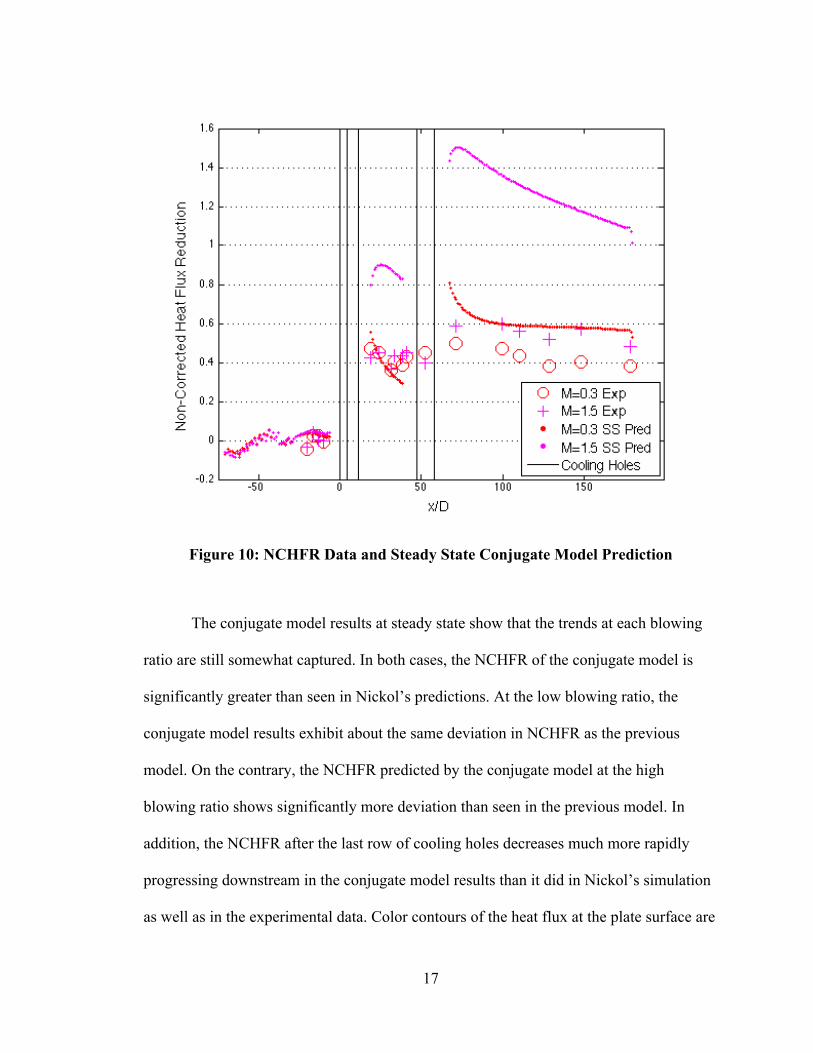
The conjugate model developed in this study was also run at steady state at the
high and low blowing ratios, and ran for 2,000 iterations. The absolute heat flux results of
these simulations also exhibited significant from the experimental data. The NCHFR of
these results was also computed and is plotted in Figure 10.
17
Figure 10: NCHFR Data and Steady State Conjugate Model Prediction
The conjugate model results at steady state show that the trends at each blowing
ratio are still somewhat captured. In both cases, the NCHFR of the conjugate model is
significantly greater than seen in Nickol’s predictions. At the low blowing ratio, the
conjugate model results exhibit about the same deviation in NCHFR as the previous
model. On the contrary, the NCHFR predicted by the conjugate model at the high
blowing ratio shows significantly more deviation than seen in the previous model. In
addition, the NCHFR after the last row of cooling holes decreases much more rapidly
progressing downstream in the conjugate model results than it did in Nickol’s simulation
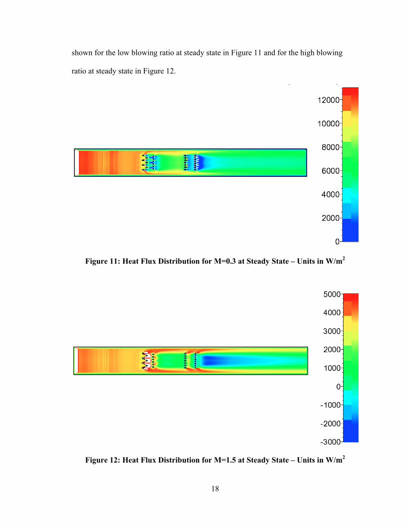
as well as in the experimental data. Color contours of the heat flux at the plate surface are
18
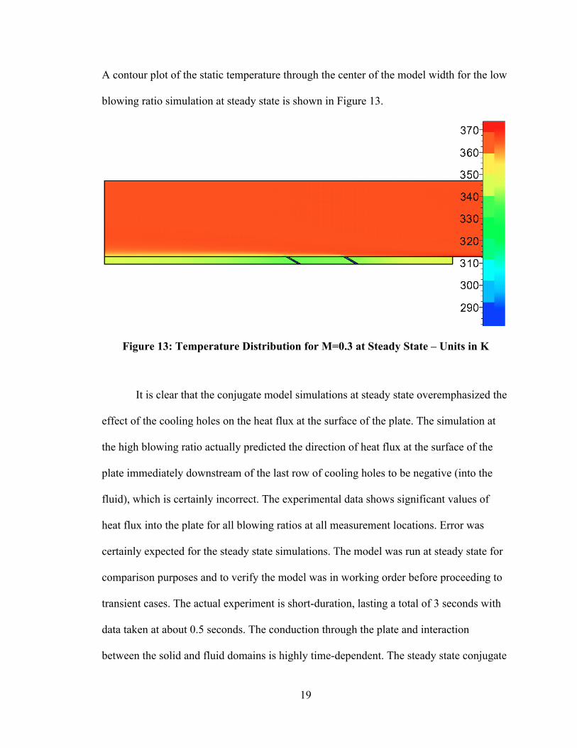
shown for the low blowing ratio at steady state in Figure 11 and for the high blowing
ratio at steady state in Figure 12.
Figure 11: Heat Flux Distribution for M=0.3 at Steady State – Units in W/m2
Figure 12: Heat Flux Distribution for M=1.5 at Steady State – Units in W/m2
19
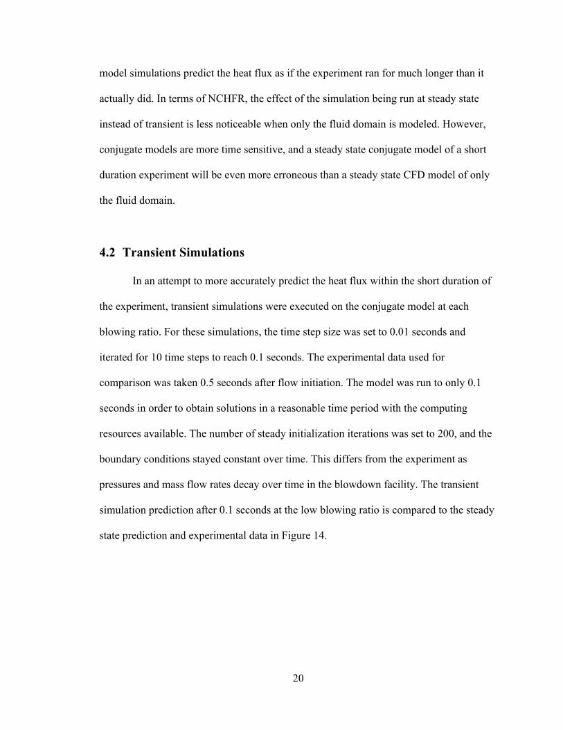
A contour plot of the static temperature through the center of the model width for the low
blowing ratio simulation at steady state is shown in Figure 13.
Figure 13: Temperature Distribution for M=0.3 at Steady State – Units in K
It is clear that the conjugate model simulations at steady state overemphasized the
effect of the cooling holes on the heat flux at the surface of the plate. The simulation at
the high blowing ratio actually predicted the direction of heat flux at the surface of the
plate immediately downstream of the last row of cooling holes to be negative (into the
fluid), which is certainly incorrect. The experimental data shows significant values of
heat flux into the plate for all blowing ratios at all measurement locations. Error was
certainly expected for the steady state simulations. The model was run at steady state for
comparison purposes and to verify the model was in working order before proceeding to
transient cases. The actual experiment is short-duration, lasting a total of 3 seconds with
data taken at about 0.5 seconds. The conduction through the plate and interaction
between the solid and fluid domains is highly time-dependent. The steady state conjugate
20
model simulations predict the heat flux as if the experiment ran for much longer than it
actually did. In terms of NCHFR, the effect of the simulation being run at steady state
instead of transient is less noticeable when only the fluid domain is modeled. However,
conjugate models are more time sensitive, and a steady state conjugate model of a short
duration experiment will be even more erroneous than a steady state CFD model of only
the fluid domain.
4.2 Transient Simulations
In an attempt to more accurately predict the heat flux within the short duration of
the experiment, transient simulations were executed on the conjugate model at each
blowing ratio. For these simulations, the time step size was set to 0.01 seconds and
iterated for 10 time steps to reach 0.1 seconds. The experimental data used for
comparison was taken 0.5 seconds after flow initiation. The model was run to only 0.1
seconds in order to obtain solutions in a reasonable time period with the computing
resources available. The number of steady initialization iterations was set to 200, and the
boundary conditions stayed constant over time. This differs from the experiment as
pressures and mass flow rates decay over time in the blowdown facility. The transient
simulation prediction after 0.1 seconds at the low blowing ratio is compared to the steady
state prediction and experimental data in Figure 14.
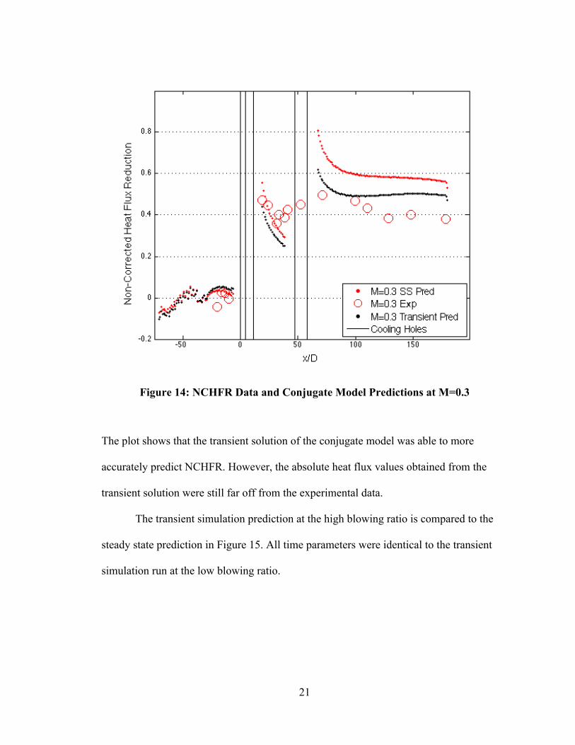
21
Figure 14: NCHFR Data and Conjugate Model Predictions at M=0.3
The plot shows that the transient solution of the conjugate model was able to more
accurately predict NCHFR. However, the absolute heat flux values obtained from the
transient solution were still far off from the experimental data.
The transient simulation prediction at the high blowing ratio is compared to the
steady state prediction in Figure 15. All time parameters were identical to the transient
simulation run at the low blowing ratio.
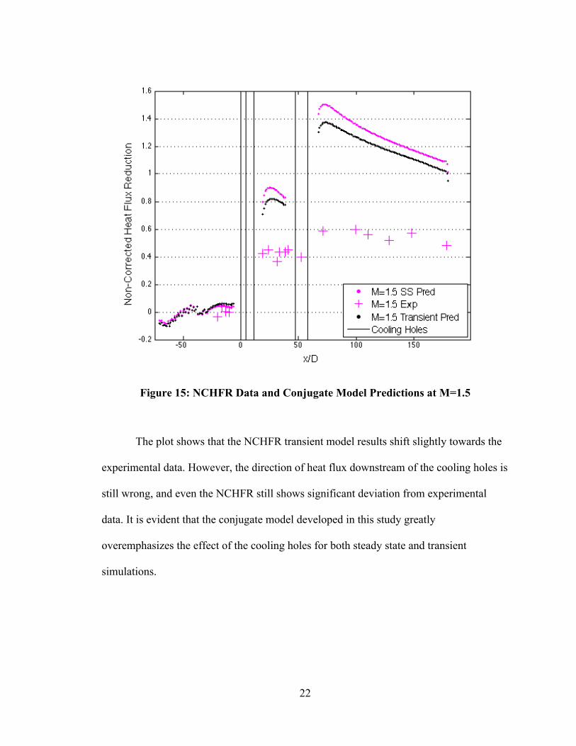
22
Figure 15: NCHFR Data and Conjugate Model Predictions at M=1.5
The plot shows that the NCHFR transient model results shift slightly towards the
experimental data. However, the direction of heat flux downstream of the cooling holes is
still wrong, and even the NCHFR still shows significant deviation from experimental
data. It is evident that the conjugate model developed in this study greatly
overemphasizes the effect of the cooling holes for both steady state and transient
simulations.
23
Chapter 5 CONCLUSION
5.1 Final Statements
When developing conjugate CFD models of short duration experiments, transient
simulations will generally yield more accurate predictions than steady state simulations.
This was expected, and is due to the time dependency of the solid conduction and
interaction between the fluid and solid domains. Conjugate models run at steady state will
calculate results as if the experiment was run over a long duration.
The conjugate model heat flux results were much less accurate at the high
blowing ratio than the low blowing ratio for both the steady state and transient cases. At
the high blowing ratio, the cooling air has much more of an effect on the conduction
through the solid. The conduction through the solid may have been modeled very
inaccurately due to the adiabatic conditions of the solid walls.
5.2 Future Work
Although the NCHFR of the low blowing ratio transient simulation was a slight
improvement from Nickol’s predictions, the heat flux results of the conjugate model still
exhibited significant deviation from the data. There is still a great deal of room for
improvement in the CFD model. The transient cases investigated in this study still used
constant boundary conditions over time. The actual experiment runs in a blowdown

24
facility with pressures and mass flow rates changing over time. A transient conjugate
model that applies variable boundary conditions and uses the correct time parameters
may be able to more accurately determine the heat flux over the surface of the plate.
Furthermore, the solver was unable to successfully run a case with the external
solid walls set as isothermal. These walls had to be set to adiabatic to obtain solutions,
and this could have greatly affected the results. It would be suggested to collaborate with
the Numeca support team and determine how to run a conjugate model with the solid
walls modeled isothermal.
25
REFERENCES
[1] Nickol, J.B., “Heat Transfer Measurements and Comparisons for a Film Cooled
Flat Plate with Realistic Hole Pattern in a Medium Duration Blowdown Facility,”
M.S. thesis, Department of Mechanical and Aerospace Engineering, The Ohio
State University, 2013.
[2] Bernasconi, S.L., "Design, Instrumentation and Study on a New Test Section for
Turbulence and Film Effectiveness Research in a Blowdown Facility", M.S.
Thesis, Department of Mechanical Engineering, The Ohio State University, 2007.
[3] Davis, S.M., "Heat-Flux Measurements for a Realistic Cooling Hole Pattern and
Different Flow Conditions", M.S. Thesis, Department of Mechanical and
Aerospace Engineering, The Ohio State University, 2011.
[4] Spalart, P.R. and Allmaras, S.R., 1992, "A One-Equation Turbulence Model for
Aerodynamic Flows," AIAA-92-0439, 30th Aerospace Sciences Meeting &
Exhibit, Reno, NV, USA.