congestion management and optimal placement of tcsc...
TRANSCRIPT
154
CHAPTER 5
CONGESTION MANAGEMENT AND OPTIMAL
PLACEMENT OF TCSC FOR TRANSFER
CAPABILITY ENHANCEMENT
5.1 INTRODUCTION
In the previous chapter the importance and computation of available
transfer capability are discussed. This chapter gives an introduction to
deregulated energy market, congestion and methods of congestion
management. A method to determine the optimal location of TCSC is also
proposed to enhance the transfer capability which is needed to meet the
rapidly changing demand of competitive markets.
Power system load growth is increasing at a faster rate as
compared to the increase in transmission capability. In the last decade
the increase in transmission capacity is approximately 50% of the
increased generation capacity. This has forced the system to move large
amount of power over transmission system and created challenges
associated with it. In the present open access system where anybody can
buy or sell energy there is a heavy transmission utilization in certain
areas which was not planned initially. This has increased the need of
improvements in the transfer capability of the system while maintaining
the system security and reliability.

155
The other reasons for short fall of transmission capability are
Difficulty in getting right of way permissions due to property
devaluation.
Health hazards due to electromagnetic effects.
Large impact on land use.
Ecological system effects.
Capital cost involved in construction and maintenance of new
lines and lack of investors for the proposed projects.
All the above mentioned factors and rapid growth of the load lead to
congestion of the system.
The challenge of transferring power over the existing grids has
created an interest among the researches in recent years for developing a
more robust power system applying new technologies. The concept and
application of flexible AC transmission systems (FACTS) to power system
was first initiated by Hingorani [127]. FACTS devices have the ability to
allow power systems to operate in a more economic, secure, flexible, and
sophisticated way. This chapter presents a brief discussion on different
methods and proposes an innovative technique for location of FACTs
device using complex valued neural network. This technique aims
towards effect of incorporating FACTS device TCSC on the real and
reactive power flows of that particular line and also on the transfer
capability of the system.
156
5.2 METHODS OF INCREASING TRANSFER CAPABILITY
The system transmission capability can be improved by using
primary methods involving system upgrading. Some traditional methods
are
Reconductoring transmission lines with larger size conductor of
higher power carrying capability and replacing terminal
equipment.
Voltage upgrade i.e. by increasing operating voltage of a
transmission line. This method requires up gradation of towers,
substations, circuit breakers, transformers and other equipment.
Installation of new transmission lines to alleviate overloads by
providing additional path.
Conversion from single line to double circuit by modifying the
tower structure.
By series compensation using a series capacitor in long distance
transmission lines.
Installing phase angle regulators.
Using small inertia generators and dispersed generation.
Insertion of switching stations along the transmission line.
Installing FACTS devices.
157
5.3 FLEXIBLE AC TRANSMISSION SYSTEMS (FACTS)
With the advent of flexible ac transmission system (FACTS) devices
power utilities all over the world are able to improve the system stability
limit, control the power flow, improve the transmission system security
and provide strategic benefits for better utilization of the existing power
system. The operation of FACTS devices is based on power electronic
controllers. These devices are also used to enhance transfer capability
and to minimize the total power loss of a system thereby improving the
system efficiency. In a competitive electric power system the most
important aspect is better utilization of existing lines in the context of
growing demand and outgrowth of energy trading markets. In the
context of restructuring the existing power systems FACTS devices have
assumed an importance since they can expand the usage potential of
transmission systems by controlling power flows in the network. FACTS
devices are operated in a manner so as to ensure that the contractual
requirements are fulfilled as far as possible by minimizing line
congestion. The main device considered here is Thyristor controlled
series capacitor (TCSC) for enhancement of transfer capability. Series
compensation is usually a preferable altenrative for increasing power flow
capability of lines compared to shunt compensators as the ratings
required for series compensators are significantly smaller.

158
5.3.1 TYPES OF FACTS CONTROLLERS
FACTS controllers are classified as series controllers, shunt
controllers, combined series–series controllers and combined series-
shunt controllers.
5.3.2 SERIES CONTROLLERS
These devices are connected in series with the lines to control the
reactive and capacitive impedance there by controlling or damping
various oscillations in a power system. The effect of these controllers is
equivalent to injecting voltage phasor in series with the line to produce or
absorb reactive power. Examples are Static Synchronous Series
Compensator (SSSC), Thyristor controlled Series Capacitor (TCSC),
Thyristor-Controlled Series Reactor (TCSR). . They can be effectively used
to control current and power flow in the system and to damp system’s
oscillations.
5.3.3 SHUNT CONTROLLERS
Shunt controllers inject current in to the system at the point of
connection. The reactive power injected can be varied by varying the
phase of the current. The examples are Static Synchronous Generator
(SSG), Static VAR Compensator (SVC).
5.3.4 COMBINED SERIES-SERIES CONTROLLERS
This controller may have two configurations consisting of series
controllers in a coordinated manner in a transmission system with multi
lines or an independent reactive power controller for each line of a multi

159
line system. An example of this type of controller is the Interline Power
Flow Controller (IPFC), which helps in balancing both the real and
reactive power flows on the lines.
5.3.5 COMBINED SERIES-SHUNT CONTROLLERS
In this type of controller there are two unified controllers a shunt
controller to inject current in to the system and a series controller to
inject series voltage. Examples of such controllers are UPFC and
Thyristor- Controlled Phase-Shifting Transformer (TCPST).
5.4 MODELING OF FLEXIBLE AC TRANSMISSION SYSTEM (FACTS)
DEVICES
For the enhancement of available transfer capability using FACTS
controllers it is assumed that the time constant of these devices is
negligible hence only static models are considered. The static models of
some of FACTS devices are explained below. Thyristor Controlled Series
Compensator (TCSC) is one such device which offers smooth and flexible
control for security enhancement with much faster response compared to
the traditional control devices [96,104,118]. Among the various FACTS
controllers, TCSC is considered for the proposed method in this chapter.
The detailed model of TCSC and brief discussion is given below.
5.4.1 THYRISTOR CONTROLLED SERIES COMPENSATOR (TCSC)
Thyristor controlled series compensator (TCSC) are connected in
series with transmission lines. It is equivalent to a controllable reactance
inserted in series with a line to compensate the effect of the line

160
inductance. The net transfer reactance is reduced and leads to an
increase in power transfer capability. The voltage profile as also improved
due to the insertion of series capacitance in the line. Series
compensation is usually a preferable alternative for increasing power flow
capability of lines as compared to shunt compensators as the ratings
required for series compensators are significantly smaller.
The transmission line model with a TCSC connected between the
two buses i and j is shown in Figure 5.1. Equivalent pi model is used to
represent the transmission line. TCSC can be considered as a static
reactance of magnitude equivalent to -jXc. The controllable reactance Xc
is directly used as control variable to be implemented in power flow
equation.
Fig. 5.1 Model of transmission line

161
Fig. 5.2 Model of TCSC
Fig. 5.3 Injection model of TCSC
The following equations are used to model TCSC.
Let the voltages at bus i and bus j are represented by iiV and
jjV
The complex power from bus i to j is
iijiijijij IVQPS ** (5.1)
)()(*
ciijjii jBVYVVV (5.2)
)()]([ **
ijijjicijiji jBGVVBBjGV (5.3)
Where
)(1
CLLijij jXjXR
jBG
(5.4)
162
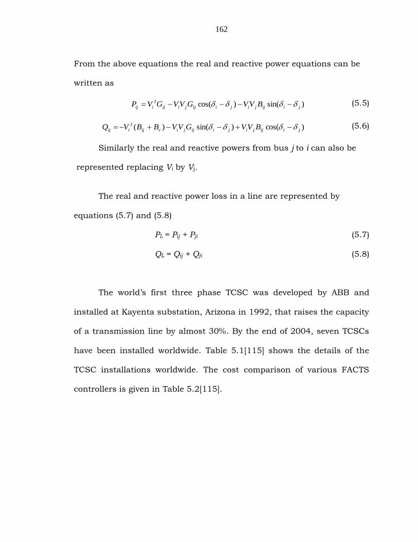
From the above equations the real and reactive power equations can be
written as
)sin()cos(2
jiijjijiijjiijiij BVVGVVGVP (5.5)
)cos()sin()(2
jiijjijiijjicijiij BVVGVVBBVQ (5.6)
Similarly the real and reactive powers from bus j to i can also be
represented replacing Vi by Vj.
The real and reactive power loss in a line are represented by
equations (5.7) and (5.8)
PL = Pij + Pji (5.7)
QL = Qij + Qji (5.8)
The world’s first three phase TCSC was developed by ABB and
installed at Kayenta substation, Arizona in 1992, that raises the capacity
of a transmission line by almost 30%. By the end of 2004, seven TCSCs
have been installed worldwide. Table 5.1[115] shows the details of the
TCSC installations worldwide. The cost comparison of various FACTS
controllers is given in Table 5.2[115].

163
Table 5.1 List of TCSC Installations
S.No. Year
Installed Country
Voltage
Level(kV) Purpose Place
1 1992 USA 230 To increase power
transfer capability
Kayenta Substation,
Arizona
2 1993 USA 500 Controlling line flow
and increased loading
C.J.Slatt substation,
Northern Oregon
3 1998 Sweden 400 Sub-synchronous
resonance mitigation Stode
4 1999 Brazil 500 To damp inter-area low
frequency oscillation
Imperatrz and Sarra de
Mesa
5 2002 China 500
Stability improvement,
low-frequency
oscillation mitigation
Pinguo substation,
Guangzhou
6 2004 India 400
Compensation,
Damping inter regional
power oscillation
Raipur substation
7 2004 China 220
Increase stability
margin, suppress low
frequency oscillation
North-West China power
system
Table 5.2 Cost of conventional and FACTS Controllers
S. No. FACTS Controllers
Cost (US $)
1 Shunt Capacitor 8/kVAr
2 Series Capacitor 20/kVAr
3 SVC 40/kVAr Controlled portions
4 TCSC 40/kVAr Controlled portions
5 STATCOM 50/kVAr
6 UPFC Series Portions 50/kVAr through power
7 UPFC Shunt Portions 50/kVAr controlled
164
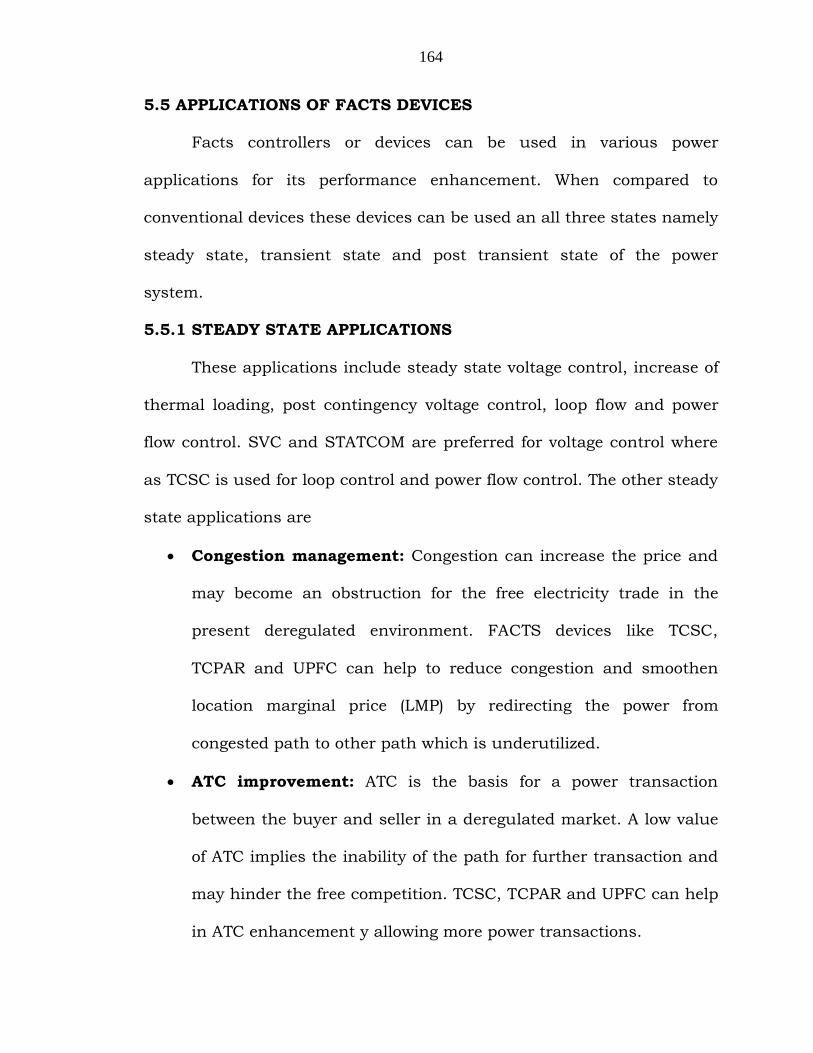
5.5 APPLICATIONS OF FACTS DEVICES
Facts controllers or devices can be used in various power
applications for its performance enhancement. When compared to
conventional devices these devices can be used an all three states namely
steady state, transient state and post transient state of the power
system.
5.5.1 STEADY STATE APPLICATIONS
These applications include steady state voltage control, increase of
thermal loading, post contingency voltage control, loop flow and power
flow control. SVC and STATCOM are preferred for voltage control where
as TCSC is used for loop control and power flow control. The other steady
state applications are
Congestion management: Congestion can increase the price and
may become an obstruction for the free electricity trade in the
present deregulated environment. FACTS devices like TCSC,
TCPAR and UPFC can help to reduce congestion and smoothen
location marginal price (LMP) by redirecting the power from
congested path to other path which is underutilized.
ATC improvement: ATC is the basis for a power transaction
between the buyer and seller in a deregulated market. A low value
of ATC implies the inability of the path for further transaction and
may hinder the free competition. TCSC, TCPAR and UPFC can help
in ATC enhancement y allowing more power transactions.

165
Reactive power and Voltage control: SVC, STATCOM can be use
for this purpose.
Loading Margin Improvement: Voltage collapse occurring at the
maximum loadability (nose point) is the main cause of recent world
wide block outs. The maximum transfer capability of a power
system can be improved by using shunt compensators efficiently.
Power flow and balancing control: TCSC, SSSC, UPFC can be
used to enable the load flow through parallel lines and there by
efficient utilization of lines can be made possible.
5.5.2 DYNAMIC APPLICATIONS
In these applications FACTS devices are used to enhance transient
stability by providing fast and rapid response, oscillation damping
dynamic control of voltage during contingencies to alleviate the system
from voltage collapse and sub synchronous resonance mitigation. These
devices are also used for inter connecting power systems for exchanging
the power between the regions over a long distance.
Congestion management
FACTS devices are used for relieving the system from congestion.
They can be used in a line such that least cost generators can be
dispatched more thereby reducing the price.
5.6 ELECTRICITY MARKET DEREGULATION AND CONGESTION
Deregulation and privatization of energy market has a wide range
of impact on the present day power systems around the world. The main

166
objective of the deregulation of power industry is to introduce
competition among the power producers and prevent monopolies.
Deregulation has increased complexity of the system as any body can
participate in the transactions to sell or buy electricity. As market
participants can produce and consume energy in amounts, transmission
lines are operated beyond their capacities causing congestion. It may
occur due to lack of coordination between generation and transmission
utilities. A congestion force higher cost generation in a network and has
direct impact on the economics therefore congestion management has
become very essential in a deregulated power system.
5.6.1 METHODS OF CONGESTION MANAGEMENT
The recent restructuring of energy system with existing generation
and transmission resources requires new methods for congestion
management and it also provides an opportunity for these approaches.
Allocation of transmission resources to support the competitive electricity
market is the current area of interest. Various new approaches are
proposed and being implemented which will provide feedback about their
suitability and contribution in improving the efficiency and reliability.
The two methods used for congestion management are
1. Cost free methods: Outaging of congested lines, adjusting
transformer taps, phase shifters or FACTS devices. The marginal
costs involved in their usage are nominal.
167
2. Non-cost free methods: Re-dispatch of generation, load or
transaction curtailment.
5.6.2 NETWORK CONGESTION MANAGEMENT USING TCSC
APPROACH
In recent years, deregulation of electric industry in the world has
created competitive markets to trade electricity. For deregulated
transmission network, one of the major consequences of the
nondiscriminatory open access requirement is substantial increase of
power transfers. Congestion management of deregulated transmission
network is important to accomplish non discriminative network access.
In this example congestion management approach using TCSC is
demonstrated considering a 5 bus system (Annexure – 1). This approach
aims at maximization of transmission margin without changing
contracted power. In this approach TCSC modeled as a variable
reactance is used. In order to check the validity of the proposed method
of congestion management, numerical results for a 5-bus system [5] are
shown in Figures 5.4, 5.5 and 5.6.
168
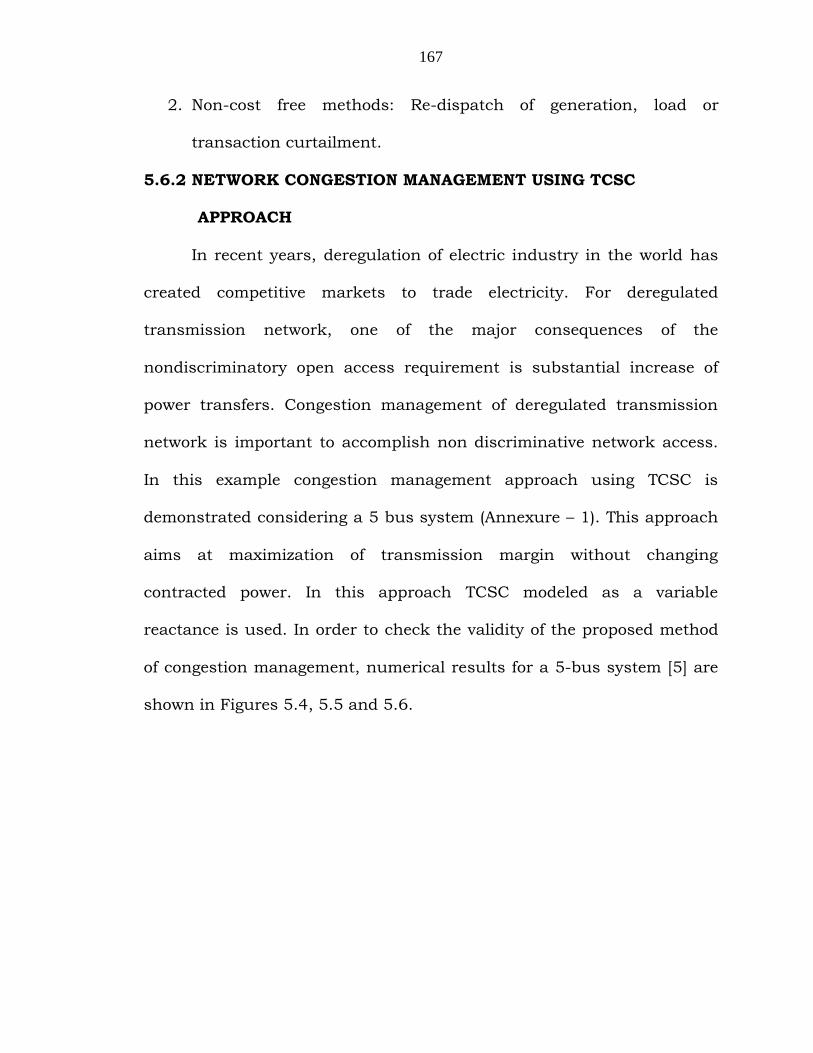
Fig. 5.4 Transmission margins without TCSC
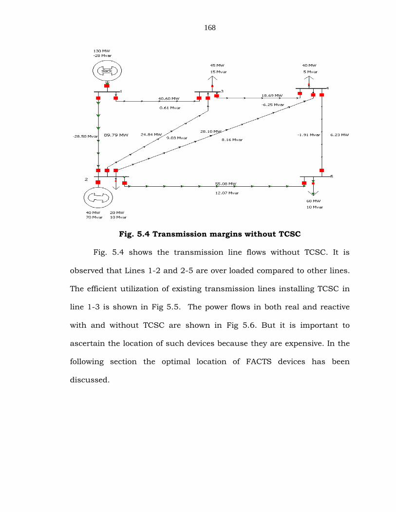
Fig. 5.4 shows the transmission line flows without TCSC. It is
observed that Lines 1-2 and 2-5 are over loaded compared to other lines.
The efficient utilization of existing transmission lines installing TCSC in
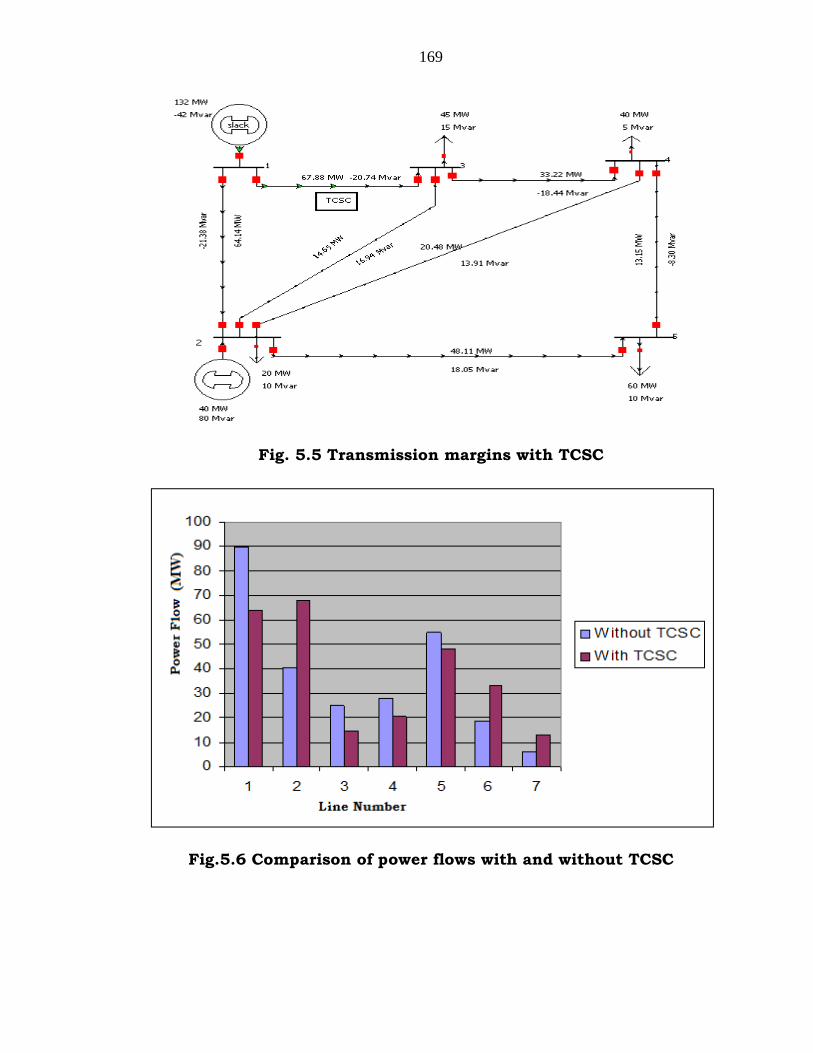
line 1-3 is shown in Fig 5.5. The power flows in both real and reactive
with and without TCSC are shown in Fig 5.6. But it is important to
ascertain the location of such devices because they are expensive. In the
following section the optimal location of FACTS devices has been
discussed.
169
Fig. 5.5 Transmission margins with TCSC
Fig.5.6 Comparison of power flows with and without TCSC
170
5.6.3 ENERGY PRICING
The three different methods of energy pricing are
1. Uniform marginal pricing (UMP)
2. Zonal marginal pricing (ZMP)
3. Location marginal pricing (LMP)
In UMP method one price is set for whole region ignoring the line
limits, losses and the physics of the power flows. In ZMP a uniform price
is set for zone or a graphical region considering the transmission limits
on the paths between the zones.
5.6.4 LOCATION MARGINAL PRICING (LMP)
Location marginal pricing (LMP) is defined as the marginal cost of
supplying the next increment of electric demand at a specific location on
the electric power network taking in to account both generation marginal
cost and the physical aspects of the transmission system it calculates an
optimal dispatch considering all the above aspects. In this approach a
price is set for each node in the transmission system. This method is
considered to be the most efficient and it is also known as nodal price.
Optimal power flow solution yields the LMPs at various nodes and the
solution can be used to for different inputs.
In a highly congested system negative LMPs occur at one or more
buses which is demonstrated by taking a 5 bus system. Usually this
occurs when the LMPs at other congested buses are very high. In Fig. 5.7

171
[120] the various line flows, area costs and location marginal prices are
shown without system congestion.
Fig. 5.7 Five bus system with no constraints
Fig. 5.8 Congested system with high LMP

172
Fig. 5.8 shows a congested system and the nodal prices are high at bus
3, bus 4 and bus 5 which is due to increase in load at bus 5. High value
of LMP at some buses is mainly due to the congestion.
5.6.4.1 NEGATIVE LMP
Negative LMPs may also occur in a highly congested system. A case
of negative LMP is considered here taking the same 5 bus example. Fig.
5.9 demonstrates the negative LMPs with congestion in line connected
between bus 1 and bus 2. The value of LMP at bus 5 is negative with a
value of -22.45$/MWh this may be due to large value of LMP
621.45$/MWh at bus and 700.98$/MWh at bus 4. Serving an additional
load of 1 MW at negative LMP will reduce the operating costs. Congestion
can be mitigated by increasing the flows to the loads at theses buses to
allow counter flows. It can be shown that this method reduces the
operating costs.
Fig. 5.9 Congested system with negative LMP
173
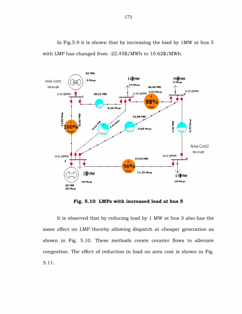
In Fig.5.9 it is shown that by increasing the load by 1MW at bus 5
with LMP has changed from -22.45$/MWh to 10.62$/MWh.
Fig. 5.10 LMPs with increased load at bus 5
It is observed that by reducing load by 1 MW at bus 3 also has the
same effect on LMP thereby allowing dispatch at cheaper generation as
shown in Fig. 5.10. These methods create counter flows to alleviate
congestion. The effect of reduction in load on area cost is shown in Fig.
5.11.

174
Fig. 5.11 LMPs with curtailed load at bus 3
5.6.4.2 TRANSMISSION LINE RELIEF (TLR) SENSITIVITIES
Transmission Line Relief sensitivities can be used for the purpose
of congestion alleviation by load curtailment. TLR sensitivities are
considered as inverse of power distribution factors (PTDFs). PTDFs are
used to determine the sensitivity of transmission line flow to a single
power transfer where as TLR sensitivity of the flow on single
transmission element to various transactions in the system. In the
method of congestion alleviation using load curtailment, TLR sensitivities
at all the load buses for the most overloaded line are considered

175
5.6.4.3 LOAD CURTAILMENT BASED ON TLR SENSITIVITIES
TLR sensitivity at a bus k for a congested line i - j is given by
equation
k
ijk
ijP
PS
(5.9)
Where
∆Pij is the excess power flow on line i - j
ijijij PPP (5.10)
Where
ijP : Actual power flow through line i - j
ijP : Flow limit of transmission line i - j
The new load new
kP at bus k can be obtained by
ijN
i
k
ij
k
ij
k
new
k P
S
SPP
1
(5.11)
Where
new
kP = Load after curtailment at bus k
Pk = Load before curtailment at bus k
k
ijS = sensitivity of power flow on line i - j due to load
change at bus k
N = Total number of load buses.

176
Table 5.3: TLR sensitivities
Bus
Congested Line i - j
1 - 2 2 - 5 3 - 4
1 0 0 0
2 -0.699 0.012 -0.104
3 -0.601 -0.023 0.208
4 -0.653 -0.064 -0.428
5 -0.676 -0.526 -0.266
Table 5.3 represents the TLR values of congested lines of a 5 bus
system. The higher the TLR sensitivity value more the effect of a single
MW power transfer at any bus. Based on these sensitivities load are
curtailed in required amounts at load buses in order to alleviate
congestion on the congested line i - j.
5.7 LOCATION OF FACTS DEVICE FOR TRANSFER CAPABILITY
ENHANCEMENT
The performance of power system can be improved considerably by
incorporating FACTS devices without changing the topology of the system
or generation reschedules [105-107]. These controllable devices are used
to decrease the system transmission congestion and increase the
available transfer capability. In recent years there is an increased
concern in these controllers essentially due to the development of higher

177
rating power electronic devices and secondly the need of control of power
transactions due to the deregulation.
The objective for the location of FACTS device may be one of the
following:
1. To allow a reduction in the real power loss of a particular line.
2. To improve the efficiency by reducing the total system real power
loss.
3. To reduce reactive power loss of the total system.
4. For congestion management and to provide maximum relief of
congestion in the system.
For the first three objectives, methods based on the sensitivity
approach may be used. If the objective of FACTS device placement is to
provide maximum relief of congestion, the devices may be placed in the
most congested lines or, alternatively, in locations determined by trial-
and-error.
A number of methods are proposed for optimal location of these
devices [108-112]. Sensitivity approach [108] based on line loss has been
proposed for placement of series capacitors, phase shifters and static
VAR (Volt Ampere Reactive) compensators. In [109][110] optimization
with different objective functions is discussed for optimal power flow with
FACTS devices. In [113][114], economic dispatch problem including cost
of the FACTS devices is solved to obtain the optimal locations of FACTS
devices. In this method it is assumed that initially these devices are

178
included in all the lines. In a vertically integrated power system several
methods can be used for determining the optimal location of the FACTS
devices. In Reference [108] for location of series capacitors and SVCs loss
sensitivity based approach is proposed. In reference [103] Continuation
Power flow method is used to determine the size and location of the
series compensator to increase the power transfer capability.
Various objective functions are proposed in [109][110] for optimal
power formulation in a deregulated environment using FACTS devices. In
reference [115] performance index is used which incorporates two factors
sensitivity matrix of TCSC with respect to congested line and shadow
pricing corresponding to the congested line for optimal location of TCSC
for reducing congestion cost. Genetic algorithm based approach is
presented in Reference [100] for the optimal location of the devices in a
distribution system. In [116] particle swarm optimization algorithm is
used to determine the optimal location of various FACTS devices in a
power system in order to relieve the lines from over loads. Bees Algorithm
is proposed for the optimal location of FACTS controllers in Ref [101].
Peerapol Jirapong, Weerakorn Ongsakul [117] presented Hybrid
Evolutionary Algorithm for optimal location of multi type FACTS devices.
In Reference [118] a sensitivity factor based approach for the optimal
placement of the TCSC to minimize the congestion cost is presented. The
sensitivity factor is based on the ratio of change in real power flow to the
base case power flow in the most congested line.

179
5.8 INDICES USED FOR THE DETERMINATION OF LOCATION OF
FACTS DEVICES
There are different sensitivities used for finding the optimal
location of FACTS devices. The main criterion may be reduction in total
power loss or increase in maximum power transmittable or voltage
stability. The power flow between the buses is given by
SinX
VVP
ij
ji
ij (5.12)
Where Vi and Vj are the voltages of buses i and j
δ is the angle and
Xij is the reactance of the line
From the above equation it is clear that the transient stability of
the system can be controlled by varying the reactance.
In following section determination of reactive power loss sensitivity
factor is discussed. This factor and the proposed method of finding the
location of TCSC is compared in the subsequent sections.
5.8.1 REACTIVE POWER LOSS SENSITIVITY
The reactive power loss is affected by change in reactance of the
line by using compensators such as facts devices. This effect can be
utilized to devise reactive power sensitivity index. This index is basically
the change in reactive power loss with respect to line reactance.
The reactive power loss of Kth line between buses i and j is
jijijikkloss CosVVVVBQ 222
)( (5.13)
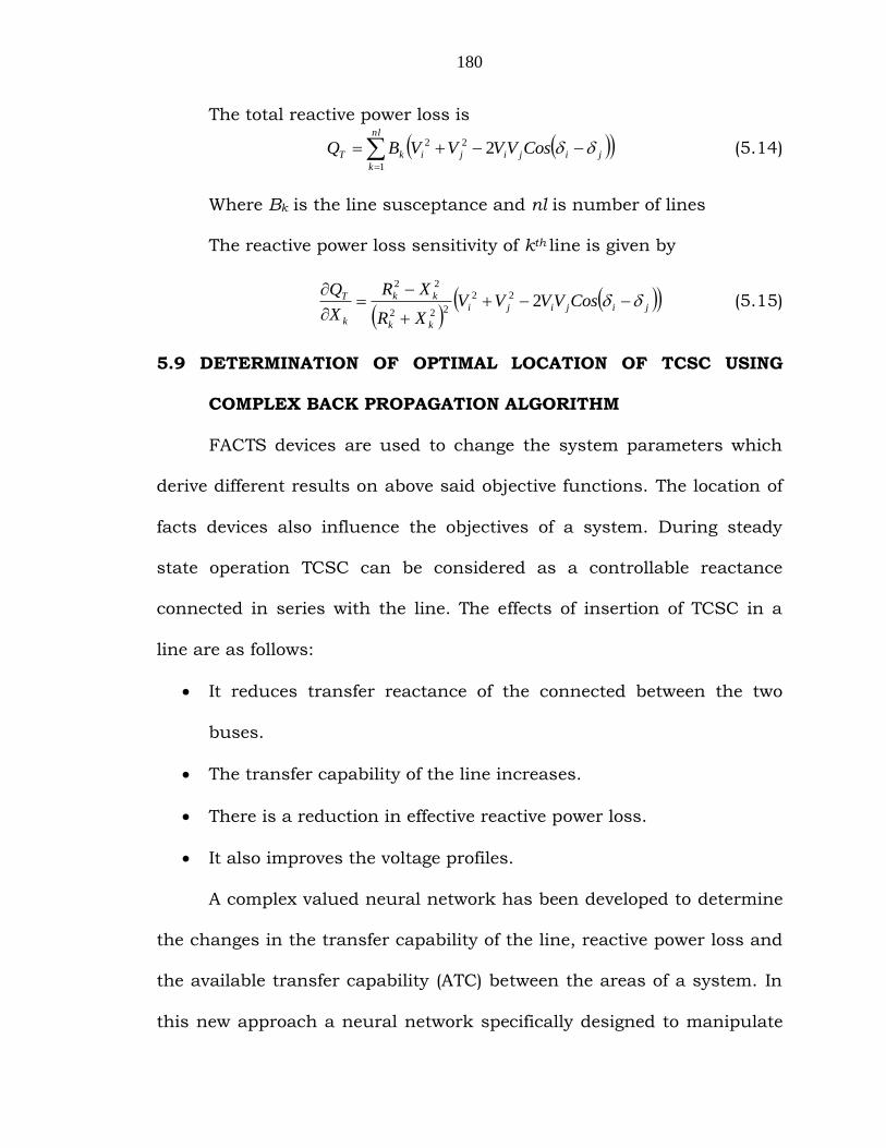
180
The total reactive power loss is
nl
k
jijijikT CosVVVVBQ1
22 2 (5.14)
Where Bk is the line susceptance and nl is number of lines
The reactive power loss sensitivity of kth line is given by
jijiji
kk
kk
k
T CosVVVVXR
XR
X
Q
222
222
22
(5.15)
5.9 DETERMINATION OF OPTIMAL LOCATION OF TCSC USING
COMPLEX BACK PROPAGATION ALGORITHM
FACTS devices are used to change the system parameters which
derive different results on above said objective functions. The location of
facts devices also influence the objectives of a system. During steady
state operation TCSC can be considered as a controllable reactance
connected in series with the line. The effects of insertion of TCSC in a
line are as follows:
It reduces transfer reactance of the connected between the two
buses.
The transfer capability of the line increases.
There is a reduction in effective reactive power loss.
It also improves the voltage profiles.
A complex valued neural network has been developed to determine
the changes in the transfer capability of the line, reactive power loss and
the available transfer capability (ATC) between the areas of a system. In
this new approach a neural network specifically designed to manipulate
181
the complex numbers in electrical power engineering is described. This
newly developed approach requires lesser number of input neurons or
nodes, lesser converging time and less prone to local minima problems
when compared to the conventional neural networks using real numbers.
5.9.1 OPTIMAL LOCATION OF TCSC IN A 14 BUS SYSTEM
The performance of a network can be improved considerably
without topological changes or generation rescheduling by controlling
power flows using FACTS devices. The insertion of such devices can
alleviate the system congestion and improve transfer capability. To
demonstrate the effectiveness of the proposed complex valued neural
network approach a 14 bus and 30 bus systems are considered.
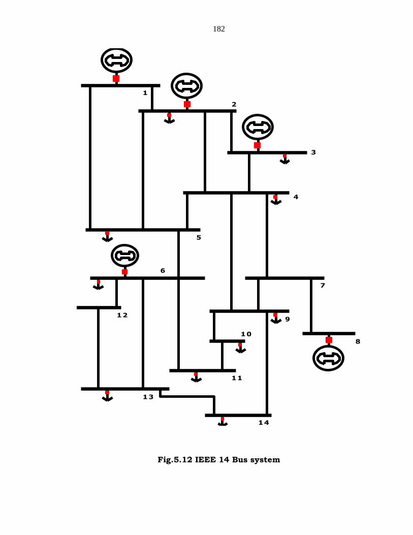
IEEE 14 bus system [120] consists of 5 generators, 20 lines
(Annexure – 1) as shown in Fig. 5.12. Among these lines 15 lines shown
in Table 5.4 are considered for the location of TCSC as the real power
loss of the other lines is zero. For a smaller power system with less
number of buses, optimal location can be determined taking one line at a
time. Repeated power flow (RPF) method is used to compute the transfer
capability of each line with and without incorporating TCSC. The various
objectives considered for the location of FACTS devices are explained in
section 5.6. Here transfer capability, real and reactive power losses are
considered to be the main objectives that are influenced by the value and
the location of the FACTS device.
182
1
2
3
4
5
6
7
8
9
10
11
12
13
14
Fig.5.12 IEEE 14 Bus system

183
TABLE 5.4 Location of TCSC
S. No. Line S. No. Line
1 Line 1-2 9 Line 6-12
2 Line 1-5 10 Line 6-13
3 Line 2-3 11 Line 9-10
4 Line 2-4 12 Line 9-14
5 Line 2-5 13 Line 11-10
6 Line 3-4 14 Line 12- 13
7 Line 5-4 15 Line 13-14
8 Line 6-11
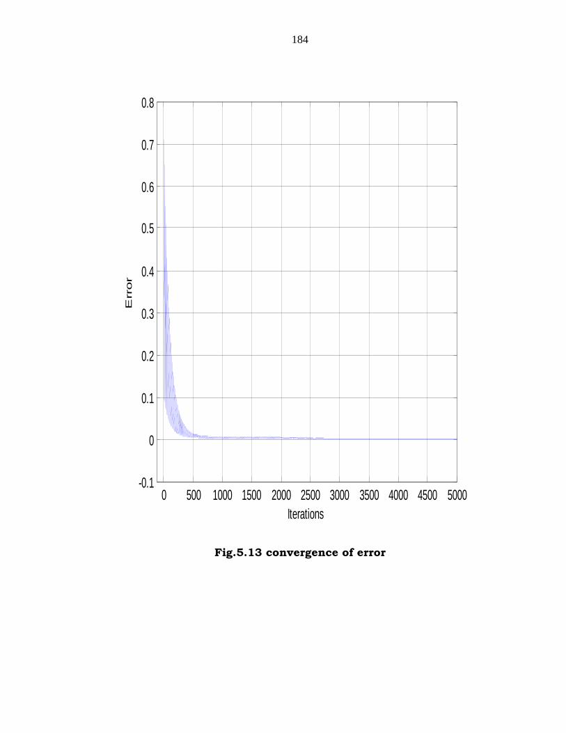
5.9.2 TRAINING PHASE
In this phase a total of 105 training samples are generated and
used to train the proposed complex valued neural network. If the number
of training patterns are increased more accurate predictions are obtained
but over training may lead to memorization. RPF method is used for this
purpose. As the effect of TCSC inserted in a transmission line is
equivalent to a controllable reactance in series with the line which
changes the system parameters, line admittances in complex form are
taken as the inputs to the neural network. It is found that a learning rate
of 0.011 is adequate for achieving a mean squared error of 0.01. The
convergence of error is shown in Figure 5.13.
184
0 500 1000 1500 2000 2500 3000 3500 4000 4500 5000-0.1
0
0.1
0.2
0.3
0.4
0.5
0.6
0.7
0.8
Iterations
Error
Fig.5.13 convergence of error

185
Figure.5.14 Line Real Power loss with TCSC
As discussed earlier the real power loss varies with amount of
compensation. There are 15 lines and each line reactance is varied from
20% to 80% in steps. Figure 5.14 shows the change in real power loss in
all the 15 lines with various amounts of compensation. The first bar of
each line represents the real power loss without any compensation.

186
Fig.5.15 Line Reactive Power loss with TCSC
Reactive power depends on the line reactance as shown in Eq.
5.15. The effect of change in reactance on reactive power loss is
calculated at various values. The total reactive power loss of the system
at maximum loadable point with different line compensations in all 15
lines is shown in Figure 5.15.
187
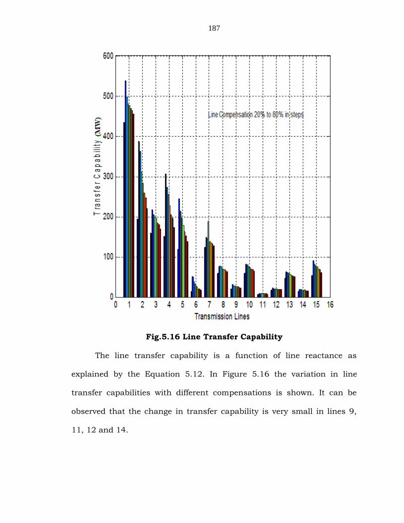
Fig.5.16 Line Transfer Capability
The line transfer capability is a function of line reactance as
explained by the Equation 5.12. In Figure 5.16 the variation in line
transfer capabilities with different compensations is shown. It can be
observed that the change in transfer capability is very small in lines 9,
11, 12 and 14.
188
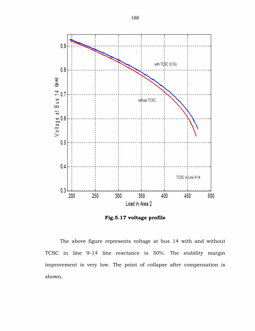
Fig.5.17 voltage profile
The above figure represents voltage at bus 14 with and without
TCSC in line 9-14 line reactance is 50%. The stability margin
improvement is very low. The point of collapse after compensation is
shown.

189
Fig.5.18 voltage profile
The above Figure 5.18 represents voltage at bus 14 with and
without TCSC in line 9-14. The line reactance compensation is 80% in
this case. Stability margin and point of voltage collapse can be improved
by changing the compensation.
190
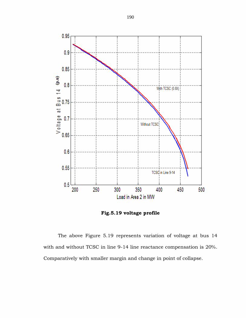
Fig.5.19 voltage profile
The above Figure 5.19 represents variation of voltage at bus 14
with and without TCSC in line 9-14 line reactance compensation is 20%.
Comparatively with smaller margin and change in point of collapse.

191
Fig.5.20 Voltage profile at Bus 14
The above Figure 5.20 represents voltage at bus 14 with and
without TCSC in line 13-14 line reactance compensation is 80%. It can
be seen that the there is a noticeable change in stability margin. Point of
collapse is also changed when TCSC is installed in this line.
192
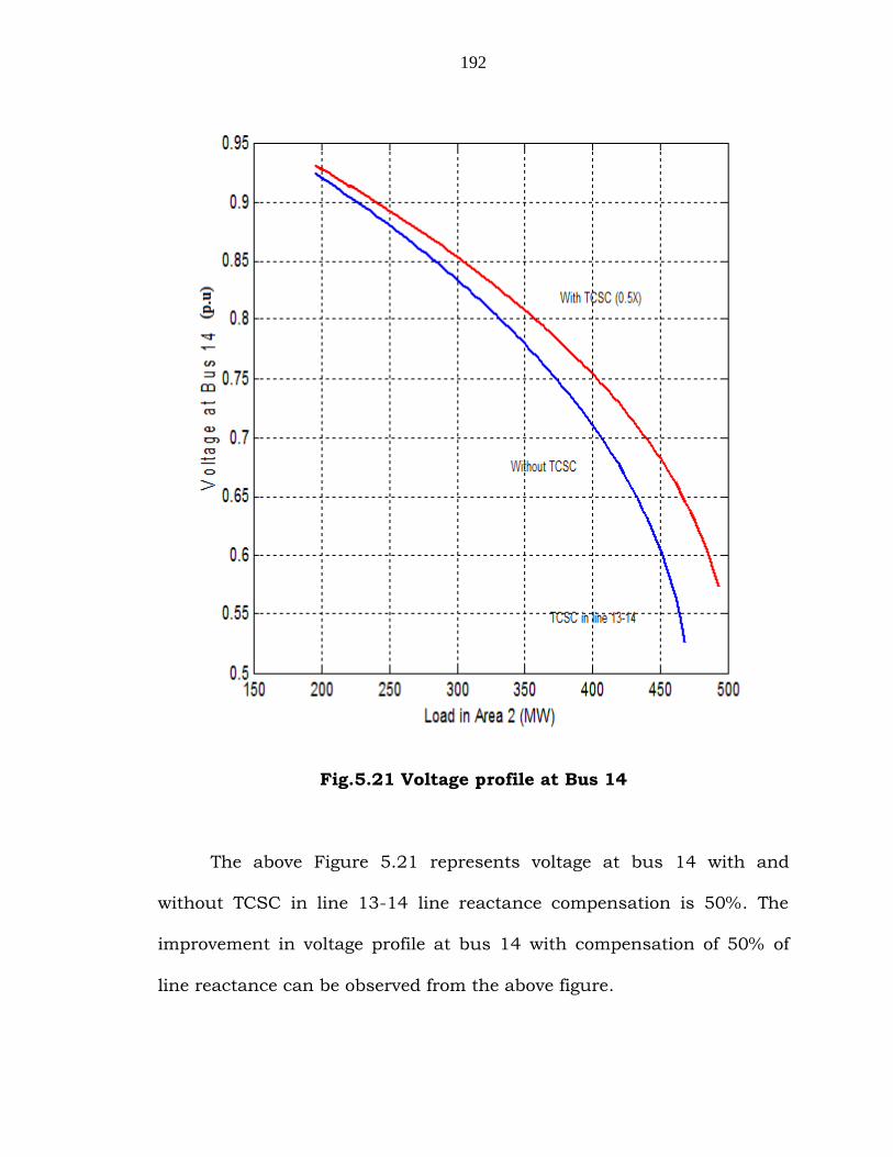
Fig.5.21 Voltage profile at Bus 14
The above Figure 5.21 represents voltage at bus 14 with and
without TCSC in line 13-14 line reactance compensation is 50%. The
improvement in voltage profile at bus 14 with compensation of 50% of
line reactance can be observed from the above figure.

193
5.9.3 RESULTS AND DISCUSSIONS OF 14 BUS SYSTEM
The proposed complex valued neural network method is tested for
different values of compensation in the lines 1-5, 2-3, 2-5, 3-4 and 5-4.
The results are shown in Tables 5.4 to 5.9. All the values are represented
in per unit. It is observed that this method is very efficient to determine
the location of the FACTS devices.
Table 5.5 (a) Results with various compensations in line 1-5
Compensation 25 %
Compensation 30%
CVNN RPF (NR) CVNN RPF (NR)
Line Flow
0.2305 + j0.0568 0.2300+j0.0690 0.2371+j0.0558 0.2390+j0.0680
Total Loss
0.1398 + j0.4837 0.1390+j0.4950i 0.1411+j0.4838 0.1390+j0.4860
Table 5.5 (b) Results with various compensations in line 1-5
Compensation 45 %
Compensation 55%
CVNN RPF (NR)
CVNN RPF (NR)
Line Flow
0.2654+j0.0522 0.2710+j0.0600 0.2944+j0.0494 0.2970+j0.0510
Total Loss
0.1464+j0.4839 0.1390+j0.4600 0.1519+j0.4840 0.1410+j0.4420
Table 5.6 (a) Results with various compensations in line 2-3
Compensation 25 % Compensation 30%
CVNN RPF (NR)
CVNN RPF (NR)
Line Flow
0.1825-j0.0706 0.1730-j0.0560 0.1831-j0.0739 0.1760-j0.0590
Total Loss
0.1409+j0.4990 0.1390+j0.5070 0.1410+j0.4987 0.1390+j0.5030
194
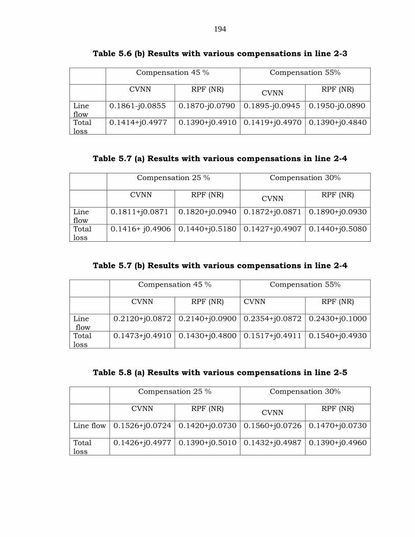
Table 5.6 (b) Results with various compensations in line 2-3
Compensation 45 %
Compensation 55%
CVNN RPF (NR) CVNN
RPF (NR)
Line flow
0.1861-j0.0855 0.1870-j0.0790 0.1895-j0.0945 0.1950-j0.0890
Total loss
0.1414+j0.4977 0.1390+j0.4910 0.1419+j0.4970 0.1390+j0.4840
Table 5.7 (a) Results with various compensations in line 2-4
Compensation 25 %
Compensation 30%
CVNN RPF (NR)
CVNN RPF (NR)
Line flow
0.1811+j0.0871 0.1820+j0.0940 0.1872+j0.0871 0.1890+j0.0930
Total loss
0.1416+ j0.4906 0.1440+j0.5180 0.1427+j0.4907 0.1440+j0.5080
Table 5.7 (b) Results with various compensations in line 2-4
Compensation 45 % Compensation 55%
CVNN RPF (NR) CVNN RPF (NR)
Line flow
0.2120+j0.0872 0.2140+j0.0900 0.2354+j0.0872 0.2430+j0.1000
Total loss
0.1473+j0.4910 0.1430+j0.4800 0.1517+j0.4911 0.1540+j0.4930
Table 5.8 (a) Results with various compensations in line 2-5
Compensation 25 %
Compensation 30%
CVNN RPF (NR) CVNN
RPF (NR)
Line flow 0.1526+j0.0724 0.1420+j0.0730 0.1560+j0.0726 0.1470+j0.0730
Total loss
0.1426+j0.4977 0.1390+j0.5010 0.1432+j0.4987 0.1390+j0.4960

195
Table 5.8 (b) Results with various compensations in line 2-5
Compensation 45 % Compensation 55%
CVNN RPF (NR) CVNN
RPF (NR)
Line flow 0.1699+j0.0733 0.1700+j0.0750 0.1836+j0.0737 0.1860+j0.0730
Total loss
0.1454+j0.5017 0.1460+j0.5120 0.1476+j0.5036 0.1470+j0.5000
Table 5.9 (a) Results with various compensations in line 3-4
Compensation 25 %
Compensation 30%
CVNN RPF (NR)
CVNN RPF (NR)
Line flow 0.0258+j0.1440 0.0160+j0.1120 0.0260+j0.1449 0.0190+j0.1200
Total loss
0.1512+j0.5309 0.1390+j0.5030 0.1514+j0.5319 0.1460+j0.5280
Table 5.9 (b) Results with various compensations in line 3-4
Compensation 45 %
Compensation 55%
CVNN RPF (NR)
CVNN RPF (NR)
Line flow 0.0269+j0.1472 0.0250+j0.1390 0.0277+j0.1483 0.0300+j0.1560
Total loss
0.1522+j0.5347 0.1500+j0.5340 0.1531+j0.5360 0.1560+j0.5460
Table 5.10 (a) Results with various compensations in line 5-4
Compensation 25 %
Compensation 30%
CVNN RPF (NR) CVNN
RPF (NR)
Line flow 0.1347+j0.0412 0.1300+j0.0470 0.1408+j0.0447 0.1310+j0.0470
Total loss
0.1829+j0.4473 0.1390+j0.5180 0.2011+j0.4584 0.1390+j0.5160
196
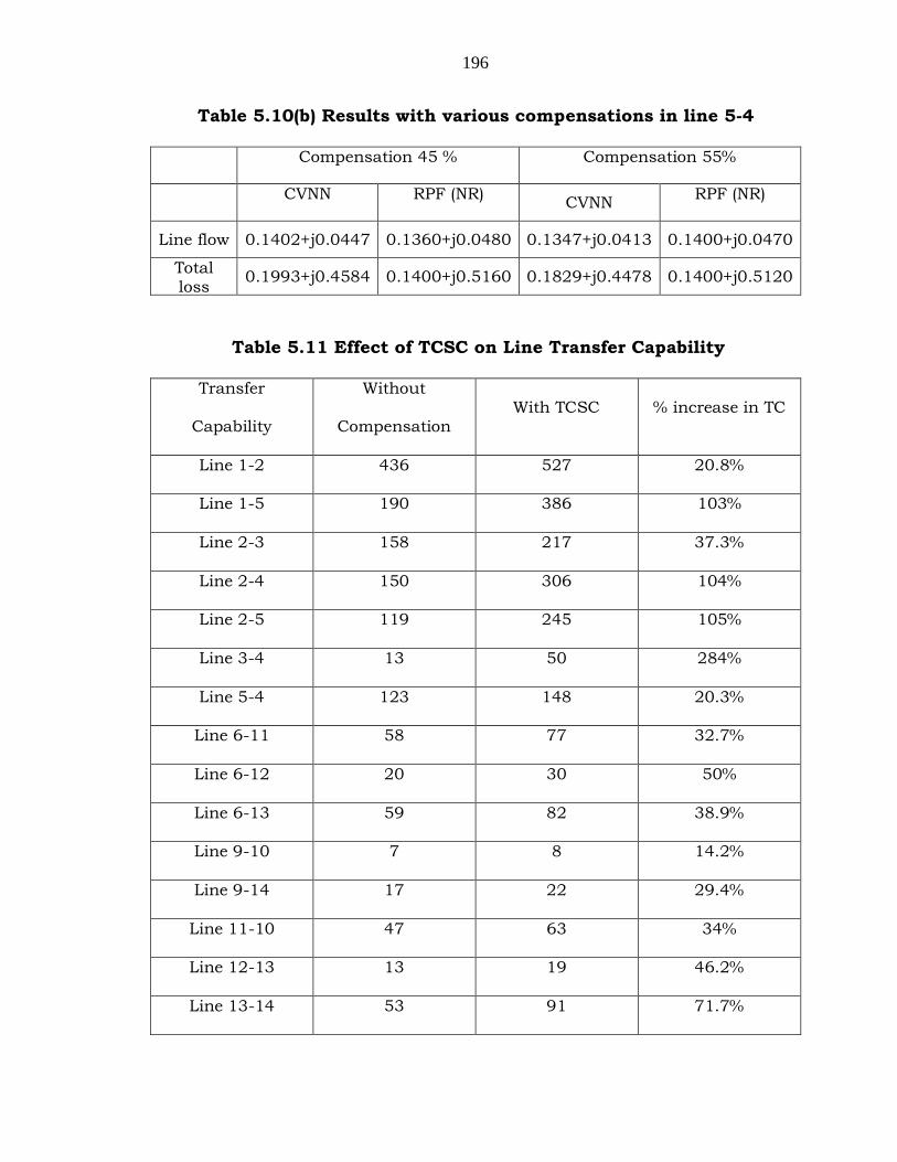
Table 5.10(b) Results with various compensations in line 5-4
Compensation 45 %
Compensation 55%
CVNN RPF (NR)
CVNN RPF (NR)
Line flow 0.1402+j0.0447 0.1360+j0.0480 0.1347+j0.0413 0.1400+j0.0470
Total loss
0.1993+j0.4584 0.1400+j0.5160 0.1829+j0.4478 0.1400+j0.5120
Table 5.11 Effect of TCSC on Line Transfer Capability
Transfer
Capability
Without
Compensation
With TCSC % increase in TC
Line 1-2 436 527 20.8%
Line 1-5 190 386 103%
Line 2-3 158 217 37.3%
Line 2-4 150 306 104%
Line 2-5 119 245 105%
Line 3-4 13 50 284%
Line 5-4 123 148 20.3%
Line 6-11 58 77 32.7%
Line 6-12 20 30 50%
Line 6-13 59 82 38.9%
Line 9-10 7 8 14.2%
Line 9-14 17 22 29.4%
Line 11-10 47 63 34%
Line 12-13 13 19 46.2%
Line 13-14 53 91 71.7%
197
The effect of TCSC on line transfer capability is shown in Table
5.11. It is seen that there is a large change in transfer capability of some
lines when considered individually.
5.10 ENHANCEMENT OF ATC IN A MODIFIED IEEE 30 BUS SYSTEM
In this section modified IEEE 30 bus system (Annexure – 1) has
been considered for simulation studies. In an open access deregulated
environment the power transaction can occur from any point of
generation to any point of load. The single line diagram of 30 bus system
is shown in Figure 5.22. Some typical transactions considered are
between area 1 to area 2 and area 1 to area 3 for illustration purpose.
Repeated power flow method is used and in all the transactions
considered here the real and reactive powers are increased at a constant
power factor. To train the network and to test its robustness a number of
patterns are generated with different values of compensations
incorporating TCSC in each of the four tie lines as shown in Figure 5.22.
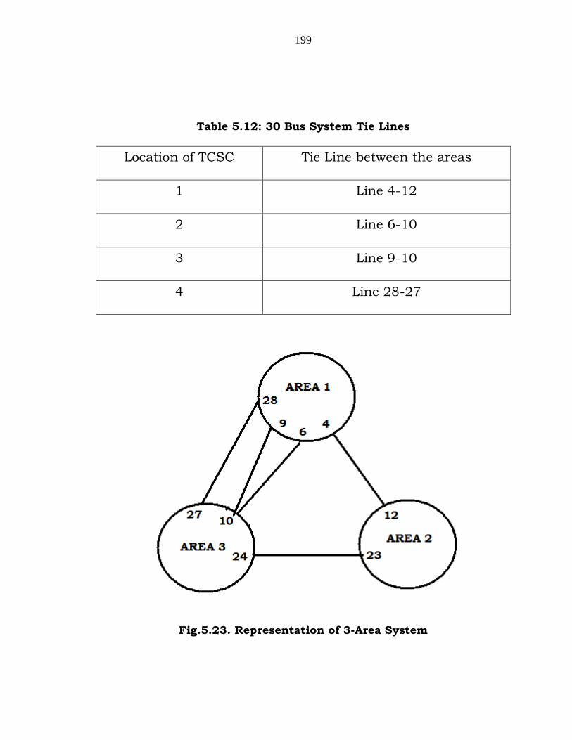
The 3 areas of the system are shown in Figure 5.23. Line parameters are
considered as inputs to the network and it is assumed that these
transaction paths have a small amount of line resistances, otherwise
product of weighted inputs would become zero. Various locations of
TCSC are also show in the Figure 5.24 [128] and Table 5.10.

198
Fig.5.22 Modified IEEE 30 Bus System
199
Table 5.12: 30 Bus System Tie Lines
Location of TCSC Tie Line between the areas
1 Line 4-12
2 Line 6-10
3 Line 9-10
4 Line 28-27
Fig.5.23. Representation of 3-Area System
200
5.10.1 ALGORITHM FOR THE PROPOSED APPROACH
The procedure followed for the determination of Transfer capability
and available transfer capability is explained in the following steps.
1. Newton Raphson power flow method is used to obtain the base
case results.
2. Area 1 is assumed to be the seller area, Area 2 and Area 3 as
buyer areas.
3. The load and the generation are increased in steps.
4. Nose curve or PV curves are traced using Repeated Power flow
which is explained in section [5.5.3].
5. The sum of power flows through the tie lines at the point of
voltage collapse are taken as Total transfer capability.
6. At this voltage limit the Available Transfer Capability is obtained
from
ATCmn = Pij – Pij0 (5.16)
7. The enhancement of ATC with different compensations can be
obtained incorporating the model of TCSC in the method used.
The following transactions are considered for estimating the ATC of
the system.
1. Transaction 1 between Area 1 and Area 2 in which Area 1
supplies the increase in load in Area 2.
2. Transaction 2 between area 1 and Area 3 in which Area 1
supplies the increased load in area 3.
201
The various effects of incorporating TCSC in each of the 4 tie lines
are simulated using the mathematical model of TCSC and used for
training and validation of proposed method.
Line 23-24 is not considered as it is between area 2 and area 3. That
is not between buyer and seller areas.
5.10.2 RESULTS AND DISCUSSIONS
The proposed method has been applied to IEEE 14 bus system and
a modified IEEE 30 bus system to find the optimum location of the
TCSC. In this work on TCSC is modeled and considered because it
reduces net transfer reactance and enhances power transfer capability.
As discussed earlier the added advantage of series compensator TCSC is
its smaller rating compared to shunt compensators. It is observed that
there is an improvement in voltage profile and also reduction in line loss
and total loss of the system. For optimum location of TCSC the selection
criteria can be one of the parameters explained in section 5.7.

202
Fig.5.24 Line Transfer Capability
Figure 5.24 shows the variation of transfer capability with TCSC
placed in lines 4-12, 6-10, 9-10 and 28-27. Each TCSC is operated with
an inductive reactance varying from 20% to 80% of line reactance.
According to the results obtained it can be stated that the best
candidates for placing the TCSC controllers are those lines which have
largest change in power flow between the base case and the ATC point.
From the Figure 5.24 it can be observed that there a parabolic increase
in power flow with TCSC compensation in line 6-10.
203
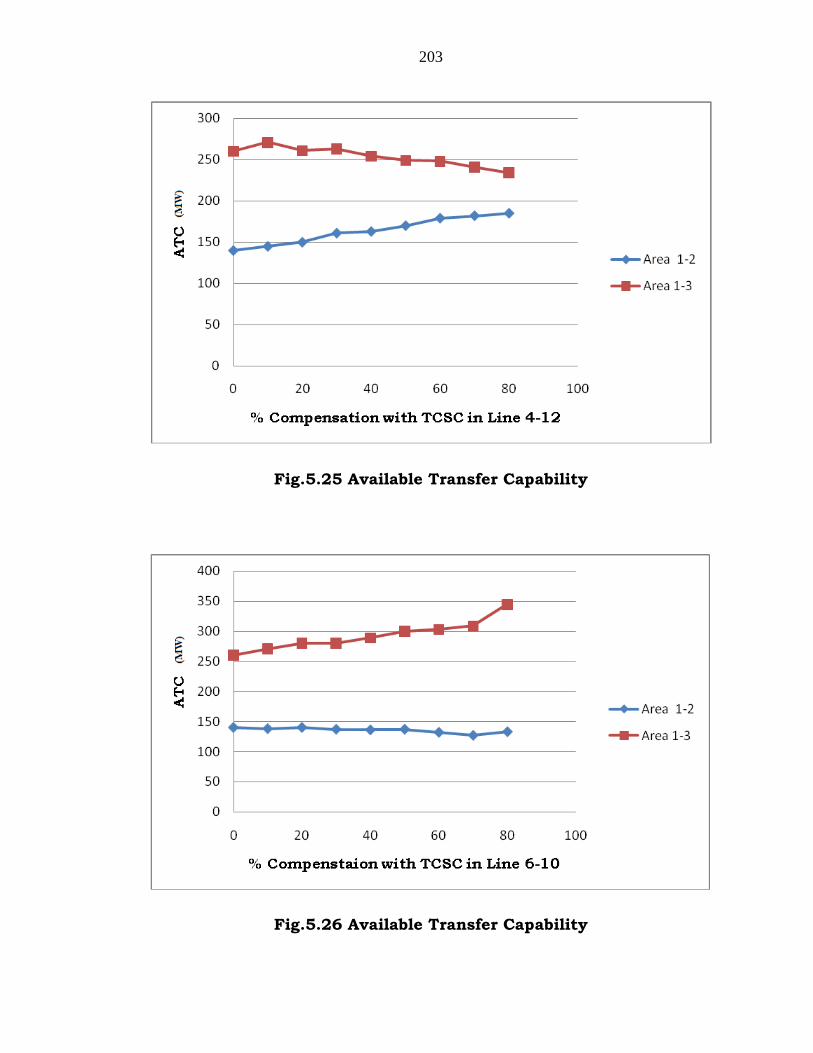
Fig.5.25 Available Transfer Capability
Fig.5.26 Available Transfer Capability

204
Fig.5.27 Available Transfer Capability
Fig.5.28 Available Transfer Capability
205
In figures 5.25 – 5.28 the change in available transfer capbility
from area 1 to 2 also area 1 to 3 are shown with respect to diffent values
and locations of TCSC. Again it is seen that there is a largest percentage
change (approximately 40%) in ATC1-3 when the TCSC is located in line
6-10.
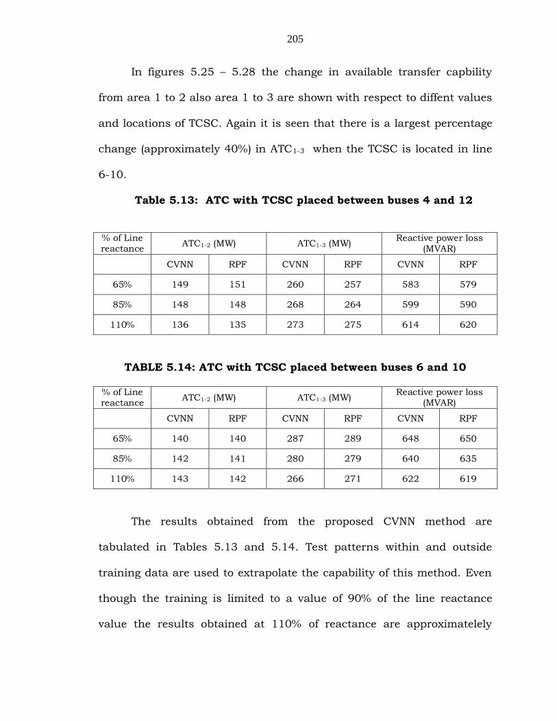
Table 5.13: ATC with TCSC placed between buses 4 and 12
% of Line reactance
ATC1-2 (MW) ATC1-3 (MW) Reactive power loss
(MVAR)
CVNN RPF CVNN RPF CVNN RPF
65% 149 151 260 257 583 579
85% 148 148 268 264 599 590
110% 136 135 273 275 614 620
TABLE 5.14: ATC with TCSC placed between buses 6 and 10
% of Line reactance
ATC1-2 (MW) ATC1-3 (MW) Reactive power loss
(MVAR)
CVNN RPF CVNN RPF CVNN RPF
65% 140 140 287 289 648 650
85% 142 141 280 279 640 635
110% 143 142 266 271 622 619
The results obtained from the proposed CVNN method are
tabulated in Tables 5.13 and 5.14. Test patterns within and outside
training data are used to extrapolate the capability of this method. Even
though the training is limited to a value of 90% of the line reactance
value the results obtained at 110% of reactance are approximatelely
206
same as that of conventional method. This method is used to generalize
the nonlinear relationship between the system parameters with series
compensation and the transfer capability, line loss and system total real
and reactive power loss.
5.10.3 LOCATION OF TCSC FOR REDUCTION OF SYSTEM TOTAL
REACTIVE POWER LOSS
In this section a method using sensitivity factor is used to find the
optimal location of TCSC. This method is based on the sensitivity of the
total system reactive power loss (QL) with respect to the variable that can
be controlled incorporating the FACTS devices. When a TCSC is placed in
series with the transmission line between the buses i and j it
compensates the line reactanace Xij. The reduction in transfer reactance
leads to increase in maximum power that can be transferred on the line
and also with a reduction in system effective reactive power loss.
The optimal location of TCSC can be found using the reactive
power loss sensitivity factor. With respect to the control variable that is
line reactance Xij incorporating TCSC between the i and j the loss
sensitivity factor is calculated as follows:
222
22
22
)()(2
ijij
ijij
jijiji
ij
Lij
XR
XRCosVVVV
X
Qa
(5.17)
207
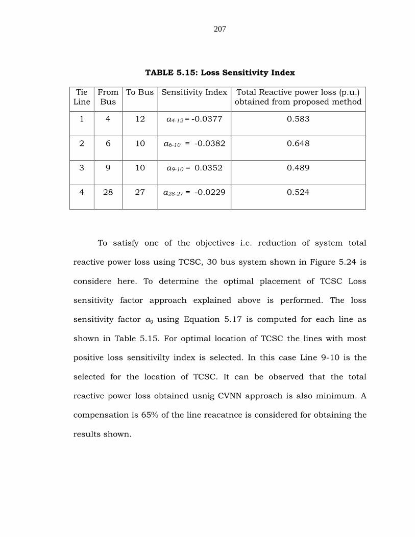
TABLE 5.15: Loss Sensitivity Index
Tie
Line
From
Bus
To Bus Sensitivity Index Total Reactive power loss (p.u.)
obtained from proposed method
1 4 12 a4-12 = -0.0377 0.583
2 6 10 a6-10 = -0.0382 0.648
3 9 10 a9-10 = 0.0352 0.489
4 28 27 a28-27 = -0.0229 0.524
To satisfy one of the objectives i.e. reduction of system total
reactive power loss using TCSC, 30 bus system shown in Figure 5.24 is
considere here. To determine the optimal placement of TCSC Loss
sensitivity factor approach explained above is performed. The loss
sensitivity factor aij using Equation 5.17 is computed for each line as
shown in Table 5.15. For optimal location of TCSC the lines with most
positive loss sensitivilty index is selected. In this case Line 9-10 is the
selected for the location of TCSC. It can be observed that the total
reactive power loss obtained usnig CVNN approach is also minimum. A
compensation is 65% of the line reacatnce is considered for obtaining the
results shown.

208
5.11 CONCLUSIONS
The present restructuring of electric power industry has created
most challenging problems with respect to operation and security of the
system. Recent deregulation of the energy market resulted heavy
transmission utilization. As discussed earlier the power system is over
loaded and the delay in new transmission projects has a great impact on
it causing overloading of transmission lines and voltage sags. In the
present open access deregulated environment, market participants can
produce and consume energy in amounts, transmission lines are
operated beyond their capacities causing congestion. Methods of
congestion management using TCSC and load curtailment are shown in
this chapter.
In situations stated above, increasing network security by
controlling power flow i.e. re-dispatching of power and injection of
reactive power play a vital role. There is also a need of improving transfer
capability while maintaining the security of the system. This necessity
has created interest among the researchers to propose cost effective
methods for a robust power system using the latest technologies. The
most suitable means for this purpose are FACTs devices which can
enhance the transfer capability, improve voltage profile and there by
network security. In contrast to the conventional compensators like
series, shunt capacitors and reactors which can be used for improvement
of transfer capability and voltage profile, FACTS devices have added

209
advantages of step less control for fine regulation, capability to increase
or decrease the power flow according to the requirement and their re-
locatability as they can be built in to movable containers.
In this chapter a method using complex valued neural networks is
proposed to determine optimal location of FACTS devices, particularly
TCSC considering requirements, such as reduction of loss, increasing
transfer capability and there by alleviating congestion in deregulated
electricity market. This method is particularly useful for the system
planners during the expansion procedure to determine the size and
location of FACTS devices as they provide most reliable and efficient
solution. It is shown that this method is very effective and easy to apply
in a deregulated system.