congestion control and fairness for real-time media ... · congestion control and fairness for ......
TRANSCRIPT

Master Thesis
Congestion Control andFairness for Real-time Media
Transmission
Submitted by
Juhi Kulshrestha
Submitted on
June 29, 2011
Supervisor
Prof. Dr.- Ing. Thorsten Herfet
Advisor
Manuel Gorius, M.Sc.
Reviewers
Prof. Dr.- Ing. Thorsten HerfetProf. Dr. Holger Hermanns
Saarland University
Faculty of Natural Sciences and Technology I
Department of Computer Science


Universität des Saarlandes
Postfach 15 11 50, 66041 Saarbrücken
UNIVERSITÄT DES SAARLANDES
Lehrstuhl für Nachrichtentechnik
FR Informatik
Prof. Dr. Th. Herfet
Universität des Saarlandes Campus Saarbrücken C6 3, 10. OG 66123 Saarbrücken
Telefon (0681) 302-6541 Telefax (0681) 302-6542
www.nt.uni-saarland.de
Master’s Thesis for Juhi Kulshrestha
Congestion Control and Fairness for Real-time Media Transmission
Audiovisual content generates the major part of the traffic in the Future Internet. Currently the Transmission Control Protocol (TCP) is the prevalent protocol for web-based audio and video distribution. It provides flow and congestion control, as well as perfect reliability. These features are essential for error-free file transfer and ensure fairness between concurrent transmissions over the Internet. However, without modification they reasonably affect the Quality of Experience (QoE) for real-time media streams, especially if they are transmitted over wireless networks.
Audiovisual applications require a predictable delivery time but can tolerate a specific residual error. With the generalized architecture on adaptive hybrid error correction1, the Telecommunications Lab has developed a versatile basis for efficient error correction on packet level. Coding parameters are determined analytically based on a statistical model in order to serve predictable transmission delay as well as predictable residual loss to the application.
The scope of this master's thesis is the design of a congestion control mechanism with respect to real-time media transmission that operates on top of the available error correction architecture. In particular, the tasks to be solved are the following:
• Introduce into available policies for congestion control and discuss their usability for real-time media. Consider scalability issues of those schemes for large receiver groups.
• The literature presents ideas based on predictive estimation of the available channel bandwidth for a smoother congestion control in TCP. Discuss those approaches for a potential solution.
• Develop a congestion control mechanism suitable for real-time media transmission on top of the generalized architecture on adaptive hybrid error correction.
• Demonstrate the solution in a suitable environment. An implementation of a media-oriented transport protocol is available at the Telecommunications Lab and should be the basis for practical demonstrations. Erroneous network behavior might be emulated via the netem2 network emulator on top of a physical IP network.
Tutor: Supervisor:
Manuel Gorius Prof. Dr.-Ing. Th. Herfet
1 http://www.nt.uni-saarland.de/publications/ 2 http://www.linuxfoundation.org/en/Net:Netem
—
–


Eidesstattliche Erklärung Ich erkläre hiermit an Eides Statt, dass ich die vorliegende Arbeit selbstständig verfasst und keine anderen als die angegebenen Quellen und Hilfsmittel verwendet habe.
Statement in Lieu of an Oath
I hereby confirm that I have written this thesis on my own and that I have not used any other media or materials than the ones referred to in this thesis.
Einverständniserklärung Ich bin damit einverstanden, dass meine (bestandene) Arbeit in beiden Versionen in die Bibliothek der Informatik aufgenommen und damit veröffentlicht wird.
Declaration of Consent I agree to make both versions of my thesis (with a passing grade) accessible to the public by having them added to the library of the Computer Science Department. Saarbrücken,…………………………….. …………………………………………. (Datum / Date) (Unterschrift / Signature)

ACKNOWLEDGEMENTS
First and foremost I would like to thank Prof. Dr.-Ing. Thorsten Herfet for his guidance
throughout our association. He always gave me invaluable advice and provided the best
work atmosphere one could possibly want.
Manuel Gorius is another person who played a significant role in shaping this work. I am
grateful for his much appreciated ideas, patience and constant support. This thesis wouldn’t
have been possible without the many discussions and brainstorming sessions that we had.
I would further like to thank all the people at the Telecommunications Lab at Saarland
University for being helpful and providing a conducive environment for doing research.
And last but not the least, I would like to thank my family for supporting me and being
there for me in every imaginable way.

viii

ABSTRACT
Real-time media already comprises of a large chunk of the Internet traffic, and its amount
is expected to increase even further in the coming years. In such a situation, where there
exist multiple simultaneous media streams, the questions of congestion control and fairness
gain even greater significance. In this Master thesis, these questions have been targeted and
the use of adaptive bandwidth estimation in ensuring fairness and controlling congestion
has been explored. By incorporating the estimate of the bandwidth in the network into the
parameter calculation for the Adaptive Hybrid Error Correction (AHEC) architecture, along
with the already existing delay and residual loss constraints, we propose to control the con-
gestion in the network. A differentiation between losses due to congestion and corruption
is expected to lead to a better bandwidth estimation in heterogeneous networks.
Keywords
Adaptive Hybrid Error Correction (AHEC), congestion control, bandwidth estimation, fair-
ness, future media internet

x

TABLE OF CONTENTS
ACKNOWLEDGEMENTS . . . . . . . . . . . . . . . . . . . . . . . . . . . . . . vii
ABSTRACT . . . . . . . . . . . . . . . . . . . . . . . . . . . . . . . . . . . . . . . ix
LIST OF TABLES . . . . . . . . . . . . . . . . . . . . . . . . . . . . . . . . . . . 3
LIST OF FIGURES . . . . . . . . . . . . . . . . . . . . . . . . . . . . . . . . . . 5
I INTRODUCTION . . . . . . . . . . . . . . . . . . . . . . . . . . . . . . . . . 7
1.1 Motivation . . . . . . . . . . . . . . . . . . . . . . . . . . . . . . . . . . . 7
1.2 State of the Art . . . . . . . . . . . . . . . . . . . . . . . . . . . . . . . . . 8
1.3 Thesis Outline . . . . . . . . . . . . . . . . . . . . . . . . . . . . . . . . . . 10
II ADAPTIVE HYBRID ERROR CORRECTION SCHEME . . . . . . . 13
2.1 Adaptive Hybrid Error Correction Architecture . . . . . . . . . . . . . . . 13
2.2 Analytical Design of Coding Parameters . . . . . . . . . . . . . . . . . . . 15
2.3 PRRT Prototype Implementation . . . . . . . . . . . . . . . . . . . . . . . 17
2.4 Evaluation of AHEC Architecture under Limited Bandwidth . . . . . . . 19
2.4.1 Evaluation of Original AHEC Architecture . . . . . . . . . . . . . . 20
2.4.2 Evaluation of Revised AHEC Architecture . . . . . . . . . . . . . . 20
III BANDWIDTH ESTIMATION & CONGESTION CONTROL . . . . . 23
3.1 Bandwidth Estimation Techniques . . . . . . . . . . . . . . . . . . . . . . . 23
3.1.1 Packet Pair/Train Dispersion (PPTD) . . . . . . . . . . . . . . . . 23
3.1.2 Variable Packet Size (VPS) probing . . . . . . . . . . . . . . . . . . 24
3.1.3 Self-Loading Periodic streams (SLoPS) . . . . . . . . . . . . . . . . 24
3.1.4 Trains of Packet Pairs (TOPP) . . . . . . . . . . . . . . . . . . . . 24
3.2 Congestion Control Mechanisms . . . . . . . . . . . . . . . . . . . . . . . . 25
3.2.1 Window-based congestion control protocols . . . . . . . . . . . . . 25
3.2.2 TCP - like congestion control protocols . . . . . . . . . . . . . . . . 28
3.2.3 Equation based congestion control protocols . . . . . . . . . . . . . 29
3.3 Summary . . . . . . . . . . . . . . . . . . . . . . . . . . . . . . . . . . . . . 30
3.4 TCP Friendly Rate Control (TFRC) Protocol . . . . . . . . . . . . . . . . 31
3.4.1 Loss Event Rate . . . . . . . . . . . . . . . . . . . . . . . . . . . . . 31
1
3.4.2 Model for TCP Throughput . . . . . . . . . . . . . . . . . . . . . . 31
3.4.3 Estimation of round-trip time and timeout value . . . . . . . . . . 33
3.4.4 Estimation of loss event rate . . . . . . . . . . . . . . . . . . . . . 33
3.4.5 Bandwidth Estimation using TFRC . . . . . . . . . . . . . . . . . . 35
3.4.6 TCP Friendly Multicast Congestion Control (TFMCC) Protocol . . 35
IV PROPOSED SOLUTION FOR INCLUSION OF BANDWIDTH LIMI-TATION . . . . . . . . . . . . . . . . . . . . . . . . . . . . . . . . . . . . . . . 37
4.1 Analytical Solution for Optimizing under Limited Bandwidth . . . . . . . 37
4.1.1 Adjusting channel coding rate . . . . . . . . . . . . . . . . . . . . . 38
4.1.2 Adjusting source coding rate . . . . . . . . . . . . . . . . . . . . . . 40
4.2 Proposed Architecture for Bandwidth Estimation using TFRC . . . . . . 41
4.2.1 Sender Functionalities . . . . . . . . . . . . . . . . . . . . . . . . . 43
4.2.2 Receiver Functionalities . . . . . . . . . . . . . . . . . . . . . . . . 46
4.3 Implementation Details . . . . . . . . . . . . . . . . . . . . . . . . . . . . . 52
4.3.1 Sender Implementation . . . . . . . . . . . . . . . . . . . . . . . . . 52
4.3.2 Receiver Implementation . . . . . . . . . . . . . . . . . . . . . . . . 53
V EVALUATION . . . . . . . . . . . . . . . . . . . . . . . . . . . . . . . . . . . 57
5.1 Experimental Setup . . . . . . . . . . . . . . . . . . . . . . . . . . . . . . 57
5.2 Results & Observations . . . . . . . . . . . . . . . . . . . . . . . . . . . . 59
VI DIFFERENTIATING CONGESTION AND CORRUPTION LOSSES 69
6.1 Need for loss differentiation . . . . . . . . . . . . . . . . . . . . . . . . . . 69
6.2 Available Loss Differentiation Techniques . . . . . . . . . . . . . . . . . . . 70
6.3 Integration with our solution - A Hint . . . . . . . . . . . . . . . . . . . . 70
VII CONCLUSION AND OUTLOOK . . . . . . . . . . . . . . . . . . . . . . . 73
7.1 Summary . . . . . . . . . . . . . . . . . . . . . . . . . . . . . . . . . . . . . 73
7.2 Future Work . . . . . . . . . . . . . . . . . . . . . . . . . . . . . . . . . . 73
2

LIST OF TABLES
1 Parameters of AHEC Scheme [13] . . . . . . . . . . . . . . . . . . . . . . . . 15
2 Optimum Parameter Sets for different values of Target Packet Loss Rate . . 39
3 Estimated Bandwidth: Comparison of results . . . . . . . . . . . . . . . . . 65
3

4

LIST OF FIGURES
1 AHEC Architecture [1] . . . . . . . . . . . . . . . . . . . . . . . . . . . . . . 14
2 PRRT module in Kernel User space1 . . . . . . . . . . . . . . . . . . . . . . 18
3 Queue structure of AHEC protocol stack[1] . . . . . . . . . . . . . . . . . . 18
4 Bandwidth peaks in throughput for pure FEC configuration . . . . . . . . . 21
5 Bandwidth peaks in throughput for HEC configuration . . . . . . . . . . . . 21
6 Data and Acknowledgement transmission of a TCP connection [6] . . . . . 26
7 An example of loss events and loss intervals . . . . . . . . . . . . . . . . . . 32
8 Residual loss as an objective function to be minimized under delay and band-width constraints . . . . . . . . . . . . . . . . . . . . . . . . . . . . . . . . . 38
9 Bandwidth (Residual RI) vs Reliability (Target PLR) . . . . . . . . . . . . 39
10 Functionalities of the sender and receiver in bandwidth estimation . . . . . 42
11 Measurement of Round Trip Time . . . . . . . . . . . . . . . . . . . . . . . 43
12 Token Bucket Filter . . . . . . . . . . . . . . . . . . . . . . . . . . . . . . . 46
13 Bottleneck Bandwidth Estimation . . . . . . . . . . . . . . . . . . . . . . . 48
14 Transition from Slow Start to Normal Operation Phase . . . . . . . . . . . 48
15 RTT averaging using EWMA factor of 0.1 . . . . . . . . . . . . . . . . . . . 49
16 RTT averaging using EWMA factor of 0.05 . . . . . . . . . . . . . . . . . . 50
17 RTT averaging using EWMA factor of 0.01 . . . . . . . . . . . . . . . . . . 50
18 Bandwidth Estimation using TCP Response Equation . . . . . . . . . . . . 51
19 Sender Functionality . . . . . . . . . . . . . . . . . . . . . . . . . . . . . . . 52
20 Receiver Functionality . . . . . . . . . . . . . . . . . . . . . . . . . . . . . . 56
21 Experimental Setup . . . . . . . . . . . . . . . . . . . . . . . . . . . . . . . 57
22 Experimental Setup with the bottleneck at the router . . . . . . . . . . . . 59
23 Observation Interval = 1 x RTT . . . . . . . . . . . . . . . . . . . . . . . . 60
24 Observation Interval = 1.5 x RTT . . . . . . . . . . . . . . . . . . . . . . . 61
25 Observation Interval = 2 x RTT . . . . . . . . . . . . . . . . . . . . . . . . 61
26 Observation Interval = 3 x RTT . . . . . . . . . . . . . . . . . . . . . . . . 62
27 Impact of retransmissions for error correction on sending rate . . . . . . . . 63
28 Experimental Setup with concurrent TCP streams . . . . . . . . . . . . . . 65
5

29 Impact of 1 competing TCP stream on sending rate . . . . . . . . . . . . . 66
30 Impact of 2 competing TCP streams on sending rate . . . . . . . . . . . . . 66
31 Impact of 5 competing TCP streams on sending rate . . . . . . . . . . . . . 67
32 Impact of 10 competing TCP streams on sending rate . . . . . . . . . . . . 67
33 Impact of 15 competing TCP streams on sending rate . . . . . . . . . . . . 68
34 Inclusion of Loss Differentiation into our Bandwidth Estimation Solution . 71
6
CHAPTER I
INTRODUCTION
The Internet today sees a huge traffic of multimedia transmission, and this has been a
compelling factor in the recent evolution of the Internet. The Cisco VNI Forecast [15]
predicts that by the year 2014, the various forms of video (TV, VoD, Internet Video and
P2P) will exceed 91% of the global consumer traffic. According to their Usage Study,
the subset of online video that includes streaming video, flash and Internet TV, already
comprises of 26% of the traffic today. Also the voice and video communication traffic is
now 6 times higher than the data communication traffic. With the advent of 3D video
and HD video, the bandwidth demands are expected to rise even further. It is thus, an
undeniable fact that the Internet is fast converging towards a Media Internet. And this
rapidly increasing demand of real time media services over Internet has led to the creation
of the Future Media Internet [16] concept.
Once dominated by text based data applications, currently the Internet has a major
part of its traffic occupied by the various types of audio-video media. The real time media
traffic on the Internet has different requirements as compared to the data traffic, even
though both rely on the underlying Internet Protocol (whether in its current version IPv4
or in the upcoming IPv6) encapsulation for the digital data transmission. Generally the
audio-visual applications and multimedia data impose certain constraints on delivery time
but can at the same time tolerate some losses, and this is not sufficiently made available
by the current protocols. ITU-T Y.1541 [17] is the most widely agreed recommendation
specifying the objectives of end-to-end network performance for IP based services and it
relates subjective QoS descriptions with IP network attributes like packet transfer delay,
delay variation, packet loss and error ratios and captures the results into a set of Network
QoS classes.
1.1 Motivation
With the definite shift in paradigm that can be seen on the Internet, and the multitude
of media streams being transmitted over it, congestion is a very real problem in today’s
Internet. And with the increasing amount of media content being transmitted, the situation
is expected to get even worse in the future. It is therefore extremely important to identify
the situation when the network is in a congested state. A general practice to over come
transmission losses is to add redundancy to the data being transmitted. But in a situation
where there is congestion developing in the network, the losses can not be reduced by
7

adding redundancy. In fact in congestion scenarios, adding redundancy would degrade the
performance further. Therefore to handle the congestion, we first need to recognize such a
situation and then accordingly take some action, for example, to notify the application of
the congestion and let it decide how to deal with it.
The stability of the Internet today is generally attributed to the fairness inherent to the
TCP protocol. But at the same time there are some applications like the real-time media
applications, which make use of UDP based protocols, which have no notion of fairness. The
UDP-based media streaming applications can be for both stored media content as well as
real time content. The technique for streaming the stored content is progressive download,
where the digital media content is downloaded and stored on the client side device before
being played, while for real time streaming applications a small buffer is used in order to
initiate playback, but at no point the entire media file is stored locally.
All the real time media applications that we are addressing in this thesis have a mini-
mum bandwidth requirement which is essential for its correct behavior, and talking about
fairness towards others while it can not satisfy its own requirements is not feasible. Above
this minimum required bandwidth, the proposed scheme must ensure that friendliness to-
wards other simultaneous streams is maintained. This fairness towards other protocols, for
example TCP, is a big point for public interest because its widely believed that today’s
Internet works because of the fairness introduced due to the pessimistic behavior of TCP.
To handle the congestion situations and to still maintain fairness towards other proto-
cols, an estimate of the available bandwidth in the network is required. Another aspect
to respond better to congestion is the differentiation between losses due to congestion and
losses due to corruption. In case of corruption losses, increasing the redundancy is a good
solution, whereas in case of congestion losses increasing the redundancy would be counter
productive.
Reliable transport protocols like TCP are tuned for good performance in traditional
networks comprising of wired links and stationary hosts, where the packet losses happen
mostly because of congestion. But with the advent and large scale acceptance of wireless
networks, this is no longer true. These wireless links in the heterogeneous networks suffer
from a significant amount of losses which are not due to congestion but due to corruption.
These corruption losses could stem from bit error rate and handoffs etc. TCP invokes its
congestion control and avoidance mechanism in response to all the losses, and this in turn
leads to end-to-end performance degradation in wireless lossy environments.
1.2 State of the Art
Before delving into what our solution for the congestion control mechanism for multicast
real-time media transmission is, let us first take a quick look at how congestion control is
done in the current scenario.
8
TCP, which is considered state of the art, provides a simple interface to establish a fully
reliable end-to-end connection with flow and congestion control, which makes it currently
the preferred protocol for Internet media streaming. Audiovisual applications, however,
prefer timeliness over reliability. This fact clearly contradicts the policy of TCP. It is not
suitable for real time media transmission because it guarantees delivery of every byte by re-
peated retransmissions. If the network quality is bad, this can lead to lots of retransmissions
and delay, which is unacceptable for real time media applications. It is also not scalable
as it doesn’t support multicast. But the major problem, as far as congestion handling is
concerned, is that it assumes every packet loss to be due to congestion, and on detect-
ing congestion it reduces its window size leading to a lower throughput in heterogeneous
networks.
On the other hand, UDP implements only error detection without any correction capa-
bilities and simply sends as fast as possible. It is obvious that neither TCP nor UDP are
able to handle the requirements for a sufficiently reliable multimedia transmission within
an IP based network and therefore new approaches have to be investigated.
A discussion about congestion control or handling in IP networks would be incomplete
without talking about Datagram Congestion Control Protocol (DCCP) [31], which is a
protocol built specifically to be usable like UDP, but with built in congestion control. It
streams datagrams over unreliable unicast connections, though there is a mechanism for
reliable setup/teardown of connections. Negotiating the congestion control mechanism,
which could be TCP like congestion control or TCP friendly rate control, is also possible.
The acknowledgements are only used for implementing congestion control and not to provide
reliability, which remains the task of higher layer protocols. But the main drawback of
DCCP is that it is not scalable to multicast networks. It essentially requires a unicast
connection to each client and therefore is not a very useful approach for the purpose of
multicast transmission of media streams.
In unmanaged IP networks, partial reliability is basically the only option to deal with the
strict time constraints imposed by media applications. There is a partial reliability extension
available for the aforementioned DCCP protocol, PR-DCCP [32]. It can retransmit lost
packets as needed. Since DCCP uses an incremental sequence number, the retransmitted
packets cannot utilize their original sequence number. To solve this problem, PR-DCCP
adopts sequence number compensation, which appends an offset to the retransmitted packet;
thus the receiver can use the sequence number of this retransmitted packet and the attached
offset so as to re-obtain the original sequence number. Furthermore, PR-DCCP utilizes a
DCCP option to record information regarding whether the packet requires reliable delivery.
None of the available transport protocols fulfill the delay and reliability requirements of
the real time media applications described earlier. Therefore future transport protocols for
unmanaged delivery networks have to support a “Predictable Reliability under Predictable
9

Delay” (PRPD) paradigm [1] in order to serve the QoS requirements of audio-visual appli-
cations and to minimize the amount of allocated network bandwidth at the same time.
1.3 Thesis Outline
As mentioned previously, the real time media applications require a predictable deliv-
ery time, but at the same time they can tolerate some residual error. The Telecommu-
nications Lab has developed a media oriented Predictably Reliable Real-time Transport
(PRRT)1protocol stack, which has the Adaptive Hybrid Error Correction (AHEC) mech-
anism at its core, for near optimal error correction at packet level. Within the scope of
this Master’s thesis, we want to design a congestion control mechanism for real time media
transmission which works on top of the available AHEC architecture.
The main goals of this thesis include:
• Introduction to available policies for congestion control and their suitability for real
time media transmission, including exploration of scalability issues for large receiver
groups.
• Evaluation of techniques for estimation of available channel bandwidth for enabling
smoother congestion control in TCP for a potential solution for real time media trans-
mission.
• Development of a congestion control mechanism to operate on top of the AHEC
architecture for real time media transmission, which ensures fairness towards other
protocols.
• Demonstration of the proposed solution in a suitable environment.
The second chapter describes the Adaptive Hybrid Error Correction scheme, in particu-
lar the AHEC architecture, analytical design of coding parameters and the PRRT protocol
stack’s prototype implementation. In addition to these, the AHEC architecture’s perfor-
mance is evaluated under limited bandwidth. The third chapter discusses bandwidth esti-
mation and congestion control. Various kinds of bandwidth estimation techniques and con-
gestion control mechanisms are delineated, and their suitability for our purpose of real-time
media transmission is discussed. We conclude the chapter by elaborating on the working of
TFRC protocol, which is our chosen option for congestion control using bandwidth estima-
tion. In the fourth chapter, we describe our proposed solution for inclusion of bandwidth
limit in AHEC scheme, giving both the analytical background as well as the architecture
design and implementation details. In chapter 5, we present our results and furthermore
sketch a critique for them. We discuss some of the shortcomings of our solution, the reasons
1http://www.nt.uni-saarland.de/projects/prrt
10

for those, and possible solutions for them. In chapter 6, we give a brief introduction into
methodologies for differentiating between congestion and wireless corruption losses and also
the need for them in our scenario of real-time media transmission. We also present a way
of plugging it in with our solution of congestion control which operates over the AHEC
mechanism. In the final chapter, we summarize the findings of this thesis, and conclude
with the open problems that should be addressed in the future.
11

12

CHAPTER II
ADAPTIVE HYBRID ERROR CORRECTION SCHEME
Audio-visual applications impose strict requirements on the transmission protocols, such
as delay constraints [1] and residual error rates. As discussed in the previous section 1.2,
the available protocols are either not able to guarantee timely delivery or do not provide
enough reliability. Mostly the audio-visual applications prefer timeliness over reliability.
The Telecommunications Lab has proposed a novel PRRT (Predictably Reliable Real-
time Transport) protocol stack which fills the gap between the available transport layer
protocols like TCP and UDP. It strikes a balance between reliability and timely deliv-
ery. At the heart of the Media oriented protocol is the Adaptive Hybrid Error Correction
(AHEC) scheme [1] [10]. It is a versatile scheme which flexibly combines together Negative
Acknowledgment (NACK) based Automatic Repeat reQuest (ARQ), and adaptive packet
based Forward Error Correction (FEC). Inclusion of FEC improves the scalability of the
scheme in the multicast scenarios, and ARQ provides adaptivity. This leads to a near-
optimal coding efficiency which is controlled by the analytical parameter derivation based
on a statistical channel prediction model, which is fed with the receiver feedback. Extensive
experiments [26] have shown that this approach outperforms current transport protocols,
like UDP and TCP, if both reliability and consumed transmission bandwidth are considered.
Several rounds of request and retransmission are allowed as long as the target delay
of the application is not exceeded. The Gilbert-Elliot model is used to model the packet
losses, which has been shown to be a good approximation for the packet loss model in the
wireless channel.
2.1 Adaptive Hybrid Error Correction Architecture
The AHEC scheme, by applying systematic block coding on packet level, generates n code
symbols out of k < n information symbols. The scheme splits the n−k parity symbols of the
systematic code, or packets in this case, according to the vector Np = (np,0, np,1, ..., np,r).
Np vector defines the allocation of redundancy packets per round, where Np[0] = np,0 is the
redundancy sent a priori with the original transmission and np,i are the number of parity
packets sent in the ith retransmission round.
The detailed working of the AHEC scheme is as follows:
1. Encoding and Sending
At the sender side, packet level encoding is applied using virtual interleaving of the
13
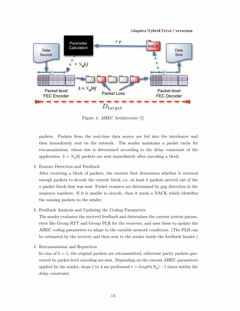
Figure 1: AHEC Architecture [1]
packets. Packets from the real-time data source are fed into the interleaver and
then immediately sent on the network. The sender maintains a packet cache for
retransmissions, whose size is determined according to the delay constraint of the
application. k +Np[0] packets are sent immediately after encoding a block.
2. Erasure Detection and Feedback
After receiving a block of packets, the receiver first determines whether it received
enough packets to decode the current block, i.e. at least k packets arrived out of the
n packet block that was sent. Packet erasures are determined by gap detection in the
sequence numbers. If it is unable to decode, then it sends a NACK which identifies
the missing packets to the sender.
3. Feedback Analysis and Updating the Coding Parameters
The sender evaluates the received feedback and determines the current system param-
eters like Group RTT and Group PLR for the receivers, and uses these to update the
AHEC coding parameters to adapt to the variable network conditions. (The PLR can
be estimated by the receiver and then sent to the sender inside the feedback header.)
4. Retransmission and Repetition
In case of k = 1, the original packets are retransmitted, otherwise parity packets gen-
erated by packet-level encoding are sent. Depending on the current AHEC parameters
applied by the sender, steps 1 to 4 are performed r = length(Np)−1 times within the
delay constraint.
14

The receiver feedback is used by the sender to analytically calculate the parameters
based on a statistical channel model in order to predict the reliability and the redundancy
produced by a certain coding parameter set. The parameter set that satisfies the application
constraints (target delivery time DTarget and reliability) with the lowest amount of redun-
dancy added is chosen. Therefore the receiver gets the quality of service it requires, at the
time it requires it in, assuming that channel capacity is sufficient. This will be an important
point for the use of bandwidth estimation techniques, as described in later chapters.
Table 1: Parameters of AHEC Scheme [13]
Symbol Definition
System Parameters
R Multimedia data rateL Packet lengthSimplified GE Packet loss modelRTT Round trip timePe Original link packet loss rateTs Packet interval
ConstraintsPLRtarget Packet loss rate requirement of applicationDtarget Delay constraint of application
Coding Parameters
Np Vector Np = (np,0, np,1, ..., np,r) defines the allocation of re-dundancy packets per round, where Np[0] = np,0 is the re-dundancy sent a priori with the original transmission andnp,i are the number of parity packets sent in the ith retrans-mission round.
k Number of data packets per block, i.e message lengthn Code word length
2.2 Analytical Design of Coding Parameters
Since the proposed protocol is supposed to adapt to the temporally changing network condi-
tions, we achieve adaptivity by analytical parameterization. Additional degrees of freedom
are available due to the combination of FEC and ARQ. Therefore, we can look at the
parameter search as an optimal distribution of the target delay budget by finding a good
trade-off between the number of retransmission rounds r = length(Np)− 1 and the coding
block length k. As presented by the authors in [1], we give a short description of the simple
analysis for the optimal coding parameters under the observed network state and the given
constraints for delay and residual error rate. The optimization target is - with minimum
redundancy RI - to guarantee a certain target packet loss rate (PLR) requirement under a
strict delay constraint.
By adjusting the block length k and number of retransmission rounds r = length(Np)−1,
15

according to the real-time stream’s average packet interval Ts and the observed round trip
time RTT , we can achieve a predictable and upper-bounded target coding delay DTarget.
For a chosen r we get,
k(r) =
⌊DTarget − (12 + r) ·RTT
Ts
⌋, (1)
where we have also included the transmission delay for the original transmission.
The authors of [18], apply the sequence analysis on the Gilbert-Elliot model, which repre-
sents a two state Markov chain, so as to estimate the residual erasure rate of a C(n, k) MDS
(Maximum Distance Separable) code, over a channel with erasure rate Pe and correlation
coefficient ρ for the state transitions. For a simplified analysis here, we choose the Gilbert -
Elliot model with zero correlation coefficient, equivalent to the binomial distribution. Then
the probability of d erasures in a sequence of n packets is given by,
Pdist(d, n) =(nd
)P de (1− Pe)
n−d. (2)
Let i denote the number of lost data packets in case of j packets being lost in one
encoding block of n packets. Since it is a systematic code, this means that amongst all of
the j lost packets in the block, there are i data packets lost from the k data packets and
there are j − i parity packets lost from n− k parity packets. Since all of the packets in one
encoding block have the same loss probability, the probability that j erasures in the block
of length n, hits i out of the k data packets is given by,
Pd(n, k, i, j) =
(ki
) (n−kj−i
)(nj
) . (3)
Then the residual loss rate of the C(n, k) code corresponds to the expected number of
unrecovered data packets per block divided by k,
Pres =1
k
k∑i=1
n−k+i∑j=max(n−k+1,i)
i · Pd(n, k, i, j) · Pdist(j, n). (4)
We choose a large enough n such that the residual erasure rate satisfies the PLR con-
straint and remains lower than PTarget.
16

The overall redundancy added on to the channel depends on the distribution of the
parity packets across the r retransmission cycles. By the wth round the number of packets
the sender has already sent are
−→n [w] = k +
w∑s=1
−→Np[s]. (5)
The retransmission round w is triggered by the loss notification in the previous round,
i.e. with the probability of decoding failure in the w − 1th round. Let Rw be the random
variable denoting the number of packets collected at the receiver at the end of the wth
round, then it is less than k with the probability,
Pr(Rw < k) =
−→n [w]∑j=−→n [w]−k+1
Pdist(j,−→n [w]). (6)
Then the overall redundancy is given by
RI =1
k
(−→Np[1] +
r∑w=2
Pr(Rw−1 < k).−→Np[w]
), (7)
where−→Np[1] is included because these parity packets are sent without receiver request.
The AHEC coding parameter set (k,−→Np) is iteratively adjusted between k and r, while
finding the optimal distribution of parity among the available retransmission rounds. Be-
sides just this naive long full search, a greedy algorithm to solve this optimization problem
also exists. Since this search of the optimal parameters is computationally quite intensive,
devices with limited processing capabilities should have pre-calculated tables of parameters
under typical scenarios, stored on them before hand.
2.3 PRRT Prototype Implementation
The prototype implementation of PRRT or Predictably Reliable Real-time Transport pro-
tocol suite is an enhanced version of the prevalent UDP stack to incorporate the above
described AHEC scheme that forms its core. In this thesis we will just give a brief outline,
for more details please refer to [12] and [13].
It is integrated as a kernel module into the Linux kernel, such that the AHEC function-
ality is encapsulated into a runtime-loadable kernel module. The inclusion of the prototype
1PRRT Project webpage : www.nt.uni-saarland.de/projects/prrt
17
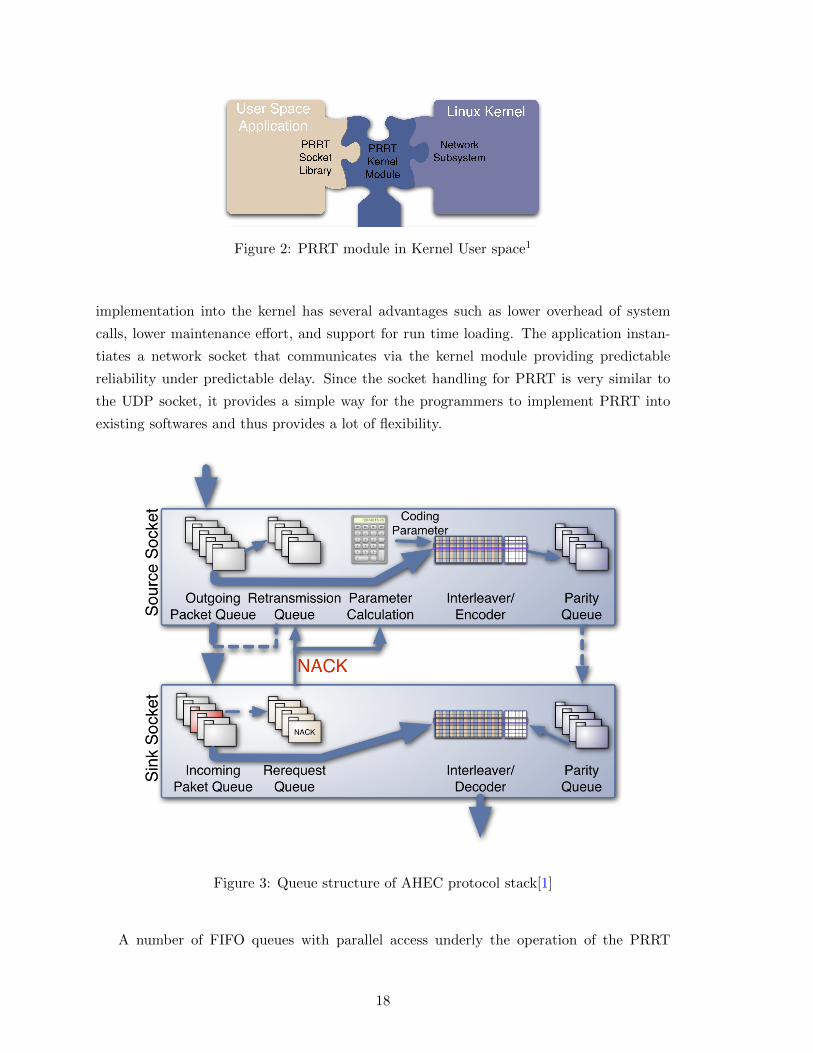
Figure 2: PRRT module in Kernel User space1
implementation into the kernel has several advantages such as lower overhead of system
calls, lower maintenance effort, and support for run time loading. The application instan-
tiates a network socket that communicates via the kernel module providing predictable
reliability under predictable delay. Since the socket handling for PRRT is very similar to
the UDP socket, it provides a simple way for the programmers to implement PRRT into
existing softwares and thus provides a lot of flexibility.
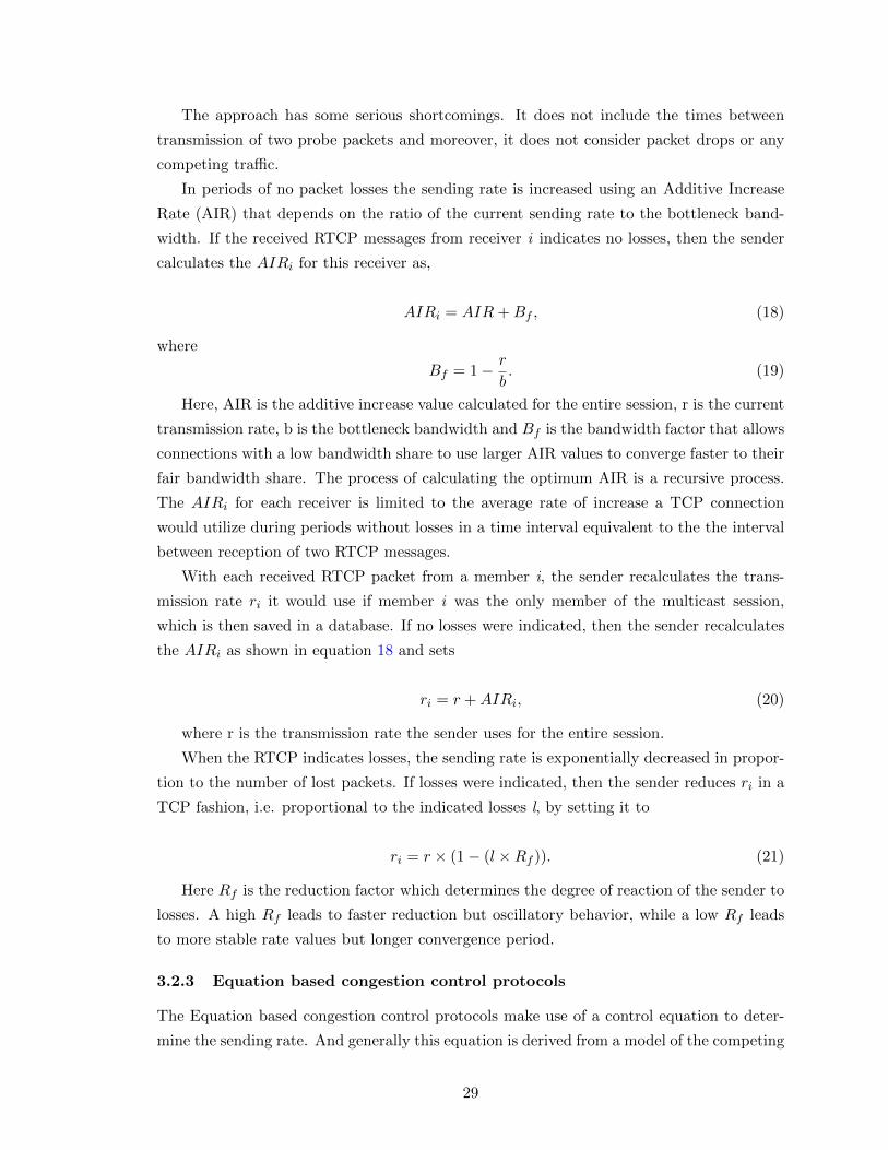
Figure 3: Queue structure of AHEC protocol stack[1]
A number of FIFO queues with parallel access underly the operation of the PRRT
18

protocol:
• Outgoing Packet Queue
Packets scheduled to be transmitted are put here. When they are put on to the
physical network to be transmitted the packets are also moved to retransmission
queue immediately.
• Retransmission Queue
The sender retains the transmitted packets in the retransmission queue to serve the
repetition requests for at least the target delay time.
• Incoming Packet Queue
At the receiver, gap detection, packet reordering and insertion of retransmitted packets
happens at the incoming packet queue. Also the parity packets are demultiplexed and
moved to parity queue.
• Re-request Queue
The information of the incomplete blocks from the gap detection is maintained in the
re-request queue. The feedbacks are sent periodically with the loss notifications.
• Parity Queue
Both the sender and the receiver maintain parity queues . At the sender, the packet
level encoder fills it and the retransmission requests are answered from the parity
queue. And at the receiver, the redundancy packets are supplied by the parity queue
to the packet level decoder.
The protocol stack provides a C/C++ socket library similar to the UDP socket API, to
make it more easy and familiar for the application programmers. The AHEC is configured
using socket options. The interface provides access to the channel state information and
the coding parameters, therefore an external application can perform parameter adaptation.
These coding parameters can either be obtained from pre-computed parameter tables, or
analytically as described in the previous section 2.2.
The prototype implementation inherits the multicast support and connectionless packet
delivery from the UDP stack.
2.4 Evaluation of AHEC Architecture under Limited Bandwidth
In the previous sections, we have introduced and elaborated on the media oriented PRRT
protocol and the AHEC mechanism that forms it’s core. It can be seen that there are a few
open issues in the current AHEC scheme. As of now, there is no upper limit to the amount
of redundancy that can be added to correct erasures. Therefore, in principle, we can correct
any error rate just because there is no upper limit to the amount of redundancy that can
19

be added. Also currently, the stream under consideration is assumed to be the only stream
and there is no mechanism to implement fairness amongst multiple simultaneous streams.
We address these issues of limited channel bandwidth and fairness towards other media
streams in this thesis.
Before discussing the solution for the functioning of AHEC under bandwidth constraint,
let us first evaluate how the AHEC architecture behaves under limited bandwidth.
2.4.1 Evaluation of Original AHEC Architecture
In the original formulation of the AHEC Architecture [18], the author had used Nrr which
gives the number of retransmission rounds and Nrt vector which defines the number of
redundancy packets retransmitted in one retransmission round for each lost packet, to
characterize the error correction mechanism. To satisfy the delay budget the trade off was
between the number of retransmission rounds and the coding block length. This could
therefore lead to a peak in the bandwidth requirement, because even though the elements
of the Nrt vector might be small individually, but they are still multiplied by the number
of NACKs received for a particular retransmission round. For example, if Nrr = 3, and
Nrt = {1, 1, 3} and 5 NACKs are received in the third retransmission round, then 5×3 = 15
packets would need to be retransmitted in a burst which would correspond to a peak in
the bandwidth requirement. Therefore even though this configuration could be sufficient to
reach some residual loss under certain network conditions, this came at the price of a very
large bandwidth requirement in the last retransmission round. This kind of bursty behavior
produced by redundancy transmissions was unwanted for the real time media applications.
2.4.2 Evaluation of Revised AHEC Architecture
In the revised architecture [1], the authors do not use the Nrt vector anymore, but instead
make use of the Np vector which defines how the n−k parity packets are distributed amongst
the different transmission rounds, where Np[0] gives the number of parity packets which are
sent a priori with the original transmission. Again in case any of the elements of the Np
vector become too large, then a burst of parity packets would be sent together and this can
lead to a bandwidth peak in the transmission. The queues on the routers do not distinguish
between the data packets and the parity packets, therefore with a sudden influx of large
number of parity packets, they may drop packets and there may even be congestion losses
due to queue overflows.
To exemplify this bursty behavior, we ran a short evaluation experiment over the
100Mbps network without any bottleneck bandwidth. Our sender and receiver were both
equipped with our PRRT protocol stack. We transmitted a high data rate stream from the
sender to the receiver, under the pure FEC configuration as well as the HEC configuration.
We then plotted the transmission bandwidth by using the throughput analysis feature of
20

the Wireshark1tool. The resulting plots of throughput against the transmission time are
shown in the diagrams 4 and 5.
Figure 4: Bandwidth peaks in throughput for pure FEC configuration
The plot shown in the diagram 4 shows the variation of the throughput along time for
a pure FEC case, with k = 50 and n = 80. As can be seen in the diagram, there are clear
bandwidth peaks in the throughput, and these are present throughout the transmission
time.
Figure 5: Bandwidth peaks in throughput for HEC configuration
1http://www.wireshark.org/
21

The plot shown in the diagram 5 shows the variation of the throughput along time for a
HEC case, with k = 50, n = 80 and parity packet distribution over the transmission rounds
given by Np = (5, 10, 15). Again it can be seen in the diagram that there are clear bandwidth
peaks in the throughput, and these are again present throughout the transmission time.
Therefore under a bottleneck bandwidth, these bandwidth peaks in the transmission
where longer bursts of parity are sent at once, can exceed the available bandwidth and lead
to congestion losses. Thus a pure FEC or a stronger HEC configuration is not possible
under bottleneck bandwidth in the current architecture.
22

CHAPTER III
BANDWIDTH ESTIMATION & CONGESTION CONTROL
Congestion occurs when the amount of data being transmitted through a network begins
to approach the data carrying capacity of the network. The objective of the congestion
control mechanisms is to maintain the amount of data in the network below the level at
which the performance drops off significantly. Consequently congestion control is a research
area where there has been extensive work in the past. In this chapter we will take a look
at the different classes of congestion control protocols and discuss their suitability for our
purpose of congestion control for media transmission.
For the multimedia transmission over a network, bandwidth is a key factor that affects
the packet loss rate. The packet loss rate may be severe if the sending rate is not adaptively
adjusted according to the network conditions, in turn, leading to congestion losses. There-
fore we will also take a look at the available techniques for bandwidth estimation, which as
stated, is closely related to the congestion control and adaptive rate adjustment.
3.1 Bandwidth Estimation Techniques
Knowing the bandwidth of the channel in an adaptive manner is crucial for ensuring that we
utilize the bandwidth using the most optimum codes, and without giving rise to congestion.
In the following sub-sections we present a brief overview of these bandwidth estimation
techniques for the purpose of congestion control and discuss their suitability for our pur-
pose of realtime media transmission.
Let us first take a quick look at the array of techniques available for estimating the
bandwidth on the channel. Though there can also be passive measurements [19] techniques
where we have a trace of the network conditions collected before hand. These are not of
interest to us, but we are interested in the active probing techniques. The typical active
probing techniques are packet pair/train dispersion (PPTD), variable packet size (VPS)
probing, Self-Loading Periodic streams (SLoPS) and Trains of Packet Pairs (TOPP).
3.1.1 Packet Pair/Train Dispersion (PPTD)
In packet pair probing technique [20], [21], the source sends multiple packet pairs to the
receiver. The receiver computes the end-to-end capacity by observing the delay between
the packets of the packet pairs, or in other words the dispersion which is experienced by
the packet pairs. Since the method is susceptible to the influence of cross traffic, therefore
23

a number of packet pairs are sent and filtering is done using statistical methods.
3.1.2 Variable Packet Size (VPS) probing
VPS probing [22], [23] measures the capacity of each hop along a transmission path. The
key element of the technique is to measure the RTT from the source to each hop of the path
as a function of the probing packet size. It sends multiple probing packets of a given size.
VPS makes use of the Time to Live (TTL) field of the IP header to force probing packets
to expire at a particular hop. The router at that hop then discards the probing packets,
and returns an ICMP “Time-exceeded” error message back to the source. The source uses
the received ICMP packets to measure the RTT to that hop. The RTTs for different packet
sizes are plotted, and the inverse of the slope of the graph gives the capacity of the link.
Unfortunately, the capacity estimates produced by VPS are often wrong. In the presence
of store-and-forward layer 2 devices like switches and hubs, they add extra transmission
latency and this leads to underestimation of the link capacity. Several tools like pathchar
[22], clink [28], and pchar [29] work on this principle.
3.1.3 Self-Loading Periodic streams (SLoPS)
In SLoPS [24], a sequence of packet probe trains is sent at a specific rate, where each of the
packet trains is of the same size. The sender tries to modify its sending rate such that it can
bring the stream rate close to the available bandwidth of the path. The sender varies its
sending rate by observing the variations in the one-way delays which are seen by the stream.
If the streaming rate is greater than the available bandwidth on the path, there will be a
short term overload in the bottleneck link’s queue, leading to an increase in the one way
delay of the probing packet trains. And inversely, when the streaming rate is less than the
available bandwidth, the one way delays of the packet train will not increase. Even though
SLoPS does overcome the inaccuracies in the existing probing techniques, it still can not
be used for real-time applications because it requires very large number of packet streams,
and also very long measurement periods. Pathload [27] is a tool based on this technique.
3.1.4 Trains of Packet Pairs (TOPP)
TOPP [25] sends many packet pairs at gradually increasing rates from the source to the
sink. This basic idea is very similar to SLoPS. In fact most of the differences between the
two methods are related to the statistical processing of the measurements. Also, TOPP
increases the offered rate linearly, while SLoPS uses a binary search to adjust the offered
rate. An important difference between TOPP and SLoPS is that TOPP can also estimate
the capacity of the tight link of the path. This capacity may be higher than the capacity
of the path, if the narrow and tight links are different. Here tight link refers to the link in
the path with the lowest available bandwidth, while the narrow link is the bottleneck link.
24

This methodology is not able to capture the fine grained interaction between the probes and
the competing flows and this temporal queuing behavior is useful for available bandwidth
estimation.
[30] provides a very comprehensive comparison study of the different bandwidth estima-
tion methodologies and tools.
3.2 Congestion Control Mechanisms
Next we take a look at the different kinds of congestion control mechanisms. They can
be broadly classified into three categories, the window based congestion control, TCP-like
congestion control protocols and the equation based congestion control mechanisms. We
will next describe each of these briefly, and give an example of each.
3.2.1 Window-based congestion control protocols
Window-based congestion control protocols, as the name suggests make use of a congestion
window just like TCP, and therefore portray a similar behavior. They vary the size of their
windows in order to regulate the amount of information being injected into the network,
based on the network conditions. TCP, in particular, makes use of Additive Increase, Multi-
plicative Decrease (AIMD) mechanism, such that it linearly increases the congestion window
size to probe the available bandwidth, and when it encounters congestion it decreases its
window size multiplicatively (by halving it).
3.2.1.1 LIAD for TCP Congestion Control
Here the TCP congestion control mechanism has been modified to fit the requirements of
heterogeneous wireless networks by making use of an adaptive window congestion control
mechanism, LIAD or Logarithmic Increase and Adaptive Decrease. The analysis of the
adaptive bandwidth prediction based LIAD for TCP congestion control scheme [6] is based
on the RTT. In the slow start phase, LIAD adopts the same exponential increase mechanism
with the available bandwidth prediction for determining the ideal slow start threshold. The
logarithmic increase takes place to increase the cwnd every time an ACK is received in
the congestion avoidance phase. And the adaptive decrease is based on an adaptive shrink
factor based on an adaptive bandwidth prediction. This is used to dynamically shrink the
cwnd in the congestion avoidance phase.
Figure 6 shows the transmission of data and acknowledgment segments in a TCP con-
nection, where S is the maximum segment size and R is the data rate of the connection. The
round trip time is RTTmin, when the network is not saturated. In a light traffic network,
the total time for sending a segment is therefore SR +RTTmin. And in a light traffic network,
25

Figure 6: Data and Acknowledgement transmission of a TCP connection [6]
increasing the cwnd does not increase the round trip time and the total time for sending
cwnd segments should be less than SR +RTTmin,
cwnd.(MSS
Rate) < (
MSS
Rate) +RTTmin. (8)
In the increasing cwnd phase, while the expected bandwidth is sufficient, the cwnd is
constrained by
cwnd <RTTmin
MSSRate
+ 1 (9)
which is derived by rearranging the terms of the inequality 8.
The optimal cwnd size is given by the right hand side of the inequality 9 .This is the cwnd
beyond which the network traffic is saturated, and the RTT progressively keeps increasing
till congestion occurs finally. In this expression, the RTTmin is the minimum RTT of the
connection when the network traffic is not yet saturated, MSS is the maximum segment
size and the Rate is the data rate of the connection.
The RTT is used as a measure of the traffic load in the network. The RTT value
based on the ACKs is used to determine the slow start threshold, ssthresh adaptively. The
ssthreshideal is given by
ssthreshideal =RTTmin
InterACK+ 1, (10)
which is basically the optimal cwnd for the current traffic load on the network. Here,
a modified - EWMA value of InterACK period is used as the parameter to represent the
26

current traffic load. Modified Exponentially Weighted Moving Average (M - EWMA) model
is used to compute the new expected smooth InterACK (InterACKnew) given by,
InterACKnew = α · InterACKcurrent + (1− α) · InterACKDiff, (11)
InterACKDiff = InterACKcurrent − InterACKold. (12)
Here, InterACKcurrent is the current inter-ACK time, InterACKDiff is the difference be-
tween the current and previous ACKs, and α is a constant value in the range (0,1). Thus
both in the case of a wireless link with non-consecutive packet loss (i.e. receiving non
consecutive duplicate ACKs), and in a wired network with consecutive loss of packets (i.e.
receiving consecutive duplicate ACKs), M-EWMA supports a fast response and thus has the
inherent capability to differentiate between these two types of packet losses (wired link’s
consecutive congestion losses and wireless link’s non-consecutive corruption losses) for a
better estimate of the available network bandwidth. The adaptive Network Bandwidth is
estimated using RTT of the last received ACK :
Adaptive Network Bandwidth =ssthreshideal
RTT. (13)
Under the estimated bandwidth, cwnd increases exponentially until the cwnd exceeds
the ssthreshnet in the slow start phase and then enters into the congestion avoidance phase.
ssthreshnet is given by
ssthreshnet = (Adaptive Network Bandwidth)×RTTmin (14)
= ssthreshideal ×RTTmin
RTT. (15)
This implies that ssthreshideal of the estimated network bandwidth occurs when the
RTT for the network is same as RTTmin. The term RTTminRTT is called the shrink factor of
the ssthreshideal. When the network becomes congested, the RTT increases and the shrink
factor decreases and the optimal cwnd shrinks. If the DUPACK is due to packet loss in a
wireless link, RTT is not affected and the shrink factor is not updated, therefore the cwnd
remains unchanged.
3.2.1.2 TCP Emulation at Receiver (TEAR)
Another approach in this category of window based congestion control protocols is TEAR
[5]. In this approach a congestion window is maintained and the sending rate is set using
the size of the congestion window. The congestion window or cwnd is located at the receiver
instead of being maintained at the sender to make the protocol suitable also for multicast,
in addition to unicast transmissions. Its size is manipulated similar to as is done for TCP,
27

by emulation of the timeouts and triple DUPACKs by the receiver. The RTT is measured
at the receiver, and the sending rate is maintained as cwnd/RTT .
3.2.2 TCP - like congestion control protocols
These congestion control protocols adjust their sending rate according to TCP’s Additive
Increase Multiplicative Decrease (AIMD) mechanism, but do not make use of a congestion
window.
3.2.2.1 Loss Delay based Adjustment Algorithm
Loss Delay based Adjustment Algorithm [8] is a TCP friendly adaptation scheme, in which
the transmission rate of the media applications adapts to the congestion level of the network
in a TCP friendly manner. It is a sender based adaptation scheme that relies on the
RTP/RTCP for feedback information about the losses and RTT. During periods without
losses, the sender increases its transmission rate by an Adaptive Increase Rate (AIR), which
is estimated using the loss, delay and bottleneck bandwidth values reported in the RTCP
feedback reports. During under load periods, the transmission rate is increased by AIR,
and it is multiplicatively decreased during congestion periods.
In RTP, each session member periodically sends RTCP reports to all other session mem-
bers. The sender reports contain the amount of data sent and the timestamp of when the
report was generated. The receiver report includes the fraction of lost data, timestamp of
last received sender report, tLSR, for a stream and the time elapsed between receiving last
sender report and sending the receiver report, tDLSR. The RTT can then be determined by
RTT = RRrecvd − tDLSR − tLSR. (16)
The propagation delay for the connection is taken as the minimum measured RTT.
The bottleneck of a network is estimated by enhancing RTP with the packet pair ap-
proach. The essential idea behind the approach is that if two packets can be caused to
travel together such that they are queued as a pair at the bottleneck, with no packets
intervening between them, then the inter-packet spacing will be proportional to the time
required for the bottleneck router to process the second packet of the pair. Therefore, a
stream of n packets is sent at the access speed of the end system. Then at the receiver site,
the bottleneck bandwidth is given by,
Bottleneck Bandwidth =probe packet size
gap between two probe packets. (17)
The data packets are used as the probe packets to avoid adding packets to the network
load.
28
The approach has some serious shortcomings. It does not include the times between
transmission of two probe packets and moreover, it does not consider packet drops or any
competing traffic.
In periods of no packet losses the sending rate is increased using an Additive Increase
Rate (AIR) that depends on the ratio of the current sending rate to the bottleneck band-
width. If the received RTCP messages from receiver i indicates no losses, then the sender
calculates the AIRi for this receiver as,
AIRi = AIR+Bf , (18)
where
Bf = 1− r
b. (19)
Here, AIR is the additive increase value calculated for the entire session, r is the current
transmission rate, b is the bottleneck bandwidth and Bf is the bandwidth factor that allows
connections with a low bandwidth share to use larger AIR values to converge faster to their
fair bandwidth share. The process of calculating the optimum AIR is a recursive process.
The AIRi for each receiver is limited to the average rate of increase a TCP connection
would utilize during periods without losses in a time interval equivalent to the the interval
between reception of two RTCP messages.
With each received RTCP packet from a member i, the sender recalculates the trans-
mission rate ri it would use if member i was the only member of the multicast session,
which is then saved in a database. If no losses were indicated, then the sender recalculates
the AIRi as shown in equation 18 and sets
ri = r +AIRi, (20)
where r is the transmission rate the sender uses for the entire session.
When the RTCP indicates losses, the sending rate is exponentially decreased in propor-
tion to the number of lost packets. If losses were indicated, then the sender reduces ri in a
TCP fashion, i.e. proportional to the indicated losses l, by setting it to
ri = r × (1− (l ×Rf )). (21)
Here Rf is the reduction factor which determines the degree of reaction of the sender to
losses. A high Rf leads to faster reduction but oscillatory behavior, while a low Rf leads
to more stable rate values but longer convergence period.
3.2.3 Equation based congestion control protocols
The Equation based congestion control protocols make use of a control equation to deter-
mine the sending rate. And generally this equation is derived from a model of the competing
29

traffic, for example TCP.
3.2.3.1 TCP Friendly Rate Control protocol
In TCP Friendly Rate Control protocol [2], the long term throughput equation of TCP
(Reno) is used as the control equation. The sender explicitly adjusts its sending rate as a
function of the measured rate of loss events in response to feedback from the receiver. The
loss event rate and RTT are fed to the control equation which governs the sending rate.
Therefore it performs similar to TCP’s AIMD mechanism.
3.2.3.2 Wave and Equation Based Rate Control
Wave and Equation Based Rate Control (WEBRC) [3] is an equation based multiple rate
multicast congestion control protocol. Being an equation based approach it ensures fairness
towards TCP with lesser fluctuations in the flow rate than TCP. It makes use of multicast
round trip time (MRTT) as a parameter to adjust the reception rate. MRTT is measured
independently by the receivers without any added burden on the sender, receiver or the
network. MRTT, similar to unicast RTT, increases with increasing queueing delay. It
synchronizes and equalizes the reception rates of the receivers in a proximity and causes
them to increase with the density of receivers.
A WEBRC sender transmits packets on a base channel and on T wave channels. The
transmission pattern on each wave channel is a sequence of periodically-spaced waves sep-
arated by quiescent periods. In a fluid model, the rate of each wave is predominantly
described by an exponential decay by a factor of P each T seconds. The beginnings of
the waves are designed so that the sum over all of the channels of the fluid-model rate is
constant. At any time the receiver is receiving from the base channel and some number
of other consecutive waves depending on the target reception rate of the receiver. The
receivers measure the loss event rate and MRTT and update their target reception rate.
WEBRC is mainly intended for applications for reliable download which can receive
packets from different channels.
3.3 Summary
As seen in the previous sections, an alternative to the window based congestion control
mechanisms are the rate based congestion control mechanisms, where the sending rate is
directly adjusted to the amount of congestion in the network. These are most useful for
applications like streaming multimedia, which are inherently rate based. In these cases
it is easier to modify the sending rate to conform to the timing, delay jitter or minimum
bandwidth constraints imposed by the application. It provides more flexibility than TCP
by decoupling reliability and congestion control.
30
As described in section 3.2.3.1, TCP Friendly Rate Control (TFRC) protocol is an
equation based congestion control scheme which has the TCP throughput equation as its
control equation ensuring TCP friendliness, in addition to the above mentioned advantages
of equation based approaches. Therefore TFRC is our chosen approach for congestion
control with bandwidth estimation. We give the details of the working of the TFRC protocol
in the next section.
3.4 TCP Friendly Rate Control (TFRC) Protocol
One of the aims of this thesis is to make our media oriented protocol suite TCP - friendly. As
mentioned earlier in section 1.1, fairness towards other competing protocols, specially TCP
is a big point of public concern. Non -TCP flows are considered TCP-friendly when their
long term throughput does not exceed the throughput of a TCP connection under the same
network conditions. Different TCP variants can achieve considerably varying throughputs.
The loss patterns also affect the TCP throughput, and therefore different TCP variants
respond differently to the same loss pattern. Therefore, a TCP-friendly flow’s sending rate
should be in the same order of magnitude as the corresponding TCP throughput under
the same network conditions, and not necessarily follow the throughput of a specific TCP
variant.
Now that we know what TCP friendliness is, we proceed on to describe how the TFRC
operates.
3.4.1 Loss Event Rate
The loss event rate p, is the key essence of the TFRC protocol. The loss event is defined
as one or more packets lost within one round trip time. Therefore subsequent losses, after
the first loss within a round trip time, are ignored. This means that at most there can
only be one loss event in one round trip time. Another term of importance is loss interval.
Loss interval is defined as the number of packets between loss events. Figure 7 shows the
relationship between the loss events and the loss intervals.
Loss event rate p is estimated as the inverse of the average loss interval, as described
later in section 3.4.4.
3.4.2 Model for TCP Throughput
For TCP friendly rate control, the appropriate choice for the control equation is the TCP
response function characterizing the steady state sending rate of TCP as a function of RTT
and the steady state loss event rate. (This does not accurately estimate the short-term
throughput during a single RTT, but average long-term throughput over multiple RTTs. )
31

Figure 7: An example of loss events and loss intervals
T =s
RTT√
2p3 + tRTO(3
√3p8 )p(1 + 32p2)
, (22)
is the TCP response function [2] [7] which gives the upper bound on the sending rate
T , as a function of the packet size s, RTT , steady state loss event rate p, and the TCP
retransmit time out value tRTO.
This model of the TCP throughput assumes that there is at most one window reduction
event per RTT. This TCP behavior is approximated by assuming that if a packet is lost in
a window, all the subsequent packets of the window are also lost.
This model is adjusted for TCP with selective acknowledgements (SACK - TCP). Since
SACK -TCP performs better than all other TCP variants in high loss states, therefore this
throughput model may overestimate the throughput of some of the TCP variants.
The loss event rate is measured at the receiver. The receiver either sends loss event rate
or the calculated transmission rate back to the sender, at least once per RTT. Every time a
feedback message is received, sender calculates the new value for the sending rate T, using
the control equation. If the actual sending rate is less than T, the sender may increase its
sending rate, otherwise it must decrease its sending rate to T.
For a multicast scenario it is more viable for the receiver to determine the relevant
parameters and calculate the allowed sending rate. In our implementation also the receiver
calculates the bandwidth estimate and sends it to the sender, as described in section 4.2.
32
3.4.3 Estimation of round-trip time and timeout value
The RTT can be measured at the sender as well as at the receiver. The timeout value, tRTO
is estimated as 4×RTT . This coarse estimation is justifiable because here, unlike in TCP,
it is only used as a parameter for the TCP model and not for scheduling the retransmissions
of packets. Therefore its impact on the sending rate is only noticeable at high loss rates.
3.4.4 Estimation of loss event rate
Most TCP implementations reduce their sending rate in response to a packet loss only once
per window. Further losses in the same window are ignored. Usually the losses are measured
as the loss fraction, which is just the ratio of the lost packets to the number of transmitted
packets. But the way TCP responds to losses is not modeled accurately by this loss fraction,
as TCP typically reduces the congestion window only once in response to several losses in
a window. A loss event therefore can consist of one or more packets lost within one RTT.
The definition of loss events complies with the one reduction event at maximum per RTT
by many TCP variants. To emulate the behavior of TCP conformant implementation, the
losses within an RTT that follow an initial loss are explicitly ignored and the protocol is
modeled such that it reduces its window at most once for a congestion notification in one
window of data. Therefore the losses are measured as the loss event fraction. If N packets
are transmitted in one RTT period, ploss is the packet loss probability, then the loss event
fraction is determined as,
Loss Event Fraction =Probability of losing at least 1 packet out of N
N(23)
=1− (1− ploss)N
N. (24)
Practically, we compute the loss event rate, indirectly by determining the average loss
interval, as described in the next section. Loss event rate is then the inverse of the average
loss interval.
3.4.4.1 Weighted Average Loss Interval Method
We measure the loss event rate over a certain interval of time, which is called the loss history.
The length of the measurement period provides a trade off between responsiveness by using
a short period, against stability by using a longer period. To measure the loss event rate
we use the indirect method of measuring the average loss interval, which is defined as the
average number of packets between loss events. The estimated loss event rate is the inverse
of the average loss interval.
The average loss interval method measures the arithmetic average loss event rate over
the last n loss intervals. Let si be the number of packets in the ith most recent loss interval,
33

and so be the interval containing the packets since the last loss event. so is the as yet non -
terminated loss interval and it must only be included in the average loss interval calculation
when it is large enough to increase the average loss interval value when included in this
calculation. The weighted average loss interval method takes a weighted average of the last
n loss intervals, with the average loss interval given by,
savg =
n∑i=1
wisi
n∑i=1
wi
(25)
Till the time the total number of loss intervals is less than n, the total number of loss
intervals are used to calculate the average loss interval. A weight distribution which is
best suited is such that it ensures that the recent loss intervals which represent the current
congestion state of the network have equal weights and the older intervals after a certain
number of intervals have smoothly decreasing weights so that the older loss events do not
affect the average loss interval estimate. For this reason, the weight of the n/2 most recent
intervals is set to one and the remaining n/2 have weights decreasing to 0.
wi = 1, 1 ≤ i ≤ n/2, (26)
= 1− i− n/2n/2 + 1
, n/2 < i ≤ n. (27)
Currently n=8 is chosen as it gives a good compromise between stability and responsive
as shown by the authors of TFRC [2]. Therefore we get the weights as w1, w2, w3, w4 = 1;
w5 = 0.8 ; w6 = 0.6; w7 = 0.4 and w8 = 0.2.
We also calculate the average loss interval including the as yet non terminated loss
interval, or so,
s′avg =
n−1∑i=0
wi+1si
n∑i=1
wi
(28)
and to ensure that so is only included at the right times as mentioned before, we use
the maximum of savg and s′avg as the estimate for the average loss interval.
3.4.4.2 History Discounting
To allow more timely response to sustained decrease in the congestion in the network,
history discounting is used to smoothly discount the weights given to older intervals when
a significantly long interval since the last loss event is encountered. When so is more than
34

twice the last estimate of average loss interval, the weights of older intervals are discounted
by the discount factor,
di = max(0.5,2savgso
), i > 0, (29)
do = 1. (30)
Therefore the estimated average loss interval is then,
s′avg =
n−1∑i=0
diwi+1si
n∑i=1
di−1wi
(31)
When loss occurs and so is shifted s1, then discount factors are also shifted such that if
a loss interval is ever discounted, then it is never un-discounted, and it’s discount factor is
never increased.
3.4.5 Bandwidth Estimation using TFRC
Now by observing the packet losses at the receiver, we can measure the loss event rate. This
packet loss history since the last feedback and the value of the RTT are are used to calculate
the bandwidth estimate for the network channel using equation 22. This estimate for the
channel bandwidth is fed back to the sender. The details of implementation of the TFRC
which is included within our media transport protocol PRRT, is given in section 4.2.
3.4.6 TCP Friendly Multicast Congestion Control (TFMCC) Protocol
A drawback of TFRC is that it is only meant for unicast environments. But with the
trend towards multicast and applications like multimedia streaming, which would benefit
from multicast, TFMCC [4] was developed which extends the functionality of TFRC to
multicast environment. The major problem with TFRC in multicast scenario is of feedback
implosion, where a large number of receivers would send feedback to the sender. Therefore
some changes need to be made. The target sending rate is computed at the receivers,
as the different receivers may experience different network conditions. Now the receiver
needs to measure the RTT between itself and the sender. Therefore the receivers send
packets to sender which echoes them including the timestamp for when it was sent. To
limit the feedback from the receivers to the sender, a feedback is sent only if the estimated
sending rate is less than the current actual rate. To ensure that there is some mechanism to
increase the sending rate, a receiver in the multicast group which seems to have the lowest
throughput is chosen as the ”Current Limiting Receiver” or CLR. It is allowed to send the
35

feedback immediately, and therefore the sender can increase or decrease the sending rate
appropriately. A new CLR needs to be chosen when another receiver’s throughput goes
below the throughput of CLR, or the CLR leaves the multicast group.
During a change in the network conditions when other receivers are affected, a CLR is
not of much help. Therefore in addition to the CLR, exponentially weighted randomized
timers are used, with a bias to favor feedback of the low-rate receivers, are used. When the
timer expires the receiver sends its calculated sending rate to the sender by unicast. If the
rate is lower than any of the feedback received previously, the sender forwards the sending
rate to all the receivers. The original technique of exponentially weighted randomized timers
is improved upon, as stated earlier, by biasing the feedback such that low rate receivers are
favored. Therefore when required a new CLR can be suitably selected, and all of it is done
while avoiding a feedback implosion.
TFMCC is designed to work with a multicast group consisting of thousands of receivers
and the authors have reported that TFMCC behaves similar to TFRC, with regards to
fairness towards TCP.
36

CHAPTER IV
PROPOSED SOLUTION FOR INCLUSION OF BANDWIDTH
LIMITATION
In this thesis, our aim is to estimate the bandwidth in the network, and incorporate this
bandwidth estimate with our analytical design of parameters so as to reduce or rather
control the congestion in the network. As we also described in section 1.1, the motivation
for this is two fold: firstly we want to reduce the bursts in the throughput introduced due to
packet correction in our AHEC scheme; and secondly, we want to provide fairness to other
protocols. To address the short comings of the current AHEC scheme and to provide fairness
towards other streams, an adaptive bandwidth estimation is proposed to be included in the
analysis and the PRRT stack for the media transmission.
In the next section 4.1, we describe analytically how we make use of the bandwidth
estimation to control the congestion in the network, and its inclusion in our parameter
analysis. Following that, in section 4.2, we give the proposed architecture details of our
solution for the bandwidth estimation and its incorporation in our PRRT stack.
4.1 Analytical Solution for Optimizing under Limited Bandwidth
In section 2.2, we have presented a simple analysis for the optimal coding parameters.
The optimization target there was to guarantee a certain target packet loss rate (PLR)
requirement under a strict delay constraint, and to do so with minimum redundancy, RI.
Therefore if we look closely there is already an inherent bandwidth limitation integrated
into the AHEC parameter analysis in the form of the redundancy information that can be
added, and this redundancy is kept to a minimum under the other two constraints of target
delay and residual packet loss rate.
With the estimate of the bandwidth in the network, we can basically have two different
modes of operation. We could either transmit the media stream as it is and the bandwidth
estimation could just determine whether error correction is feasible or not, with the resid-
ual loss rate varying accordingly. Or otherwise, we could adapt the source rate to some
bandwidth constraint with enough headroom to allow the amount of redundancy required
to meet a reliability constraint under a fixed amount of delay.
In the rest of the section we discuss these two options and their implications. We discuss
their feasibility for our parameter analysis and thus justify our choice of the second option
as our chosen mode of operation.
37
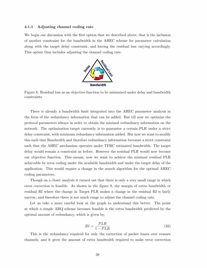
4.1.1 Adjusting channel coding rate
We begin our discussion with the first option that we described above, that is the inclusion
of another constraint for the bandwidth in the AHEC scheme for parameter calculation
along with the target delay constraint, and having the residual loss varying accordingly.
This option thus includes adjusting the channel coding rate.
Figure 8: Residual loss as an objective function to be minimized under delay and bandwidthconstraints
There is already a bandwidth limit integrated into the AHEC parameter analysis in
the form of the redundancy information that can be added. But till now we optimize the
protocol parameters always in order to obtain the minimal redundancy information on the
network. The optimization target currently is to guarantee a certain PLR under a strict
delay constraint, with minimum redundancy information added. But now we want to modify
this such that Bandwidth and therefore redundancy information becomes a strict constraint
such that the AHEC mechanism operates under TFRC estimated bandwidth. The target
delay would remain a constraint as before. However the residual PLR would now become
our objective function. This means, now we want to achieve the minimal residual PLR
achievable by error coding under the available bandwidth and under the target delay of the
application. This would require a change in the search algorithm for the optimal AHEC
coding parameters.
Though on a closer analysis it turned out that there is only a very small range in which
error correction is feasible. As shown in the figure 9, the margin of extra bandwidth or
residual RI where the change in Target PLR makes a change in the residual RI is fairly
narrow, and therefore there is not much range to adjust the channel coding rate.
Let us take a more careful look at the graph to understand this better. The point
at which a simple ARQ scheme becomes feasible is the extra bandwidth predicted by the
optimal amount of redundancy, which is given by,
RI =PLR
1− PLR(32)
This is the redundancy required for only the correction of packet losses over erasure
channels, and it gives the amount of extra bandwidth required to make error correction
38

Table 2: Optimum Parameter Sets for different values of Target Packet Loss Rate
PTarget RIRes Kopt Npopt1.0e-1 0.00523008003017575 148 0,11.0e-2 0.00523008003017575 148 0,11.0e-3 0.00995942137082703 79 0,1,1,11.0e-4 0.0100000000000000 1 0,11.0e-5 0.0101000000000000 1 0,1,11.0e-6 0.0101010000000000 1 0,1,1,11.0e-7 0.0101010000000000 1 0,1,1,11.0e-8 0.0101010000000000 1 0,1,1,11.0e-9 0.0101010100000001 1 0,1,1,1,11.0e-10 0.0101010101000001 1 0,1,1,1,1,11.0e-15 0.0101010103000001 1 0,1,1,1,1,31.0e-20 0.0101010106000001 1 0,1,1,1,1,61.0e-25 0.0101010108000001 1 0,1,1,1,1,81.0e-30 0.0101010111000002 1 0,1,1,1,1,111.0e-35 0.0101010113000002 1 0,1,1,1,1,131.0e-40 0.0101010116000002 1 0,1,1,1,1,16
Figure 9: Bandwidth (Residual RI) vs Reliability (Target PLR)
feasible. Before this, when the bandwidth or residual RI is fairly low, it may be a scenario
such that we can only have a few parity packets with very long blocks of data providing
39

very low error correction capabilities and in such cases FEC may not even be feasible. This
phenomenon can be clearly seen in table 3.
After this point, the residual RI becomes almost constant such that even when you drop
the target PLR from 10−5 to 10−40t there is not much change in the residual RI or the
extra bandwidth requirement.
Therefore when we make the residual PLR our objective function that we want to mini-
mize under a certain bandwidth constraint, we see that just changing the bottleneck band-
width in an extremely narrow range already drastically drops the residual PLR, rendering
this option useless for our purpose.
4.1.2 Adjusting source coding rate
We now take a deeper look at the second and our chosen option. Here we adjust the source
coding rate according to the bandwidth estimate in order to avoid congestion while still
providing optimum error correction capabilities.
In our current analytical design of the coding parameters, our objective function is to
minimize the coding overhead, or the amount of redundancy. This redundancy is the extra
bandwidth being utilized on top of the bandwidth occupied by the data packets being sent
at the source coding rate.
To be media friendly, our scheme has to ensure that the media stream is not stalled at
any time. We adapt the source coding rate such that we leave enough head room for the
coding overhead.
Therefore we vary the source coding rate as,
SR ≤ BWest
(1 +RI)(33)
where, SR is the modulated source coding rate, BWest is the estimated bandwidth, and
RI is the coding overhead or the redundancy added. Therefore our bandwidth estimate
becomes one of the indirect parameters in our analytical error correction parameter calcu-
lation. Here RI is determined analytically by adjusting the channel coding rate, as shown
in section 2.2. And we adapt our source coding rate according to our bandwidth estimate.
This gives the tradeoff introduced between the source coding rate and the channel coding
rate. And hence in this combined source and channel coding scheme, the estimated band-
width determines the maximum source coding rate under a certain reliability and delay
constraints.
Therefore as described, we can really analytically determine the source coding rate. This
adaptation of the source coding rate according to the bandwidth estimate is quite different
from the other available protocols.
We can explicitly provide this source coding rate adaptation for media transmission
according to our bandwidth estimate and according to our analytical model for reliability,
40

to achieve a certain residual loss rate (which means, with predictable reliability). This
tradeoff introduced between the source coding rate and the channel coding, in order to
achieve a certain reliability is not provided by the other available schemes. We either have
fixed or full reliability as in the case of TCP, or non-deterministic amount of reliability as
in the case of DCCP - PR, with a certain source coding rate. But this kind of analytical
adjustment between the two of them is not available there.
To put it differently, in our scheme we would be able to increase the source coding rate
or the perceptual quality of the video, at the expense of more artifacts in a certain amount
of time, or increase the reliability at the cost of more source coding artifacts in the form of
lower quality of coded images. Thus there is an adjustment between the losses, resolution
and hence the quality of experience.
4.2 Proposed Architecture for Bandwidth Estimation using TFRC
After describing our proposed solution analytically in the previous section, and showing how
it fits with our analytical design of the coding parameters, we now proceed to describing
our proposed architecture of the congestion control solution using bandwidth estimation.
As mentioned in the previous section, this basic idea of bandwidth adaptation method by
adjusting the source rate at the PRRT sender in our transport paradigm is quite a new one.
To begin with, we consider the scenario where we have one sender and one receiver with
a bottleneck router in between them. Both the sender and the receiver are equipped with
the PRRT stack which has been enhanced with our bandwidth estimation using TFRC to
provide a congestion control scheme in a TCP friendly manner.
Currently our solution is limited to offer bandwidth estimation for unicast scenario with
one sender and one receiver. Even though the extension to multicast scenario is left for
the future, we give an intuition and possible solution for our algorithm in the multicast
scenarios at every step.
Before going into the depth of the functionalities of the sender and the receivers for the
purpose of our bandwidth estimation using TFRC, lets us first enumerate the parameters
we require for it:
• Round Trip Time : In case of a multicast scenario, we need to have an estimate
of the group round trip time, GRTT. And we need to ensure that this estimate of
the GRTT leads to an underestimation of the bandwidth as compared to the actual
situation at each of the single receivers. This is ensured because we account for
the worst possible receiver in the receiver group and therefore the GRTT basically
represents the worst case RTT. But in the current case we consider a single receiver,
and the extension to multiple receivers is left to future work.
• Retransmit Time-out Interval : This is an input to the TCP throughput equation
41

(22). As mentioned in section 3.4.3, it is estimated as 4 times the RTT value.
• Minimum Packet Interval : This is the minimum packet interval observed at the
receiver, and is used to estimate the bandwidth in the initialization slow start phase
of our algorithm, as explained later in this section.
• Loss Map : The receiver also generates a loss map, which is basically the loss pattern
observed at the receiver representing which packets were received and which ones were
lost. The details of its generation are also given later in this section.
• Average Loss Interval : The average loss interval is required to estimate the average
loss event rate, which is given as the reciprocal of the average loss interval as shown
by the authors in [7]. The loss interval, as mentioned earlier also, is the number of
packets in between two loss events.
Figure 10: Functionalities of the sender and receiver in bandwidth estimation
As shown in figure 10, the sender estimates the group round trip time, and sends it
to the receiver. The receiver does an exponentially weighted moving average of the RTT
samples received to feed into the TCP throughput equation, given by equation 22 for the
purpose of bandwidth estimation. At the receiver, the loss map is also generated which
facilitates the computation of loss event rate. The minimum packet interval observed at the
receiver is made use of for the initialization of the bandwidth estimation. Making use of
all these parameters, the receiver estimates the bandwidth and this estimated bandwidth
is sent to the sender. The sender takes the estimated bandwidth reported back by the
42

receiver, and uses it to modulate the sending rate of the sender in such a manner, so as to
control the congestion in the underlying network. All these boxes shown in the figure are
the functionalities added to the PRRT protocol stack to function under limited bandwidth
while controlling the congestion in the network.
We will now elaborate on these functionalities of the sender and the receiver in the next
sections.
4.2.1 Sender Functionalities
As we can see from the figure 10, two main functions are performed at the sender side: the
RTT estimation and the modulation of sending rate. This in turn may include rate limiting
by traffic shaping at the sender. We will now delve into both of these in more detail.
4.2.1.1 RTT Measurement
Let us first see how RTT is measured in PRRT in the general case. In each packet the
sender sends, it also includes a time-stamp TSsent which denotes when the packet was sent.
At the receiver’s side, before it sends a feedback it selects the sender’s time-stamp Tsent
from the most recently received packet from the sender. It then adds to it the time elapsed
between receiving this packet and sending the feedback, Telapsed, and sends it back to the
sender. The sender receives this feedback at time Treceived.
Figure 11: Measurement of Round Trip Time
43

As evident from the figure 11, the RTT can be determined as
RTT = Treceived − (Tsent + Telapsed) (34)
The advantage of this method for determining the RTT is that it requires no synchro-
nization between the sender and the receiver clocks.
To work in a multicast scenario, the group RTT is measured at the sender, and then
broadcasted to all the receivers in each packet. In our current implementation of the protocol
RTT is computed at the sender and fed to the receivers in each data packet. This is essential
for the proper functioning of PRRT because the protocol decisions like the timeouts for the
different retransmission rounds and synchronization is dependent on this measure of the
group RTT. In the conservative approach to adapt to the worst receiver in the multicast
group, the RTT is determined for this worst receiver and used as the group RTT. Though
currently, we are using just a moving average of all the received RTT samples at the sender.
4.2.1.2 Modulating the Sending Rate
The estimated bandwidth sent in the feed back by the receiver to the sender, is used to
modulate the sending rate of the sender. Maintaining the sending rate at the right level is
essential so as to not lead to a congested state of the network.
The closed loop feedback inherent in this sender-receiver scheme leads to fluctuations
in the estimated bandwidth at the receiver. When the sending rate is much lower than the
bottleneck bandwidth and there are no losses, then the receiver sends a higher estimate.
When the sending rate is naively increased to this estimate, this may lead to more and
more traffic in the network, finally leading to a congested state, where the queues at the
bottleneck router are full. In this case RTT increases, and since packets may be dropped,
therefore the loss event rate also increases. Consequently the TFRC estimates a lower
throughput using the TCP throughput equation. This lower estimate is then sent to the
sender and it tries to now reduce the sending rate. To avoid this closed loop behavior and
the oscillations, we must not naively increase the sending rate to the estimated bandwidth,
but we must adapt slowly to this estimate. Instead of increasing the sending rate slowly at
the sender, we slowly increase the bandwidth estimate at the receiver, therefore sending a
more gradually varying bandwidth estimate to the sender to counter this effect of the closed
loop behavior. This is explained in more detail when we discuss the receiver functionalities
in section 4.2.2.
Also since this sending rate is the data rate of the data packets being sent, therefore
we need to leave some head-room for the redundancy which is added on top of these data
packets, in the form of the parity or redundancy packets. Therefore we need to reduce the
sending rate by an equivalent amount to be able to accommodate all the redundancy also.
44

And to improve the bandwidth estimate we should include the loss of parity packets in the
loss map for the calculation of the loss event rate.
Another aspect that we need to deal with due to the added redundancy is the bursty
nature of these parity packets. The parity packets tend to be sent all at once in a short
burst. Due to these bandwidth peaks congestion may develop in the network. To avoid
this we need to smoothen out the packet sending rate in time, such that there are no such
bursts.
We tried to make use of a token bucket approach to rate limit the sender, and to
smoothen out the sending rate to avoid the bandwidth peaks in transmission as reported
during the evaluation of the AHEC scheme under limited bandwidth, in section 2.4. It is a
popular algorithm for traffic shaping or rate limiting, and works by controlling the amount
of data that is sent on the network channel, though it still allows for bursts of data to be
sent.
In a token bucket 1approach, the traffic can only be transmitted if there are enough
tokens in the bucket. The bucket of size b contains tokens of fixed size, and these are used
up for the ability to send corresponding amounts of data. If the token rate is r, then every
updation interval of s seconds, s × r tokens are added to the bucket. The bucket can at
maximum hold b tokens, and if a token arrives while the bucket is full then it is discarded.
Over a long period of time, the sending rate of the packets is limited by the token rate
r. The estimated available bandwidth gives the upper limit to the possible sending rate,
therefore it is used to limit the token filling rate.
If m is the maximum possible transmission rate, then the maximum burst size for which
the maximum possible rate m is fully utilized if given by,
Lmax =
b×m(m−r) , if r < m
∞, otherwise(35)
where, Lmax is the maximum burst size, b is the token bucket size, and r is the token
filling rate. Therefore if configured properly, a flow can transmit up to its peak burst rate,
if there are enough tokens in the bucket.
NETEM provides a token bucket filter(TBF) which can be used to smoothen out the
sending rate. It could be configured with a rate twice the bottleneck bandwidth of the
router, and a buffer size equivalent to that of the routers. The details of the NETEM and
the TBF it provides are given in the next chapter in section 5.1.
Though in our current implementation we do not make use of the token bucket filter as
it was observed that it is not able to sufficiently space out the parity packets temporally.
1http : //en.wikipedia.org/wiki/Token bucket
45

Figure 12: Token Bucket Filter2
This spacing out will have to be included into the AHEC protocol stack, and this is not as
yet implemented. We discuss this further in the results and observations section 5.2.
4.2.2 Receiver Functionalities
We now proceed on to discuss the functionalities of the receiver. As can be seen from figure
10, the receiver contains all the functionality for the estimation of the bandwidth with
just group RTT being reported by the sender. The functions that the receiver performs
can be broken into two main subtasks: loss event rate measurement and then bandwidth
estimation. In the following sections we describe how both of these subtasks are done at
the receiver.
4.2.2.1 Loss Event Rate Measurement
As mentioned in section 3.4, the loss event rate is the main loss indicator in the TFRC
protocol. Therefore a good estimation of the loss event rate is essential for the performance
of the protocol and for our bandwidth estimation. Therefore we make use of the average
loss interval estimation method with history discounting to make sure that the bandwidth
2http://tldp.org/HOWTO/Traffic-Control-HOWTO/classless-qdiscs.html
46
estimation does react to drastic changes in the network conditions, while still providing a
stable sending rate.
The loss event rate, to be fed into the TCP response equation (22) which gives the
upper bound on the steady state TCP throughput, is estimated at the receiver. This is
specially beneficial for the multicast scenario, where each receiver just uses the loss event
rate experienced locally to estimate the bandwidth and sends only the bandwidth estimate
to the sender. It is better than to have the sender maintain loss event information for each
receiver, as that would have been an added overhead for the sender.
To be able to calculate the loss event rate, the receiver needs the loss pattern which is
basically a map of what all packets were received and which ones were lost. At the receiver
the loss map is maintained with a pointer that keeps track of the last packet that arrived.
By looking at the sequence numbers of the arriving packets, gap detection or the detection
of intermediate missing packets is possible. As and when a packet arrives, the pointer is
advanced that many positions ahead according to it’s sequence number, while marking the
intermediate positions on the map corresponding to the lost packets as 1. For the packets
which are received the corresponding positions in the loss map are marked as 0.
Every round trip time, the receivers calculate the loss event rate based on the loss pattern
observed in the last round trip time period. The receiver uses this loss pattern to populate
the loss history for the weighted average loss interval method as described in section 3.4.4.1,
to determine the average loss interval. The loss interval history is maintained as a circular
buffer, with pointers for the oldest and the most recent intervals. The history discounting
is also implemented to ensure the correct functioning as described in the earlier chapter.
As described in the aforementioned section, the loss event rate is estimated as the inverse
of the average loss interval length.
4.2.2.2 Estimating the Bandwidth
With the loss event rate and the RTT estimates in place, we will now talk about the
estimation of the bandwidth at the receiver.
To begin with, initially in the cases where the packet loss rate is almost zero, or where
there are almost no losses, the TCP response equation used in TFRC estimates a very high
value for the throughput. To counteract this, we make use of the minimum packet interval
observed at the receiver. Using this minimum packet interval and the packet size, we can
estimate the bottleneck bandwidth,
Bottleneck Bandwidth =packet size
minimum packet interval(36)
47

Figure 13: Bottleneck Bandwidth Estimation
Therefore to initialize our bandwidth estimate for our protocol, we make use of this
estimate like in the slow start phase of the TCP congestion control, till we encounter the
first loss, when we shift to estimating the bandwidth using the TCP throughput equation.
One inherent problem of loss based congestion control approaches is that it uses packet
losses to limit the sending rate. Thus TFRC increases the rate till any packet losses happen,
and therefore in a situation where there are no other competing flows, it ends up filling up
the queue of the bottleneck router. Though of course the queues are being filled up in the
case of multiple competing streams too.
Figure 14: Transition from Slow Start to Normal Operation Phase
In the cases when there are losses we make use of the TCP throughput equation to
estimate the bandwidth. This control equation has to be fed with the loss event rate and
48
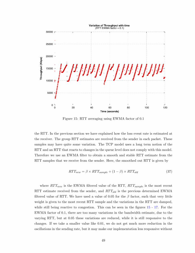
Figure 15: RTT averaging using EWMA factor of 0.1
the RTT. In the previous section we have explained how the loss event rate is estimated at
the receiver. The group RTT estimates are received from the sender in each packet. These
samples may have quite some variation. The TCP model uses a long term notion of the
RTT and an RTT that reacts to changes in the queue level does not comply with this model.
Therefore we use an EWMA filter to obtain a smooth and stable RTT estimate from the
RTT samples that we receive from the sender. Here, the smoothed out RTT is given by
RTTnew = β ×RTTsample + (1− β)×RTTold (37)
where RTTnew is the EWMA filtered value of the RTT, RTTsample is the most recent
RTT estimate received from the sender, and RTTold is the previous determined EWMA
filtered value of RTT. We have used a value of 0.05 for the β factor, such that very little
weight is given to the most recent RTT sample and the variations in the RTT are damped,
while still being reactive to congestion. This can be seen in the figures 15 - 17. For the
EWMA factor of 0.1, there are too many variations in the bandwidth estimate, due to the
varying RTT, but at 0.05 these variations are reduced, while it is still responsive to the
changes. If we take a smaller value like 0.01, we do not get much more reduction in the
oscillations in the sending rate, but it may make our implementation less responsive without
49

Figure 16: RTT averaging using EWMA factor of 0.05
Figure 17: RTT averaging using EWMA factor of 0.01
50
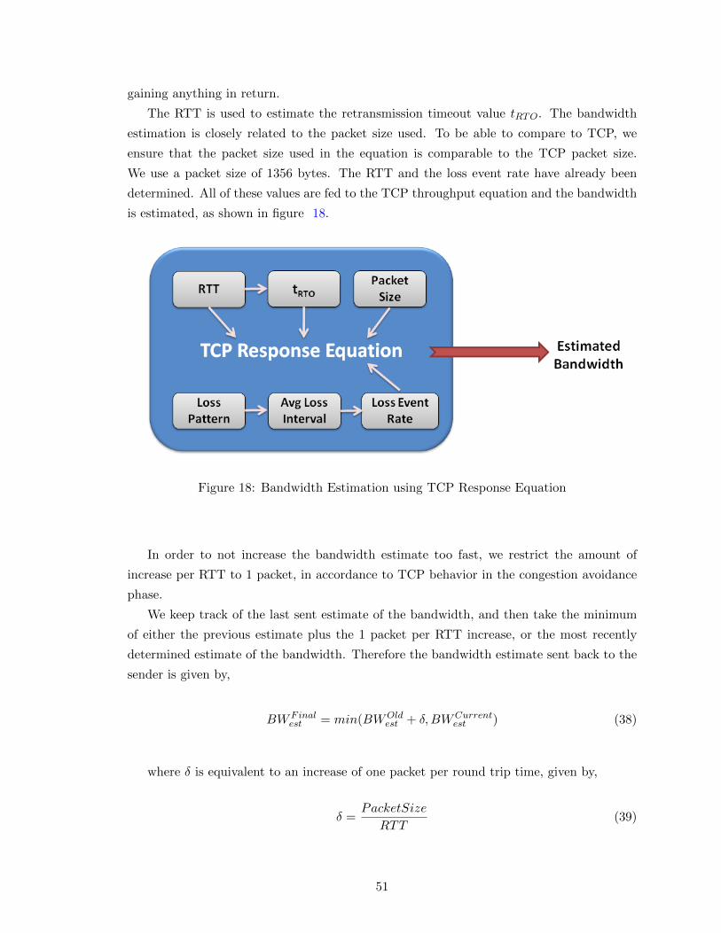
gaining anything in return.
The RTT is used to estimate the retransmission timeout value tRTO. The bandwidth
estimation is closely related to the packet size used. To be able to compare to TCP, we
ensure that the packet size used in the equation is comparable to the TCP packet size.
We use a packet size of 1356 bytes. The RTT and the loss event rate have already been
determined. All of these values are fed to the TCP throughput equation and the bandwidth
is estimated, as shown in figure 18.
Figure 18: Bandwidth Estimation using TCP Response Equation
In order to not increase the bandwidth estimate too fast, we restrict the amount of
increase per RTT to 1 packet, in accordance to TCP behavior in the congestion avoidance
phase.
We keep track of the last sent estimate of the bandwidth, and then take the minimum
of either the previous estimate plus the 1 packet per RTT increase, or the most recently
determined estimate of the bandwidth. Therefore the bandwidth estimate sent back to the
sender is given by,
BWFinalest = min(BWOld
est + δ,BWCurrentest ) (38)
where δ is equivalent to an increase of one packet per round trip time, given by,
δ =PacketSize
RTT(39)
51

This final estimated bandwidth BWFinalest is then sent back to the sender in the feedback
from the receiver.
4.3 Implementation Details
Figure 19: Sender Functionality
In this section we give some of the implementation details of our solution extending
TFRC for bandwidth estimation for the purpose of congestion control. The functionalities
of the the sender and the receiver have been elaborated in the previous section. We begin
by presenting a flowchart diagram for both the sender and the receiver, which portrays their
detailed functioning and we then go on to give more implementation specific details for each
of them.
4.3.1 Sender Implementation
The sender listens for feedback from the receiver. On getting the feedback from the receiver,
the sender estimates the RTT as explained in section 4.2.1.1. The Sender then inserts the
RTT estimate in each of the packets and sets it’s data rate to the bandwidth estimate
sent by the receiver. It then continues to send the data packets at the rate specified by
52

the receiver, interspersed with bursts of parity packets, till a new bandwidth estimate is
received from the receiver, as shown in figure 19.
4.3.2 Receiver Implementation
The receiver, in our implementation, does most of the work for bandwidth estimation. The
majority of the functionality is implemented at the receiver to keep the design scalable for
multicast.
The receiver has two phases of operation, the slow start phase and the normal operation
phase. Before any losses are encountered, and the loss interval history is initialized, the
receiver is in the slow start phase, and thereafter shifts to the normal operation phase.
In the slow start phase the receiver makes use of the minimum packet interval observed
to estimate the bandwidth and in the normal operation phase it makes use of the TFRC
mechanism and its control equation giving the steady state TCP throughput.
The receiver implementation has two main functions, one for calculating the bandwidth
estimate, calc T(), and the another one to calculate the average loss interval, calc avg loss interval().
Next we briefly describe the functioning of both of these functions.
calc T
Initialization : Phase = SlowStart
1. Obtain EWMA filtered value of RTT,
RTT = 0.05 ∗RTT + 0.95 ∗RTTPrev
RTTPrev = RTT
2. Calculate Bottleneck BW
bnBW = PktSize ∗ 8/minPktInterval
3. Check if there are no losses in the loss map generated and current phase is Slow Start
Phase
if yes
then Slow Start Phase, go to 4
else
Normal Operation Phase, go to 5
4. Slow Start Phase
Multiply the bnBW by the slow start factor (currently set to 2 , same as TCP) and
return this to sender as bandwidth estimate.
Go back to 1
53

5. Calculate retransmit timeout as
tRTO = 4 ∗RTT
6. Calculate Avg Loss Interval
7. Determine Loss event rate as the reciprocal of avg loss interval
8. Calculate the throughput, using TFRC’s control equation 22
Feed in the RTT, tRTO and loss event rate to get BW Est
9. Store the throughput value as BWprev
10. Calculate increase of 1 pkt per RTT
δ = PktSize ∗ 8/RTT
11. Determine receiver’s BW estimate as
min ( BW Est , BWprev + δ)
12. Send final BW Est to Sender
13. Wait for observation period of time, then go back to 1
Next we describe the function calc avg loss interval(), which makes use of two ring
buffers for loss interval history and the history discounting weights. Each of them has two
pointers, one pointing to the most recently added element and one for the oldest element
in the buffer. These two pointers are manipulated appropriately to keep account of the the
two histories as described in sections 3.4.4 and 4.2.2.1.
calc avg loss interval()
1. Iterate through the loss map and keep incrementing the current loss interval s0 in the
history till the first lost packet is encountered
2. This is a loss event and beginning of a new loss interval.
Shift the loss interval into the loss history to s1 and start counting for the most recent
loss interval s0, and make corresponding changes in the history discounting ring buffer.
3. If the current loss interval s0 is more than twice the previously estimated average loss
interval, then enable new history discounting weights for it
di = max(0.5,2savgso
), i > 0,
do = 1.
and
s′avg =
n−1∑i=0
diwi+1si
n∑i=1
di−1wi
54

4. Calculate the average s avg 1 using loss interval history and history discounting, with-
out including the current loss interval s0
savg =
n∑i=1
wisi
n∑i=1
wi
5. Calculate the average s avg 0 using loss interval history and history discounting, in-
cluding the current loss interval s0
s′avg =
n−1∑i=0
wi+1si
n∑i=1
wi
6. avg loss interval = max(s avg 0, s avg 1)
For more details, the reader is requested to take a look at the code listings.
55
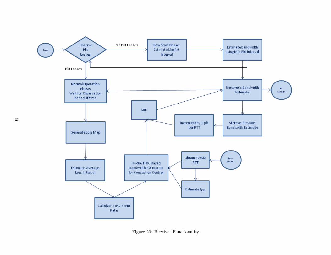
Figure 20: Receiver Functionality
56

CHAPTER V
EVALUATION
5.1 Experimental Setup
Our experimental setup basically consists of a sender and a receiver connected via a router
as shown in figure 21. Both the sender and receiver are equipped with the PRRT stack
along with our solution for congestion control by estimating the bandwidth. We emulate
the network conditions using Netem.
Figure 21: Experimental Setup
We use static routes, and have implemented the router using Netem and a token bucket
filter. Netem is a module of Linux kernel that provides Network Emulation functionality for
testing protocols by emulating the properties of wide area networks. The current version of
Netem emulates variable delay, loss, duplication and re-ordering.
Now we present the step by step procedure to set up the router and have the sender
and receiver communicating via the router, for our experiments.
1. Firstly we configure the sender and receiver with static ip addresses by assigning their
ethernet interfaces an ip address from different subnets using ifconfig as shown below.
i f c o n f i g eth0 1 9 2 . 1 6 8 . 0 . 2
i f c o n f i g eth0 1 9 2 . 1 6 8 . 1 . 2
57

Here, for example, 192.168.0.2 is the ip address of the sender and 192.168.1.2 is the
ip address of the receiver.
2. Next we configure the router by assigning the gateway ip addresses to its ethernet
interfaces.
i f c o n f i g eth0 1 9 2 . 1 6 8 . 0 . 1
i f c o n f i g eth1 1 9 2 . 1 6 8 . 1 . 1
3. Then we enable static routing by assigning the static routes using the gateways, as
shown below.
echo 1 | sudo tee −a / proc / sys / net / ipv4 / ip fo rward
route add −net 1 9 2 . 1 6 8 . 0 . 0 gw 1 9 2 . 1 6 8 . 1 . 1 netmask 2 5 5 . 2 5 5 . 2 5 5 . 0 dev eth0
route add −net 1 9 2 . 1 6 8 . 1 . 0 gw 1 9 2 . 1 6 8 . 0 . 1 netmask 2 5 5 . 2 5 5 . 2 5 5 . 0 dev eth1
4. Finally we add the bottleneck at the router by doing rate limiting using token bucket
filter (TBF) to limit the output, as Netem has no built-in rate control.
tc qd i s c add dev eth1 parent 1 : 1 handle 10 : tb f r a t e 15000 kb i t b u f f e r
3000 l i m i t 6000
tc qd i s c add dev eth1 root handle 1 : 0 netem delay 0ms
In the above case, we use a bottleneck rate of 15000 kbits, with a buffer of 3000 bytes
and a limit of 6000 bytes and no added delay.
5. Finally, at the sender and receiver we add the one way delays using Netem such that
we have our desired round trip time.
tc qd i s c add dev eth0 root netem delay Xms
If we configure both the sender and the receiver with this delay of Xms, then the
round trip would be approximately 2Xms.
One thing to note here is that we have created the bottleneck link by using Netem’s
token bucket filter for rate limiting at the outgoing ethernet interface towards the receiver.
This bottleneck link is shown as the link highlighted in red in the figure. This bottle-
neck bandwidth would then be observed by the receiver, as shown in the figure below and
depending on it the receiver would estimate the bandwidth.
58

Figure 22: Experimental Setup with the bottleneck at the router
5.2 Results & Observations
Congestion in the Internet is not a new phenomenon. It has always been there, maybe
even more due to the aggressive file streaming applications in the past rather than the
current burst of the media streaming applications. But as pointed out earlier, real-time
media streaming applications allocate a certain average, though limited, bandwidth due to
their encoding rate. Thus they have certain minimum bandwidth requirements even though
they may not saturate the channel. The remaining challenge now is to make sure that such
real-time media transmission applications interact in ”friendly and fair” manner with the
available internet services.
In this section we present the results of our work. We also discuss the reasons behind
some of the anomalies present in the results, as well as the weaknesses of the current
implementation. The aim of our thesis is to include the bandwidth limit into our AHEC
architecture for error correction and to modify the PRRT protocol stack to include it while
maintaining friendliness towards other protocols. As explained in the previous chapters, we
have adapted TFRC for our purpose of real time media transmission and this is integrated
with our AHEC scheme for the purpose of congestion control using bandwidth estimation.
For all of our experiments described next, we set the bottleneck bandwidth at the router
as 15000Kbps, with a round trip time of 30ms between the sender and the receiver. No
additional packet loss rate is emulated. The sender is configured for error correction with
number of data packets per coding block, k=1, retransmission rounds given by vector Np
= {0,1,1,8}, and target delay, Dtarget = 200ms, unless specified otherwise.
The loss event rate is the primary indicator of congestion in the TFRC mechanism, and
consequently in ours too. The loss event rate is estimated as the inverse of average loss
interval, which is defined as the number of packets between loss events. Please recall that
59
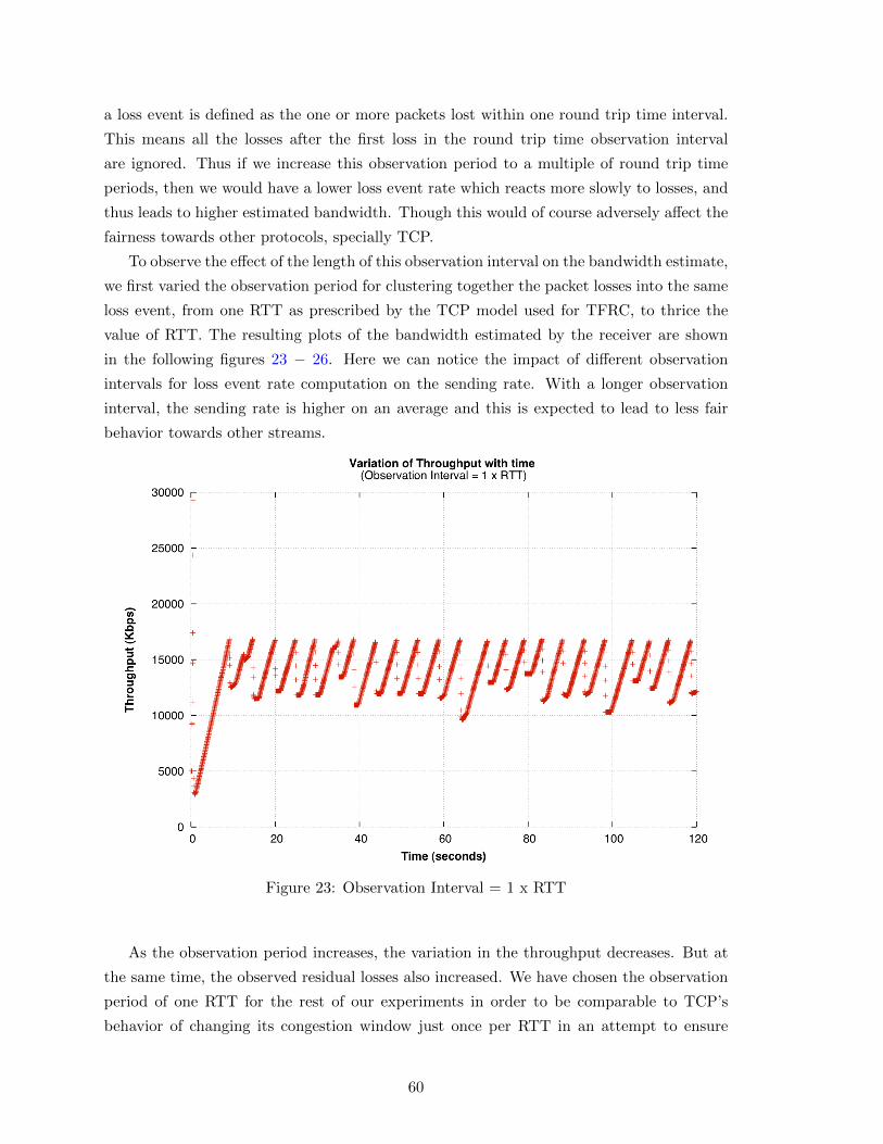
a loss event is defined as the one or more packets lost within one round trip time interval.
This means all the losses after the first loss in the round trip time observation interval
are ignored. Thus if we increase this observation period to a multiple of round trip time
periods, then we would have a lower loss event rate which reacts more slowly to losses, and
thus leads to higher estimated bandwidth. Though this would of course adversely affect the
fairness towards other protocols, specially TCP.
To observe the effect of the length of this observation interval on the bandwidth estimate,
we first varied the observation period for clustering together the packet losses into the same
loss event, from one RTT as prescribed by the TCP model used for TFRC, to thrice the
value of RTT. The resulting plots of the bandwidth estimated by the receiver are shown
in the following figures 23 − 26. Here we can notice the impact of different observation
intervals for loss event rate computation on the sending rate. With a longer observation
interval, the sending rate is higher on an average and this is expected to lead to less fair
behavior towards other streams.
Figure 23: Observation Interval = 1 x RTT
As the observation period increases, the variation in the throughput decreases. But at
the same time, the observed residual losses also increased. We have chosen the observation
period of one RTT for the rest of our experiments in order to be comparable to TCP’s
behavior of changing its congestion window just once per RTT in an attempt to ensure
60
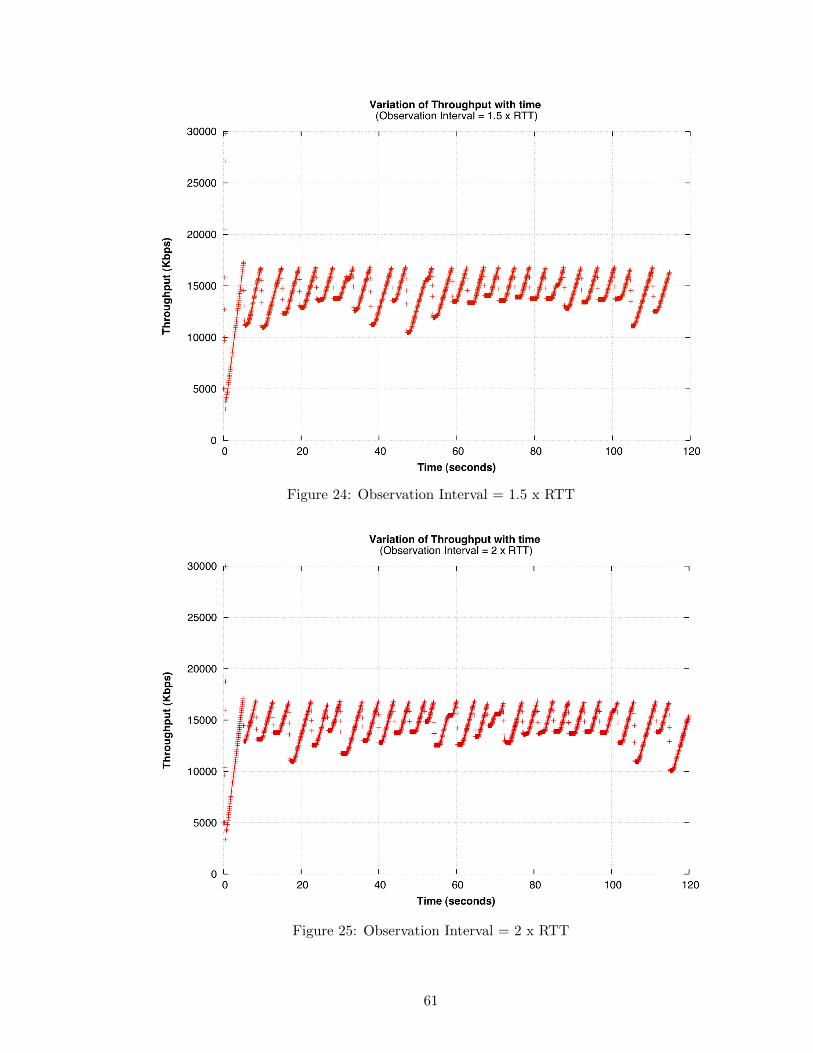
Figure 24: Observation Interval = 1.5 x RTT
Figure 25: Observation Interval = 2 x RTT
61

Figure 26: Observation Interval = 3 x RTT
TCP friendliness.
We can see in figure 23 that the throughput varies around the bottleneck bandwidth of
15000Kbps, even though there is an overestimation of the bandwidth at the receiver. The
reasons for this over estimation and the oscillations in the sending rate are two fold. Firstly,
in our loss map generation we do not as yet include the losses of the redundancy packets.
And secondly, the losses of the data and the redundancy packets are both overcome by
retransmissions in our AHEC scheme due to the ARQ mechanism kicking in. Therefore
at those instances the actual sending rate including the redundancy packets is in reality
a multiple of the bandwidth estimated by the receiver. And this, in fact, leads to more
congestion in the network and potentially to more congestion losses. To understand this
better, lets take a look at figure 27.
There is a slight overestimation of the bandwidth at the receiver due to the inaccurate
loss map lacking the loss information about redundancy packets. This results in an un-
derestimation of loss even rate, and thus the sending rate does not get reduced enough at
the right times. And on top of it the retransmissions lead to higher actual sending rate
as described above, and worsen the situation. This can be seen clearly in figure 27. The
oscillations in the sending rate have less amplitude in the case of error correction without
retransmissions. But in case of retransmissions for error correction, the drop in the sending
62

(a) With Retrnsmissions
(b) Without Retransmissions
Figure 27: Impact of retransmissions for error correction on sending rate
63

rate is more severe, potentially due to the bursty retransmissions of redundancy packets. In
this experiment we have used an error correction configuration with one data packet packet
per coding block with 11.8% redundancy information. Therefore the redundancy packets
not included in the bandwidth estimation computation can have a significant impact, as
also demonstrated in the figure.
At the instances when there are packet losses, the ARQ mechanism kicks in and there are
retransmissions as described earlier. This is an inherent short coming of the AHEC scheme
because as soon as we have these retransmissions the bandwidth increases significantly for
a short period of time, leading to congested network and potentially more losses. To avoid
this we need to temporally space out these redundancy packets, and this is not incorporated
in the AHEC scheme for media transmission as yet. This temporal spacing of redundancy
packets needs to be included into the analytical model itself to be able to get rid of these
bandwidth peaks and to ensure that the network does not get congested by modulating the
source coding rate according to the actual estimated bandwidth.
Finally we now take a look at the behavior of our bandwidth estimation solution for
congestion control in the presence of other competing traffic. TCP being the most prevalent
protocol on Internet, is specially of interest to us in order to show fairness towards the
protocols. In the following experiments we have generated TCP streams using iperf 1, and
transmitted them concurrently with our own stream of PRRT. The TCP streams are flowing
in the same direction as ours, i.e. from the sender to receiver across the bottleneck link as
shown in figure 28.
To observe the fairness of our protocol, lets take a look at the plots for the variation in
the sending rate in the presence of competing TCP streams. We can see that the average
sending rate in each case behaves quite fairly to the other streams, the sending rate being
approximately equal to the bottleneck bandwidth divided by the total number of streams
in the network. This is shown in the table 3 also, where the first column gives the number
of concurrent TCP streams flowing along with our PRRT stream. the second column gives
the bandwidth estimated by iperf for each TCP stream. The third column specifies the
average long term throughput of our PRRT stream, while the last column gives the fair
share of the bottleneck bandwidth according to the total number of streams sharing it.
A TCP friendly flow is defined as a flow whose sending rate is in the same order of
magnitude as the corresponding TCP throughput under the same network conditions as
described in section 3.4 . In table 3, we can see that the bandwidth estimated by iperf TCP
tests is of the same order of magnitude as our PRRT stream. There is an underestimation
of bandwidth by the iperf in case of very few TCP streams, as in that case the TCP streams
generated by it are not able to attain the bottleneck bandwidth due to the limited queue
size at our router implementation. Nevertheless, the bandwidth estimated by iperf’s TCP
1http://iperf.sourceforge.net/
64

Figure 28: Experimental Setup with concurrent TCP streams
Table 3: Estimated Bandwidth: Comparison of results
Num of TCPStreams
iperf estimated bandwidthper TCP stream (Kbps)
Avg throughputof PRRT Stream (Kbps)
Bottleneck Bandwidth/num of streams (Kbps)
1 2784 7733.06 75002 2719 5465.80 50005 2083 3453.74 250010 1278 1635.36 1363.6315 931 854.00 937.5
streams is of the same order of magnitude as ours and we have a reasonably TCP friendly
solution.
Therefore we have shown in this section the behavior of our bandwidth estimation
solution for congestion control of real time media transmission and also we have discussed
some of the shortcomings of our current implementation and their effect on the results. In
section 7.2, we summarize the missing features of our current implementation and give hints
about how to overcome the current deficiencies.
65
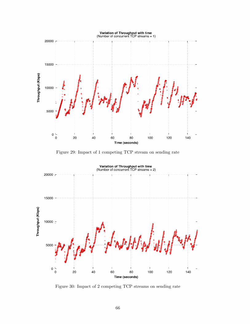
Figure 29: Impact of 1 competing TCP stream on sending rate
Figure 30: Impact of 2 competing TCP streams on sending rate
66
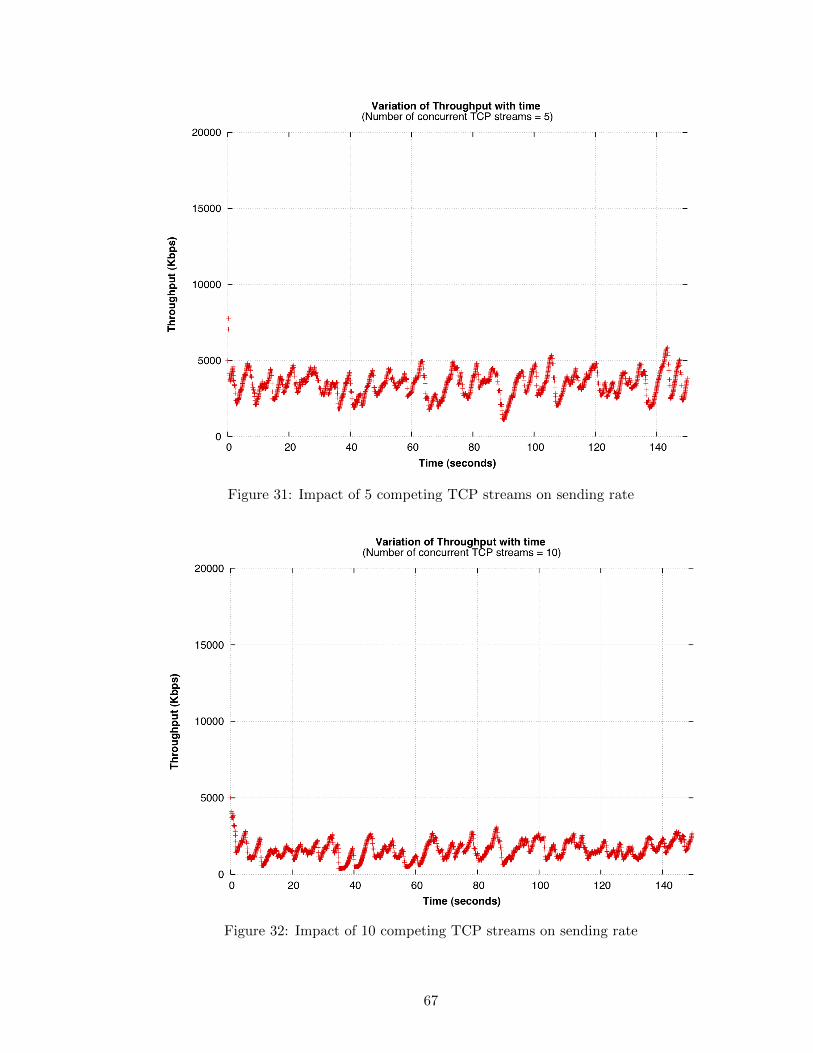
Figure 31: Impact of 5 competing TCP streams on sending rate
Figure 32: Impact of 10 competing TCP streams on sending rate
67
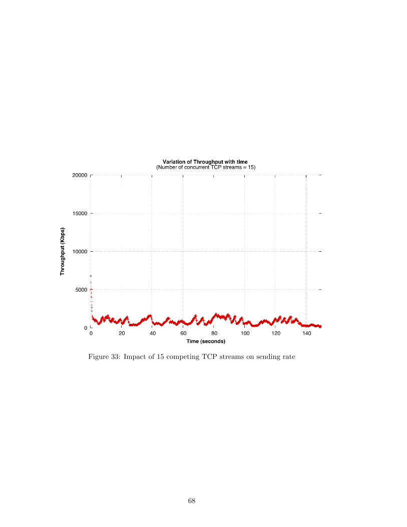
Figure 33: Impact of 15 competing TCP streams on sending rate
68

CHAPTER VI
DIFFERENTIATING CONGESTION AND CORRUPTION LOSSES
6.1 Need for loss differentiation
With the advent of wireless heterogeneous networks, a number of weaknesses of the current
transport layer protocols, specifically standard TCP, have become evident. One of the
shortcomings of the current transport layer protocols including TCP is that their congestion
control mechanism interprets all the losses as congestion losses due to overflowing queues at
the routers in the congested network. This is true even for other transport layer protocols
besides TCP, like SCTP and TFRC, where the packet losses are used as an indicator of
congestion in the network. This assumption leads to suboptimal performance due to the
transport layer’s inability to derive the reason for the packet being dropped. This is even
more incorrect in situations where we have wireless links in the network path, where a non
negligible percentage of packets are corrupted due to wireless corruption losses, and are
eventually dropped to ensure reliability. Therefore the performance is hampered by the
needless reduction of the sending rate due to the non-existent but perceived congestion,
which is in reality just packets being dropped due to corruption.
Therefore if we can differentiate between losses due to congestion and corruption then
we can react accordingly in our congestion control protocol. For instance, when the losses
are truly due to congestion, we should reduce our sending rate to reduce the number of
packets in the network, such that the queues at the router can come out of the overflowing
state. But on the other hand, in case of purely corruption losses it does not make sense to
reduce the sending rate. We should, in fact, retransmit the lost data and maybe even apply
stronger error correction techniques for reliable transport.
Besides this advantage of avoiding unnecessary reduction of sending rate, the differen-
tiation of losses can also be used to give useful feedback to the video encoder. Therefore, if
the encoder knows that there are a lot of wireless losses, then it can better balance its bits
between the source coding which represent the video and the channel coding which protect
the source coded bits.
In the next section, we discuss briefly the different techniques for improving TCP be-
havior in wireless lossy environments, and in the final section, we give a hint about how
we can integrate this loss differentiation information with our congestion control mecha-
nism in our media transport protocol. The actual implementation and inclusion of the loss
differentiation into the PRRT stack is left as future work.
69

6.2 Available Loss Differentiation Techniques
There are a fairly large variety of loss differentiation algorithms and techniques for improving
TCP performance available today, specially with the advent of the wireless heterogeneous
networks. Preventing TCP from reacting to wireless losses as if they indicated congestion
is an active area of research. In this section we give just a very brief introduction to some
of the broad types.
To avoid the degradation of performance of TCP due to all losses being interpreted as
congestion losses, several schemes have been proposed to improve the TCP performance
in lossy wireless environments. The authors of [33] have classified them broadly into 3
categories. The first one is the end-to-end protocols, where loss recovery is performed by the
sender by the use of selective acknowledgements (SACK) such that the sender can recover
from multiple packet losses in a window without having to resort to timeouts. Additionally,
it enables the sender to differentiate between losses by explicit loss notification (ELN)
mechanism. The second category is split connection protocols that break the end-to end
connection into two parts at the base station. The performance can be improved by the
use of negative or selective acknowledgements on the wireless link between the base station
and the end host . And the last ones are the link-layer protocols based on a combination
of ARQ and FEC techniques such that the wireless losses are hidden from the sender via
retransmissions and forward error correction. [9] is an example of the last type.
There has also been work on evaluating and improving TFRC for wireless networks. In
[14], the authors have presented an enhanced TFRC (E-TFRC) which incorporates a two
phase loss differentiation algorithm (TP-LDA) to detect and identify the cause of packet loss
events. The ratio of congestion losses to link losses is estimated by a cross layer approach
and this ratio is used to modify the loss event rate.
One final technique that we mention here is [34], where the authors have combined
TFRC with FEC. They apply FEC dynamically in only those instances when they detect
potential periods of increased TCP-induced congestion, such that the overhead generated in
form of redundant parity packets in FEC is used judiciously and kept to a minimum. They
observe the delay samples (Round Trip Time and Forward Trip Time) and their derivatives
and based on the clustering of loss events over the {RTT, ˙RTT} or {FTT, ˙FTT}, they
propose a dynamic FEC whose code rate is computed on the fly based on the instantaneous
values of these delays and their derivatives.
6.3 Integration with our solution - A Hint
Thus for a more efficient congestion control mechanism in today’s heterogeneous networks,
we need to differentiate between congestion and corruption losses. It’s inclusion in our con-
gestion control mechanism as an input to the loss rate calculation can help us to determine
the true loss rate due to congestion in the network, and lead to better and more optimal
70
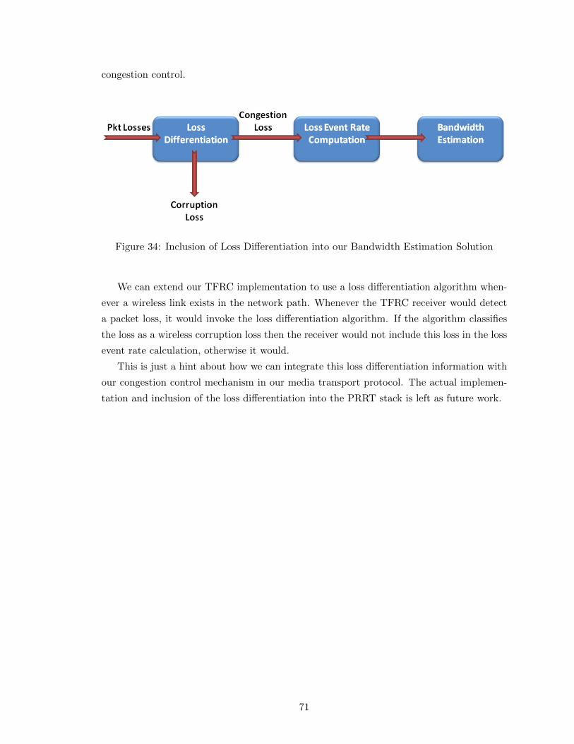
congestion control.
Figure 34: Inclusion of Loss Differentiation into our Bandwidth Estimation Solution
We can extend our TFRC implementation to use a loss differentiation algorithm when-
ever a wireless link exists in the network path. Whenever the TFRC receiver would detect
a packet loss, it would invoke the loss differentiation algorithm. If the algorithm classifies
the loss as a wireless corruption loss then the receiver would not include this loss in the loss
event rate calculation, otherwise it would.
This is just a hint about how we can integrate this loss differentiation information with
our congestion control mechanism in our media transport protocol. The actual implemen-
tation and inclusion of the loss differentiation into the PRRT stack is left as future work.
71

72

CHAPTER VII
CONCLUSION AND OUTLOOK
7.1 Summary
In this thesis we have used bandwidth estimation for the purpose of congestion control for
real-time media transmission. We have estimated the bandwidth using an adaptation of
the TFRC protocol.
We studied various methodologies for bandwidth estimation and congestion control and
found the equation based approach of TFRC to be favorable for inclusion into our AHEC
error correction scheme.
We considered two different scenarios for the inclusion of this bandwidth limit in our
AHEC scheme. The first option was to include bandwidth limit as a strict constraint in the
AHEC parameter analysis along with the target delay constraint and to treat the residual
packet loss rate as the objective function. But this approach of changing the channel
coding rate according to the bandwidth available in the network was later discarded as it
was discovered that the range in which the extra bandwidth for redundancy can be varied
is very narrow to be of much practical use. The second option was to change the source
coding rate according to the estimated bandwidth in the network. We chose this option of
changing the source coding rate according to the bandwidth estimated at the receiver. The
sender uses this estimated bandwidth to modulate its sending rate. The bandwidth limit is
inherently a part of the AHEC parameter analysis by the virtue of redundancy information
which is minimized under the target delay and packet loss rate constraints. The redundancy
information represents the extra bandwidth on top of the source data rate which is utilized.
We have implemented TFRC to estimate the bandwidth and integrated it with the
PRRT protocol stack’s implementation to provide real time media transmission in a con-
gestion controlled manner, along with error correction capabilities. Our protocol is fair
towards other streams and behaves in a TCP friendly way.
7.2 Future Work
In our current implementation, we have considered a unicast scenario, though our approach
can be extended to the multicast case. The basic difference would come in the RTT mea-
surement and feedback suppression. We can use the longest RTT as the limiting case. Or
the RTT estimation at the sender can be done by using a multicast tree approach such that
all the parent nodes know the RTT to their child nodes, and the total RTT along a path can
be the sum of the RTTs along the path. Also instead of sending a feedback immediately we
73

can have the receiver back off by sometime, and send the feedback only if no other receiver
has already sent back a lower estimated bandwidth. This would be a conservative approach
where we adapt to the worst conditions. In such a case we can have some entry check where
only those receivers are allowed to join the multicast groups which satisfy certain minimum
requirements.
For wireless scenarios, if a loss differentiation algorithm is used to differentiate between
the congestion and wireless corruption losses, then this information can be fed into our
solution to account for this distinction, such that the sending rate is reduced only in the
case of congestion losses and not corruption losses.
And finally, we need to take into account the losses of redundancy packets, which is
missing right now in our loss maps. We should include their loss information in the loss
map. Also we need to modify the current analysis in such a manner so as to temporally
space out the retransmissions and not send them in a bursty way. This is as yet lacking in
the AHEC parameter analysis.
74

REFERENCES
[1] M. Gorius, J. Miroll, M. Karl, T. Herfet, “Predictable Reliability and Packet Loss
Domain Separation for IP Media Delivery”, IEEE International Conference on Com-
munications (ICC), June 2011.
[2] S. Floyd, M. Handley, J. Padhye, J. Widmer, ”Equation-Based Congestion Control for
Unicast Applications: the Extended Version”, TR-00-003, March 2000.
[3] M. Luby, V. K. Goyal, S. Skaria, G. B. Horn,“Wave and equation based rate control
using multicast round trip time”, ACM SIGCOMM , 2002.
[4] J. Widmer, M. Handley , “TCP-friendly multicast congestion control (TFMCC): Pro-
tocol specification”, RFC 4654, August 2006.
[5] I. Rhee, V. Ozdemir, Y. Yi,“TEAR: TCP emulation at receivers - flow control for
multimedia streaming”, Technical Report, 2000.
[6] B. Chang, S. Lin, J. Jin, ”LIAD: Adaptive bandwidth prediction based Logarithmic
Increase Adaptive Decrease for TCP congestion control in heterogeneous wireless net-
works ”, May 2009.
[7] J. Padhye, V. Firoiu, D. Towsley, J. Kurose, ”Modeling TCP Throughput: A Simple
Model and its Empirical Validation”, May 1998
[8] D. Sisalem, H. Schulzrinne, ”The Loss-Delay Based Adjustment Algorithm: A TCP-
Friendly Adaptation Scheme”, Sisalem, 1998.
[9] F. Sun, V. O. K. Li, S. C. Liew, “Clustered-loss Retransmission Protocol over Wireless
TCP”, IEEE PIMRC, 2005.
[10] M. Gorius, M. Karl, T. Herfet, ”Optimized Link-level Error Correction for Internet
Media Transmission”, NEM Summit, 2009
[11] R. Gogolok, ”Optimization of an Application Layer Hybrid Error Correction Scheme
under Strict Delay Constraint”, Master Thesis, 2008
[12] J. Gruen, ”Design and Implementation of a Media oriented Network Protocol Stack”,
Diploma Thesis, 2009
[13] Future Media Internet : Video & Audio Transport - A New Paradigm, Manuscript,
Telecommunications Lab, University of Saarland, 2010.
75
[14] S. Pack, X. Shen, J. W. Mark, L. Cai,“A Two-Phase Loss Differentiation Algorithm
for Improving TFRC Performance in IEEE 802.11 WLANs”, IEEE Transactions on
Wireless Communications, 2007.
[15] Cisco and/or its affiliates, “Cisco visual networking index: Forecast and methodology,
2009-2014”, 2010.
[16] European Commission: Future Media Internet,
ftp://ftp.cordis.europa.eu/pub/fp7/ict/docs/netmedia/20080101-fimen.pdf.
[17] International Telecommunications Union: ITU-T Recommendation Y.1541, “Network
Performance Objecties for IP-based Services”, 2006.
[18] G. Tan, “Optimum Hybrid Error Correction Scheme under Strict Delay Constraints”,
Dissertation, 2008.
[19] J. C. Hoe, “Improving the Start-up Behavior of a Congestion Control Scheme for TCP”
, SIGCOMM, 1996.
[20] P. Ramanathan, C. Dovrolis, D. Moore, “What do Packet Dispersion Techniques Mea-
sure?”, INFOCOM, January 2001.
[21] R. L. Carter, M. E. Crovella, “Measuring Bottleneck Link Speed in Packet-Switched
Networks”, Perform. Eval.,1996.
[22] V. Jacobson, “Pathchar: A tool to Infer Characteristics of Internet Paths.”,
ftp://ftp.ee.lbl.gov/pathchar/, April 1997.
[23] S. Bellovin,“A Best-Case Network Performance Model.”, Technical Report, ATT Re-
search, Feb. 1992.
[24] M. Jain, C. Dovrolis, “End-to-End Available Bandwidth: Measurement Methodology,
Dynamics, and Relation with TCP Throughput.”, IEEE ACM Trans. Netw., 2003.
[25] B. Melander, M. Bjorkman, P. Gunningberg, “A New End-to-End Probing and Anal-
ysis Method for Estimating Bandwidth Bottlenecks.”, GLOBECOM O00. IEEE, 2000.
[26] G. Tan, T. Herfet, “Evaluation of the Performance of a Hybrid Error Correction Scheme
for DVB Services over IEEE 802.11a”, IEEE International Symposium on Broadband
Multimedia Systems and Broadcasting (ISBMSB),March 2007.
[27] M. Jain, C. Dovrolis, “Pathload: A Measurement Tool for End-to-End Available Band-
width”, International Symposium on Computer and Information Sciences, 2002.
[28] A. Downey, “Clink: a Tool for Estimating Internet Link Characteristics”, 1999.
76

[29] B. A. Mah, “Pchar: A tool for measuring internet path characteristics”, 2000.
[30] R. S. Prasad, M. Murray, C. Dovrolis, K. Claffy, “Bandwidth Estimation: Metrics,
Measurement Techniques, and Tools”, IEEE Network, November 2003.
[31] E. Kohler, M. Handley, S. Floyd, “Datagram Congestion Control Protocol”, 2006.
[32] Y. C. Lai, C. N. Lai, “DCCP partial reliability extension with sequence number com-
pensation”, Computer Networks, Volume 52, Issue 16, Pages 3085-3100, ISSN 1389-
1286, 13 November 2008.
[33] H. Balakrishnan, V. N. Padmanabhan, S. Seshan, R. H. Katz,“A comparison of mech-
anisms for improving TCP performance over wireless links”, ACM SIGCOMM Con-
ference, August 1996.
[34] H. Seferoglu, U. C. Kozat, M. R. Civanlar, J. Kempf, “Congestion state-based dynamic
FEC algorithm for media friendly transport layer”, Packet Video Workshop, 2009.
77