congestion avoidance and control · congestion avoidance and control van jacobson† lawrence...

Congestion Avoidance and Control∗

Van Jacobson†Lawrence Berkeley Laboratory

Michael J. Karels‡University of California at Berkeley

November, 1988

Introduction

Computer networks have experienced an explosive growth over the past few years and withthat growth have come severe congestion problems. For example, it is now common to seeinternet gateways drop 10% of the incoming packets because of local buffer overflows.Our investigation of some of these problems has shown that much of the cause lies intransport protocol implementations (not in the protocols themselves): The ‘obvious’ waysto implement a window-based transport protocol can result in exactly the wrong behaviorin response to network congestion. We give examples of ‘wrong’ behavior and describesome simple algorithms that can be used to make right things happen. The algorithms arerooted in the idea of achieving network stability by forcing the transport connection to obeya ‘packet conservation’ principle. We show how the algorithms derive from this principleand what effect they have on traffic over congested networks.

In October of ’86, the Internet had the first of what became a series of ‘congestion col-lapses’. During this period, the data throughput from LBL to UC Berkeley (sites separatedby 400 yards and two IMP hops) dropped from 32 Kbps to 40 bps. We were fascinated bythis sudden factor-of-thousand drop in bandwidth and embarked on an investigation of whythings had gotten so bad. In particular, we wondered if the 4.3BSD (Berkeley UNIX) TCP

was mis-behaving or if it could be tuned to work better under abysmal network conditions.The answer to both of these questions was “yes”.

∗Note: This is a very slightly revised version of a paper originally presented at SIGCOMM ’88 [12]. If youwish to reference this work, please cite [12].

†This work was supported in part by the U.S. Department of Energy under Contract Number DE-AC03-76SF00098.

‡This work was supported by the U.S. Department of Commerce, National Bureau of Standards, underGrant Number 60NANB8D0830.

1

1 GETTING TO EQUILIBRIUM: SLOW-START 2

Since that time, we have put seven new algorithms into the 4BSD TCP:

(i) round-trip-time variance estimation

(ii) exponential retransmit timer backoff

(iii) slow-start

(iv) more aggressive receiver ack policy

(v) dynamic window sizing on congestion

(vi) Karn’s clamped retransmit backoff

(vii) fast retransmit

Our measurements and the reports of beta testers suggest that the final product is fairly goodat dealing with congested conditions on the Internet.

This paper is a brief description of (i) – (v) and the rationale behind them. (vi) is an algo-rithm recently developed by Phil Karn of Bell Communications Research, described in [16].(vii) is described in a soon-to-be-published RFC (ARPANET “Request for Comments”).

Algorithms (i) – (v) spring from one observation: The flow on aTCP connection (orISO TP-4 or XeroxNS SPPconnection) should obey a ‘conservation of packets’ principle.And, if this principle were obeyed, congestion collapse would become the exception ratherthan the rule. Thus congestion control involves finding places that violate conservation andfixing them.

By ‘conservation of packets’ we mean that for a connection ‘in equilibrium’, i.e., run-ning stably with a full window of data in transit, the packet flow is what a physicist wouldcall ‘conservative’: A new packet isn’t put into the network until an old packet leaves. Thephysics of flow predicts that systems with this property should be robust in the face ofcongestion.1 Observation of the Internet suggests that it was not particularly robust. Whythe discrepancy?There are only three ways for packet conservation to fail:

1. The connection doesn’t get to equilibrium, or

2. A sender injects a new packet before an old packet has exited, or

3. The equilibrium can’t be reached because of resource limits along the path.

In the following sections, we treat each of these in turn.

1 Getting to Equilibrium: Slow-start

Failure (1) has to be from a connection that is either starting or restarting after a packetloss. Another way to look at the conservation property is to say that the sender uses acks asa ‘clock’ to strobe new packets into the network. Since the receiver can generate acks no

1A conservative flow means that for any given time, the integral of the packet density around the sender–receiver–sender loop is a constant. Since packets have to ‘diffuse’ around this loop, the integral is sufficientlycontinuous to be a Lyapunov function for the system. A constant function trivially meets the conditions forLyapunov stability so the system is stable and any superposition of such systems is stable. (See [3], chap. 11–12 or [21], chap. 9 for excellent introductions to system stability theory.)


Figure 1:Window Flow Control ‘Self-clocking’

Pr

ArAs

Pb

ReceiverSender

Ab

This is a schematic representation of a sender and receiver on high bandwidth networksconnected by a slower, long-haul net. The sender is just starting and has shipped a win-dow’s worth of packets, back-to-back. The ack for the first of those packets is about toarrive back at the sender (the vertical line at the mouth of the lower left funnel).The vertical dimension is bandwidth, the horizontal dimension is time. Each of the shadedboxes is a packet. Bandwidth× Time= Bits so the area of each box is the packet size. Thenumber of bits doesn’t change as a packet goes through the network so a packet squeezedinto the smaller long-haul bandwidth must spread out in time. The timePb represents theminimum packet spacing on the slowest link in the path (thebottleneck). As the packetsleave the bottleneck for the destination net, nothing changes the inter-packet interval so onthe receiver’s net packet spacingPr = Pb. If the receiver processing time is the same forall packets, the spacing between acks on the receiver’s netAr = Pr = Pb. If the time slotPb was big enough for a packet, it’s big enough for an ack so the ack spacing is preservedalong the return path. Thus the ack spacing on the sender’s netAs = Pb.So, if packets after the first burst are sent only in response to an ack, the sender’s packetspacing will exactly match the packet time on the slowest link in the path.

faster than data packets can get through the network, the protocol is ‘self clocking’ (fig. 1).Self clocking systems automatically adjust to bandwidth and delay variations and have awide dynamic range (important considering thatTCP spans a range from 800 Mbps Craychannels to 1200 bps packet radio links). But the same thing that makes a self-clockedsystem stable when it’s running makes it hard to start — to get data flowing there must beacks to clock out packets but to get acks there must be data flowing.

To start the ‘clock’, we developed aslow-start algorithm to gradually increase theamount of data in-transit.2 Although we flatter ourselves that the design of this algorithm israther subtle, the implementation is trivial — one new state variable and three lines of codein the sender:

2Slow-start is quite similar to theCUTE algorithm described in [14]. We didn’t know aboutCUTE at the timewe were developing slow-start but we should have—CUTE preceded our work by several months.

When describing our algorithm at the Feb., 1987, Internet Engineering Task Force (IETF) meeting, we calledit soft-start, a reference to an electronics engineer’s technique to limit in-rush current. The nameslow-startwascoined by John Nagle in a message to the IETF mailing list in March, ’87. This name was clearly superior toours and we promptly adopted it.


Figure 2:The Chronology of a Slow-start

1

23

1

One Round Trip Time

0R

1R

2

45

3

67

2R

4

89

5

1011

6

1213

7

1415

3R

One Packet Time

The horizontal direction is time. The continuous time line has been chopped into one-round-trip-time pieces stacked vertically with increasing time going down the page. Thegrey, numbered boxes are packets. The white numbered boxes are the corresponding acks.As each ack arrives, two packets are generated: one for the ack (the ack says a packet hasleft the system so a new packet is added to take its place) and one because an ack opensthe congestion window by one packet. It may be clear from the figure why an add-one-packet-to-window policy opens the window exponentially in time.If the local net is much faster than the long haul net, the ack’s two packets arrive at thebottleneck at essentially the same time. These two packets are shown stacked on top of oneanother (indicating that one of them would have to occupy space in the gateway’s outboundqueue). Thus the short-term queue demand on the gateway is increasing exponentially andopening a window of sizeW packets will requireW/2 packets of buffer capacity at thebottleneck.

• Add acongestion window, cwnd, to the per-connection state.

• When starting or restarting after a loss, set cwnd to one packet.

• On each ack for new data, increase cwnd by one packet.

• When sending, send the minimum of the receiver’s advertised window and cwnd.

Actually, the slow-start window increase isn’t that slow: it takes timeRlog2W whereRis the round-trip-time andW is the window size in packets (fig. 2). This means the windowopens quickly enough to have a negligible effect on performance, even on links with alarge bandwidth–delay product. And the algorithm guarantees that a connection will sourcedata at a rate at most twice the maximum possible on the path. Without slow-start, bycontrast, when 10 Mbps Ethernet hosts talk over the 56 Kbps Arpanet via IP gateways, the

2 CONSERVATION AT EQUILIBRIUM: ROUND-TRIP TIMING 5

Figure 3:Startup behavior of TCP without Slow-start

•••••••••••••••••••••••••••••••••••••••

••••••••••••

•

•••••••••••••••••••••••••••••••• •••

••••••

••••••••••••

• ••••••••••••••••••••••••••••••••

•

••••••••••••••••••••••••••••••••••••••••••••••••••••

•••••••••••••••••••••••••••••••

• ••••••••••••••••••••••••••••••••

•

••••••••••••••••••••••

•••••••••••••••••••• •••

••••••

Send Time (sec)

Pac

ket S

eque

nce

Num

ber

(KB

)

0 2 4 6 8 10

010

2030

4050

6070

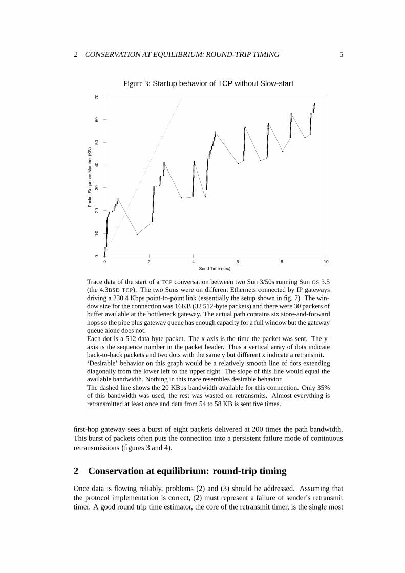
Trace data of the start of aTCP conversation between two Sun 3/50s running SunOS 3.5(the 4.3BSD TCP). The two Suns were on different Ethernets connected by IP gatewaysdriving a 230.4 Kbps point-to-point link (essentially the setup shown in fig. 7). The win-dow size for the connection was 16KB (32 512-byte packets) and there were 30 packets ofbuffer available at the bottleneck gateway. The actual path contains six store-and-forwardhops so the pipe plus gateway queue has enough capacity for a full window but the gatewayqueue alone does not.Each dot is a 512 data-byte packet. The x-axis is the time the packet was sent. The y-axis is the sequence number in the packet header. Thus a vertical array of dots indicateback-to-back packets and two dots with the same y but different x indicate a retransmit.‘Desirable’ behavior on this graph would be a relatively smooth line of dots extendingdiagonally from the lower left to the upper right. The slope of this line would equal theavailable bandwidth. Nothing in this trace resembles desirable behavior.The dashed line shows the 20 KBps bandwidth available for this connection. Only 35%of this bandwidth was used; the rest was wasted on retransmits. Almost everything isretransmitted at least once and data from 54 to 58 KB is sent five times.

first-hop gateway sees a burst of eight packets delivered at 200 times the path bandwidth.This burst of packets often puts the connection into a persistent failure mode of continuousretransmissions (figures 3 and 4).

2 Conservation at equilibrium: round-trip timing

Once data is flowing reliably, problems (2) and (3) should be addressed. Assuming thatthe protocol implementation is correct, (2) must represent a failure of sender’s retransmittimer. A good round trip time estimator, the core of the retransmit timer, is the single most


Figure 4:Startup behavior of TCP with Slow-start

• •• ••• ••••••••••••• •••••

••••••••••••••••••••••• ••• •••••

•••••••••••••••••••• •••••

•••••••••••••••

•••••••••••• •••• •••••

•••••••••••••••

••••••• • •••••

••••• •••••••••••••••

••••••••••

••••••• •••••

•••••••••••••••

••••••••••

•• ••••••••••

•••••••••••

••••••••••• •••••

••••••••••

••••••••••

•••••• ••• •••••

•• ••••••••••

••••••••••

••

Send Time (sec)

Pac

ket S

eque

nce

Num

ber

(KB

)

0 2 4 6 8 10

020

4060

8010

012

014

016

0

Same conditions as the previous figure (same time of day, same Suns, same network path,same buffer and window sizes), except the machines were running the 4.3+TCPwith slow-start. No bandwidth is wasted on retransmits but two seconds is spent on the slow-startso the effective bandwidth of this part of the trace is 16 KBps — two times better thanfigure 3. (This is slightly misleading: Unlike the previous figure, the slope of the trace is20 KBps and the effect of the 2 second offset decreases as the trace lengthens. E.g., if thistrace had run a minute, the effective bandwidth would have been 19 KBps. The effectivebandwidth without slow-start stays at 7 KBps no matter how long the trace.)

important feature of any protocol implementation that expects to survive heavy load. Andit is frequently botched ([26] and [13] describe typical problems).

One mistake is not estimating the variation,σR, of the round trip time,R. From queuingtheory we know thatR and the variation inR increase quickly with load. If the load isρ(the ratio of average arrival rate to average departure rate),R andσR scale like(1−ρ)−1.To make this concrete, if the network is running at 75% of capacity, as the Arpanet was inlast April’s collapse, one should expect round-trip-time to vary by a factor of sixteen (−2σto +2σ).

TheTCPprotocol specification[2] suggests estimating mean round trip time via the low-pass filter

R← αR+(1−α)M

whereR is the averageRTT estimate,M is a round trip time measurement from the mostrecently acked data packet, andα is a filter gain constant with a suggested value of 0.9.Once theRestimate is updated, the retransmit timeout interval,rto, for the next packet sentis set toβR.


Figure 5:Performance of an RFC793 retransmit timer

•

• • • •

••

• •

• •

• •

••• •

• •

••

• • • • ••

•••

• • • • •

• ••

••

• • • • • •

••

• • •

• ••

•

• ••

•

•••

•

• ••

•

• • •

•• •

•••

• •

•• •

•

• •

••

••

• • •

• • •

•

•

••

•

• •

Packet

RT

T (

sec.

)

0 10 20 30 40 50 60 70 80 90 100 110

02

46

810

12

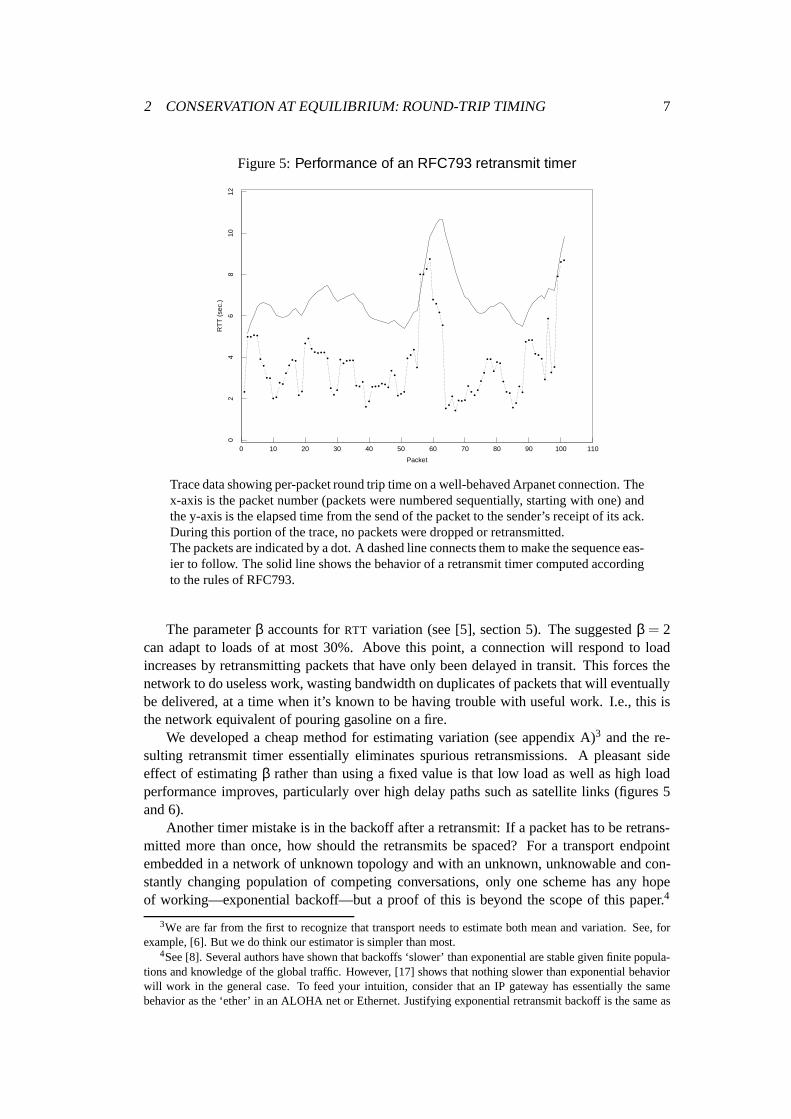
Trace data showing per-packet round trip time on a well-behaved Arpanet connection. Thex-axis is the packet number (packets were numbered sequentially, starting with one) andthe y-axis is the elapsed time from the send of the packet to the sender’s receipt of its ack.During this portion of the trace, no packets were dropped or retransmitted.The packets are indicated by a dot. A dashed line connects them to make the sequence eas-ier to follow. The solid line shows the behavior of a retransmit timer computed accordingto the rules of RFC793.

The parameterβ accounts forRTT variation (see [5], section 5). The suggestedβ = 2can adapt to loads of at most 30%. Above this point, a connection will respond to loadincreases by retransmitting packets that have only been delayed in transit. This forces thenetwork to do useless work, wasting bandwidth on duplicates of packets that will eventuallybe delivered, at a time when it’s known to be having trouble with useful work. I.e., this isthe network equivalent of pouring gasoline on a fire.

We developed a cheap method for estimating variation (see appendix A)3 and the re-sulting retransmit timer essentially eliminates spurious retransmissions. A pleasant sideeffect of estimatingβ rather than using a fixed value is that low load as well as high loadperformance improves, particularly over high delay paths such as satellite links (figures 5and 6).

Another timer mistake is in the backoff after a retransmit: If a packet has to be retrans-mitted more than once, how should the retransmits be spaced? For a transport endpointembedded in a network of unknown topology and with an unknown, unknowable and con-stantly changing population of competing conversations, only one scheme has any hopeof working—exponential backoff—but a proof of this is beyond the scope of this paper.4

3We are far from the first to recognize that transport needs to estimate both mean and variation. See, forexample, [6]. But we do think our estimator is simpler than most.

4See [8]. Several authors have shown that backoffs ‘slower’ than exponential are stable given finite popula-tions and knowledge of the global traffic. However, [17] shows that nothing slower than exponential behaviorwill work in the general case. To feed your intuition, consider that an IP gateway has essentially the samebehavior as the ‘ether’ in an ALOHA net or Ethernet. Justifying exponential retransmit backoff is the same as

3 ADAPTING TO THE PATH: CONGESTION AVOIDANCE 8

Figure 6:Performance of a Mean+Variance retransmit timer

•

• • • •

••

• •

• •

• •

••• •

• •

••

• • • • ••

•••

• • • • •

• ••

••

• • • • • •

••

• • •

• ••

•

• ••

•

•••

•

• ••

•

• • •

•• •

•••

• •

•• •

•

• •

••

••

• • •

• • •

•

•

••

•

• •

Packet

RT

T (

sec.

)

0 10 20 30 40 50 60 70 80 90 100 110

02

46

810

12

Same data as above but the solid line shows a retransmit timer computed according to thealgorithm in appendix A.

To finesse a proof, note that a network is, to a very good approximation, a linear system.That is, it is composed of elements that behave like linear operators — integrators, delays,gain stages, etc. Linear system theory says that if a system is stable, the stability is expo-nential. This suggests that an unstable system (a network subject to random load shocksand prone to congestive collapse5) can be stabilized by adding some exponential damping(exponential timer backoff) to its primary excitation (senders, traffic sources).

3 Adapting to the path: congestion avoidance

If the timers are in good shape, it is possible to state with some confidence that a timeout in-dicates a lost packet and not a broken timer. At this point, something can be done about (3).Packets get lost for two reasons: they are damaged in transit, or the network is congestedand somewhere on the path there was insufficient buffer capacity. On most network paths,loss due to damage is rare (�1%) so it is probable that a packet loss is due to congestion inthe network.6

showing that no collision backoff slower than an exponential will guarantee stability on an Ethernet. Unfortu-nately, with an infinite user population even exponential backoff won’t guarantee stability (although it ‘almost’does—see [1]). Fortunately, we don’t (yet) have to deal with an infinite user population.

5The phrasecongestion collapse(describing a positive feedback instability due to poor retransmit timers) isagain the coinage of John Nagle, this time from [23].

6Because a packet loss empties the window, the throughput of any window flow control protocol is quitesensitive to damage loss. For an RFC793 standard TCP running with windoww (wherew is at most thebandwidth-delay product), a loss probability ofp degrades throughput by a factor of(1+2pw)−1. E.g., a 1%damage loss rate on an Arpanet path (8 packet window) degradesTCP throughput by 14%.

The congestion control scheme we propose is insensitive to damage loss until the loss rate is on the order ofthe window equilibration length (the number of packets it takes the window to regain its original size after aloss). If the pre-loss size isw, equilibration takes roughlyw2/3 packets so, for the Arpanet, the loss sensitivity


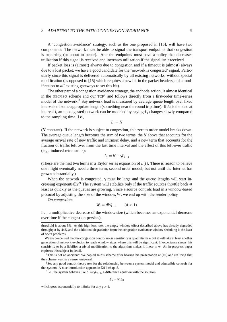
A ‘congestion avoidance’ strategy, such as the one proposed in [15], will have twocomponents: The network must be able to signal the transport endpoints that congestionis occurring (or about to occur). And the endpoints must have a policy that decreasesutilization if this signal is received and increases utilization if the signal isn’t received.

If packet loss is (almost) always due to congestion and if a timeout is (almost) alwaysdue to a lost packet, we have a good candidate for the ‘network is congested’ signal. Partic-ularly since this signal is delivered automatically by all existing networks, without specialmodification (as opposed to [15] which requires a new bit in the packet headers and a mod-ification toall existing gateways to set this bit).

The other part of a congestion avoidance strategy, the endnode action, is almost identicalin the DEC/ISO scheme and ourTCP7 and follows directly from a first-order time-seriesmodel of the network:8 Say network load is measured by average queue length over fixedintervals of some appropriate length (something near the round trip time). IfLi is the load atinterval i, an uncongested network can be modeled by sayingLi changes slowly comparedto the sampling time. I.e.,

Li = N

(N constant). If the network is subject to congestion, this zeroth order model breaks down.The average queue length becomes the sum of two terms, theN above that accounts for theaverage arrival rate of new traffic and intrinsic delay, and a new term that accounts for thefraction of traffic left over from the last time interval and the effect of this left-over traffic(e.g., induced retransmits):

Li = N+ γLi−1

(These are the first two terms in a Taylor series expansion ofL(t). There is reason to believeone might eventually need a three term, second order model, but not until the Internet hasgrown substantially.)

When the network is congested,γ must be large and the queue lengths will start in-creasing exponentially.9 The system will stabilize only if the traffic sources throttle back atleast as quickly as the queues are growing. Since a source controls load in a window-basedprotocol by adjusting the size of the window,W, we end up with the sender policy

On congestion:Wi = dWi−1 (d < 1)

I.e., a multiplicative decrease of the window size (which becomes an exponential decreaseover time if the congestion persists).

threshold is about 5%. At this high loss rate, the empty window effect described above has already degradedthroughput by 44% and the additional degradation from the congestion avoidance window shrinking is the leastof one’s problems.

We are concerned that the congestion control noise sensitivity is quadratic inw but it will take at least anothergeneration of network evolution to reach window sizes where this will be significant. If experience shows thissensitivity to be a liability, a trivial modification to the algorithm makes it linear inw. An in-progress paperexplores this subject in detail.

7This is not an accident: We copied Jain’s scheme after hearing his presentation at [10] and realizing thatthe scheme was, in a sense, universal.

8See any good control theory text for the relationship between a system model and admissible controls forthat system. A nice introduction appears in [21], chap. 8.

9I.e., the system behaves likeLi ≈ γLi−1, a difference equation with the solution

Ln = γnL0

which goes exponentially to infinity for anyγ > 1.


If there’s no congestion,γ must be near zero and the load approximately constant. Thenetwork announces, via a dropped packet, when demand is excessive but says nothing if aconnection is using less than its fair share (since the network is stateless, it cannot knowthis). Thus a connection has to increase its bandwidth utilization to find out the currentlimit. E.g., you could have been sharing the path with someone else and converged to awindow that gives you each half the available bandwidth. If she shuts down, 50% of thebandwidth will be wasted unless your window size is increased. What should the increasepolicy be?

The first thought is to use a symmetric, multiplicative increase, possibly with a longertime constant,Wi = bWi−1, 1 < b≤ 1/d. This is a mistake. The result will oscillate wildlyand, on the average, deliver poor throughput. The analytic reason for this has to do withthat fact that it is easy to drive the net into saturation but hard for the net to recover (what[18], chap. 2.1, calls therush-hour effect).10 Thus overestimating the available bandwidthis costly. But an exponential, almost regardless of its time constant, increases so quicklythat overestimates are inevitable.

Without justification, we’ll state that the best increase policy is to make small, constantchanges to the window size:11

On no congestion:Wi = Wi−1 +u (u�Wmax)

whereWmax is thepipesize(the delay-bandwidth product of the path minus protocol over-head — i.e., the largest sensible window for the unloaded path). This is the additive increase/ multiplicative decrease policy suggested in [15] and the policy we’ve implemented inTCP.The only difference between the two implementations is the choice of constants ford andu.We used 0.5 and 1 for reasons partially explained in appendix D. A more complete analysisis in yet another in-progress paper.

The preceding has probably made the congestion control algorithm sound hairy but it’snot. Like slow-start, it’s three lines of code:

• On any timeout, setcwnd to half the current window size (this is the multiplicativedecrease).

• On each ack for new data, increasecwndby 1/cwnd(this is the additive increase).12

10In fig. 1, note that the ‘pipesize’ is 16 packets, 8 in each path, but the sender is using a window of 22packets. The six excess packets will form a queue at the entry to the bottleneck andthat queue cannot shrink,even though the sender carefully clocks out packets at the bottleneck link rate. This stable queue is another,unfortunate, aspect of conservation: The queue would shrink only if the gateway could move packets into theskinny pipe faster than the sender dumped packets into the fat pipe. But the system tunes itself so each time thegateway pulls a packet off the front of its queue, the sender lays a new packet on the end.

A gateway needs excess output capacity (i.e.,ρ < 1) to dissipate a queue and the clearing time will scalelike (1−ρ)−2 ([18], chap. 2 is an excellent discussion of this). Since at equilibrium our transport connection‘wants’ to run the bottleneck link at 100% (ρ = 1), we have to be sure that during the non-equilibrium windowadjustment, our control policy allows the gateway enough free bandwidth to dissipate queues that inevitablyform due to path testing and traffic fluctuations. By an argument similar to the one used to show exponentialtimer backoff is necessary, it’s possible to show that an exponential (multiplicative) window increase policywill be ‘faster’ than the dissipation time for some traffic mix and, thus, leads to an unbounded growth of thebottleneck queue.

11See [4] for a complete analysis of these increase and decrease policies. Also see [8] and [9] for a control-theoretic analysis of a similar class of control policies.

12This increment rule may be less than obvious. We want to increase the window by at most one packet overa time interval of lengthR (the round trip time). To make the algorithm ‘self-clocked’, it’s better to incrementby a small amount on each ack rather than by a large amount at the end of the interval. (Assuming, of course,

4 THE GATEWAY SIDE OF CONGESTION CONTROL 11

• When sending, send the minimum of the receiver’s advertised window andcwnd.

Note that this algorithm isonly congestion avoidance, it doesn’t include the previouslydescribed slow-start. Since the packet loss that signals congestion will result in a re-start, itwill almost certainly be necessary to slow-start in addition to the above. But, because bothcongestion avoidance and slow-start are triggered by a timeout and both manipulate thecongestion window, they are frequently confused. They are actually independent algorithmswith completely different objectives. To emphasize the difference, the two algorithms havebeen presented separately even though in practise they should be implemented together.Appendix B describes a combined slow-start/congestion avoidance algorithm.13

Figures 7 through 12 show the behavior ofTCPconnections with and without congestionavoidance. Although the test conditions (e.g., 16 KB windows) were deliberately chosento stimulate congestion, the test scenario isn’t far from common practice: The ArpanetIMP

end-to-end protocol allows at most eight packets in transit between any pair of gateways.The default 4.3BSD window size is eight packets (4 KB). Thus simultaneous conversationsbetween, say, any two hosts at Berkeley and any two hosts atMIT would exceed the networkcapacity of theUCB–MIT IMP path and would lead14 to the type of behavior shown.

4 Future work: the gateway side of congestion control

While algorithms at the transport endpoints can insure the network capacity isn’t exceeded,they cannot insure fair sharing of that capacity. Only in gateways, at the convergence offlows, is there enough information to control sharing and fair allocation. Thus, we view thegateway ‘congestion detection’ algorithm as the next big step.

the sender has effectivesilly windowavoidance (see [5], section 3) and doesn’t attempt to send packet fragmentsbecause of the fractionally sized window.) A window of sizecwndpackets will generate at mostcwndacks inoneR. Thus an increment of 1/cwndper ack will increase the window by at most one packet in oneR. In TCP,windows and packet sizes are in bytes so the increment translates tomaxseg*maxseg/cwndwheremaxsegis themaximum segment size andcwndis expressed in bytes, not packets.

13We have also developed a rate-based variant of the congestion avoidance algorithm to apply to connection-less traffic (e.g., domain server queries,RPCrequests). Remembering that the goal of the increase and decreasepolicies is bandwidth adjustment, and that ‘time’ (the controlled parameter in a rate-based scheme) appears inthe denominator of bandwidth, the algorithm follows immediately: The multiplicative decrease remains a mul-tiplicative decrease (e.g., double the interval between packets). But subtracting a constant amount from intervaldoesnot result in an additive increase in bandwidth. This approach has been tried, e.g., [19] and [24], andappears to oscillate badly. To see why, note that for an inter-packet intervalI and decrementc, the bandwidthchange of a decrease-interval-by-constant policy is

1I→ 1

I −c

a non-linear, and destablizing, increase.An update policy that does result in a linear increase of bandwidth over time is

Ii =αIi−1

α+ Ii−1

whereIi is the interval between sends when theith packet is sent andα is the desired rate of increase in packetsper packet/sec.

We have simulated the above algorithm and it appears to perform well. To test the predictions of that simula-tion against reality, we have a cooperative project with Sun Microsystems to prototypeRPCdynamic congestioncontrol algorithms usingNFS as a test-bed (sinceNFS is known to have congestion problems yet it would bedesirable to have it work over the same range of networks asTCP).

14did lead.


Figure 7:Multiple conversation test setup

Polo(sun 3/50)

Hot(sun 3/50)

Surf(sun 3/50)

Renoir(vax 750)

VanGogh(vax 8600)

Monet(vax 750)

Okeeffe(CCI)

Vs(sun 3/50)

csam cartan230.4 KbsMicrowave

10 Mbs Ethernets

Test setup to examine the interaction of multiple, simultaneousTCP conversations sharinga bottleneck link. 1 MByte transfers (2048 512-data-byte packets) were initiated 3 secondsapart from four machines at LBL to four machines at UCB, one conversation per machinepair (the dotted lines above show the pairing). All traffic went via a 230.4 Kbps linkconnecting IP routercsamat LBL to IP routercartan at UCB. The microwave link queuecan hold up to 50 packets. Each connection was given a window of 16 KB (32 512-bytepackets). Thus any two connections could overflow the available buffering and the fourconnections exceeded the queue capacity by 160%.

The goal of this algorithm to send a signal to the endnodes as early as possible, butnot so early that the gateway becomes starved for traffic. Since we plan to continue usingpacket drops as a congestion signal, gateway ‘self protection’ from a mis-behaving hostshould fall-out for free: That host will simply have most of its packets dropped as the gate-way trys to tell it that it’s using more than its fair share. Thus, like the endnode algorithm,the gateway algorithm should reduce congestion even if no endnode is modified to do con-gestion avoidance. And nodes that do implement congestion avoidance will get their fairshare of bandwidth and a minimum number of packet drops.

Since congestion grows exponentially, detecting it early is important. If detected early,small adjustments to the senders’ windows will cure it. Otherwise massive adjustmentsare necessary to give the net enough spare capacity to pump out the backlog. But, giventhe bursty nature of traffic, reliable detection is a non-trivial problem. Jain[15] proposesa scheme based on averaging between queue regeneration points. This should yield goodburst filtering but we think it might have convergence problems under high load or sig-nificant second-order dynamics in the traffic.15 We plan to use some of our earlier workon ARMAX models for round-trip-time/queue length prediction as the basis of detection.

15These problems stem from the fact that the average time between regeneration points scales like(1−ρ)−1

and the variance like(1−ρ)−3 (see Feller[7], chap. VI.9). Thus the congestion detector becomes sluggish ascongestion increases and its signal-to-noise ratio decreases dramatically.


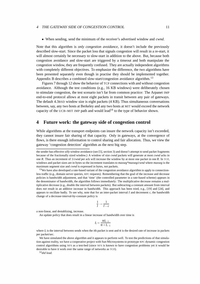
Figure 8:Multiple, simultaneous TCPs with no congestion avoidance

Time (sec)

Seq

uenc

e N

umbe

r (K

B)

0 50 100 150 200

020

040

060

080

010

0012

00

Trace data from four simultaneousTCP conversations without congestion avoidance overthe paths shown in figure 7. 4,000 of 11,000 packets sent were retransmissions (i.e., halfthe data packets were retransmitted). Since the link data bandwidth is 25 KBps, each of thefour conversations should have received 6 KBps. Instead, one conversation got 8 KBps,two got 5 KBps, one got 0.5 KBps and 6 KBps has vanished.

Preliminary results suggest that this approach works well at high load, is immune to second-order effects in the traffic and is computationally cheap enough to not slow down kilopacket-per-second gateways.

Acknowledgements

We are grateful to the members of the Internet Activity Board’s End-to-End and Internet-Engineering task forces for this past year’s interest, encouragement, cogent questions andnetwork insights. Bob Braden of ISI and Craig Partridge of BBN were particularly helpfulin the preparation of this paper: their careful reading of early drafts improved it immensely.

The first author is also deeply in debt to Jeff Mogul of DEC Western Research Lab.Without Jeff’s interest and patient prodding, this paper would never have existed.


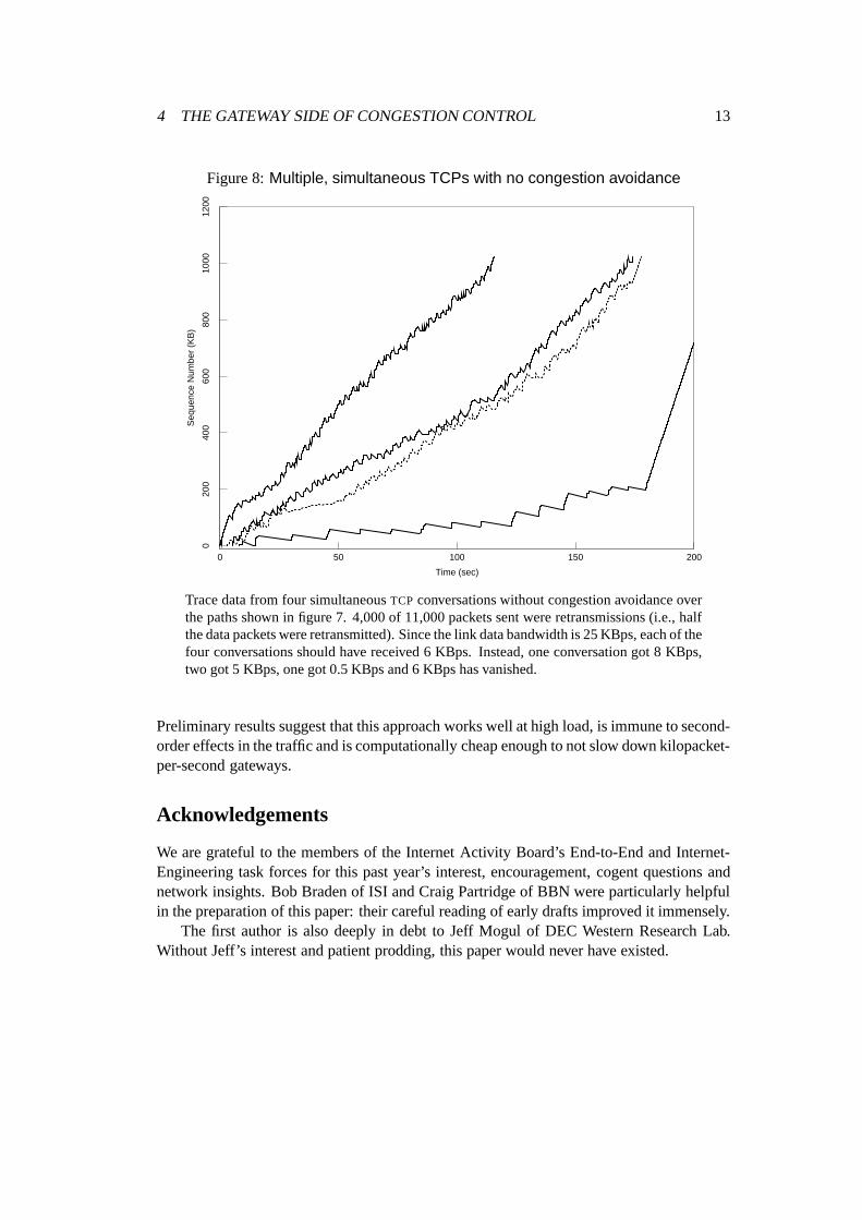
Figure 9:Multiple, simultaneous TCPs with congestion avoidance

Time (sec)

Seq

uenc

e N

umbe

r (K

B)

0 50 100 150 200

020

040

060

080

010

0012

00

Trace data from four simultaneousTCPconversations using congestion avoidance over thepaths shown in figure 7. 89 of 8281 packets sent were retransmissions (i.e., 1% of the datapackets had to be retransmitted). Two of the conversations got 8 KBps and two got 4.5KBps (i.e., all the link bandwidth is accounted for — see fig. 11). The difference betweenthe high and low bandwidth senders was due to the receivers. The 4.5 KBps senders weretalking to 4.3BSD receivers which would delay an ack until 35% of the window was filledor 200 ms had passed (i.e., an ack was delayed for 5–7 packets on the average). This meantthe sender would deliver bursts of 5–7 packets on each ack.The 8 KBps senders were talking to 4.3+BSD receivers which would delay an ack for atmost one packet (because of an ack’s ‘clock’ rˆole, the authors believe that the minimumack frequency should be every other packet). I.e., the sender would deliver bursts ofat most two packets. The probability of loss increases rapidly with burst size so senderstalking to old-style receivers saw three times the loss rate (1.8% vs. 0.5%). The higher lossrate meant more time spent in retransmit wait and, because of the congestion avoidance,smaller average window sizes.


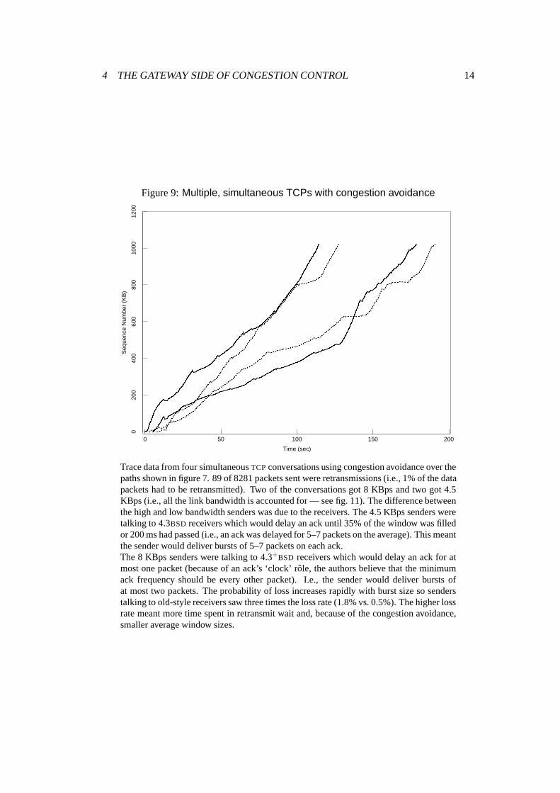
Figure 10:Total bandwidth used by old and new TCPs

Time (sec)

Rel

ativ

e B

andw

idth

0 20 40 60 80 100 120

0.8

1.0

1.2

1.4

1.6

The thin line shows the total bandwidth used by the four senders without congestionavoidance (fig. 8), averaged over 5 second intervals and normalized to the 25 KBps linkbandwidth. Note that the senders send, on the average, 25% more than will fit in the wire.The thick line is the same data for the senders with congestion avoidance (fig. 9). Thefirst 5 second interval is low (because of the slow-start), then there is about 20 secondsof damped oscillation as the congestion control ‘regulator’ for eachTCP finds the correctwindow size. The remaining time the senders run at the wire bandwidth. (The activityaround 110 seconds is a bandwidth ‘re-negotiation’ due to connection one shutting down.The activity around 80 seconds is a reflection of the ‘flat spot’ in fig. 9 where most ofconversation two’s bandwidth is suddenly shifted to conversations three and four — com-peting conversations frequently exhibit this type of ‘punctuated equilibrium’ behavior andwe hope to investigate its dynamics in a future paper.)


Figure 11:Effective bandwidth of old and new TCPs

Time (sec)

Rel

ativ

e B

andw

idth

0 20 40 60 80 100 120

0.5

0.6

0.7

0.8

0.9

1.0

1.1

1.2

Figure 10 showed the oldTCPs were using 25% more than the bottleneck link bandwidth.Thus, once the bottleneck queue filled, 25% of the the senders’ packets were being dis-carded. If the discards, and only the discards, were retransmitted, the senders would havereceived the full 25 KBps link bandwidth (i.e., their behavior would have been anti-socialbut not self-destructive). But fig. 8 noted that around 25% of the link bandwidth was un-accounted for. Here we average the total amount of data acked per five second interval.(This gives theeffectiveor deliveredbandwidth of the link.) The thin line is once again theold TCPs. Note that only 75% of the link bandwidth is being used for data (the remaindermust have been used by retransmissions of packets that didn’t need to be retransmitted).The thick line shows delivered bandwidth for the newTCPs. There is the same slow-startand turn-on transient followed by a long period of operation right at the link bandwidth.


Figure 12:Window adjustment detail

•

••

•

•

•

• •• •

•

•

•

•• •

• •

•

•

••

• ••

•

Time (sec)

Rel

ativ

e B

andw

idth

0 20 40 60 800.4

0.6

0.8

1.0

1.2

1.4

Because of the five second averaging time (needed to smooth out the spikes in the oldTCP

data), the congestion avoidance window policy is difficult to make out in figures 10 and11. Here we show effective throughput (data acked) forTCPs with congestion control,averaged over a three second interval.When a packet is dropped, the sender sends until it fills the window, then stops until theretransmission timeout. Since the receiver cannot ack data beyond the dropped packet, onthis plot we’d expect to see a negative-going spike whose amplitude equals the sender’swindow size (minus one packet). If the retransmit happens in the next interval (the in-tervals were chosen to match the retransmit timeout), we’d expect to see a positive-goingspike of the same amplitude when receiver acks the out-of-order data it cached. Thus theheight of these spikes is a direct measure of the sender’s window size.The data clearly shows three of these events (at 15, 33 and 57 seconds) and the windowsize appears to be decreasing exponentially. The dotted line is a least squares fit to thesix window size measurements obtained from these events. The fit time constant was 28seconds. (The long time constant is due to lack of a congestion avoidance algorithm inthe gateway. With a ‘drop’ algorithm running in the gateway, the time constant should bearound 4 seconds)

A A FAST ALGORITHM FOR RTT MEAN AND VARIATION 18

A A fast algorithm for rtt mean and variation

A.1 Theory

The RFC793 algorithm for estimating the mean round trip time is one of the simplestexamples of a class of estimators calledrecursive prediction erroror stochastic gradientalgorithms. In the past 20 years these algorithms have revolutionized estimation and con-trol theory [20] and it’s probably worth looking at the RFC793 estimator in some detail.

Given a new measurementm of the RTT (round trip time),TCP updates an estimate ofthe averageRTT a by

a← (1−g)a+gm

whereg is a ‘gain’ (0< g < 1) that should be related to the signal-to-noise ratio (or, equiv-alently, variance) ofm. This makes a more sense, and computes faster, if we rearrange andcollect terms multiplied byg to get

a← a+g(m−a)

Think of a as a prediction of the next measurement.m− a is the error in that predictionand the expression above says we make a new prediction based on the old prediction plussome fraction of the prediction error. The prediction error is the sum of two components:(1) error due to ‘noise’ in the measurement (random, unpredictable effects like fluctuationsin competing traffic) and (2) error due to a bad choice ofa. Calling the random errorEr andthe estimation errorEe,

a← a+gEr +gEe

The gEe term givesa a kick in the right direction while thegEr term gives it a kick in arandom direction. Over a number of samples, the random kicks cancel each other out sothis algorithm tends to converge to the correct average. Butg represents a compromise:We want a largeg to get mileage out ofEe but a smallg to minimize the damage fromEr .Since theEe terms movea toward the real average no matter what value we use forg, it’salmost always better to use a gain that’s too small rather than one that’s too large. Typicalgain choices are 0.1–0.2 (though it’s a good idea to take long look at your raw data beforepicking a gain).

It’s probably obvious thata will oscillate randomly around the true average and thestandard deviation ofa will be gsdev(m). Also thata converges to the true average expo-nentially with time constant 1/g. So a smallerg gives a stablera at the expense of taking amuch longer time to get to the true average.

If we want some measure of the variation inm, say to compute a good value for theTCP retransmit timer, there are several alternatives. Variance,σ2, is the conventional choicebecause it has some nice mathematical properties. But computing variance requires squar-ing (m−a) so an estimator for it will contain a multiply with a danger of integer overflow.Also, most applications will want variation in the same units asa andm, so we’ll be forcedto take the square root of the variance to use it (i.e., at least a divide, multiply and two adds).

A variation measure that’s easy to compute is the mean prediction error or mean devia-tion, the average of|m−a|. Also, since

mdev2 =(∑ |m−a|)2 ≥ ∑ |m−a|2 = σ2

A A FAST ALGORITHM FOR RTT MEAN AND VARIATION 19

mean deviation is a more conservative (i.e., larger) estimate of variation than standarddeviation.16

There’s often a simple relation between mdev and sdev. E.g., if the prediction errors arenormally distributed,mdev=

√π/2sdev. For most common distributions the factor to go

from sdevto mdevis near one (√

π/2≈ 1.25). I.e.,mdevis a good approximation ofsdevand is much easier to compute.

A.2 Practice

Fast estimators for averagea and mean deviationv given measurementm follow directlyfrom the above. Both estimators compute means so there are two instances of the RFC793algorithm:

Err ≡m−a

a← a+gErr

v← v+g(|Err|−v)

To be computed quickly, the above should be done in integer arithmetic. But the ex-pressions contain fractions (g < 1) so some scaling is needed to keep everything integer. Areciprocal power of 2 (i.e.,g = 1/2n for somen) is a particularly good choice forg sincethe scaling can be implemented with shifts. Multiplying through by 1/g gives

2na← 2na+Err

2nv← 2nv+(|Err|−v)

To minimize round-off error, the scaled versions ofa and v, sa and sv, should bekept rather than the unscaled versions. Pickingg = .125= 1

8 (close to the .1 suggestedin RFC793) and expressing the above in C:

/∗ update Average estimator∗/m −= (sa >> 3);sa += m;/∗ update Deviation estimator∗/if (m < 0)

m = −m;m −= (sv >> 3);sv += m;

It’s not necessary to use the same gain fora andv. To force the timer to go up quicklyin response to changes in theRTT, it’s a good idea to givev a larger gain. In particular,because of window–delay mismatch there are oftenRTT artifacts at integer multiples of thewindow size.17 To filter these, one would like 1/g in thea estimator to be at least as largeas the window size (in packets) and 1/g in thev estimator to be less than the window size.18

16Purists may note that we elided a factor of 1/n, the number of samples, from the previous inequality. Itmakes no difference to the result.

17E.g., see packets 10–50 of figure 5. Note that these window effects are due to characteristics of theArpa/Milnet subnet. In general, window effects on the timer are at most a second-order consideration anddepend a great deal on the underlying network. E.g., if one were using the Wideband with a 256 packet win-dow, 1/256 would not be a good gain fora (1/16 might be).

18Although it may not be obvious, the absolute value in the calculation ofv introduces an asymmetry in thetimer: Becausev has the same sign as an increase and the opposite sign of a decrease, more gain inv makes the

B SLOW-START + CONGESTION AVOIDANCE ALGORITHM 20

Using a gain of .25 on the deviation and computing the retransmit timer,rto, asa+4v,the final timer code looks like:

m −= (sa >> 3);sa += m;if (m < 0)

m = −m;m −= (sv >> 2);sv += m;rto = (sa >> 3) + sv;

In general this computation will correctly roundrto: Because of thesa truncation whencomputingm−a, sawill converge to the true mean rounded up to the next tick. Likewisewith sv. Thus, on the average, there is half a tick of bias in each. Therto computationshould be rounded by half a tick and one tick needs to be added to account for sends beingphased randomly with respect to the clock. So, the 1.75 tick bias contribution from 4vapproximately equals the desired half tick rounding plus one tick phase correction.

B The combined slow-start with congestion avoidancealgorithm

The sender keeps two state variables for congestion control: a slow-start/congestion win-dow, cwnd, and a threshold size,ssthresh, to switch between the two algorithms. Thesender’s output routine always sends the minimum ofcwndand the window advertised bythe receiver. On a timeout, half the current window size is recorded inssthresh(this is themultiplicative decrease part of the congestion avoidance algorithm), thencwnd is set to 1packet (this initiates slow-start). When new data is acked, the sender does

if (cwnd < ssthresh)/∗ if we’re still doing slow−start∗ open window exponentially∗/

cwnd += 1;else

/∗ otherwise do Congestion∗ Avoidance increment−by−1 ∗/

cwnd += 1/cwnd;

Thus slow-start opens the window quickly to what congestion avoidance thinks is a safeoperating point (half the window that got us into trouble), then congestion avoidance takesover and slowly increases the window size to probe for more bandwidth becoming availableon the path.

Note that theelseclause of the above code will malfunction ifcwnd is an integer inunscaled, one-packet units. I.e., if the maximum window for the path isw packets,cwnd

timer go up quickly and come down slowly, ‘automatically’ giving the behavior suggested in [22]. E.g., see theregion between packets 50 and 80 in figure 6.

C INTERACTION OF WINDOW ADJUSTMENT WITH ROUND-TRIP TIMING 21

must cover the range 0..w with resolution of at least 1/w.19 Since sending packets smallerthan the maximum transmission unit for the path lowers efficiency, the implementor musttake care that the fractionally sizedcwnddoesnot result in small packets being sent. InreasonableTCP implementations, existing silly-window avoidance code should prevent runtpackets but this point should be carefully checked.

C Interaction of window adjustment with round-trip timing

SomeTCP connections, particularly those over a very low speed link such as a dial-up SLIPline[25], may experience an unfortunate interaction between congestion window adjustmentand retransmit timing: Network paths tend to divide into two classes:delay-dominated,where the store-and-forward and/or transit delays determine theRTT, andbandwidth-dominated,where (bottleneck) link bandwidth and average packet size determine theRTT.20 On abandwidth-dominated path of bandwidthb, a congestion-avoidance window increment of∆w will increase theRTT of post-increment packets by

∆R≈ ∆wb

If the pathRTT variationV is small,∆R may exceed the 4V cushion inrto, a retransmittimeout will occur and, after a few cycles of this,ssthresh(and, thus,cwnd) end up clampedat small values.

Therto calculation in appendix A was designed to prevent this type of spurious retrans-mission timeout during slow-start. In particular, theRTT variationV is multiplied by fourin therto calculation because of the following: A spurious retransmit occurs if the retrans-mit timeout computed at the end of slow-start roundi, rtoi , is ever less than or equal tothe actualRTT of the next round. In the worst case of all the delay being due the window,R doubles each round (since the window size doubles). ThusRi+1 = 2Ri (whereRi is themeasuredRTT at slow-start roundi). But

Vi = Ri−Ri−1

= Ri/2

and

rtoi = Ri +4Vi

= 3Ri

> 2Ri

> Ri+1

so spurious retransmit timeouts cannot occur.21

19For TCP this happens automatically since windows are expressed in bytes, not packets. For protocolssuch as ISO TP4, the implementor should scalecwndso that the calculations above can be done with integerarithmetic and the scale factor should be large enough to avoid the fixed point (zero) ofb1/cwndc in thecongestion avoidance increment.

20E.g., TCP over a 2400 baud packet radio link is bandwidth-dominated since the transmission time for a(typical) 576 byte IP packet is 2.4 seconds, longer than any possible terrestrial transit delay.

21The original SIGCOMM ’88 version of this paper suggested calculatingrto asR+ 2V rather thanR+4V. Since that time we have had much more experience with low speed SLIP links and observed spuriousretransmissions during connection startup. An investigation of why these occured led to the analysis above andthe change to therto calculation in app. A.

D WINDOW ADJUSTMENT POLICY 22

Spurious retransmission due to a window increase can occur during the congestionavoidance window increment since the window can only be changed in one packet incre-ments so, for a packet sizes, there may be as many ass−1 packets between increments,long enough for anyV increase due to the last window increment to decay away to nothing.But this problem is unlikely on a bandwidth-dominated path since the increments wouldhave to be more than twelve packets apart (the decay time of theV filter times its gain in therto calculation) which implies that a ridiculously large window is being used for the path.22

Thus one should regard these timeouts as appropriate punishment for gross mis-tuning andtheir effect will simply be to reduce the window to something more appropriate for the path.

Although slow-start and congestion avoidance are designed to not trigger this kind ofspurious retransmission, an interaction with higher level protocols frequently does: Appli-cation protocols likeSMTP andNNTP have a ‘negotiation’ phase where a few packets areexchanged stop-and-wait, followed by data transfer phase where all of a mail message ornews article is sent. Unfortunately, the ‘negotiation’ exchanges open the congestion win-dow so the start of the data transfer phase will dump several packets into the network withno slow-start and, on a bandwidth-dominated path, faster thanrto can track theRTT in-crease caused by these packets. The root cause of this problem is the same one describedin sec. 1: dumping too many packets into an empty pipe (the pipe is empty since the ne-gotiation exchange was conducted stop-and-wait) with no ack ‘clock’. The fix proposed insec. 1, slow-start, will also prevent this problem if theTCP implementation can detect thephase change. And detection is simple: The pipe is empty because we haven’t sent anythingfor at least a round-trip-time (another way to viewRTT is as the time it takes the pipe toempty after the most recent send). So, if nothing has been sent for at least oneRTT, thenext send should setcwnd to one packet to force a slow-start. I.e., if the connection statevariablelastsndholds the time the last packet was sent, the following code should appearearly in theTCP output routine:

int idle = (snd max == snduna);if (idle && now − lastsnd> rto)

cwnd = 1;

The booleanidle is true if there is no data in transit (all data sent has been acked) so theifsays “if there’s nothing in transit and we haven’t sent anything for ‘a long time’, slow-start.”Our experience has been that either the currentRTT estimate or therto estimate can be usedfor ‘a long time’ with good results23

D Window Adjustment Policy

A reason for using12 as a the decrease term, as opposed to the7

8 in [15], was the followinghandwaving: When a packet is dropped, you’re either starting (or restarting after a drop)or steady-state sending. If you’re starting, you know that half the current window size‘worked’, i.e., that a window’s worth of packets were exchanged with no drops (slow-start guarantees this). Thus on congestion you set the window to the largest size that youknow works then slowly increase the size. If the connection is steady-state running and

22The the largest sensible window for a path is the bottleneck bandwidth times the round-trip delay and, bydefinition, the delay is negligible for a bandwidth-dominated path so the window should only be a few packets.

23Therto estimate is more convenient since it is kept in units of time whileRTT is scaled.

REFERENCES 23

a packet is dropped, it’s probably because a new connection started up and took some ofyour bandwidth. We usually run our nets withρ ≤ 0.5 so it’s probable that there are nowexactly two conversations sharing the bandwidth. I.e., you should reduce your window byhalf because the bandwidth available to you has been reduced by half. And, if there aremore than two conversations sharing the bandwidth, halving your window is conservative— and being conservative at high traffic intensities is probably wise.

Although a factor of two change in window size seems a large performance penalty,in system terms the cost is negligible: Currently, packets are dropped only when a largequeue has formed. Even with the ISO IP ‘congestion experienced’ bit [11] to force sendersto reduce their windows, we’re stuck with the queue because the bottleneck is running at100% utilization with no excess bandwidth available to dissipate the queue. If a packet istossed, some sender shuts up for twoRTT, exactly the time needed to empty the queue. Ifthat sender restarts with the correct window size, the queue won’t reform. Thus the delayhas been reduced to minimum without the system losing any bottleneck bandwidth.

The 1-packet increase has less justification than the 0.5 decrease. In fact, it’s almostcertainly too large. If the algorithm converges to a window size ofw, there areO(w2)packets between drops with an additive increase policy. We were shooting for an averagedrop rate of<1% and found that on the Arpanet (the worst case of the four networks wetested), windows converged to 8–12 packets. This yields 1 packet increments for a 1%average drop rate.

But, since we’ve done nothing in the gateways, the window we converge to is the max-imum the gateway can accept without dropping packets. I.e., in the terms of [15], we arejust to the left of the cliff rather than just to the right of the knee. If the gateways are fixedso they start dropping packets when the queue gets pushed past the knee, our increment willbe much too aggressive and should be dropped by about a factor of four (since our mea-surements on an unloaded Arpanet place its ‘pipe size’ at 4–5 packets). It appears trivial toimplement a second order control loop to adaptively determine the appropriate incrementto use for a path. But second order problems are on hold until we’ve spent some time onthe first order part of the algorithm for the gateways.

References

[1] A LDOUS, D. J. Ultimate instability of exponential back-off protocol for acknowledg-ment based transmission control of random access communication channels.IEEETransactions on Information Theory IT-33, 2 (Mar. 1987).

[2] A RPANET WORKING GROUPREQUESTS FORCOMMENT, DDN NETWORK INFOR-MATION CENTER. Transmission Control Protocol Specification. SRI International,Menlo Park, CA, Sept. 1981. RFC-793.

[3] BORRELLI, R., AND COLEMAN, C. Differential Equations. Prentice-Hall Inc., 1987.

[4] CHIU, D.-M., AND JAIN , R. Networks with a connectionless network layer; part iii:Analysis of the increase and decrease algorithms. Tech. Rep. DEC-TR-509, DigitalEquipment Corporation, Stanford, CA, Aug. 1987.

[5] CLARK , D. Window and Acknowlegement Strategy in TCP. ARPANETWorking GroupRequests for Comment, DDN Network Information Center, SRI International, MenloPark, CA, July 1982. RFC-813.

REFERENCES 24

[6] EDGE, S. W. An adaptive timeout algorithm for retransmission across a packetswitching network. InProceedings of SIGCOMM ’83(Mar. 1983), ACM.

[7] FELLER, W. Probability Theory and its Applications, second ed., vol. II. John Wiley& Sons, 1971.

[8] HAJEK, B. Stochastic approximation methods for decentralized control of multi-access communications.IEEE Transactions on Information Theory IT-31, 2 (Mar.1985).

[9] HAJEK, B., AND VAN LOON, T. Decentralized dynamic control of a multiaccessbroadcast channel.IEEE Transactions on Automatic Control AC-27, 3 (June 1982).

[10] Proceedings of the Sixth Internet Engineering Task Force(Boston, MA, Apr. 1987).Proceedings available as NIC document IETF-87/2P from DDN Network InformationCenter, SRI International, Menlo Park, CA.

[11] INTERNATIONAL ORGANIZATION FOR STANDARDIZATION . ISO International Stan-dard 8473, Information Processing Systems — Open Systems Interconnection —Connectionless-mode Network Service Protocol Specification, Mar. 1986.

[12] JACOBSON, V. Congestion avoidance and control. InProceedings of SIGCOMM ’88(Stanford, CA, Aug. 1988), ACM.

[13] JAIN , R. Divergence of timeout algorithms for packet retransmissions. InProceedingsFifth Annual International Phoenix Conference on Computers and Communications(Scottsdale, AZ, Mar. 1986).

[14] JAIN , R. A timeout-based congestion control scheme for window flow-controllednetworks.IEEE Journal on Selected Areas in Communications SAC-4, 7 (Oct. 1986).

[15] JAIN , R., RAMAKRISHNAN , K., AND CHIU, D.-M. Congestion avoidance in com-puter networks with a connectionless network layer. Tech. Rep. DEC-TR-506, DigitalEquipment Corporation, Aug. 1987.

[16] KARN, P., AND PARTRIDGE, C. Estimating round-trip times in reliable transportprotocols. InProceedings of SIGCOMM ’87(Aug. 1987), ACM.

[17] KELLY, F. P. Stochastic models of computer communication systems.Journal of theRoyal Statistical Society B 47, 3 (1985), 379–395.

[18] KLEINROCK, L. Queueing Systems, vol. II. John Wiley & Sons, 1976.

[19] KLINE, C. Supercomputers on the Internet: A case study. InProceedings of SIG-COMM ’87 (Aug. 1987), ACM.

[20] LJUNG, L., AND SODERSTROM, T. Theory and Practice of Recursive Identification.MIT Press, 1983.

[21] LUENBERGER, D. G. Introduction to Dynamic Systems. John Wiley & Sons, 1979.

[22] MILLS, D. Internet Delay Experiments. ARPANET Working Group Requests forComment, DDN Network Information Center, SRI International, Menlo Park, CA,Dec. 1983. RFC-889.

REFERENCES 25

[23] NAGLE, J. Congestion Control in IP/TCP Internetworks. ARPANET Working GroupRequests for Comment, DDN Network Information Center, SRI International, MenloPark, CA, Jan. 1984. RFC-896.

[24] PRUE, W., AND POSTEL, J. Something A Host Could Do with Source Quench.ARPANETWorking Group Requests for Comment, DDN Network Information Center,SRI International, Menlo Park, CA, July 1987. RFC-1016.

[25] ROMKEY, J. A Nonstandard for Transmission of IP Datagrams Over Serial Lines:Slip. ARPANET Working Group Requests for Comment, DDN Network InformationCenter, SRI International, Menlo Park, CA, June 1988. RFC-1055.

[26] ZHANG, L. Why TCP timers don’t work well. InProceedings of SIGCOMM ’86(Aug. 1986), ACM.

congestion avoidance and control · congestion avoidance and control van jacobson† lawrence...

Documents