conformal mapping of some non-harmonic functions in transport theory...

10.1098/rspa.2003.1218

Conformal mapping of some non-harmonicfunctions in transport theory

By Martin Z. Bazant

Department of Mathematics, Massachusetts Institute of Technology,Cambridge, MA 02139, USA ([email protected]) and

Ecole Superieure de Physique et de Chimie Industrielles,10 rue Vauquelin, 75231 Paris, France

Received 15 January 2003; accepted 18 July 2003; published online 25 February 2004

Conformal mapping has been applied mostly to harmonic functions, i.e. solutionsof Laplace’s equation. In this paper, it is noted that some other equations are alsoconformally invariant and thus equally well suited for conformal mapping in twodimensions. In physics, these include steady states of various nonlinear diffusionequations, the advection–diffusion equations for potential flows, and the Nernst–Planck equations for bulk electrochemical transport. Exact solutions for complicatedgeometries are obtained by conformal mapping to simple geometries in the usualway. Novel examples include nonlinear advection–diffusion layers around absorbingobjects and concentration polarizations in electrochemical cells. Although some ofthese results could be obtained by other methods, such as Boussinesq’s streamlinecoordinates, the present approach is based on a simple unifying principle of moregeneral applicability. It reveals a basic geometrical equivalence of similarity solutionsfor a broad class of transport processes and paves the way for new applications ofconformal mapping, e.g. to non-Laplacian fractal growth.

Keywords: conformal mapping; non-harmonic functions; nonlinear diffusion;advection–diffusion; electrochemical transport

1. Introduction

Complex analysis is one of the most beautiful subjects in mathematics, and, despiteinvolving imaginary numbers, it has remarkable relevance for ‘real’ applications. Oneof its most useful techniques is conformal mapping, which transforms planar domainsaccording to analytic functions, w = f(z), with f ′(z) = 0. Geometrically, suchmappings induce upon the plane a uniform, local stretching by |f ′(z)| and a rotationby arg f ′(z). This ‘ampli-twist’ interpretation of the derivative implies conformality:the preservation of angles between intersecting curves (Needham 1997).

The classical application of conformal mapping is to solve Laplace’s equation:

∇2φ = 0, (1.1)

i.e. to determine harmonic functions in complicated planar domains by mapping tosimple domains. The method relies on the conformal invariance of equation (1.1),which remains the same after a conformal change of variables. Before the advent of

Proc. R. Soc. Lond. A (2004) 460, 1433–14521433

c© 2004 The Royal Society

1434 M. Z. Bazant

computers, important analytical solutions were thus obtained for electric fields incapacitors, thermal fluxes around pipes, inviscid flows past airfoils, etc. (Needham1997; Churchill & Brown 1990; Batchelor 1967). Today, conformal mapping is stillused extensively in numerical methods (Trefethen 1986).

Currently in physics, a veritable renaissance in conformal mapping is centeringaround ‘Laplacian-growth’ phenomena, in which the motion of a free boundary isdetermined by the normal derivative of a harmonic function. Continuous problems ofthis type include viscous fingering, where the pressure is harmonic (Saffman & Taylor1958; Bensimon et al . 1986; Saffman 1986), and solidification from a supercooledmelt, where the temperature is harmonic in some approximations (Kessler et al .1988; Cummings et al . 1999). Such problems can be elegantly formulated in terms oftime-dependent conformal maps, which generate the moving boundary from its initialposition. This idea was first developed by Polubarinova-Kochina (1945a, b) and Galin(1945) with recent interest stimulated by Shraiman & Bensimon (1984) focusing onfinite-time singularities and pattern selection (Howison 1986, 1992; Tanveer 1987,1993; Dai et al . 1991; Ben Amar 1991; Ben Amar & Brener 1996; Ben Amar & Poire1999; Feigenbaum et al . 2001).

Stochastic problems of a similar type include diffusion-limited aggregation (DLA)(Witten & Sander 1981) and dielectric breakdown (Niemeyer et al . 1984). Recently,Hastings & Levitov (1998) proposed an analogous method to describe DLA usingiterated conformal maps, which initiated a flurry of activity applying conformal map-ping to Laplacian fractal-growth phenomena (Davidovitch et al . 1999, 2000; Barraet al . 2002a, b; Stepanov & Levitov 2001; Hastings 2001; Somfai et al . 1999; Ball& Somfai 2002). One of our motivations here is to extend such powerful analyticalmethods to fractal growth phenomena limited by non-Laplacian transport processes.

Compared with the vast literature on conformal mapping for Laplace’s equation,the technique has scarcely been applied to any other equations. The difficulty withnon-harmonic functions is illustrated by Helmholtz’s equation,

∇2φ = φ, (1.2)

which arises in transient diffusion and electromagnetic radiation (Morse & Feshbach1953). After conformal mapping, w = f(z), it acquires a cumbersome, non-constantcoefficient (the Jacobian of the map):

|f ′|2∇2φ = φ. (1.3)

Similarly, the biharmonic equation,

∇2∇2φ = 0, (1.4)

which arises in two-dimensional viscous flows (Batchelor 1967) and elasticity (Mus-khelishvili 1953), transforms with an extra Laplacian term (see below):

|f ′|4∇2∇2φ = −4|f ′′|2∇2φ. (1.5)

In this special case, conformal mapping is commonly used (e.g. Chan et al . 1997;Crowdy 1999, 2002; Barra et al . 2002b) because solutions can be expressed in termsof analytic functions in Goursat form (Muskhelishvili 1953). Nevertheless, given thesingular ease of applying conformal mapping to Laplace’s equation, it is natural

Proc. R. Soc. Lond. A (2004)

Conformal mapping of some non-harmonic functions 1435

w-plane z-plane

w = f (z)

(w, w)−φ

Ω w

Ω z

( f, f (z))φ

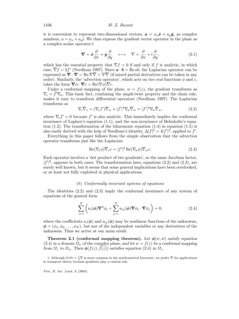
Figure 1. Conformal mapping, w = f(z), of a solution, φ, to a conformally invariantequation from a complicated domain, Ωz, and a simple domain, Ωw.

to ask whether any other equations share its conformal invariance, which is widelybelieved to be unique.

In this paper we show that certain systems of nonlinear equations, with non-harmonic solutions, are also conformally invariant. In § 2, we give a simple proof ofthis fact and some of its consequences. In § 3, we discuss applications to nonlineardiffusion phenomena and show that single conformally invariant equations can alwaysbe reduced to Laplace’s equation (which is not true for coupled systems). In § 4, weapply conformal mapping to nonlinear advection–diffusion in a potential flow, whichis equivalent to streamline coordinates in a special case (Boussinesq 1905). In § 5,we apply conformal mapping to nonlinear electrochemical transport, apparently forthe first time. In § 6, we summarize the main results. Applications to non-Laplacianfractal growth are a common theme throughout the paper (see §§ 2, 4 and 6).

2. Mathematical theory

(a) Conformal mapping without Laplace’s equation?

The standard application of conformal mapping is based on two facts.

(i) Any harmonic function, φ, in a singly connected planar domain, Ωw, is the realpart of an analytic function, Φ, the ‘complex potential’ (which is unique up toan additive constant): φ = Re Φ(w).

(ii) Since analyticity is preserved under composition, harmonicity is preservedunder conformal mapping, so φ = Re Φ(f(z)) is harmonic in Ωz = f−1(Ωw).

Presented like this, it seems that conformal mapping is closely tied to harmonic func-tions, but fact (ii) simply expresses the conformal invariance of Laplace’s equation:a solution, φ(w), is the same in any mapped coordinate system, φ(f(z)). Fact (i),a special relation between harmonic functions and analytic functions, is not reallyneeded. If another equation were also conformally invariant, then its non-harmonicsolutions, φ(w, w), would be preserved under conformal mapping in the same way,φ(f(z), f(z)) (see figure 1).

In order to seek such non-Laplacian invariant equations, we review the transfor-mation properties of some basic differential operators. Following Argand and Gauss,


1436 M. Z. Bazant

it is convenient to represent two-dimensional vectors, a = axx + ayy, as complexnumbers, a = ax + ayi. We thus express the gradient vector operator in the plane asa complex scalar operator:†

∇ = x∂

∂x+ y

∂

∂y←→ ∇ =

∂

∂x+ i

∂

∂y, (2.1)

which has the essential property that ∇f = 0 if and only if f is analytic, in whichcase, ∇f = 2f ′ (Needham 1997). Since a · b = Re ab, the Laplacian operator can beexpressed as ∇ · ∇ = Re ∇∇ = ∇∇ (if mixed partial derivatives can be taken in anyorder). Similarly, the ‘advection operator’, which acts on two real functions φ and c,takes the form ∇φ · ∇c = Re(∇φ)∇c.

Under a conformal mapping of the plane, w = f(z), the gradient transforms as∇z = f ′∇w. This basic fact, combining the ampli-twist property and the chain rule,makes it easy to transform differential operators (Needham 1997). The Laplaciantransforms as

∇z∇z = (∇zf′)∇w + |f ′|2∇w∇w = |f ′|2∇w∇w, (2.2)

where ∇zf′ = 0 because f ′ is also analytic. This immediately implies the conformal

invariance of Laplace’s equation (1.1), and the non-invariance of Helmholtz’s equa-tion (1.2). The transformation of the biharmonic equation (1.4) in equation (1.5) isalso easily derived with the help of Needham’s identity, ∆|f |2 = 4|f ′|2, applied to f ′.

Everything in this paper follows from the simple observation that the advectionoperator transforms just like the Laplacian:

Re(∇zφ)∇zc = |f ′|2 Re(∇wφ)∇wc. (2.3)

Each operator involves a ‘dot product of two gradients’, so the same Jacobian factor,|f ′|2, appears in both cases. The transformation laws, equations (2.2) and (2.3), aresurely well known, but it seems that some general implications have been overlooked,or at least not fully exploited in physical applications.

(b) Conformally invariant systems of equations

The identities (2.2) and (2.3) imply the conformal invariance of any system ofequations of the general form

N∑i=1

(ai(φ)∇2φi +

N∑j=i

aij(φ)∇φi · ∇φj

)= 0, (2.4)

where the coefficients ai(φ) and aij(φ) may be nonlinear functions of the unknowns,φ = (φ1, φ2, . . . , φN ), but not of the independent variables or any derivatives of theunknowns. Thus we arrive at our main result.

Theorem 2.1 (conformal mapping theorem). Let φ(w, w) satisfy equation(2.4) in a domain Ωw of the complex plane, and let w = f(z) be a conformal mappingfrom Ωz to Ωw. Then φ(f(z), f(z)) satisfies equation (2.4) in Ωz.

† Although ∂/∂z = 12∇ is more common in the mathematical literature, we prefer ∇ for applications

in transport theory because gradients play a central role.



Whenever the system (2.4) can be solved analytically in some simple domain, thetheorem produces a family of exact solutions for all topologically equivalent domains.Otherwise, it allows a convenient numerical solution to be mapped to more compli-cated domains of interest. This is an enormous simplification for free boundary prob-lems, where the solution in an evolving domain can be obtained by time-dependentconformal mapping to a single, static domain.

Conformal mapping is most useful when the boundary conditions are also invariant.Dirichlet (φi = const.) or Neumann (n · ∇φi = 0) conditions are typically assumed,but here we consider the straightforward generalizations

bi(φ) = 0 andN∑

j=1

bij(φ)(n · ∇φj)αi = 0, (2.5)

respectively, where bi(φ) and bij(φ) are nonlinear functions of the unknowns, αi isa constant, and n is the unit normal. The conformal invariance of the former isobvious, so we briefly consider the latter.

It is convenient to locally transform a vector field F along a given contour asF = tF , so that Re F and Im F are the projections onto the unit tangent, t = dz/|dz|,and the (right-handed) unit normal, n = −it, respectively. Since the tangent trans-forms as tw = tzf

′/|f ′|, and the gradient as ∇z = f ′∇w, we find that ∇z = |f ′|∇w.The invariance of equation (2.5) follows after taking the imaginary part on the bound-ary contour.

(c) Gradient-driven flux densities

Generalizing ∇φ for Laplacian problems, we define a ‘flux density’ for solutions ofequation (2.4) to be any quasilinear combination of gradients:

Fi =N∑

j=1

cij(φ)∇φj , (2.6)

where cij(φ) are nonlinear functions. The transformation rules above for the gradientapply more generally to any flux density:

Fz = f ′Fw and Fz = |f ′|Fw. (2.7)

These basic identities imply a curious geometrical equivalence between solutions todifferent conformally invariant systems.

Theorem 2.2 (equivalence theorem). Let φ(1) and φ(2) satisfy equations ofthe form (2.4) with corresponding flux densities F (1) and F (2) of the form (2.6). IfF

(1)z = aF

(2)z on a contour Cz for some complex constant a, then F

(1)w = aF

(2)w on

the image Cw = f(Cz) after a conformal mapping w = f(z).

An important corollary pertains to ‘similarity solutions’ of equations (2.4) and (2.5)in which certain variables φi involved in a flux density depend on only one Carte-sian coordinate, say Re w, after conformal mapping: φi = Gi(Re f(z)). (Our exam-ples below are mostly of this type.) Such special solutions share the same flux lines(level curves of Im f(z)) and iso-potentials (level curves of Re f(z)) in any geometry


1438 M. Z. Bazant

attainable by conformal mapping. They also share the same spatial distribution offlux density on an iso-potential, although the magnitudes generally differ.

An important physical quantity is the total normal flux through a contour, oftencalled the ‘Nusselt number’, Nu. For any contour C, we define a complex total flux

I(C) =∫

C

F |dz| =∫

C

F dz,

such that Re I(C) is the integrated tangential flux and Im I(C) = Nu(C). Fromequation (2.7) and dw = f ′ dz, we conclude that I(Cz) = I(Cw). Therefore, fluxintegrals can be calculated in any convenient geometry.

This basic fact has many applications. For example, if Fw is constant on a contourCw = f(Cz), then for any conformal mapping, we have I(Cz) = I(Cw) = (Cw)Fw,where (Cw) is simply the length of Cw. For fluxes driven by gradients of harmonicfunctions, this is the basis for the method of iterated conformal maps for DLA,in which the ‘harmonic measure’ for random growth events on a fractal cluster isreplaced by a uniform probability measure on the unit circle (Hastings & Levitov1998).

More generally, a non-harmonic probability measure for fractal growth can beconstructed for any flux law of the form (2.6) for fields satisfying equation (2.4).According to the results above, the growth probability is simply proportional to thenormal flux density on the unit circle for the same transport problem after conformalmapping to the exterior of the unit disc. A non-trivial example is given below in § 4 c.This allows the Hastings–Levitov method to be extended to a broad class of non-Laplacian fractal-growth processes (Bazant et al . 2003).

(d) Conformal mapping to curved surfaces

The conformal mapping theorem is even more general than it might appear fromour proof. The domain Ωz may be contained in any two-dimensional manifold. Thisbecomes clear from the recent work of Entov & Etingof (1991, 1997), who solvedviscous fingering problems on various curved surfaces by conformal mapping to thecomplex plane, e.g. via stereographic projection from the Riemann sphere. Theyexploited the fact that Laplace’s equation is invariant under any conformal mapping,w = f(z), from the plane to a curved surface because the Laplacian transforms as∇2

z = J∇2w, where J(f(z)) is the Jacobian. The system (2.4) shares this general

conformal invariance because the advection operator transforms in the same way,∇zφ·∇zc = J∇wφ·∇wc. The application of these ideas to non-Laplacian transport-limited growth phenomena on curved surfaces is work in progress with J. Choi andD. Crowdy; here we focus on conformal mappings in the plane, described by analyticfunctions.

3. Physical applications to diffusion phenomena

Conformally invariant boundary-value problems of the form (2.4) and (2.5) com-monly arise in physics from steady conservation laws,

∂ci

∂t= ∇ · Fi = 0, (3.1)



for gradient-driven flux densities (equation (2.6)) with algebraic (b(ci) = 0) or zero-flux (n · Fi = 0) boundary conditions, where ci is the concentration and Fi the fluxof substance i. Hereafter, we focus on flux densities of the form

Fi = ciui − Di(ci)∇ci, ui ∝ ∇φ, (3.2)

where Di(ci) is a nonlinear diffusivity, ui is an irrotational vector field causing advec-tion, and φ is a (possibly non-harmonic) potential. Examples include advection–diffusion in potential flows and bulk electrochemical transport.

Before discussing these cases of coupled dependent variables, it is instructive toconsider nonlinear diffusion in only one variable. The most general equation of thetype (2.4) for one variable is

a(c)∇2c = |∇c|2. (3.3)

This equation arises in the Stefan problem of dendritic solidification, where c is thedimensionless temperature of a supercooled melt and a(c) is Ivantsov’s function,which implicitly determines the position of the liquid–solid interface via a(c) = 1(Ivantsov 1947). In two dimensions, Bedia & Ben Amar (1994) prove the conformalinvariance of equation (3.3) and then study similarity solutions, c(ξ, η) = G(η), byconformal mapping, w = ξ + iη, to a plane of parallel flux lines:

a(G)G′′ = (G′)2, (3.4)

where an ordinary differential equation is solved.More generally, reversing these steps, it is straightforward to show that any mono-

tonic solution of equation (3.4) produces a nonlinear transformation c = G(φ) fromequation (3.3) to Laplace’s equation (1.1), which implies conformal invariance. Thereare several famous examples. For steady concentration-dependent diffusion,

∇ · (D(c)∇c) = 0, (3.5)

it is Kirchhoff’s transformation (Crank 1975): φ = G−1(c) =∫ c

0 D(x) dx. For Burg-ers’s equation in an irrotational flow (u = −∇h),

∂u

∂t+ λu · ∇u = ν∇2u, (3.6)

which is equivalent to the Kardar–Parisi–Zhang equation without noise (Kardar etal . 1986),

∂h

∂t= ν∇2h + 1

2λ|∇h|2, (3.7)

it is the Cole–Hopf transformation (Whitham 1974): φ = G−1(h) = eλh/2ν , whichyields the diffusion equation ∂φ/∂t = ν∇2φ, and thus Laplace’s equation in steadystate.

In summary, the general solutions to equation (3.3) are simply nonlinear functionsof harmonic functions, so, in the case of one variable, our theorems can be easilyunderstood in terms of standard conformal mapping. For two or more coupled vari-ables, however, this is no longer true, except for special similarity solutions. Thefollowing sections discuss some truly non-Laplacian physical problems.


1440 M. Z. Bazant

−1.5 −1.0 −0.5 0 0.5 1.0 1.5−0.5

0

0.5

1.0

1.5

2.0

0 0.1 0.2 0.3 0.4 0.5 0.6 0.7 0.8 0.9 −1.5 −1.0 −0.5 0 0.5 1.0 1.5

−1.5

−1.0

−0.5

0

0.5

1.0

1.5

−8 −6 −4 −2 0 2 4 6 8−8

−6

−4

−2

0

2

4

6

8

−5 −4 −3 −2 −1 0 1 2 3 4 5−5

−4

−3

−2

−1

0

1

2

3

4

5

−4 −3 −2 −1 0 1 2 3 4−4

−3

−2

−1

0

1

2

3

4

−1.5 −1.0 −0.5 0 0.5 1.0 1.5

−1.5

−1.0

−0.5

0

0.5

1.0

1.5

(e) ( f )

(a)

(b)

(c) (d )

Figure 2. Concentration profiles (contour plots) and potential-flow streamlines (yellow) forsteady, linear advection–diffusion layers around various absorbing surfaces (grey) at Pe = 1.All solutions are given by equation (4.3), where w = f(z) is a conformal map to the upperhalf-plane (a). The colour scale applies to all panels in figures 2 and 3.



−5 −4 −3 −2 −1 0 1 2 3 4 5−5

−4

−3

−2

−1

0

1

2

3

4

5

−5 −4 −3 −2 −1 0 1 2 3 4 5

(a) (b)

Figure 3. The steady linear advection–diffusion layer around a cylindrical rimon a flat plate at Pe = 0.1 (a) and Pe = 10 (b).

4. Steady advection–diffusion in a potential flow

We begin with a well-known system of the form (2.5), the only one to which conformalmapping has previously been applied (see below), albeit not in the present, more-general context. Consider the steady diffusion of particles or heat passively advectedin a potential flow, allowing for a concentration-dependent diffusivity. For a charac-teristic length L, speed U , concentration C, and diffusivity D(C), the dimensionlessequations are

∇2φ = 0 and Pe∇φ · ∇c = ∇ · (b(c)∇c), (4.1)where φ is the velocity potential (scaled to UL), c is the concentration (scaled to C),b(c) is the dimensionless diffusivity, and Pe = UL/D is the Peclet number. Thelatter equation is a steady conservation law for the dimensionless flux density, F =Pe c∇φ − b(c)∇c (scaled to DC/L). For b(c) = 1, these classical equations havebeen studied recently in two dimensions, e.g. in the contexts of tracer dispersion inporous media (Koplik et al . 1994, 1995), vorticity diffusion in strained wakes (Eames& Bush 1999; Hunt & Eames 2002), thermal advection–diffusion (Morega & Bejan1994; Sen & Yang 2000), and dendritic solidification in flowing melts (Kornev &Mukhamadullina 1994; Cummings et al . 1999).

(a) Similarity solutions for absorbing leading edges

Let us rederive a classical solution in the upper half-plane, w = ξ + iη (η > 0),which we will then map to other geometries. As shown in figure 2a, consider astraining velocity field, φ = Re Φ, Φ = w2, u = Φ′ = 2w = 2ξ − 2iη, which advects aconcentrated fluid, c(ξ,∞) = 1, toward an absorbing wall on the real axis, c(ξ, 0) = 0.Since the η-component of the velocity (toward the wall) is independent of ξ, as arethe boundary conditions, the concentration depends only on η. The scaling function,c(ξ, η; Pe) = S(

√Pe η) = S(η), satisfies

−2ηS′ = (b(S)S′)′, S(0) = 0, S(∞) = 1, (4.2)


1442 M. Z. Bazant

which is straightforward to solve, at least numerically. For b(S) = 1, equation (4.2)has a simple, analytical solution, S(η) = erf(η) (e.g. Cummings et al . 1999).

If extended to the entire w-plane, where two fluids of different concentrationsflow towards each other, this solution also describes a Burgers vortex sheet underuniform strain (Burgers 1948). In that case, (∂φ/∂ξ, ∂φ/∂η, c) plays the role of athree-dimensional velocity field satisfying the Navier–Stokes equations, and Pe playsthe role of the Reynolds number. Inserting a boundary, such as the stationary wall onthe real axis, however, is not consistent with Burgers’s solution because the no-slipcondition cannot be satisfied. The wall is crucial for conformal mapping to othergeometries because it enables singularities to be placed in the lower half-plane.

For every conformal map to the upper half-plane, w = f(z), we obtain a solution

φ = Re f(z)2 and c = S(√

Pe Im f(z)) for Im f(z) 0, (4.3)

which describes the nonlinear advection–diffusion layer in a potential flow of concen-trated fluid around the leading edge of an absorbing object. For a linear diffusivityS(η) = erf η, various examples are shown in figure 2. The choice f(z) =

√z − a in

part (c) describes a parabolic leading edge, x = (y/2α)2 − α2, where α = Im a 0.The limit of uniform flow past a half plate (a = 0) in part (b) is a special case thatis discussed below.

Another classical map, f(z) = zπ/(2π−β), describes a wedge of opening angle β,as shown in part (d) for β = π/2 (after a rotation by π/4). The half plate (β = 0)and the flat wall (β = π) discussed above are special cases. The diffusive flux on thesurface from equation (4.8), |∇φ| ∝

√Pe r−ν , is singular for acute angles β < π. The

geometry-dependent exponent ν = (π −β)/(2π −β) is the same for pure diffusion tothe wedge, φd ∝ Im f(z) (Barenblatt 1995). This insensitivity to Pe is a signature ofthe equivalence theorem, as explained below.

The less familiar mapping f(z) = z1/2 + z−1/2, which plays a crucial role innon-Laplacian growth problems (see below) places a cylindrical rim on the end ofa semi-infinite flat plate, as shown in part (e). The solution has a pleasing form inpolar coordinates:

φ =(

r +1r

)cos θ, (4.4)

c = erf[√

Pe

(√r − 1√

r

)sin 1

2θ

], (4.5)

where we have shifted the velocity potential, Φ = f(z)2 − 2 = z + z−1. Far from therim, we recover the half-plate similarity solution, since f(z) ∼

√z as |z| → ∞, but

close to the rim, as shown in figure 3, there is a non-trivial dependence on Pe. ForPe 1, a boundary layer of O(Pe−1/2) thickness forms on the front of the rim andextends to within a distance of O(Pe−1/2) from the rear stagnation point.

The flux density is easily calculated in the w-plane and then mapped to the z-planeusing equation (2.7):

Fz = 2f ′(z)f(z)Pe S(√

Pe Im f(z)) − f ′(z)√

Pe S′(√

Pe Im f(z)), (4.6)

where the first term describes advection and the second diffusion. The lines of advec-tive flux and diffusive flux, which are level curves of Im f(z)2 and Re f(z), respec-tively, are independent of Pe and b(c), as required by the equivalence theorem. In



particular, the diffusive flux lines have the same shape for any flow speed or nonlineardiffusivity, as in the case of simple linear diffusion (Pe = 0, b(c) = 1, c ∝ Im f(z)),even though advection and nonlinearity affect the lines of total flux.

The lines of total flux, called ‘heatlines’ in thermal advection–diffusion, are levelcurves of the ‘heat function’† (Kimura & Bejan 1983), which we define in complexnotation via ∇H = iF . For a linear diffusivity, we integrate equation (4.6) to obtainthe heat function for any conformal mapping:

H = 2 Re f(z)[Pe(Im f(z)) erf(

√Pe Im f(z)) +

√Pe

πexp(−Pe(Im f(z))2)

], (4.7)

which shows how the total-flux lines cross over smoothly from fluid streamlines out-side the diffusion layer (H ∼ Pe Im f(z)2, Pe Im f(z) 1) to diffusive-flux lines nearthe absorbing surface (H ∼ 2

√Pe/π Re f(z), Pe Im f(z) 1).

On the absorbing surface Im f(z) = 0, the flux density is purely diffusive and isin the normal direction. Its spatial distribution is determined geometrically by theconformal map,

|Fz| =√

Pe S′(0)|f ′(z)| on Im f(z) = 0, (4.8)

and only its magnitude depends on Pe, as predicted by the equivalence theorem. (Fora linear diffusivity, S′(0) = 2/

√π.) What appears to be the only previous result of this

kind is due to Koplik et al . (1994, 1995) in the context of tracer dispersion by linearadvection–diffusion in porous media. In the case of planar potential flow from a dipolesource to an equipotential absorbing sink, they proved that the spatial distributionof surface flux is independent of Pe. Here we see that the same conclusion holdsfor all similarity solutions to equation (4.1), even if (i) diffusive flux is not directedalong streamlines; (ii) the diffusivity is a nonlinear function of the concentration; and(iii) the domain is on a curved surface.

(b) Streamline coordinates

In proving their equivalence theorem, Koplik et al . (1994, 1995) transform equa-tion (4.1) in the linear case, b(c) = 1, to ‘streamline coordinates’:

Pe∂c

∂φ=

∂2c

∂φ2 +∂2c

∂ψ2 , (4.9)

where Φ = φ + iψ is the complex potential, φ is the velocity potential, and ψ isthe stream function. Because the independent and dependent variables are inter-changed, this is a type of hodographic transformation (Whitham 1974; Ben Amar &Poire 1999). The physical interpretation of equation (4.9) is that advection (the left-hand side) is directed along streamlines, while diffusion (the right-hand side) is alsoperpendicular to the streamlines, along iso-potential lines. In high-Reynolds-number

† Sen & Yang (2000) have recently shown that the heat function satisfies Laplace’s equation, ∇2H =0, in certain potential-dependent coordinates, ∇ ≡ e−Peφ∇. This might seem to be related to ourtheorems, but it does not provide a basis for conformal mapping of the domain because the coordinatetransformation is not analytic. Its value is also limited by the fact that the boundary conditions on H arenot known a priori. For example, on a surface where the concentration is specified, the unknown flux isalso required. These difficulties underscore the fact that the solutions of equation (4.1) are fundamentallynon-harmonic.


1444 M. Z. Bazant

fluid mechanics, this is a well-known trick due to Boussinesq (1905) that is still inuse today (Hunt & Eames 2002). Streamline coordinates are also used in Maksimov’smethod for dendritic solidification from a flowing melt (Cummings et al . 1999).

Boussinesq’s transformation is simply a conformal mapping to a geometry of uni-form flow. Any obstacles in the flow are mapped to line segments (branch cuts ofthe inverse map) parallel to the streamlines. Among the solutions (4.3), streamlinecoordinates correspond to the map f(z) =

√z from a plane of uniform flow past an

absorbing flat plate on the positive real axis (the branch cut), as shown in figure 2b.In this geometry, we have the boundary-value problem

Pe∂c

∂x= ∇2c, c(x > 0, 0) = 0, c(−∞, y) = 1,

which Carrier et al . (1983) have solved using the Wiener–Hopf technique. Moresimply, Greenspan has introduced parabolic coordinates (as in Greenspan 1961) toimmediately obtain the similarity solution derived above, c(x, y) = erf(

√Pe η), where

2η2 = −x +√

x2 + y2. The reason why this solution exists, however, only becomesclear after conformal mapping to non-streamline coordinates in the upper half-plane(see also Cummings et al . 1999).

As this example illustrates, streamline coordinates are not always convenient, soit is useful to exploit the possibility of conformal mapping to other geometries. Forsimilarity solutions, it is easier to work in a plane where the diffusive flux lines areparallel. Streamline coordinates are also often poorly suited to numerical methodsbecause stagnation points are associated with branch-point singularities. This is espe-cially problematic for free boundary problems: for flows toward infinite dendrites, itis easier to determine the evolving map from a half-plane (Cummings et al . 1999);for flows past finite growing objects, it is easier to map from the exterior of the unitcircle (Bazant et al . 2003).

(c) Non-similarity solutions for finite absorbing objects

It is tempting to try to eliminate the plate from the cylindrical rim in figure 3 byconformal mapping from the exterior of a finite object to the upper half-plane. Anysuch mapping in equation (4.3), however, requires a quadrupole point source of flow(mapped to ∞) on the object’s surface. This is illustrated in figure 2f by a Mobiustransformation from the exterior of the unit circle, f(z) = (1 + z)/i(1 − z), where asource at z = 1 ejects concentrated fluid in the +1 direction and sucks in fluid alongthe ±i directions. Thus we see that, due to the boundary conditions at ∞, uniformflow past an absorbing cylinder (or any other finite object) is in a different classof solutions, where the diffusive flux lines depend non-trivially on Pe. In streamlinecoordinates, this includes the problem of uniform flow past a finite absorbing strip,which requires solving Wijngaarden’s integral equation (Cummings et al . 1999).

Here, we study only the high-Pe asymptotics of advection–diffusion layers aroundfinite absorbing objects. Consider again the example of flow past a cylindrical rim ona flat plate (figure 3). Because disturbances in the concentration decay exponentiallyupstream beyond a distance of O(Pe−1/2), removing the plate on the downstreamside of the cylinder has no effect in the limit Pe → ∞, except on the plate itself(the branch cut), so the solution (4.4), (4.5) is also asymptotically valid near a finiteabsorbing cylinder (without the plate).



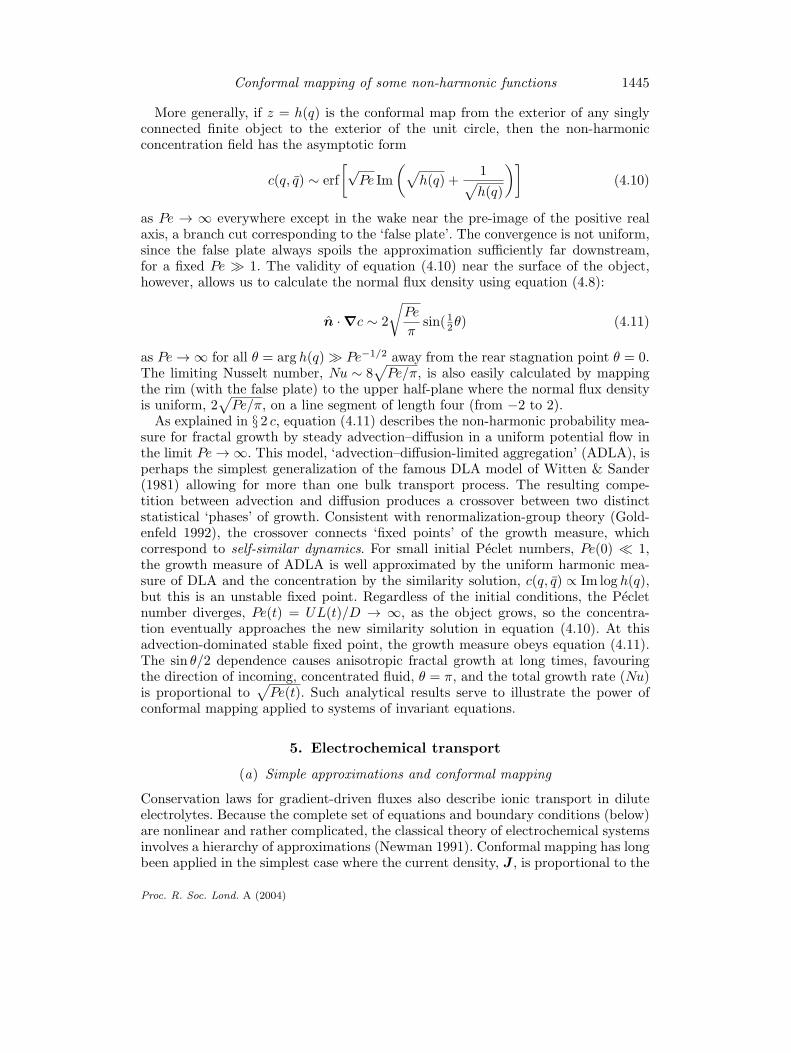
More generally, if z = h(q) is the conformal map from the exterior of any singlyconnected finite object to the exterior of the unit circle, then the non-harmonicconcentration field has the asymptotic form

c(q, q) ∼ erf[√

Pe Im(√

h(q) +1√h(q)

)](4.10)

as Pe → ∞ everywhere except in the wake near the pre-image of the positive realaxis, a branch cut corresponding to the ‘false plate’. The convergence is not uniform,since the false plate always spoils the approximation sufficiently far downstream,for a fixed Pe 1. The validity of equation (4.10) near the surface of the object,however, allows us to calculate the normal flux density using equation (4.8):

n · ∇c ∼ 2

√Pe

πsin(1

2θ) (4.11)

as Pe → ∞ for all θ = arg h(q) Pe−1/2 away from the rear stagnation point θ = 0.The limiting Nusselt number, Nu ∼ 8

√Pe/π, is also easily calculated by mapping

the rim (with the false plate) to the upper half-plane where the normal flux densityis uniform, 2

√Pe/π, on a line segment of length four (from −2 to 2).

As explained in § 2 c, equation (4.11) describes the non-harmonic probability mea-sure for fractal growth by steady advection–diffusion in a uniform potential flow inthe limit Pe → ∞. This model, ‘advection–diffusion-limited aggregation’ (ADLA), isperhaps the simplest generalization of the famous DLA model of Witten & Sander(1981) allowing for more than one bulk transport process. The resulting compe-tition between advection and diffusion produces a crossover between two distinctstatistical ‘phases’ of growth. Consistent with renormalization-group theory (Gold-enfeld 1992), the crossover connects ‘fixed points’ of the growth measure, whichcorrespond to self-similar dynamics. For small initial Peclet numbers, Pe(0) 1,the growth measure of ADLA is well approximated by the uniform harmonic mea-sure of DLA and the concentration by the similarity solution, c(q, q) ∝ Im log h(q),but this is an unstable fixed point. Regardless of the initial conditions, the Pecletnumber diverges, Pe(t) = UL(t)/D → ∞, as the object grows, so the concentra-tion eventually approaches the new similarity solution in equation (4.10). At thisadvection-dominated stable fixed point, the growth measure obeys equation (4.11).The sin θ/2 dependence causes anisotropic fractal growth at long times, favouringthe direction of incoming, concentrated fluid, θ = π, and the total growth rate (Nu)is proportional to

√Pe(t). Such analytical results serve to illustrate the power of

conformal mapping applied to systems of invariant equations.

5. Electrochemical transport

(a) Simple approximations and conformal mapping

Conservation laws for gradient-driven fluxes also describe ionic transport in diluteelectrolytes. Because the complete set of equations and boundary conditions (below)are nonlinear and rather complicated, the classical theory of electrochemical systemsinvolves a hierarchy of approximations (Newman 1991). Conformal mapping has longbeen applied in the simplest case where the current density, J , is proportional to the


1446 M. Z. Bazant

gradient of a harmonic function, φ, the electrostatic potential (Moulton 1905; Hineet al . 1956).

This approximation, the ‘primary current distribution’, describes the linearresponse of a homogeneous electrolyte to a small applied voltage or current, as well asmore general conduction in a supporting electrolyte (a great excess of inactive ions).The assumptions of Ohm’s law, J = σE = −σ∇φ (with a constant conductivity,σ), and no bulk charge sources or sinks, ∇ · J = 0, are analogous to those of poten-tial flow and incompressibility describe above. Each electrode is assumed to be anequipotential surface (see below), so the potential is simply that of a capacitor: har-monic with Dirichlet boundary conditions. Naturally, classical conformal mappingfrom electrostatics (Churchill & Brown 1990; Needham 1997) has been routinelyapplied, but it seems that conformal mapping has never been applied to any morerealistic models of electrochemical systems.

The ‘secondary current distribution’ introduces a kinetic boundary condition, n ·J = R(φ), which equates the normal current with a potential-dependent reactionrate, e.g. given by the Butler–Volmer equation (see below). In this case, conformalmapping could be of some use. Although the boundary condition acquires a non-constant coefficient, |f ′|, from equation (2.7), Laplace’s equation is preserved.

A more serious complication in the ‘tertiary current distribution’ is to allow thebulk ionic concentrations to vary in space (but not time). Ohm’s law is then replacedby a nonlinear current–voltage relation. Our main insight here is that conformalmapping can still be applied in the usual way, even though the equations are nonlinearand the potential is non-harmonic.

(b) Dilute-solution theory

In the usual case of a dilute electrolyte, the ionic concentrations, c1, c2, . . . , cN,and the electrostatic potential, φ, satisfy the Nernst–Planck equations (Newman1991), which have the form of equations (3.1) and (3.2), where the ‘advection’ veloc-ities, ui = −zieµi∇φ, are due to migration in the electric field, E = −∇φ. Here, zieis the charge (positive or negative) and µi the mobility of the ith ionic species. Thediffusivities are given by the Einstein relation, Di = kBTµi, where kB is Boltzmann’sconstant and T is the temperature. Scaling concentrations to a reference value, C,potential to the thermal voltage, kT/e, length to a typical electrode separation, L,and assuming that Di, T and ε are constants, the steady-state equations take thedimensionless form:

∇2ci + zi∇ · (ci∇φ) = 0. (5.1)

The ionic flux densities are Fi = −∇ci − zici∇φ (scaled to DiC/L).Because dissolved ions are very effective at charge screening, significant diffuse

charge can only exist in very thin (1–100 nm) interfacial double layers, where bound-ary conditions break the symmetry between opposite charge carriers. The ‘bulk’potential (outside the double layers) is then determined implicitly by the conditionof electroneutrality (Newman 1991),

N∑i=1

zici = 0,



which is trivially conformally invariant. Therefore, the most common model of steadyelectrochemical transport, equation (5.1), satisfies the assumptions of the confor-mal mapping theorem for any number of ionic species (N 2). Although the equa-tions differ from those of advection–diffusion in a potential flow, we can still mapto electric-field coordinates (the analogue of streamline coordinates), or any otherconvenient geometry.

Although the equations are conformally invariant, the boundary conditions are soonly in certain limits. General boundary conditions express mass conservation, eithern · Fi = 0 for an inert species or

n · ∇Fi = Ri(ci, φ) (5.2)

for an active species at an electrode, where Ri(ci, φ) is the Faradaic reaction-ratedensity (scaled to DiC/L). It is common to assume Arrhenius kinetics,

Ri(ci, φ) = k+cieziα+(φ−φe) − k−cre−ziα−(φ−φe), (5.3)

where k+ and k− are rate constants for deposition and dissolution, respectively(scaled to Di/L), α± are transfer coefficients, cr is the concentration of the reducedspecies (scaled to C), and φe is the electrode potential (scaled to kT/e). Taking diffuseinterfacial charge into account somewhat modifies R(ci, φ), but the basic structureof equation (5.2) is unchanged (Newman 1991; Bonnefont et al . 2001). Conformalmapping introduces a non-constant coefficient, |f ′|, in equation (5.2), but conformalinvariance is restored in the case of ‘fast reactions’ (k+ 1, k−cr 1), in whichequilibrium conditions prevail, R = 0, even during the passage of current. For asingle active species (say i = 1), the bulk potential at an electrode is then given bythe (dimensionless) Nernst equation:

φ − φe = ∆φeq = − log(kc1)z1(α+ + α−)

, (5.4)

where k = k+/k−cr is an equilibrium constant.†

(c) Conformal mapping with concentration polarization

The voltage across an electrochemical cell is conceptually divided into three parts(Newman 1991):

(i) the ‘ohmic polarization’ of the primary current distribution,

(ii) the ‘surface polarization’ of the secondary current distribution, and

(iii) ‘concentration polarization’, the remaining voltage attributed to bulk-concen-tration gradients.

Although concentration polarization can be significant, especially at large currentsin binary electrolytes, it is difficult to calculate. Analytical results are available onlyfor very simple geometries (mainly in one dimension), so our method easily producesnew results.

† Expressing equation (5.3) in terms of the ‘surface overpotential’, ηs = φ − φe − ∆φeq, yields themore familiar Butler–Volmer equation (Newman 1991).


1448 M. Z. Bazant

−0.8 −0.4 0 0.4 0.8

−0.8

−0.4

0

0.4

0.8

−3 −2 −1 0 1 2 3

−1.5

−1.0

−0.5

0

0.5

1.0

1.5

2.5 3.0 3.5 4.0 4.5 5.0

(a)

(b)

(c)

8 6 4 2 0 2 4 6 8

6

4

2

0

2

4

66

4

2

0

−2

−4

−6

6420−2−4−6 8−8

Figure 4. Similarity solutions for the electrostatic potential (contour plot) and current/electric-field lines (yellow) in a binary electrolyte at 90% of the limiting current (k = 1). Thesimple solution for parallel-plate electrodes (a) is conformally mapped to semi-infinite plates (b)and misaligned coaxial cylinders (c).

For example, consider a symmetric binary electrolyte (N = 2) of charge numberz = z+ = −z−, where the concentration, c = c+ = c−, and the potential satisfy

∇2c = 0 and ∇ · (c∇φ) = 0. (5.5)

(The concentrations are harmonic only for N = 2.) Assuming that anions are chemi-cally inert yields an invariant zero-flux condition at each electrode, n·(c∇φ−∇c) = 0,and (to break degeneracy) a constraint on the integral of c, which sets the total num-ber of anions (Bonnefont et al . 2001). In the limit of fast reactions, the bulk potentialat each electrode is given by the Nernst equation, φ = φe − log kc, where we scale φto kBT/ze and assume that α+ − α− = 1.

A class of similarity solutions is obtained by conformal mapping, w = f(z), to astrip, −1 < Im w < 1, representing parallel-plate electrodes, as shown in figure 4a.



We set φe = 0 at the cathode (Im w = −1) and φe = V , the applied voltage (inunits of kBT/ze), at the anode (Imw = 1). We then solve c′′ = 0 and (cφ′)′ = 0with appropriate boundary conditions to obtain a general solution for any conformalmapping to the strip:

c = 1 + J Im f(z), φ = log(

1 + J Im f(z)k(1 − J)2

), (5.6)

where J = tanh(V/4) is the uniform current density in the strip, scaled to its limitingvalue, Jlim = 2zeD+C/L. As J → 1, strong concentration polarization develops nearthe cathode, as shown in figure 4 for J = 0.9. At J = 1, the bulk concentration atthe cathode vanishes, and the cell voltage diverges due to diffusion limitation.

The classical conformal map, z = f−1(w) = πw + eπw (Churchill & Brown 1990),unfolds the strip like a ‘fan’ to cover the z-plane and maps the electrodes onto twohalf plates (Im z = ±π, Re z < −1). As shown in figure 4b, this solution describesthe fringe fields of semi-infinite, parallel-plate electrodes. The field and current linesare cycloids, za(η) = πa+iπη+eπaeiπη, as in the limit of a harmonic potential at lowcurrents, φ ∼ J Im f(z) − log k. At high currents, the magnitude of the electric fieldis greatly amplified near the cathode (the lower plate) by concentration polarization,but the shape of the field lines is always the same. This conclusion also holds forall other conformal mappings to the strip, such as the Mobius-log transformation,w = f(z) = i(1 + log(5z − 3)/(5 − 3z)), in figure 4c from the region between twonon-concentric circles.

It is interesting to note that the equivalence theorem applies to some physical situ-ations and not others. Similarity solutions like the ones above can only be derived fortwo equipotential electrodes by conformal mapping to a strip, where the current isuniform. In all such geometries, the electric field lines have the same shape as in theprimary current distribution. For three or more equipotential electrodes, however,this is no longer true because conformal mapping to the strip is topologically impos-sible, and thus similarity solutions do not exist. When the bulk potential varies atthe electrodes according to equation (5.2), the electric field lines generally differ fromboth the primary and secondary current distributions, even for just two electrodes.

6. Conclusion

We have observed that the nonlinear system of equations (2.4) involving ‘dot productsof two gradients’ is conformally invariant. This has allowed us to extend the classicaltechnique of conformal mapping to some non-harmonic functions arising in physics.Examples from transport theory are steady conservation laws for gradient-drivenfluxes (equation (3.2)). For one variable, the equations in our class (including somefamiliar examples in nonlinear diffusion) can always be reduced to Laplace’s equation.For two or more variables, the general solutions are not simply related to harmonicfunctions, but all similarity solutions exhibit an interesting geometrical equivalence.

For two variables, there is one example in our class, steady advection–diffusionin a potential flow, to which conformal mapping has previously been applied. Inthis case, our method is equivalent to Boussinesq’s streamline coordinates, but issomewhat more general. A nonlinear diffusivity is also allowed, and the mappingneed not be to a plane of uniform flow (parallel streamlines). In a series of examples,we have considered flows past absorbing leading edges and have generalized a recent


1450 M. Z. Bazant

equivalence theorem of Koplik et al . (1994, 1995). We have also considered the flowspast finite absorbing objects at high Peclet number.

Our class also contains the Nernst–Planck equations for steady, bulk electrochemi-cal transport, for which very few exact solutions are known in more than one dimen-sion. In electrochemistry, conformal mapping has been applied only to harmonicfunctions, so we have presented some new results, such as the concentration polariza-tions for semi-infinite, parallel-plate electrodes and for misaligned coaxial electrodes.More generally, we have shown that Ohm’s law gives the correct spatial distribution(but not the correct magnitude) of the electric field on any pair of equipotentialelectrodes in two dimensions, even if the transport is nonlinear and non-Laplacian,although this is not true for three or more electrodes. Such results could be usefulin modelling micro-electrochemical systems, where steady states are easily attained(due to short diffusion lengths) and quasi-planar geometries often arise.

As mentioned throughout the paper, our results can be applied to a broad classof moving free boundary problems for systems of non-Laplacian transport equations(Bazant et al . 2003). In contrast, the vast literature on conformal-map dynamics(cited in § 1) relies on complex-potential theory, which only applies to Laplaciantransport processes. Nevertheless, standard formulations—such as the Polubarinova–Galin equation for continuous Laplacian growth (Howison 1992) and the Hastings& Levitov (1998) method of iterated maps for DLA—can be easily generalized forcoupled non-Laplacian transport processes in our class. In the stochastic case, non-harmonic probability measures for fractal growth can be defined on any convenientcontour, such as the unit circle. As an example, we have derived the stable fixedpoint of the growth measure for an arbitrary absorbing object in a uniform back-ground potential flow (equation (4.11)). This sets the stage for conformal-mappingsimulations of ADLA, which might otherwise seem intractable.

The author is grateful to J. Choi for the colour figures; A. Ajdari, M. Ben Amar, J. Choi,K. Chu, D. Crowdy, B. Davidovitch, I. Eames, E. J. Hinch, H. K. Moffatt and A. Toomre forhelpful comments on the manuscript; MIT for a junior faculty leave; and ESPCI for hospitalityand support through the Paris Sciences Chair. This work was also supported by the MRSECProgram of the National Science Foundation under award number DMR 02-13282.

References

Ball, R. C. & Somfai, E. 2002 Theory of diffusion controlled growth. Phys. Rev. Lett. 89, 135503.Barenblatt, G. I. 1995 Scaling, self-similarity, and intermediate asymptotics. Cambridge Uni-

versity Press.Barra, F., Davidovitch, B. & Procaccia, I. 2002a Iterated conformal dynamics and Laplacian

growth. Phys. Rev. E65, 046144.Barra, F., Hentschel, H. G. E., Levermann, A. & Procaccia, I. 2002b Quasistatic fractures in

brittle media and iterated conformal maps. Phys. Rev. E65, 045101.Batchelor, G. K. 1967 An introduction to fluid dynamics. Cambridge University Press.Bazant, M. Z., Choi, J. & Davidovitch, B. 2003 Dynamics of conformal maps for a class of

non-Laplacian growth phenomena. Phys. Rev. Lett. 91, 045503.Bedia, M. A. & Ben Amar, M. 1994 Investigations of the dendrite problem at zero surface

tension in 2D and 3D geometries. Nonlinearity 7, 765–776.Ben Amar, M. 1991 Exact self-similar shapes in viscous fingering. Phys. Rev. A43, 5724–5727.Ben Amar, M. & Brener, E. 1996 Laplacian and diffusional growth: a unified theoretical descrip-

tion for symmetrical and parity-broken patterns. Physica D98, 128–138.



Ben Amar, M. & Poire, E. C. 1999 Pushing a non-Newtonian fluid in a Hele-Shaw cell: fromfingers to needles. Phys. Fluids 11, 1757–1767.

Bensimon, D., Kadanoff, L. P., Shraiman, B. I. & Tang, C. 1986 Viscous flows in two dimensionsRev. Mod. Phys. 58, 977–999.

Bonnefont, A., Argoul, F. & Bazant, M. Z. 2001 Asymptotic analysis of diffuse-layer effects ontime-dependent interfacial kinetics. J. Electroanalyt. Chem. 500, 52–61.

Boussinesq, M. J. 1905 Sur le pouvoir refroidissant d’un courant liquide ou gazeux. J. Math. 1,285–290.

Burgers, J. M. 1948 A mathematical model illustrating the theory of turbulence. Adv. Appl.Mech. 1, 171–199.

Carrier, G., Krook, M. & Pearson, C. E. 1983 Functions of a complex variable. Ithaca, NY: HodBooks.

Chan, R. H., Delillo,T. K. & Horn, M. A. 1997 Numerical solution of the biharmonic equationby conformal mapping. SIAM J. Sci. Comput. 18, 1571–1582.

Churchill, R. V. & Brown, J. W. 1990 Complex variables and applications, 5th edn. McGraw-Hill.Crank, J. 1975 Mathematics of diffusion, 2nd edn. Oxford: Clarendon.Crowdy, D. 1999 A note on viscous sintering and quadrature identities. Eur. J. Appl. Math. 10,

623–634.Crowdy, D. 2002 Exact solutions for the viscous sintering of multiply connected fluid domains.

J. Engng Math. 42, 225–242.Cummings, L. M., Hohlov, Y. E., Howison, S. D. & Kornev, K. 1999 Two-dimensional soldifi-

cation and melting in potential flows. J. Fluid Mech. 378, 1–18.Dai, W.-S., Kadanoff, L. P. & Zhou, S.-M. 1991 Interface dynamics and the motion of complex

singularities. Phys. Rev. A43, 6672–6682.Davidovitch, B., Hentschel, H. G. E., Olami, Z., Procaccia, I., Sander, L. M. & Somfai, E. 1999

DLA and iterated conformal maps. Phys. Rev. E59, 1368–1378.Davidovitch, B., Feigenbaum, M. J., Hentschel, H. G. E. & Procaccia, I. 2000 Conformal dynam-

ics of fractal growth patterns without randomness. Phys. Rev. E62, 1706–1715.Eames, I. & Bush, J. W. M. 1999 Long dispersion by bodies fixed in a potential flow. Proc. R.

Soc. Lond. A455, 3665–3686.Entov, V. M. & Etingof, P. I. 1991 Bubble contraction in Hele-Shaw cells. Q. J. Mech. Appl.

Math. 44, 507–535.Entov, V. M. & Etingof, P. I. 1997 Viscous flows with time-dependent free boundaries in a

non-planar Hele-Shaw cell. Eur. J. Appl. Math. 8, 23–35.Feigenbaum, M. J., Procaccia, I. & Davidovitch, B. 2001 Dynamics of finger formation in Lapla-

cian growth without surface tension. J. Stat. Phys. 103, 973–1007.Galin, L. A. 1945 Unsteady filtration with a free surface. Dokl. Akad. Nauk SSSR 47, 246–249.

(In Russian.)Goldenfeld, N. 1992 Lectures on phase transitions and the renormalization group. Reading, MA:

Perseus Books.Greenspan, H. P. 1961 On the flow of a viscous electrically conducting fluid. Q. Appl. Math. 18,

408–411.Hastings, M. B. 2001 Fractal to nonfractal phase transition in the dielectric breakdown model.

Phys. Rev. Lett. 87, 175502.Hastings, M. & Levitov, L. S. 1998 Laplacian growth as one-dimnesional turbulence. Physica

D116, 244–252.Hine, F., Yoshizawa, S. & Okada, S. 1956 Effects of walls of electrolytic cells on current distri-

bution. J. Electrochem. Soc. 103, 186–193.Howison, S. D. 1986 Fingering in Hele-Shaw cells. J. Fluid Mech. 167, 439–453.


1452 M. Z. Bazant

Howison, S. D. 1992 Complex variable methods in Hele-Shaw moving boundary problems. Eur.J. Appl. Math. 3, 209–224.

Hunt, J. C. R. & Eames, I. 2002 The disappearance of laminar and turbulent wakes in complexflows. J. Fluid Mech. 457, 111–132.

Ivantsov, G. P. 1947 Temperature field around spherical, cylindrical and needle-shaped crystalswhich grow in supercooled melts. Dokl. Akad. Nauk SSSR 58, 567–569. (In Russian.)

Kardar, M., Parisi, G. &. Zhang, Y.-C. 1986 Dynamic scaling of growing interfaces. Phys. Rev.Lett. 56, 889–892.

Kessler, D. A., Koplik, J. & Levine, H. 1988 Pattern selection in fingered growth phenomena.Adv. Phys. 37, 255–339.

Kimura, S. & Bejan, A. 1983 The ‘heatline’ visualization of convective heat transfer. J. HeatTransfer 105, 916–919.

Koplik, J., Redner, S. & Hinch, E. J. 1994 Tracer dispersion in planar multipole flows. Phys.Rev. E50, 4650–4667.

Koplik, J., Redner, S. & Hinch, E. J. 1995 Universal and nonuniversal first-passage propertiesof planar multipole flows. Phys. Rev. Lett. 74, 82–85.

Kornev, K. & Mukhamadullina, G. 1994 Mathematical theory of freezing for flow in porousmedia. Proc. R. Soc. Lond. A447, 281–297.

Morega, M. & Bejan, A. 1994 Heatline visualization of forced convection in porous media. Int.J. Heat Fluid Flow 36, 42–47.

Morse, P. M. & Feshbach, H. 1953 Methods of theoretical physics. McGraw-Hill.Moulton, H. F. 1905 Current flow in rectangular conductors. Proc. Lond. Math. Soc. 3, 104–110.Muskhelishvili, N. I. 1953 Some basic problems in the mathematical theory of elasticity. Gronin-

gen: Noordhoff.Needham, T. 1997 Visual complex analysis. Oxford: Clarendon Press.Newman, J. 1991 Electrochemical systems, 2nd edn. Englewood Cliffs, NJ: Prentice-Hall.Niemeyer, L., Pietronero, L. & Wiesmann, H. J. 1984 Fractal dimension of dielectric breakdown.

Phys. Rev. Lett. 52, 1033–1036.Polubarinova-Kochina, P. Ya. 1945a On a problem of the motion of the contour of a petroleum

shell. Dokl. Akad. Nauk SSSR 47, 254–257. (In Russian.)Polubarinova-Kochina, P. Ya. 1945b Concerning unsteady motions in the theory of filtration.

Prikl. Mat. Mech. 9, 79–90. (In Russian.)Saffman, P. G. 1986 Viscous fingering in Hele-Shaw cells. J. Fluid Mech. 173, 73–94.Saffman, P. G. & Taylor, G. I. 1958 The penetration of a fluid into a porous medium or Hele-

Shaw cell containing a more viscous liquid. Proc. R. Soc. Lond. A245, 312–329.Sen, M. & Yang, K. T. 2000 Laplace’s equation for convective scalar transport in potential flow.

Proc. R. Soc. Lond. A456, 3041–3045.Shraiman, B. I. & Bensimon, D. 1984 Singularities in nonlocal interface dynamics. Phys. Rev.

A30, 2840–2842.Somfai, E., Sander, L. M. & Ball, R. C. 1999 Scaling and crossovers in diffusion aggregation.

Phys. Rev. Lett. 83, 5523–5526.Stepanov, M. G. & Levitov, L. S. 2001 Laplacian growth with separately controlled noise and

anisotropy. Phys. Rev. E63, 061102.Tanveer, S. 1987 Analytical theory for the selection of a symmetrical Saffman–Taylor finger in

a Hele-Shaw cell. Phys. Fluids 30, 1589–1605.Tanveer, S. 1993 Evolution of Hele-Shaw interface for small surface tension. Phil. Trans. R. Soc.

Lond. A343, 155–204.Trefethen, L. N. 1986 Numerical conformal mapping. Amsterdam: North-Holland.Whitham, G. B. 1974 Linear and nonlinear waves. Wiley.Witten, T. A. & Sander, L. M. 1981 Diffusion-limited aggregation: a kinetic critical phenomenon.

Phys. Rev. Lett. 47, 1400–1403.


conformal mapping of some non-harmonic functions in transport theory...

Documents