conformal einstein spaces and bach tensor generalizations...
TRANSCRIPT
Linkoping Studies in Science and Technology. ThesesNo. 1113
Conformal Einstein spaces and Bach
tensor generalizations in n dimensions
Jonas Bergman
Matematiska institutionenLinkopings universitet, SE-581 83 Linkoping, Sweden
Linkoping 2004
August 20, 2004 (15:33)

ii
Conformal Einstein spaces andBach tensor generalizations in n dimensions
c© 2004 Jonas Bergman
Matematiska institutionenLinkopings universitetSE-581 83 Linkoping, [email protected]
LiU-TEK-LIC-2004:42ISBN 91-85295-28-0ISSN 0280-7971
Printed by UniTryck, Linkoping 2004
August 20, 2004 (15:33)
iii
Abstract
In this thesis we investigate necessary and sufficient conditions for an n-dimensional space, n ≥ 4, to be locally conformal to an Einstein space.After reviewing the classical results derived in tensors we consider thefour-dimensional spinor result of Kozameh, Newman and Tod. The in-volvement of the four-dimensional Bach tensor (which is divergence-freeand conformally well-behaved) in their result motivates a search for ann-dimensional generalization of the Bach tensor Bab with the same prop-erties. We strengthen a theorem due to Belfagon and Jaen and give a basis(Uab, V ab and W ab) for all n-dimensional symmetric, divergence-free 2-index tensors quadratic in the Riemann curvature tensor. We discover thesimple relationship Bab = 1
2Uab + 16V ab and show that the Bach tensor is
the unique tensor with these properties in four dimensions. Unfortunatelywe have to conclude, in general that there is no direct analogue in higherdimension with all these properties.Nevertheless, we are able to generalize the four-dimensional results due toKozameh, Newman and Tod to n dimensions. We show that a genericspace is conformal to an Einstein space if and only if there exists a vectorfield satisfying two conditions. The explicit use of dimensionally dependentidentities (some of which are newly derived in this thesis) is also exploitedin order to make the two conditions as simple as possible; explicit examplesare given in five and six dimensions using these tensor identities.For n dimensions, we define the tensors babc and Bab, and we show thattheir vanishing is a conformal invariant property which guarantees that thespace with non-degenerate Weyl tensor is a conformal Einstein space.
Acknowledgments
First and foremost, I would like to thank my supervisors Brian Edgar andMagnus Herberthson for their constant support, encouragement, and gen-erous knowledge sharing, and for all the interesting discussions, and forgiving me this chance to work on such an interesting topic.Thanks also goes to all my friends and colleagues at the Department ofMathematics, and especially Arne Enqvist for his support. I would alsolike to mention Anders Hoglund, who let me use his fantastic programTensign, and Ingemar and Goran, who read the manuscript and gave mevaluable comments. Thanks guys!Finally, but not least, I would like to thank Pauline and my family for theirsupport, encouragement, and understanding and for putting up with me,especially during the last month.
Jonas Bergman, Linkoping, 20 September 2004
August 20, 2004 (15:33)

iv
August 20, 2004 (15:33)
Contents
Abstract and Acknowledgments iii
Contents v
1 Introduction and outline of the thesis 1
2 Preliminaries 52.1 Conventions and notation . . . . . . . . . . . . . . . . . . . 52.2 Conformal transformations . . . . . . . . . . . . . . . . . . 82.3 Conformally flat spaces . . . . . . . . . . . . . . . . . . . . 10
3 Conformal Einstein equations and classical results 133.1 Einstein spaces . . . . . . . . . . . . . . . . . . . . . . . . . 133.2 Conformal Einstein spaces . . . . . . . . . . . . . . . . . . . 143.3 The classical results . . . . . . . . . . . . . . . . . . . . . . 15
4 The Bach tensor in four dimensions and possible general-izations 174.1 The Bach tensor in four dimensions . . . . . . . . . . . . . . 174.2 Attempts to find an n-dimensional Bach tensor . . . . . . . 204.3 The tensors Uab, Vab and Wab . . . . . . . . . . . . . . . . . 224.4 Four-dimensional Bach tensor expressed in Uab, Vab and Wab 274.5 An n-dimensional tensor expressed in Uab, Vab and Wab . . 28
5 The Kozameh-Newman-Tod four-dimensional result and theBach tensor 335.1 Two useful lemmas . . . . . . . . . . . . . . . . . . . . . . . 345.2 C-spaces and conformal C-spaces . . . . . . . . . . . . . . . 355.3 Conformal Einstein spaces . . . . . . . . . . . . . . . . . . . 385.4 J = 0 . . . . . . . . . . . . . . . . . . . . . . . . . . . . . . 40
6 Listing’s result in four dimensions 426.1 Non-degenerate Weyl tensor . . . . . . . . . . . . . . . . . . 426.2 Conformal C-spaces . . . . . . . . . . . . . . . . . . . . . . 436.3 Conformal Einstein spaces . . . . . . . . . . . . . . . . . . . 44
August 20, 2004 (15:33)
vi
7 Listing’s result in n dimensions 457.1 Non-degenerate Weyl tensor . . . . . . . . . . . . . . . . . . 457.2 Conformal C-spaces . . . . . . . . . . . . . . . . . . . . . . 467.3 Conformal Einstein spaces . . . . . . . . . . . . . . . . . . . 47
8 Edgar’s result in n dimensions 488.1 Using the Cayley-Hamilton Theorem . . . . . . . . . . . . . 48
Four dimensions . . . . . . . . . . . . . . . . . . . . . . . . 50Higher dimensions . . . . . . . . . . . . . . . . . . . . . . . 50
8.2 Using dimensionally dependent identities . . . . . . . . . . . 51A five-dimensional example . . . . . . . . . . . . . . . . . . 52Six-dimensional examples . . . . . . . . . . . . . . . . . . . 53
9 Generalizing the Bach tensor in n dimensions 559.1 A generic Weyl tensor . . . . . . . . . . . . . . . . . . . . . 559.2 The generalization of the KNT result . . . . . . . . . . . . . 569.3 n dimensions using generic results . . . . . . . . . . . . . . 599.4 Five-dimensional spaces using dimensional dependent iden-
tities . . . . . . . . . . . . . . . . . . . . . . . . . . . . . . . 609.5 Six-dimensional spaces using dimensional dependent identities 61
10 Conformal properties of different tensors 6210.1 The tensors babc and Bac and their conformal properties in
generic spaces . . . . . . . . . . . . . . . . . . . . . . . . . . 6210.2 The tensor Lab and its conformal properties . . . . . . . . . 65
11 Concluding remarks and future work 67
A The Cayley-Hamilton Theorem and the translation of theWeyl tensor/spinor to a matrix 69A.1 The Cayley-Hamilton Theorem . . . . . . . . . . . . . . . . 69
The case where n = 3 and the matrix is trace-free. . . . . . 70The case where n = 6 and the matrix is trace-free. . . . . . 71
A.2 Translation of Cabcd to a matrix CA
B . . . . . . . . . . . . 71A.3 Translation of ΨAB
CD to a matrix Ψ . . . . . . . . . . . . . 72
B Dimensionally dependent tensor identities 74B.1 Four-dimensional identities . . . . . . . . . . . . . . . . . . 74B.2 Five-dimensional identities . . . . . . . . . . . . . . . . . . . 75B.3 Six-dimensional identities . . . . . . . . . . . . . . . . . . . 76B.4 Lovelock’s quartic six-dimensional identity . . . . . . . . . . 77
C Weyl scalar invariants 79C.1 Weyl scalar invariants in 4 dimensions. . . . . . . . . . . . . 79
August 20, 2004 (15:33)

vii
D Computer tools 84D.1 GRTensor II . . . . . . . . . . . . . . . . . . . . . . . . . . . 84D.2 Tensign . . . . . . . . . . . . . . . . . . . . . . . . . . . . . 85
References 87
August 20, 2004 (15:33)

viii
August 20, 2004 (15:33)
Chapter 1
Introduction and outlineof the thesis
Within semi-Riemannian geometry there are classes of spaces which havespecial significance from geometrical and/or physical viewpoints; e.g., flatspaces with zero Riemann curvature tensor, conformally flat spaces (i.e.,spaces conformal to flat spaces) with Weyl tensor equal to zero, Einsteinspaces with trace-free Ricci tensor equal to zero. There are a number ofboth physical and geometrical reasons to study conformally Einstein spaces(i.e., spaces conformal to Einstein spaces), and it has been a long-standingclassical problem to find simple characterizations of these spaces in termsof the Riemann curvature tensor.Therefore, in this thesis, we will investigate necessary and sufficient con-ditions for an n-dimensional space, n ≥ 4, to be locally conformal to anEinstein space, a subject studied since the 1920s. Global properties willnot be considered here.The first results in this field are due to Brinkmann [6], [7], but also Schouten[36] has contributed to the subject; they both considered the general n-dimensional case. Nevertheless, the set of conditions they found is large,and not useful in practice.Later, in 1964, Szekeres [39] introduced spinor tools into the problem andproposed a partial solution in four dimensions using spinors, restrictingthe space to be Lorentzian, i.e., to have signature −2. Nevertheless, thespinor conditions he found are hard to analyse and complicated to translateinto tensors. Wunsch [43] pointed out a mistake in Szekeres’s paper whichmeans that his conditions are only necessary.However, in 1985, Kozameh, Newman and Tod [27] continued with thespinor approach and found a much simpler set consisting of only two in-dependent necessary and sufficient conditions for four-dimensional spaces;however, the price they paid for this simplicity was that the result was re-stricted to a subspace of the most general class of spaces − those for which
August 20, 2004 (15:33)

2
one of the scalar invariants of the Weyl tensor is non-zero, i.e.,
J =12
(Cab
cdCcd
efCefab − i∗Cab
cd∗Ccd
ef∗Cef
ab
)6= 0 . (1.1)
One of their conditions is the vanishing of the Bach tensor Bab; in fourdimensions this tensor has a number of nice properties.The condition J 6= 0 in the result of Kozameh et al. [27] has been relaxed,also using spinor methods, by Wunsch [43], [44], by adding a third conditionto the set found by Kozameh et al. This still leaves some spaces excluded;in particular the case when the space is of Petrov type N, although Czapor,McLenaghan and Wunsch [12] have some results in the right direction.The spinor formalism is the natural tool for general relativity in four dimen-sions in a Lorentzian space [32], [33] since it has built in both four dimen-sions and signature −2; on the other hand, it gives little guidance on howto generalize to n-dimensional semi-Riemannian spaces. However, using amore differential geometry point of view, Listing [28] recently generalizedthe result of Kozameh et al. [27] to n-dimensional semi-Riemannian spaceshaving non-degenerate Weyl tensor. Listing’s results have been extendedby Edgar [13] using the Cayley-Hamilton Theorem and dimensionally de-pendent identities [14], [29].There have been other approaches to this problem. For example, Kozameh,Newman and Nurowski [26] have interpreted and studied the necessaryand sufficient condition for a space to be conformal to an Einstein spacein terms of curvature restrictions for the corresponding Cartan conformalconnection. Also Baston and Mason [3], [4], working with a twistorialformulation of the Einstein equations, found a different set of necessaryand sufficient conditions. However, we shall restrict ourselves to a classicalsemi-Riemannian geometry approach.
In this thesis we are going to try and find n-dimensional tensors, n ≥ 4,generalizing the Bach tensor in such a way that as many good proper-ties of the four-dimensional Bach tensor as possible are carried over to then-dimensional generalization. We shall also investigate how these general-izations of the Bach tensor link up with conformal Einstein spaces.
The first part of this thesis will review the classical tensor results; Chapters5 to 8 will review and extend a number of the results in both spinorsand tensors during the last 20 years. In the remaining chapters we willpresent some new results and also discuss the directions where this workcan develop in the future. We have also included four appendices in whichwe have collected some old and developed some new results needed in thethesis, but to keep the presentation as clear as possible we have chosen tosummarize these at the end.
The outline of the thesis is as follows:
We begin in Chapter 2 by fixing the conventions and notation used in thethesis and giving some useful relations and identities. The chapter ends by
August 20, 2004 (15:33)

3
reviewing and proving the classical result that a space is conformally flatif and only if the Weyl tensor is identically zero.In Chapter 3 Einstein spaces and conformal Einstein spaces are introducedand the conformal Einstein equations are derived. Some of the earlierresults in the field are also mentioned.In Chapter 4 the Bach tensor Bab in four dimensions is defined and var-ious attempts to find an n-dimensional counterpart are investigated. Westrengthen a theorem due to Belfagon and Jean and give a basis (Uab, V ab
and W ab) for all n-dimensional symmetric, divergence-free 2-index tensorsquadratic in the Riemann curvature tensor. We discover the simple rela-tionship Bab = 1
2Uab + 16V ab between the four-dimensional Bach tensor
and these tensors, and show that this is the only 2-index tensor (up toconstant rescaling) which in four dimensions is symmetric, divergence-freeand quadratic in the Riemann curvature tensor. We also demonstrate thatthere is no useful analogue in higher dimensions.Chapter 5 deals with the four-dimensional result for spaces in which J 6= 0due to Kozameh, Newman and Tod, and both explicit and implicit resultsin their paper are proven and discussed. We also explore a little furtherthe relationship between spinor and tensor results.In Chapter 6 and Chapter 7 the recent work of Listing in spaces withnon-degenerate Weyl tensors is reviewed; Chapter 6 deals with the four-dimensional case and Chapter 7 with the n-dimensional case.In Chapter 8 we look at the extension of Listing’s result due to Edgar usingthe Cayley-Hamilton Theorem and dimensionally dependent identities.In Chapter 9 the concept of a generic Weyl tensor and a generic spaceis defined. The results of Kozameh, Newman and Tod are generalizedand generic results presented. We show that an n-dimensional genericspace is conformal to an Einstein space if and only if there exists a vectorfield satisfying two conditions. The explicit use of dimensionally dependentidentities is also exploited in order to make these two conditions as simpleas possible; explicit examples are given in five and six dimensions.In Chapter 10, for n dimensions, we define the tensors babc and Bab, whosevanishing guarantees a space with non-degenerate Weyl tensor being aconformal Einstein space. We show that babc is conformally invariant inall spaces with non-degenerate Weyl tensor, and that Bab is conformallyweighted with weight −2, but only in spaces with non-degenerate Weyl ten-sor where babc = 0. We also show that the Listing tensor Lab is conformallyinvariant in all n-dimensional spaces with non-degenerate Wely tensor.In the final chapter we briefly summarize the thesis and discuss differentways of continuing this work and possible applications of the results givenin the earlier chapters.Appendix A deals with the representations of the Weyl spinor/tensor asmatrices and discusses the Cayley-Hamilton Theorem for matrices and ten-sors.In Appendix B dimensionally dependent identities are discussed. A number
August 20, 2004 (15:33)

4
of new tensor identities in five and six dimensions suitable for our purposeare derived; these identities are exploited in Chapter 9.In Appendix C, in four dimensions, we look at the Weyl scalar invariantsand derive relations between the two complex invariants naturally arisingfrom spinors and the standard four real tensor invariants.The last appendix briefly comments on the computer tools used for someof the calculations in this thesis.
At an early stage of this investigation we became aware of the work of List-ing [28], who had also been motivated to generalize the work of Kozamehet al. [27]. So, although we had already anticipated some of the Listing’sgeneralizations independently, we have reviewed these generalizations aspart of his work in Chapters 6 and 7.
When we were writing up this thesis (May 2004) a preprint by Gover andNurowski [16] appeared on the http://arxiv.org/ . The first part of thispreprint obtains some of the results which we have obtained in Chapter 9in essentially the same manner; however, they do not make the link withdimensionally dependent identities, which we believe makes these resultsmore useful. The second part of this preprint deals with conformally Ein-stein spaces in a different manner based on the tractor calculus associatedwith the normal Cartan bundle. Out of this treatment emerges the resultson the conformal behavior of babc and Bac, which we obtained in a moredirect manner in Chapter 10. Due to the very recent appearance of [16] wehave not referred to this preprint in our thesis, since all of our work wasdone completely independently of it.
August 20, 2004 (15:33)

Chapter 2
Preliminaries
In this chapter we will briefly describe the notation and conventions usedin this thesis, but for a more detailed description we refer to [32] and [33].We also review and prove the classical result that a space is conformallyflat if and only if the Weyl tensor of the space is identically zero.
2.1 Conventions and notation
All manifolds we consider are assumed to be differentiable and equippedwith a symmetric non-degenerate bilinear form gab = gba, i.e. a met-ric. No assumption is imposed on the signature of the metric unless ex-plicitly stated, and we will be considering semi-Riemannian (or pseudo-Riemannian) spaces in general; we will on occasions specialize to (proper)Riemannian spaces (metrics with positive definite signature) and Lorentzianspaces (metrics with signature (+− . . .−)).
All connections, ∇, are assumed to be Levi-Civita, i.e. metric compatible,and torsion-free, e.g. ∇agbc = 0, and
(∇a∇b − ∇b∇a
)f = 0 for all scalar
fields f , respectively.
Whenever tensors are used we will use the abstract index notation, see [32],and when spinors are used we again follow the conventions in [32].
The Riemann curvature tensor is constructed from second order derivativesof the metric but can equivalently be defined as the four-index tensor fieldRabcd satisfying
2∇[a∇b]ωc = ∇a∇bωc −∇b∇aωc = −Rabcdωd (2.1)
for all covector fields ωa, and it has the following algebraic properties,Rabcd = R[ab][cd] = Rcdab; it satisfies the first Bianchi identity, R[abc]d = 0,and it also satisfies the second Bianchi identity, ∇[aRbc]de = 0.
August 20, 2004 (15:33)

6
From the Riemann curvature tensor (2.1) we define the Ricci (curvature)tensor, Rab, by the contraction
Rab = Racbc (2.2)
and the Ricci scalar, R, from the contracted Ricci tensor
R = Raa = Rab
ab . (2.3)
For dimensions n ≥ 3 the Weyl (curvature) tensor or the Weyl conformaltensor, Cabcd, is defined as the trace-free part of the Riemann curvaturetensor,
Cabcd = Rabcd− 2n− 2
(ga[cRd]b−gb[cRd]a
)+
2(n− 1)(n− 2)
Rga[cgd]b (2.4)
and as is obvious from above when Rab = 0 the Riemann curvature tensorreduces to the Weyl tensor. The Weyl tensor has all the algebraic propertiesof the Riemann curvature tensor, i.e. Cabcd = C [ab][cd] = Ccdab, Ca[bcd] = 0,and in addition is trace-free, i.e. Cabc
a = 0. It is also well known that theWeyl tensor is identically zero in three dimensions.
For clarity we note that due to our convention in defining the Riemanncurvature tensor (2.1) we have for an arbitrary tensor field Hb...d
f...h that(∇i∇j −∇j∇i
)Hb...d
f...h = Rijb0bHb0...d
f...h + . . . + Rijd0dHb...d0
f...h
−Rijff0Hb...d
f0...h − . . .−Rijhh0Hb...d
f...h0
(2.5)
and (2.5) is sometimes referred to as the Ricci identity.
We will use both the conventions in the literature for denoting covariantderivatives, e.g., both the “nabla” and the semicolon, ∇av ≡ v;a. Notehowever the difference in order of the indices in each case, ∇a∇bv ≡ v;ba.
For future reference we write out the twice contracted (second) Bianchiidentity,
∇aRab − 12∇bR = 0 , (2.6)
the second Bianchi identity in terms of the Weyl tensor
0 = Rab[cd;e] = Cab[cd;e] +1
(n− 3)ga[cCde]b
f;f +
1(n− 3)
gb[cCed]af;f ,
(2.7)the second contracted Bianchi identity for the Weyl tensor,
∇dCabcd =
(n− 3)(n− 2)
(− 2∇[aRb]c +
1(n− 1)
gc[b∇a]R)
. (2.8)
August 20, 2004 (15:33)
7
Note that (2.8) also can be written
∇dCabcd = − (n− 3)
(n− 2)Ccba (2.9)
where Cabc =(− 2∇[aRb]c + 1
(n−1)gc[b∇a]R)
is the Cotton tensor. TheCotton tensor plays an important role in the study of thee-dimensionalspaces [5] ,[15], [21].
We also have the divergence of (2.8)
Cabcd;db =
(n− 3)(n− 2)
Rac;bb − (n− 3)
2(n− 1)R;ac +
(n− 3)n(n− 2)2
RabRbc
− (n− 3)(n− 2)
RbdCabcd − (n− 3)(n− 2)2
gacRbdRbd
− n(n− 3)(n− 1)(n− 2)2
RRac − (n− 3)2(n− 1)(n− 2)
gacR;bb
+(n− 3)
(n− 1)(n− 2)2gacR
2 . (2.10)
Using the second Bianchi identity for the Weyl tensor, the Ricci identityand finally decomposing the Riemann tensor into the Weyl tensor, the Riccitensor and the Ricci scalar we get the following identity
∇[e∇dCab]cd =(n− 3)(n− 2)
R[ab|c|fRe]f =(n− 3)(n− 2)
C [ab|c|fRe]f . (2.11)
In an n-dimensional space, letting HΩa1...ap = HΩ
[a1...ap] denote anytensor with an arbitrary number of indices schematically denoted by Ω,plus a set of p ≤ n completely antisymmetric indices a1 . . . ap, we define
the (Hodge) dual∗HΩ
ap+1...an with respect to a1 . . . ap by
∗HΩ
ap+1...an =1p!
ηa1...anHΩa1...ap (2.12)
where η is the totally antisymmetric normalized tensor. Sometimes the ∗ isplaced over the indices onto which the operation acts, e.g. HΩ ∗
ap+1...an.
In the special case of taking the dual of a double two-form Habcd = H [ab][cd]
in four dimensions there are two ways to perform the dual operation; eitheracting on the first pair of indices, or the second pair. To separate the twowe define the left dual and the the right dual as
∗Hijcd =
12ηabijH
abcd (2.13)
August 20, 2004 (15:33)

8
and
H∗abij =
12ηcdijH
abcd (2.14)
respectively.
We are going to encounter highly structured products of Weyl tensors andto get a neater notation we follow [42] and make the following definition:
Definition 2.1.1. For a trace-free (2, 2)-form T abcd, i.e. for a tensor suchthat
T abad = 0 , T abcd = T [ab]cd = T ab[cd] (2.15)
an expression of the form
T abc1d1T
c1d1c2d2 . . . T cm−2dm−2
cm−1dm−1Tcm−1dm−1
ef︸ ︷︷ ︸m
(2.16)
where the indices a, b, e and f are free, is called a chain (of the zeroth kind)of length m and is written1 T [m]ab
ef .
Hence, we have for instance that C[3]abcd = Cab
ijCij
klCkl
cd.
On occasions we will use matrices and these will always be written in boldcapital letters, e.g. A. In this context O and I will denote the zero- and theidentity matrix respectively and we will use square brackets to representthe operation of taking the trace of a matrix, e.g. [A] means the trace ofthe matrix A.
Throughout this thesis we will only be considering spaces of dimensionn ≥ 4. This is because in two dimensions all spaces are Einstein spaces andin three dimensions all spaces are conformally flat.
2.2 Conformal transformations
Definition 2.2.1. Two metrics gab and gab are said to be conformallyrelated if there exists a smooth scalar field Ω > 0 such that
gab = Ω2gab (2.17)
holds.
The metric gab is said to arise from a conformal transformation of gab.Clearly we have gab = Ω−2gab, since then gabgbc = gabgbc = δa
c .
1In [42] this is denoted T0[m]ab
ef .
August 20, 2004 (15:33)
9
To the rescaled metric gab there is a unique symmetric connection, ∇, com-patible with gab, i.e. ∇cgab = 0. The relation between the two connectionscan be found in [32] and acting on an arbitrary tensor field Hb...d
f...h it is
∇aHb...df...h =∇aHb...d
f...h + Qab0bHb0...d
f...h + . . . + Qad0dHb...d0
f...h
−Qaff0Hb...d
f0...h − . . .−Qahh0Hb...d
f...h0 (2.18)
withQab
c = 2Υ(aδcb) − gabΥc (2.19)
where Υa = Ω−1∇aΩ = ∇a(lnΩ) and Υa = gabΥb.
The relations between the tensors defined in (2.1) - (2.4) and their hattedcounterparts, i.e. the ones constructed from gab, are2
Rabcd =Rabc
d − 2δd[a∇b]Υc + 2gc[a∇b]Υd − 2δd
[bΥa]Υc
+ 2Υ[agb]cΥd + 2gc[aδdb]ΥeΥe , (2.20)
Rab = Rab + (n− 2)∇aΥb + gab∇cΥc
−(n− 2)ΥaΥb + (n− 2)gabΥcΥc , (2.21)
R = Ω−2(R + 2(n− 1)∇cΥc + (n− 1)(n− 2)ΥcΥc
), (2.22)
andCabc
d = Cabcd . (2.23)
Note that the positions of the indices in all equations (2.20) - (2.23) arecrucial since we raise and lower indices with different metrics, e.g. Cabcd =gdeCabc
e = Ω2gdeCabce = Ω2Cabcd.
Definition 2.2.2. A tensor field Hb...df...h is said to be conformally well-
behaved or conformally weighted (with weight ω) if under the conformaltransformation (2.17), gab = Ω2gab, there is a real number w such that
Hb...df...h → Hb...d
f...h = ΩωHb...df...h . (2.24)
If ω = 0 then Hb...df...h is said to be conformally invariant.
Following [32] we introduce the tensor
Pab = − 1(n− 2)
Rab +1
2(n− 1)(n− 2)Rgab (2.25)
2These can be found, for instance, in [40], but note that Wald is using a differentdefinition than (2.1) to define the Riemann curvature tensor.
August 20, 2004 (15:33)
10
and with the notation (2.25) we can express (2.2) - (2.4) as
Cabcd = Rab
cd + 4P [a[cgb]
d] , (2.26)
Rab = −(n− 2)P ab − gabP cc , (2.27)
andR = −2(n− 1)P c
c = −2(n− 1)P . (2.28)
The contracted second Bianchi identity for the Weyl tensor (2.8) can nowbe written
∇dCabcd = 2(n− 3)∇[aP b]c . (2.29)
Note that Pab is essentially Rab with a different trace term added and thatP ab simply replaces Rab to make equations such as (2.26) and (2.29) simplerthan (2.4) and (2.8), and hence to make calculations simpler. Furthermore,under a conformal transformation,
Pab = P ab + ΥaΥb −∇aΥb − 12gabΥcΥc , (2.30)
and
P = Ω−2(P −∇cΥc − (n− 2)
2ΥcΥc
), (2.31)
which are simpler than the corresponding equations (2.21) and (2.22).
2.3 Conformally flat spaces
Definition 2.3.1. A space is called flat if its Riemann curvature tensorvanishes, Rabcd = 0.
Since flat spaces are well understood we would like a simple condition on thegeometry telling us when there exists a conformal transformation makingthe space flat. Hence we define,
Definition 2.3.2. A space is called conformally flat if there exists a con-formal transformation gab = Ω2gab such that the Riemann curvature tensorin the space with metric gab vanishes, i.e., Rabcd = 0.
From (2.20) we know that a space is conformally flat if and only if
0 =Rabcd − 2δd
[a∇b]Υc + 2gc[a∇b]Υd − 2δd[bΥa]Υc
+ 2Υ[agb]cΥd + 2gc[aδdb]ΥeΥe (2.32)
for some gradient vector field Υa. Raising one index in equation (2.32) wecan rewrite this as
0 = Rabcd + 4δ
[c[a∇b]Υd] + 4Υ[aδ
[cb]Υ
d] + 2δ[c[aδ
d]b] ΥeΥe
= Rabcd + 4P [a
[cδd]b] (2.33)
August 20, 2004 (15:33)

11
where from (2.30) with Pab = 0 we have
P ab = ∇aΥb −ΥaΥb +12gabΥcΥc (2.34)
andP [ab] = 0 . (2.35)
We will now prove the important classical theorem3
Theorem 2.3.1. A space is conformally flat if and only if its Weyl tensoris zero.
Proof. The necessary part follows immediately from the conformal proper-ties of the Weyl tensor (2.23).
To prove the sufficient part we break up the proof into two steps. First weshall show that if there exists some symmetric 2-tensor P ab in a space suchthat
0 = Rabcd + 4P [a
[cδd]b] (2.36)
P ab = ∇aKb −KaKb +12gabKcK
c; P [ab] = 0 (2.37)
for some vector field Ka, then the space is conformally flat.
From (2.37) it follows that ∇[aKb] = 0 which means that locally Ka is agradient vector field,
Ka = ∇aΦ (2.38)
for some scalar field Φ, and substitution of P ab in (2.37) with this gradientexpression for Ka into (2.36) gives
0 =Rabcd − 2δd
[a∇b]∇cΦ + 2gc[a∇b]∇dΦ− 2δd[b
(∇a]Φ)∇cΦ
+ 2(∇[aΦ
)gb]c∇dΦ + 2gc[aδd
b]
(∇eΦ)∇eΦ ,
i.e., (2.20) with Υa = ∇aΦ, which implies that Rabcd = 0 and so the spaceis conformally flat, g = e2Φgab.
Secondly we shall show that if Cabcd = 0 then (2.36) and (2.37) are satisfied.From (2.26) it follows immediately that if Cabcd = 0,
0 = Rabcd + 4P [a
[cδd]b] (2.39)
3The necessary part is originally due to Weyl [41], and the sufficient part to Schouten[37].
August 20, 2004 (15:33)
12
i.e. (2.36) is satisfied. Also, if Cabcd = 0, we know from the second Bianchiidentity (2.29) that
∇[aP b]c = 0 . (2.40)
To check if (2.37) can be satisfied we calculate the integrability conditionof (2.37) which is
0 = ∇[cP a]b −∇[c∇a]Υb + Υb∇[cΥa] + Υ[a∇c]Υb −Υegb[a∇c]Υe
= ∇[cP a]b +(1
2Rca
be + 2P [c[bδ
e]a]
)Υe (2.41)
But from (2.39) and (2.40) it follows that this condition is identically sat-isfied. Hence we conclude that (2.37) is a consequence of (2.36).
To summarize, we have shown that Cabcd = 0 implies (2.36), which in turnimplies (2.36) and (2.37) (with the help of the Bianchi identities), meaningthat the space is conformally flat.
August 20, 2004 (15:33)
Chapter 3
Conformal Einsteinequations and classicalresults
In this chapter we will define conformal Einstein spaces and derive theconformal Einstein equations in n dimensions. We will also give a shortsummary of the classical results due to Brinkmann [6] and Schouten [36].
3.1 Einstein spaces
Definition 3.1.1. An n-dimensional space is said to be an Einstein spaceif the trace-free part of the Ricci tensor is identically zero, i.e.
Rab − 1n
gabR = 0 . (3.1)
Expressing this condition using the P ab tensor we get an expression havingthe same algebraic structure
(n− 2)(P ab − 1
ngabP
)= 0 , (3.2)
and we also note that in an Einstein space (2.25) becomes
P ab = − 12n(n− 1)
gabR . (3.3)
From the contracted Bianchi identity (2.6) we find for an Einstein spacethat
0 = 2∇aRab −∇bR = − (n− 2)n
∇bR , (3.4)
i.e. the Ricci scalar must be constant.
August 20, 2004 (15:33)

14
3.2 Conformal Einstein spaces
Definition 3.2.1. An n-dimensional space with metric gab is a confor-mal Einstein space (or conformally Einstein) if there exists a conformaltransformation gab = Ω2gab such that in the conformal space with metricgab
Rab − 1n
gabR = 0 , (3.5)
or equivalently
Pab − 1n
gabP = 0 . (3.6)
Note that from (2.22) and (3.4) we have that
R = Ω−2(R + 2(n− 1)∇cΥc + (n− 1)(n− 2)ΥcΥc
)= constant , (3.7)
where we used the notation introduced in Chapter 2.2. Further, equation(3.5) is equivalent to
Rab − 1n
gabR + (n− 2)∇aΥb − (n− 2)n
gab∇cΥc
− (n− 2)ΥaΥb +(n− 2)
ngabΥcΥc = 0 , (3.8)
and (3.6) to
P ab − 1n
gabP −∇aΥb +1n
gab∇cΥc + ΥaΥb − 1n
gabΥcΥc = 0 (3.9)
respectively. (3.8) or (3.9) is often referred to as the (n-dimensional) con-formal Einstein equations.
Taking a derivative of (3.7) gives the relations
0 = ∇aR− 2RΥa − 4(n− 1)Υa∇cΥc − 2(n− 1)(n− 2)ΥaΥcΥc
+ 2(n− 1)∇a∇cΥc + 2(n− 1)(n− 2)Υc∇aΥc
= ∇aP − 2PΥa + 2Υa∇cΥc + (n− 2)ΥaΥcΥc −∇a∇cΥc
− (n− 2)Υc∇aΥc (3.10)
and using this, the first integrability condition of (3.9) is calculated to be
∇[aPb]c +12CabcdΥd = 0 , (3.11)
or, using (2.29),
∇dCabcd + (n− 3)ΥdCabcd = 0 . (3.12)
Taking another derivative and using (2.29) again we have
∇b∇[aPb]c +12P bdCabcd + (n− 4)Υb∇[aPb]c = 0 (3.13)
August 20, 2004 (15:33)

15
and clearly both (3.11) and (3.13) are necessary conditions for a spaceto be conformally Einstein. Obviously we could get additional necessaryconditions by taking higher derivatives.
The last equation (3.13) can also be written
∇b∇dCabcd − (n− 3)(n− 2)
RbdCabcd − (n− 3)(n− 4)ΥbΥdCabcd = 0 (3.14)
and in dimension n = 4 this condition (3.14) reduces to a condition onlyon the geometry, and is independent of Υa. This condition,
Bac ≡ ∇b∇dCabcd − 12RbdCabcd = 0 , (3.15)
is a necessary, but not a sufficient, condition for a four-dimensional spaceto be conformally Einstein.
Note that if (3.8) holds for any vector field Ka,
Rab − 1n
gabR + (n− 2)KaKb − (n− 2)n
gab∇cKc
− (n− 2)KaKb +(n− 2)
ngabKcK
c = 0 , (3.16)
and remembering that Rab is symmetric, then by antisymmetrising we get∇[aKb] = 0, i.e. that Ka is locally a gradient. Hence we have that a spaceis locally a conformal Einstein space if and only if (3.16) holds for somevector field Ka. Given that P ab is defined by (2.25) this same statementalso holds for
P ab − 1n
gabP −∇aKb +1n
gab∇cKc + KaKb − 1
ngabKcK
c = 0 . (3.17)
3.3 The classical results
In 1924 Brinkmann [6] found necessary and sufficient conditions for a spaceto be conformally Einstein. In his approach he derived a large set of differ-ential equations involving Υa and by exploiting both existence and compat-ibility of this derived set he was able to formulate necessary and sufficientconditions. However, from his results it is hard to get a constructive set ofnecessary and sufficient conditions, and his results are not very useful inpractice.
Brinkmann later also studied in detail some special cases of conformal Ein-stein spaces [7].
August 20, 2004 (15:33)
16
Schouten [36] used a slightly different approach and looked directly at theexplicit form of integrability condition for the conformal Einstein equations,but he did not go beyond Brinkmann’s results as regards sufficient condi-tions. Schouten found the necessary condition (3.13) which we will returnto in the following chapters.
August 20, 2004 (15:33)

Chapter 4
The Bach tensor in fourdimensions and possiblegeneralizations
In this chapter we will take a closer look at the four-dimensional version ofthe conformal Einstein equations introduced in the previous chapter. Wewill consider the Bach tensor Bab and derive and discuss its properties.
A theorem stating that in n dimensions there only exists three independentsymmetric, divergence-free 2-index tensors (Uab, V ab and W ab) quadratic inthe Riemann curvature tensor is proven, extending a result due to Balfagonand Jaen [2]. The properties of these tensors are investigated, and we obtainthe new result that Bab = 1
2Uab + 16V ab.
We also seek possible generalizations of the Bach tensor in n dimensions.
4.1 The Bach tensor in four dimensions
From (3.8), (3.9) in the previous chapter we know that in four dimensionsthe conformal Einstein equations are
Rab − 14gabR + 2∇aΥb − gab∇cΥc
− 2ΥaΥb + gabΥcΥc = 0 (4.1)
or
P ab − 14gabP −∇aΥb +
14gab∇cΥc + ΥaΥb − 1
4gabΥcΥc = 0 . (4.2)
August 20, 2004 (15:33)
18
The necessary conditions (3.11) and (3.13) in four dimensions become
∇[aPb]c +12CabcdΥd = 0 (4.3)
and∇b∇[aPb]c +
12P bdCabcd = 0 (4.4)
respectively. The left hand side of this last equation (4.4) defines, as in(3.15), the tensor Bac,
Bac = ∇b∇[aPb]c +12P bdCabcd , (4.5)
which can also be written as
Bac = ∇b∇dCabcd − 12RbdCabcd , (4.6)
and we see that the necessary condition (4.4) then can be formulated asBac = 0. The tensor Bab is called the Bach tensor and was first discussedby Bach [1].
As seen above, the origin of the Bach tensor is in an integrability conditionfor a four-dimensional space to be conformal to an Einstein space. TheBach tensor is a tensor built up from pure geometry, and thereby capturesnecessary features of a space being conformally Einstein in an intrinsic way.
It is obvious from the definition of Bab (4.6) that the Bach tensor is sym-metric, trace-free and quadratic in the Riemann curvature tensor.
Definition 4.1.1. A tensor is said to be quadratic in the Riemann cur-vature tensor if it is a linear combination of products of two Riemanncurvature tensors and/or a linear combination of second derivatives of theRiemann curvature tensor [11].
Calculating the divergence of Bab from (4.6) we get, after twice using (2.5)to switch the order of the derivatives,
∇cBac =13Ra
c∇cR + Rbc∇cRba − 12Rbc∇aRbc +
12∇b∇c∇cRba
−Raebd∇bRde − 112∇a∇c∇cR− 1
6∇c∇a∇cR
=0 (4.7)
i.e. Bab is divergence-free1.
1This was first noted by Hesselbach [22].
August 20, 2004 (15:33)

19
Under a conformal transformation, gab = Ω2gab, we see after some calcula-tion that
Bac = ∇b∇dCabcd − 1
2Rb
dCabcd
= ∇b(∇dCabc
d + ΥdCabcd)− 1
2Ω−2
(Rb
d + 2∇bΥd
+ δbd∇cΥc − 2ΥbΥd + 2δb
dΥcΥc)Cabc
d
= Ω−2(∇b∇dCabcd − 1
2RbdCabcd
)
= Ω−2Bac (4.8)
so that Bac is conformally weighted2 with weight −2.
We can also express the Bach tensor (4.6) in an alternative form in termsof the Weyl tensor, the Ricci tensor and the Ricci scalar, using the four-dimensional version of (2.10),
∇b∇dCabcd =12Rac;
bb − 1
6R;ac − 1
12gacR;
bb + RabR
bc − 1
2RbdCabcd
− 13RRac − 1
4gacRbdR
bd +112
gacR2 , (4.9)
and we find
Bac =12Rac;b
b − 112
gacR;bb − 1
6R;ac −RbdCabcd
+ RabRbc − 1
4gacRdbR
bd − 13RRac +
112
gacR2 . (4.10)
For completeness we also give the Bach tensor expressed in spinor language
Bab = BAA′BB′ = 2(∇C
A′∇DB′ + ΦCD
A′B′)ΨABCD . (4.11)
To summarize, the Bach tensor Bab in four dimensions (given by (4.5),(4.6), (4.10) or (4.11)) is symmetric, trace-free, quadratic in the Riemanncurvature tensor, divergence-free, and is conformally weighted with weight−2.
Although it is only in four dimensions that the Bach tensor has been de-fined and has these (nice) properties, it is natural to ask if there is ann-dimensional counterpart to the Bach tensor. Unfortunately as we shallsee in the next section, it is easy to show that if we simply carry over theform of the Bach tensor given in (4.6) or (4.10) into n > 4 dimensions, itdoes not retain all these useful properties. So, in the subsequent sectionswe look to see if there is a generalization which retains as many as possibleof the useful properties that the Bach tensor has in four dimensions.
2This result is originally due to Haantjes and Schouten [20].
August 20, 2004 (15:33)
20
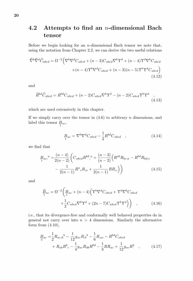
4.2 Attempts to find an n-dimensional Bachtensor
Before we begin looking for an n-dimensional Bach tensor we note that,using the notation from Chapter 2.2, we can derive the two useful relations
∇b∇dCabcd = Ω−2(∇b∇dCabcd + (n− 3)Cabcd∇bΥd + (n− 4)Υd∇bCabcd
+(n− 4)Υb∇dCabcd + (n− 3)(n− 5)ΥbΥdCabcd
)
(4.12)
and
RbdCabcd = RbdCabcd + (n− 2)Cabcd∇bΥd − (n− 2)CabcdΥbΥd ,(4.13)
which are used extensively in this chapter.
If we simply carry over the tensor in (4.6) to arbitrary n dimensions, andlabel this tensor B
1ac,
B1
ac = ∇b∇dCabcd − 12RbdCabcd , (4.14)
we find that
B1
ac;a =
(n− 4)2(n− 2)
(CabcdR
bd;a +
(n− 3)(n− 2)
(RabRbc;a −RbdRbd;c
− 12(n− 1)
RacR;a +
12(n− 1)
RR;c
))(4.15)
and
B1
ac = Ω−2
(B1
ac + (n− 4)(Υb∇dCabcd + Υd∇bCabcd
+12Cabcd∇bΥd + (2n− 7)CabcdΥbΥd
)), (4.16)
i.e., that its divergence-free and conformally well behaved properties do ingeneral not carry over into n > 4 dimensions. Similarly the alternativeform from (4.10),
B2
ac =12Rac;b
b − 112
gacR;bb − 1
6R;ac −RbdCabcd
+ RabRbc − 1
4gacRdbR
bd − 13RRac +
112
gacR2 , (4.17)
August 20, 2004 (15:33)

21
also fails to have these properties in general in n > 4 dimensions since
B2
ac;a =
(n− 4)(n− 2)
(RabRbc;a −RbdRbd;c − (n + 1)
6(n− 1)Ra
cR;a +1
2(n− 1)RR;c
)
(4.18)and
B2
bc =Ω−2B2
bc + (n− 4)Ω−2
(− (n− 2)
2Υa∇dCabcd− (n− 2)
2Υd∇aCabcd
− (n− 3)(n− 2)2
CabcdΥaΥd +(3n− 10)
6ΘRbc
+(n− 3)
2
(gbcRadΘad −ΘabR
ac −RabΘa
c
)+
(8n− 15)6(n− 1)
RΥbΥc
− (3n− 5)4(n− 1)
(Υb∇cR + Υc∇bR
)− (n− 7)(3n− 5)
12(n− 1)gbcΥa∇aR
+(3n2 − 10n + 5)
6(n− 1)RΘbc +
(3n− 5)(n− 7)12(n− 1)
gbcRΥaΥa
− (n− 3)(n− 2)2
(ΘabΘa
c − 12gbcΘadΘad
)− (3n− 10n)
6gbcRΘ
+(3n2 − 16n + 19)
3ΘΘbc− (3n− 5)
2
(Υc∇bΘ + Υb∇cΘ− 1
3∇b∇cΘ
)
− (3n− 5)6
gbc∇a∇aΘ +(n− 7)(3n− 5)
6gbc
(ΘΥaΥa −Υa∇aΘ
)
+ (3n− 5)ΘΥbΥc − (6n2 − 41n + 53)12
gbcΘ2
)(4.19)
where Θab = ∇aΥb−ΥaΥb+ 12gabΥcΥc and Θ = Θa
a = ∇aΥa+ (n−2)2 ΥaΥa.
Going back to the origins of the Bach tensor as an integrability conditionfor conformal Einstein spaces (3.14),
∇b∇dCabcd − (n− 3)(n− 2)
RbdCabcd − (n− 3)(n− 4)ΥbΥdCabcd = 0 (4.20)
suggests considering the tensor
B3
ac = ∇b∇dCabcd − (n− 3)(n− 2)
RbdCabcd
= B1
ac − (n− 4)2(n− 2)
RbdCabcd . (4.21)
But once again, for dimensions n > 4, we see that
B3
ac;a =
(n− 4)(n− 3)(n− 2)2
(RabRbc;a −RbdRbd;c
− 12(n− 1)
RacR;a +
12(n− 1)
RR;c
)(4.22)
August 20, 2004 (15:33)
22
and
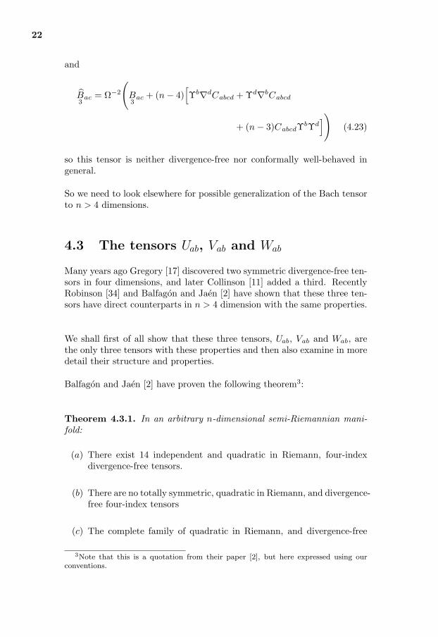
B3
ac = Ω−2
(B3
ac + (n− 4)[Υb∇dCabcd + Υd∇bCabcd
+ (n− 3)CabcdΥbΥd])
(4.23)
so this tensor is neither divergence-free nor conformally well-behaved ingeneral.
So we need to look elsewhere for possible generalization of the Bach tensorto n > 4 dimensions.
4.3 The tensors Uab, Vab and Wab
Many years ago Gregory [17] discovered two symmetric divergence-free ten-sors in four dimensions, and later Collinson [11] added a third. RecentlyRobinson [34] and Balfagon and Jaen [2] have shown that these three ten-sors have direct counterparts in n > 4 dimension with the same properties.
We shall first of all show that these three tensors, Uab, Vab and Wab, arethe only three tensors with these properties and then also examine in moredetail their structure and properties.
Balfagon and Jaen [2] have proven the following theorem3:
Theorem 4.3.1. In an arbitrary n-dimensional semi-Riemannian mani-fold:
(a) There exist 14 independent and quadratic in Riemann, four-indexdivergence-free tensors.
(b) There are no totally symmetric, quadratic in Riemann, and divergence-free four-index tensors
(c) The complete family of quadratic in Riemann, and divergence-free
3Note that this is a quotation from their paper [2], but here expressed using ourconventions.
August 20, 2004 (15:33)
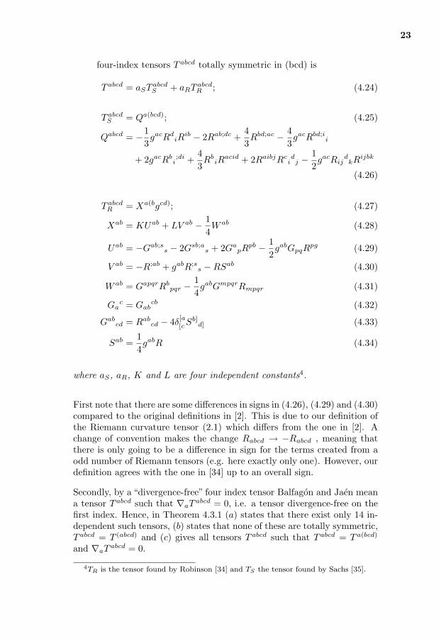
23
four-index tensors T abcd totally symmetric in (bcd) is
T abcd = aST abcdS + aRT abcd
R ; (4.24)
T abcdS = Qa(bcd); (4.25)
Qabcd = −13gacRd
iRib − 2Rab;dc +
43Rbd;ac − 4
3gacRbd;i
i
+ 2gacRbi;di +
43Rb
iRacid + 2RaibjRc
id
j − 12gacRij
dkRijbk
(4.26)
T abcdR = Xa(bgcd); (4.27)
Xab = KUab + LV ab − 14W ab (4.28)
Uab = −Gab;ss − 2Gsb;a
s + 2GapR
pb − 12gabGpqR
pg (4.29)
V ab = −R;ab + gabR;ss −RSab (4.30)
W ab = GapqrRbpqr − 1
4gabGmpqrRmpqr (4.31)
Gac = Gab
cb (4.32)
Gabcd = Rab
cd − 4δ[a[c Sb]
d] (4.33)
Sab =14gabR (4.34)
where aS, aR, K and L are four independent constants4.
First note that there are some differences in signs in (4.26), (4.29) and (4.30)compared to the original definitions in [2]. This is due to our definition ofthe Riemann curvature tensor (2.1) which differs from the one in [2]. Achange of convention makes the change Rabcd → −Rabcd , meaning thatthere is only going to be a difference in sign for the terms created from aodd number of Riemann tensors (e.g. here exactly only one). However, ourdefinition agrees with the one in [34] up to an overall sign.
Secondly, by a “divergence-free” four index tensor Balfagon and Jaen meana tensor T abcd such that ∇aT abcd = 0, i.e. a tensor divergence-free on thefirst index. Hence, in Theorem 4.3.1 (a) states that there exist only 14 in-dependent such tensors, (b) states that none of these are totally symmetric,T abcd = T (abcd) and (c) gives all tensors T abcd such that T abcd = T a(bcd)
and ∇aT abcd = 0.
4TR is the tensor found by Robinson [34] and TS the tensor found by Sachs [35].
August 20, 2004 (15:33)

24
Note that Theorem 4.3.1 implies that the tensors Uab, V ab and W ab areall divergence-free. This follows from the divergence-free property and theconstruction of the tensor T abcd
R via (4.27) and (4.28).
We are specially interested in the tensors Uab, V ab and W ab, and to seetheir inner structure and their properties we write them out in terms of theRiemann curvature tensor, the Ricci tensor and the Ricci scalar,
Ubc =2(n− 3)RabcdRad − (n− 3)Rbc;a
a +(n− 3)
2gbcRadR
ad
+ (n− 3)RRcb +(n− 3)
2gbcR;a
a − (n− 3)4
gbcR2 , (4.35)
Vbc = −R;bc + gbcR;aa −RRbc +
14gbcR
2 , (4.36)
W bc =RbadeRcade − 1
4gbcR
fadeRfade + 2RadRabcd + RRbc
− 2RabRa
c + gbcRadRad − 1
4gbcRR . (4.37)
When we later study the conformal behavior of Uab, V ab and W ab it isuseful to have them expressed in terms of the Weyl tensor, the Ricci tensorand the Ricci scalar,
U bc =2(n− 3)RadCabcd + (n− 3)Rbc;aa − (n− 3)
2gbcR;a
a
+(n− 6)(n− 3)
2(n− 2)gbcRdeR
de +4(n− 3)(n− 2)
RabRa
c
+(n− 3)(n2 − 5n + 2)
(n− 1)(n− 2)RRbc − (n− 3)(n2 − 3n− 6)
4(n− 1)(n− 2)gbcR
2 ,
(4.38)
V bc = −R;bc + gbcR;dd −RRbc +
14gbcR
2 , (4.39)
Wbc = CbadeCcade − 1
4gbcC
fadeCfade +2(n− 4)(n− 2)
CabcdRad
−2(n− 3)(n− 4)(n− 2)2
RabRa
c +(n− 3)(n− 4)
(n− 2)2gbcRadR
ad
+n(n− 3)(n− 4)(n− 1)(n− 2)2
RRbc − (n + 2)(n− 3)(n− 4)4(n− 1)(n− 2)2
gbcR2 . (4.40)
From (4.35) - (4.37) (or (4.38) - (4.40) ) it is obvious that Uab, V ab andW ab are symmetric and quadratic in the Riemann curvature tensor in all
August 20, 2004 (15:33)

25
dimensions. We note from (4.40) that W bc = 0 in four dimensions becausein four dimensions Cb
adeCcade − 14gbcC
fadeCfade = 0, see Appendix B.This fact was not noticed by Collinson [11] but was subsequently pointedout in [34] and [2].
By taking the trace of (4.38) - (4.40) we have
Uaa =− (n− 3)(n− 2)
2R;a
a +(n− 4)(n− 3)
2RadR
ad
− (n− 4)(n− 3)4
R2 , (4.41)
V aa = (n− 1)R;a
a +(n− 4)
4R2 , (4.42)
W aa =− (n− 4)
4CfadeCfade +
(n− 3)(n− 4)(n− 2)
RadRad
− n(n− 3)(n− 4)4(n− 1)(n− 2)
R2 . (4.43)
A simple direct calculation would confirm that Uab, V ab and W ab are alldivergence-free, but we have already noted that this can be deduced fromTheorem 4.3.1.
It is easily checked that the three tensors Uab, V ab and W ab are independentand an obvious question is whether there are any more such tensors; weshall now show that there are not.
Given any symmetric and divergence-free tensor, Y ab, quadratic in theRiemann curvature tensor we see that the tensor Y a(bgcd) is a four-indextensor which is totally symmetric over (bcd), quadratic in the Riemanncurvature tensor and divergence-free (on the first index). Hence we knowfrom Theorem 4.3.1 (c), that there exist constants aS , and aR such that
Y a(bgcd) = aST abcdS + aRT abcd
R (4.44)
holds. Taking the trace over c and d of (4.44) using the facts that
gcdTabcdR = gcdX
a(bcd) = gcd
(KUa(b + LV a(b +
14W a(b
)gcd)
= (n + 2)(KUab + LV ab +
14W ab
), (4.45)
where K and L are constants fixed by (4.44), and
gcdTabcdS =gcdQ
a(bcd) = −43Ra
cRbc +
89R;
ab − 149
Rab;cc
− 19gabR;d
d +169
RcdRadbc +
53RadefRb
def
− 19gabRcdR
cd − 16gabRcdefRcdef , (4.46)
August 20, 2004 (15:33)
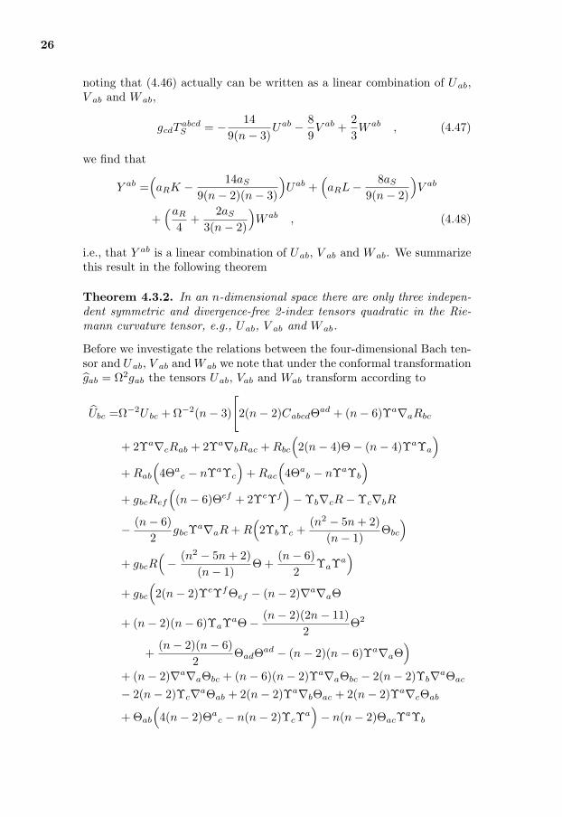
26
noting that (4.46) actually can be written as a linear combination of Uab,V ab and W ab,
gcdTabcdS = − 14
9(n− 3)Uab − 8
9V ab +
23W ab , (4.47)
we find that
Y ab =(aRK − 14aS
9(n− 2)(n− 3)
)Uab +
(aRL− 8aS
9(n− 2)
)V ab
+(aR
4+
2aS
3(n− 2)
)W ab , (4.48)
i.e., that Y ab is a linear combination of Uab, V ab and W ab. We summarizethis result in the following theorem
Theorem 4.3.2. In an n-dimensional space there are only three indepen-dent symmetric and divergence-free 2-index tensors quadratic in the Rie-mann curvature tensor, e.g., Uab, V ab and W ab.
Before we investigate the relations between the four-dimensional Bach ten-sor and Uab, V ab and W ab we note that under the conformal transformationgab = Ω2gab the tensors Uab, Vab and Wab transform according to
Ubc =Ω−2U bc + Ω−2(n− 3)
[2(n− 2)CabcdΘad + (n− 6)Υa∇aRbc
+ 2Υa∇cRab + 2Υa∇bRac + Rbc
(2(n− 4)Θ− (n− 4)ΥaΥa
)
+ Rab
(4Θa
c − nΥaΥc
)+ Rac
(4Θa
b − nΥaΥb
)
+ gbcRef
((n− 6)Θef + 2ΥeΥf
)−Υb∇cR−Υc∇bR
− (n− 6)2
gbcΥa∇aR + R(2ΥbΥc +
(n2 − 5n + 2)(n− 1)
Θbc
)
+ gbcR(− (n2 − 5n + 2)
(n− 1)Θ +
(n− 6)2
ΥaΥa)
+ gbc
(2(n− 2)ΥeΥfΘef − (n− 2)∇a∇aΘ
+ (n− 2)(n− 6)ΥaΥaΘ− (n− 2)(2n− 11)2
Θ2
+(n− 2)(n− 6)
2ΘadΘad − (n− 2)(n− 6)Υa∇aΘ
)
+ (n− 2)∇a∇aΘbc + (n− 6)(n− 2)Υa∇aΘbc − 2(n− 2)Υb∇aΘac
− 2(n− 2)Υc∇aΘab + 2(n− 2)Υa∇bΘac + 2(n− 2)Υa∇cΘab
+ Θab
(4(n− 2)Θa
c − n(n− 2)ΥcΥa)− n(n− 2)ΘacΥaΥb
August 20, 2004 (15:33)

27
+ Θbc
(2(n− 2)(n− 4)Θ− (n− 2)(n− 4)ΥaΥa
)
+ 2(n− 2)ΘΥbΥc
], (4.49)
V bc =Ω−2V bc + Ω−2[− 2(n− 1)ΘRbc − 6RΥcΥb − (n− 4)RΘbc
− (n− 7)gbcRΥaΥa + (n− 4)gbcRΘ + 3Υc∇bR + 3Υb∇cR
+ (n− 7)gbcΥa∇aR− 2(n− 1)∇b∇cΘ + 2(n− 1)gbc∇a∇aΘ+ 6(n− 1)Υc∇bΘ + 6(n− 1)Υb∇cΘ + 2(n− 1)(n− 7)gbcΥa∇aΘ
+ (n− 1)(n− 7)gbcΘ2 − 2(n− 1)(n− 7)ΘgbcΥaΥa
− 12(n− 1)ΘΥbΥc − 2(n− 1)(n− 4)ΘΘbc
], (4.50)
W bc =Ω−2W bc + Ω−2(n− 4)[2CabcdΘad − 2(n− 3)
(n− 2)RabΘa
c
− 2(n− 3)(n− 2)
RacΘab − 2(n− 3)ΘabΘa
c
+2(n− 3)(n− 2)
gbcΘadRad + (n− 3)gbcΘadΘad
+n(n− 3)
(n− 1)(n− 2)RΘbc +
2(n− 3)(n− 2)
RbcΘ
+ 2(n− 3)ΘbcΘ− (n− 3)gbcΘ2
− n(n− 3)(n− 1)(n− 2)
gbcRΘ]
, (4.51)
where Θab = ∇aΥb−ΥaΥb+ 12gabΥcΥc and Θ = Θa
a = ∇aΥa+ (n−2)2 ΥaΥa.
It is easily seen from (4.49) - (4.51) that U bc and V bc are not conformallywell-behaved in general in four dimensions (where W bc = 0).
4.4 Four-dimensional Bach tensor expressedin Uab, Vab and Wab
Since Uab, V ab and W ab constitute a basis for all 2-index symmetric diver-gence-free tensors quadratic in the Riemann curvature tensor, and the Bachtensor Bab has these properties, we must be able to express the Bach tensor(4.6) in four dimensions in terms of Uab and Vab, remembering Wab = 0 infour dimensions.
August 20, 2004 (15:33)

28
In four dimensions we know from (4.38) - (4.39)
U bc =Rbc;aa − 1
2gbcR;a
a + 2CabcdRad + 2RabRc
a
− 12gbcRadR
ad − 13RRbc +
112
gbcR2 (4.52)
V bc = −R;bc + gbcR;aa −RRbc +
14gbcRR (4.53)
Comparing these equations with (4.10) we conclude that we have the rela-tion
Bbc =12U bc +
16V bc . (4.54)
The numerical relationship between the tensors V bc and U bc could also befound using the trace-free property of the Bach tensor. Making the ansatz
Bbc = αU bc + βV bc (4.55)
we see from (4.41) and (4.42) in four dimensions that
Bbb = −αR;b
b + 3βR;bb = −(α− 3β)R;b
b = 0 (4.56)
and hence in general we must have 3α = β.
This link between the Bach tensor Bab and Uab and V ab in four dimensionsdoes not seem to have been noted before.
4.5 An n-dimensional tensor expressed in Uab,Vab and Wab
If we consider the tensor
Bbc =12U bc +
16V bc (4.57)
in n > 4 dimensions, it is clearly divergence-free due to the properties ofUab and V ab, but when we examine its conformal properties we find, aftera lot of work and rearranging,
12Ubc +
16Vbc = Ω−2
(12U bc +
16V bc
)
+ (n− 4)Ω−2[− 1
2(n− 2)(n− 3)CabcdΥaΥd
+ 2(n− 3)Υa∇aRbc − (n− 3)2
Υa∇cRab − (n− 3)2
Υa∇bRac
− (n− 3)2
RabΘac − (n− 3)
2RacΘa
b +(n− 3)
2gbcRadΘad
August 20, 2004 (15:33)
29
+(3n− 7)
3RbcΘ− 1
2Υb∇cR− 1
2Υc∇bR− (3n− 17)
12gbcΥa∇aR
− (3n− 10)6
gbcRΘ +(n− 7)3(n− 5)
2(n− 1)RΥbΥc
+(n− 7)(3n− 5)
12(n− 1)gbcRΥaΥa +
(n− 2)(n− 3)4
gbcΘadΘad
− (n− 2)(n− 3)2
(n− 2)ΘabΘac +
(3n2 − 16 + 19)3
ΘΘbc
+(3n− 5)
2∇b∇cΘ− (3n− 5)
2gbc∇a∇aΘ− 3
(3n− 5)2
Υb∇cΘ
− 3(3n− 5)
2Υc∇bΘ− (n− 7)
(3n− 5)6
gbcΥa∇aΘ
+ 2(3n− 5)
2ΘΥbΥc + (n− 7)
(3n− 5)6
gbcΘΥaΥa
− (6n2 − 41n + 53)12
gbcΘ2]
, (4.58)
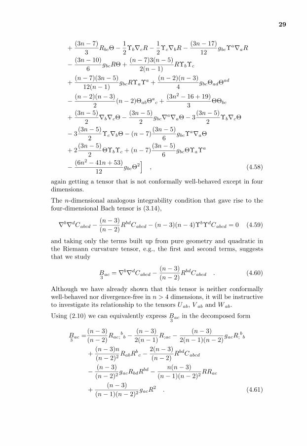
again getting a tensor that is not conformally well-behaved except in fourdimensions.
The n-dimensional analogous integrability condition that gave rise to thefour-dimensional Bach tensor is (3.14),
∇b∇dCabcd − (n− 3)(n− 2)
RbdCabcd − (n− 3)(n− 4)ΥbΥdCabcd = 0 (4.59)
and taking only the terms built up from pure geometry and quadratic inthe Riemann curvature tensor, e.g., the first and second terms, suggeststhat we study
B3
ac = ∇b∇dCabcd − (n− 3)(n− 2)
RbdCabcd . (4.60)
Although we have already shown that this tensor is neither conformallywell-behaved nor divergence-free in n > 4 dimensions, it will be instructiveto investigate its relationship to the tensors Uab, V ab and W ab.
Using (2.10) we can equivalently express B3
ac in the decomposed form
B3
ac =(n− 3)(n− 2)
Rac;bb − (n− 3)
2(n− 1)R;ac − (n− 3)
2(n− 1)(n− 2)gacR;
bb
+(n− 3)n(n− 2)2
RabRbc − 2(n− 3)
(n− 2)RbdCabcd
− (n− 3)(n− 2)2
gacRbdRbd − n(n− 3)
(n− 1)(n− 2)2RRac
+(n− 3)
(n− 1)(n− 2)2gacR
2 . (4.61)
August 20, 2004 (15:33)
30
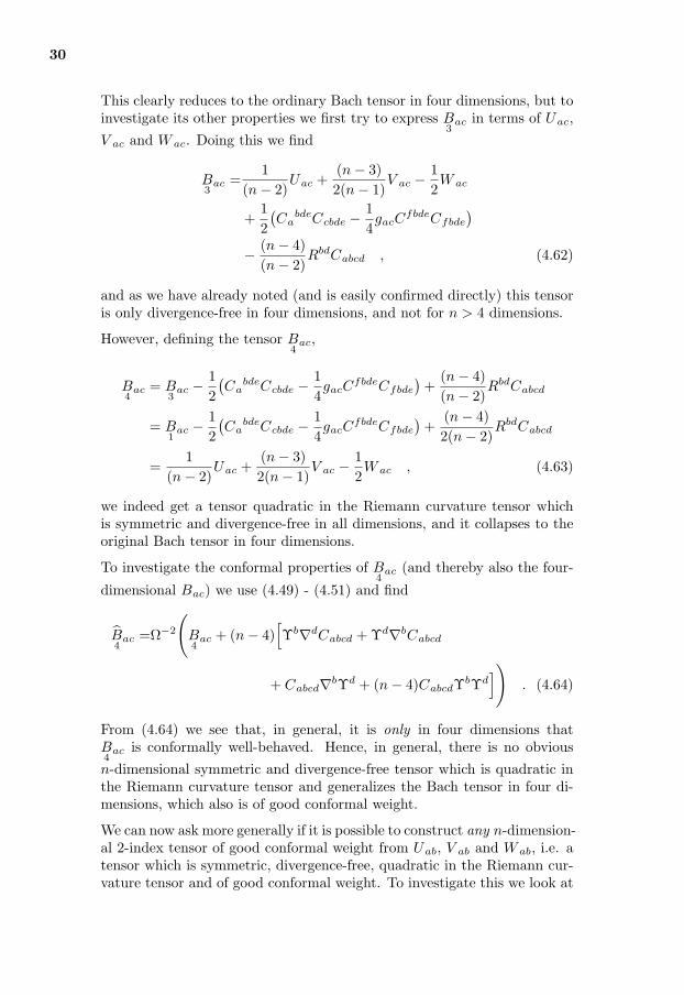
This clearly reduces to the ordinary Bach tensor in four dimensions, but toinvestigate its other properties we first try to express B
3ac in terms of Uac,
V ac and W ac. Doing this we find
B3
ac =1
(n− 2)Uac +
(n− 3)2(n− 1)
V ac − 12W ac
+12(Ca
bdeCcbde − 14gacC
fbdeCfbde
)
− (n− 4)(n− 2)
RbdCabcd , (4.62)
and as we have already noted (and is easily confirmed directly) this tensoris only divergence-free in four dimensions, and not for n > 4 dimensions.
However, defining the tensor B4
ac,
B4
ac = B3
ac − 12(Ca
bdeCcbde − 14gacC
fbdeCfbde
)+
(n− 4)(n− 2)
RbdCabcd
= B1
ac − 12(Ca
bdeCcbde − 14gacC
fbdeCfbde
)+
(n− 4)2(n− 2)
RbdCabcd
=1
(n− 2)Uac +
(n− 3)2(n− 1)
V ac − 12W ac , (4.63)
we indeed get a tensor quadratic in the Riemann curvature tensor whichis symmetric and divergence-free in all dimensions, and it collapses to theoriginal Bach tensor in four dimensions.
To investigate the conformal properties of B4
ac (and thereby also the four-
dimensional Bac) we use (4.49) - (4.51) and find
B4
ac =Ω−2
(B4
ac + (n− 4)[Υb∇dCabcd + Υd∇bCabcd
+ Cabcd∇bΥd + (n− 4)CabcdΥbΥd])
. (4.64)
From (4.64) we see that, in general, it is only in four dimensions thatB4
ac is conformally well-behaved. Hence, in general, there is no obviousn-dimensional symmetric and divergence-free tensor which is quadratic inthe Riemann curvature tensor and generalizes the Bach tensor in four di-mensions, which also is of good conformal weight.
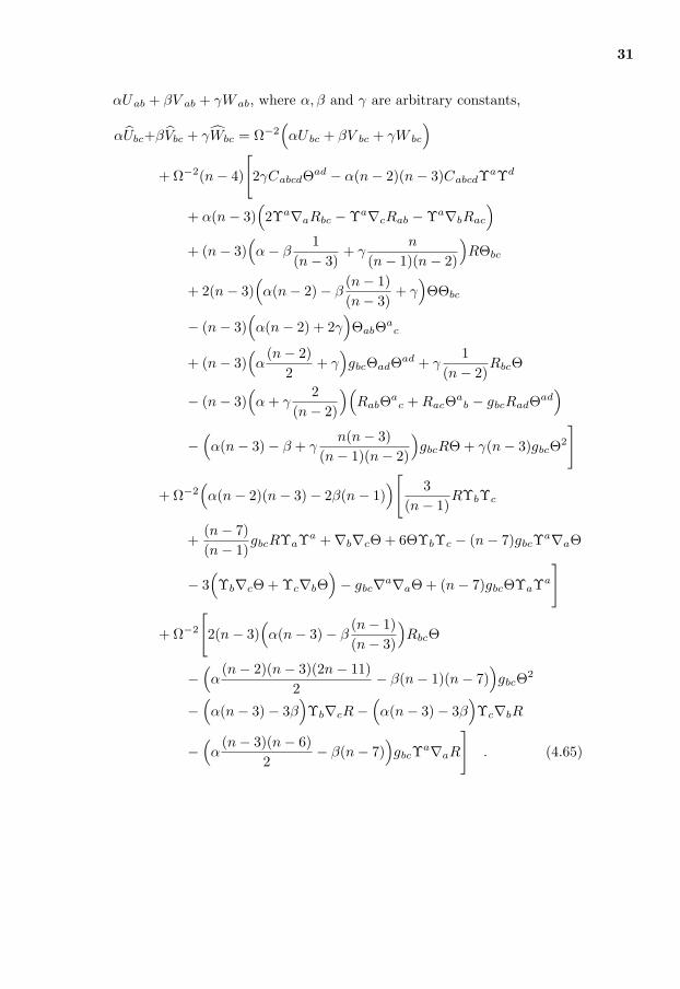
We can now ask more generally if it is possible to construct any n-dimension-al 2-index tensor of good conformal weight from Uab, V ab and W ab, i.e. atensor which is symmetric, divergence-free, quadratic in the Riemann cur-vature tensor and of good conformal weight. To investigate this we look at
August 20, 2004 (15:33)
31
αUab + βV ab + γW ab, where α, β and γ are arbitrary constants,
αUbc+βVbc + γWbc = Ω−2(αU bc + βV bc + γW bc
)
+ Ω−2(n− 4)
[2γCabcdΘad − α(n− 2)(n− 3)CabcdΥaΥd
+ α(n− 3)(2Υa∇aRbc −Υa∇cRab −Υa∇bRac
)
+ (n− 3)(α− β
1(n− 3)
+ γn
(n− 1)(n− 2)
)RΘbc
+ 2(n− 3)(α(n− 2)− β
(n− 1)(n− 3)
+ γ)ΘΘbc
− (n− 3)(α(n− 2) + 2γ
)ΘabΘa
c
+ (n− 3)(α
(n− 2)2
+ γ)gbcΘadΘad + γ
1(n− 2)
RbcΘ
− (n− 3)(α + γ
2(n− 2)
)(RabΘa
c + RacΘab − gbcRadΘad
)
−(α(n− 3)− β + γ
n(n− 3)(n− 1)(n− 2)
)gbcRΘ + γ(n− 3)gbcΘ2
]
+ Ω−2(α(n− 2)(n− 3)− 2β(n− 1)
)[3
(n− 1)RΥbΥc
+(n− 7)(n− 1)
gbcRΥaΥa +∇b∇cΘ + 6ΘΥbΥc − (n− 7)gbcΥa∇aΘ
− 3(Υb∇cΘ + Υc∇bΘ
)− gbc∇a∇aΘ + (n− 7)gbcΘΥaΥa
]
+ Ω−2
[2(n− 3)
(α(n− 3)− β
(n− 1)(n− 3)
)RbcΘ
−(α
(n− 2)(n− 3)(2n− 11)2
− β(n− 1)(n− 7))gbcΘ2
−(α(n− 3)− 3β
)Υb∇cR−
(α(n− 3)− 3β
)Υc∇bR
−(α
(n− 3)(n− 6)2
− β(n− 7))gbcΥa∇aR
]. (4.65)
August 20, 2004 (15:33)
32
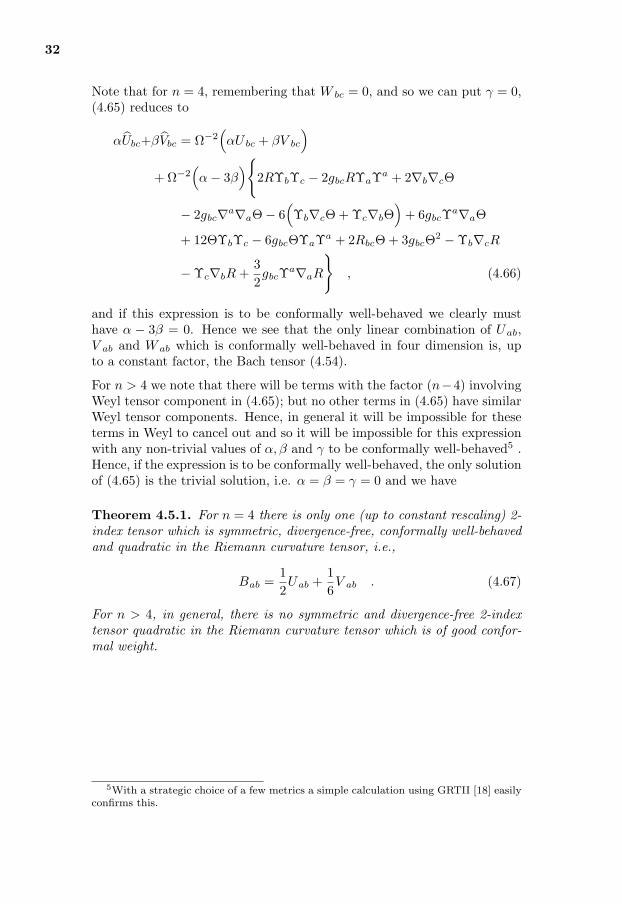
Note that for n = 4, remembering that W bc = 0, and so we can put γ = 0,(4.65) reduces to
αUbc+βVbc = Ω−2(αU bc + βV bc
)
+ Ω−2(α− 3β
)2RΥbΥc − 2gbcRΥaΥa + 2∇b∇cΘ
− 2gbc∇a∇aΘ− 6(Υb∇cΘ + Υc∇bΘ
)+ 6gbcΥa∇aΘ
+ 12ΘΥbΥc − 6gbcΘΥaΥa + 2RbcΘ + 3gbcΘ2 −Υb∇cR
−Υc∇bR +32gbcΥa∇aR
, (4.66)
and if this expression is to be conformally well-behaved we clearly musthave α − 3β = 0. Hence we see that the only linear combination of Uab,V ab and W ab which is conformally well-behaved in four dimension is, upto a constant factor, the Bach tensor (4.54).
For n > 4 we note that there will be terms with the factor (n−4) involvingWeyl tensor component in (4.65); but no other terms in (4.65) have similarWeyl tensor components. Hence, in general it will be impossible for theseterms in Weyl to cancel out and so it will be impossible for this expressionwith any non-trivial values of α, β and γ to be conformally well-behaved5 .Hence, if the expression is to be conformally well-behaved, the only solutionof (4.65) is the trivial solution, i.e. α = β = γ = 0 and we have
Theorem 4.5.1. For n = 4 there is only one (up to constant rescaling) 2-index tensor which is symmetric, divergence-free, conformally well-behavedand quadratic in the Riemann curvature tensor, i.e.,
Bab =12Uab +
16V ab . (4.67)
For n > 4, in general, there is no symmetric and divergence-free 2-indextensor quadratic in the Riemann curvature tensor which is of good confor-mal weight.
5With a strategic choice of a few metrics a simple calculation using GRTII [18] easilyconfirms this.
August 20, 2004 (15:33)

Chapter 5
TheKozameh-Newman-Todfour-dimensional resultand the Bach tensor
Szekeres [39] used spinor methods to attack the problem of finding necessaryand sufficient conditions for a space being conformally Einstein. Indeed hefound a set of conditions written in spinor language, but the equations aredifficult to analyze and rather complicated when translated into tensors1.
However, in 1985 Kozameh, Newman and Tod [27] found a much simplerand more useful set of conditions for spaces for which the complex scalarinvariant
J = ΨABCDΨCDEF ΨEFAB
=18
(Cab
cdCcdefCef
ab − i∗Cabcd∗Ccd
ef ∗Cefab
)(5.1)
of the Weyl spinor/tensor is nonzero. Their set involves the Bach tensorintroduced in the previous chapters.
In this chapter we will use a tensor/spinor approach to review both the ex-plicit and the implicit four-dimensional results of KNT2 [27]. Since spinorsare used in this chapter we are restricted to four-dimensional spaces withsignature (+ − −−). To some extent the presentation here follows theoriginal paper by KNT [27], although some of our proofs are more direct.
1In fact there is a small mistake in [39] pointed out by Wunsch [43] making some ofthe results in [39] incorrect and the conditions only necessary.
2Kozameh, Newman and Tod.
August 20, 2004 (15:33)
34
5.1 Two useful lemmas
In the proof of the KNT result the following two lemmas play a key role:
Lemma 5.1.1. Given a skew-symmetric real tensor F ab = F [ab], then,provided J 6= 0, the only solution of the equation
CabcdFcd = 0 (5.2)
is F cd = 0.
Lemma 5.1.2. Given a symmetric and trace-free real tensor Hab = H(ab),then, provided J 6= 0, the only solution of
CabcdHad = 0 (5.3)
and∗CabcdH
ad = 0 (5.4)
is Had = 0.
The proof of these two lemmas can be given simultaneously using spinors:
Proof. A skew-symmetric real tensor F ab = F [ab] can be written in spinorlanguage as
F ab = FAA′BB′ = φABεA′B′ + φA′B′εAB (5.5)
where φAB = φ(AB) is a symmetric spinor. A symmetric real trace-freetensor Hab = H(ab) can be written as
Hab = HAA′BB′ = φABA′B′ (5.6)
where φABA′B′ = φ(AB)(A′B′).
In this notation equation (5.2) and (5.3), (5.4) become
ΨABCDφCD = 0 (5.7)
andΨABCDφCD
A′B′ = 0 (5.8)
respectively, ΨABCD being the Weyl spinor. Hence we see that the primedindices play no role in (5.8) and we only need to consider the equation
ΨABCDφCD = 0 (5.9)
and show that under the assumption that J 6= 0 this implies φCD = 0.Note that we can consider
φAB −→ ΨABCDφCD (5.10)
August 20, 2004 (15:33)
35
as a linear mapping from symmetric 2-index spinors to symmetric 2-indexspinors and hence we can study the properties of the mapping via its matrixrepresentation Ψ (see Appendix A.3). So, we can represent (5.9) by thematrix equation
Ψx = 0 , (5.11)
where x is the vector representation of φAB . If detΨ 6= 0, then the onlysolution of equation (5.11) is the trivial one, x = 0.
From (A.25) we have that
det(Ψ) =13J (5.12)
and hence under the assumption J 6= 0 the only solution to (5.9) is thetrivial solution, i.e. φCD = 0. This completes the proof of both lemmas.
Using tensors the first of these lemmas, Lemma 5.1.1, can easily be provedin an analogous manner as when using spinors. This is because the Weyltensor Cabcd in this case can be looked upon as a linear mapping taking2-forms to 2-forms. Hence, as shown in appendix A, the properties ofthe mapping can be studied using its matrix representation, C, and fromAppendix C we know that
det(C) =19JJ (5.13)
and hence if J 6= 0, then det(C) 6= 0 and the only solution of (5.2) is thetrivial one.
The second lemma, Lemma 5.1.2, is harder to prove just using tensor meth-ods, and is a good example of the power of using spinors when working infour dimensions; the result is almost trivial to prove in spinors, but is muchharder using tensors.
5.2 C-spaces and conformal C-spaces
Szekeres [39] introduced a class of spaces called C-spaces and this class isdefined by
Definition 5.2.1. A space is a C-space if the space has a divergence-freeWeyl tensor3, i.e.,
∇dCabcd = 0 . (5.14)
Since we are interested in conformal spaces we also have the definition
3Sometimes a Weyl tensor satisfying (5.14) is called a harmonic Weyl tensor ; see forinstance [28].
August 20, 2004 (15:33)

36
Definition 5.2.2. A space is a conformal C-space if there exists a confor-mal transformation gab = Ω2gab such that ∇dCabcd = 0.
The condition ∇dCabcd = 0 written out in the space with metric gab is
∇dCabcd + ΥdCabcd = 0 (5.15)
where Υd = ∇d(ln Ω).
On the other hand if
∇dCabcd + KdCabcd = 0 (5.16)
holds for any vector field Ka we see that by taking ∇c of equation (5.16)and then using (5.16) we have
∇c∇dCabcd +∇cKdCabcd −KcKdCabcd = 0 . (5.17)
Using the facts that the last term in this expression (5.17) vanishes andthat (independently of dimension) ∇c∇dCabcd = 0 we find
∇cKdCabcd = ∇[cKd]Cabcd = 0 . (5.18)
Hence from (5.18) and Lemma 5.1.1 we conclude that in a space in whichJ 6= 0 it follows that ∇[cKd] = 0, locally giving us a gradient vector fromwhich the conformal factor can be found. So, we have the first part of theKNT result [27],
Theorem 5.2.1. A space in which J 6= 0 is locally conformal to a C-spaceif and only if there exists a vector field Ka such that
∇dCabcd + KdCabcd = 0 . (5.19)
Furthermore, Ka is unique.
To see that the vector Kd in Theorem 5.2.1 is unique suppose there existsanother vector ξa satisfying (5.19), i.e.,
∇dCabcd + ξdCabcd = 0 . (5.20)
Subtracting (5.20) from (5.19) and setting ηa = Ka − ξa we then have
ηdCabcd = 0 . (5.21)
Multiplying this with an arbitrary vector field ζc,
ζcηdCabcd = ζ [cηd]Cabcd = 0 , (5.22)
August 20, 2004 (15:33)

37
and since J 6= 0 this equation implies that ζ [cηd] = 0 for all vector fields ζa.But this can only be true if ηa = 0, i.e., if Ka = ξa, and hence Theorem5.2.1 is proved4.
We can have alternative versions of Theorem 5.2.1. Consider the four-dimensional identities5,
CibcdCjbcd =14δijC
abcdCabcd , (5.23)
CibcdC
cdefCef
jb =14δijC
abcdC
cdefCef
ab , (5.24)
∗CibcdCjbcd =14δij∗CabcdCabcd , (5.25)
∗Cibcd∗Ccd
ef∗Cef
jb =14δij∗Cab
cd∗Ccd
ef∗Cef
ab . (5.26)
If CabcdCabcd 6= 0, we can multiply (5.19) by Cabce to obtain
Cabce∇dCabcd +14KeCabcdC
abcd = 0 . (5.27)
By dividing (5.27) with C2 = CabcdCabcd we are actually able to express
the vector in pure geometric terms:
Ke = −4Cabce∇dCabcd/C2 . (5.28)
Analogously, we get from (5.24) - (5.26), provided the corresponding scalarinvariant of the Weyl tensor is nonzero,
Ke =− 4∗Cabce∇dCabcd/C∗C , (5.29)
Ke =− 4CabklCklce∇dCabcd/C3 , (5.30)
Ke =− 4∗Cabkl∗Cklce∇dCabcd/
∗C3 . (5.31)
We can now restate Theorem 5.2.1 as
Theorem 5.2.2. A space is conformal to a C-space if
∇dCabcd + KdCabcd = 0 (5.32)
holds with Ka defined by (at least) one of the equations (5.28) - (5.31).
We comment on the case when J = 0 in the last section of this chapter.
4There is another way to prove the uniqueness of Ka using J 6= 0 to solve for Ka
explicitly, and this is illustrated in Chapter 8.5See appendix B for their derivation.
August 20, 2004 (15:33)

38
5.3 Conformal Einstein spaces
We know from Chapter 3 that a four-dimensional space is conformallyEinstein if and only if there exists a conformal transformation gab = Ω2gab
such that
Rab − 14gabR− 2∇aΥb +
12gab∇cΥc − 2ΥaΥb +
12gabΥcΥc = 0 (5.33)
where Υa = ∇a(lnΩ).
The first integrability condition of (5.33) is, as calculated in (3.12),
∇dCabcd + ΥdCabcd = 0 , (5.34)
meaning that conformal Einstein spaces constitute a subclass of conformalC-spaces, and that being a conformal C-space is a necessary condition fora space to be conformally Einstein;
Theorem 5.3.1. A conformal Einstein space is also conformal to a C-space.
On the other hand, in four dimensions we found another necessary conditionfor a space being conformally Einstein in (3.15), the vanishing of the Bachtensor,
Bbc = ∇a∇dCabcd − 12RadCabcd = 0 , (5.35)
and in fact (5.34) together with (5.35) are also sufficient provided J 6= 0.
To prove this we will use Lemma 5.1.2. First observe that if J 6= 0 thenby the same argument as was used to prove Theorem 5.2.1 it follows thatequation (5.34) is satisfied with Υa = ∇a(ln Ω) for some scalar field Ω.Hence, differentiating (5.34),
∇a∇dCabcd +(∇aΥd −ΥaΥd
)Cabcd = 0 (5.36)
and subtracting (5.35) we have
Cabcd
(Rad + 2∇aΥd − 2ΥaΥd
)= 0 . (5.37)
This equation (5.37) will serve as the first equation in Lemma 5.1.2 withHad = Rad + 2∇aΥd − 2ΥaΥd.
To obtain the second equation in Lemma 5.1.2 we first take the dual ofequation (5.34),
∇d∗Cabcd + Υd∗Cabcd = 0 (5.38)
and then differentiate this with ∇a to find
∇a∇d∗Cabcd +(∇aΥd −ΥaΥd
)∗Cabcd = 0 . (5.39)
August 20, 2004 (15:33)

39
By taking the divergence of the dual of the contracted Bianchi identity(2.8),
0 = ∇b∇d∗Cabc
d + ηabpq
(∇b∇[pRq]c −
13gc[q∇b∇p]R
), (5.40)
and using the Ricci identity and (2.5) to decompose the Riemann curvaturetensor into its irreducible parts we get
∇a∇d∗Cabcd − 12Rad∗Cabcd = 0 . (5.41)
Hence subtracting (5.41) from (5.39) gives
∗Cabcd
(Rad + 2∇aΥd − 2ΥaΥd
)= 0 , (5.42)
i.e., the second equation in Lemma 5.1.2.
Equations (5.37) and (5.42) applied to Lemma 5.1.2 now give us that
Rad + 2∇aΥd − 2ΥaΥd =14gadT , (5.43)
with T being the trace of the left hand side of (5.43). Hence (5.43) isequivalent to
Rab − 14gabR + 2∇aΥb +
12gab∇cΥc − 2ΥaΥb +
12gabΥcΥc = 0 . (5.44)
Since we know Υa = ∇a(lnΩ) it follows from Section 3.2 that the space isa conformal Einstein space, and so we have proven the main result in KNT[27],
Theorem 5.3.2. A space in which J 6= 0 is a conformal Einstein space ifand only if there exists a vector field Ka such that
∇dCabcd + KdCabcd = 0 , (5.45)
Bbc = ∇a∇dCabcd − 12RadCabcd = 0 . (5.46)
Note that this set of conditions naturally divide into two sets; condition(5.45) selects the class of C-spaces, and condition (5.46) specifies a partic-ular subclass of the C-spaces.
The natural question arises if both the conditions (5.45) and (5.46) in The-orem 5.3.2 really are needed, or if one of them is redundant. However, aspointed out in [27], the Newman-Kerr metric (subject to the parameterrestrictions a = 0 and e 6= 0) provides an example of a space where J 6= 0and although it has non-vanishing Bach tensor, Bab 6= 0, it is a conformalC-space. Hence it is not enough that a space is conformal to a C-space to
August 20, 2004 (15:33)
40
be conformally Einstein. Also Kozameh et al. [27] provide an argument,suggested by R. Geroch and G. T. Horowitz, based on counting initial data,showing that the conditions (5.45) and (5.46) are independent, and henceboth needed. But this falls short of providing a specific counterexample tothe possibility of one of (5.45) or (5.46) being redundant.
On the other hand, Nurowski and Plebananski [31] recently found a typeN metric of the Feferman class which has vanishing Bach tensor, Bab = 0,but which is not conformal to an Einstein space6. Hence, in the case of ageneral space, it is not enough that the Bach tensor vanishes for a space tobe conformal to an Einstein space. However, we emphasize that this metrichas7 J = 0 and so is not strictly relevant to our theorem. Therefore thepossibility of a zero Bach tensor together with the condition J 6= 0 beingsufficient for a conformally Einstein space is still open.
The condition (5.46), the vanishing of the Bach tenor, has been discussedin different contexts by a number of authors [25], [27], [30]. Also note thatin an alternative theorem to Theorem 5.3.2 for the existence of conformalEinstein spaces by Baston and Mason [3], [4] for spaces in which I 6= 0 theBach tensor is chosen to be zero, but the condition (5.45) is replaced withanother condition formulated in spinors as a restriction on the Weyl spinor.
5.4 J = 0
When we put the condition J 6= 0 on a space-time we exclude space-timesof Petrov type III, N , and some particular cases of type I. In theseother cases the conditions in Theorem 5.3.2 do not provide necessary andsufficient conditions on a space being conformally Einstein, i.e., it is notenough to demand that the space is a conformal C-space and the vanishingof the Bach tensor.
Later Wunsch [44], also using a spinor approach, derived necessary andsufficient conditions for space-times of type III to be conformally Einstein.The conditions Wunsch found are the two in Theorem 5.3.2 plus an addi-tional one involving the vanishing of a scalar defined by four contractionsbetween a trace-free and symmetric tensor constructed from the geometryand a preferred vector constructed from a special choice of spin basis forspace-times of Petrov type III. That these conditions are not sufficient fora space-time of Petrov type N to be conformally Einstein is provided bythe example of generalized plane wave space-times [43].
The Petrov type N case is still unsolved, but in the pursuit of the solutionCzapor, McLenaghan and Wunsch [12] derived necessary and sufficientconditions for a space-time of Petrov type N to be conformally related
6The spaces in the Feferman class have the property that they are not conformal toa Einstein space.
7This is a property of all type N metrics.
August 20, 2004 (15:33)

41
to an empty space (Rab = 0), as well as some sufficient conditions for aspace-time of Petrov type N to be conformal to a C-space.
August 20, 2004 (15:33)

Chapter 6
Listing’s result in fourdimensions
In this chapter we will describe the recent generalization of the KNT resultin Chapter 5 due to Listing [28]. In his paper he looks at the problem withmore emphasis on the differential geometry point of view, which makessome of his quantities and equations awkward to translate into tensors orspinors. We will restrict ourselves to four-dimensional spaces throughoutthis chapter.
6.1 Non-degenerate Weyl tensor
When we proved the results of KNT the two Lemmas 5.1.1 and 5.1.2 playeda key role and to prove these we had to impose a restriction on the spacesunder consideration. The restriction was found from a spinor point of viewand was J 6= 0.
However, it is well known that locally we can look upon the Weyl tensoras a linear mapping between two-forms, i.e., given F ab = F [ab] then
F ab −→ CabcdF
cd . (6.1)
Thereby it is possible to translate the Weyl tensor into a matrix, C (seeappendix A), and to study properties of the mapping (6.1) using this rep-resentation of the Weyl tensor.
It can be shown, see Appendix C, that in four dimensions the conditionJ 6= 0 is equivalent to the condition det(C) 6= 0, meaning that imposingdet(C) 6= 0 the mapping (6.1) is injective. Hence, given any two-formF ab = F [ab] the only solution of the equation Cab
cdFcd = 0 in a space
where det(C) 6= 0 is F cd = 0, and in such a space, Lemma 5.1.1 of KNT
August 20, 2004 (15:33)
43
holds1.
Definition 6.1.1. If det(C) 6= 0 the Weyl tensor is said to be non-degene-rate.
The fact that the Weyl tensor is non-degenerate means that there is aninverse, i.e., that there exists a tensor field Dab
cd such that
DabcdC
cdef = δa
[eδbf ] , (6.2)
where δa[eδ
bf ] is the “identity” in Λ2. When the Weyl tensor Cab
cd is consid-ered as a matrix C, then the inverse, Dab
cd, is the matrix C−1. In practicethe tensor Dab
cd is not explicitly known and to interpret C−1 in tensornotation cannot easily be done2.
6.2 Conformal C-spaces
In the spaces where det(C) 6= 0 we can use Dabcd to get an alternative
characterization of conformal C-spaces to the one presented in the previouschapter.
From Theorem 5.2.1 we know that a space for which det(C) 6= 0 is confor-mally a C-space if and only if there exist a vector field Ka such that
∇dCabcd + KdCab
cd = 0 . (6.3)
Multiplying (6.3) with Defab and using (6.2) we have
0 = Defab∇dCab
cd + KdDefabC
abcd
= Defab∇dCab
cd + Kdδe[cδ
fd] , (6.4)
and by taking the trace over c and f and solving for the vector field we find
Ke =23Dec
ab∇dCabcd . (6.5)
Hence, using Dabcd we are able to get an expression for the vector field Ka
and we can now formulate the corresponding theorem to Theorem 5.2.2,
Theorem 6.2.1. A space having a non-degenerate Weyl tensor is locallyconformal to a C-space if and only if (6.3) holds with Ka defined by (6.5).
Note that the central difference between Theorem 5.2.2 and Theorem 6.2.1is the expressions defining the vector field Ka.
1Also, since det(C) 6= 0 ⇔ J 6= 0, in fact Lemma 5.1.2 of KNT holds, but how totranslate the Weyl tensor to a matrix and how to interpret it in this case is not clear.
2We will see in Chapter 8 that we can avoid the use of the tensor Dabcd.
August 20, 2004 (15:33)
44
6.3 Conformal Einstein spaces
To prove Theorem 5.3.2 of KNT we needed both the Lemmas 5.1.1 and5.1.2, and indeed, as noted in the previous section, if the Weyl tensor isnon-degenerate both these lemmas hold.
However, in a space with non-degenerate Weyl tensor we can always definethe vector field Ke as done in (6.5), i.e. such that
Ke =23Dec
ab∇dCabcd (6.6)
and this give us the following characterization of the conformal Einsteinspaces:
Theorem 6.3.1. A space with non-degenerate Weyl tensor is locally con-formal to an Einstein space if and only if the vector field Ka defined in(6.6) satisfies
Rab − 14gabR + 2∇aKb +
12gab∇cK
c − 2KaKb +12gabKcK
c = 0 . (6.7)
Proof. If (6.7) holds we see by skewing (6.7) that ∇[aKb] = 0, i.e. thatKa locally is a gradient from which the conformal factor can be found andhence the space is conformally Einstein.
Conversely, if the space is conformally Einstein equation (6.7) is satisfiedfor some (gradient) vector field Ka. Also, from Theorem 5.3.1 we have thatthe space is conformally a C-space, and Theorem 6.2.1 then tells us thatthis vector is unique and hence is the one given by (6.6).
Note the difference between Theorem 5.3.2 and Theorem 6.3.1 though bothhave the same generic setting (det(C) 6= 0 or equivalently J 6= 0 ). Thetwo ingredients in Theorem 5.3.2 are the conditions that the space is aconformal C-space and the vanishing of the Bach tensor: the first conditionis the first integrability condition for a space being conformally Einstein,and the second one arise from taking a derivative of the first one.
In Theorem 6.3.1 on the other hand the condition of being a conformalEinstein space and an explicit expression for the vector field Ka are theconditions. However, in the construction of Ka we use the condition thatthe space is a conformal C-space, and hence Ka “contains” the first inte-grability condition for the space being conformally Einstein.
August 20, 2004 (15:33)

Chapter 7
Listing’s result in ndimensions
In this chapter we briefly comment on the extension of the definition ofthe non-degenerate Weyl tensor to arbitrary n dimensions. We will alsogive the n-dimensional counterparts of Theorem 6.2.1 and Theorem 6.3.1from the previous chapter as well as Theorem 5.2.1 and Theorem 5.3.1 inChapter 5. The theorems are essentially the same as those given by Listing[28] although the formulation and notation differs somewhat.
7.1 Non-degenerate Weyl tensor
The concept of a non-degenerate Weyl tensor introduced in Chapter 6.1transfers directly to arbitrary n dimensions and we define
Definition 7.1.1. An n-dimensional space is said to have a non-degenerateWeyl tensor if the determinant of the matrix C associated with the linearmapping
F ab −→ CabcdF
cd , F cd = F [cd] (7.1)
is non-zero, i.e., if detC 6= 0.
It follows directly that from the definition 7.1.1 that in a space with non-degenerate Weyl tensor the equation
CabcdF
cd = 0 , F cd = F [cd] (7.2)
only has the trivial solution, F cd = 0.
In a space with non-degenerate Weyl tensor there exist a tensor field Dabcd
such thatDab
cdCcd
ef = δa[eδ
bf ] , (7.3)
where δa[eδ
bf ] is the “identity” in the space of two-forms.
August 22, 2004 (16:21)
46
7.2 Conformal C-spaces
Before we formulate and prove the n-dimensional version of Theorem 6.2.1we first note that the four-dimensional Theorem 5.2.1 has a natural exten-sion to n-dimensional spaces with non-degenerate Weyl tensor:
Theorem 7.2.1. An n-dimensional space with non-degenerate Weyl tensoris locally conformal to a C-space if and only if there exists a vector field Ka
such that∇dCab
cd + (n− 3)KdCabcd = 0 . (7.4)
Furthermore, Ka is unique.
Proof. The proof is analogous to the four-dimensional theorem. If the spaceis a conformal C-space there exists a conformal transformation gab = Ω2gab
such that ∇dCabcd = 0 holds, i.e., expressed in the space with metric gab
such that (7.4) holds with Υa = ∇a(lnΩ).
If on the other hand (7.4) holds we see by differentiating (7.4), using∇c∇dCab
cd = 0 and (7.4) again, that
∇cKdCabcd = ∇[cKd]Cab
cd = 0 , (7.5)
i.e., provided the that the Weyl tensor is non-degenerate that ∇[cKd] = 0.Hence Kd is locally a gradient from which the conformal factor can befound.
Clearly a vector field satisfying (7.4) must be unique since in a given spacewith non-degenerate Weyl tensor both Cab
cd and Dabcd are uniquely de-
termined. Hence, using Defab on (7.4), taking a trace over c and f and
solving for Ke we find
Ke =2
(n− 1)(n− 3)Dec
ab∇dCabcd , (7.6)
which clearly must be unique.
As a matter of fact the previous proof also proves the n-dimensional versionof Theorem 6.2.1:
Theorem 7.2.2. An n-dimensional space having a non-degenerate Weyltensor is locally conformal to a C-space if and only if
∇dCabcd + (n− 3)KdCab
cd = 0 (7.7)
holds with the vector field Ka defined by
Ke =2
(n− 1)(n− 3)Dec
ab∇dCabcd . (7.8)
August 20, 2004 (15:33)
47
7.3 Conformal Einstein spaces
We close this chapter with the n-dimensional version of Theorem 6.2.1 andagain the proof is very similar to the four-dimensional one.
First note that an n-dimensional space is conformally Einstein if and onlyif there is a conformal transformation gab = Ω2gab such that
Rab − 1n
gabR + (n− 2)∇aΥb − (n− 2)n
gab∇cΥc
− (n− 2)ΥaΥb +(n− 2)
ngabΥcΥc = 0 , (7.9)
where Υa = ∇a(lnΩ), and that the first integrability condition of (7.9), asfound in (3.12), is
∇dCabcd + (n− 3)ΥdCab
cd = 0 ; (7.10)
hence we have the n-dimensional version of Theorem 5.3.1
Theorem 7.3.1. A conformal Einstein space is conformal to a C-space.
Finally we have Listing’s n-dimensional result,
Theorem 7.3.2. An n-dimensional space with a non-degenerate Weyl ten-sor is locally conformal to an Einstein space if and only if the vector fieldKa defined by
Ke =2
(n− 1)(n− 3)Dec
ab∇dCabcd (7.11)
satisfies
Rab − 1n
gabR + (n− 2)∇aKb − (n− 2)n
gab∇cKc
− (n− 2)KaKb +(n− 2)
ngabKcK
c = 0 . (7.12)
Proof. If (7.12) holds we see by skewing (7.12) that ∇[aKb] = 0, i.e., thatKa is locally a gradient from which the conformal factor can be found andhence the space is conformally Einstein.
Conversely, if the space is conformally Einstein, equation (7.12) is satisfiedfor some (gradient) vector field Υa. Also, from Theorem 7.3.1 we have thatthe space is conformally a C-space, and Theorem 7.2.2 then tells us thatthis vector field is unique and hence is the one given by (7.8).
August 20, 2004 (15:33)

Chapter 8
Edgar’s result in ndimensions
In this chapter we shall show how Edgar [13] reformulated the results ofKNT and Listing and showed how to get an explicit expression for thevector field Ka in Theorems 7.2.2, 7.3.2 without using the inverse map ofListing.
The procedure (essentially using the Cayley-Hamilton Theorem) gives usa generic expression in n dimensions, but due to dimensionally dependentidentities we are able to get expressions of considerable lower order. Ex-amples in 4, 5 and 6 dimensions are discussed in detail.
8.1 Using the Cayley-Hamilton Theorem
We show how we can get around the implicit construction of the vectorfield Ka in the work of Listing. The non-degeneracy condition we imposeon the Weyl tensor, formulated in the matrix representation of the Weyltensor, is det(C) 6= 0, e.i., the same as used by KNT and Listing.
First we prove the following useful lemma:
Lemma 8.1.1. In an n-dimensional space in which det(C) 6= 0 the inho-mogeneous algebraic equation for the vector field ξd
Cabcdξ
d = Habc (8.1)
has the unique solution,
ξa =2
(n− 1)cNHef
b
(c0C[N − 1]ab
ef + c2C[N − 3]abef
+ c3C[N − 4]abef + . . . + cN−2C
abef
), (8.2)
August 20, 2004 (15:33)

49
where N = n(n− 1)/2. The coefficients c0, c1, . . ., cN−2, cN are the usualcharacteristic coefficients of the Cayley-Hamilton Theorem given in (A.6).
Proof. If we consider the Cayley-Hamilton Theorem for the N × N ma-trix C, see Appendix A (A.5), in tensor notation, with the characteristiccoefficients given by (A.6), remembering that c1 = 0 since C is trace-free,
c0C[N ]abcd + c2C[N − 2]ab
cd + c3C[N − 3]abcd + . . .
. . . + cN−2C[2]abcd + cN−1C[1]ab
cd + cNδa[cδ
bd] = 0 , (8.3)
we obtain by multiplying by ξa
ξa
(c0C[N ]ab
cd + c2C[N − 2]abcd + c3C[N − 3]ab
cd + . . .
. . . + cN−2C[2]abcd + cN−1C[1]ab
cd
)+ cNξ[cδ
bd]
=ξaCabef
(c0C[N − 1]ef
cd + c2C[N − 3]efcd + c3C[N − 4]ef
cd + . . .
. . . + cN−2C[1]efcd
)+ cN−1ξaCab
cd + cNξ[cδbd] = 0 . (8.4)
Taking the trace over b and d, remembering that the Weyl tensor is trace-free we find
ξaCabef
(c0C[N − 1]ef
cb + c2C[N − 3]efcb + c3C[N − 4]ef
cb + . . .
. . . + cN−2C[1]efcb
)+
(n− 1)2
cNξc = 0 . (8.5)
Since cN = (−1)N det(C) and det(C) 6= 0 there is no problem dividingwith cN and a trivial rearranging of the terms in this last equation givesthe required expression (8.2).
Using Lemma 8.1.1 on
∇dCabcd + (n− 3)KdCab
cd = 0 , (8.6)
i.e., setting Habc = KdCab
cd = − 1(n−3)∇dCab
cd, we can directly reformu-late Theorem 6.3.1 as
Theorem 8.1.1. A n-dimensional space having a non-degenerate Weyltensor is locally conformal to an Einstein space if and only if the vectorfield Ka defined by
Ka =2
(n− 1)(n− 3)cN∇dCef
db
(c0C[N − 1]ab
ef + c2C[N − 3]abef
+ c3C[N − 4]abef + . . . + cN−2C
abef
), (8.7)
August 20, 2004 (15:33)

50
where N = n(n− 1)/2 satisfies
Rab − 1n
gabR + (n− 2)∇aKb − (n− 2)n
gab∇cKc
− (n− 2)KaKb +(n− 2)
ngabKcK
c = 0 . (8.8)
Note that substituting (8.7) into (8.8) gives necessary and sufficient condi-tions defined in terms only depending on the geometry.
Four dimensions
In four dimensions N = 6, and from (8.7) in Theorem 8.1.1 we get thefollowing expression for the vector field
Ka =2
3c6∇dCef
db
(c0C[5]ab
ef + c2C[3]abef
+ c3C[2]abef + c4C
abef
). (8.9)
It is clear that this expression involves powers of the Weyl tensor up to thesixth order, but since the vector of the theorems is unique there must bea link between the expression (8.9) and the ones given by KNT, (5.28) -(5.31), and Listing, (6.5). This link has been exploited by Edgar [13].
Higher dimensions
Theorem 8.1.1 supplies an explicit expression for the vector field Ka in alldimensions n ≥ 4. For example, in six dimensions where N = 15 we have
Ka =2
15c15∇dCef
db
(c0C[14]ab
ef + c2C[12]abef + c3C[11]ab
ef
+ . . . + c11C[3]abef + c12C[2]ab
ef + c13Cab
ef
), (8.10)
and clearly this expression contains powers of the Weyl tensor up to fif-teenth order.
In general, Theorem 8.1.1 gives an expression of the vector field Ka foran n-dimensional space containing powers of the Weyl tensor up to ordern(n − 1)/2. Hence, the generic expression for Ka quickly grows in size asthe dimension becomes higher and higher.
However, in four dimensions we have seen that the generic expression (8.9),having powers of the Weyl tensor up to sixth order, can be replaced withan expression with much lower powers in the Weyl tensor obtained fromdimensionally dependent identities. In the next section we will extend thisapproach to spaces of arbitrary dimension n.
August 20, 2004 (15:33)
51
8.2 Using dimensionally dependent identities
The method used by KNT to get their vector field1 Ka was to assumethat (at least) one of the scalar invariants of the Weyl tensor is non-zeroand use one of the dimensionally dependent identities (5.23) - (5.26) on theequation
∇dCabcd + KdCabcd = 0 . (8.11)
All four identities (5.23) - (5.26) are, as discussed in appendix B, a conse-quence of the four-dimensional identity
C [ab[cdδ
i]j] = 0 (8.12)
and they arise when we multiply (8.12) with more Weyl tensors.
The structure of these identities are of the type
LC[m]ij =14δijLC[m] (8.13)
where LC[m]ij represents a 2-index tensor consisting of a linear combina-tion of products of m Weyl tensors, and LC[m] ≡ LC[m]ii representsa linear combination of scalar products of m Weyl tensors.
In general, an n-dimensionally dependent identity arising from the n-dimen-sional analogue to (8.12) (see appendix B) has the structure
LC[m]ij =1n
δijLC[m] . (8.14)
Hence, for LC[m] 6= 0, we can use (8.14) on the n-dimensional analogueto (8.11),
∇dCabcd + (n− 3)KdCabcd = 0 (8.15)
to get the following expression for the vector field Ka
Ki = nLC[m]ijKj/LC[m] , (8.16)
where all the terms involving the vector field Ka on the right hand side −which will each contain a factor of the form Cab
cjKj − can be replaced
using (8.15), i.e.,
CabcjK
j = − 1(n− 3)
∇jCabcj . (8.17)
Using the notation introduced above we are now able to state the followingtheorem generalizing Theorem 5.3.2 of KNT,
1The same method was also used by Listing in [28] in his examples.
August 20, 2004 (15:33)
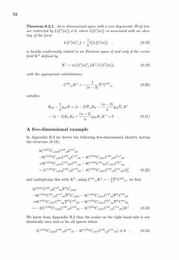
52
Theorem 8.2.1. An n-dimensional space with a non-degenerate Weyl ten-sor restricted by LC[m] 6= 0, where LC[m] is associated with an iden-tity of the form
LC[m]ij =1n
δijLC[m] , (8.18)
is locally conformally related to an Einstein space if and only if the vectorfield Ka defined by
Ki = nLC[m]ijKj/LC[m], (8.19)
with the appropriate substitutions
CabcjK
j = − 1(n− 3)
∇jCabcj (8.20)
satisfies
Rab − 1n
gabR + (n− 2)∇aKb − (n− 2)n
gab∇cKc
− (n− 2)KaKb +(n− 2)
ngabKcK
c = 0 . (8.21)
A five-dimensional example
In Appendix B.2 we derive the following five-dimensional identity havingthe structure (8.18),
5CijkfCijkhCabcdC
cdab
−8CijkgCijkhCabcgC
cfab − 4CijkgCijkeC
abghCef
ab
+8CijkgCijkeCaf
bhCbeag − 8CijkgCae
bhCijkeCbf
ag
= (CijkgCijkgCab
cdCcd
ab − 4CijkgCijkeCab
cgCce
ab)δfh (8.22)
and multiplying this with Kh, using CabcjK
j = − 12∇jCab
cj , we find
5CijkfCabcdC
cdab∇hCijkh
−8CijkgCabcgC
cfab∇hCijkh − 4CijkgCijkeC
efab∇hCab
gh
+8CijkgCijkeCbe
ag∇hCafbh − 8CijkgCijkeC
bfag∇hCae
bh
= −2(CijkgCijkgCab
cdCcd
ab − 4CijkgCijkeCab
cgCce
ab)Kf . (8.23)
We know from Appendix B.2 that the scalar on the right hand side is notidentically zero and so for all spaces where
(CijkgCijkgCab
cdCcd
ab − 4CijkgCijkeCab
cgCce
ab) 6= 0 , (8.24)
August 20, 2004 (15:33)
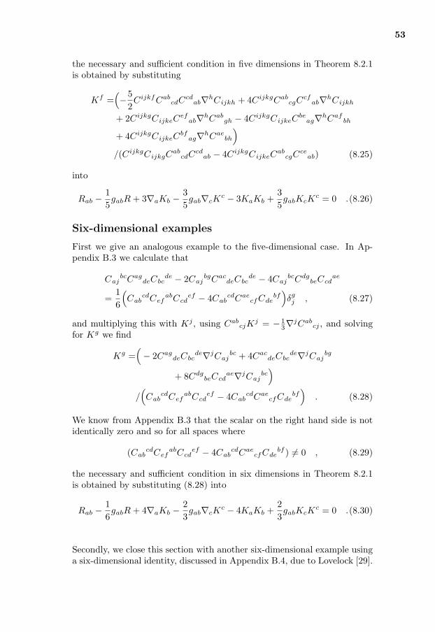
53
the necessary and sufficient condition in five dimensions in Theorem 8.2.1is obtained by substituting
Kf =(−5
2CijkfCab
cdCcd
ab∇hCijkh + 4CijkgCabcgC
cfab∇hCijkh
+ 2CijkgCijkeCef
ab∇hCabgh − 4CijkgCijkeC
beag∇hCaf
bh
+ 4CijkgCijkeCbf
ag∇hCaebh
)
/(CijkgCijkgCab
cdCcd
ab − 4CijkgCijkeCab
cgCce
ab) (8.25)
into
Rab − 15gabR + 3∇aKb − 3
5gab∇cK
c − 3KaKb +35gabKcK
c = 0 .(8.26)
Six-dimensional examples
First we give an analogous example to the five-dimensional case. In Ap-pendix B.3 we calculate that
CajbcCag
deCbcde − 2Caj
bgCacdeCbc
de − 4CajbcCdg
beCcdae
=16
(Cab
cdCefabCcd
ef − 4CabcdCae
cfCdebf
)δg
j , (8.27)
and multiplying this with Kj , using CabcjK
j = − 13∇jCab
cj , and solvingfor Kg we find
Kg =(− 2Cag
deCbcde∇jCaj
bc + 4CacdeCbc
de∇jCajbg
+ 8CdgbeCcd
ae∇jCajbc
)
/(Cab
cdCefabCcd
ef − 4CabcdCae
cfCdebf
). (8.28)
We know from Appendix B.3 that the scalar on the right hand side is notidentically zero and so for all spaces where
(CabcdCef
abCcdef − 4Cab
cdCaecfCde
bf ) 6= 0 , (8.29)
the necessary and sufficient condition in six dimensions in Theorem 8.2.1is obtained by substituting (8.28) into
Rab − 16gabR + 4∇aKb − 2
3gab∇cK
c − 4KaKb +23gabKcK
c = 0 .(8.30)
Secondly, we close this section with another six-dimensional example usinga six-dimensional identity, discussed in Appendix B.4, due to Lovelock [29].
August 20, 2004 (15:33)

54
This identity involves the tensor Aijkabc which is quadratic in the Weyl
tensor and defined by
Aijkabc = 4C [ij
h[aCk]hbc] . (8.31)
The analogous identity to (8.18) is (B.20),
AabicdeAcde
abj + 3AabiabcAcde
dej + 6AabiacdAcde
bej
− 3AabcadeAdei
bcj −AabcabcAdei
dej + 6AabcabdAdei
cej
+16Aabc
abcAdefdefδj
i +32Aabc
adeAdefbcfδj
i
− 32Aabc
abdAdefcefδj
i − 16Aabc
defAdefabcδj
i = 0, (8.32)
and multiplying by Ki and solving for Kj we have (provided we can performthe division)
Kj =6(KiAabi
cdeAcdeabj + 3KiAabi
abcAcdedej + 6KiAabi
acdAcdebej
− 3AabcadeKiAdei
bcj −AabcabcKiAdei
dej + 6AabcabdΥiAdei
cej)
/(AabcdefAdef
abc −AabcabcAdef
def
− 9AabcadeAdef
bcf + 9AabcabdAdef
cef ) . (8.33)
Hence in this case we get the necessary and sufficient condition in six di-mension in Theorem 8.2.1 by first substituting all the terms involving Ki
on the right hand side via
KiAiabcde = ∇iCi[a
p[cCb]pde] −∇iCip
[deCabc]p (8.34)
and all the other terms on the right hand side via
Aijkabc = 4C [ij
h[aCk]hbc] . (8.35)
into (8.33) and then this expression into
Rab − 16gabR + 4∇aKb − 2
3gab∇cK
c − 4KaKb +23gabKcK
c = 0 .(8.36)
August 20, 2004 (15:33)
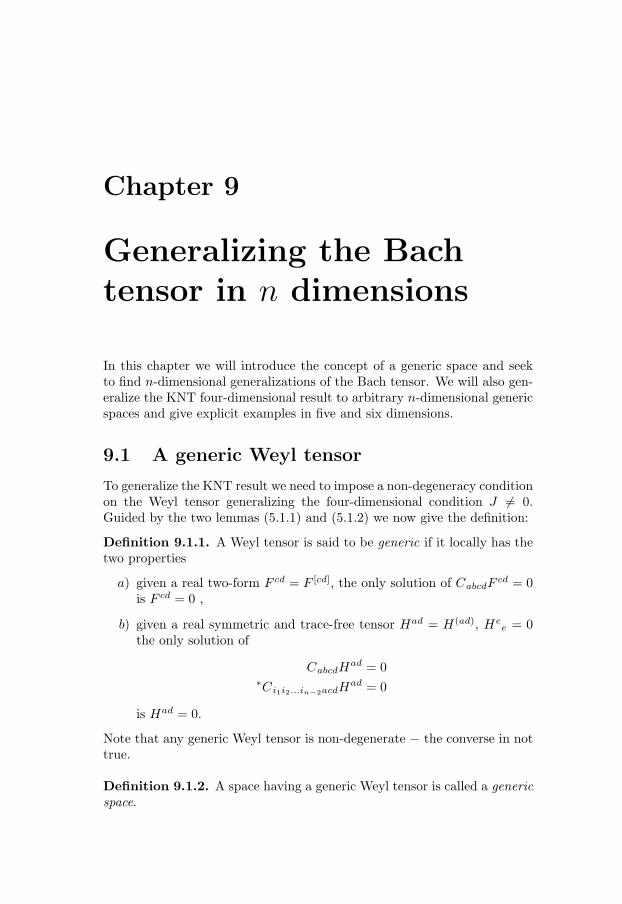
Chapter 9
Generalizing the Bachtensor in n dimensions
In this chapter we will introduce the concept of a generic space and seekto find n-dimensional generalizations of the Bach tensor. We will also gen-eralize the KNT four-dimensional result to arbitrary n-dimensional genericspaces and give explicit examples in five and six dimensions.
9.1 A generic Weyl tensor
To generalize the KNT result we need to impose a non-degeneracy conditionon the Weyl tensor generalizing the four-dimensional condition J 6= 0.Guided by the two lemmas (5.1.1) and (5.1.2) we now give the definition:
Definition 9.1.1. A Weyl tensor is said to be generic if it locally has thetwo properties
a) given a real two-form F cd = F [cd], the only solution of CabcdFcd = 0
is F cd = 0 ,
b) given a real symmetric and trace-free tensor Had = H(ad), Hee = 0
the only solution of
CabcdHad = 0
∗Ci1i2...in−2acdHad = 0
is Had = 0.
Note that any generic Weyl tensor is non-degenerate − the converse in nottrue.
Definition 9.1.2. A space having a generic Weyl tensor is called a genericspace.
August 20, 2004 (15:33)
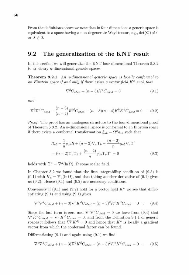
56
From the definitions above we note that in four dimensions a generic space isequivalent to a space having a non-degenerate Weyl tensor, e.g., det(C) 6= 0or J 6= 0.
9.2 The generalization of the KNT result
In this section we will generalize the KNT four-dimensional Theorem 5.3.2to arbitrary n-dimensional generic spaces.
Theorem 9.2.1. An n-dimensional generic space is locally conformal toan Einstein space if and only if there exists a vector field Ka such that
∇dCabcd + (n− 3)KdCabcd = 0 (9.1)
and
∇b∇dCabcd − (n− 3)(n− 2)
RbdCabcd − (n− 3)(n− 4)KbKdCabcd = 0 . (9.2)
Proof. The proof has an analogous structure to the four-dimensional proofof Theorem 5.3.2. An n-dimensional space is conformal to an Einstein spaceif there exists a conformal transformation gab = Ω2gab such that
Rab − 1n
gabR + (n− 2)∇aΥb − (n− 2)n
gab∇cΥc
− (n− 2)ΥaΥb +(n− 2)
ngabΥcΥc = 0 (9.3)
holds with Υa = ∇a(lnΩ), Ω some scalar field.
In Chapter 3.2 we found that the first integrability condition of (9.3) is(9.1) with Ka = ∇a(lnΩ), and that taking another derivative of (9.1) givesus (9.2). Hence (9.1) and (9.2) are necessary conditions.
Conversely if (9.1) and (9.2) hold for a vector field Ka we see that differ-entiating (9.1) and using (9.1) gives
∇c∇dCabcd + (n− 3)∇cKdCabcd − (n− 3)2KcKdCabcd = 0 . (9.4)
Since the last term is zero and ∇c∇dCabcd = 0 we have from (9.4) that∇cKdCabcd = ∇[cKd]Cabcd = 0, and from the Definition 9.1.1 of genericspaces it follows that ∇[cKd] = 0 and hence that Ka is locally a gradientvector from which the conformal factor can be found.
Differentiating (9.1) and again using (9.1) we find
∇b∇dCabcd + (n− 3)∇bKdCabcd − (n− 3)2KbKdCabcd = 0 . (9.5)
August 20, 2004 (15:33)
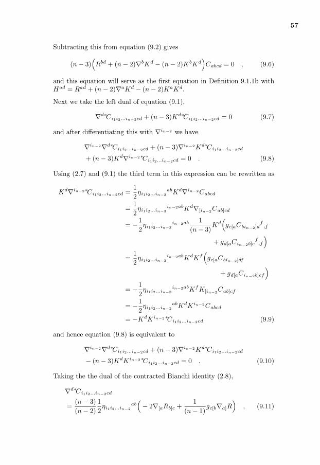
57
Subtracting this from equation (9.2) gives
(n− 3)(Rbd + (n− 2)∇bKd − (n− 2)KbKd
)Cabcd = 0 , (9.6)
and this equation will serve as the first equation in Definition 9.1.1b withHad = Rad + (n− 2)∇aKd − (n− 2)KaKd.
Next we take the left dual of equation (9.1),
∇d∗Ci1i2...in−2cd + (n− 3)Kd∗Ci1i2...in−2cd = 0 (9.7)
and after differentiating this with ∇in−2 we have
∇in−2∇d∗Ci1i2...in−2cd + (n− 3)∇in−2Kd∗Ci1i2...in−2cd
+ (n− 3)Kd∇in−2∗Ci1i2...in−2cd = 0 . (9.8)
Using (2.7) and (9.1) the third term in this expression can be rewritten as
Kd∇in−2∗Ci1i2...in−2cd =12ηi1i2...in−2
abKd∇in−2Cabcd
=12ηi1i2...in−3
in−2abKd∇[in−2Cab]cd
= −12ηi1i2...in−3
in−2ab 1(n− 3)
Kd(gc[aCbin−2]d
f;f
+ gd[aCin−2b]cf;f
)
=12ηi1i2...in−3
in−2abKdKf(gc[aCbin−2]df
+ gd[aCin−2b]cf
)
= −12ηi1i2...in−3
in−2abKfK[in−2Cab]cf
= −12ηi1i2...in−2
abKdKin−2Cabcd
= −KdKin−2∗Ci1i2...in−2cd (9.9)
and hence equation (9.8) is equivalent to
∇in−2∇d∗Ci1i2...in−2cd + (n− 3)∇in−2Kd∗Ci1i2...in−2cd
− (n− 3)KdKin−2∗Ci1i2...in−2cd = 0 . (9.10)
Taking the the dual of the contracted Bianchi identity (2.8),
∇d∗Ci1i2...in−2cd
=(n− 3)(n− 2)
12ηi1i2...in−2
ab(− 2∇[aRb]c +
1(n− 1)
gc[b∇a]R)
, (9.11)
August 20, 2004 (15:33)
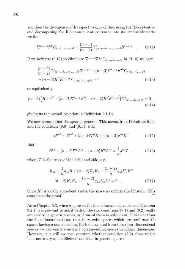
58
and then the divergence with respect to in−2 of this, using the Ricci identityand decomposing the Riemann curvature tensor into its irreducible partswe find
∇in−2∇d∗Ci1i2...in−2cd =(n− 3)(n− 2)
∗Ci1i2...in−3in−2cdRin−2d . (9.12)
If we now use (9.12) to eliminate ∇in−2∇d∗Ci1i2...in−2cd in (9.10) we have
(n− 3)(n− 2)
∗Ci1i2...in−3in−2cdRin−2d + (n− 3)∇in−2Kd∗Ci1i2...in−2cd
− (n− 3)KdKin−2∗Ci1i2...in−2cd = 0 (9.13)
or equivalently
(n− 3)(Rin−2d + (n− 2)∇in−2Kd − (n− 2)KdKin−2
)∗Ci1i2...in−2cd = 0 ,
(9.14)
giving us the second equation in Definition 9.1.1b.
We now assume that the space is generic. This means from Definition 9.1.1and the equations (9.6) and (9.14) with
Had = Rad + (n− 2)∇aKd − (n− 2)KaKd (9.15)
that
Rad + (n− 2)∇aKd − (n− 2)KaKd =1n
gadT , (9.16)
where T is the trace of the left hand side, e.g.,
Rab − 1n
gabR + (n− 2)∇aKb − (n− 2)n
gab∇cKc
− (n− 2)KaKb +(n− 2)
ngabKcK
c = 0 . (9.17)
Since Ka is locally a gradient vector the space is conformally Einstein. Thiscompletes the proof.
As in Chapter 5.3, when we proved the four-dimensional version of Theorem9.2.1, it is relevant to ask if both of the two conditions (9.1) and (9.2) reallyare needed in generic spaces, or if one of them is redundant. It is clear fromthe four-dimensional case that there exist spaces which are conformal C-spaces having a non-vanishing Bach tensor, and from these four-dimensionalspaces we can easily construct corresponding spaces in higher dimension.However, it is still an open question whether condition (9.2) alone mightbe a necessary and sufficient condition in generic spaces.
August 20, 2004 (15:33)
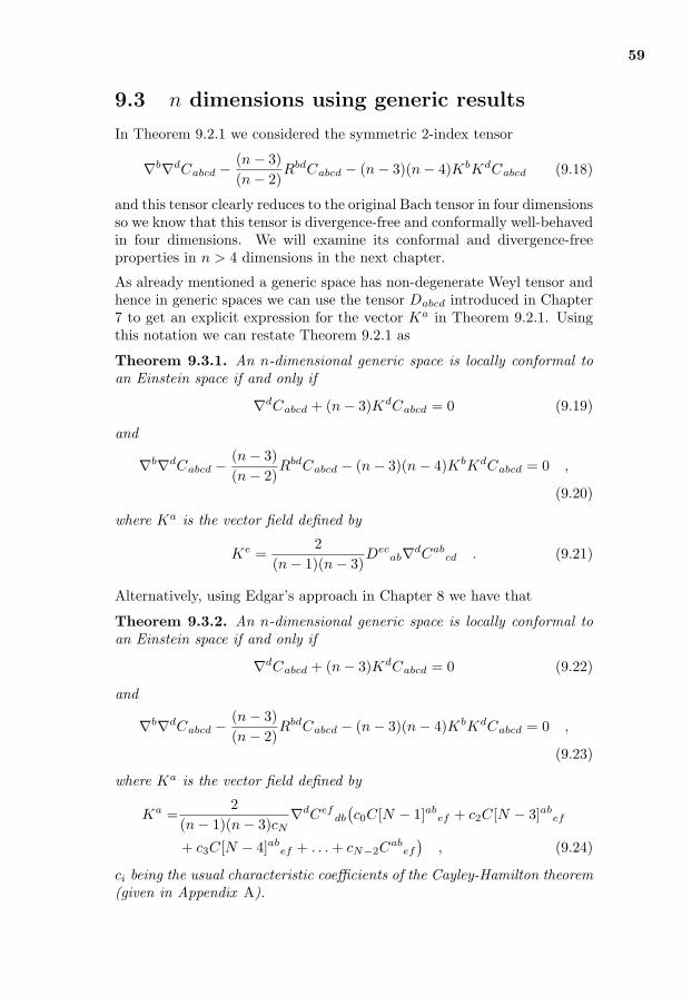
59
9.3 n dimensions using generic results
In Theorem 9.2.1 we considered the symmetric 2-index tensor
∇b∇dCabcd − (n− 3)(n− 2)
RbdCabcd − (n− 3)(n− 4)KbKdCabcd (9.18)
and this tensor clearly reduces to the original Bach tensor in four dimensionsso we know that this tensor is divergence-free and conformally well-behavedin four dimensions. We will examine its conformal and divergence-freeproperties in n > 4 dimensions in the next chapter.
As already mentioned a generic space has non-degenerate Weyl tensor andhence in generic spaces we can use the tensor Dabcd introduced in Chapter7 to get an explicit expression for the vector Ka in Theorem 9.2.1. Usingthis notation we can restate Theorem 9.2.1 as
Theorem 9.3.1. An n-dimensional generic space is locally conformal toan Einstein space if and only if
∇dCabcd + (n− 3)KdCabcd = 0 (9.19)
and
∇b∇dCabcd − (n− 3)(n− 2)
RbdCabcd − (n− 3)(n− 4)KbKdCabcd = 0 ,
(9.20)
where Ka is the vector field defined by
Ke =2
(n− 1)(n− 3)Dec
ab∇dCabcd . (9.21)
Alternatively, using Edgar’s approach in Chapter 8 we have that
Theorem 9.3.2. An n-dimensional generic space is locally conformal toan Einstein space if and only if
∇dCabcd + (n− 3)KdCabcd = 0 (9.22)
and
∇b∇dCabcd − (n− 3)(n− 2)
RbdCabcd − (n− 3)(n− 4)KbKdCabcd = 0 ,
(9.23)
where Ka is the vector field defined by
Ka =2
(n− 1)(n− 3)cN∇dCef
db
(c0C[N − 1]ab
ef + c2C[N − 3]abef
+ c3C[N − 4]abef + . . . + cN−2C
abef
), (9.24)
ci being the usual characteristic coefficients of the Cayley-Hamilton theorem(given in Appendix A).
August 20, 2004 (15:33)
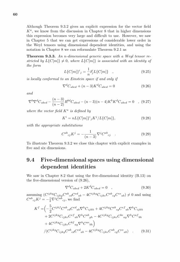
60
Although Theorem 9.3.2 gives an explicit expression for the vector fieldKa, we know from the discussion in Chapter 8 that in higher dimensionsthis expression becomes very large and difficult to use. However, we sawin Chapter 5 that we can get expressions of considerable lower order inthe Weyl tensors using dimensional dependent identities, and using thenotation in Chapter 8 we can reformulate Theorem 9.2.1 as
Theorem 9.3.3. An n-dimensional generic space with a Weyl tensor re-stricted by LC[m] 6= 0, where LC[m] is associated with an identity ofthe form
LC[m]ij =
1n
δijLC[m] , (9.25)
is locally conformal to an Einstein space if and only if
∇dCabcd + (n− 3)KdCabcd = 0 (9.26)
and
∇b∇dCabcd − (n− 3)(n− 2)
RbdCabcd − (n− 3)(n− 4)KbKdCabcd = 0 , (9.27)
where the vector field Ka is defined by
Ki = nLC[m]ijK
j/LC[m], (9.28)
with the appropriate substitutions
CabcjK
j = − 1(n− 3)
∇jCabcj . (9.29)
To illustrate Theorem 9.3.2 we close this chapter with explicit examples infive and six dimensions.
9.4 Five-dimensional spaces using dimensionaldependent identities
We saw in Chapter 8.2 that using the five-dimensional identity (B.13) onthe five-dimensional version of (9.26),
∇dCabcd + 2KdCabcd = 0 , (9.30)
assuming (CijkgCijkgCab
cdCcd
ab − 4CijkgCijkeCab
cgCce
ab) 6= 0 and usingCab
cjKj = − 1
2∇jCabcj , we find
Kf =(−5
2CijkfCab
cdCcd
ab∇hCijkh + 4CijkgCabcgC
cfab∇hCijkh
+ 2CijkgCijkeCef
ab∇hCabgh − 4CijkgCijkeC
beag∇hCaf
bh
+ 4CijkgCijkeCbf
ag∇hCaebh
)
/(CijkgCijkgCab
cdCcd
ab − 4CijkgCijkeCab
cgCce
ab) . (9.31)
August 20, 2004 (15:33)

61
Hence the necessary and sufficient condition for a five-dimensional genericspace with (CijkgCijkgC
abcdC
cdab−4CijkgCijkeC
abcgC
ceab) 6= 0 to be con-
formally related to an Einstein space is that
∇dCabcd + 2KdCabcd = 0 (9.32)
and∇b∇dCabcd − 2
3RbdCabcd − 2KbKdCabcd = 0 (9.33)
hold, where Ka is given by (9.31).
9.5 Six-dimensional spaces using dimensionaldependent identities
In six dimensions, equation (9.26) become
∇dCabcd + 3KdCabcd = 0 , (9.34)
and, as in Chapter 8.2, after the use of the six-dimensional dependentidentity (B.15) and Cab
cjKj =−1
3∇jCabcj , we find that
Kg =− 2CagdeCbc
de∇jCajbc + 4Cac
fdeCbcde∇jCaj
bg
+ 8CdgbeCcd
ae∇jCajbc
/(CabcdCef
abCcdef − 4Cab
cdCaecfCde
bf ) , (9.35)
providing (CijkgCijkgCab
cdCcd
ab − 4CijkgCijkeCab
cgCce
ab) 6= 0.
So, a six-dimensional generic space, in which the scalar
(CijkgCijkgCab
cdCcd
ab − 4CijkgCijkeCab
cgCce
ab) 6= 0 (9.36)
is conformally related to an Einstein space if and only if
∇dCabcd + 3KdCabcd = 0 (9.37)
and∇b∇dCabcd − 3
4RbdCabcd − 6KbKdCabcd = 0 (9.38)
hold, where Ka is given by (9.35).
August 20, 2004 (15:33)

Chapter 10
Conformal properties ofdifferent tensors
In Chapter 4 we showed that some obvious attempts for an n-dimensionalgeneralization of the Bach tensor were not conformally well-behaved nordivergence-free in dimensions n > 4. Now we have found another general-ization of this tensor, Bac,
Bac = ∇b∇dCabcd − (n− 3)(n− 2)
RbdCabcd − (n− 3)(n− 4)KbKdCabcd (10.1)
with important properties, and in this chapter we will investigate conformalproperties of this and related tensors.
10.1 The tensors babc and Bac and their con-formal properties in generic spaces
The tensor Bac is, as the original four-dimensional Bach tensor Bac, moti-vated by the second integrability condition for a space being conformal toan Einstein space; it is found by taking a derivative of
∇dCabcd + (n− 3)KdCabcd = 0 (10.2)
and is given by
Bac = ∇b∇dCabcd − (n− 3)(n− 2)
RbdCabcd − (n− 3)(n− 4)KbKdCabcd = 0 ,
(10.3)
where we replaced the vector field Υa connected with a conformal trans-formation with the vector field Ka.
August 20, 2004 (15:33)
63
In general we cannot discuss the conformal properties of the form (10.3)for Bac because of the non-geometric vector Ka. However, we encounteredBac as one of the two sufficient and necessary conditions for a space to beconformal to an Einstein space, so we look at these two conditions togetherand check their conformal behavior.
In a space with non-degenerate Weyl tensor let us define the vector fieldKG
a by
KG
a =2
(n− 1)(n− 3)Dai
jk∇dCjkid , (10.4)
where Dabcd is the tensor satisfying
DabcdC
cdef = δa
[eδbf ] . (10.5)
Hence, in a space with non-degenerate Weyl tensor, guided by (10.2), wewill define
babc = ∇dCabcd + KG
dCabcd
= ∇dCabcd +2
(n− 1)CabcdD
dijk∇lCjk
il (10.6)
and, guided by Bac in (10.3) we define,
Bac =∇b∇dCabcd − (n− 3)(n− 2)
RbdCabcd − (n− 3)(n− 5)KG
bKG
dCabcd
=∇b∇dCabcd − (n− 3)(n− 2)
RbdCabcd
− 4(n− 4)(n− 1)2(n− 3)
Dbijk∇lCjk
ilDdr
pq∇mCpqrmCabcd . (10.7)
Since the right hand side of equation (10.5) is conformally invariant undera conformal transformation gab = Ω2gab, we have
δa[eδ
bf ] = Dab
cdCcd
ef = Ω−2DabcdC
cdef , (10.8)
and multiplying this with Defgh, solving for Dab
cd, we find that the con-formal behavior of Dab
cd is
Dabcd = Ω2Dab
cd . (10.9)
Using (10.5) and the conformal property of Dabcd as well as the well-known
August 20, 2004 (15:33)
64
ones for the Weyl tensor we see that the conformal behavior of babc is
babc = ∇dCabcd +2
(n− 1)CabcdD
dijk∇lCjk
il
= ∇dCabcd + (n− 3)ΥdCabcd
+2
(n− 1)CabcdD
dijk
(∇lCjk
il + (n− 3)ΥlCjkil
)
= ∇dCabcd +2
(n− 1)CabcdD
dijk∇lCjk
il
+ (n− 3)ΥdCabcd +2(n− 3)(n− 1)
ΥlCabcdDdi
jkCjkil
= babc , (10.10)
i.e., that babc is conformally invariant.
Turning to the tensor Bbc we find after some calculation that under aconformal transformation gab = Ω2gab, we have
Bac = Ω−2Bac + (n− 4)Ω−2
(Υb
(Cabcd;
d + (n− 3)KdCabcd
)
+ Υd(Cabcd;
b + (n− 3)KbCabcd
)), (10.11)
meaning that in general Bbc is not conformally well-behaved.
However, in a space with non-degenerate Weyl tensor we can use (10.6) torewrite (10.11) as
Bac = Ω−2Bac + (n− 4)Ω−2
(Υbbabc + Υdbacd
), (10.12)
and it is clear from (10.12) that under the condition that babc = 0 we seethat Bbc is in fact conformally weighted with weight −2. We collect theseresults in the following theorem:
Theorem 10.1.1. In a space with non-degenerate Weyl tensor the tensor
babc = ∇dCabcd +2
(n− 1)CabcdD
dijk∇lCjk
il (10.13)
is conformally invariant but the tensor
Bac =∇b∇dCabcd − (n− 3)(n− 2)
RbdCabcd
− 4(n− 4)(n− 1)2(n− 3)
Dbijk∇lCjk
ilDdr
pq∇mCpqrmCabcd (10.14)
is in general not. However, if babc = 0, then Bbc is conformally weightedwith weight −2.
August 20, 2004 (15:33)
65
Note that, remembering that generic spaces are subspaces of the class ofspaces with non-degenerate Weyl tensor, and using the notation (10.6) and(10.7) we can reformulate the sufficient and necessary condition for a spacebeing conformal to an Einstein space, i.e., Theorem (9.2.1), as
Theorem 10.1.2. A generic space is conformal to an Einstein space ifand only if the conformal invariant condition hold,
babc = 0 (10.15)
and
Bbc = 0 . (10.16)
10.2 The tensor Lab and its conformal prop-erties
Motivated by Listing’s n-dimensional result (Theorem (7.3.2)) we will de-fine, in a space with non-degenerate Weyl tensor, the tensor
Lab =Rab − 1n
gabR + (n− 2)∇aKG
b +(n− 2)
ngab∇cK
G
c
− (n− 2)KG
aKG
b +(n− 2)
ngabK
GcK
G
c , (10.17)
where KG
a is defined by (10.4) .
Hence, in a space with non-degenerate Weyl tensor, the tensor Lab is builtup purely from geometry, and we find that under a conformal transforma-tion gab = Ω2gab, using
KG
e=
2(n− 1)(n− 3)
Decab∇dCab
cd
=2
(n− 1)(n− 3)Dec
ab
(∇dCab
cd + (n− 3)ΥdCabcd
)
=2
(n− 1)(n− 3)Dec
ab∇dCabcd + Υd 2
(n− 1)Dec
abCab
cd
= KG
e −Υe , (10.18)
August 20, 2004 (15:33)

66
that
Lab = Rab − 1n
gabR + (n− 2)∇aKG
b − (n− 2)n
gab∇cKG
c
− (n− 2)KG
aKG
b +(n− 2)
ngabK
GcK
G
c
= Rab + (n− 2)∇aΥb + gab∇cΥc − (n− 2)ΥaΥb + (n− 2)gabΥcΥc
− 1n
gab
(R + 2(n− 1)∇cΥc + (n− 1)(n− 2)ΥcΥc
)
+ (n− 2)(∇aK
Gb −∇aΥb − 2K
G(aΥb) + 2ΥaΥb + gabΥc
(KG
c −Υc
))
− (n− 2)n
gab
(∇cK
G
c −∇cΥc + (n− 2)ΥcKG
c − (n− 2)ΥcΥc)
− (n− 2)(KG
a−Υa
)(KG
b−Υb
)+
(n− 2)n
gab
(KG
c−Υc
)(KG
c−Υc)
= Lab , (10.19)
i.e., that Lab is conformally invariant, and we have
Theorem 10.2.1. In a space with non-degenerate Weyl tenor, the tensorLab defined by equation (10.17), with all the K
G
a substituted using (10.4), is
conformally invariant.
August 20, 2004 (15:33)
Chapter 11
Concluding remarks andfuture work
In this thesis we began by reviewing the developments of the problem offinding necessary and sufficient conditions for a space to be conformal toan Einstein space.Since the Bach tensor featured in some four-dimensional results, we lookedto see if there was an obvious n-dimensional analogue of the Bach tensor.A theorem due to Belfagon and Jean was strengthened and a basis, con-sisting of three tensors, for all n-dimensional symmetric, divergence-free2-index tensors which are also quadratic in the Riemann curvature tensor,was presented. We were able to show that the Bach tensor is a linear com-bination of these tensors in four dimensions, and that the Bach tensor isthe only (up to constant rescaling) 2-index tensor in four dimensions whichis symmetric, divergence-free, conformally well-behaved, and quadratic inthe Riemann curvature tensor; however, there was no such n-dimensionalresult. Specifically, we have shown for dimensions n > 4, in general, thatthere is no 2-index symmetric and divergence-free tensor quadratic in theRiemann curvature tensor which is also of good conformal weight.So rather than focus on a generalization of the Bach tensor itself we lookedfor a generalization of the four-dimensional KNT result, which providedtwo necessary and sufficient conditions (one of which involves the Bachtensor) for the existence of conformal Einstein spaces.We have introduced the concept of a generic Weyl tensor and a genericspace, which is stronger than the KNT condition J 6= 0, and so we wereable to generalize the KNT four-dimensional result to n dimensions, n ≥ 4.We found that a generic space is locally conformal to an Einstein space ifand only if two conformally invariant conditions hold:
babc = 0 (11.1)
August 20, 2004 (15:33)
68
and
Bab = 0 . (11.2)
The tensor Bab in a sense generalizes the Bach tensor Bab to n dimensions.We have also shown that the tensors babc and Lab are conformally invariantin spaces with non-degenerate Weyl tensor, and that for spaces in whichbabc = 0 the tensor Bab is conformally weighted with weight −2.Explicit examples of these new results have been given in four, five andsix dimensions using (in the five- and six-dimensional cases) newly derivedtensor identities.As well as obtaining a number of new identities in Appendix B, we alsofound in Appendix C the explicit relation between the two complex scalarinvariants of the Weyl spinor and four real invariants of the Weyl tensor.
There are some questions that would be interesting to address in the future.We have already mentioned that a generic Weyl tensor also is a non-degenerate Weyl tensor, but not vice-versa1. The natural questions arise:what is the difference between these two, and how much bigger is the class ofspaces having non-degenerate Weyl tensor compared to the class of genericspaces? Is there a way to extend the results for the generic class so thatthey apply to the larger class of spaces having non-degenerate Weyl tensor?Is there a way of extending such results even to a larger class than the classof spaces having non-degenerate Weyl tensor, i.e., to spaces where J = 0.We have pointed out that the question of whether Bab = 0 in a spacehaving non-degenerate Weyl tensor in four dimension is alone a necessarycondition for conformal Einstein spaces is still open. We suspect it is notso, and it would be good to find a precise counterexample.We have not distinguished between positive definite and Lorentz metrics;it would appear that when we make this distinction we can get strongerresults for the positive definite cases. The Lorentz case is well covered infour dimensions, but not in higher dimensions. The conditions put on theWeyl tensor in four dimensions are related to the Petrov classification, butin n dimensions, n > 4, no such classification is known. However, recentlyColey, Milson, Pravda and Pravdova [8], [9], [10] developed a classificationof the Weyl tensor in higher dimension using aligned null vectors of variousorders of alignment. It would be interesting to see how the conditions fora generic space look in their formalism, and if their formalism gives rise toother natural necessary and sufficient conditions in higher dimensions.Finally, we note that the very recent work of Gover and Nurowski [16]offers wider possibilities within differential geometry; an obvious next stepis to try and exploit our new identities in higher dimensions within thesedevelopments.
1In four dimensions they are equivalent.
August 20, 2004 (15:33)
Appendix A
The Cayley-HamiltonTheorem and thetranslation of the Weyltensor/spinor to a matrix
In this appendix we will review the Cayley-Hamilton Theorem and see howwe can translate the Wely tensor and/or the Weyl spinor to a matrix. Wewe also formulate the Cayley-Hamilton Theorem in tensor notation.
A.1 The Cayley-Hamilton Theorem
The Cayley-Hamilton Theorem1 states that a matrix satisfies its character-istic polynomial, i.e., for a n× n matrix A with characteristic polynomial
p(x) = a0xn + a1x
n−1 + . . . + an−1x + an , (A.1)
p(A) = 0.
It is a well-know fact [19], [38] that the relation between the determinantof a n× n matrix A and the coefficient an in its characteristic polynomialis
(−1)n det(A) = an . (A.2)
A linear transformation on an n-dimensional vector space V given by ann× n matrix A can be interpreted as a tensor Aa
b and vice-versa. In thiscontext the Cayley-Hamilton Theorem can be written
Ac1[c1A
c2c2 · · ·Acn−1
cn−1Acn
cnδab] = 0 , (A.3)
1See [38] for a general proof.
August 20, 2004 (15:33)
70
i.e., as a consequence of antisymmetrising over n + 1 indices, and one cancalculate the coefficients a1, a2, . . . , an of the characteristic polynomial interms of traces of the matrix from
ak = A[i1i1A
i2i2 . . . Aik]
ik, k = 1 . . . n (A.4)
(a0=1).
So, for an n× n matrix A the Cayley-Hamilton Theorem is given by
a0An + a1An−1 + a2An−2 + . . . + an−2A2 + an−1A + anI = 0 , (A.5)
where I is the n × n identity matrix, and denoting the trace of a matrixwith square brackets the characteristic coefficients are given by [19]
a0 = 1, a1 = −[A], a2 = −12
([A2]−
([A]
)2)
,
a3 = − 13!
(2[A3]− 3[A][A2] +
([A]
)3)
,
a4 = − 14!
(6[A4]− 3
([A2]
)2
− 8[A][A3] + [A2]([A]
)2
−([A]
)4)
,
. . . ,
an = − 1n!
((n− 1)![An] + . . . + . . .
). (A.6)
Note that if the matrix is trace-free we will have [A] = 0 in the expressionsfor the coefficients ak above, and especially, a1 = 0.
For future reference we write out two special cases of particular interest forus.
The case where n = 3 and the matrix is trace-free.
In the case of a 3 × 3 trace-free matrix A the Cayley-Hamilton Theorembecomes
a0A3 + a2A + a3I = 0 , (A.7)
wherea0 = 1, a2 = −1
2[A2], a3 = −1
3[A3] , (A.8)
i.e.,
A3 − 12[A2]A− 1
3[A3]I = 0 . (A.9)
The determinant in terms of traces of A is
det(A) =13[A3] . (A.10)
August 20, 2004 (15:33)
71
The case where n = 6 and the matrix is trace-free.
In the case of a 6 × 6 trace-free matrix A the Cayley-Hamilton Theoremstates
a0A6 + a2A4 + a3A3 + a4A2 + a5A + a6I = 0 , (A.11)
where
a0 = 1, a2 = −12[A2], a3 = −1
3[A3],
a4 = −14
([A4]− 1
2
([A2]
)2)
, a5 = −15
([A5]− 5
6[A2][A3]
),
a6 = −16
([A6]− 3
4[A2][A4]− 1
3
([A3]
)2
+18
([A2]
)3)
. (A.12)
The formula expressing the determinant of A in terms of traces is then
det(A) = −16
([A6]− 3
4[A2][A4]− 1
3
([A3]
)2
+18
([A2]
)3)
. (A.13)
A.2 Translation of Cabcd to a matrix CA
B
The n-dimensional Weyl tensor can be translated to a N × N trace-freematrix, where N = n(n− 1)/2. We write this as
CAC = Cab
cd , (A.14)
where A = [ab] and C = [cd] so that A, C = 1, 2, . . . , N . In doing thiswe only use the fact that the Weyl tensor is a double two-form, i.e., thatCab
cd = C [ab][cd], not the other symmetries, Cab
cd = Ccdab and C [abc]d = 0.
Also note that, in this construction, we are not defining a metric for theN -dimensional space.
In the case of n = 6, the Cayley-Hamilton Theorem applied to C gives
C6 − 12[C2]C5 − 1
3[C3]C4
− 14
([C4]− 1
2
([C2]
)2)
C3 − 15
([C5]− 5
6[C2][C3]
)C
− 16
([C6]− 3
4[C2][C4]− 1
3
([C3]
)2
+18
([C2]
)3)
I = 0 , (A.15)
August 20, 2004 (15:33)
72
and from (A.13) we have
det(C) = −16
([C6]− 3
4[C2][C4]− 1
3
([C3]
)2
+18
([C2]
)3)
. (A.16)
In four dimensions on the other hand, there is a more efficient represen-tation of the Weyl tensor using duals. In this case the Weyl tensor canbe represented via the trace-free complex 3 × 3 matrix C representingCab
cd + i∗Cabcd, where ∗Cab
cd = 12ηabijCijcd is the left dual of the Weyl
tensor.
So, in four dimensions, the Cayley-Hamilton Theorem (A.9) applied to thetrace-free matrix C gives
C3 − 12[C2]C − 1
3[C3]I = 0 (A.17)
and according to (A.10), the determinant in terms of traces of C is
det(C) =13[C3] . (A.18)
A.3 Translation of ΨABCD to a matrix Ψ
In four dimensions we can represent the Weyl spinor as a complex ma-trix, and this is done in detail in for instance [33]. The information of theWeyl tensor Cabcd in spinor languages is described by the fully symmet-ric Weyl spinor ΨABCD = Ψ(ABCD), and writing the Weyl spinor in theform ΨAB
CD we may regard it as a linear transformation on the (three-dimensional) complex space of symmetric spinors φAB = φ(AB),
φAB → ΨABCDφCD , (A.19)
and hence, analogous to the previous sections, can be described by a 3× 3complex matrix Ψ.
Looking at the eigenvalue problem for the mapping (A.19),
ΨABCDφCD = λφAB , (A.20)
we see by expressing (A.20) in components with respect to a specific basis2
that an eigenvalue λ of equation (A.20) also is an eigenvalue in the ordinary
2See [33] for details
August 20, 2004 (15:33)
73
sense of the matrix Ψ. Given that λ1, λ2 and λ3 are the three eigenvaluesof Ψ we have
λ1 + λ2 + λ3 = ΨABAB = 0 (A.21)
λ21 + λ2
2 + λ23 = ΨAB
CDΨCDAB = I (A.22)
λ31 + λ3
2 + λ33 = ΨAB
CDΨCDEF ΨEF
AB = J (A.23)
where I and J are the two complex scalar invariants of the Weyl spinor.By cubing (A.21) and subtracting 3 times the product of (A.21) and (A.22)we get
J = 3λ1λ2λ3 , (A.24)
i.e., that
det(Ψ) =13J . (A.25)
We note that the Weyl spinor has therefore two complex or four real inde-pendent scalar invariants. This result can be transfered to the Weyl tensor,where a direct proof is more complicated.
August 20, 2004 (15:33)

Appendix B
Dimensionally dependenttensor identities
The dimensionally dependent tensor identities are a class of identities basedon the trivial idea that antisymmetrising a tensor expression over moreindices than the number of dimensions makes the expression vanish.
In the late 1960’s Lovelock [29] studied some apparently unrelated tensoridentities and showed that they where all special cases of two dimensionallydependent identities. Lovelocks results have been generalized by Edgar andHoglund [14] and they proved the following theorem:
Theorem B.0.1. Let T a1...akb1...bm be antisymmetric in the upper and
lower indices respectively and d = n− k −m + 1 ≥ 0. Then
0 = T [a1...kk
[b1...bmδbm+1ak+1
. . . δbm+d]ak+d] ⇐⇒ T a1...ak
b1...bm is trace-free.
We will use this basic theorem to derive dimensionally dependent identitiessuitable for our purpose. Although the process of deriving these identitiesresults in a vast number of identities, only those relevant for us will beaccounted for here.
B.1 Four-dimensional identities
Theorem B.0.1 tells us that for the trace-free Weyl tensor Cabcd in four
dimensions, we haveC [ab
[cdδi]j] = 0 . (B.1)
Expanding the left hand side and using the antisymmetry of C gives
0 = Cabcdδ
ij − Cab
jdδic − Cab
cjδid
+Cbicdδ
aj + Cai
jdδbc − Cib
jcδa
d
+Ciacdδ
bj + Cib
jdδa
c + Ciajcδ
bd .
August 20, 2004 (15:33)

75
Multiplication by Ccdab and using the trace-free properties of the Weyl
tensor yields the well-know four-dimensional identity
CibcdCjbcd =14δijC
abcdCabcd . (B.2)
Using this identity (B.2) we can multiply (B.1) by CabefCef
cd and thensimplify this to
CibcdC
cdefCef
jb =14δijC
abcdC
cdefCef
ab . (B.3)
We can also in a similar manner derive the identities
∗CibcdCjbcd =14δij∗CabcdCabcd , (B.4)
∗Cibcd∗Ccd
ef∗Cef
jb =14δij∗Cab
cd∗Ccd
ef∗Cef
ab , (B.5)
starting with the dual version of (B.1).
Note that the scalars on the right of the equations (B.2) - (B.5) are fourreal invariants of the Weyl tensor [33]; since these are independent they canbe chosen as the basis for the invariants.
Also note that (B.2) is the only identity with two free indices one canconstruct from (B.1) involving a product of two Weyl tensors.
B.2 Five-dimensional identities
In five dimensions, from Theorem B.0.1, the analogue to (B.1) is
C [ab[cdδ
ehδ
f ]i] = 0 , (B.6)
which has eight free indices. Note that our“five-dimensional identity” (B.6)is also valid for four dimensions and that clearly we cannot get a quadraticexpression for Cab
cd involving only two free indices.
The only identity with two free indices cubic in the Weyl tensor is given by
CabpeC
gpcdC [ab
[cdδegδ
f ]h] = 0 . (B.7)
Expanding, collecting, and using the trace-free property gives
CafbcC
bcdeC
deah − 2Caf
bhCbcdeC
deac − 4Caf
bcCbd
ehCcead
=15
(Cab
cdCcd
egCeg
ab − 4CabcdC
ceagC
dgbe
)δf
h (B.8)
and the structures of (B.8) and (B.2) appear to be analogous. However, itturns out that the right hand side of (B.7) is identically zero for n ≤ 5. This
August 20, 2004 (15:33)
76
can be realized by looking at the five-dimensional scalar identity closelyrelated to (B.7)
CabcdC
ghefC [ab
[cdδegδ
f ]h] = 0 , (B.9)
which gives1
4CabcdC
ceafCdf
be = CabcdC
cdefCef
ab . (B.10)
Since we are interested in an identity with two free indices this case is notuseful for our purpose.
Nevertheless we note that (B.8) and (B.10) yields an interesting 2-indexfive-dimensional identity which will be useful in other contexts,
CafbcC
bcdeC
deah−2Caf
bhCbcdeC
deac−4Caf
bcCbd
ehCcead = 0 . (B.11)
On the other hand, if we consider a quartic identity in five dimensions,
CijkgCijkeCab
cdC [ab[cdδe
gδf ]h] = 0 , (B.12)
we obtain
5CijkfCijkhCabcdC
cdab
−8CijkgCijkhCabcgC
cfab − 4CijkgCijkeC
abghCef
ab
+8CijkgCijkeCaf
bhCbeag − 8CijkgCae
bhCijkeCbf
ag
= (CijkgCijkgCab
cdCcd
ab − 4CijkgCijkeCab
cgCce
ab)δfh . (B.13)
which again appears to have analogous structure to (B.2). To determine ifthe right hand side of (B.13) is identically zero, one could either look onall of the quartic scalar identities or try to find a counter example. Unlikein the cubic case where there was only one possible scalar identity (B.10),there will be a number of quartic scalar identities in five dimensions, sorather than starting to find all quartic scalar identities, a simple counterexample2 shows that the right hand side cannot be identically zero.
B.3 Six-dimensional identities
In six dimensions, from Theorem B.0.1, the analogue to (B.1) and (B.6) is
C [ab[cdδ
ehδf
i δg]j] = 0 (B.14)
1This five-dimensional scalar identity was also noted in [24], where it was obtainedfrom the five-dimensional identity Cab
[cdCcdef Cef
ab] = 0.2Using the Maple package GRTensorII [18] with the metric
ds2 = dr2
1− 12m
−Λr23 + e2
r2
+ r2dθ2 + r2 sin2(θ)dφ2 −(1− 1
2m− Λr2
3+ e2
r2
)dt2 + dx2
provides such a counterexample.
August 20, 2004 (15:33)
77
and this expression has 10 free indices. Hence there is only one possibilityto create an identity with two free indices involving three Weyl tensors.Expanding (B.14) and multiplying with Cab
cdCefhi we get
CajbcCag
deCbcde − 2Caj
bgCacdeCbc
de − 4CajbcCdg
beCcdae
=16
(Cab
cdCefabCcd
ef − 4CabcdCae
cfCdebf
)δg
j . (B.15)
Unlike for the case of the five-dimensional 2-index identity (B.8), there isno related scalar identity cubic in the Weyl tensor, analogous to (B.9).So therefore we do not need to worry about the possibility of the righthand side of (B.15) being identically zero, but we confirm this fact bya counterexample3, and so we have an identity which has precisely thestructure (B.2).
B.4 Lovelock’s quartic six-dimensional iden-tity
There are few explicit examples in the literature of identities for the Weyltensor in higher dimensions, but in the original paper [29] introducing di-mensionally dependent identities Lovelock gives an explicit example of asix-dimensional 2-index tensor identity quartic in the Weyl tensor. It in-volves the double three-form, Habc
efg,
Habcdef = H [abc]
[def ] ,
Habcdec = 0 , (B.16)
which in six dimensions (and lower) satisfies the identity
HabidefHdef
abj =16δji Habc
defHdefabc . (B.17)
Making the choice
Hijkabc =Aijk
abc − 94(n− 4)
Ar[jkr[bcδa]
i]
+18
(n− 4)(n− 3)Ars[i
rs[cδajδ
b]k]
+6
(2− n)(3− n)(4− n)Arst
rstδ[a[iδ
bjδ
c]k] (B.18)
3Again, using Maple and GRTensorII [18] with the metric
ds2 = dr2
1− 12m
−Λr23 + e2
r2
+ r2dθ2 + r2 sin2(θ)dφ2 −(1− 1
2m− Λr2
3+ e2
r2
)dt2 + dx2 + dy2
provides such a counterexample.
August 20, 2004 (15:33)
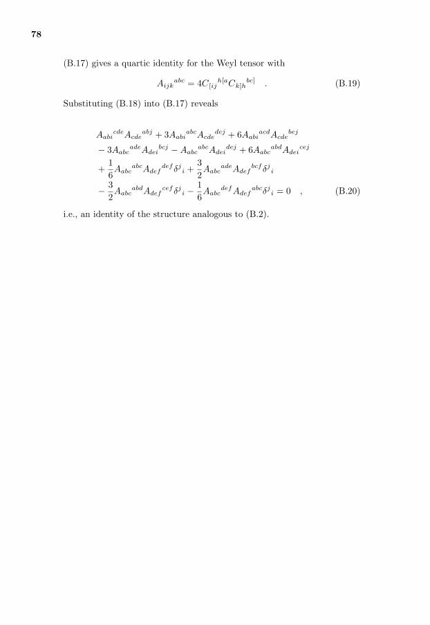
78
(B.17) gives a quartic identity for the Weyl tensor with
Aijkabc = 4C [ij
h[aCk]hbc] . (B.19)
Substituting (B.18) into (B.17) reveals
AabicdeAcde
abj + 3AabiabcAcde
dej + 6AabiacdAcde
bej
− 3AabcadeAdei
bcj −AabcabcAdei
dej + 6AabcabdAdei
cej
+16Aabc
abcAdefdefδj
i +32Aabc
adeAdefbcfδj
i
− 32Aabc
abdAdefcefδj
i − 16Aabc
defAdefabcδj
i = 0 , (B.20)
i.e., an identity of the structure analogous to (B.2).
August 20, 2004 (15:33)
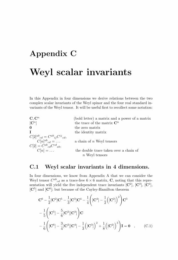
Appendix C
Weyl scalar invariants
In this Appendix in four dimensions we derive relations between the twocomplex scalar invariants of the Weyl spinor and the four real standard in-variants of the Weyl tensor. It will be useful first to recollect some notation:
C,Cn (bold letter) a matrix and a power of a matrix[Cn] the trace of the matrix Cn
0 the zero matrixI the identity matrixC[2]ab
cd = CabijC
ijcd,
C[n]abcd = . . . a chain of n Weyl tensors
C[2] = CabcdC
cdab,
C[n] = . . . the double trace taken over a chain ofn Weyl tensors
C.1 Weyl scalar invariants in 4 dimensions.
In four dimensions, we know from Appendix A that we can consider theWeyl tensor Cab
cd as a trace-free 6 × 6 matrix, C, noting that this repre-sentation will yield the five independent trace invariants [C2], [C3], [C4],[C5] and [C6]; but because of the Cayley-Hamilton theorem
C6 − 12[C2]C5 − 1
3[C3]C4 − 1
4
([C4]− 1
2
([C2]
)2)
C3
− 15
([C5]− 5
6[C2][C3]
)C
− 16
([C6]− 3
4[C2][C4]− 1
3
([C3]
)2
+18
([C2]
)3)
I = 0 , (C.1)
August 20, 2004 (15:33)
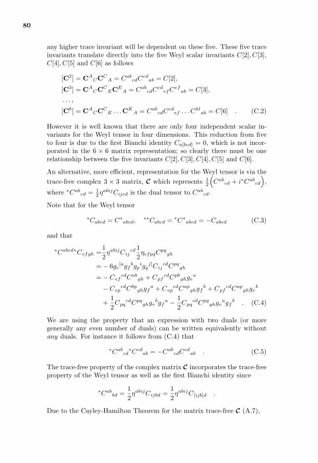
80
any higher trace invariant will be dependent on these five. These five traceinvariants translate directly into the five Weyl scalar invariants C[2], C[3],C[4], C[5] and C[6] as follows
[C2] = CACCC
A = CabcdC
cdab = C[2],
[C3] = CACCC
ECEA = Cab
cdCcd
efCefab = C[3],
. . . ,
[C6] = CACCC
E . . .CKA = Cab
cdCcd
ef . . . Cklab = C[6] . (C.2)
However it is well known that there are only four independent scalar in-variants for the Weyl tensor in four dimensions. This reduction from fiveto four is due to the first Bianchi identity Ca[bcd] = 0, which is not incor-porated in the 6 × 6 matrix representation; so clearly there must be onerelationship between the five invariants C[2], C[3], C[4], C[5] and C[6].
An alternative, more efficient, representation for the Weyl tensor is via thetrace-free complex 3 × 3 matrix, C which represents 1
2
(Cab
cd + i∗Cabcd
),
where ∗Cabcd = 1
2ηabijCijcd is the dual tensor to Cabcd.
Note that for the Weyl tensor
∗Cabcd = C∗abcd,∗∗Cabcd = ∗C∗abcd = −Cabcd (C.3)
and that
∗Cabcd∗Cefgh =12ηabijCij
cd 12ηefpqC
pqgh
=− 6ge[agf
bgpigq
j]CijcdCpq
gh
=− CefcdCab
gh + CpfcdCpb
ghgea
− CepcdCbp
ghgfa + Cep
cdCapghgf
b + CpfcdCap
ghgeb
+12Cpq
cdCpqghge
bgfa − 1
2Cpq
cdCpqghge
agfb . (C.4)
We are using the property that an expression with two duals (or moregenerally any even number of duals) can be written equivalently withoutany duals. For instance it follows from (C.4) that
∗Cabcd∗Ccd
ab = −CabcdC
cdab . (C.5)
The trace-free property of the complex matrix C incorporates the trace-freeproperty of the Weyl tensor as well as the first Bianchi identity since
∗Cabbd =
12ηabijCijbd =
12ηabijC [ijb]d .
Due to the Cayley-Hamilton Theorem for the matrix trace-free C (A.7),
August 20, 2004 (15:33)

81
coC3 + c2C + c3I = 0 ,
there are only two complex trace invariants of this complex three-dimen-sional trace-free matrix, I = [C2] and J = [C3], and so four real invariantsare obtained directly. (These two complex invariants also follow easily fromspinor considerations, as shown in Appendix A )
Clearly there must be simple direct relationships between I, J and C[2],C[3], C[4],C[5] and C[6], and just writing out I, J in terms of the Weyltensor and its dual we get
I =[C2] =14(Cab
cd + i∗Cabcd
)(Ccd
ab + i∗Ccdab
)
=12
(Cab
cdCcd
ab + iCabcd∗Ccd
ab
)(C.6)
and
J =[C3] =18(Cab
cd + i∗Cabcd
)(Ccd
ef + i∗Ccdef
)(Cef
ab + i∗Cefab
)
=12
(Cab
cdCcd
efCefab − i∗Cab
cd∗Ccd
ef∗Cef
ab
). (C.7)
We would now like to eliminate the duals in these expressions and we dothis by using (C.4). So, for the complex term in (C.6) we find,
(∗CabcdCcd
ab)2 =∗Cab
cdCcdab∗Cef
ghCghef
=− 2CabcdC
cdefCef
ghCghab − 4Cab
cdCefcdCafghCbe
gh
=− 2C[4]− 4CabcdC
efcdCafghCbegh . (C.8)
Since it is known that there are only four scalar invariants of the Weyltensor in four dimensions, the second term must be expressible in terms ofC[2], C[3], C[4], C[5], C[6]. Note that since this term is quartic in the Weyltensor it must be a linear combination of (C[2])2 and C[4]. To find thislinear combination
CabcdC
efcdCafghCbegh = α C[4] + β
(C[2]
)2
(C.9)
(α and β constants) we can use dimensionally dependent identities or wecan start by making the ansatz (C.9), calculate1 the expression for a fewmetrics, and thereby determine α and β.
Doing this we find
CabcdC
efcdCafghCbegh =
12
C[4]− 14
(C[2]
)2
(C.10)
1Here the computer tools are very useful, for example GRTensor II [18].
August 20, 2004 (15:33)

82
and hence we get from (C.8) that
(∗CabcdCcd
ab)2 = −4C[4] +
(C[2]
)2
. (C.11)
Using similar methods as described above we can find an expression for∗Cab
cd∗Ccd
ef∗Cef
ab in (C.7) in terms of C[2], C[3], C[4], C[5], C[6]
(∗Cabcd∗Ccd
ef ∗Cefab
)2 = −6C[6]+(C[3]
)2
+92C[2]C[4]−3
4
(C[2]
)3
(C.12)
and also
(∗Cabcd∗Ccd
ef ∗Cefab
)(∗CghijCij
gh)
=125
C[5]− C[2]C[3] . (C.13)
From (C.11), (C.12) and (C.13) we now find
I =[C2] =14(Cab
cd + i∗Cabcd
)(Ccd
ab + i∗Ccdab
)
=12
(Cab
cdCcd
ab + iCabcd∗Ccd
ab
)=
12
(C[2] + i
√−4C[4] +
(C[2]
)2)
(C.14)
and
J =[C3] =18(Cab
cd + i∗Cabcd
)(Ccd
ef + i∗Ccdef
)(Cef
ab + i∗Cefab
)
=12
(Cab
cdCcd
efCefab − i∗Cab
cd∗Ccd
ef∗Cef
ab
)
=12
(C[3]− i
√−6C[6] +
(C[3]
)2
+92C[2]C[4]− 3
4
(C[2]
)3)
. (C.15)
It follows directly that
II = −C[4] +12
(C[2]
)2
(C.16)
JJ = −32C[6] +
12
(C[3]
)2
+98C[2]C[4]− 3
16
(C[2]
)3
. (C.17)
Using
((∗Cabcd∗Ccd
ef ∗Cefab
)(∗CghijCij
gh))2
=(∗Cab
cdCcdab
)2(∗Cabcd∗Ccd
ef ∗Cefab
)2 (C.18)
August 20, 2004 (15:33)
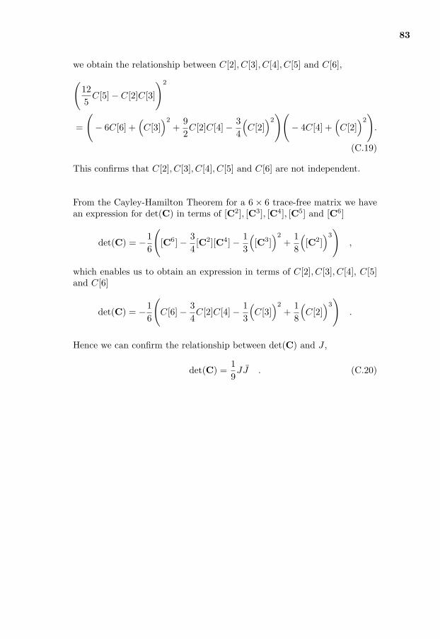
83
we obtain the relationship between C[2], C[3], C[4], C[5] and C[6],
(125
C[5]− C[2]C[3]
)2
=
(− 6C[6] +
(C[3]
)2
+92C[2]C[4]− 3
4
(C[2]
)2)(
− 4C[4] +(C[2]
)2)
.
(C.19)
This confirms that C[2], C[3], C[4], C[5] and C[6] are not independent.
From the Cayley-Hamilton Theorem for a 6× 6 trace-free matrix we havean expression for det(C) in terms of [C2], [C3], [C4], [C5] and [C6]
det(C) = −16
([C6]− 3
4[C2][C4]− 1
3
([C3]
)2
+18
([C2]
)3)
,
which enables us to obtain an expression in terms of C[2], C[3], C[4], C[5]and C[6]
det(C) = −16
(C[6]− 3
4C[2]C[4]− 1
3
(C[3]
)2
+18
(C[2]
)3)
.
Hence we can confirm the relationship between det(C) and J ,
det(C) =19JJ . (C.20)
August 20, 2004 (15:33)

Appendix D
Computer tools
In this thesis we have carried out some long calculations, often with expres-sions involving several hundreds of terms. To perform these calculationstwo software packages have proven particularly useful, GRTensor II andTensign. In this appendix we give a short introduction to each of them andhow they have been used.
D.1 GRTensor II
On http://grtensor.phy.queensu.ca/ or http://grtensor.org/ , where alsoGRTensor II can be downloaded free of charge, one can read:
“GRTensor II is a computer algebra package for performing calculationsin the general area of differential geometry. Its purpose is the calculationof tensor components on curved spacetimes specified in terms of a metricor set of basis vectors. The package contains a library of standard defini-tions of a large number of commonly used curvature tensors, as well as theNewman-Penrose formalism. The standard object libraries are easily ex-pandable by a facility for defining new tensors. Calculations can be carriedout in spaces of arbitrary dimension, and in multiple spacetimes simultane-ously. Though originally designed for use in the field of general relativity,GRTensorII is useful in many other fields. GRTensor II is not a stand alonepackage, but requires an algebraic engine. The program was originally de-veloped for MapleV.GRTensorII runs with all versions of Maple, Maple VRelease 3 to Maple 9.5. A limited version (GRTensorM) has been portedto Mathematica.”
In this thesis we have mainly used GRTensor II to prove negative resultsvia explicit counterexamples.
August 20, 2004 (15:33)

85
D.2 Tensign
Tensign is a program developed by Anders Hoglund for handling and ma-nipulating indices associated with tensor expressions. The program aidsthe user in keeping track of all details in calculations, such as coefficients,symmetries, signs, trace properties etc., and is an invaluable tool for sim-plifying, expanding and rewriting tensor expressions.
In Tensign one can define tensors with any kind of symmetries and ofarbitrary order. In addition, all other properties, e.g., relations to othertensors or trace properties, are defined by rules which can be applied toan expression or part of an expression. A defined rule can only be appliedto a specific type of tensor, making it impossible to make mistakes in thecalculations.
One of the strengths with Tensign is that the user has full control overthe calculation at all times, and all operations are, and have to be, made“by hand” − the program is not “smart” in the sense that it does anycalculations, simplifications or other operations by itself.
In this thesis Tensign was used to derive the identities in Appendix B andthe conformal calculations in Chapter 4
To learn more about Tensign, its interface, etc, see either [23] or visit thehomepage http://www.lysator.liu.se/˜andersh/tensign/ .
August 20, 2004 (15:33)

86
August 20, 2004 (15:33)
References
[1] R. Bach, Zur Weylschen Relativitatstheorie und der Weylschen Er-weiterung des Krummungstensorbegriffs, Math. Zeitschr. 9 (1921) 110-135
[2] A. Balfagon, X. Jaen, Review of some classical gravitational superen-ergy tensors using computational techniques, Class. Quantum Grav.17 (2000) 2491-2497
[3] R. J. Baston and L. J. Mason, Conformal gravity, the Einstein equa-tions and spaces of complex null geodesics, Class. Quantum Grav. 4(1987) 815-826
[4] R. J. Baston and L. J. Mason, The conformal Einstein equations, Fur-ther advances in twistor theory Vol II (L. J. Mason, L. P. Hughstonand P. Z. Kobak eds), Longman Scientific & Technical, 1995
[5] D. Bini, R. T. Jantzen and G Miniutti, The Cotton, Simon-Mars andCotton-York tensors in stationary spacetimes, Class. Quantum Grav.18 (2001) 4969-4981
[6] H. W. Brinkmann, Riemann spaces conformal to Einstein spaces,Math. Ann. 91 (1924) 269-278
[7] H. W. Brinkmann, Einstein spaces which are mapped conformally oneach other, Math. Ann. 94 (1924) 119-145
[8] A. Coley, R. Milson, V. Pravda and A. Pravdova, Classification of theWeyl tensor in higher dimensions, Class. Quantum Grav. 21 (2004)L35-L41
[9] A. Coley, R. Milson, V. Pravda and A. Pravdova, Aligned null di-rections and tensor classification, arXive preprint: gr-qc/0401010,http://www.arxiv.org
[10] A. Coley, R. Milson, V. Pravda and A. Pravdova, Bianchiidentities in higher dimensions, arXive preprint: gr-qc/0401013,http://www.arxiv.org
August 20, 2004 (15:33)
88
[11] C. D. Collinson, A class of conserved tensors in an arbitrary gravita-tional field, Proc- Cam. Phil. Soc. 58 (1962) 346-363
[12] S. R. Czapor, R. G. McLenaghan and V. Wunsch, Conformal C andEmpty Spaces of Petrov Type N, Gen. Rel. Grav., Vol. 34 (2002) 385-402
[13] S. B. Edgar, Necessary and sufficient conditions for n-dimensional con-formal Einstein spaces via dimensionally dependent identities, arXivepreprint: math.DG/0404238, http://www.arxiv.org
[14] S. B. Edgar and A. Hoglund, Dimensionally dependent tensor identi-ties by double antisymmetrization, J. Math. Phys. 43 (2002) 659-677
[15] A. A. Garcıa, F. W. Hehl, C. Heinicke and A. Macıas, The Cottontensor in Riemannian spacetimes, Class. Quantum Grav. 21 (2004)1099-1118
[16] A. R. Gover and P. Nurowski, Obstructions to conformally Ein-stein metrics in n dimensions, arXive preprint: math.DG/0405304,http://www.arxiv.org
[17] C. Gregory, Non-linear Invariants and the Problem of Motion, Phys.Rev. 72 (1947) 72-75
[18] GRTensorII, http://grtensor.phy.queensu.ca/ or http://grtensor.org/
[19] G. B. Gurevic, Foundations of the theorey of algebraic invariants, P.Noordhoff Ltd - Groningen, 1964
[20] J. Haantjes and J. A. Schouten, Betrage zur allgemeinen (gekrumten)konformen Differentialgeometrie I, II, Math. Ann. 112 (1936) 594-629;113 (1936) 568-583
[21] G. S. Hall and M. S. Capocci, Classification and conformal symmetryin three-dimensional space-times, J. Math. Phys. 40 (1999) 1466-1478
[22] B. Hesselbach, Uber die Erhaltungssatze der konformen Geometrie,Math. Nachr. 3 (1949) 107-126
[23] A. Hoglund, The Lanczos potential, dimensionally dependent identi-ties and algebraic Rainich theory, Tekn. D. dissertaion, Matematiskainstitutionen, Linkopings universitet, Linkoping, Sweden, 2002, ISBN91-7373-285-0
[24] I. Jach and L. Parker, Linear independence of renormalisation coun-terterms in curved space-times of arbitrary dimensionality, J. Math.Phys. 28 (1987) 1137-1139
August 20, 2004 (15:33)

89
[25] M. Korzynski and J. Lewandowski, The normal conformal Cartan con-nection and the Bach tensor, Class. Quantum Grav. 20 (2003) 3745-3764
[26] C. N. Kozameh, E. T. Newman and P. Nurowski, Conformal Einsteinequations and Cartan conformal connection, Class. Quantum Grav. 20(2003) 3029-3035
[27] C. N. Kozameh, E. T. Newman and K. P. Tod, Conformal EinsteinSpaces, Gen. Rel. and Grav., Vol. 17 (1985) 343-352
[28] M. Listing, Conformal Einstein Spaces in N-dimensions, Annals ofGlobal Analysis and Geometry, 20 (2001) 183-197
[29] D. Lovelock, Dimensional dependent identities, Proc. Cambridge Phi-los. Soc. 68 (1970) 345-350
[30] S. A. Merkulov, A conformally invariant theory of gravitation andelectromagnetism, Class. Quantum Grav. 1 (1984) 349-354
[31] P. Nurowski and J. F. Plebanski, Non-vacuum twisting type-N metrics,Class. Quantum Grav. 18 (2001) 341-351
[32] R. Penrose, W. Rindler, Spinors and space-time, vol. 1, CambridgeUniv. Press, 1984
[33] R. Penrose, W. Rindler, Spinors and space-time, vol. 2, CambridgeUniv. Press, 1986
[34] I. Robinson, On the Bel-Robinson tensor, Class. Quantum Grav. 14(1997) A331-A333
[35] R. K. Sachs, Propagation laws for null and type III gravitational waves,Z. Phys. 157 (1960) 462-477
[36] J. A. Schouten, Ricci-calculus, 2nd. ed. (1954) Springer-Verlag, Berlin
[37] J. A. Schouten, Uber die konforme Abbildung n-dimensionaler Man-nigfaltigkeiten mit quadratischer Massbestimmung auf eine Mannig-faltigkeit mit euklidischer Massbestimmung, Math. Zeitschr. 11 (1921)58-88
[38] G. E. Shilov, Linear algebra, Dover Publications Inc., 1977
[39] P. Szekeres, Spaces conformal to a class of spaces in general relativity,Proc. Roy. Soc. London, Ser. A 274 (1963) 206-212
[40] R. M. Wald, General Relativity, The University of Chicago Press, 1984
[41] H. Weyl, Reine Infinitesimalgeometrie, Math. Zeitschr. 2 (1918) 384-411
August 20, 2004 (15:33)

90
[42] O. Wingbrant, Highly structured tensor identities for (2, 2)-forms infour dimensions, arXive preprint: gr-cq/031120, http://www.arxiv.org
[43] V. Wunsch, C-Raume und Huygenssches Prinzip, Wiss. Zeitschr. Pad.Hochsch. Erfurt-Muhlhausen, Math.-Naturw. R 20 (1987) 103-111
[44] V. Wunsch, Conformal C- and Einstein Spaces, Math. Nachr. 146(1990) 237-245
August 20, 2004 (15:33)