European Journal of Mechanics B/Fluids 29 (2010) 369–376

Contents lists available at ScienceDirect

European Journal of Mechanics B/Fluids

journal homepage: www.elsevier.com/locate/ejmflu

Conformal contour dynamics in bounded domainsIrene Gned, Haysam Telib, Luca Zannetti ∗Politecnico di Torino, DIASP, Italy

a r t i c l e i n f o

Article history:Received 16 December 2009Received in revised form22 March 2010Accepted 1 April 2010Available online 24 April 2010

Keywords:Vortex patchesComplex analysisContour dynamics

a b s t r a c t

A contour dynamics algorithm is presented for vortex patches in unbounded domains and in simplyconnected bounded domains. It is based on conformal mapping and spectral analysis. The inside andoutside of a vortex patch are analytically mapped onto the inside and outside of the unit circles of twodifferent complex planes. The flow field is determined by matching the inner and outer flows on thepatch boundary. Following the Legras and Zeitlin conformal dynamics concept, the time evolution of thepatch boundary is expressed by means of the time derivatives of the mapping functions. The presenceof a bounding wall, which can be permeable and movable, is considered. The geometry and dynamicsof the patch and the flow velocity on the bounding wall are represented by Fourier series; by assumingtheir coefficients as control parameters, the proposed formulation can be appealing for optimization andcontrol purposes. Two numerical examples of the proposed technique are presented.

© 2010 Elsevier Masson SAS. All rights reserved.

1. Introduction

This study is part of an effort devoted to the development oftools for the control of the unsteady wake past bluff bodies orof the massively separated flow past obstacles protruding from awall. The goal is to reduce flow unsteadiness which is responsiblefor undesirable flow characteristics such as high drag, noise,vibrations.Flow unsteadiness is generally caused by the shedding of large-

scale coherent rotational structures which can be modeled inseveral ways. The simplest approach to study a control strategy forreducing the phenomenon uses point vortices tomodel the vorticalstructures. Cortelezzi’s [1] feedback control of the wake past anorthogonal flat plate was based on this model. It has also beenused for passive control of a wake in [2] and for optimal control,by blowing and suction, of a vortex trapped by a cavity in [3].An approach that is more consistent with real world applica-

tionsmodels the vortical structures as rotational regions with con-stant vorticity, that is, as vortex patches. Indeed, Batchelor’s flowmodel [4] is physically consistent to represent a high Reynoldsnumber steady recirculating flow. In [5] it is shown how the steadywake past a circular cylinder can be modeled by different vortexpatches embedded in a potential flow. The study of the existence,in general, of such steady solutions has been carried out in [6].The contour dynamics algorithm, as devised by Zabusky et al.

[7] (see also [8]), is a simple and fast numerical tool for the study

∗ Corresponding author.E-mail addresses: irene.gned@polito.it (I. Gned), haysam.telib@polito.it

(H. Telib), luca.zannetti@polito.it (L. Zannetti).

0997-7546/$ – see front matter© 2010 Elsevier Masson SAS. All rights reserved.doi:10.1016/j.euromechflu.2010.04.001

of the dynamics of vortex patches in unbounded domains. Briefly,according to the Green function approach, the entire velocity field,for a given vorticity ω, depends only on the shape of the patchboundary and can be determined by a line integral along it. Thus,the geometry of the patch can be updated by integrating theboundary velocity in time and, as a consequence, the dynamics ofthe entire flow field can be determined in time.Unfortunately the extension of the algorithm to general multi-

connected bounded domains is not straightforward. Only recentlyhave Crowdy and Surana [9] provided a general formulationfor a contour dynamics algorithm for multi-connected domainsbounded by arbitrary impermeable boundaries. Their approachis based on the Green function which defines the Hamiltonianof point vortices in bounded domains, and on its transformationunder conformal mapping, as devised by Masotti [10] forsimply connected domains and generalized to multiply connecteddomains by Lin [11].As discussed in [9], previous extensions of the contour

dynamicsmethodwere limited in practice to the case of straight orcircular impermeable boundaries (see, for instance, the examplesworked out in [12–14]).An alternative formulation of the problem of determining the

dynamics of a vortex patch in an unbounded domain exploits theSchwarz function concept. It is described in Section 9.2 of Ref. [8]and the references therein.A further method is proposed in the present work, which

does not explicitly use the Schwarz function concept, but can beconsidered as inspired by it. Formulations for unbounded domainsas well as for domains bounded by a single, arbitrarily shaped wallare provided here. A novel feature of the proposed method is thatthe bounding wall can be considered as movable. From a different

370 I. Gned et al. / European Journal of Mechanics B/Fluids 29 (2010) 369–376

z-planeλ-plane ζ-plane

De

Fig. 1. Physical unbounded domain and transformed planes.

viewpoint this feature also allows the imposition of a permeabilitycondition (as needed for modeling blowing and suction). In fact,the parameters that define the behavior of the control devices,such as bounding wall motion or blowing and suction, appear ascoefficients in a spectral formulation. Furthermore, the parameterswhich define the shape of the patch and its rate of deformationalso appear as coefficients in the formulation. They can be usedas explicit control parameters for the optimal manipulation of thepatch (e.g. in order to find the equilibrium configuration) and/orfor operating the control devices.Hence, in addition to the general interest in enlarging the

panorama of vortex dynamics methods, the present formulationprovides a framework for the dual problems of optimization andcontrol by a movable wall or a permeability condition. The controlproblem however is seen in perspective and it is not treated hereas the main focus of the paper is the description of the proposedpatch dynamics algorithm. Finally, the proposed method gainssome computational efficiency by exploiting the idea of conformalmap dynamics of Legras and Zeitlin [15].The presentmethod shares with the Schwarz function formula-

tion the drawback of being unable to follow the contour evolutionwhen it becomes too far from a more or less rounded shape andfilamentation phenomena occur. Nevertheless the class of geome-tries which can be studied is reasonably large, that is sufficientlylarge for one to be able to address optimization and control prob-lems.The paper is organized as follows: in Section 2 the proposed for-

mulation is described for unbounded domains and its relationshipwith the Schwarz function approach is discussed. In Section 2.5 themethod is checked by using as a benchmark, in a non-trivial form,the Kirchhoff’s analytical solution for elliptical vortex patches. InSection 3 the formulation is extended to bounded simply con-nected domains with movable and/or permeable walls. The ap-proach for bounded domains with blowing and suction is checkedversus an analytical solution in Section 3.3. Concluding remarks aredrawn in Section 4.

2. Vortex patches in unbounded domains

We consider the unbounded 2Dmotion of an inviscid fluid tak-ing place on the complex z-plane (z = x + iy). Let Di be a simplyconnected vortex patch, with vorticityω and bounded by ∂ , and letDe be the irrotational region which is external to it and extends toinfinity. As shown in Fig. 1, the regionDi is conformallymapped in-side the unit circle of the transformed ζ -plane and the region De ismapped outside the unit circle of the transformedλ-plane. Accord-ing to the Riemann mapping theorem such mappings exist, theycan be expressed as Theodorsen–Garrick [16,17] transformations,that is, Di is mapped inside the unit circle of the ζ -plane by

z(ζ )− zo = ζ exp∞∑n=0

anζ n (1)

and De is mapped outside the unit circle of the λ-plane by

z(λ)− zo = λ exp∞∑n=0

bnλ−n (2)

where zo is a point inside the patch. Once the series are truncatedat a sufficiently large value n = N , the coefficients an and bn canconveniently be determined according to the iterative process pro-posed by Ives [17].In De the motion is irrotational and a complex potential we can

be defined. For regularity reasons, the complex velocity dwe/dz hasto be a holomorphic function of z in De. Since z(λ) (defined by (2))is holomorphic outside the unit circle of the λ-plane, the complexvelocity can, in general, be expressed by the series

ue − ive =dwedz=

∞∑j=0

cjλ−j. (3)

In Di the motion has constant vorticity ω and the complex velocitycan in general be expressed as ui − ivi = −iω/2z? + dwi/dz, withdwi/dz analytic and holomorphic in Di and with (?) denoting thecomplex conjugate. For the same regularity reason as above, it fol-lows that the inner complex velocity can, in general, be expressedas a function of ζ by

ui − ivi = −iω

2[z(ζ )]? +

∞∑j=0

djζ j. (4)

Let ζ = ρi exp(iϕi) and λ = ρe exp(iϕe). According to the map-pings (1), (2) each patch contour point z∂ is the image of a point ofthe unit circle of the ζ -plane and of a point of the unit circle of theλ-plane, that is,

z∂ − zo = exp

[iϕ∂ i +

N−1∑n=0

an exp(inϕ∂ i)

]

= exp

[iϕ∂e +

N−1∑n=0

bn exp(−inϕ∂e)

](5)

which establishes an implicit relationship F(ϕ∂ i, ϕ∂e) = 0 amongthe anomalies of the two unit circles. In principle, by making ex-plicit ϕ∂ i or ϕ∂e, the relationship ϕ∂ i = ϕ∂ i(ϕ∂e) and its inverseϕ∂e = ϕ∂e(ϕ∂ i) can be found.By equating the internal and external flow velocities at the

patch contour, Eqs. (3) and (4), truncated at a large value j = J ,yield

J−1∑j=0

cj exp(−ijϕ∂e) = −iω

2[z(ϕ∂ i(ϕ∂e))]?

+

J−1∑j=0

dj exp[ijϕ∂ i(ϕ∂e)] (6)

and

− iω

2[z(ϕ∂ i)]? +

J−1∑j=0

dj exp[i jϕ∂ i] =J−1∑j=0

cj exp(−ijϕ∂e(ϕ∂ i)) (7)

each one ofwhich should allow the coefficients cj and dj, that is, theflow velocity, to be determined. The patch geometry could then beupdated by letting its boundary be drifted by the flow.

I. Gned et al. / European Journal of Mechanics B/Fluids 29 (2010) 369–376 371

2.1. The functions ϕ∂ i(ϕ∂e) and ϕ∂e(ϕ∂ i)

The above idea has been implemented here in a practical wayfor vortex patches belonging to the so-called star-shaped class. Letϑ∂ = arg(z∂ − zo). The patch is said to be star-shaped if thereexists zo such that r∂ = |z∂ − zo| is a single valued function of ϑ∂ .Not incidentally, such a class coincides with the class of shapes forwhich the Theodorsen–Garrickmappings (1) and (2) can be carriedout.The function ϕ∂ i(ϕ∂e) and its inverse ϕ∂e(ϕ∂ i) are determined by

means of a numerical procedure based on periodic splines. Fromlog(z∂ − zo) = log r∂ + iϑ∂ and from Eq. (1), one gets

ϑ∂(ϕ∂ i) = ϕ∂ i + Im

[N−1∑n=0

an exp(inϕ∂ i)

]. (8)

Let δ = ϕ∂ i − ϑ∂(ϕ∂ i). A vector of values (ϑ∂(ϕ∂ i), δ) can be builtfor a discrete set of values of ϕ∂ i and a continuous representationδ = δ(ϑ∂) can be obtained by a periodic (cubic) spline. FromEq. (2)one gets

ϑ∂(ϕ∂e) = ϕ∂e + Im

[N−1∑n=0

bn exp(−inϕ∂e)

]. (9)

and the function ϕ∂ i(ϕ∂e) is given by

ϕ∂ i = δ(ϑ∂(ϕ∂e))+ ϑ∂(ϕ∂e). (10)

The same procedure is followed by inverting the role of Eqs. (9)and (10) to get the inverse function ϕ∂e(ϕ∂ i).Since the method is restricted to star-shaped patches, it fails

if filamentation phenomena occur. This is a consequence ofthe adopted Theodorsen–Garrick mapping and of the numeri-cal method used to obtain the matching functions ϕ∂ i(ϕ∂e) andϕ∂e(ϕ∂ i), which require that the functions ϑ∂(ϕ∂e) and ϑ∂(ϕ∂ i) bestrictly monotonic. This drawback is not absolute and could beovercome by struggling with conformal mapping. For instance,any non-star-shaped domain could be first mapped onto a star-shaped one by an appropriate pre-mapping transformation andthen mapped onto a circle as above. The functions ϕ∂ i(ϕ∂e) andϕ∂e(ϕ∂ i) could then be obtained by exploiting the implicit relation-ship z∂(ϕ∂e) = z∂(ϕ∂ i) between the physical and the transformedplanes. The real difficulty lies in the pre-mapping, which requiresad hoc functions and hence may not be included in an automaticprocess.

2.2. The flow velocity

Once the coefficients cj and dj on the right-hand sides ofEqs. (3) and (4) are computed, the flow velocity inside and outsidethe patch is determined. The coefficients cj and dj are numericallycomputed by means of a fixed point iterative process based on thecondition that the inner and outer flow velocities, as expressed byEqs. (7) and (8), have to match on the contour. Setting cj = crj+ icijand dj = drj + idij, the imaginary part of Eq. (7) yields

J−1∑j=0

[cij cos(jϕ∂e)− crj sin(jϕ∂e)]

=

J−1∑j=0

[dij cos(jϕ∂ i(ϕ∂e))+ drj sin(jϕ∂ i(ϕ∂e))]

−ω

2Im[iz?∂ (ϕ∂e)] (11)

and the real part of Eq. (8) yieldsJ−1∑j=0

[drj cos(jϕ∂ i)− dij sin(jϕ∂ i)]

=

J−1∑j=0

[crj cos(jϕ∂e(ϕ∂ i))+ cij sin(jϕ∂e(ϕ∂ i))]

+ω

2Re[iz?∂ (ϕ∂ i)]. (12)

An initial set of J values are guessed for dj (typically, dj = 0). Bydividing the unit circle of the λ-plane into 2J equispaced intervals,the right-hand side of Eq. (11) can be evaluated for 2J values ofϕ∂e and the FFT algorithm can be used to compute J values of cj.Dividing the unit circle of the ζ -plane into 2J equispaced intervals,the right-hand side of Eq. (12) can be evaluated for 2J values ofϕ∂ i and the FFT algorithm provides a new set of J values of dj.The process is repeated until, in a prescribed range, convergenceis achieved.It has to be noted that Eq. (11) does not provide cr0 and Eq. (12)

does not provide di0. Their values are defined by the value of thecomplex velocity q∞ at infinity in the physical plane. According toEq. (3) cr0 + ici0 = q∞; it follows that cr0 = Re(q∞) and that di0has to be such that ci0 = Im(q∞). By enforcing Eq. (11) for ϕ∂ i = 0,it follows that

di0 = −J−1∑j=1

dij + Im(q∞)

+

{J−1∑j=1

[cij cos(jϕ∂e)− crj sin(jϕ∂e)] +ω

2Im[iz?∂ ]

}ϕ∂ i=0

.

2.3. The contour evolution as conformal dynamics

As a consequence of the material nature of a vortex patch, theevolution in time of its contour coincides with its advection. Inprinciple this can be carried out by numerically integrating itsvelocity dz∂/dt in time. Such a procedure is neither convenientnor simple; actually, at each time step the updated geometryshould undergo the entire process explained above, including thelaborious and time consuming Ives [17] iterative computation ofthe new set of coefficients an and bn of the mappings (1) and (2).Following the ideas proposed by Legras and Zeitlin [15], a more

robust and faster procedure can be implemented which avoids theiterative process by computing, in closed form, the time derivativesan and bn of the mapping coefficients. These are integrated in timeand the updated shape of the patch is then obtained as the newmap of the unit circle of both the ζ and λ-plane.Let us first take into consideration the mapping (2). The

coordinate zp of a fluid particle depends on time through itstransformed coordinate λ and through the time-dependence of thecoefficients bn. The Lagrangian derivative of log(zp) is then

1zp

dzpdt= h(λ)

λ

λ+

N−1∑n=0

bnλ−n (13)

with h(λ) = 1 −∑N−1n=1 n bnλ

−n. For the points on the contour(|λ| = 1) one has Re(λ/λ) = 0, thus

Re

[1h(λ)

N−1∑n=0

bnλ−n]|λ|=1

= Re[(ue − ive)?

(z∂ − zo)h(λ)

]|λ|=1

,

with z∂ and (ue − ive) given by Eqs. (2) and (4), respectively. Theleft-hand side is the real part of a function of λ which is holo-morphic outside the unit circle. Let us call such a function H(λ).

372 I. Gned et al. / European Journal of Mechanics B/Fluids 29 (2010) 369–376

The definition of its imaginary part, once its real part is known onthe unit circle, is a classical problem which can be accomplishedin several manners. In the general spirit of the numerical proce-dures here adopted, we solve the problem by expressing H(λ) asH(λ) =

∑N−1n=0 enλ

−n and by computing the coefficients en bymeans of the FFT algorithm applied to its known real part. OnceH(λ) is determined, one can compute

∑N−1n=0 bnλ

−n= h(λ)H(λ)

and, finally, the coefficients bn can be found by applying the FFT al-gorithm again to either the real or the imaginary part of the right-hand side as evaluated on the unit circle.The procedure for computing the derivatives an of the

coefficients of the internalmapping (1) follows the same guideline,with the trivial variation that the unknown functions to bedetermined are holomorphic inside instead of outside the unitcircle.

2.4. The relationship with the Schwarz function method

The present method is similar to the Schwarz function method,as described, for instance, in [8]. In that method, the Eqs. (3) and(4) are replaced by functions of the physical complex coordinatez: ue − ive = −iω/2G(z) and ui − ivi = iω/2[F(z)− z?]with

G(z) =∞∑j=1

gnz−n, F(z) =∞∑j=0

fnzn

and where Φ(z) = F(z)+ G(z) results as the Schwarz function ofthe patch contour, expressed as a Laurent series converging in anannulus containing the contour. As in the present procedure, themethod then consists in determining the series coefficients. Withthe present method, the two parts of the Schwarz function, splitas shown above, are expressed in two different parametrizations,one outside the unit circle of the λ-parameter-plane and the otherone inside the unit circle of the ζ -parameter-plane. An advantageis that the solution is determined on the entire flow field and isnot limited to an annulus. Moreover, the class of possible contourgeometries which are contained in an annulus where the Laurentexpansion of their Schwarz functions converges is, quite reason-ably, smaller then the class of star-shaped contours for which thepresent method can be carried out. Finally, as shown below, thepresent formulation can be extended to domains confined by per-meable and movable walls.

2.5. A numerical example

The above method is tested by computing the motion of anelliptical vortex patch, as shown in Fig. 2, and by comparing theresult with the analytical Kirchhoff’s solution.Let lref =

√a2 − b2 and tref = 1/|ω| be the reference length

and the reference time respectively, with a and b being the ellipsesemiaxes. The simulation refers to an ellipsewith a = 5/4, b = 3/4and with a positive vorticity ω > 0. The ellipse center is displacedfrom the origin of the z-plane and, with reference to the mappings(1) and (2), zo is set equal to 0. As a consequence, the harmoniccontents of themapping series is enriched and the test is artificiallymade more severe than what would result for an ellipse centeredat the origin.The numbersN and J of the series coefficients are set toN = J =

50 and a second order Runge–Kutta algorithm is used to integratethe values of themapping coefficients in time. The integration timestep dt = .001 is selected by empirically verifying the stability ofthe integration process. Three frameshots relevant to a transientlasting for the non-dimensional time tend = 10, which correspondsto 10000 time steps, are shown in Fig. 2.At each time step, the patch boundary is computed twice, once

as the z∂e values of the external mapping, and once as the z∂ i values

Fig. 2. Simulation of the motion of an elliptical vortex patch.

-2.5

-3

-3.5

-4

-4.5

-5

-5.5

2000 4000 6000 8000 10000

Log(e1)

Log(e2)

-2

-6

para

met

riza

tion

s

Fig. 3. Evolution of Log(e1) and Log(e2) versus the integration time steps k.

of the internalmapping. The twogeometries are explicitly linked toeach other only by the common initial condition. Due to truncationerrors, they can diverge in time. Fig. 3 shows the behavior ofLog(e1) in time, with e1 being the L2 distance between the twosolutions. The same figure also shows the behavior of Log(e2) intime, where e2 is the L2 distance from the boundary, computedby the external mapping, to the analytical solution. Both of themappear to be almost constant in time. Their initial non-zero valueis a result of the interpolation needed to compare values computedon non-coincident collocation points.The small, but growing, oscillations shown by e2 at the end of

the time interval are due to the appearance of spurious high wavenumber oscillations of the patch boundary. They suggest that, for alonger integration time, the computation will eventually diverge.Such an event can be avoided by restarting the entire process byassuming the properly filtered final computed shape as the newinitial condition.

3. Confined domain

Let the flow region be a 2D simply connected domain boundedby a wall which can be a closed line or a line which extends to

I. Gned et al. / European Journal of Mechanics B/Fluids 29 (2010) 369–376 373

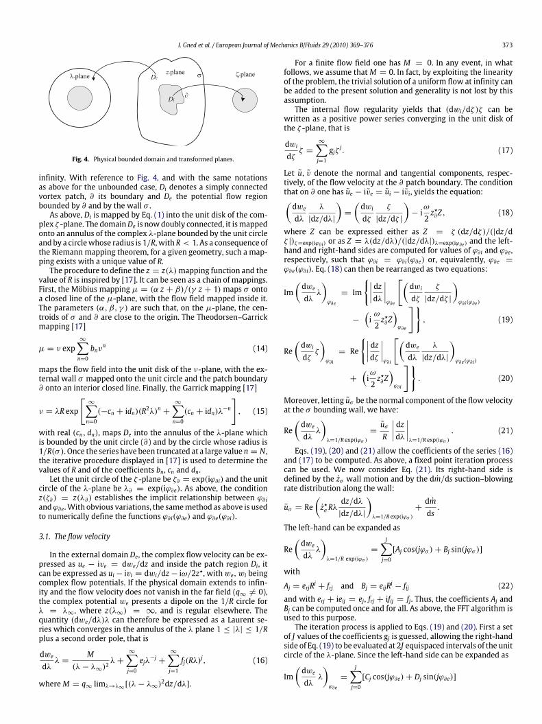
Fig. 4. Physical bounded domain and transformed planes.

infinity. With reference to Fig. 4, and with the same notationsas above for the unbounded case, Di denotes a simply connectedvortex patch, ∂ its boundary and De the potential flow regionbounded by ∂ and by the wall σ .As above, Di is mapped by Eq. (1) into the unit disk of the com-

plex ζ -plane. The domainDe is nowdoubly connected, it ismappedonto an annulus of the complex λ-plane bounded by the unit circleand by a circlewhose radius is 1/R, with R < 1. As a consequence ofthe Riemann mapping theorem, for a given geometry, such a map-ping exists with a unique value of R.The procedure to define the z = z(λ)mapping function and the

value of R is inspired by [17]. It can be seen as a chain of mappings.First, the Möbius mapping µ = (α z + β)/(γ z + 1)maps σ ontoa closed line of the µ-plane, with the flow field mapped inside it.The parameters (α, β, γ ) are such that, on the µ-plane, the cen-troids of σ and ∂ are close to the origin. The Theodorsen–Garrickmapping [17]

µ = ν exp∞∑n=0

bnνn (14)

maps the flow field into the unit disk of the ν-plane, with the ex-ternal wall σ mapped onto the unit circle and the patch boundary∂ onto an interior closed line. Finally, the Garrick mapping [17]

ν = λR exp

[∞∑n=0

(−cn + idn)(R2λ)n +∞∑n=0

(cn + idn)λ−n], (15)

with real (cn, dn), maps De into the annulus of the λ-plane whichis bounded by the unit circle (∂) and by the circle whose radius is1/R(σ ). Once the series have been truncated at a large value n = N ,the iterative procedure displayed in [17] is used to determine thevalues of R and of the coefficients bn, cn and dn.Let the unit circle of the ζ -plane be ζ∂ = exp(iϕ∂ i) and the unit

circle of the λ-plane be λ∂ = exp(iϕ∂e). As above, the conditionz(ζ∂) = z(λ∂) establishes the implicit relationship between ϕ∂ iandϕ∂e.With obvious variations, the samemethod as above is usedto numerically define the functions ϕ∂ i(ϕ∂e) and ϕ∂e(ϕ∂ i).

3.1. The flow velocity

In the external domain De, the complex flow velocity can be ex-pressed as ue − ive = dwe/dz and inside the patch region Di, itcan be expressed as ui− ivi = dwi/dz− iω/2z?, withwe, wi beingcomplex flow potentials. If the physical domain extends to infin-ity and the flow velocity does not vanish in the far field (q∞ 6= 0),the complex potential we presents a dipole on the 1/R circle forλ = λ∞, where z(λ∞) = ∞, and is regular elsewhere. Thequantity (dwe/dλ)λ can therefore be expressed as a Laurent se-ries which converges in the annulus of the λ plane 1 ≤ |λ| ≤ 1/Rplus a second order pole, that is

dwedλ

λ =M

(λ− λ∞)2λ+

∞∑j=0

ejλ−j +∞∑j=1

fj(Rλ)j, (16)

whereM = q∞ limλ→λ∞ [(λ− λ∞)2dz/dλ].

For a finite flow field one has M = 0. In any event, in whatfollows, we assume thatM = 0. In fact, by exploiting the linearityof the problem, the trivial solution of a uniform flow at infinity canbe added to the present solution and generality is not lost by thisassumption.The internal flow regularity yields that (dwi/dζ )ζ can be

written as a positive power series converging in the unit disk ofthe ζ -plane, that is

dwidζζ =

∞∑j=1

gjζ j. (17)

Let u, v denote the normal and tangential components, respec-tively, of the flow velocity at the ∂ patch boundary. The conditionthat on ∂ one has ue − ive = ui − ivi, yields the equation:(dwedλ

λ

|dz/dλ|

)=

(dwidζ

ζ

|dz/dζ |

)− iω

2z?∂Z, (18)

where Z can be expressed either as Z = ζ (dz/dζ )/(|dz/dζ |)ζ=exp(iϕ∂ i) or as Z = λ(dz/dλ)/(|dz/dλ|)λ=exp(iϕ∂e) and the left-hand and right-hand sides are computed for values of ϕ∂ i and ϕ∂e,respectively, such that ϕ∂ i = ϕ∂ i(ϕ∂e) or, equivalently, ϕ∂e =ϕ∂e(ϕ∂ i). Eq. (18) can then be rearranged as two equations:

Im(dwedλ

λ

)ϕ∂e

= Im

{∣∣∣∣ dzdλ∣∣∣∣ϕ∂e

[(dwidζ

ζ

|dz/dζ |

)ϕ∂ i(ϕ∂e)

−

(iω

2z?∂Z)ϕ∂e

]}, (19)

Re(dwidζζ

)ϕ∂ i

= Re

{∣∣∣∣ dzdζ∣∣∣∣ϕ∂ i

[(dwedλ

λ

|dz/dλ|

)ϕ∂e(ϕ∂ i)

+

(iω

2z?∂Z)ϕ∂ i

]}. (20)

Moreover, letting uσ be the normal component of the flow velocityat the σ bounding wall, we have:

Re(dwedλ

λ

)λ=1/R exp(iϕσ )

=uσR

∣∣∣∣ dzdλ∣∣∣∣λ=1/R exp(iϕσ )

. (21)

Eqs. (19), (20) and (21) allow the coefficients of the series (16)and (17) to be computed. As above, a fixed point iteration processcan be used. We now consider Eq. (21). Its right-hand side isdefined by the zσ wall motion and by the dm/ds suction–blowingrate distribution along the wall:

uσ = Re(z?σRλ

dz/dλ|dz/dλ|

)λ=1/R exp(iϕσ )

+dmds.

The left-hand can be expanded as

Re(dwedλ

λ

)λ=1/R exp(iϕσ )

=

J∑j=0

[Aj cos(jϕσ )+ Bj sin(jϕσ )]

with

Aj = erjRj + frj and Bj = eijRj − fij (22)

and with erj + ieij = ej, frj + ifij = fj. Thus, the coefficients Aj andBj can be computed once and for all. As above, the FFT algorithm isused to this purpose.The iteration process is applied to Eqs. (19) and (20). First a set

of J values of the coefficients gj is guessed, allowing the right-handside of Eq. (19) to be evaluated at 2J equispaced intervals of the unitcircle of the λ-plane. Since the left-hand side can be expanded as

Im(dwedλ

λ

)ϕ∂e

=

J∑j=0

[Cj cos(jϕ∂e)+ Dj sin(jϕ∂e)]

374 I. Gned et al. / European Journal of Mechanics B/Fluids 29 (2010) 369–376

with

Cj = eij + fijRj and Dj = −erj + frjRj,

J values of Cj andDj can be computed by the FFT algorithmand fromEq. (22) a set of values of ej, fj can be determined. It is then possibleto evaluate the right-hand side of Eq. (20). Since we have

Re(dwidζζ

)ϕ∂ i

=

J∑j=0

Re[gj exp(ijϕ∂ i)],

a new set of J values of the gj coefficients can be computed by theFFT algorithm and the process can be repeated until convergenceis achieved.

3.2. The wall and patch time evolution

Let the wall σ move and, as above, let zσ denote its velocity.Moreover, let it be understood that the mapping z = z(µ) coeffi-cients do not depend on time, then, on the µ-plane, the µσ imageof the wall will deform with the velocity µσ = zσ (dµ/dz)σ . Themapping (14) then yields

µσ

µσ= h(νσ )

νσ

νσ+

N−1∑n=0

bnνnσ

with h(νσ ) = 1 +∑N−1n=1 n bnν

nσ , which has the same structure as

Eq. (13). Since Re(νσ /νσ ) is equal to 0, the sameprocedure as abovecan be used to compute the timederivatives bn of the coefficients ofthe mapping (14). Should the mapping z = z(µ) depend on time,the variations of the procedure are obvious.The evolution of the patch boundary, seen as the evolution of

the coefficients of the mapping onto the ζ -plane, is not differentfrom the unbounded case treated above.Also the time derivatives cn, dn, R of the coefficients and of the

parameter R of the external mapping (15) can be determined inclosed form from the knowledge of the velocity of deformationof the patch and of the external boundary. As explained in detailbelow, a method inspired by that of Legras–Zeitlin [15] is adoptedfor this purpose.Let ν and λdenote the Lagrangian derivatives of amaterial point

as seen on the ν- and λ-planes, respectively. By taking the totalderivative of Eq. (15), it follows that the relationship between themis

ν

ν= h0(λ)

λ

λ+ h1(λ)

RR+ h2(λ) (23)

with

h0(λ) = 1+N−1∑n=1

n(−cn + idn)(R2λ)n −N−1∑n=1

n(cn + idn)λ−n

h1(λ) =

[1+

N−1∑n=1

2n(−cn + idn)(R2λ)n]

h2(λ) =N−1∑n=0

(−cn + idn)(R2λ)n +N−1∑n=0

(cn + idn)λ−n. (24)

Letting

g(λ) =h1(λ)R/R+ h2(λ)

h0(λ), (25)

Eq. (23) becomes

1h0(λ)

ν

ν=λ

λ+ g(λ). (26)

Since g(λ) has to be holomorphic inside the annulus of theλ-plane,it can be written as the Laurent series:

g(λ) =∞∑n=0

(en + ifn)(R2λ)n +∞∑n=0

(pn + iqn)λ−n.

We first consider the real part of Eq. (26) when applying it topoints belonging to the external wall σ :

Re[

1h0(λσ )

νσ

νσ

]= Re

[λσ

λσ

]+

N−1∑n=0

[En cos(nϕσ )+ Fn sin(nϕσ )]

with νσ = [r exp(iϑσ )]r=1, λσ = [ρ exp(iϕσ )]ρ=1/R, En = (en +pn)Rn and Fn = (qn − fn)Rn. For a point which moves arbitrarilywhile remaining attached to the wall, we have Re(νσ /νσ ) = 0,and Re[λσ /λσ ] = −R/R. Moreover, since Im[h0(λσ )] = 0, the left-hand side is null, implying that

E0 =RR, En = Fn = 0, (n = 1, 2, 3 . . .). (27)

Now let the real part of Eq. (26) be written for a fluid particle onthe ∂ patch boundary; since Re(λ∂/λ∂) = 0, the result is:

Re[1

h0(λ∂)ν∂

ν∂

]=

N−1∑n=0

[Pn cos(nϕ∂e)+ Qn sin(nϕ∂e)], (28)

with Pn = enR2n + pn and Qn = −fnR2n + qn. The quantity ν∂ canbe deduced from its relationship with the flow complex velocity:

z =[dwedλ

/dzdλ

]?=dzdµ

[∂µ

∂νν + ∂tµ

]where ∂tµ = µ

∑N−1n=0 bnν

n is the time derivative of the mapping(14). The left-hand side of Eq. (28) can thus be computed in 2Nequispaced points of the unit circle of the λ-plane, allowing Nvalues of the coefficients Pn,Qn to be computed by means of theFFT analysis.According to Eq. (27), the value of P0 = E0 = R/R provides

the value of R and the values of Pn and Qn define the values ofen = −pn, fn = qn (n = 1, 2, 3 . . .). As a consequence, g(λ) isknown and from Eq. (25) one gets

h2(λ) = g(λ) h0(λ)− h1(λ)RR

which allows h2(λ) to be computed on 2N equispaced points of theunit circle of the λ-plane. Finally, from Eq. (24), the FFT analysisof either its real or imaginary part defines N values of the timederivatives cn, dn of the coefficients of the mapping (15).

3.3. Numerical evaluation of the flow in a bounded domain

As far as we know, non-trivial, meaningful, exact solutions forvortex patches moving in a bounded domain can hardly be found.For instance, Crowdy [18] and Johnson & McDonald [19] haveprovided analytic solutions pertinent to rotational flows attachedto a solid body and smoothly confined by an external quiescentfluid. Unfortunately, these solutions refer to topologically differentflows and are unsuitable to be taken as benchmarks for the presentformulation.In order to test the accuracy of the method for predicting the

flow field and boundary velocity, we devised a test case, with wallblowing and suction, for which an analytical solution can be set up.We consider a circular vortex patch located inside an arbitrarily

shaped closed domain, as shown in Fig. 5. When the boundingwall is considered as solid and impermeable, the resulting flowis unsteady, with a non-null normal flow velocity at the patchboundary. This can be deduced by the instantaneous streamline

I. Gned et al. / European Journal of Mechanics B/Fluids 29 (2010) 369–376 375

Fig. 5. Left: instantaneous streamlines without blowing/suction. Right: steadystreamlines with blowing/suction.

pattern as computed by the above method and shown on the left-hand side of the same figure.We now apply blowing/suction to thebounding wall in order to manipulate the patch deformation. Forthe rate of blowing/suction uσ we choose the normal componentof the flow velocity that a Rankine vortex patch would induce onan unbounded domain at the wall points, that is

uσ = Re[ωr202i

Rλz(λ)− z0

dz/dλ|dz/dλ|

]λσ

,

where z0 is the circular patch center, r0 is the patch radius andz(λ) is the mapping function from the physical z-plane onto thetransformed λ-plane.With arguments related to the unicity of the solution, it can

easily be shown that the Rankine vortex flow is the solutionof the problem for the unbounded domain as well as for thebounded domain when such a blowing/suction rate is applied.Indeed, the above numerical method accurately approximates thissolution, as shown on the right-hand side of Fig. 5; where thecomputed streamline pattern is circular and the flow is steady. Thedistribution uσ pertinent to the adopted boundingwall is shown inFig. 6 as a function of the angular coordinate ϕ of the λ-plane. Therelative error on the flow velocity in the flow field is O(10−6), andthe error on the time derivatives an, bn of themapping coefficients,computed with N = J = 50, is of the same order of magnitude.It has to be noted that the assumption of a circular patch does

not make the problem trivial. In fact, on the ν-plane the image ofthe patch is no longer circular and the problem presents the samecomplexity as it would for an arbitrarily shaped patch.In general, there is no guaranty that the problem is well-posed.

An exhaustive discussion, about the ill-posedness of the controlproblem and about the methods to overcome it, goes beyond thepresent study. Here, we briefly address the point and allude topossible remedies.The above example refers to the problem of holding a vortex

patch of given geometry in equilibrium by wall blowing and suc-tion. Once the patch is assumed at rest, the inner solution of thePoissonproblem∇2ψ = −ω is uniquely determinedby theDirich-let condition ψ = const on the patch boundary. The external po-tential flow is then uniquely defined by the analytic continuationof the flow velocity from the patch boundary onto the external re-gion. As in the above example, the blowing/suction rate is definedby the normal component of the continued velocity on the outerwall. In general the problem is ill-posed because, depending on thepatch shape, the continuation can present singularities that, if lo-cated inside the external boundary, do not allow the existence of aholomorphic solution for the external flow field.Such ill-posedness can be eluded by weakening the problem.

Instead of seeking the blowing/suction rate needed to hold thepatch in a steady motion, we look for the rate which minimizes itsvelocity of deformation, that is, in a variational approach, the ratewhich minimizes the time derivatives of the mapping coefficientsthat, as in the present formulation, are pertinent to an externalcomplex velocity which is constrained to be holomorphic.

0.2

0.1

-0.1

-0.2

1 2 3 4 5 6

Fig. 6. Distribution of u versus the ϕ angular coordinate of the λ-plane.

4. Conclusions

A contour dynamics method has been developed for vortexpatches in unbounded domains and in simply connected boundeddomains. The algorithm is inspired by the Schwarz functionmethod [8]. By means of two different conformal transformations,the vortex patch is mapped onto the inside of the unit circle of thecomplex ζ -plane and the potential flow region onto the outsideof the unit circle of the complex λ-plane. The flow solution isobtained, through the Fourier analysis of the real and imaginaryparts of the complex velocity, by matching the two flows on thepatch boundary.The method for describing the time evolution of the patch is

inspired by the conformal dynamics concept [15]. The mappingfunctions depend on time in order to keep the moving patchboundarymapped onto the unit circles of both the λ- and ζ -planes.Themotion of the patch boundary is thus expressed, in closed form,by means of the time derivatives of the mappings. The adoptedformulation is based on using the Theodorsen–Garrick and Garricktransformations [17], which express the modulus and argument ofthe complex coordinate of the patch boundary as Fourier series ofthe arguments of the transformed planes. Thus the time evolutionis expressed, on the one hand by an analytical expression for thetime derivatives of the Fourier coefficients, and on the other handby a numerical integration in time.Briefly, the geometry of the patch and its time evolution, the

velocity at the patch boundary and at the bounding wall, are allexpressed by Fourier series, whose coefficients are convenientlycomputed by means of the FFT algorithm.By assuming the coefficients of the Fourier series as control

parameters, this formulation may be appealing for optimizationand control purposes. For instance the problem of findingequilibrium configurations or of manipulating the vortex patch intime could be addressed by determining via an optimal processthe motion of a movable external bounding wall or the blowingand suction rate along it. Both the objective (patch geometry andvelocity) and the control (the wall motion or blowing) are readilydescribed in a finite-dimensional space by the correspondingFourier coefficients and linked by the method.The method encounters difficulties when addressing non-

star-shaped geometries which are very common as soon asfilamentation occurs. On the other hand one may argue that themethod is well suited to deal with control problems where theobjective is to maintain a vortex patch in a steady configurationand filamentation is avoided. Furthermore the control parametersappear in a compact form in this method.Thewell posedness of the problem of controlling a vortex patch

has been briefly addressed. Two numerical examples pertinent topatches in unbounded and bounded domains have been presented.

376 I. Gned et al. / European Journal of Mechanics B/Fluids 29 (2010) 369–376

Acknowledgement

The authors acknowledge the support through the EU SixthFramework-STREP Project VortexCell2050.

References

[1] L. Cortelezzi, Nonlinear feedback control of thewake past a platewith a suctionpoint on the downstream wall, J. Fluid Mech. 327 (1996) 303–324.

[2] L. Zannetti, A. Iollo, Passive control of the vortex wake past a flat plate atincidence, Eur. J. Mech. B-Fluids 20 (2001) 7–24.

[3] A. Iollo, L. Zannetti, Trapped vortex optimal control by suction and blowing atthe wall, Theor. Comput. Fluid Dyn. 16 (2003) 211–230.

[4] G.K. Batchelor, On steady laminar flows with closed streamlines at largeReynolds number, J. Fluid Mech. 1 (1956) 177–190.

[5] A. Elcrat, B. Forneberg, M. Horn, K. Miller, Some steady vortex flows past acircular cylinder, J. Fluid Mech. 409 (2000) 13–27.

[6] F. Gallizio, A. Iollo, B. Protas, L. Zannetti, On continuation of inviscid vortexpatches, Physica D (2009) doi:10.1016/j.physd.2009.10.015.

[7] N.J. Zabusky, M.H. Hughes, K.V. Roberts, Contour dynamics for the Eulerequations in two dimensions, J. Comput. Phys. 30 (1979) 96–106.

[8] P.G. Saffman, Vortex Dynamics, Cambridge University Press, 1992.

[9] D.G. Crowdy, A. Surana, Contour dynamics in complex domains, J. Fluid Mech.593 (2007) 235–254.

[10] A. Masotti, Atti Pontif. Acc. Sci. Nuovi Lincei 84 (1931) 209–216, 235–245,464–467, 468–473, 623–631.

[11] C.C. Lin, On the motion of vortices in two dimensions-I Existence of theKirchhoff–Routh function, -II Some further investigations on the Kirchhoff-Routh function, Proc. Natl. Acad. Sci. USA 27 (1941) 570–577.

[12] E.R. Johnson, N.R. McDonald, The motion of a vortex near two circularcylinders, Proc. R. Soc. London, Ser. A 460 (2004) 939–954.

[13] E.R. Johnson, N.R. McDonald, Vortices near barriers with multiple gaps, J. FluidMech. 531 (2005) 335–358.

[14] G.G. Coppa, F. Peano, F. Peinetti, Image-charge method for contour dynamicsin systems with cylindrical boundaries, J. Comput. Phys. 182 (2002) 392–417.

[15] B. Legras, V. Zeitlin, Conformal dynamics for vortex motion, Phys. Lett. A 167(1992) 265–271.

[16] T. Theodorsen, I.E. Garrick, General potential theory for arbitrary wingsections. NACA Tech. Rep., 452, 1934.

[17] D.C. Ives, A modern look at conformal mapping, including multiply connectedregions, AIAA J. 14 (1976) 1006–1011.

[18] D.G. Crowdy, Exact solutions for uniform vortex layers attached to corners andwedges, European J. Appl. Math. 15 (2005) 643–650.

[19] E.R. Johnson, N.R. McDonald, Steady vortical flow around a finite plate, Quart.J. Mech. Appl. Math. 60 (1) (2007) 65–72.