3 Confined aquifers

When a fully penetrating well pumps a confined aquifer (Figure 3.1), the influence of the pumping extends radially outwards from the well with time, and the pumped water is withdrawn entirely from the storage within the aquifer. In theory, because the pumped water must come from a reduction of storage within the aquifer, only unsteady-state flow can exist. In practice, however, the flow to the well is considered to be in a steady state if the change in drawdown has become negligibly small with time.

Methods for evaluating pumping tests in confined aquifers are available for both steady-state flow (Section 3.1) and unsteady-state flow (Section 3.2).

The assumptions and conditions underlying the methods in this chapter are: 1) The aquifer is confined; 2) The aquifer has a seemingly infinite areal extent; 3) The aquifer is homogeneous, isotropic, and of uniform thickness over the area

4) Prior to pumping, the piezometric surface is horizontal (or nearly so) over the area

5 ) The aquifer is pumped at a constant discharge rate; 6) The well penetrates the entire thickness of the aquifer and thus receives water by

influenced by the test;

that will be influenced by the test;

horizontal flow.

Figure 3.1 Cross-section of a pumped confined aquifer

55

depth m O

-1 o

-20

-3 o

-40

-5c ............ = . . . __ ..................

Figure 3.2 Lithological cross-section of the pumping-test site ‘Oude Korendijk’, The Netherlands (after Wit 1963)

And, in addition, for unsteady-state methods: 7) The water removed from storage is discharged instantaneously with decline of head; 8) The diameter of the well is small, i.e. the storage in the well can be neglected.

The methods described in this chapter will be illustrated with data from a pumping test conducted in the polder ‘Oude Korendijk’, south of Rotterdam, The Netherlands (Wit 1963).

Figure 3.2 shows a lithological cross-section of the test site as derived from the borings. The first 18 m below the surface, consisting of clay, peat, and clayey fine sand, form the impermeable confining layer. Between 18 and 25 m below the surface lies the aquifer, which consists of coarse sand with some gravel. The base of the aquifer is formed by fine sandy and clayey sediments, which are considered impermeable.

The well screen was installed over the whole thickness of the aquifer, and piez- ometers were placed at distances ofO.8,30,90, and 2 15 m from the well, and at different depths. The two piezometers at a depth of 30 m, H,, and H,,,, showed a drawdown during pumping, from which it could be concluded that the clay layer between 25 and 27 m is not completely impermeable. For our purposes, however, we shall assume that all the water was derived from the aquifer between 18 and 25 m, and that the base is impermeable. The well was pumped at a constant discharge of 9.12 I/s (or 788 m3/d) for nearly 14 hours.

3.1 Steady-state flow

3.1.1 Thiem’s method

Thiem (1906) was one of the first to use two or more piezometers to determine the transmissivity of an aquifer. He showed that the well discharge can be expressed as

56

where Q = the well discharge in m3/d KD = the transmissivity of the aquifer in m2/d r, and rz = the respective distances of the piezometers from the well in m h, and h, = the respective steady-state elevations of the water levels in the piezometers

in m.

For practical purposes, Equation 3.1 is commonly written as

where s,, and sm2 are the respective steady-state drawdowns in the piezometers in m. In cases where only one piezometer at a distance r , from the well is available

(3.3)

where s,, is the steady-state drawdown in the well, and r, is the radius of the well. Equation 3.3 is of limited use because local hydraulic conditions in and near the

well strongly influence the drawdown in the well (e.g. s, is influenced by well losses caused by the flow through the well screen and the flow inside the well to the pump intake). Equation 3.3 should therefore be used with caution and only when other meth- ods cannot be applied. Preferably, two or more piezometers should be used, located close enough to the well that their drawdowns are appreciable and can readily be measured.

With the Thiem (or equilibrium) equation, two procedures can be followed to deter- mine the transmissivity of a confined aquifer. The following assumptions and condi- tions should be satisfied: - The assumptions listed at the beginning of this chapter; - The flow to the well is in steady state.

Procedure 3.1 - Plot the observed drawdowns in each piezometer against the corresponding time

on a sheet of semi-log paper: the drawdowns on the vertical axis on a linear scale and the time on the horizontal axis on a logarithmic scale;

- Construct the time-drawdown curve for each piezometer; this is the curve that fits best through the points. It will be seen that for the late-time data the curves of the different piezometers run parallel. This means that the hydraulic gradient is constant and that the flow in the aquifer can be considered to be in a steady state;

- Read for each piezometer the value of the steady-state drawdown s,; - Substitute the values of the steady-state drawdown s,, and sm2 for two piezometers

into Equation 3.2, together with the corresponding values of r and the known value of Q, and solve for KD;

57

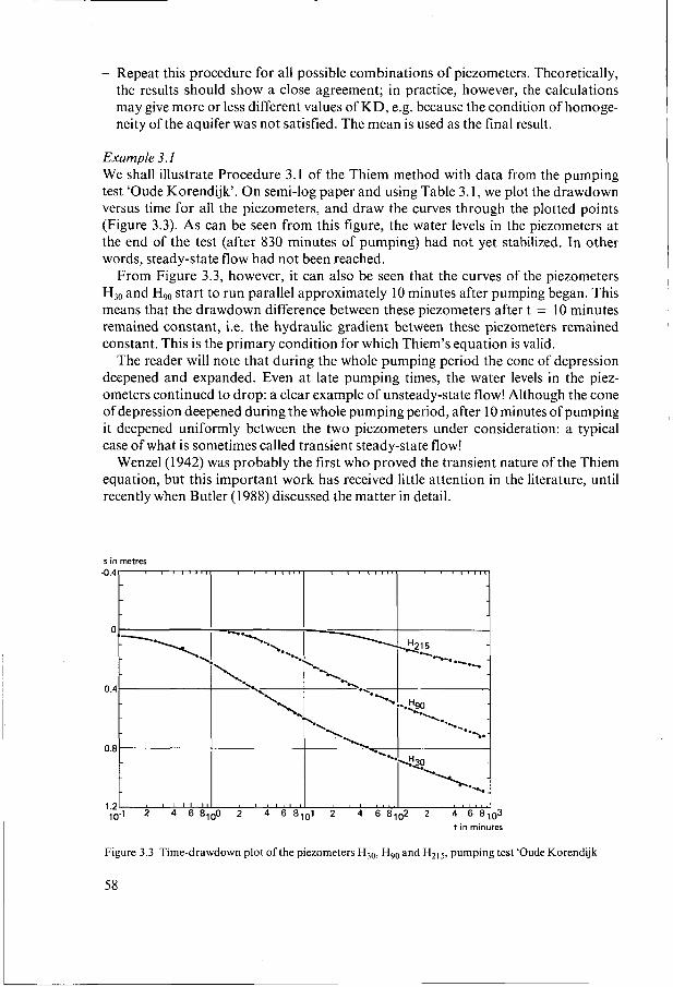
- Repeat this procedure for all possible combinations of piezometers. Theoretically, the results should show a close agreement; in practice, however, the calculations may give more or less different values of KD, e.g. because the condition of homoge- neity of the aquifer was not satisfied. The mean is used as the final result.

Example 3.1 We shall illustrate Procedure 3.1 of the Thiem method with data from the pumping test 'Oude Korendijk'. On semi-log paper and using Table 3. I , we plot the drawdown versus time for all the piezometers, and draw the curves through the plotted points (Figure 3.3). As can be seen from this figure, the water levels in the piezometers at the end of the test (after 830 minutes of pumping) had not yet stabilized. In other words, steady-state flow had not been reached.

From Figure 3.3, however, it can also be seen that the curves of the piezometers H30 and H,, start to run parallel approximately 10 minutes after pumping began. This means that the drawdown difference between these piezometers after t = I O minutes remained constant, i.e. the hydraulic gradient between these piezometers remained constant. This is the primary condition for which Thiem's equation is valid.

The reader will note that during the whole pumping period the cone of depression deepened and expanded. Even at late pumping times, the water levels in the piez- ometers continued to drop: a clear example of unsteady-state flow! Although the cone of depression deepened during the whole pumping period, after 1 O minutes of pumping it deepened uniformly between the two piezometers under consideration: a typical case of what is sometimes called transient steady-state flow!

Wenzel(l942) was probably the first who proved the transient nature of the Thiem equation, but this important work has received little attention in the literature, until recently when Butler (1988) discussed the matter in detail.

s in metres

1.2L ' ' ' ' ' " 1 1 I I J 10.1 2 4 6 8100 2 4 6 8101 2 4 6 8102 2 4 6 8103

t i n minutes

Figure 3.3 Time-drawdown plot of the piezometers H30, H,, and H,,,, pumping test 'Oude Korendijk

58

Table 3.1 Data pumping test ‘Oude Korendijk’ (after Wit 1963)

Piezometer H,, Screen depth 20 m

t(min) s(m) t/r2(min/m2) t (min) s (m) t/r2(min/m2)

O O o. I 0.04 0.25 0.08 0.50 0.13 0.70 0.18 I .o 0.23 I .40 0.28 I .90 0.33 2.33 0.36 2.80 0.39 3.36 0.42 4.00 0.45 5.35 0.50 6.80 0.54 8.3 0.57 8.7 0.58

10.0 0.60 13.1 0.64

O 18 1.11 x 10-4 27 2.78 33 5.56 41 7.78 x IO4 48

1.56 80 2.1 I 95 2.59 139 3.12 181 3.73 245 4.44 300 5.94 360 7.56 480 9.22 600 9.67 x 728 1.11 x 830 1.46 x

1 . 1 1 IO-^ 59

0.680 0.742 0.753 0.779 0.793 0.8 19 0.855 0.873 0.9 I5 0.935 0.966 0.990 I .O07 I .O50 1 .O53 I .O72 I .O88

2.00 x 10-2 3.00 3.67 4.56 5.33 6.56 8.89 x 1.06 x IO-‘ I .54 2.01 2.72 3.33 4.00 5.33 6.67 8.09 9.22 x IO-’

Piezometer H,,

t(min) s(m) t/r2(min/m2) t (min) s (m) t/r2(min/m2)

Screen depth 24 m

2.0 2.16 2.66 3 3.5 4 4.33 5.5 6 7.5 9

13 15 18 25 30

I

O 0.015 0.02 I 0.023 0.044 0.054 0.075 0.090 0.104 0.133 O. 153 O. I78 0.206 0.250 0.275 0.305 0.348 0.364

O 40

2.47 60 2.67 75 3.28 90 3.70 I05 4.32 120 4.94 I50 5.35 I80 6.79 248 7.4 I 30 I 9.26 x IO4 363

I .60 542 I .85 602 2.22 680 3.08 785 3.70 x 845

1.85 x 10-4 53

1 . 1 1 10” 422

0.404 0.429 0.444 0.467 0.494 0.507 0.528 0.550 0.569 0.593 0.614 0.636 0.657 0.679 0.688 0.701 0.718 0.716

4.94 IO-^

9.26 IO-^ 1 . 1 1 x 10-2

6.54 7.41

1.30 1.48 1.85 2.22 3.06 3.72 4.48 5.21 6.69 7.43 8.40 9.69 x 1.04 x IO-’

Piezometer H,,, Screen depth 20 m

t(min) s (m) t/r2(min/m2) t (min) s (m) t/r2(min/m2)

O O O 305 0.196 6.60 w3 66 0.089 1.43 x 366 0.207 7.92 10-3

127 0.138 2.75 x 430 0.214 9.30 x IO-^ I85 0.165 4.00 x IO” 606 0.227 1.31 x IO-2 25 I O. 186 5.43 IO-^ 780 0.250 1.68 x

59

From Figure 3.3, the reader will also note that the time-drawdown curve of piez- ometer H215 does not run parallel to that of the other piezometers, not even at very late pumping times. In applying Procedure 3.1 of the Thiem method, therefore, we shall disregard the data of this piezometer and shall use only the data from the piez- ometers H,, and H,, for t > 10 minutes. In doing so, and using Equation 3.2 after rearranging, we find

90 log - = 370 m2/d 788 x 2.30 2 x 3.14 (1.088 - 0.716) 30 KD =

Similar calculations were made for combinations of these piezometers with the piez- ometer The results are given in Table 3.2. The table shows only minor differences in the results. Our conclusion is that the transmissivity of the tested aquifer is approxi- mately 385 m2/d.

Table 3.2 Results of the application of Thiem’s method, Procedure 3.1, to data from the pumping test ‘Oude Korendijk‘

30 90 1 .O88 0.716 370 0.8 30 2.236 1 .O88 396 0.8 90 2.236 0.716 389

Mean 385

Procedure 3.2 - Plot on semi-log paper the observed transient steady-state drawdown s, of each

piezometer against the distance r between the well and the piezometer (Figure 3.4); - Draw the best-fitting straight line through the plotted points; this is the distance-

drawdown graph; - Determine the slope of this line As,, i.e. the difference of drawdown per log cycle

of r, giving r2/r, = 10 or log r2/rl = 1. In doing so Equation 3.2 reduces to

(3.4) 27tKD 2.30

Q=-

- Substitute the numerical values of Q and Asm into Equation 3.4 and solve for KD.

Example 3.2 Using Procedure 3.2 of the Thiem method, we plot the values of s, and r on semi-log paper (Figure 3.4). We then draw a straight line through the plotted points. Note that the plot of piezometer H215 falls below the straight line and is therefore discarded. The slope of the straight line is equal to a drawdown difference of 0.74 m per log cycle of r. Introducing this value and the value of Q into Equation 3.4 yields

60

sm in metres

2.5

2.0

1.5

1 .o

0.5

O 10 ’ 2 4 6 810’ 2 4 6

I . \

+4 . O

10’ 2 4 6 810’ 2 4 r in metres

Figure 3.4 Analysis of data from pumping test ‘Oude Korendijk’ with the Thiem method, Procedure 3.2

This result agrees very well with the average value obtained with the Thiem method, Procedure 3. I .

Remarks - Steady-state has been defined here as the situation where variations of the drawdown

with time are negligible, or where the hydraulic gradient has become constant. The reader will know, however, that true steady state, i.e. drawdown variations are zero, is impossible in a confined aquifer;

- Field conditions may be such that considerable time is required to reach steady-state flow. Such long pumping times are not always required, however, because transient steady-state flow, i.e. flow under a constant hydraulic gradient, may be reached much earlier as we have shown in Example 3.1.

3.2 Unsteady-state flow

3.2.1 Theis’s method

Theis (1935) was the first to develop a formula for unsteady-state flow that introduces the time factor and the storativity. He noted that when a well penetrating an extensive confined aquifer is pumped at a constant rate, the influence of the discharge extends outward with time. The rate of decline of head, multiplied by the storativity and summed over the area of influence, equals the discharge.

The unsteady-state (or Theis) equation, which was derived from the analogy be- tween the flow of groundwater and the conduction of heat, is written as

61

(3.5)

where S

Q K D

= the drawdown in m measured in a piezometer at a distance r in m

= the constant well discharge in m3/d = the transmissivity of the aquifer in m2/d

from the well

4KDtu and consequently S = ~ r2 r2S u --

- 4KDt S t

= the dimensionless storativity of the aquifer = the time in days since pumping started

W(U) = -0.5772- l n u + u - u2 u3 u4 -+---+... 2.2! 3.3! 4.4!

The exponential integral is written symbolically as W(u), which in this usage is general- ly read ‘well function of u’ or ‘Theis well function’. I t is sometimes found under the symbol -Ei(-u) (Jahnke and Embde 1945). A well function like W(u) and its argument u are also indicated as ‘dimensionless drawdown’ and ‘dimensionless time’, respective- ly. The values for W(u) as u varies are given in Annex 3.1. From Equation 3.5, it will be seen that, if s can be measured for one or more values of r and for several values o f t , and if the well discharge Q is known, S and KD can be determined. The presence of the two unknowns and the nature of the exponential integral make it impossible to effect an explicit solution.

Using Equations 3.5 and 3.6, Theis devised the ‘curve-fitting method’ (Jacob 1940) to determine S and KD. Equation 3.5 can also be written as

logs = log(Q/47~KD) + lOg(W(u))

and Equation 3.6 as

log (r2/t) = log (4KD/S) + log (u)

Since Q/4xKD and 4KD/S are constant, the relation between log s and log (r2/t) must be similar to the relation between log W(u) and log (u). Theis’s curve-fitting method is based on the fact that if s is plotted against r2/t and W(u) against u on the same log-log paper, the resulting curves (the data curve and the type curve, respectively) will be of the same shape, but will be horizontally and vertically offset by the constants Q/4nKD and 4KD/S. The two curves can be made to match. The coordinates of an arbitrary matching point are the related values of s, r2/t, u, and W(u), which can be used to calculate K D and S with Equations 3.5 and 3.6.

Instead of using a plot of W(u) versus (u) (normal type curve) in combination with a data plot of s versus r2/t, it is frequently more convenient to use a plot of W(u) versus l /u (reversed type curve) and a plot of s versus t/r2 (Figure 3.5).

Theis’s curve-fitting method is based on the assumptions listed at the beginning of this chapter and on the following limiting condition: - The flow to the well is in unsteady state, i.e. the drawdown differences with time

are not negligible, nor is the hydraulic gradient constant with time.

62

Procedure 3.3 - Prepare a type curve of the Theis well function on log-log paper by plotting values of W(u) against the arguments ]/u, using Annex 3.1 (Figure 3.5); - Plot the observed data curve s versus t/r2 on another sheet of log-log paper of the same scale; - Superimpose the data curve on the type curve and, keeping the coordinate axes parallel, adjust until a position is found where most of the plotted points of the data curve fall on the type curve (Figure 3.6); - Select an arbitrary match point A on the overlapping portion of the two sheets and read its coordinates W(u), I/u, s, and t/r2. Note that it is not necessary for the match point to be located along the type curve. In fact, calculations are greatly simpli- fied if the point is selected where the coordinates of the type curve are W(u) = 1 and I/u = IO; - Substitute the values of W(u), s, and Q into Equation 3.5 and solve for KD; - Calculate S by substituting the values of KD, t/r2, and u into Equation 3.6.

W ( U )

10 2

6 4

2

101

6 4

2

100

6 4

2

10-1

6 4

2

10-2

6 4

2

6 4

2

6 4

2

lo-' 2 4 6 lob 2 4 6 2 4 6 2 4 6 loe3 2 4 6 lo-' 2 4 6 l o 1 2 4 6 10' 2 4 6 10'u

10-l loo lo1 lo2 lo3 10" 1 o5 1 06 1071,u

Figure 3.5 Theis type curve for W(u) versus u and W(u) versus l/u

63

Figure 3.6 Analysis of data from pumping test ‘Oude Korendijk’ with the Theis method, Procedure 3.3

Remarks - When the hydraulic characteristics have to be calculated separately for each pie-

zometer, a plot of s versus t or s versus I/t for each piezometer is used with a type curve W(u) versus 1 /u or W(u) versus u, respectively;

- In applying the Theis curve-fitting method, and consequently all curve-fitting meth- ods, one should, in general, give less weight to the early data because they may not closely represent the theoretical drawdown equation on which the type curve is based. Among other things, the theoretical equations are based on the assump- tions that the well discharge remains constant and that the release of the water stored in the aquifer is immediate and directly proportional to the rate of decline of the pressure head. In fact, there may be a time lag between the pressure decline and the release of stored water, and initially also the well discharge may vary as the pump is adjusting itself to the changing head. This probably causes initial dis- agreement between theory and actual flow. As the time of pumping extends, these effects are minimized and closer agreement may be attained;

- If the observed data on the logarithmic plot exhibit a flat curvature, several appar- ently good matching positions, depending on personal judgement, may be obtained. In such cases, the graphical solution becomes practically indeterminate and one must resort to other methods.

Example 3.3 The Theis method will be applied to the unsteady-state data from the pumping test

64

‘Oude Korendijk’ listed in Table 3. I . Figure 3.6 shows a plot of the values of s versus t/r2 for the piezometers H3,,, H,, and H,,, matched with the Theis type-curve, W(u) versus l/u. The reader will note that for late pumping times the points do not fall exactly on the type curve. This may be due to leakage effects because the aquifer was not perfectly confined. Note the anomalous drawdown behaviour of piezometer H,,, already noticed in Example 3.2. In the matching procedure, we have discarded the data of this piezometer. The match point A has been so chosen that the value of W(u) = 1 and the value of l/u = 10. On the sheet with the observed data, the match point Ahasthecoordinatess, = 0.16mand(t/r2), = 1.5 x 10-3min/m2 = 1.5 x 10-’/1440 d/m2. Introducing these values and the value of Q = 788 m3/d into Equations 3.5 and 3.6 yields

788 x 1 = 392m2/d 4 x 3.14 x 0.16

and

3.2.2 Jacob’s method

The Jacob method (Cooper and Jacob 1946) is based on the Theis formula, Equation 3.5

From u = r2S/4KDt, it will be seen that u decreases as the time of pumping t increases and the distance from the well r decreases. Accordingly, for drawdown observations made in the near vicinity of the well after a sufficiently long pumping time, the terms beyond In u in the series become so small that they can be neglected. So for small values of u (u < 0.01), the drawdown can be approximated by

r2S (-0.5772-In-) 4KDt s = -

4nKD

with an error less than 1% 2% 5% 10% for u smaller than 0.03 0.05 O. 1 0.15

After being rewritten and changed into decimal logarithms, this equation reduces to

2.304 2.25KDt 4xKDlog r2S

s = - (3.7)

Because Q, KD, and S are constant, if we use drawdown observations at a short dis- tance r from the well, a plot of drawdown s versus the logarithm o f t forms a straight line (Figure 3.7). If this line is extended until it intercepts the time-axis where s = O, the interception point has the coordinates s = O and t = h. Substituting these values into Equation 3.7 gives

65

2.304 2.25KDto 47cKDlog r2S

o = -

= I 2.25KDto rZS and because - 2'30Q # O, it follows that 47cKD

or

2.25KDto r2 S =

The' slope of the straight line (Figure 3.7), i.e. the drawdown difference As per log cycle of time log t/to = I , is equal to 2.30Q/4xKD. Hence

2.30Q 47cAs K D = - (3.9)

Similarly, it can be shown that, for a fixed time t, a plot of s versus r on semi-log paper forms a straight line and the following equations can be derived

2.25KDt S = r;

and

(3.10)

2.30Q 27cAs K D = - (3.1 I )

If all the drawdown data of all piezometers are used, the values of s versus t/r2 can be plotted on semi-log paper. Subsequently, a straight line can be drawn through the

s in metres 1 .O(

o. 5(

O : r - 'i.. =0.375 m

i 10-1 2 4 6 8 IO" 2 4 6 8 10' 2 4 6 810' 2

t in min

Figure 3.7 Analysis of data from pumping test 'Oude Korendijk' (r = 30 m) with the Jacob method, Proce- dure 3.4

66

plotted points. Continuing with the same line of reasoning as above, we derive the following formulas

S = 2.25KD(t/r2), (3.12)

and

2.304 4nAs K D = - (3.13)

Jacob’s straight-line method can be applied in each of the three situations outlined above. (See Procedure 3.4 for r = constant, Procedure 3.5 fort = constant, and Proce- dure 3.6 when values of t/r2 are used in the data plot.) The following assumptions and conditions should be satisfied: - The assumptions listed at the beginning of this chapter; - The flow to the well is in unsteady state; - The values of u are small (u < O.Ol), i.e. r is small and t is sufficiently large.

The condition that u be small in confined aquifers is usually satisfied at moderate distances from the well within an hour or less. The condition u < 0.01 is rather rigid. For a five or even ten times higher value (u < 0.05 and u < O. lo), the error introduced in the result is less than 2 and 5%, respectively. Further, a visual inspection of the graph in the range u < 0.01 and u < 0.1 shows that it is difficult, if not impossible, to indicate precisely where the field data start to deviate from the straight-line relation- ship. For all practical purposes, therefore, we suggest using u < 0.1 as a condition for Jacob’s method.

The reader will note that the use of Equation 3.7 for the determination of the differ- ence in drawdown s, - s2 between two piezometers at distances r, and rz from the well leads to an expression that is identical to the Thiem formula (Equation 3.2).

Procedure 3.4 (for r is constant) - For one of the piezometers, plot the values of s versus the corresponding time t

on semi-log paper (t on logarithmic scale), and draw a straight line through the plotted points (Figure 3.7);

- Extend the straight line until it intercepts the time axis where s = O, and read the value of to;

- Determine the slope of the straight line, i.e. the drawdown difference As per log cycle of time;

- Substitute the values of Q and As into Equation 3.9 and solve for KD. With the known values of KD and to, calculate S from Equation 3.8.

Remarks - Procedure 3.4 should be repeated for other piezometers at moderate distances from

the well. There should be a close agreement between the calculated KD values, as well as between those of S;

- When the values of K D and S are determined, they are introduced into the equation u = r2S/4KDt to check whether u < 0.1, which is a practical condition for the applicability of the Jacob method.

67

Example 3.4 For this example, we use the drawdown data of the piezometer H,, in ‘Oude Korendijk’ (Table 3.1). We plot these data against the corresponding time data on semi-log paper (Figure 3.7), and fit a straight line through the plotted points. The slope of this straight line is measured on the vertical axis As = 0.375 m per log cycle of time. The intercept of the fitted straight line with the absciss (zero-drawdown axis) is to = 0.25 min = 0.25/1440 d. The.discharge rate Q = 788 m3/d. Substitution of these values into Equa- tion 3.9 yields

- - 385m2/d KD=-- 2‘30 788 2 304 47cAs 4 x 3.14 x 0.375 -

and into Equation 3.8

2.25KDto - 2.25 x 385 0.25 x - - 1440 - 302 -

r2 S =

Substitution of the values of KD, S, and r into u = r2S/4KDt shows that, for t > 0.001 d or t > 1.4 min, u < 0.1, as is required. The departure of the time-drawdown curve from the theoretical straight line is probably due to leakage through one of the assumed ‘impermeable’ layers.

The same method applied to the data collected in the piezometer at 90 m gives: KD = 450 m2/d and S = 1.7 x IO4 with u < 0.1 for t > I 1 min. This result is less reliable because few points are available between t = 1 1 min. and the time that leakage probably starts to influence the drawdown data.

Procedure 3.5 ( t is constant) - Plot for a particular time t the values of s versus r on semi-log paper (r on logarithmic

- Extend the straight line until it intercepts the r axis where s = O , and read the value

- Determine the slope of the straight line, i.e. the drawdown difference As per log

- Substitute the values of Q and As into Equation 3.11 and solve for KD. With the

scale), and draw a straight line through the plotted points (Figure 3.8);

of r,;

cycle of r;

known values of KD and r,,, calculate S from Equation 3.10.

Remarks - Note the difference in the denominator of Equations 3.9 and 3.1 1; - The data of at least three piezometers are needed for reliable results; - If the drawdown in the different piezometers is not measured at the same time,

the drawdown at the chosen moment t has to be interpolated from the time-draw- down curve of each piezometer used in Procedure 3.4;

- Procedure 3.5 should be repeated for several values of t. The values of KD thus obtained should agree closely, and the same holds true for values of S.

Example 3.5 Here, we plot the (interpolated) drawdown data from the piezometers of ‘Oude Koren- dijk’ for t = 140 min = O . 1 d against the distances between the piezometers and the well (Figure 3.8). In the previous examples, we explained why we discarded the point

68

s jn metres

m

Figure 3.8 Analysis of data from pumping test ‘Oude Korendijk’ (t = 140 min) with the Jacob method, Procedure 3.5

of piezometer H,,,. The slope of the straight line As = 0.78 m and the intercept with the absciss ra = 450 m..The discharge rate Q = 788 m3/d. Substitution of these values into Equation 3.11 yields

and into Equation 3.10 .. .. i

2.25KDt - 2.25 x 370 x 0.1 = 4.1 - 450, S =

r;;

Procedure 3.6 (based on s versus t/r2 data plot) - Plot the values of s versus t/r2 on semi-log paper (t/r2 on the logarithmic axis), and

- Extend the straight line until it intercepts the t/r2 axis where s = O , and read the

- Determine the slope of the straight line, i.e. the drawdown difference As per log

- Substitute the values of Q and As into Equation 3.13 and solve for KD. Knowing

draw a straight line through the plotted points (Figure 3.9);

value of (t/r2)o;

cycle of t/r2;

the values of KD and ( t / r2k calculate S from Equation 3.12.

Example 3.6 As an example of the Jacob method, Procedure 3.6, we use the values of t/r2 for all the piezometers of ‘Oude Korendijk’ (Table 3.1). In Figure 3.9, the values of s are plotted on semi-log paper against the corresponding values of t/r2. Through those points, and neglecting the points for H,,,, we draw a straight line, which intercepts

69

s in metres

t1r2 in minlm2

Figure 3.9 Analysis of data from pumping test ‘Oude Korendijk’ with the Jacob method, Procedure 3.6

the s = O axis (absciss) in (t/r2),, = 2.45 x IO4 min/m2 or (2.45/1440) x IO4 d/m2. On the vertical axis, we measure the drawdown difference per log cycle of t/r2 as As = 0.33 m. The discharge rate Q = 788 m3/d. Introducing these values into Equation 3.13 gives

K D = - - - = 437m2,d 2.304 2.30 x 788 47cAs 4 x 3.14 x 0.33

and into Equation 3.12

S = 2.25KD(t/r2),, = 2.25 x 437 x - ;zo x IO4 = 1.7 x IO4

3.3 Summary

Using data from the pumping test ‘Oude Korendijk’ (Figure 3.2 and Table 3. I), we have illustrated the methods of analyzing (transient) steady and unsteady flow to a well in a confined aquifer. Table 3.3 summarizes the values we obtained for the aquifer’s hydraulic characteristics. When we compare the results of Table 3.3, we can conclude that the values of KD and S agree very well, except for those of the last two methods. The differences in the results are due to the fact that the late-time data have probably been influenced by leakage and that graphical methods of analysis are never accurate. Minor shifts of the data plot are often possible, giving an equally good match with a type curve, but yielding different values for the aquifer characteristics. The same is true for a semi-log plot whose points do not always fit on a straight line because of measuring

70

errors or otherwise. The analysis of the Jacob 2 method, for example, is weak, because the straight line has been fitted through only two points, the third point, that of the piezometer H,,,, being unreliable. The anomalous behaviour of this far-field piez- ometer may be due to leakage effects, heterogeneity of the aquifer (the transmissivity at H,,, being slightly higher than closer to the well), or faulty construction (partly clogged).

We could thus conclude that the aquifer at ‘Oude Korendijk’ has the following parameters: KD = 390 m2/d and S = 1.7 x lo4.

Table 3.3 Hydraulic characteristics of the confined aquifer at ‘Oude Korendijk’, obtained by the different methods

Method KD S (-1

- Thiem 1 385 Thiem 2 390 Theis 392 1.6 x IO4 Jacob 1 385 1.7 x IO4 Jacob 2 370 4.1 x IO4 Jacob 3 431 1.7 x IO4

-

71