CHUTER 1

Confined Aquatic Disposal Cells

MONITORING BOSTON HARBOR CAD CELLS 3

Monitoring Results from the Boston Harbor Navigation Improvement Project

Confined Aquatic Disposal Cells

T. J. RKDETIE'

P. E. JACKSON

C. J. Roams

U.S. Anny Corps of Engineers, ¹w England District696 Virginia Road, Conc' MA 01742 USA

D. A. HADDEN

Massachusetts Port Authority1 Harborside Drive, Suite 200 South

East Boston, MA 02128 USA

S. H. WOLF

ENSR International

2 Technology Park, Westford, MA 01886 USA

T. A. NOWAK JR.

Ocean Surveys, Inc.91 She/geld St., Old Saybrook, CT 06475 USA

E. DEANt-ELO

Gahagan sfr Bryant, Inc.9008-0 Yellow Brick Road, Baltimore, MD 21237 USA

ABSTRACT: The dredging, filling, and capping of nine Confined Aquatic Disposal CAD! cells for the Boston Harbor Navigation Improvement Project provided an idealopportunity to improve construction methods and monitoring approaches for in-channeldisposal. %'orking with the project Technical Advisory Committee and theMamtchusetts regulatory agencies, it was possible to modify design requirements basedon experiences gained in each successive phase of the project. In 1997, the use andmonitoring of a single CAD cell lead to construction changes in cap placement for thePhase H in-channel disposal cells. Additional experience with the first three, largerPhase H ceHs in 1998 resulted in adoption of recommendations to increase consolidationtime and mhmnixe the use of the props on the hopper dredge during capping. Theseapproaches were applied to the last five cells created by the project in 1999/2000resulting in even higher levels of success than in the earlier cells. CAD cells can providea practicable alternative for contaminated sediment management. The success andexperience gained from projects such as the Boston Harbor Navigation ImprovementProject will certainly increase the enviromnental acceptability of CAD cems as amanagement alternative.

Key words: CAD, capping, monitoring, Boston Harbor, MA

'Corresponding author, telephone: 978-318-8291;fax: 978-318-8303; email: thomas.j.fredettetttusaee.army.mil

4 FREDETTE ET AL.

Note: The findings in this paper were originally pre-sented at the Western Dredging Association, TwentiethDredging Seminar, June 25-28, 2000; Warwick, RhodeIsland, Since the presentation at the December 2000Technical Conference and Twenty-Second Texas ARMConference on Dredged Material Management, a finalsununary report has been prepared US Army Corps ofEngineers, 2002!.

INTRODUCTION

Management of silty, fine grained sediments,determined unsuitable for ocean placement,dredged from the Boston Harbor NavigationImprovement Project BHNIP! have been placedinto a series of confined aquatic disposal CAD!cells dredged below the Federal navigation chan-nels of the inner harbor. Following placement ofthese silty maintenance sechments, sand dredgedfrom the Cape Cod Canal was used to create capsover the cells Figure 1!. Sediments from the cellconstruction and channel deepening were placed atthe offshore Massachusetts Bay Dredged Sediinentsite. This unique, large-scale project has providedan excellent opportunity to improve our under-standing and application of this managementapproach. The latest capping and monitoring, con-ducted at two cells in November and December

1999, have continued to support the conclusion thatconsolidation time is critical to cap success.

Application of the CAD management approachfor the Boston Harbor project has been an evolu-tionary and iterative process that has been coordi-nated with an interagency Technical Advisory

s

>~X/

Figure i. Location of Boston Harbor Navigation ImprovementProject and Cape Cod CanaL

Committee TAC!, Project progress, monitoringresults, and changes in the rnanageinent approacheshave been continually coordinated with the TAC,consisting of local environmental interest groups,academic representatives, federal and state agen-cies. Involvement of these groups throughout theprocess enabled practical project modifications tobe impleinented, as needed, with each new roundof cell capping and monitoring.

The creation of CAD cells for the projectbegan in 1997 when two berths at Conley Terminalwere clainshell dredged and the maintenance sedi-ments were placed using a bottom opening bargeinto a small �00 x 500 ft! and relatively shallow average of -57,5 ft MLLW! ceH Figure 2, cellIC2!. Average fill elevation was -48.5 ft MLLW,resulting in about nine feet of maintenance sedi-ments in the cell. Sand capping began nine daysafter placement of the maintenance sethents andcontinued for 12 days. Results from this first cell referred to as the Phase I cell! demonstrated thatcapping was feasible, though some changes tooperations were recommended. This included arecommendation to not use spudded barges forplacement of cap material, because of the observeduneven distribution of sand over the maintenance

sediments Murray et al. 1999, Murray 1998!. Itwas initiaHy predicted that the sand released fromthe barge would flow downstream with currentswithin the cell. Instead, the sand cap material felldirectly beneath the opening of the barge. It wasalso recommended that a longer consolidation timebe aHowed for the sediment placed in the CAD toreduce the amount of mixing between cap andmaintenance sediments.

The next three cells to be dredged, filled, andcapped M4, M5, and M12! were substantiallydeeper average depths of � 85, � 80, and � 110 ftMLLW! than the Phase I cell Fredette et al, 1999! Figure 2!. These cells were filled with 21, 31, and34 feet of silt, respectively. Consolidation timebetween the last load of maintenance sediment and

the first cap placement ranged from 30 to 52 daysfor these Phase II ceHs, Sand cap was sprinkledusing a partially opened hopper dredge whichmaneuvered over the ceHs. Mixing of sand with thesilt and the presence of silt layers from 1-4 feetthick on top of sand layers over portions of thecells led to the recommendation that even greaterconsolidation time be allowed NB: consolidation

644 M4 6I l4

6 4 6 6II m 6. I 6 . ~ I H «6

6I .6 466

6464 44II6 4464 III 644 III4 46I444I44l

Figure 2. Boston Harbor Navigation Improvement Project, Mysticand Inner Confluence Disposal Cells.

Figure 3. TIme history in days of disposal, open circle!, consolidation,and capping, closed circle!, for Mystic River Cells.

Figure 4. Supercell slump sample average height and spread.

MONITORING BOSTON HARBOR CAD CELLS 5

time was initially determined by the Water QualityCertification goal of minimizing the potentialshort-term environmental exposure, rather thanmaximizing time for capping considerations!.Additional changes in cap placement discussedbelow! were also made to help maximize condi-tions for success.

Since the capping of M4, M5, and M12, fiveother cells have been under active use. Four of

these, Supercell, M2, M8 and M19, are in theMystic River and one, C12 not shown!, is in theChelsea River, This paper discusses the resultsfrom the cells capped late in 1999, M2 and theSupercell. Of the remaining cells, M8 and M12were capped in the fall of 2000 and monitoringresults are currently being reviewed. As cell C12was only partially filled, it will remain uncappedand available for future projects.

FILLING AND CAPPING OF CELL M12AND SUPERCELL

Cells M2 and the Supercell so called, becauseof its size! had very different time histories thanthe prior three cells M4, M5, and M12 Figure 3!.These two cells had considerably greater consoli-dation times approximately 5 months! and alsohad inore prolonged placement of the silty mainte-nance sediments. Silt placement into M4, MS, andM12 took place in less than 45 days time, whereasthe filling of the SuperceU and M2 stretched over 6and 8 months, respectively, Average cell depths forM2 and the Superceii were similar to the earlierPhase II cells, but the Supercell was considerablylarger in footprint Figure 2!.

As part of assessing the readiness of the cellsfor capping, a simple slump test was used to exam-ine changes in silt consolidation. This was done bytaking three sediment grab samples periodicallyfrom each cell, placing the grab on a sheet of ply-wood pre-marked with concentric circles, and esti-mating the spread and height that the sedimentmaintained. Both qualitatively and quantitativelythese samples provided some evidence of increasedconsolidation through time. The height that thematerial maintained showed a fairly clear trend,whereas the spread was more equivocal Figure 4!,

Capping of M2 and the Supercell used the hop-per dredge, Sugar Island Great Lakes Dredge and

6 FREDETTE ET AL

MOMTORING METHODS

r*

rS,.;

.922

CAtt catt Fil! Depthsss':c 5

nuns; o.Ael

Jl' I MSl~

Dock Company!, that was opened just enough toslowly release the sand. However, for these twocells the dredge was maneuvered using a tug ratherthan utilizing the dredge's own engines as wasdone for the previous three cells. 1'his change wasmade as one more means to minimize any potentialfor disturbance of the silt during capping, Sevenhopper loads of sand �7,500 yd3! were placedover M2 and 20 over the Supercell �9,700 yd3!.As for the previous three cells Fredette et al.1999!, dredge position was recorded every ten sec-onds during cap placement of each load and thesedata were used to estimate cap coverage. Dredgeposition was displayed as a line representing thelongitudinal axis of the dredge. This is shown for asingle cap load in Figure 5 and similar data fromall of the cap loads were subsequently combined toestimate cap thickness as construction proceeded.

Disposal Positions t 0 sec interval!

RFs '.: "=.' . FN-.c rstr."': assn n nn, o nsl o.':::ll!

o -Kg

Figure 5. Position of hopper dredge during placement of load ¹4into cell M2 top! and estimated cap thiclcness from the single load bottom!.

Sub-bottom profiling and coring of the cellswas conducted by Ocean Surveys, Inc. within twoweeks of capping using the same equipment andapproaches described earlier Fredette et al. 1999!.Cell M2 was surveyed on two longitudinal tran-sects and four lateral transects Figure 6!.Surveying the larger Supercell involved four longi-tudinal sections and eight cross sections. Six andfifteen vibracores, respectively, were taken at inter-secting points of the sub-bottom survey lanes toallow better interpretation of these two data types.Previously, it had been recommended that cores berandomly located Fredette et al. 1999!. However,additional discussion of the data from the previouscells led to the conclusion that coordination of

these two data sets would strengthen the overallanalysis.

4

A

s

C'

Figure 6. Sub-bottom survey lanes and core locations for cell M2 top! and the Supercell bottom!.

RESULTS

Sn+c lc a

c.S tea

trace,Isn-s

I

IcI M~

c.c

ceca

DrscUSStoN

acc .'

Sub-bottom profiles of cells M2 and theSupercell showed a strong reflective layer at thesurface of the cell indicative of a sand cap Figure7!. Below the sand cap was the relatively feature-less silty sediments, The sand caps showed consid-erable medium and large scale topographic varia-tion and occasional internal layering, somethingnot seen in the first three cells, because of theamount of silt mixed with the sand cap, TheSupercell was also characterized by the presence ofmultiple diapiric structures, which appear asupward arching features in the cap Figure 8!.These diapiric structures, which are similar tothose observed in geologic records, possibly werecaused by movement of water or silt, These struc-tures were almost non-existent in cell M2.

The cores provided direct physical evidence ofthe presence of the sand cap at the surface of the

~ c ~g

Figure 7. Sub-bottom profile line x of cell M2 showing cap andlocation of two cores.

lPc cI I

Ecru ' KSI-uc

Figure S. Sub-bottom profile along line 3 of the Supercell showingcore locations and numerous silt diapirs.

MONITORING BOSTON HARBOR CAD CELLS 7

cells Figure 9!. Most cores from the two cellsshowed sand from 1-4 feet thick at the sediment-

water interface � of 6 in cell M2 and 12 of 15 in

the Supercell!. A few of the cores showed no sandat the surface e.g., SS1-2, SS1-14, M2-4! and sev-eral had multiple bands of sand separated by layersof finer silty sediments e.g., SS1-2, SS1-11, M2-5!,

Figure 9. Core descriptions from cell M2. Sand is shown as stippled,silt as black and Boston blue clay BBC! as gray. Units are in feet.

Both the Supercell and cell M2 appeared tohave continuous sand caps ranging from one tofour feet thick over the silty maintenance sedi-ments. The M2 cap most closely matches idealexpectations, with little evidence of diapirism andmore consistently thick surface sand layers in thecores. The Supercell had numerous diapiric struc-tures, which appear as upward arching features onthe sub-bottom profiles Figure 8!. Cores thatshowed no sand at the surface almost alwaysappeared to be associated with the presence of oneof these diapirs, For example, core SS1-2 wastaken along the Supercell transect Line 2 where thepresence of a diapir was clearly evident Figure10!. Creation of these diapiric features may becaused by silts trying to move through the cap or

FREDETTE ET AL.

sa:1, 'tssr.' ,Ssl-2

Iarnot > t'<suc�c t 9 l ial-I s

25 meters; 75 tt

Islit

V + diapir

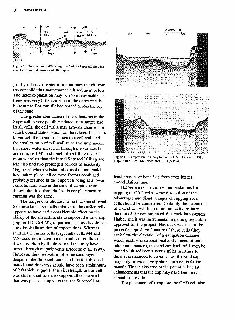
Figure 10. Sub-bottom profile along line 2 of the Supercell showingcore locations and presence of silt diapirs.

just by release of water as it continues to exit fromthe consolidating maintenance silt sediment below.The latter explanation may be more reasonable, asthere was very little evidence in the cores or sub-bottom profiles that silt had spread across the topof the sand.

The greater abundance of these features in theSuperceH is very possibly related to its larger size.In aH cells, the cell walls may provide channels inwhich consolidation water can be released, but in alarger cell the greater distance to a cell wall andthe smaller ratio of cell wall to cell volume means

that more water must exit through the surface. Inaddition, ceH M2 had much of its filling occur 2months earlier than the initial SuperceH filling andM2 also had two prolonged periods of inactivity Figure 3! where substantial consolidation couldhave taken place. AH of these factors combinedprobably resulted in the SuperceH being at a lowerconsolidation state at the time of capping eventhough the time from the last barge placement tocapping was the same.

The longer consolidation time that was allowedfor these latest two cells relative to the earlier cells

appears to have had a considerable effect on theability of the silt sediments to support the sand cap Figure 11!. CeH M2, in particular, provides almosta textbook illustration of expectations, Whereassand in the earlier ceHs especiaHy cells M4 andM5! occurred in continuous bands across the ceHs,it was overlain by fluidized mud that may haveoozed through diapiric vents Fredette et al. 1999!.However, the observation of some sand layersdeeper in the SuperceH cores and the fact that esti-mated sand thickness should have been a minimum

of 2 ft thick, suggests that silt strength in this cellwas stiH not sufficient to support all of the sandthat was placed. It appears that the SuperceH, at

Figure 11. Comparison of survey line 40, cell MS, December 1998 top! to line 3, cell M2, November 1999 below!.

least, may have benefited from even longerconsolidation time.

Before we refine our recommendations for

capping of CAD cells, some discussion of theadvantages and disadvantages of capping suchcells should be considered. Certainly the placementof a sand cap will help to minimize the re-intro-duction of the contaminated silts back into Boston

Harbor and it was instrumental in gaining regulatoryapproval for the project. However, because of theprobable depositional nature of these cells theyare below the elevation of a navigation channelwhich itself was depositional and in need of peri-odic maintenance!, the sand cap itself will soon bebtuied with sediments very similar in nature tothose it is intended to cover, Thus, the sand capmay only provide a very short-term net isolationbenefit. This is also true of the potential habitatenhancements that the cap may have been envi-sioned to provide.

The placement of a cap into the CAD cell also

MONITORING BOSTON HARBOR CAD CELLS 9

has a negative value with respect to cell capacity.Without the cap the cell can accommodate an evengreater volume or the cell capacity used by a capcan simply be left to accumulate future deposition.This behavior as a segment trap could have along-term benefit with respect to decreasing thevolume or frequency of future channel mainte-nance. This would both decrease the regulatorychallenges of future maintenance needs and alsolessen the environinental disturbance that occurs

with dredging.There are also other concerns that factor into

the use of CADs and their capping, including thepotential to create anoxic sinks and the impacts oflarge vessels on erosion of cell contents. Both ofthese have been considered in Boston and relevant

investigations have been conducted. Sampling con-ducted in 1999 did not observe lower dissolved

oxygen in the Boston CAD cells NormandeauAssociates, Inc. 2000!, but this is an issue that mayneed further investigation to reach any long-termdefinitive conclusion. Anoxia development mayalso be a very locale-specific issue for which someverification monitoring may be appropriate.

An investigation was performed in the springof 2000 to provide an initial evaluation of theeG'ect of vessel passage over capped and uncappedcells SAIC, 2000!. Currents and suspended solidswere monitored in the water column over the cells

following passage of a large vessel, The monitor-ing revealed that bottom sediments were temporari-ly resuspended with the passage of the vessel, butthe amount of sediment resuspended was verysmall. It needs to be recognized that the same sedi-ments that are cause for concern in the CAD cell

may be the same segments that were even closerto prop wash disturbance when they were in thechannel in a shallower situation.

RECOMMENDATIONS

Confined Aquatic Disposal CAD! cells offer apractical and effective alternative for the manage-ment of contaminated sediments. However, thereare several questions that need to be consideredbefore their selection for project use. One of themost critical, for design purposes, is the necessityfor a cap. If the benefits of a cap are determined tobe less than the disadvantages, then consideration

of consolidation time and choice of dredgingeqmpment take on less importance. Disadvantagesof a cap include the loss of cell capacity that thecap uses and the cost associated with supplyingcap, while the advantages may include isolationwhere rapid sediment accumulation over the cap isnot anticipated.

If the use of a cap is determined necessary,then using approaches that maximize the strengthof the underlying sediments becomes a large con-sideration. This includes the method used to dredgethe sediments and the length of tiine that consoli-dation will be allowed prior to capping. Also to beconsidered is the choice of cap material and themethod used to place the cap. If erosion of thematerial in the CAD is of concern then a coarse

cap may be required. Sand, because of its greaterdensity, however, may not be the best choice for acap over silty, high water content sediments. Slurryplacement of a fine grained, clean silty sedimentcould eliminate the need to allow consolidation and

also lessen concerns about impacts of dredge selec-tion on sedunent strength. The relative density andstrength thfferences between a maintenance silt anda silty cap would likely result in very little mixingand effective capping. Though, as learned severalyears ago in the New Bedford Harbor pilot project,mixing of such similar materials can occur if thecap is discharged with too much energy directlynear the CAD fill elevation US Army Corps ofEngineers 1990!. Even gradual disposal from abarge of similar high water content silt segmentsmay lessen the need for consolidation.

The Boston Harbor CAD cells represent themost extensive use of this alternative in the United

States and internationally it is probably secondonly to their use in Hong Kong Whiteside et al.1996!. However, the monitoring that has been con-ducted on the Boston cells is likely more extensivethan that conducted elsewhere. With the growingconsideration of the use of CAD cells throughoutthe world we offer the following suggestions:~ Evaluate whether a cap is necessary and

advantageous. Its benefits may be short-term atbest because of rapid new sedimentation.

~ Maximize the strength of the fill sediinents bydredging thein as close to in-situ density aspossible. This may include avoiding the use ofhydraulic dredges or water-tight clamshell

10 EREDETTE ET AL.

buckets which may introduce excess water intothe sedunent.

Bathymetric surveying is of limited use inassessing cap thickness, because of the ongoingelevation changes that occur due to consolida-tion of the sediments.

Coring, combined with sub-bottom profiling,can be an effective means of monitoring capsuccess. Together these methods were verycomplementary, whereas alone they wouldhave been much more difficult to interpret,Placement of core locations at intersectingpoints of the sub-bottom suey lanes provedof much greater use than randomly selectedlocations.

Use of gradual cap placement and a tug tomaneuver the hopper dredge are both potentialmeans tO help tnininiize miXing Of Cap and thecontaminated sediments,

Disposal of the silty material into the CADcells from hopper or split hull barges can beaccomplished successfully with little impact towater quality,Consolidation times of 5-6 months or longermay be needed for cells of similar dimensionsand using similar fill and cap materials as inBoston. However, the length of time to fill thecell should also be considered. If filling occursquickly, longer consolidation tilnes of up to ayear prior to capping may be reasonable.

LIYKRArmz CITED

Fredette, T. J., P. E. Jackson, P. M. Murray, D. A. Hadden, and D. LBeru 1999. Preliminary monitoring msults fi om the phase IlBoston Harbor confined aquatic disposal cells. In Proceedings ofthe Western Dredging Association, Nineteenth TechnicalConference and Twenty ftrst Texas A&M Dredging Seminar, May15-18, 1999, Louisville, KY. pp. 255-275.

Murray, P. M., T, J. Fredette, P. E, Jackson, S. H. Wolf, and J. HRyther, Jr. 1998. Monitoring results from the first Boston HarborNavigation Improvement Project confined aquatic disposal ceII.In Proceedings, 15th World Dredging Congn;ss, WODCONXV,Las Vegas, NV, June 28- July 2, 1998. Vol 1. World Organizationof Dredging Associations WODA!. Ed; R. E, Randall, pp.415-430.

Murray, P. M. 1999. Monitonng Results from the First BostonHarbor Navigation Improvement Project Confined AquaticDisposal Cell. Contribution ¹124, Disposal Area MonitoringSystem DAMOS!. US Army Corps of Engineers, New EngiandDistrict, Concord, MA, 43 pp,

Normandeau Associates, Inc. 2000. Dissolved oxygen near the bot-tom in disposal cells M4, MS and M12 and the adj acent sites inthe Mystic River, Report submitted to the New England District,

US Army Corps of Engineers. Concord, MA.SAIC, 2000. Boston Harbor Water Quality Monitoring � Vessel

Passage over Confined Aquatic Disposal Cells � Monitoring inthe Wake of LIVG Carrier Matthew on March 31, 2000, Reportsubmitted to the New England District, US Army Corps ofEngineers. Concord, MA.

Whiteside, P., K. Ng, and W. Lee. 1996. Management of contaminat-ed mud in Hong Kong, Terra et Aqua 65: 10-17.

US Atmy Corps of Engineers, 2002. Boston Harbor NavigationImprovement Project � Phase 2 Summary Report. ~ by;ENSR Inuunational under contract DACW33-96-D004, May,2002.

US Army Corps of Engineers. 1990. New Bedford Harbor SuperfundPilot Study: Evaluation of Dredging and Dredged MaterialDisposal. US Army Corps of Engineers, New Enghnd Division,Waltham, MA.

PARTICLE CLOUD DYNAMICS

Dyn:mdcs of Particle Clouds Related to Open-Water Sediment Disposal

GORDON J. RVOr~Ht

E, Emc ADAMs'

Department of Civil and Environmental EngineeringMassachusetts Institute of Technology, 48-325Cambridge, MA 02139 USA

ABSTRACT: Open-water disposal and capping are promising solutions for disposal ofthe 14 to 28 mullion cubic meters of contaminated sediment dredged annually in theUnited States. However, such practices raise concerns about the feasibility of accuratelyplacing the material in a targeted area and the loss of material to the environmentduring disposaL

To investigate the question of sediment loss during disposal, laboratory experimentswere conducted in a deep glass-walled tank usmg a quick-opening sediment releasemechanism and a specially<esigned curtain shade serving as a "sedunent "trap". Bothnon-cohesive and cohesive sediments were utiTized under a variety of release conditions varying initial momentum, water content, initial stirring, etc.!. Data co~ of digitalimages of particle douds illuminated by laser-induced fluorescence, and measurementof sediment mass captured on the trap at various stages of cloud descent. The majorcause for particle loss was observed to be failure of material to be incorporated into theplume, rather than any observed "stripping" mechanism.

Current particle cloud models employ thermal theory and an integral approach usingconstant entrainment tX!, drag C<! and added mass k! coefricients. Our aim was toinvestigate how real sediment characteristics particle size, water content and initialmomentum! affect doud behavior and hence ttme variations in C, Cd, and k.

Key words: particle dispersal, open-water disposal, cloud behavior

INTRODUCTION

Corresponding author, telephone: 617-253-6595;fax: 6l7-258-8850; email: eeadann Omit.edu

Open-water disposal, with or without capping,is a promising solution for disposing of the 14-28million m' of contaminated sediment dredgedannually in the United States NRC, 1997!.However, such disposal raises concerns about theability to accurately place sediments either con-taminated dredged material or clean capping mate-rial! in a targeted area, as well as the loss of sedi-ments to the environment during disposal.

Instantaneously released sethrnents formaxisyrnmetric "clouds" resembling self-similarthermals. Current particle cloud models such asSTFATE Johnson and Fong, 1995! date back toKoh and Chang �973!. Most models employ

thermal theory with an integral approach usingconstant entrainment spreading rate! tx!, drag Cd> and added mass k! coefficients. Our aim wasto see how real sediment characteristics particlesize, water content and initial momentum! affectcloud behavior and hence time variations in a, Cdand k, especially in the initial phases of plumedescent of particular relevance to shallow watersites see Figure 1!. We were also concerned withthe process of cloud formation, and with measur-ing how much of the material is initially incorpo-rated into the cloud, as well as how much is lost

during convective descent.

Flow visualization experiments were conductedby releasing 40 g dry wt.! of either non-cohesive

12 RDGGABER 4 ADAMS

Nc = ws r/ B/p!1/2

ANmvsrs

Velocity

Figure i. Phases in the convective descent of an idealized Particlecloud.

glass beads, or cohesive ground silica silt lessthan 36% solids by wt.!. Experiments were con-ducted in an 8-ft-deep glass-walled tank, using aquick-opening sechment release mechanism and awindow-shade type "trap" mechanism Ruggaber,2000!. Observations were recorded using a CCDcamera and framegrabber image system for subse-quent image processing.

Cloud momentum was varied by changing theheight-diameter ratio of the release cylinder, thecylinder's distance above the water surface, and theamount of excess water. Conditions for three

groups of experiments are illustrated in Table 1.Particle sizes were scaled to real-world dimensions

Table 2! through the cloud number N,! defined asthe ratio of the particle settling velocity ws to thecharacteristic cloud velocity,

where B, r and p are cloud buoyancy, radius anddensity Rahimipour and Wilkinson, 1992!.

A simple integral-type model was employed todetermine the ability of this class of model to sim-ulate cloud behavior within the initial acceleration

and deceleration phases. The model solves the

mass, momentum, and buoyancy conservationequations for a cloud of constant shape using eitherconstant or time-varying values for ot, Cd, and k.An "inverse" integral model was also developed inwhich the conservation equations were solved fortwo of the three input parameters e.g., tx and k!based on measured time variation in cloud velocity w! and equivalent radius r!. Based on the inversemodel results, parole cloud experiments weresimulated with an integral model using constantand time-varying tx, Cd, and k.

RESULTS FOR MODEL PETERS

Table 3 summarizes results for cloud growthfor the experiments described in Table 1. Non-cohesive sediments rapidly formed "turbulent ther-mals" with asymptotic deceleration w - t '~;Figure 2! and large initial growth rates �.2 < ctt0,3!. The particles eventuaHy evolved into "circu-lating thermals" with linear growth rate predictedby buoyant vortex ring theory cd � B/K'! where Kis the cloud circulation Ruggaber, 2000!. Thistransition was observed when the cloud radius had

approximately doubled relative to its initial sub-rnerged radius or quadrupled relative to its pre-release radius. This follows boundary layer theoryand corresponds to field water depths of order 100 mIn the "circulating therinal" phase, large particles N ! 10 ! produced laminar-like vortex rings withsignificantly slower spreading �.1 ct 0.2!,while the smaller particles maintained close to theiroriginal a values Figure 3!. Changes in watercontent and initial momentum produced more vari-ation in the spreading of cohesive particles as com-pared with non-cohesive particles.

Inverse integral modeling suggests that C< andk are near zero within the "turbulent thermal"

phase. In the "circulating thermal" phase, the reduc-tion in a caused by the large particles Nc>10 !increased k to a value similar to that of a solid

sphere -0.5!. Integral model results confirm thesuitability of using constant coefficients for model-ing particle clouds with N, < 10+, while forN,0+, time-varying a and k are required toproperly simulate cloud behavior in the "circulatingthermal" regime.

PARTICLE CLOUD DYNAMICS 13

Table l. Conditions for three groups of experiments. Bold entries are varied within each group.

Part. Ia. Part. set. Cyl. dia. Cyl. ht;/dia. mm! veL cm! ratio

cm/s!

Excess Rel. pos.H20 cm'!

Experiment

Group I Experiments

0.264 3.2 3.18

0.264 3.2 3.180.264 32 4.450.264 3.2 4.45

Group II Experiments

0264 3.2 4.45

0.264 32 4,45

0,264 32 4.45

0.264 3.2 4.45

40 AW

40 BW

40 AW

17 AW

Group ID Experiments

0.024 0.047 4.450.024 0.047 4.450.010 0.0091 4.450.010 0.0091 4.45

sko64 mn ssaassa, AwTable 2. Nc scaling of particle cloud grain sizes between 27 cmlaboratory volume and barge volumes of 10, 100, 1000 and 5000 ms.

0

10

6 10 16 20Radltsa tom!

0.010 mm Slit. AW

1.6

101.4

0.6

0 0.2 OA 0.6 0%Log rsna!

Figure 2. Cloud velocity vs. time for Group 11 Experiments, The-0.5 slope matches thermal theory.

0 5 10 16 20Racaua stash .

Figure 3. The entrainment coefEcient s~g rate! for two Gmupm Experiments.

3,18 cm cyl., dry

3.18 cm cyl,, wet4,45 cm cyl., dry4.45 cm cyl�wet

40cm H20, Sus.,AW40cm H20, Sus.,BW40 cm' H20, Sus., AW17 cm' H20, Sus., AW

0.024 mm beads, AW0.024 mm beads, BW0.010 mm beads, AW0.0I0 mm beads, BW

1.1

1.30.40.5

0.8

0.8

0.8

0.5

0.80,80,80.8

0

17017

40404040

AW

AWAWAW

AWBWAWBW

14 RDGGABBR k ADAMS

Table 3. Cloud growth parameters for experiments shown in Table 1. Time t, denotes the onset of turbulence corresponding approximately tofully submerged conditions!; t, and z denote the time and depth associated with the transition to "circulating thermal"; at and tx2 ate spreadingrates before and after this transition, and r, rt and r are equivalent cloud radii before release, at the onset of turbulence and at the transition tocirculation.

a. It's! Qs! z, cm! r Jr, r Jr,Experiment

Group I Experiments

3.18 cm cyl., dry3.18 cm cyl., wet4 45 cm cyl., dry4.45 cm cyl.�wet

0. 14 0.5 1.7G.! 8 0.27 '2.30.16 0.47 1.30.14 0.30 1.3

0,180.170.200.22

39513126

2.0 4,53.3 5.11.9 4,12.3 3.9

Group 11 Experiments

40 cm H2O, Sus,, AW40 cm' H20, Sus., 8 W40 cm' H20, Sus,, AW17 cm' H20, Sus., A W

G.18 0.13 1.0G. I 8 0.40 !.40.16 0.20 1.40.19 0.17 1.1

0.270290.230.3 I

19232822

23 332.0 3.82,4 3.92.7 4.0

Group 111 Experiments

0.23 0.12 020 3.0028 02G OAG 2 70.27 0.2G 0.13 5.20.29 024 027 2.6

2.8 5.42.6 4.56.8 6.84.8 4.8

0.024 mm beads, A W0.024 mm beads, BW0.010 mm beads, A W0.010 mm beads, BW

3&295533

the bottom shortly after it. Material not incorporatedinto the "stem", which may be advected by arnbi-ent currents, was found to be only a small fraction < 1%! of the original mass.

CQNcLUsloNs

Figure 4. Sediment trap locations for determining "stem" massdistribution for 0,010 mm "BW" silt experiment.

LOSS OF FINES

ACKNOWZXaX:MENTS

This study was supported by the MIT Sea GrantCollege Program contract no: NA86RGO074! andthe New England Division of the U.S. Army Corpsof Engineers, through SAIC contnct no: 4400039096!,

Sediment trap experiments indicated that fail-ure of particles and fluid to be initially incorporat-ed into the cloud represents the main mechanismthrough which sediment is lost to the environment.Material not initially incorporated into the cloudformed a narrow "stem" behind the cloud, whichcontained as much as 30% of the original massdepending on the release conditions see Figure 4!.Sediment collected on traps placed at differentdepths relative to the passing cloud showed thatmuch of the "stem" material was either re-entrained into the cloud later in descent or reached

Particle clouds transition from an initial

"turbulent thermal" regime to a "circulating ther-mal" regime when their radius grows by about afactor of four relative to the prerelease radius.Fine particles N < 10+! exhibit constant spreadingthroughout both regimes characterized by �.2 < ct< 0.3!, but significant sensitivity to initial watercontent and momentum. Larger particles exhibit adecrease in spreading from 0.2 < cl < 0,3 to 0.1 <a < 0.2 following the transition, For water depthsgreater than about 100 m, this variation should beincluded in model simulation. Finally, the majorcause for particle loss is failure of material to beincorporated into the plume, rather than anyobserved "stripping" mechanism.

PARTIcLE cLouD DYNAMIcs 15

LrrZRATURK CITKD

Johnson, B.H. and M.T. Fong. 199S. Development and vertfication ofnumerical models for predicting the initial fate of dredged mate-rial disposal in open water, Report 2, Theoretical developmentsand verification results. Technical Report DRP-93-1. FinalReport, U,S, Army Corps of Engineers Watervvays ExperimentStation. Vicksburg, MS.

Koh, R.C.Y. and YC. Chang. 1973. Mathematical model for bargedocean disposal of waste. Environmental Protection TechnologySeries EPA 660/2-73-029. U.S. Army Corps of EngineersWaterways Experiment Station. Vicksburg, MS.

NRC National Research Council!. 1997. Contaminated Sediments inPons and Waterways, Cleanup strategies and Technologies.Committee on Contaminated Marine Sediments. NationalAcademy Press. Washington, DC.

Rahimipour, H. and D. Wilkinson. 1992. Dynamic behavior of parti-cle clouds. In Proc. 11th Australasian Fluid Mechanics Conf.Univ. of Tasmania Hobart, Australia.

Ruggaber, G J. 2000. Dynamics of Panicle Clouds Related to Open-Water Sediment DisposaL Ph.D. Thesis. Dept. of Civil andEnvironmental Engineering, MIT.

16 PEMBRoRE a BAJER

Disposal of Boston Harbor Sediments into in-Harbor CADS:

Minimal Water Quality Effects

ANN PEMl3ROKE'

JAMEs BAlEK

Normandeau Associates, Irtc.

25 Nashua Rd.

Bedford, NH 03110 USA

ABSTRACT: Maintenance and improvement dredging of portions of the federalchannels servicing Boston Harbor MA!, as well as adjacent berth areas occurred fromsummer 1998 until spring 2000. Maintenance material approxiniately 1,000,000 cy! wasfound to be unsuitable for unconfined open water disposal during the environmentalimpact asssmment process. Assessment of disposal alternatives identified areas withinthe footprint of the federal navigation channel upstream of subsurface obstructions vehicular tunnels! as the preferred option for constructing deep cells for containing thedredged silt material. Water quality modeling, using worst~ assumptions, duringthe environmental impact as!essment process indicated that this type of disposal couldbe accomplished with nnimnal water quality impacts. Permit requirements weredeveloped to include a water quality monitoring prograin that tested the variousdisposal scenarios that were anticipated to arise. This paper details the results of themonitoring program.

The monitoring program included tracking of the turbidity plume that was predicted toresult from disposal from each scow. In addition, various sediment sources specificchannels and berths! and disposal locations were targeted for turbidity and waterchemistry monitoring. These scenarios were selected to be representative of the typicalproject conditions as well as the worst-case conditions. In most cases, the disposal plmnewas so negligible that it was difncult to identify. No parameters tested were found toexceed applicable water quality criteria. It is concluded, therefore, that, as predicted,maintenance dredging of portions of Boston Harbor was accomplished with nosubstantial water quality effects.

Key words: CAD, water quality monitoring, turbidity plume, impact assessinent,contaimnated sediments

BACKGROUND

Surficial sediments lrom the channels and

berths proposed for deepening were extensivelytested for chemical and physical properties, biolog-ical effects and water column effects during thedeveloping of the draft EIR/S for the BostonHarbor Navigation Improvement and BerthDredging Project BHNIP!. Results are detailed inthe DEIR/S Massachusetts Port Authority and

Corresponding author; telephone: �03-472-5101!;fax: �03-472-7052!; email; apembroke 4'normandeau.corn

U.S. Army Corps of Engineers 1994!. Coinparisonof chemical and physical results to theMassachusetts Department of EnvironmentalProtection MDEP! standards for assessing dredg-ing material disposal options showed that mostsurface sediments exceeded the allowable limits

for unconfined open water disposal. Furtherbioassay testing indicated that the potential forsublethal effects existed. Thus, it was determinedthat none of the surface sediments could be dis-

posed at the Massachusetts Bay Disposal Site.Excavation of deep cells within the BHNIP

footprint in the federal channels was identified as

WATER Q'VALtTY EFFECTS 17

the most environmentally sound disposal option Massport and USACE 1995!. On the plus side,contaminated sediments would remain near the

source; and, capping would sequester contami-nants. Soine concerns remained, however.

Elutriate results had indicated that some parameterscould be dissolved in the water column during dis-posal Massport and USACE 1994!. As BostonHarbor has been experiencing dramatic improve-ments in water quality as a result of MassachusettsWater Resotuces Authority's MWRA! activities reductions in CSOs, cessation of sewage sludgedisposal!, there was a concern that disposal in-harbor could impair these improvements, eventemporarily.

Water quality effects of disposal in BostonHarbor were evaluated during the EHVS processusing a combination of the STFATE and WQMAPmodels ASA 1995!. Assuming that disposal ofsethments containing the highest concentrations ofcontaminants observed took place in a single loca-tion in the harbor on a daily basis, the model pre-dicted that a steady-state would develop in whichan area of slightly increased suspended segmentsand slightly elevated but below water quality cri-teria! concentrations of parameters such as copper,mercury and PCBs would persist until disposal wascompleted. Plume dimensions would vary accord-ing to the tide, with gradual dispersion down theharbor.

To address the concern that flood tides would

cause waterborne disposed sediments to build up inthe upper inner harbor and to allow the largest vol-ume of water for dilution, MDEP required that thedredger dispose only around high slack tide. Inaddition, they established a water quality monitor-ing plan to assess the areal extent of the influenceof individual and cumulative disposal events.Various situations triggered monitoring, including:early disposal episodes in each tributary Mysticand Chelsea Rivers!, disposal of high volumes ofsediments on a given tide, disposal of the morehighly contaminated berth sediments, and limitedremaining capacity of a cell.

MowrroRtNG CoMpoNENTs

Four types of monitoring were conducted:areal extent of the turbidity plume, water quality atthe edge of the inixing zone, dissolved oxygen in

bottom waters above uncapped cells, and bioaccu-mulation Table 1!. For the turbidity pltune track-ing and turbidity measurements during water quali-ty monitoring, data were collected using a YSI6920 turbidometer interfaced with differential GPS

using HydroPro software that recorded turbidityand position at one-second intervals approximatelyevery 2-5 feet traveled!.

Table l. Monitoring components, as required by the MassachusettsDepartment of Environmental protection Water Quality Certificate.

Water quahty monitoring was initiated bydetermining the location of the densest portion ofthe plume both laterally and vertically along a tran-sect 300 ft downcurrent of the disposal cell. Thiswas accomplished by towing a turbidometer alongthe transect extending 200 ft beyond the sides ofthe cell within three feet of the bottom and in the

middle of the water column. Turbidity, depth, andDGPS coordinates were displayed and recordedcontinuously during these tows. The location ofthe highest turbidity readings was reoccupied andconfirmed by collecting a vertical turbidity profile,Water samples were collected at this site. Duringeach water quality monitoring event, a series offive samples was collected Table 2!. Figure 1shows the layout of the sampling stations for atypical water quality monitoring event. Waterchemistry results were compared to the water qualitycriteria developed by MDEP. Samples collected 0.5and 1.0 hour after disposal were compared to theacute criteria. Samples &om 4-6 hours after disposal

18 PEMBRoKE a BAJEK

WATER QvALrrv

DIssoivED OxvrEN

were compared to the chronic criteria. Dissolvedoxygen immediately above the bottom was collect-ed in order to ascertain whether the presence ofexposed silts at depths greater than the stnTounNngbottom exacerbated hypoxic conditions commonlyobserved in the late summer-early fall in BostonHarbor.

The potential exposure to resident organisms inthe upper harbor to contaminants released into thewater column by BHNIP activities, including bothdredging and disposal, was evaluated by placingmussels in various locations stnTounding the workarea and at a reference site in the lower innerharbor. Mussels were tested for bioaccumulation

of selected metals As, Cd, Pb, Hg! and organics PCBs, PAHs! after exposure for a period of twomonths.

Table 2. Water quality monitoring program involving dissolved As,Cd, Cr, Cu, Ni, Pb, Zn; total Hg, PCBs.

Figure 1. Layout of water quality monitoring stations in the MysticRiver A! and relation to Boston Inner Harbor 8!.

Turbidity rarely exceeded background levels innear stuface waters. This was an expected resultbecause disposal was from a bottom-opening scowwhose loaded draft was well below the water sm-

face. At mid-depth, turbidity was occasionally ele-vated, but no clearly defined plume was detectable.

A restricted turbidity plume was typically evi-dent near the bottom of the water column.

Generally, however, turbidity levels during theperiod from one to two hours after disposal up toabout 30 NTUs! were only slightly higher thanambient levels �0 NTUs! in bottom waters.

Water quality sampling was the most extensivecomponent of the monitoring program. Of thevariables monitored, several arsenic, cathnium,and nickel! were never detected, despite laboratorydetection limits well below �.5 to 3 orders ofInagnitude! the chronic water quality criteria levels,Total PCBs were only detected in 3% of the sam-ples tested. Most metals were observed frequentlyat the reference station and the edge of the mixingzone Table 3!. Dissolved lead and total merctnywere detected more frequently in the samples at theedge of the mixing zone than in the reference sam-ples, suggesting that disposal activities could haveresulted in some release of these chemicals. No

metal was found in concentrations that exceeded

acceptable water quality conditions Table 4!,Because disposal at high tide was found to

have limited effects on water quality, MDEPallowed the dredger to dispose of sethments at lowtide, provided water quality effects were docu-mented. Results were similar to high tide disposal� no parameter tested was found to exceed appro-priate water quality criteria.

The original Water Quality Certificate requiredthat disposal cells be capped with sand in twoweeks to two months following final disposal.Initial capping efforts indicated, however, that

wATER QUALITY EFFEcTs 19

BIO ACCUMULATION

DISCUSSION

Table 3. Frequency of detection for variables tested during BHNIPnlonltottng,

fpercentage of times detected out of a possible 13 monitoring eventsexcept Cr and Zn which were monitored only during five berth sedi-ment disposal events!

Table 4. Range of concentrations ug/I! of frequently observed vari-ables compared to MDEP water quality criteria.

capping could be accomplished more effectively ifthe disposed sediments were allowed a longer peri-od for consolidation prior to sand placement.Several cells remained uncapped during the latesummer-early fall in 1999, a period when BostonHarbor has often experienced hypoxic conditions.Because the uncapped cells were several feet deep-er than the adjacent harbor bottom, there was con-cern that they could create pockets of exceptionallylow dissolved oxygen. From August throughOctober, however, dissolved oxygen in bottomwaters over the cells followed a similar pattern tothat at several reference locations. Bottom dissolved

oxygen was lowest in late September at all stations,between 4 and 5 mg/L. Vertical profiles collectedduring late September indicated that the greatestdecrease occurred within the top 20 to 30 feet ofthe water colutntt. From about 30 feet to the bottom,

dissolved oxygen was stable ranging from about4.5 to 5 mg/L.

Mussels were deployed in the Mystic River fora period of two months about 1000 ft west of theend of the federal channel stations Ml and M2!and about 1000 station M3! to 2000 ft stationM4! east of easternmost disposal ceil, as well as ata reference station about 1 mile down harbor from

the Mystic River. During this period, dredging anddisposal were actively occtnTing within the MysticRiver channel.

Analysis of variance was used to compare tis-sue concentrations of arsenic, cadmium, lead, mer-cury, total PCB, and total PAH across stations.Cadmium was not detected in any sample. Therewere no significant differences in mercury concen-trations among stations. Results for the othervariables are shown in Table 5.

In general, the results of the water qualitymonitoring program support the conclusion of thepredictive modeling that water quality of BostonInner Harbor would not be substantially impairedby disposal activities, although the observed plurnewas much smaller than predicted and it did not per-sist. Part of this result can be attributed to the fact

that thsposal activities did not unfold exactly asassumed for the model. In particular, in-harbordisposal did not occur on a daily basis for the dura-tion of the project because that was not the mosteKcient operating mode for the dredger, In addition,many barges contained a lower vohune of sedimentsthan assumed. The sediment quality asstnned for

Table 5. Results of ANOVA comparing mussel tissue concentrationsof selected variables. The sampling stations are listed in order of~g concentration; underlined stations we statistically similar.

2P PEMBROKE k BAJEK

the model was worse than typical conditions.The mussel study did show some bioaccumu-

lation of arsenic, lead, PCBs and PAHs. Within the

harbor there are other potential sources of chemicalsthat may influence mussel tissue concentrations.Tissue concentrations of arsenic were highest at thereference site, suggesting an in-harbor source. Thehighest lead levels were at station M3 and M4,located near the Tobin Bridge, which is paintedwith lead paint. The highest lead level observed inthis study was nearly an order of magnitude lowerthan levels observed at the hNVRA reference station

in the lower inner harbor! in 1996 Mitchell et rd.1997!. Both PCBs and PAHs exhibit a down-river

pattern, suggesting that the ultimate source wasfarther up the Mystic River. Levels of total PCBsin mussels at this study's reference stations weresimilar to those observed at the MWRA reference

station in 1996, Total PAH levels at the BHNIP

reference station were lower than at the MWRA

reference station in 1996.

In conclusion, the use of in-harbor CADs wasan ef'fective method for disposal of contaminatedsediments in Boston Harbor. Water quality impactswere minimal and did not persist substantiallybeyond the immediate disposal event, as evidencedboth by the water quality monitoring and the bioac-cumulation study, Uncapped cells appeared not tocompromise near-bottom water quality.

LnKRATURE CnED

Applied Science Associates. 1995, hfodeiing Results to Assess WaterQuality Inrpacts Pom Dredged Material Disposal Operations forthe Boston Harbor Navigation Improvement Proj ect, AppendixF, Massport and USACE 1995,

Massachusetts Port Authority and U.S. Army Corps of Engineers.1994. Draft EIR/S. Boston Harbor Navigation ImprovementProject and Berth Dredging Project.

Massachusetts Port Authority and U.S. Army Corps of Engineers.1995. Final EIR/S. Boston Harbor !navigation ImprovementProj ect and Berth Dredging Project.

Mitchell, D.F., M. Moore, and P. Downey. 1997. 1996/tnnual Fishand Shellfish Report. Massachusetts Water Resources Authority MWRA!. Environmental Quality Department Technical ReportSeries 97-10.

Experimental Investigation of Strength Development in

Dredged Marine Sedhnents

SANJAY PAHUJA

JOHN T. GERMLINE

OLE S. 1V4DSENI

Department of Civil and Environmental EngineeringMassachusetts Institute of Technology, 48-2I2Cambridge, MA 02139 USA

ABSTRACT: Placement of a sand cap imposes impact and static loads on theunderlying dredged materiaL Suc~ capping requires that the dredged materialsconsohdate for a time sufficient to develop the necessary strength to support the cap.Hence it is of critical hnportance to understand the process of shear strengthdevelopment in weak sediments.

The research effort presented here is designed to investigate the consolidation andstrength developinent behavior of Boston Harbor sediment in diMferent effective stressreghnes. The tests are performed on the sediment extracted from Reserved Channel,with natural water content of about 160%. The range of effective stress spans from0.1 g/cm' to 3000 g/cm, which corresponds to the depth range from zero to 300 feet ina sub-aqueous deposit of the dredged material. Consolidation is progressively carriedout under self-weight conditions, surcharge conditions, and Snally in a Constant Rateof Strain CRS! Test The Autoinated Fall Cone Device is used to measure the shearstrength of the sedhnent

The results show that above a certain value of effective stress, the shear strength at agiven effective stress is independent of the thixotropic effect and the initial watercontent. Below this value of effective stress, a consolidation model may be used inconjunction with our data to estimate the shear strength for a dredged material as afunction of consolidation time and initial water content. This inethod for the estimation

of shear strength provides a basis for developing the guidelines for the opthnal timingof cap placement.

Key words: capping, shear strength of weak sediments, consolidation, cAD

INTRODUCTION

ICorresponding author; telephone: 617-253-2721;fax: 617-258-8850; email: osm@mit.edu

The technique of Confined Aquatic Disposal CAD! capping is often utilized for sequesteringcontaminated marine sediments. It involves exca-

vation of subaqueous borrow pits which are subse-quently filled with contaminated material and thencapped with clean sediment. A CAD cell 500 ftlong, 200 ft wide, and 40 ft deep was excavated,filled, and capped in a water depth of approximately

STRENGTH DEVELOPMENT IN DREDGED SEDIMENT 21

40 ft, as a trial project in Phase I of the BostonHarbor Navigation Improvement Project ENSR,1997!. Extensive monitoring of the sand cap andan investigation of its performance in this projectserved to emphasize the need for better under-standing of some critical aspects of cappingprocess. The lack of adequate knowledge of thegeotechnical properties of the dredged materialwas identified as a major issue of concern SAIC,1997!.

Figure 1 shows a scheinatic diagram of acapped CAD cell, A successful capping operationrequires that the underlying material has enough

22 PAHUrA ET AL.

Figure 1. Schematic of a capped Confined Aquatic Disposal CAD!cell.

shear strength to support the load of the overlyingcap, Since the processes of dredging, transport, anddeposition effectively remold the dredged material,its strength in the freshly-deposited state in a CADcell is lower than its in-situ strength prior to dredg-ing. With the passage of time, the shear strength ofthis material increases. If a cap is placed before ithas developed the strength required to support theload, the cap will sink through the weak materialand fail. On the other hand, the polluted dredgedmaterial continues to release contaminants into the

water column during the time it stays uncapped.The cap, therefore, should be placed as soon as thedredged material is strong enough to support it, butno sooner. A related issue is the mode of cap place-ment, i.e., whether the cap is placed in one opera-tion or in incremental layers. To ascertain the prop-er cap-placement mode and timing from the prop-erties of a given dredged material, a methodologyis required that is based on the knowledge of shearstrength development in dredged sediments.

Freshly-deposited dredgings are a fluid-mudmixture at high water content, with strength char-acteristics that are known to be markedly differentfrom those of the compact soils. The undrainedshear strength of these materials can be lower than1 g/cm' � g/cm' = 98 N/m'!, and hence their clas-sification as soft sediments.

This paper describes the difficulties in meas-urement of very low values of shear strength, andpresents sample results obtained with theMassachusetts Institute of Technology AutomatedFall Cone Device, a technique that enables meas-urernent of shear strength as low as 0.03 g/cm',

UNDRAINED SHEAR STRENGTH

The bearmg capacity for a sediment foundationis defined as the mean total stress on its load-bear-

ing surface when this surface is at the point of col-lapse. A cap is expected to be stable when theloads imposed by it on the underlying material ares~ler than the bearing capacity of this material,In subaqueous capping projects where the underly-ing dredged material consists mainly of clay frac-tions, the consolidation time for the underlyingdeposit is much greater than the cap loading time.The situation, therefore, corresponds to undrainedloading and the sediment strength in this casedepends mainly on pre-load conditions,Furthermore, the cap material is often dispersed onthe dredged sediment with the use of a split-bot-tom barge, for example! and does not penetrate theunderlying material. The bearing capacity, q�, inthis case is given as a direct function of theundrained shear strength of the underlying material;

q�=c�N,

if the undrained shear strength, c� is assumed to beconstant in the underlying deposit. N is a dimen-sionless bearing capacity factor Lambe andWhitman, 1969!.

The actual value of undrained shear strength ina sediment deposit is a function of both depth andtime. Strength increases with depth, due to increasein vertical effective stress. The depth profile ofstrength changes with time, and this time-relatedincrease in strength is known to be a complicatedprocess that depends upon, among other things,water content as well as the magnitude of effectivestress Zreik, 1994!. It is acknowledged that twodifferent mechanisms contribute to the gain inshear strength of sethments. The first is the consol-idation-related strength gain, which is the result ofsolid particles coming closer as the pore water issqueezed out of the deposit. The second contribu-tion comes from thixotropy, which is defined as thereversible time-dependent increase in strength ofthe material occurring under conditions of constantcomposition and volume Mitchell, 1960!.

Notwithstanding a wide range of situationswhere the shear strength of soft sediments is animportant parameter, literature concerning thissubject is scant. In comparison, the state-of-art in

c�=k W/d2!SAMPLE RESULTS

understanding and predicting the strength behaviorin classical soils is quite well developed Ladd andFoott, 1974; Sheahan et al., 1996!. The discrepancyis explained by the difficulties encountered inmeasurement of very low values of strength.

MEASUREMENT OF STRENGTH IN SOFT SEDIMENTS

The devices most commonly used for strengthmeasurements in soils are the shear vane and the

faII cone penetrometer. Both are index tests and areable to measure shear strength of either undisturbedor remolded sediments, These tests are simple andqmck, and can be performed on samples that arestill in the coring tubes or barrels, thus preservingto a large extent the in situ water content. The low-est measurable strength for both these devices is inthe range of 1 � 5 g/cm �00-500 N/m2!. A fall cone-type device is preferred for measurement of shearstrength in soft sediments because a lab vane can-not measure very low values of strength <I g/cm2!,due to the inability to measure very small torques Zreik et aL, 2000!. Furtherinore, a fall cone devicecan provide a depth resolution of less than 1 cm,compared to 1.3 to 3.3 cm for the lab shear vane.

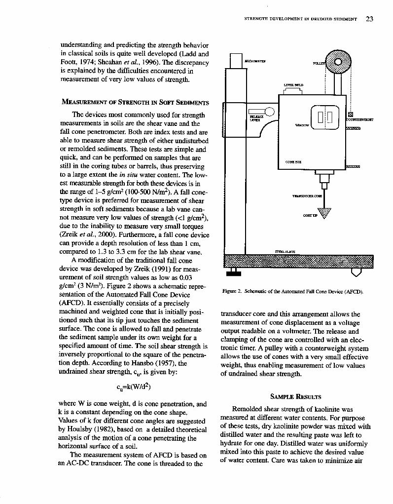
A modification of the traditional fall cone

device was developed by Zreik �991! for meas-urement of soil strength values as low as 0.03g/cm' � N/m'!. Figure 2 shows a schematic repre-sentation of the Automated Fall Cone Device

AFCD!. It essentially consists of a preciselymachined and weighted cone that is initially posi-tioned such that its tip just touches the sedimentsurface. The cone is allowed to fall and penetratethe sediment sample under its own weight for aspecified amount of time. The soil shear strength isinversely proportional to the square of the penetra-tion depth. According to Hansbo �957!, theundrained shear strength, c�, is given by:

where W is cone weight, d is cone penetration, andk is a constant depending on the cone shape.Values of' k for different cone angles are suggestedby Hobby �982!, based on a detailed theoreticalanalysis of the motion of a cone penetrating thehorizontal surface of a soil.

The measurement system of AFCD is based onan AC-DC transducer. The cone is threaded to the

STRENGTE DEVELOPMENT IN DREDGED SEDIMENT 23

Figure 2. Schemabc of the Automated Fall Cone Device AFCD!.

transducer core and this arrangement allows themeasurement of cone displacement as a voltageoutput readable on a voltmeter. The release andclamping of the cone are controlled with an elec-tronic timer, A pulley with a counterweight systemallows the use of cones with a very small effectiveweight, thus enabling measurement of low valuesof undrained shear strength.

Remolded shear strength of kaolinite wasmeasured at dif'ferent water contents. For purposeof these tests, dry kaolinite powder was mixed withdistilled water and the resulting paste was left tohydrate for one day. Distilled water was tuiiformlymixed into this paste to achieve the desired valueof water content. Care was taken to minimize air

24 PAHUtA ET AL

15

t5 io

5

ACKNOWLEDCEMENTS

LITERATURE CITEIJ

0 50 100 150 200 250 300 350Water Content %!

Figure 3. Variation in undrained shear strength of remolded kaolinitewith water content.

entrapment during Inixing.Six to eight strength measurements were taken

with the AFCD for each value of kaolinite water

content. The average values of tmdrained shearstrength are presented in Figure 3. The error barsenclose the interval of one standard deviation on

each side of the mean value of the measurements.

The figure also shows the results obtained by Zreik�994! on the same material, The resulting compar-ison indicates excellent repeatability of AFCDmeasurements.

Strength measurements were also performed onthe sediment retrieved from Reserved Channel in

Boston Harbor, a site that was dredged under theBoston Harbor Navigation Improvement Program BHNIP!. This sediment was homogenized andcharacterized prior to testing, Table 1 shows theremolded shear strength of Reserved Channel sedi-lnent at three different water contents.

These measurements adequately demonstratethe reliability of the Automated Fall Cone Devicein measuring very low values of undrained shearstrength of sediments. This capability is the basisof an experimental research program currentlyunderway at the MIT Geotechnical Laboratory,with the objective of understanding the process ofstrength development in consolidating dredgedmaterials. Specifically, it aims to ascertain therelative contributions of effective stress and

thixotropic strength gain to the total undrained

Table 1. Variation of undramed shear strength of remolded kaolinitewith water content.

shear strength. This understanding will provide thecrucial input for modeling of strength developmentin consolidating dredged sediments.

The authors are grateful to Dr. ThomasFredette of the U.S, Army Corps of Engineers New England Division! for his support. Additionalsupport was provided by the MIT Sea Grant CollegeProgram contract no: NA86RGO074! and the NewEngland Division of the U.S. Arlny Corps ofEngineers, through SAIC contract no: 4400039096!.

ENSR. 1997. Sronmary Report of Independent Observations, Phase I,Boston Harbor !Vavigation Improvement Project. ENSR Doc. No,4479-001-150, prepared for Massachusetts Coastal ZoneManagement, ENSR, Acton, MA.

Hansbo, S. 1957. A new approach to the determination of the shearsuength of clay by the fall cone test. Royal SwedishGeotechnical Institute, Stockhobn. No. 14.

Houlsby, GT. 1982, Theoretical analysis of the fall cone test.Geotechnique 32�!:111-118.

Ladd, C.C. and R. Foatt. 1974. New design pracedure for stability ofsoft clays. Journal of Geotechnical Engineering 100�!:763-786.

Lambe, T.W. and R.V. Whitman. 1969. Soil Mechanics. John Wileyand Sans. New York,

Mitchell, J.K. 1960. Fundamental aspects of thixotropy in soils.Journal of the Soil Mechanics and Foundations Division.ASCE. 8886 SM3!: 19-52,

SAIC Science Applications International Corporation!. 1997. Postcap Monitoring of Boston Harbor IVavigation ImprovementProject BLIP! Phase L Assessment of Inner Confluence CADCelL SAIC Report No. 413, prepared for the New EnglandDivision of the U.S. Army Corps of Engineers, Waltham, MA.

Sheahan, T.C., C.C. Ladd and J.T. Germaine. 1996. Ratt. dependentundrained shear behavior of ~ clay. Journal ofGeotechnical Engineering. 122�!:99-108.

Zreik, D.A. 1991. Determination of Undrained Shear Strength of VerySoft Cohesive Soils by a Ittew Fall Cone Apparatus. S,M.Thesis, Massachusetts Institute of Technology, Cambridge, MA.

Zreik, D.A. 1994. Behavior of Cohesive Soils and Their Drained,Undrained, and Erosional Strengths at Ultra-Low Stresses.Ph.D. Thesis, Massachusetts Institute of Technology,Cambridge, MA.

Zreik, D.A�C.C, Ladd and J.T. Germaiue. 2000. Discussion on yieldstress of super soft clays. Journal of Geotechnicai andGeoenvironmental Engineering, 126 8!:754-756,

PROPWASH MODELING FOR CAD DESIGN 25

Propwash Modeling for CAD Design

VLADIMIR SHEPSIS

DAVID P. SIMPSON

Pacific International Engineering PLLC123 Second Ave. South

Edmonds, WA 98020 USA

ABSTRACT: A numerical model has been developed fo simulate near-bed velocitiesgenerated by ships' propulsion. The model incorporates theoretical descriptions of thegeometry and velocity structure in a inomentum jet Field measurement programs haverecently afforded the opportunity to validate the niodel. The inodel is a reliable tool forestunating the velocity at speciYied distances from the bottom. Its application is suitedfor determining potential for sediment suspension, and for design of a stable capoverlying erodible sediments.

Key words: propwash, CAD, bottom velocity, bottom scour, sediment suspension

INTRODUCTION

THEORETICAL BASIS OF MODEL

Cottesponding anthon telephone: 425-921-1703;fi: 425-744-1400; email: vtadimir@piengr.corn

Confined Aquatic Disposal CAD! sites areoften located in open water and are usually sub-jected to effects of passing deep draft vessels, tugs,and small craft. Evaluating the hydrodynamicforces on surface sediment and the sediment cap iscritical to CAD design. Integrity of the sedimentcap is essential to the success of a ConfinedAquatic Disposal site in preventing dispersal ofsediments contained within the CAD. The follow-

ing describes the development and application of anumerical tool for calculating near-bed velocitiesgenerated by a ship's propulsion and the resultingpotential for scour of bottom sediments.

A numerical model is required to investigatevessel effects for many applications. The JET-WASH model was developed to operate with inputof sediment and propulsion characteristics andwater depth, and to output velocity at a given dis-tance aft of the vessel and radially from the velocityjet centerline, or at a known distance above thebottom. Exainple applications of the model are toevaluate:

~ Potential for vessel operation to harin Inarineplants, such as eelgrass;

~ Suspension and transport of fine sedimentsthat would degrade nearshore habitat; and

~ Penetration of a sediment cap that is intendedto isolate the underlying material.

Increasing concerns about sediment quality inmarine industrial areas and habitat preservation forendangered fish species in Puget Sound Washington State! was the impetus for develop-ment and testing of a Inodel that could quantifyhydrodynainics and sediment transport in the abovelisted applications. The writers coded formulaspublished in the engineering literature into a calcu-lation model named JETWASH. Planning andenvironmental studies for maintenance activities bymarine carriers provided opportunities to makefield measurements that served to validate the JET-WASH model.

Researchers have advanced mathematical

descriptions of the velocity field generated by jetsdischarging into a fluid body and by propellersrotating in a fluid. Formulas developed byAlbertson et al. �948!, Liou and Herbich �976!,Blaauw �978!, Verhey �983!, Fuerher et al.�987! describe the velocities and geometry of theturbulent jet as it expands into a volume of water.The structure of the water velocity is describedmathematically in two zones Figure 1!. The initialvelocity is calculated Rom details of the propellerand persists in the zone directly behind the pro-

sHnpsts a sIMpsox

FIELD MEASUREMENTS

Flow establishment

v vo

Theoretical axis of jet

DATA COLLATION

peller. The core of initial velocity in this first zoneis unaffected by transfer of fluid momentum to thesurrounding water. Downstream from the firstzone, water velocity is developed through transferof momentum from the core of initial velocity tothe surrounding water The edge of the cone ofexpanding turbulence in this second zone experi-ences lower velocity than the centerline, and thecenterline velocity diminishes with increasing dis-tance from the source,

Figure 1. Geometry of initial velocity zone and momentum jetformed by the propulsion system.

C. 6,r <++ r <+> isr

OC G<Nominal Limits of --.~ C aC,Diffusion Region

Hydrodynamic research shows that the velocityrequired to move sediment particles in waterdepends on several parameters, Succinct combina-tions of the pertinent parameters are the Shield'sparameter a ratio of the threshold boundary shearstress to the immersed weight of a sediment parti-cle! and the boundary Reynolds number a ratio ofinertial forces to viscous forces acting on the parti-cle comprising the bottom!. Cheng and Chiew�999! developed relationships between these twoparameters for the case of suspended load. Theirresults yield the shear velocity corresponding to theinitiation of suspension of sediment particles hav-ing a given diameter. Flow causing suspension ofsediment particles initially at rest is termed thescouring velocity. The flow velocity at a selecteddistance above the sediment bed necessary to sus-pend a given size sediment in the flow is deter-mined from the critical shear velocity and theequation for the logarithmic velocity distribution ina fully turbulent, hydraulically rough boundarylayer Middleton and Southard 1984, p. 152!.Modeled or measured velocity can then be com-pared with the theoretical suspension velocity in the

absence of sediment concentration measurements!to determine if the threshold for suspension isexceeded in the particular conditions.

Research reported by Hamill �988! provides ameans of calculating scour depth in bottom sedi-ment by a propeller. Empirical relationships devel-oped by Hamill among initial velocity, propeller tipclearance above the bottom, duration of exposureto the propwash, propeller diameter, and sedimentsize were formulated to calculate the maximumscour depth,

A coefficient describes the spread of themomentum jet in the fluid, or the angle of the edgeof the jet with respect to the centerline. The coeffi-cient has been evaluated by several researcherswith laboratory and limited field studies. PacificInternational Engineering conducted field data col-lection to validate the model with measured veloci-

ties and known propulsion characteristics.

Velocities were measmed at the bottom with an

Acoustic Doppler Velocimeter ADV!, whichrelayed data through a cable to a computer aboarda small survey boat anchored nearby. Figure 2shows the weighted instrument frame on which ismounted an ADV, a video camera, and compass.Figure 3 shows one measurement site marked withbuoys. A Global Position System GPS! unit wasmounted on board the test boat above the propelleror jet pump nozzle for recording position. The testboat position data were time stamped as they were

Figure 2. Velocity meter mounted on frame and suspended hornboat davit before deployment on the bottom!.

ae'llR.

ae

DATA PROCESSING

MODEL VERIFICATION

Figure 3. Test area marked with buoys and survey boat at anchor.

recorded on a computer aboard the test boat. Thecaptain was chrected to move the boat directly overthe velocity meter during the tests. The goal wasto capture the direct flow of the velocity jet as fullyas possible. As a test run began, the start time andmaneuver to be simulated were commtmicated

between the survey boat and the test boat by radio.Engine rpm was monitored in the wheelhouse ofthe test boat and manually entered on the computerthat recorded the GPS signal. The velocity wasmeasured 25 cm above the bottom. The horizontal

and vertical components of velocity were sampledat 0.04-second intervals. Velocity data were record-ed through a cable on the stuvey boat computer,which was also synchronized with the GPS signal.

The horizontal and vertical components ofmeasured speed were combined, resulting in a timeseries of speed for each test, The peak bottomvelocity is of interest because that is the quantitythat is most critical to determine the potential f' orscotUing of bottom sediments, The velocitiesdetermined at 0.04-second intervals were convertedto a 1-second-average velocity time series. Theduration of the period of high velocity indicates thelength of time during a particular maneuver thatpotential bottom-scouring conditions could persistif a threshold velocity was exceeded. Synchronousboat position, engine speed, and bottom velocitydata reveal conditions under which a particularvelocity pattern is generated. One example of avelocity time series is shown in Figure 4.

Boat and propulsion characteristics and siteconditions were input to the JETWASH model.Model output is summarized as a graph of velocity

PROPWASH MODELING FOR CAD DESIGN 27

e ee ee ee ee 1%t Wee lee lee lee eeeElapsed Time seconds!

Figure 4. Measured velocity time series for test vessel.

Figure 5. Predicted bottom velocity for test vessel.

at a distance of 0.83 ft �5 cm! above the bottomthat would be experienced at given distancesbehind the boat. The coefficient that describes theexpansion rate of the momentum jet was deter-mined to be 0.3 using velocity measurements of apair of ADVs separated by 12.5 ft �,8 m! mountedon a vertical. Separate velocity measurements,made 0.83 ft �5 cm! above the bottom, were usedfor model verification. Figure 5 is a graph of sim-ulated velocities for the conditions represented inFigure 4. The measured peak near-bottom veloci-ty indicated in Figure 4 is 1.1 feet per second �3.5cm per sec!. The simulated peak near-bottomvelocity indicated in Figure 5 is 1,05 feet per sec-ond �2 cm per sec!, Other runs involving bothpropeller- and jet pump-powered vessels were sim-ulated. The average velocity agreement, expressedby measured minus modeled as a fraction ofmeasured velocity, is � 0.1, which is judged to be

28 sBKPsls a sIMPsoN

SUMMARY

LITERATURE CITED

APPLICATION

good agreement.The underwater video did not indicate signifi-

cant sediment disturbance, although that providesonly a qualitative evaluation at best of the sedimentsuspension calculations. The velocity necessary tosuspend sediment of a given size was calculated asdescribed above for the test conditions, Results are

listed in the table below. The measured and rnod-

eled velocities do not exceed the velocity for sus-pension of bottom sediments of the sizes down tovery fine sand. The comparison confirms at leastqualitatively that the simulated velocity magnitudeand the procedure for estimating suspension of bot-tom sediments by near-bottom velocities generatedby vessel propulsion are correct for this type ofapplication.

Table 1. Velocity to suspend sediment of given size.

*Reference height is 0.83 ft above bottomSimulated conditions are Puget Sound water

The JETWASH model has been applied at sev-eral locations for purposes of design and environ-mental effects investigations. Example applica-tions in Puget Sound are:~ Colman Dock Resuspension Study�

Investigated potential for resuspension of con-taminated bottom sediments near a ferry dock.

~ Vashon Island Eelgrass Disturbance Study�Investigated the conditions under which ferryoperations would dislodge eelgrass from thebottom.

~ Southworth and Kingston Ferry Terminals-Investigated bottom scour and transport of finesediments onto eelgrass beds in the vicinity ofproposed ferry docks.

~ Foss and Hylebos Waterways � Aided in design

of sediment caps to confine contaminated sedi-ments in a deep-draft waterway.

~ Mukilteo Passenger-Only Ferry � Aided inselection of vessel for temporary use as ferrythat would not cause disturbance of bottom

sediments.

A numerical model was developed and verifiedfor simulating the velocity pattern in a jet createdby a ship's propulsion system. A calculation pro-cedure was developed for determining the thresh-old size of sediment suspended in a specified flowfield. Observation of the bottom showed the sedi-

ment suspension calculation procedure is acctnatein predicting sub-threshold conditions. Ftntherresearch can confirm the accuracy in scouringconditions.

Albertson, M.L., Y.B. Dai, R.A. Jensen, and H. Rouse. 1948.Diffusion of Submerged Jets, Transactions of the AmericanSociety of Civil Engineers, Paper No. 2409, 639 � 697.

Blaauw, H.G aud E.J. van de Kaa 1978. Emsion of Bottom andSloping Banks Caused by the Screw-Race of Manoeuvring Ships.International Harbour Congress. Antwerp, Belgium.

Cheng, Nian-Sheng and Yee-Meng Chiew, 1999, Analysis of initia-tion of sediment suspension from bed load. Journal of HydraulicEngineering. American Society of Civil Engineers. 125:8.855-861,

Fuehrer, M., H. Pohl, and K. Roemisch. 1987. Propeller jet erosionand stability criteria for bottom pmtections of various construc-tions, Bulletin of the P.I A.XC. No. 58. 45-56.

Hamill, GA. 1988. The scouring action of the propeller jet producedby a slowly manoeuvring ship. Bulletin of the P.I A.N.C. No. 62.85-110.

Liou, Yi-Chung and John B. Herbich. 1976. Sediment movementinduced by ships in restricted waterways. COE Report No, 188,TAMU-SG-76-209. College Station, TX.

Middleton, G and J. Southard. 1984. Mechanics of sediment move-ment. S.EP.M, Short Course Number 3, Second Edition. Societyof Economic and Paleontologic Mineralogists, Tulsa, OK.

Verhey, K J. 1983. The stabiTity of bottom and banks subjected to thevelocities in the propeller jet behind ships. In Proceedings of the8th International Harbour Congress. Antwerp, Beigium. June13-17,