conduct estimation via ownership · pdf fileconduct estimation via ownership change...
TRANSCRIPT

Conduct Estimation via Ownership ChangePreliminary Draft
Christian Michel∗
August 10, 2012
Abstract
This paper proposes a new form of estimating industry conduct in differentiated product in-
dustries. As an identification strategy, I use the structural ownership changes that occur due to
a merger. Given both pre-merger and post-merger industry data, I look for the form of conduct
that best predicts the market outcome before and after the merger. I provide identification results
for a new form of direct industry conduct estimation. Using both pre- and post-merger data also
enables me to provide a new evaluation criterion when selecting the form of competition among
a discrete “menu” of outcomes. I estimate industry conduct using data around a merger from
the Ready-to-Eat (RTE) cereal industry. Depending on the specification, I find that between
8.0% and 31.7% of industry markups can be attributed to cooperative industry behaviour, while
the rest of the markup is due to product differentiation of multi-product firms. My approach
also allows me to estimate the degree of profit internalization between merging firms post-merger
conditional on a specific form of competition. Furthermore, I provide ways to directly estimate
synergies resulting from a merger.
Keywords: Conduct Estimation, Identification of Market Structure, Ex-post Merger Evaluation,
Profit Internalization, Estimation of Synergies
JEL Classification: L11 (Production, Pricing, and Market Structure), L16 (Industrial Structure
and Structural Change), C52 (Model Evaluation, Validation, and Selection)
∗Graduate School of Economics and Social Sciences, University of Mannheim; Email: [email protected] am grateful to my advisors Volker Nocke and Philipp Schmidt-Dengler for their support throughout the project. I also wouldlike to thank Steve Berry, Pierre Dubois, David Genesove, Alex Shcherbakov, Andre Stenzel, Andrew Sweeting, Yuya Takahashi,Otto Toivanen, and seminar participants at Mannheim and Toulouse, as well as participants of the 2012 CEPR Applied IOSummer School for helpful comments. I am furthermore grateful to the Kilts Center of Marketing at the Graduate School ofBusiness, University of Chicago, for the Dominicks Finer Foods data.
1

1 Introduction
One of the key questions in industrial organization is which factors are the key determi-
nants for prices in specific industries. Such factors can be production costs, the degree of
product differentiation, and the form of market competition. Modern empirical research
in industrial organization often involves a detailed industry demand model, combined with
a game-theoretic formalization of supply side behavior. Very often, the form of supply side
competition is imposed by assumption rather than being tested for. This can be problematic:
If the imposed supply side specification turns out to be wrong, impacts of structural changes
in an industry, for example mergers or product entry, are likely to be mispredicted. The
main challenge is to jointly identify marginal costs and industry conduct in a differentiated
product model.
In this paper, I propose a new approach of estimating conduct in differentiated product
markets by using both pre-merger and post-merger industry data. My identification strategy
searches for the form of supply side competition that best predicts both pre-merger and post-
merger industry behavior. The intuition is the following. Given a well-specified demand-side
estimation and valid instruments, one can consistently estimate consumer price elasticities
irrespective of supply-side behavior. As is common in the literature, I assume that marginal
costs in the market are not observed by the researcher. Hence, different game-theoretic
assumptions about the competition in the market yield different estimates for marginal costs.
I make the common assumption that merging firms internalize the profits after the merger.
Given marginal cost estimates and the price-elasticities obtained from the demand side-
estimation, I can predict the effects of an ownership change on prices ex-post. By varying
the form of supply side competition (i.e. industry conduct), and accounting for input price
changes on the cost side, I look for the form of competition that most accurately predicts
the effects of the merger-induced ownership change on prices. I estimate the predicted post-
merger prices using only pre-merger data and compare them with the actual post-merger
prices. The differences of actual prices and predicted prices I then use to form moments in
order to obtain the model’s underlying conduct parameters using a Generalized Methods of
Moments estimation. I use data from the RTE cereal industry around a merger to test my
proposed method. In November 1992, Philip Morris with its Post cereal line purchased the
Nabisco ready to eat cereal branch. The antitrust court decision to clear the merger relied
heavily on empirical analysis, see for example Rubinfeld (2000) for a detailed analysis.
My approach has several advantages over the existing literature. I show that using proper
supply side variation, it is indeed possible to estimate industry conduct directly in differen-
tiated product models. This is something that is very unlikely to be achieved using demand
side variation, see for example Nevo (1998). I set up conduct moment conditions that rely
on orthogonality conditions between predicted price residuals and the true underlying form
of industry conduct. This helps me to overcome the problem of correctly estimating the un-
derlying level conduct parameters, instead of estimating only the responsiveness of industry
2

conduct with respect to cost variation. Moreover, my framework enables me to approach
various merger related supply-side issues. To my knowledge, this is the first paper to focus
on estimating post-merger intra-firm conduct of a merged entity, as well as to propose a
method to estimate merger related cost synergies directly in differentiated product models.
Advances in game theory, computational power, as well as econometric techniques have
lead to structural models that are able to recover the empirical counterparts to the theoretical
models. This has lead to a plethora of applications with respect to estimating demand or
production functions. While estimating industry conduct played a big role in the beginning
of the structural evolution, not much progress has been made over the past 15 years. Several
reasons contribute to this. Historically, conduct estimation has been closely related to the
concept of conjectural variations.1 Previous attempts to estimate both marginal costs and
industry conduct have mostly been made using demand side variation. In differentiated
product models these approaches usually face two kind of problems. The first problem is
the difficulty to find a sufficient number of demand rotators when estimating conduct in
differentiated product markets. Without such rotators, these approaches are not able to
identify industry conduct.2 The second problem relates to the estimation techniques, which
only estimate the economic parameters of interest accurately in special cases, see Corts
(1999). Corts critically discusses the identification of conjectural variation parameters.3 His
critique is twofold. Firstly, he argues that conjectural variation parameters usually differ from
the “as-if conduct parameters” one is interested in. A conjectural variation parameter only
estimates the marginal responsiveness of the marginal cost function with respect to changes
in a demand shifter. As a researcher, one is however interested in the average slope of the
marginal cost function instead of the marginal slope.
My approach differs significantly from the conjectural variations approach and is not sub-
ject to this critique. In my framework, each firm sets prices for its portfolio of brands instead
of quantities. Furthermore, instead of forming conjectures about other brands’ reactions,
each firm has an underlying objective function that takes into account preferences for profits
of other firms, thus allowing for cooperation among different firms. The preference parame-
ters with respect to other firms’ profits are essentially the conduct parameters I am interested
in. I assume that these conduct parameters, as well as the marginal costs of all brands, are
common knowledge in the industry, but not observed by the researcher. Using first order
conditions of all brands’ objective functions, my identification strategy then allows to esti-
mate both marginal cost parameters and the level conduct parameters, which amount to the
“as-if conduct parameters” in Corts (1999).
1Using a Cournot-style setting, one was able to derive equations from which conjectural variation parameters as a form ofresponsiveness towards industry competitors could be estimated, see for example Bresnahan (1989). In these models, a firmforms a “conjecture” about the responses of their competitors towards an increase in its own quantity. A conjecture can be seenas a reduced-form game theoretic best response function in symmetric quantity setting games. Conjectural variation modelsusually neglect any higher order effects of the best response functions. When accounting for higher-order rationality in the bestresponse correspondences, one can however show that only Cournot competition itself survives iterated deletion of dominatedstrategies.
2See for example Nevo (1998)3While his critique addresses homogeneous product models, his arguments are also valid for differentiated product models.
3

Corts second critique is related to the static game character of most conduct estimation
models. My approach is not fully exempt from this critique. I account for some industry
dynamics by modeling the merger-induced industry change. Nonetheless, it may be that my
static approach does not detect certain dynamic collusion patterns. One big advantage of
a static approach is a higher degree of tractability. Modeling repeated games makes identi-
fication of conduct even more difficult due to a multitude of potential dynamic equilibrium
strategies. With my approach, I am also able to identify patterns of full collusion as well as
patterns of collusion between only a subset of firms.
Related literature In this paper, I estimate conduct in differentiated product markets using
supply-side driven variation. Up until now the work in this area is relatively sparse, and
exclusively covers the airline industry. Oliveira (2011) uses marginal profit ratios in a dynamic
model to distinguish between market competition and efficient “stick-and-carrot” collusion
in the airline market. Orcholski (2010) sets up profit equations in a reduced form model and
backs out conjectural variation parameters that distinguish between Cournot-competition
and collusion. Ciliberto and Williams (2010), develop an approach that relies on multi-
market contact for estimating conduct in the the airline industry. Their model includes
conduct parameters that can have three different values, accounting for different degrees of
cooperation among profit-maximizing firms. In a differentiated demand model, Bresnahan
(1987) tests the hypothesis of a change in supply side competition in the US car market from
collusive to competitive against other options. Feenstra and Levinsohn (1995) formalize an
oligopoly setting which allows to estimate conduct in differentiated product industries for
different non-nested oligopoly models.
Bresnahan (1982) and Lau (1982) provide identification results for estimating conduct in
the homogeneous good case. Lau finds that if the inverse demand function is not separable
in the demand shifters, i.e. if it rotates rather than shifts due to demand shocks, then an
oligopoly solution is identified. Genesove and Mullin (1998) compare predictions from a
homogeneous good conduct estimation in the sugar industry with results from a direct cost
estimation. They find that a model with a freely estimated conduct parameter yields more
accurate cost estimates than estimates obtained from pre-specified models.
Nevo (2000) and Nevo (2001) use a random coefficient logit demand estimation to estimate
marginal costs and market power in the RTE cereal industry, and to predict effects of a merger
using only pre-merger data, respectively. Nevo (1998) theoretically discusses advantages and
disadvantages of a direct conduct estimation compared to a non-nested menu approach.
He argues that in practice estimating conduct directly will be impossible due to a lack of
sufficiently many distinct demand shifters. Hence, testing different non-nested models and
choosing the best fit for the data often seems to be the only viable alternative. For such non-
nested tests Vuong (1989) derives asymptotic results using a likelihood ratio test foundation.
Rivers and Vuong (2002) derive results on a more general basis. Gasmi, Laffont, and Vuong
(1992) further provide likelihood ratio tests for different oligopoly specifications in the soft
4

drink industry.
This paper is also related to other open questions in the field of industrial organization,
outlined in the following.
Ex-post evaluation of mergers One important question is how well different demand-side
models are capable of accurately predicting effects of mergers. Over the last decade, merger
simulations have become a regularly-used tool in antitrust cases. However, different demand
side models, such as logit, nested logit, or the Almost Ideal Demand Model will lead to
different estimates for price-elasticities, and therefore also different inferred marginal costs.
So far there is only a small number of papers exploring these issues, see for example Weinberg
and Hosken (2009) and Yoshimoto (2011). Not surprisingly, these models find that more
sophisticated estimation techniques, such as the Random-coefficient Logit model, yield more
accurate results than less sophisticated approaches such as the IV Logit model. Whereas
these papers test different demand side specifications, they ignore differences resulting from
supply side effects.
Estimating profit internalization of merging firms Different economic theories predict dif-
ferent degrees of post-merger profit internalization. From a neoclassical viewpoint, thus
neglecting agency problems within a firm, it makes sense to maximize joint profits of all
brands of the same firm. This is most important if a company has several brands that are
relatively close substitutes for consumers. However, there might be delays in post-merger
harmonization of firm strategies due to old contractual agreements and incentive structures.
Furthermore, from a theory of the firm point of view, it is possible that the different branches
remain different profit centers and thus compete within the firm. With my framework, I am
able to estimate intra-firm conduct conditional on a specific form of industry competition.
Direct estimation of synergies I use the availability of pre-and post-merger data to propose
a method to directly estimate synergies for merging firms resulting from a merger conditional
on a specific form of conduct. Examples for synergies are economies of scale or more efficient
production. Such synergies are often cited as a reason for allowing a merger that significantly
increases market power of merging firms. However, without having post-merger data it is
impossible to estimate synergies.
Selection methods – “menu approach” My baseline approach reflects the case in which I
estimate the conduct parameters and the marginal cost parameters directly using a moment
estimator. The advantage of this approach is that the possible values of the conduct parame-
ters are unconstrained, thus yielding a high degree of flexibility for the researcher. The menu
approach on the other hand selects the best fit among a discrete set (“menu”) of supply side
models, for example multi-brand Bertrand-Nash competition or a single profit-maximizing
5

monopolist. One advantage of this approach is that it does not include any conduct param-
eters directly, but rather pre-imposes them. Hence, there are less parameters to estimate
which often relaxes identification problems. There are two popular ways to select among
different non-nested models. However, both methods have significant weaknesses.
The first method relies on non-nested tests that only use pre-merger data, such as Vuong
(1989) or Rivers and Vuong (2002). These tests are based on a Kullbach-Leibler measure, and
test how far away a non-nested model is from the true data generating process pre-merger.
However, these tests tend to have relatively low predictive power. The second method relies
on recovering marginal cost estimates for different supply specifications, and comparing them
to accounting data. Such accounting data is problematic for various reasons. Firstly, the
data does not accurately reflect economic marginal costs. Secondly, these costs are usually
only available on an aggregate level. Therefore, it is very difficult to use these approaches
to test for some more advanced patterns of cooperative behavior, such as collusion among a
subset of firms.
My test is based on the fit of the data pre-merger and post-merger, and I exploit changes
in ownership as well as variation in the input cost data to select among different non-nested
models.
In the following, I will at first focus on the model setup and on identification issues regarding
the estimation of industry conduct. Section 2 introduces the baseline model and discusses
the conduct estimation strategy in detail. Section 3 will provide identification results to
estimate conduct and marginal costs jointly. Section 4 presents the data and estimation
results. Section 5 introduces several extensions to the baseline model as outlined above.
Section 6 concludes with a discussion of both the results and some open questions.
2 Empirical Model
My framework relies on two basic steps. In the first step, I estimate industry demand using a
discrete choice model to back out price elasticities. In a second step I then estimate industry
conduct either using a direct conduct estimation routine or using a menu approach. Both
approaches rely on forecasting post-merger prices giving pre-merger data and then to compare
them with the actual post-merger prices. In the second step I will also be able to compute
price-cost margins of the different products and to estimate the influences of different input
prices on marginal costs.
2.1 Demand side
My demand specification is closely related to Nevo (2001). There is a total number of J
brands in the market.
Denote the number of individual consumers in every market by I, and denote the number
of time periods by T . Using a Random Coefficient Logit model, individual i’s indirect utility
6

of consuming product j at time t can be written as
uijt = xjtβi + αipjt + ξjt + εijt; (1)
i = 1, .., I; j = 1, .., J ; t = 1, .., T .
xjt denotes firm j’s observable brand characteristics, pj denotes the price of product j, and
ξjt brand-specific mean valuation that is unobservable to the researcher but observable to the
firms. In some specifications I will decompose the brand-specific unobservable component
into several parts: ξjt = ξj + ξt + ∆ξjt. In this case, ξj denotes a mean unobservable brand-
valuation across all stores, ξt denotes a time-trend across all brands, while ∆ξjt is a store
and time specific component that is treated as an error term.4 Finally, εijt is an idiosyncratic
error term. The coefficients β and α are indiviual specific coefficients. These coefficients
depend on their mean valuations, on demographics in each region, Di and their associated
coefficients Π, as well as on an unobserved vector of shocks, vi that is interacted with a
scaling matrix Σ:(αi
βi
)=
(α
β
)+ ΠDi + Σvi, vi ∼ N(0, IK+1). (2)
Because not all of the potential consumers purchase a good in each period, I also require
an outside good. The indirect utility of the not purchasing any product and thus consuming
the outside good can be written as
ui0t = ξ0 + π0Di + σ0vi0 + εi0t.
As is common in the literature, I normalize ξ0 to zero.
Denote γD the vector of all demand side parameters. This vector can be decomposed
into a vector of linear parameters, γD1 = (α, β), and a vector of nonlinear parameters γD2 =
(vec(Π), vec(Σ)), respectively.
The indirect utility of consuming a product can be decomposed into a mean utility part
δjt and a mean-zero random component µijt+εijt that takes into account hetereogeneity from
demographics and captures other shocks. The decomposed indirect utility can be expressed
as
uijt = δjt(xj, pjt, ξjt, γD1 ) + µijt(xj, pjt, vi, Di; γ
D2 )
δjt = xjβ − αpjt + ξjt, µijt = [pjt, xj]′ ∗ (ΠDi + Σvi), (3)
where [pjt, xj] is a (K + 1)× 1 vector.
Consumers either buy one unit of a single product or take the outside good. They will
choose the option which yields the highest indirect utility. Using these assumptions, this
4The time trend ξt is not present in Nevo (2001). Since I use pre-and post-merger data for my demand-side estimation, usingsuch a time trend for post-merger data will increase my accuracy when relevant.
7

characterizes the set Ajt of unobservables that yield the highest utility for a specific choice j:
Ajt(x.t, p.t, ξ.t, γD2 ) = (Di, vi, εt)|uijt ≥ uilt∀l ∈ 0, .., J,
where dotted indices indicate vectors over all J brands. The market shares predicted by
the model can then be obtained via integrating over the different shocks, using population
moment functions P ∗():
sj(x.t, p.t, ξ.t, γD2 ) =
∫Ajt
dP ∗ε (ε)dP ∗v (v)dP ∗D(D). (4)
There are several possibilities to estimate the model that depend on different distribu-
tional assumptions. The most general case is a Random Coefficients Logit model. Its main
advantage is a very flexible form of substitution patterns. This is desirable because it enables
a detailed analysis of the substitution patterns between different brands that does not rely
on any model structure. To be able to integrate out the market shares, one needs to make
distributional assumptions with respect to the unobservable variables (Di, vi, εijt) and then
estimate the model using a GMM routine. Because of the non-linear aspect of the random
coefficients, such a model is relatively complicated and also computationally intense. As an
alternative, more rigid random utility models, such like Multinomial Logit model, can be
used. The main advantage is computational simplicity, for all heterogeneity is attributed to
an error term with known distribution. However, this also implies that substitution patterns
are proportional to market shares only, and not related to other factors like product charac-
teristics or brand proximity. As Nevo (2001) points out, this leads to a downward bias with
respect to the substitution to other inside goods.
When using a standard multinomial logit assumption, the error term follows an extreme
value distribution, i.e. the cumulative density function has the form F (ε) = exp(−exp(−ε)).
2.2 Industry technology
The J brands in the industry are produced by N ≤ J firms. Each brand can only be
produced by one firm. An important part of the model is the representation of marginal
cost. As is common in the literature, I assume that marginal costs can be decomposed
into cost factors that are observed to the researcher as well as factors unobserved to the
researcher. I allow for unobserved cost factors to be correlated with unobserved brand effects
and for observed cost factors to be correlated with observed brand characteristics x. I use
a linear relationship between marginal costs and the observable cost factors. This reflects a
relatively weak substitutability of input production factors over the medium- and short-run
in the RTE cereal industry. Denote the vector of brand j′s observed cost drivers by wj, and
j’s unobserved cost component by ωj. The marginal cost can be written as
mcj = wjγS + ωj (5)
8

where γS is a vector of marginal cost parameters. The estimated parameters will later be
used together with post-merger input cost data to predict post-merger marginal costs. The
baseline specification implies that marginal costs are constant for different output levels. This
is a relatively strict assumption, which can be relaxed by introducing scale effects. Denote
qi firm i′s total units sold in a period. If one assumes scale effects, i.e. decreasing marginal
costs in total production together with a Cobb-Douglas production function, then this can
be written as mcj = τ log(qj) + wjγS + ωj, where τ is the scale parameter.
2.3 Industry conduct
The key of this paper is to test for the form of competition in the market rather than to
pre-assume it. This is why I allow a firm’s objective function to potentially depend on other
firm’s profits. A firm can have a portfolio of different brands. Denote firm’s f portfolio by
Ff . Each brand maximizes its objective function with respect to its price. This can also
include profits of other firms’ brands. I make the assumption that all firms fully internalize
the profits of all the brands in their portfolio. Denote by θij the degree to which brand i takes
into account brand j’s profits when setting its optimal price, which reflects my interpretation
of a conduct parameter in my model. The conduct parameters are normalized to lie in
between 0 and 1. The assumption that each firm fully internalizes the profits of all of its
firms implies θii = 1∀i = 1, .., J , i.e. a brand fully cares about its own profits, and if i, j ∈ Ff ,θij = 1. Note that since only relative weights matter for the first order condition, this is a
normalization without loss of generality. Not allowing for negative conduct parameters also
implies that a firm does not derive a positive utility from “ruining” another firm.
The marginal costs of all brands in the industry are common knowledge as well as how each
brand takes into account all other brands. Both marginal costs and the conduct parameters
are however not observed by the econometrician. Brand j′s objective function can be written
as
Πj = (pj −mcj)sj +∑r 6=j
θjr(pr −mcr)sr, (6)
where sr denotes the market share of brand r.
Furthermore, the profit of all other brands enters the objective function additively. One
feature of such a framework is a linear structure that is easy to estimate. In any case, the
first order condition for brand j with respect to its own price can be written as
sj(p) +J∑r=1
θjr(pr −mcr)∂sr∂pj
= 0. (7)
Denote by Θ the pre-merger ownership matrix which can be defined as the matrix that
9

consists of entries
Θjr = θjr.
This leads to leads to
Θ =
1 θ12 .. θ1J
θ21 1 .. θ2J
.. .. .. ..
θJ1 θJ2 .. 1
The key of my estimation technique is to find the form of conduct and marginal costs
that best rationalizes pre-merger and post-merger prices. Since marginal costs conditional
on a specific form of conduct can be inferred using pre-merger data, I am interested in
recovering the matrix of conduct parameters Θ that best predicts these price changes with
respect to observed post-merger data. Because I assume that the merger-induced change in
conduct is known, the overall objective is to recover the pre-merger ownership conduct. As
a convention, the pre-merger ownership matrix does not contain a subscript “pre”. Define
Ωjr ≡ −θjr ∗ ∂sr∂pj
. When estimating the demand side using the pre merger data only and
being given proper demand side instruments, one can already infer the marginal costs of
production mc(γD,Θ,Ωpre(γD,Θ)) conditional on the form of conduct Θ.
mc(γD,Θ,Ωpre(γD,Θ)) = ppre − (Ωpre(γD,Θ))−1spre. (8)
Combining this equation with equation (5), one obtains the following expression for the
unobserved cost component ω given only pre-merger data:
ω = p− Ωpre(Θ, γD)−1spre − w′γS (9)
I treat product characteristics with respect to demand, x, and cost characteristics, w, as
exogenous with respect to industry prices. This is arguably a simplification in the long run,
but will facilitate the computation of the model.5
Objective Function Taken a specific conduct matrix Θ as given, in combination with the
parameters γD from the demand side estimation, all parameters necessary to recover pre-
merger marginal costs and to estimate equation (5) are given. The change in ownership due to
the merger also has an effect on pricing. A key identifying assumption is that even though the
researcher does not know the underlying form of conduct, Θ, he knows exactly how the merger
will affect industry conduct. There are two channels for this, namely post-merger profit
internalization of merging firms, and how competitors consider the merged entity post-merger.
5One short run effect that might be overlooked is how add-on toys in kids cereal boxes is affected by competitors’ prices. There is however anecdotal evidence with respect to collusive agreements regarding limits for kids toys in the RTE cerealindustry, see Corts (1995).
10

I will elaborate on the second channel in detail in section 3.1. Given the underlying form
of pre-merger conduct, Θ, the post-merger conduct can then be expressed as via a function
b : Θ→ Θ which maps the pre-merger conduct matrix Θ into the post-merger conduct matrix
Θpost = b(Θ). This is because all merger-induced ownership transformations are known by
assumption. This then allows to compute the post-merger markup Ωpost((γD, b(Θ)))−1s,
where Ωpost is the markup matrix which depends on the demand elasticities and the form or
post-merger conduct b(Θ). The predicted post-merger prices given γD for a specific Θ can
be written as
ppost(γD, γS,Ωpre(γD,Θ),Ωpost(γD, b(Θ))) = mc(Ωpre(γD,Θ), γS)−(Ωpost(γD, b(Θ)))−1s. (10)
mc(Ωpre(γD,Θ), γS) reflects the predicted marginal costs using the observed pre-merger
cost parameters γS together with the post-merger input prices. I use the predicted prices
conditional on industry conduct to form moment conditions that enable the identification of
the conduct parameters. Overall, I am interested in the matrix Θ among all potential supply
sides that minimizes a weighted moment criterion explained in the next two sections.The
next section discusses the differences of these options in more detail, and presents some
identification results.
3 Identification
The key identification question is: Under what circumstances are firms’ marginal costs and
industry conduct jointly identified? One important point with respect to marginal costs is
whether a merger will lead to synergies for the merging firms. In the baseline case I implicitly
assume that a merger will either not lead to synergies or involve a known synergy level in
form of a certain percentage decrease in marginal costs. The latter case enables, for example,
to account for synergies that are claimed by merging parties prior to a merger. This is also a
standard convention in merger simulation models. In this section, I will present identification
results for the direct approach. Section 3.1 introduces further assumptions to decrease the
parameters space to meet necessary rank conditions. Section 3.2 discusses the identification
assumptions for estimating both the demand and supply side parameters of the model.
3.1 Rank Conditions
3.1.1 Direct approach
This section provides identification results for different specifications when estimating con-
tinuous conduct parameters “directly”. This is opposed to the menu approach, which selects
among different non-nested models without estimating conduct parameters. Recall the as-
sumptions made on firms’ own-profit maximization. As in standard unilateral merger models,
I also assume that a merger does not change the behavior between non-merging firms. There
11

are furthermore some global assumptions that further reduce the parameter space which I
will discuss in detail.
I only consider cases in which a firm treats all brands of a specific competitor’s firm in
the same way. This excludes the possibility that single brands of different firms collude
while others play against each other competitively. There are two reasons for this. Firstly,
from a pure rank condition perspective the number of parameters I would have to estimate
would easily exceed the number brands in the market. This makes it impossible to identify
the parameters. Secondly, my demand estimation uses the brand space J as the limiting
distribution.
Conduct between merging and non-merging firms My identification strategy also requires to
specify how conduct will change between merging and non-merging firms after the merger
has taken place. Assume for example that there are 3 firms, 1, 2, and 3. Firm 1 and 2 will
merge. Before the merger, firm 3 could potentially have had a different relationship towards
firm 1 than towards firm 2. Thus, in order to identify the conduct parameters, I have to make
an additional assumption concerning how the two parts of the merged entity are considered
by their competitors after the merger. Any assumption that fulfills the property of a known
change in post-merger conduct is theoretically feasible. Analytically, this means that the
mapping b from pre-merger to post-merger conduct is known. I allow for three specific cases.
In the first case, the merger does not change how competitors consider the two merging firms
in the short run. In this case, while the merging firms will fully internalize the profits after
the merger, the rest of the conduct parameters will remain constant. A second possibility is
that the fully merged entity is considered and behaves as the acquirer did pre-merger. The
third option I allow is the reverse, meaning that the merged entity behaves as the target.
This is summed up in the following assumption.
Assumption 1 (Conduct between merging and non-merging firms). Let f, g be two distinct
merging firms, and h a non-merging firm. Let θpreik and θpostik denote the pre- and post-merger
conduct parameters between firms i and k, respectively. Then, ∀i ∈ Ff , ∀j ∈ Fg, ∀k ∈ Fh, one
of the following three cases holds regarding the conduct between a merging and a non-merging
firm:
a. θpostik = θpreik ; θpostjk = θprejk (no change in conduct);
b. Go to “acquiring firm” values: θpostik = θpreik ; θpostjk = θpreik (acquiring firm standard).
c. θpostik = θprejk ; θpostjk = θprejk (target firm standard);
It is worthwhile discussing the implications of this assumption. I do not have to pre-
specify the values of the conduct parameters, but just the way in which the parameters
change. As long as the change in conduct between merging and non-merging firms is known
post-merger, other change patterns are possible that still allow identification of the system.
An even stronger possibility is to assume specific values of the conduct parameters. In this
12

case, identification of industry conduct is also possible. This will be discussed in more detail
in section 5.
Bilateral symmetry between firms One way to reduce the number of parameters to be esti-
mated is to restrict the model to cases in which all brands of two firms play against each other
in the same way. As a consequence, all brands have the same cross-conduct parameters for
all of their brand pairs. This still allows for partial collusion between two firms, but does not
allow for more elaborate strategies, such as for example collusion only between some brands
of two firms. In terms of the parameter space, this reduces the number of cross-conduct
parameters to N(N−1)2
.
Proposition 1 (Necessary conditions for bilateral symmetry between firms). Suppose As-
sumption 1 holds, and that for distinct firms f, g , θij = θik = θji = θki ∀i ∈ Ff ,∀ j, k ∈ Fg.Then industry conduct is identified only if N(N−1)
2≤ J .
Proof. The demand parameters γD can be estimated from equations 10 and 13, respectively.
Regarding the supply side, there are J estimable equations, one equation per brand post-
merger. Because each firm has one conduct parameter for each competitor, this leads to an
overall number of N(N − 1) parameters. The bilateral symmetry assumption reduces this
number to N(N−1)2
. This leads to J equations with N(N−1)2
parameters. The model is only
identified if there are at least as many equations as parameters, i.e. if N(N−1)2
≤ J . This
completes the proof.
Same responsiveness to all cross-firm brands Another possibility is a case in which each firm
behaves in the same way to all of its competitors.
The advantage of this specification is that it reduces the number of parameters to only N
different cross-conduct parameters. However, there are also several problems associated with
the assumption. Firstly, it is again no longer possible to detect partial collusion between
a subset of firms in the industry. Secondly, there is a consistency problem with respect to
a mutual responsiveness: Under this assumption, it can be possible that firm 1 is acting
collusively with firm 2, and firm 2 on the other hand acts competitively towards firm 1,
something which is hard to justify from an economic perspective.
Proposition 2 (Necessary conditions for same responsiveness to all cross-firm brands). Sup-
pose Assumption 1 holds, and that for distinct firms f, g, h , θij = θik ∀i ∈ Ff ,∀ j ∈ Fg,∀ k ∈Fh. Then rank conditions are met only if N ≤ J .
Proof. The demand parameters γD can be estimated from equations 10 and 13, respectively.
Regarding the supply side, there are J estimable equations, one equation per brand pre-
merger, and one equation per brand post-merger.Because each firm has one conduct param-
eter for all firms, this leads to an overall number of N conduct parameters. This leads to
13

Conduct specification No or known synergies
Bilateral symm btw. firms N(N−1)2 ≤ J
Same resp. to cross-firm br. N ≤ JSame resp. btw. all firms J ≥ 1 (always met)Menu approach J ≥ 0 (always met)
Table 1: Identification conditions for different specifications
J equations with N parameters. The model is only identified if there are at least as many
equations as parameters, i.e. if N ≤ J . This completes the proof.
It is easy to see that the necessary rank conditions hold trivially. It can still be the
case however that there are two or more identical conduct equations, which would violate
identification.
Same responsiveness between all firms The most restrictive specification assumes that the
cross-conduct parameters are identical for all brands in the market. The biggest advantage is
that this returns a single cross-conduct parameter instead of a complicated matrix, and thus
always meets the rank conditions. The big disadvantages are that very often this parameter
will severely restricts the set estimable of economic models. For example, one will not be able
to test for partial collusion in the market, or for differences in competitive behavior between
different firms.
Proposition 3 (Necessary conditions for same responsiveness between all firms). Suppose
for distinct firms f, g, h , θij = θji = θik = θjk = θkj ∀i ∈ Ff ,∀ j ∈ Fg,∀ k ∈ Fh. Then the
rank condition for industry conduct is always met.
Proof. Using the same reasoning as in the proof for Proposition 2, there are J equations and
one parameter to estimate, so that the result trivially holds.
Overall, the direct approach requires more structure and a larger parameter space. This
is because the free-floating conduct parameters require more degrees of freedom. Therefore, I
will provide results specifically tailored for the different assumptions provided in the beginning
of this section. Clearly, the most important trade-off is the one between the allowed flexibility
of industry conduct and the number of parameters that have to be estimated.
3.1.2 Other forms of identification
Identifying conduct via product entry or exit Besides using a merger as an identification
strategy for estimating industry conduct, one can also think about using other structural
changes. Concerning product entry, there is the problem of comparing competition with and
without the entrant. While one can still make the assumption that entry does not change
how existing brands compete with each other, one has to define how a new product will
interact with the existing products. The menu approach is theoretically feasible under entry.
14

Unlike product entry, using product exit as an identification strategy is still feasible.
However, one has to ask why a product will exit. One reason can be that it is just not
profitable, which will then probably imply that its impact on the market is relatively low.
Therefore, a reduction of the brand space would not result in a big shift for firms strategies.
Another possibility would be that a brand is profitable on its own, but it would be more
profitable for a multi-brand firm to exit the product out of the market. This would result in
an endogeneity problem when estimating conduct using product exit.
3.2 Model identification
My estimation method requires identification of three sets of parameters: demand-side pa-
rameters, γD, cost parameters γS, and the conduct parameters Θ. The correlation between
price and both unobserved brand and cost characteristics requires instrumentation for each
brand in the demand and pricing equations, respectively.
3.2.1 Identification of demand parameters
Concerning the demand side, I assume that when being assessed at the true parameter values
γD0 , the unobservable demand components ξj for each brand are uncorrelated with respect to
a set of exogenous instruments, Zξ:
E[ξj(γD0 )|Zξ] = 0 (11)
Note that I implicitly assume that the demand estimation can be done independently of
the conduct and marginal cost estimation, respectively. The mean independence assumption
would be violated if industry conduct or a change in production costs, not prices, would
influence consumer choice through the unobserved brand-specific component.6 As common
in the literature, I assume that the product locations of the different goods is exogenous, and
therefore are does not respond changes in industry pricing or demand. Also accounting for
potential brand replacement or additional brand introductions would make traction of the full
model nearly impossible. Because of the inherent endogeneity between price and unobserved
brand characteristics, I need to find adequate instruments for the demand estimation. I use
four different sets of instruments to do so.
First-order basis functions of product characteristics The first set of instruments results from
setting up optimal instrument functions that result from the different product characteristics.
The economic intuition of these instruments is that product characteristics can influence
markups of the different products. A good with closer substitutes will have lower markups
than a less substitutable good. Furthermore, in a competitive oligopoly model, these markup
6This assumption would be violated if the merger caused a change in the perceived “brand values” of the merged entities,which would affect the ξ components in the demand equation.
15

effects will be even stronger for goods that have substitutes from other firms than from the
same firm. BLP (1995) argue that the computation of the optimal set of instruments when
only conditional moment conditions are available is very difficult and numerically complex.
As a less computationally demanding approximation, they use polynomials resulting from
first order basis functions of the product characteristics. The validity of these basis functions
as instruments relies on exchangeability assumptions of firms’ own characteristics with respect
to permutations in the order of competitors’ product characteristics. Because I allow for the
possibilty of collusion among firms, this changes the structure of potential Nash equilibria.
Cost shifters My second set of instruments relies on production cost shifters. The economic
assumption is that input cost variation should be correlated with variation in prices, but not
with consumers’ preferences for unobservable product characteristics. I use both cost factors
that affect all products in similar fashion, such as labor costs, packaging, and transporta-
tion, as well as factors that differ among products, such as interactions between product
characteristics and input prices for wheat, sugar, and corn.
Ownership change My third set of instruments is the ownership change itself. As argued
above, a merger should cause a change in industry prices. Similar to a cost shift, one can
assume that the merger affects prices, but not the demand characteristics. This assumption
would be violated if the merger caused a change in brand value which would affect the ξ’s of
the merging firms. Because the actual brand names of the cereals involved did not change
after the merger, such a brand effect seems unlikely.
Average prices in other zones A prominent set of instruments are prices from other pricing
zones, see for example Hausman (1996) and Nevo (2001). In my dataset, stores are located
in thirteen different zones within the same metropolitan area, and different zones are priced
differently. For validity of the instruments, the pricing decisions have to be uncorrelated
among different zones. Furthermore, demand shocks should not spill over across zones. Thus,
under the assumption that unobserved demand shocks are independent across clusters, prices
of other zones are valid instruments. This seems to be a very strong assumption in my dataset,
due to common advertising campaigns within the same metropolitan area and retailer. Still,
in non-sale periods, there are up to 20% price differences for the same product over different
stores.
3.2.2 Identification of cost parameters
Unlike the estimation of demand parameters, the estimation of both industry conduct and
cost estimates is unavoidably interlinked. In my approach, conditional on a specific form of
conduct, I can back out the marginal cost via a first order condition and then regress them
on observable product characteristics combined with input prices. This will then allow me
to predict the post merger marginal costs using post-merger input data and the estimated
16

parameters. My identifying assumption concerning marginal cost is that the unobserved cost
characteristics ω are mean independent to a set of exogenous cost instruments:
E[ωj(γS0 ,Θ, γ
D)|Zω] = 0 (12)
Note that in this stage, I do not use any information on conduct. This is because I use the
obtained cost parameters in order to forecast the marginal cost in the second stage. Together
with the change in ownership, this will influence the post-merger prices in the market. I will
then use both marginal cost and conduct effects in order to estimate industry conduct. I use
three different sets of instruments to identify the unobservable brand component.
First-order basis functions of cost characteristics Similar to the demand side estimation, I use
first-order basis function of the cost characteristics to instrument for the unobservable cost
component. The brand specific unobservable marginal cost component ω may be correlated
with unobservable product characteristics. Therefore it is essential to look for instruments
that are correlated with marginal costs, but not with the error term. To account for the
effects of unobserved cost drivers on prices, I use first order basis functions of the own
brand characteristics, own firm characteristics, and competitors’ characteristics. This again
relies on an exchangeability argument of product characteristics when facing a unique Nash
equilibrium, see for example Berry et al. (1995).
Retail margin In my data, I also observe a proxy for the retail margin, namely average
acquisition costs. This component is highly volatile over time. When not distinguishing
between the retail margin and the marginal cost of production in the estimation, but rather
treating both together as overall marginal cost, the data on the change in retail margin can
thus help me to identify the constant product-specific unobservable component ωj.
3.2.3 Identification of conduct parameters
To identify the conduct parameters, I use further orthogonality assumptions. Because I
assume that firms act according to my model and given a specific underlying form of conduct,
I can use the obtained predicted post-merger prices to generate two more sets of moments.
The first moment uses economic assumptions on the price effects within a single firm, whereas
the second one uses assumptions on prices between two different firms. As section 3.1 has
shown, the number of parameters varies with the conduct specification, between 1 and N(N−1)2
parameters.
Own firm conditions Denote df a dummy variable that equals one whenever a product
belongs to firm f and zero otherwise. The sum of the difference between predicted and
actual post-merger prices of a firms’ products should on average be uncorrelated to its own
dummy-variable df . This identification condition relies on the oligopoly structure of the
17

game. If the sum of the firm’s price residuals is on average correlated to this dummy, this
would imply that a firm is not pricing optimally given its preference structure, which is ruled
out by assumption. Therefore, a correlation between the firm’s dummy and the sum of its
own-residuals indicates a supply side misspecification to the researcher. Formally, define the
average squared price residual of firm f as
ϕownf (Θ, γS, γD) ≡ 1
TN
ST∑t=1
1
Jf
∑i∈Ff
(pposti,t (γD, γS,Ωpre(γD,Θ),Ωpost(γD, b(Θ)))−pposti,t )2. (13)
Here, Jf denotes the number of brands of firm f. Following the argument above, this leads
to the identification condition
E[ϕownf (Θ0, γS, γD)|df ] = 0 ∀i ∈ Ff∀j /∈ Ff , (14)
where Θ0 denotes the true vector of all conduct parameters. Overall, this will yield at
least N − 1 different moment conditions under Assumptions 1b and 1c. Under these two
assumptions, one conduct parameter will disappear post-merger. This will not be the case
under Assumption 1a. If one assumes the same behavior to all firms, then the involved
cross-conduct parameters θij turn to the single parameter θi. One can also use higher order
moments of the own-firm residuals to form even more moment conditions. As an alternative,
one can use assumption on the cross-conduct between two firms.
Cross-firm conditions Denote dfg a dummy variable that equals one whenever firms’ f and
g are interacting with respect to price setting, i.e. whenever firm f sets a price and takes
into the account the effects on firm g or vice versa. Given the true underlying supply side
model, the product of the average residuals between the predicted and actual post-merger
prices of two different firms should be mean independent of the underlying cross-conduct
parameter. The reasoning is similar to the one in case of own firm conditions: On average,
the price-residuals between two firms should not be correlated with the conduct parameters.
For notational simplicity, I now drop the expressions for pre- and post-merger markup,
Ωpre(γD,Θ), and Ωpost(γD, b(Θ)), respectively, from the equation for the predicted post-
merger prices. The average product of the squared price residuals between two firms f
and g can then be defined as
ϕcrossf,g (Θ, γS, γD) ≡ 1
TN
ST∑t=1
(1
Jf
∑i∈Ff
(pposti,t (γD, γS,Θ)−pposti,t )2)(1
Jg
∑j∈Fg
(ppostj,t (γD, γS,Θ)−ppostj,t )2).
(15)
From the above reasoning, one can now set up the following identification condition:
E[ϕcrossf,g (Θ0, γS, γD)|dfg] = 0 ∀i ∈ Ff , ∀j ∈ Fg. (16)
18

This yields at least (N−1)2
2and a maximum of N(N−1)
2different cross-firm moment con-
ditions. The number of cross-firm moment conditions depends on the selected assumption
regarding conduct between merged and non-merged firms. When adding up both cross-firm
and own-firm moment conditions, one obtains at least (N−1)(N+1)2
moments, which is sufficient
for estimating the N(N−1)2
parameters under bilateral firm symmetry.
Why has conduct to be known among firms? Suppose conduct where not known among
different firms. This would cause several problems. Firstly, this would make the assumption
on symmetry between two different firms harder to sustain. Secondly, I would have to specify
beliefs of the different firms regarding other firms’ behavior, which would further complicate
the model.
4 Data and Estimation
4.1 Industry Overview and Data
Industry description There are several factors that make the RTE cereal industry an ideal
starting point for oligopoly analysis.7 Economies of scale in packaging different cereals, as
well as in the distribution of products, cause barriers to entry for new firms. R&D expendi-
tures are relatively low, and only amount to 1% of gross sales per year. Still, there is a quite
frequent introduction of new products, which goes in line with large advertising campaigns in
the beginning of a product’s life.8 Market shares of successful brands over time are relatively
steady, which can easily be attributed to habit formation by consumers. The cereals differ
with respect to their product characteristics, such as sugar content or package design, and
target different audiences. It is common to classify these cereals into different groups, such as
adult, family, and kids cereals, see also Nevo (2001). Table 11 shows the classification of the
different cereal brands into different segments. At the start of the period I analyze , the in-
dustry consists of 6 main nationwide manufacturers: Kelloggs, General Mills, Post, Nabisco,
Quaker Oats, and Ralston Purina. See table 4 for the market shares of the different products.
Kelloggs as the firm with the biggest market share has a big presence in all segment. General
Mills is mainly present in the family and kids segments, whereas Post and Nabisco have their
main strengths in the adult segments. On a retail level, cereals are mostly distributed via su-
permarkets. Supermarket promotions via price reductions or quantity discounts are a further
tool used to increase quantities sold for a period of time. Furthermore, many retailers also
own private labels that compete locally with the nationwide manufacturers. I use scanner
data from January 1991 until May 1997 from the Dominick’s Finer Food database. Further-
more, I use input price data from the Thomson Reuters Datastream database over the same
7This industry has already been studied extensively, see for example Schmalensee (1978), Nevo (2000), and Corts (1995).Although Corts presents a detailed industry description, to my knowledge the dynamic aspects on the supply side have not beeninvestigated in detail.
8Hitsch (2006) studies the determinants of successful brand introductions. While I observe some product entry in the dataset,these products do not have a large share market share, such that I will leave them out in my main estimation.
19

time. My main dataset for the conduct estimation includes 28 brands from the 6 different
nationwide firms. The scanner data involves 68 stores from the Chicago Metropolitan area,
see Fig. 1 for a geographic map of the stores. In particular, the dataset includes data with
respect to product prices, quantities sold, data on promotions, as well as 1990 census data
yielding demographic variables for the different store locations. Even though I also observe
data on Dominick’s private label cereal, I do not include it in my conduct estimation. There
are two reasons for this. Firstly, I want to focus on the degree of competition between firms
that are operating nationwide. Because a private label is only present for one retailer, and
in my case a locally operating retailer, it will have different underlying objectives than the
nationwide operating manufacturers. Secondly, a private label firm belongs to its retailer,
thus leading to a joint maximization of profits upstream and downstream. This would need
more assumptions to be compatible with estimating “upstream ” industry conduct. I also
abstract from dynamic storage behavior, as well as couponing and shelf-space competition.
While these factors may influence competition, they would render the model intractable.
Industry development over time and the 1992-1993 Post-Nabisco merger Between 1990 and
1993, industry prices steadily increased in the industry, see Fig. 2 and Fig. 3 for the price
development including and excluding sale periods for products, respectively. On November
12, 1992, Kraft Foods purchased RJR Nabisco’s Ready-To-Eat cereal line. The acquisition
was cleared by the FTC on January 4, 1993. On February 10th, 1993, the New York State
attorney however sued for a divestiture of the Nabisco assets, which was finally turned down
3 weeks later.9 Table 8 shows the price development for several quarters after the merger.
Average prices for the merging firms increase over time. The same holds for other firms’
products in the adult segment, which is the segment in which Post and Nabisco have a large
presence. Only the prices for General Mills products slightly decrease in this period. This
can be attributed to both a change in General Mills high management in 1993, in which the
company responded to soaring market shares, and to the fact that General Mills was mostly
present in the kids and family segment that was not affected as much by the merger. Overall
industry behavior however remained stable. Between 1993 and March 1996, industry-wide
prices for branded RTE cereal increased very moderately. In April 1996, Post-Nabisco started
a price war and decreased the prices for all of its products by 20%, thereby permanently
increasing its markets share. This was followed by significant price cuts two months later by
General Mills and Kelloggs. Overall, margin over production cost fell by 12% in 1996 due to
these actions.10 Finally, in December 1996, the Ralston Purina cereal line was acquired by
General Mills, effectively resulting in a nationwide 4 firm oligopoly at the end of my merger.
As this merger fell into a period of significant industry-wide price cuts, there were no obvious
upward price effects on the industry. Furthermore, the change in pricing behavior make my
identification assumption not suitable for this merger.
9See Rubinfeld (2000) for a detailed description.10See for example Food Review (2000), Volume 23, Issue 2, pages 21-28.
20

Retail margin In the data, I also observe a proxy for the gross retail margin. From an
economic perspective, the variable’s economic interpretation reflects the weighted profit share
sold for each product in a period. Thus, it is a weighted average in terms of the time of
purchase of the products in inventory, and does not reflect a product’s current replacement
value.11 As a consequence, this proxy averages the retail margins over time for a given
period. Table C shows the development of the retail margin over time for the different firms
in the dataset. There are several interesting features. The retail margin varies significantly
across the different firms. Fig. 9 shows the mean brand specific retail margins. On average
retail margins are highest for Ralston, the firm with the smallest market share, followed
by Kelloggs, the firm with the highest market share. Thus, there is no clear relationship
between retail margin and firm size, suggesting that there is no higher bargaining power
for Kelloggs.12 Another interesting fact is that the retail margin drops significantly around
the time of the merger, from over 15% to single digit figures for several firms, including the
merging firms. It is not clear whether this drop is due to the merger, which would imply
some form of renegotiation between manufacturers and retailer in the period, or whether it
is rather a pure coincidence. Lastly, one year after merger the retail margin increases and
becomes higher than in the pre-merger period. One reason for this may be the price cut
induced by Post-Nabisco in 1996. If the retail margin is not solely negotiated on percentage
terms, but rather gives a retailer a relatively constant markup per package sold, then a lower
retail price due to the wholesale price cut will yield a higher retail margin.
Exogeneity of merger From an estimation standpoint, it is important to discuss concerns
and potential effects of merger endogeneity. After the 1988 leveraged buyout of RJR Nabisco,
the ownership group accumulated a relatively high pile of debt. There is a popular claim that
company divestitures were used to reduce the overall debt level, and not to increase industry
profits. Even if this claim was not true, this would only bias the results if the merger had lead
to unknown synergies, or if an anticipation of the merger by firms in the industry had lead to
a change in behavior. Using my data, I can test for the former case. As discussed before, the
temporary decline in retail margin might be such a source for synergies if the merger caused
a period of renegotiation with low retail margins. Because this low retail margin period lasts
only for about 4 months, it does not seem likely that these temporary savings will offset
transaction costs from merging. Concerning the case of merger anticipation, such change in
behavior pre-merger seems unlikely due to the relative steadiness in pricing strategies over
time prior to the merger.
11Dominick’s uses the following formula for the average acquisition costs (AAC): AAC(t+1) = (Inventory bought in t) Pricepaid(t) + (Inventory, end of t-l-sales(t)) AAC(t).
12Another potential source for bargaining power not modeled her is bargaining power in form of more premium shelf spaces.
21

Figure 1: Geographical location of stores in dataset
4.2 Estimation technique
Estimation algorithm In the following I will outline each step of the estimation algorithm
in some detail.
1. Estimate demand parameters consistently Using the instruments discussed above,
I estimate the demand parameters, without already having to specify supply-side com-
petition.
2. Choose set of supply-side specifications When using a direct estimation, I have
to specify the appropriate assumptions to reduce the parameter space. When using a
selection method, I have to predetermine the set of supply side models to choose from.
3. Infer marginal costs and predict post-merger prices for the different speci-
fications, and compute appropriate moments Having estimated the demand side
parameters, I can infer the marginal costs of production conditional on the form of
conduct Θ using proper instruments. Using post-merger cost input cost data and the
estimated cost-parameters, I can predict post-merger marginal costs. Given the conduct
matrix Θ and the estimated demand parameters γD from the demand side estimation
in step 1, I can then predict post-merger prices for a specific conduct Θ.
For each specification, I can then compute the moments ϕ that depend on the difference
between predicted and actual post-merger prices conditional on the form of conduct Θ.
4. Evaluate the different models using GMM I estimate the model using a General-
ized Method of Moments (GMM) routine to find the model’s conduct parameters that
minimize the weighted moment criterion using the moments generated in step 4 for each
form of conduct.
22

Overall, the above steps can be decomposed into two parts. In the first part, I estimate
the demand elasticities using a discrete choice model. Using these elasticities, I then estimate
marginal costs and industry conduct using a second GMM estimation routine in the second
part.
4.3 Demand estimation
I use the technique of Nevo (2001) to recover the structural demand side parameters and
unobservable error term ξ. Using Nevo’s estimation strategy on the demand side allows
me to estimate all the structural demand side parameters independently of the supply side.
This has major advantages when it comes to estimating industry conduct with respect to
computational complexity. For the most flexible specification, I use a random coefficient
Logit model estimated via a GMM routine.
Denote the vector of the mean utility level across all brands at time t by δ.t. I solve for δ.t
as to match the empirical market shares sjt(x.t, p.t, ξ.t, γD) from equation (4) with the actual
market shares sjt observed in the data. Denote by $(γD) an error term depending on the
demand side parameters, and denote by Zξ a matrix of demand side instruments. Then,
using a GMM estimator, the objective is to find
γD = arg minγD
$(γD)′ZξA−1ξ Z ′ξ$(γD); (17)
where A−1ξ is an estimate of the asymptotically efficient covariance function E[Z ′ξ$$
′Zξ].
Market size Defining the market size is an important assumption, for it has implications
on the different market shares and also on the differences between markets. I assume that
the market size is correlated with store specific characteristics. In fact, I observe a proxy for
weekly volume in the data, which I use to compute one variant of market size. A second
variant uses average output in foods as a proxy for the overall market size. Figure 8 shows
the variation in market size across stores for the different size measures.
There are several potential sources of endogeneity in the model. Firstly, from the demand
side, prices may be correlated with unobserved product characteristics. Secondly, unobserved
cost components may also be correlated with price. I will explain the use of my instruments.
Input prices Table 10 shows data on some of the cost-side variables. There is variation both
over time and also across different input cost factors, even if many of them are positively
correlated. I also interact some of the input cost data with observable brand characteristics,
which will further lead to more variation on the cost side.
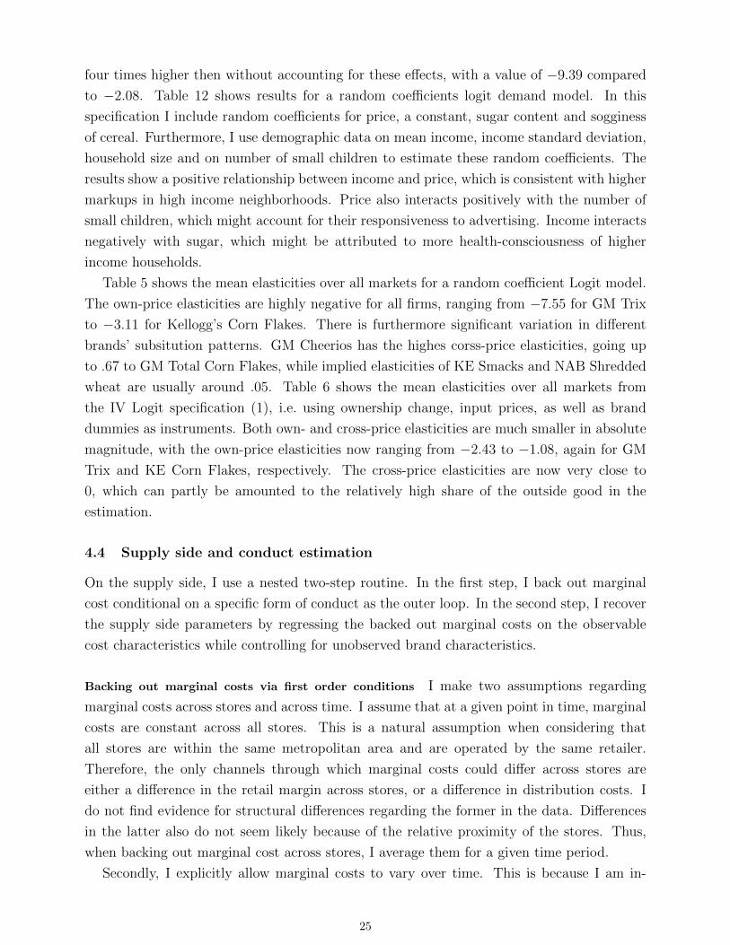
Implication of choice set In my dataset, I observe exit and entry of some brands. Table 7
shows the brand names as well as time of entry and exit. There are 11 entries and 5 exits
23

overall. Around week 130, which is about 10 months prior to the merger, 3 new private
label products and two national brands also become available in the Dominick’s stores. This
causes variation in the consumers’ choice spaces. Since I do not include these products in
my estimation, these entries should have effects on the substitutability from inside products
to the outside good. Furthermore, brands with a similar product characteristics should face
higher competition, which might cause a change in these prices.
Demand Elasticities Individual market shares depend on the mean utility as well as on the
random and demographic components.
sijt =exp(δjt + µijt)
1 +∑J
k=1 exp(δkt + µikt)(18)
Integrating over the whole distribution of individuals yields the aggregated market shares
from the model. The cross-price elasticity between goods j and k at time t, ηjkt, can be
written as
ηjkt =
−pjtsjt
∫αisijt(1− sijt)dPD(D)dPv(v) j = k
pktsjt
∫αisijtsiktdPD(D)dPv(v) j 6= k
(19)
There are several options to compute these elasticities depending on how much model
structure one wants to use. When using the random coefficients model, one needs to compute
the individual market shares using the model structure and equation (18). However, there
are two different options how to account for the aggregated market share sjt. Either one
integrates the individual market shares over all individuals, or uses the post merger market
share at time t together with the post-merger prices. In the second case, the only remaining
model component stems from the price coefficient α.
When using a regular Logit model instead of a Random Coefficient Logit model, all het-
erogeneity will be accounted for by the error term, such that the price elasticity of good j
with respect to good k at time t can be written as
ηjkt =
−pjtsjt
αsjt(1− sjt) j = k
pktsjtαsjtskt j 6= k
Estimates Table 2 shows demand side estimation results for several specifications of the
Logit model. Overall, using input prices, prices of other zones, brand characteristics or the
ownership change as instruments for the sales price in all but one specification yields a more
elastic demand curve than specification (3) without instruments. Accounting for brand-
specific fixed effects increases the the price-responsiveness even more dramatically. This can
be seen when comparing specifications (1) and (2). Both specifications use input prices and
the ownership change as instruments for the unobserved brand components. When accounting
for brand-specific fixed effects, however, the price coefficient is in absolute terms more than
24
four times higher then without accounting for these effects, with a value of −9.39 compared
to −2.08. Table 12 shows results for a random coefficients logit demand model. In this
specification I include random coefficients for price, a constant, sugar content and sogginess
of cereal. Furthermore, I use demographic data on mean income, income standard deviation,
household size and on number of small children to estimate these random coefficients. The
results show a positive relationship between income and price, which is consistent with higher
markups in high income neighborhoods. Price also interacts positively with the number of
small children, which might account for their responsiveness to advertising. Income interacts
negatively with sugar, which might be attributed to more health-consciousness of higher
income households.
Table 5 shows the mean elasticities over all markets for a random coefficient Logit model.
The own-price elasticities are highly negative for all firms, ranging from −7.55 for GM Trix
to −3.11 for Kellogg’s Corn Flakes. There is furthermore significant variation in different
brands’ subsitution patterns. GM Cheerios has the highes corss-price elasticities, going up
to .67 to GM Total Corn Flakes, while implied elasticities of KE Smacks and NAB Shredded
wheat are usually around .05. Table 6 shows the mean elasticities over all markets from
the IV Logit specification (1), i.e. using ownership change, input prices, as well as brand
dummies as instruments. Both own- and cross-price elasticities are much smaller in absolute
magnitude, with the own-price elasticities now ranging from −2.43 to −1.08, again for GM
Trix and KE Corn Flakes, respectively. The cross-price elasticities are now very close to
0, which can partly be amounted to the relatively high share of the outside good in the
estimation.
4.4 Supply side and conduct estimation
On the supply side, I use a nested two-step routine. In the first step, I back out marginal
cost conditional on a specific form of conduct as the outer loop. In the second step, I recover
the supply side parameters by regressing the backed out marginal costs on the observable
cost characteristics while controlling for unobserved brand characteristics.
Backing out marginal costs via first order conditions I make two assumptions regarding
marginal costs across stores and across time. I assume that at a given point in time, marginal
costs are constant across all stores. This is a natural assumption when considering that
all stores are within the same metropolitan area and are operated by the same retailer.
Therefore, the only channels through which marginal costs could differ across stores are
either a difference in the retail margin across stores, or a difference in distribution costs. I
do not find evidence for structural differences regarding the former in the data. Differences
in the latter also do not seem likely because of the relative proximity of the stores. Thus,
when backing out marginal cost across stores, I average them for a given time period.
Secondly, I explicitly allow marginal costs to vary over time. This is because I am in-
25

terested in finding the determinants for marginal costs pre-merger and then predicting post
merger prices using variation in input prices over time. Therefore, I recover marginal costs
over several pre-merger periods and use the estimates to predict post-merger also for different
post-merger periods. This is a further difference to conventional merger simulations. There,
one often only predicts the equilibrium for one post-merger period which also assumes only
one predicted vector of post-merger marginal costs.
Post-merger price equilibrium There are several ways to predict the price changes caused
by a merger. The main difference lies in how to account for post merger market shares.
I treat the observed post-merger prices in the data as equilibrium prices. Methodically
this is a fundamental difference to the existing literature regarding merger simulation. In
this literature, one usually simulates for a new price equilibrium using a specific form of
competition and the parameters recovered from the demand simulation. As a convergence
criterion one looks for a price vector that constitutes a mutual best response of prices given
the predicted market shares using demand estimates.13 There are several advantages from
using the actual post-merger prices instead of simulating a post-merger price equilibrium.
Firstly, when simulating for a new price equilibrium, one needs to make an assumption
regarding competition in the market. Already without estimating industry conduct, this is
computationally demanding. Furthermore, it does not make use of all the available post-
merger data, i.e. market shares and prices. Secondly, by using post-merger price simulation,
one also risks averaging out specific competitive patterns and introduces a simulation error.
Inner loop - cost parameter estimation In the second step of my supply side estimation
procedure, I use the marginal costs that were backed out conditional on a specific form of
industry conduct and estimate the marginal cost equation 8 via minimizing the following
GMM objective function:
γS = arg minγS
ω(Θ, γS, γD)′ZωA−1ω Z ′ωω(Θ, γS, γD). (20)
A−1ω is a consistent estimate of the covariance E[Z ′ωω(Θ, γS, γD)ω(Θ, γS, γD)′Zω]. The brand
specific marginal cost fixed effect ωj may be correlated with unobservable product charac-
teristics. Therefore it is essential to look for instruments that are correlated with marginal
costs, but not with the error term. To account for the effects of unobserved cost drivers on
prices, I use first order basis functions of the own brand characteristics, own firm characteris-
tics, and competitors’ characteristics. This relies on an exchangeability argument of product
characteristics when facing a unique Nash equilibrium, see for example Berry et al. (1995).
Outer loop - conduct estimation Having obtained the demand side coefficients γD and the
cost parameters γS for any form of industry conduct , I estimate the conduct parameters Θ
13An advantage of this approach is that it checks for consistency of prices and market shares in the post merger equilibrium.However, this approach neglects the available post-merger market shares and is computationally very intense.
26

by minimizing the GMM objective function which moments consists of the empirical own-
and cross-firm residuals ϕown and ϕcross interacted with the specific conduct parameters,
as described in section 3. Denote the combined vector of these two kinds of moments by
G(Θ, γS), where γS denotes the cost estimates from the second step that are conditional on
a specific form of conduct. Then the second stage GMM objective can be written as
Θ = arg minΘG(Θ, γS)′WG(Θ, γS), (21)
where W (Θ, γS) is a positive definite, asymptotically efficient weighting matrix given first-
stage estimates Θ and γS.
Conduct estimation results Table 3 shows the conduct estimation results under the assump-
tion of bilateral brand symmetry, with an input price IV logit demand side estimates being
used. Using this approach, all parameters are significant on a 99% level. The parameter esti-
mates range from .46 to .60, indicating a relatively cooperative form of industry conduct. The
implied median price-cost margins are very close to those implied by a full collusion model.
It is interesting to compare the implied price cost-margins to those from a multi-product
Nash pricing supply side model. Under multi-product Nash pricing, all of the markup can
be attributed to product differentiation, and not to cooperative effects. The implied median
price-cost margins from the estimation are 31.7% higher than the median multi-brand Nash
price cost margins. This indicates a powerful cooperative effect across different firms. The
results change when using a Logit specification without instruments, also see table 4 for the
results. Because of a lower estimated price-sensitivity, the specification’s implied price-cost
margins are higher. The median price-cost margin implied by the estimated conduct pa-
rameters is now closer to margins implied by multi-brand Nash pricing, with only an 8%
higher median margin. This is not surprising, as the lower price sensitivity implies a lower
substitutability and already higher industry markups in the absence of any cooperation.
5 Extensions
In this section I present extensions to my basic framework that address several,merger related
issues, some of which have not been touched before in the literature.
5.1 Supply side selection methods
Instead of testing for industry conduct directly, it is common in this literature to select among
a discrete set of different supply side models. A big advantage of this “menu” approach is
that it severely reduces the number of parameters that needs to be estimated. Furthermore, it
allows the researcher to restrict attention to models that have a clear economic interpretation,
such as multi-brand competition or partial collusion between firms.
27

(1) (2) (3) (4) (5) (6) (7)
price -9.39*** -2.08*** -5.09*** -22.6*** -6.56*** -8.79*** -5.22***(0.77) (0.25) (0.18) (1.57) (0.35) (0.24) (0.18)
quarter dummy 0.0034*** 0.00073 0.0016 0.0075*** 0.0020 0.0032*** 0.0016(0.00098) (0.0017) (0.0017) (0.0012) (0.0017) (0.00095) (0.0017)
sales 0.053*** 0.18*** 0.17*** -0.011 0.17*** 0.055*** 0.17***(0.0087) (0.013) (0.013) (0.012) (0.013) (0.0079) (0.013)
calories 0.0068*** 0.0064*** 0.0062*** 0.000072 0.0061*** 0.0071*** 0.0062***(0.00044) (0.00027) (0.00027) (0.00083) (0.00027) (0.00025) (0.00027)
mushy 1.51*** 1.06*** 0.95*** 1.01*** 0.89*** 1.48*** 0.94***(0.049) (0.020) (0.018) (0.11) (0.022) (0.027) (0.018)
sugars -0.0089*** -0.0016*** -0.00087* 0.00033 -0.00054 -0.0093*** -0.00084(0.00074) (0.00044) (0.00043) (0.0013) (0.00044) (0.00053) (0.00043)
income -0.080*** -0.071** -0.074*** -0.093*** -0.075*** -0.079*** -0.074***(0.013) (0.023) (0.022) (0.016) (0.022) (0.013) (0.022)
young child 0.34 1.19*** 0.85** -1.19*** 0.68* 0.41** 0.83**(0.17) (0.27) (0.26) (0.26) (0.27) (0.15) (0.26)
N 11760 11760 11760 11760 11760 11760 11760R2 0.78 0.31 0.33 0.68 0.33 0.78 0.33
Input price IV Yes Yes No No No No NoCost characteristics IV No No No Yes Yes No No
Zone IV No No No No No Yes YesOwnership IV Yes Yes No Yes Yes No No
Brand dummies Yes No No Yes No Yes No
Table 2: Demand estimation results for different Logit specifications
Firm A Firm B Firm C Firm D Firm E Firm F
Firm A 1 .52*** .60*** .50*** .46*** .47***Firm B 1 .51*** .46*** .57*** .46***Firm C 1 .56*** .52*** .47***Firm D 1 .57*** .52***Firm E 1 .54***Firm F 1
Type of competition Median PCM Std. Dev PCMEstimated Conduct .44 .07Multi-brand Nash .30 .05Full collusion .45 .08
Table 3: Conduct estimates under bilateral firm symmetry, IV Logit demand
Firm A Firm B Firm C Firm D Firm E Firm F
Firm A 1 .46*** .50*** .51*** .54*** .48***Firm B 1 .46*** .53*** .58*** .51***Firm C 1 .49*** .52*** .52***Firm D 1 .48*** .48***Firm E 1 .54***Firm F 1
Type of competition Median PCM Std. Dev PCMEstimated Conduct .72 .10Multi-brand Nash .67 .09Full collusion .89 .8
Table 4: Conduct estimates under bilateral firm symmetry, Logit demand
28

NAB NAB PO PO PO GM GM GM GM GM GM GM GM KEShW SSW GNu RBr RNB Hon ACh Whe Che HNC LCh TCF Tri FLo
NAB Shred Wheat -5.56 0.15 0.13 0.06 0.09 0.11 0.11 0.07 0.54 0.30 0.19 0.23 0.15 0.19NAB Sp Shr Whea 0.07 -5.49 0.14 0.06 0.09 0.11 0.12 0.08 0.56 0.30 0.19 0.24 0.16 0.20PO Grape Nuts 0.05 0.11 -4.03 0.06 0.06 0.08 0.09 0.07 0.36 0.24 0.12 0.13 0.09 0.14PO Raisin Bran 0.03 0.06 0.07 -4.84 0.06 0.06 0.08 0.16 0.21 0.20 0.13 0.10 0.10 0.13PO Honeycomb 0.06 0.14 0.11 0.08 -6.82 0.12 0.15 0.10 0.55 0.37 0.25 0.27 0.22 0.26GM RaisNut Bran 0.06 0.13 0.12 0.07 0.10 -5.67 0.13 0.09 0.48 0.32 0.21 0.21 0.17 0.22GM AppCin Cheer 0.05 0.12 0.11 0.08 0.11 0.11 -6.01 0.10 0.47 0.35 0.22 0.22 0.19 0.24GM Wheaties 0.03 0.07 0.08 0.14 0.06 0.07 0.09 -4.89 0.27 0.22 0.13 0.12 0.11 0.14GM Cheerios 0.07 0.16 0.13 0.06 0.10 0.11 0.13 0.08 -5.59 0.34 0.21 0.26 0.18 0.22GM HonNut Cheer 0.05 0.12 0.12 0.08 0.10 0.11 0.14 0.10 0.48 -5.59 0.21 0.21 0.18 0.23GM Luck Charms 0.06 0.13 0.11 0.08 0.12 0.12 0.16 0.10 0.53 0.37 -6.59 0.26 0.22 0.26GM TCorn Flakes 0.07 0.17 0.11 0.06 0.13 0.13 0.15 0.09 0.67 0.38 0.26 -7.41 0.24 0.26GM Trix 0.06 0.14 0.10 0.08 0.13 0.13 0.17 0.11 0.58 0.39 0.28 0.30 -7.55 0.28KE Froot Loops 0.05 0.12 0.11 0.08 0.11 0.12 0.15 0.10 0.51 0.36 0.24 0.24 0.21 -6.22KE Special K 0.05 0.10 0.08 0.13 0.10 0.09 0.12 0.17 0.42 0.30 0.21 0.22 0.19 0.21KE Frost Flakes 0.02 0.05 0.06 0.15 0.05 0.06 0.08 0.16 0.19 0.19 0.12 0.08 0.09 0.12KE Corn Pops 0.05 0.12 0.11 0.08 0.11 0.11 0.15 0.10 0.49 0.36 0.23 0.23 0.21 0.25KE Raisin Bran 0.02 0.04 0.06 0.15 0.04 0.05 0.07 0.15 0.16 0.17 0.10 0.07 0.08 0.11KE Corn Flakes 0.02 0.04 0.07 0.12 0.03 0.04 0.05 0.13 0.14 0.13 0.07 0.05 0.05 0.08KE Smacks 0.05 0.10 0.11 0.10 0.10 0.11 0.14 0.11 0.39 0.33 0.22 0.18 0.17 0.22KE Crispix 0.07 0.16 0.12 0.06 0.12 0.12 0.14 0.09 0.61 0.34 0.23 0.29 0.20 0.24KE JRight Fruit 0.06 0.13 0.13 0.07 0.10 0.11 0.13 0.09 0.48 0.32 0.20 0.21 0.16 0.21KE Nutri Grain 0.06 0.12 0.12 0.08 0.10 0.11 0.13 0.09 0.45 0.33 0.21 0.20 0.17 0.21RA Corn Chex 0.07 0.16 0.12 0.06 0.12 0.12 0.14 0.09 0.62 0.36 0.24 0.30 0.21 0.24RA Wheat Chex 0.06 0.14 0.14 0.06 0.08 0.10 0.11 0.08 0.47 0.29 0.17 0.19 0.13 0.18RA Rice Chex 0.08 0.16 0.12 0.06 0.12 0.12 0.14 0.09 0.63 0.35 0.24 0.30 0.21 0.24QO 100 Natural 0.04 0.09 0.13 0.06 0.06 0.08 0.09 0.07 0.32 0.23 0.12 0.11 0.09 0.14QO Capn Crunch 0.04 0.10 0.12 0.08 0.08 0.10 0.12 0.09 0.36 0.30 0.18 0.15 0.14 0.19
KE KE KE KE KE KE KE KE KE RA RA RA QO QOSpK FFl CPo RBr CFl Sma Cri JRi NGr CCh WCh RCh QO1 CCr
NAB Shred Wheat 0.22 0.17 0.15 0.11 0.12 0.04 0.16 0.06 0.05 0.08 0.05 0.11 0.10 0.13NAB Sp Shr Whea 0.21 0.17 0.15 0.11 0.11 0.04 0.16 0.06 0.05 0.08 0.05 0.11 0.10 0.13PO Grape Nuts 0.13 0.18 0.11 0.13 0.14 0.03 0.10 0.04 0.04 0.05 0.04 0.06 0.12 0.13PO Raisin Bran 0.30 0.53 0.12 0.35 0.31 0.04 0.07 0.03 0.03 0.03 0.02 0.04 0.07 0.11PO Honeycomb 0.31 0.27 0.21 0.16 0.12 0.06 0.17 0.06 0.06 0.09 0.04 0.11 0.09 0.16GM RaisNut Bran 0.24 0.24 0.17 0.15 0.13 0.05 0.15 0.06 0.05 0.07 0.04 0.09 0.11 0.15GM AppCin Cheer 0.26 0.28 0.19 0.17 0.14 0.05 0.14 0.06 0.06 0.07 0.04 0.09 0.10 0.16GM Wheaties 0.31 0.49 0.11 0.33 0.29 0.04 0.08 0.03 0.03 0.04 0.03 0.05 0.07 0.11GM Cheerios 0.25 0.19 0.17 0.11 0.11 0.04 0.18 0.06 0.05 0.09 0.05 0.12 0.10 0.13GM HonNut Cheer 0.25 0.26 0.18 0.16 0.14 0.05 0.14 0.06 0.05 0.07 0.04 0.09 0.10 0.16GM Luck Charms 0.31 0.29 0.21 0.16 0.13 0.06 0.17 0.06 0.06 0.08 0.04 0.11 0.09 0.16GM TCorn Flakes 0.32 0.21 0.20 0.12 0.10 0.05 0.21 0.07 0.06 0.10 0.05 0.14 0.09 0.14GM Trix 0.34 0.28 0.22 0.16 0.11 0.06 0.18 0.06 0.06 0.09 0.04 0.12 0.08 0.16KE Froot Loops 0.28 0.28 0.20 0.17 0.13 0.05 0.15 0.06 0.06 0.08 0.04 0.10 0.10 0.16KE Special K -6.51 0.45 0.17 0.27 0.22 0.05 0.14 0.05 0.05 0.07 0.03 0.09 0.07 0.13KE Frost Flakes 0.28 -4.36 0.11 0.38 0.31 0.04 0.06 0.03 0.03 0.03 0.02 0.04 0.07 0.11KE Corn Pops 0.28 0.29 -6.27 0.17 0.14 0.05 0.15 0.06 0.06 0.07 0.04 0.10 0.10 0.16KE Raisin Bran 0.24 0.53 0.09 -4.04 0.32 0.03 0.05 0.03 0.03 0.02 0.02 0.03 0.07 0.10KE Corn Flakes 0.18 0.42 0.07 0.31 -3.11 0.02 0.04 0.02 0.02 0.02 0.02 0.03 0.07 0.08KE Smacks 0.26 0.33 0.18 0.20 0.16 -5.95 0.13 0.05 0.06 0.06 0.04 0.08 0.10 0.17KE Crispix 0.28 0.20 0.18 0.12 0.11 0.05 -6.62 0.06 0.06 0.10 0.05 0.13 0.09 0.14KE JRight Fruit 0.23 0.23 0.17 0.14 0.13 0.05 0.15 -5.60 0.05 0.07 0.05 0.09 0.10 0.15KE Nutri Grain 0.24 0.26 0.18 0.16 0.14 0.05 0.14 0.06 -5.76 0.07 0.04 0.09 0.10 0.15RA Corn Chex 0.28 0.20 0.19 0.12 0.11 0.05 0.19 0.06 0.06 -6.83 0.05 0.13 0.09 0.14RA Wheat Chex 0.19 0.19 0.14 0.12 0.13 0.04 0.14 0.05 0.05 0.07 -5.09 0.09 0.11 0.13RA Rice Chex 0.28 0.20 0.19 0.11 0.10 0.05 0.19 0.06 0.06 0.10 0.05 -6.83 0.09 0.14QO 100 Natural 0.13 0.21 0.11 0.14 0.16 0.03 0.09 0.04 0.04 0.04 0.04 0.05 -3.92 0.13QO Capn Crunch 0.20 0.29 0.15 0.18 0.16 0.05 0.11 0.05 0.05 0.05 0.04 0.07 0.11 -5.05
Table 5: Mean Elasticities RC Logit
29

NAB NAB PO PO PO GM GM GM GM GM GM GM GM KEShW SSW GNu RBr RNB Hon ACh Whe Che HNC LCh TCF Tri FLo
NAB Shred Wheat -1.77 0.01 0.01 0.01 0.00 0.01 0.01 0.01 0.02 0.02 0.01 0.01 0.01 0.01NAB Sp Shr Whea 0.00 -1.78 0.01 0.01 0.00 0.01 0.01 0.01 0.02 0.02 0.01 0.01 0.01 0.01PO Grape Nuts 0.00 0.01 -1.32 0.01 0.00 0.00 0.00 0.01 0.02 0.01 0.01 0.01 0.00 0.01PO Raisin Bran 0.00 0.01 0.01 -1.57 0.00 0.00 0.01 0.01 0.02 0.01 0.01 0.01 0.00 0.01PO Honeycomb 0.00 0.01 0.02 0.01 -2.17 0.01 0.01 0.01 0.03 0.02 0.01 0.01 0.01 0.01GM RaisNut Bran 0.00 0.01 0.01 0.01 0.00 -1.82 0.01 0.01 0.02 0.02 0.01 0.01 0.01 0.01GM AppCin Cheer 0.00 0.01 0.01 0.01 0.00 0.01 -1.93 0.01 0.02 0.02 0.01 0.01 0.01 0.01GM Wheaties 0.00 0.01 0.01 0.01 0.00 0.01 0.01 -1.60 0.02 0.01 0.01 0.01 0.00 0.01GM Cheerios 0.00 0.01 0.01 0.01 0.00 0.01 0.01 0.01 -1.92 0.02 0.01 0.01 0.01 0.01GM HonNut Cheer 0.00 0.01 0.01 0.01 0.00 0.01 0.01 0.01 0.02 -1.85 0.01 0.01 0.01 0.01GM Luck Charms 0.00 0.01 0.02 0.01 0.00 0.01 0.01 0.01 0.03 0.02 -2.14 0.01 0.01 0.01GM TCorn Flakes 0.00 0.01 0.02 0.01 0.00 0.01 0.01 0.01 0.03 0.02 0.01 -2.40 0.01 0.01GM Trix 0.00 0.01 0.02 0.01 0.00 0.01 0.01 0.01 0.03 0.02 0.01 0.01 -2.43 0.01KE Froot Loops 0.00 0.01 0.01 0.01 0.00 0.01 0.01 0.01 0.03 0.02 0.01 0.01 0.01 -2.03KE Special K 0.00 0.01 0.02 0.01 0.00 0.01 0.01 0.01 0.03 0.02 0.01 0.01 0.01 0.01KE Frost Flakes 0.00 0.01 0.01 0.01 0.00 0.01 0.01 0.01 0.02 0.01 0.01 0.01 0.00 0.01KE Corn Pops 0.00 0.01 0.01 0.01 0.00 0.01 0.01 0.01 0.03 0.02 0.01 0.01 0.01 0.01KE Raisin Bran 0.00 0.01 0.01 0.01 0.00 0.00 0.00 0.01 0.02 0.01 0.01 0.01 0.00 0.01KE Corn Flakes 0.00 0.00 0.01 0.00 0.00 0.00 0.00 0.01 0.01 0.01 0.00 0.00 0.00 0.01KE Smacks 0.00 0.01 0.01 0.01 0.00 0.01 0.01 0.01 0.02 0.02 0.01 0.01 0.01 0.01KE Crispix 0.00 0.01 0.02 0.01 0.00 0.01 0.01 0.01 0.03 0.02 0.01 0.01 0.01 0.01KE JRight Fruit 0.00 0.01 0.01 0.01 0.00 0.01 0.01 0.01 0.02 0.02 0.01 0.01 0.01 0.01KE Nutri Grain 0.00 0.01 0.01 0.01 0.00 0.01 0.01 0.01 0.02 0.02 0.01 0.01 0.01 0.01RA Corn Chex 0.00 0.01 0.02 0.01 0.00 0.01 0.01 0.01 0.03 0.02 0.01 0.01 0.01 0.01RA Wheat Chex 0.00 0.01 0.01 0.01 0.00 0.01 0.01 0.01 0.02 0.02 0.01 0.01 0.00 0.01RA Rice Chex 0.00 0.01 0.02 0.01 0.00 0.01 0.01 0.01 0.03 0.02 0.01 0.01 0.01 0.01QO 100 Natural 0.00 0.01 0.01 0.01 0.00 0.00 0.00 0.01 0.02 0.01 0.01 0.00 0.00 0.01QO Capn Crunch 0.00 0.01 0.01 0.01 0.00 0.01 0.01 0.01 0.02 0.02 0.01 0.01 0.00 0.01
KE KE KE KE KE KE KE KE KE RA RA RA QO QOSpK FFl CPo RBr CFl Sma Cri JRi NGr CCh WCh RCh QO1 CCr
NAB Shred Wheat 0.01 0.02 0.01 0.02 0.03 0.00 0.01 0.00 0.00 0.00 0.00 0.00 0.01 0.01NAB Sp Shr Whea 0.01 0.02 0.01 0.02 0.03 0.00 0.01 0.00 0.00 0.00 0.00 0.00 0.01 0.01PO Grape Nuts 0.01 0.02 0.01 0.02 0.02 0.00 0.00 0.00 0.00 0.00 0.00 0.00 0.01 0.01PO Raisin Bran 0.01 0.02 0.01 0.02 0.02 0.00 0.01 0.00 0.00 0.00 0.00 0.00 0.01 0.01PO Honeycomb 0.01 0.03 0.01 0.03 0.03 0.00 0.01 0.00 0.00 0.00 0.00 0.00 0.01 0.01GM RaisNut Bran 0.01 0.03 0.01 0.02 0.03 0.00 0.01 0.00 0.00 0.00 0.00 0.00 0.01 0.01GM AppCin Cheer 0.01 0.03 0.01 0.02 0.03 0.00 0.01 0.00 0.00 0.00 0.00 0.00 0.01 0.01GM Wheaties 0.01 0.02 0.01 0.02 0.02 0.00 0.01 0.00 0.00 0.00 0.00 0.00 0.01 0.01GM Cheerios 0.01 0.03 0.01 0.02 0.03 0.00 0.01 0.00 0.00 0.00 0.00 0.00 0.01 0.01GM HonNut Cheer 0.01 0.03 0.01 0.02 0.03 0.00 0.01 0.00 0.00 0.00 0.00 0.00 0.01 0.01GM Luck Charms 0.01 0.03 0.01 0.03 0.03 0.00 0.01 0.00 0.00 0.00 0.00 0.00 0.01 0.01GM TCorn Flakes 0.02 0.03 0.01 0.03 0.04 0.00 0.01 0.00 0.00 0.00 0.00 0.00 0.02 0.01GM Trix 0.02 0.03 0.01 0.03 0.04 0.00 0.01 0.00 0.00 0.00 0.00 0.00 0.02 0.01KE Froot Loops 0.01 0.03 0.01 0.02 0.03 0.00 0.01 0.00 0.00 0.00 0.00 0.00 0.01 0.01KE Special K -2.15 0.03 0.01 0.03 0.03 0.00 0.01 0.00 0.00 0.00 0.00 0.00 0.01 0.01KE Frost Flakes 0.01 -1.54 0.01 0.02 0.02 0.00 0.01 0.00 0.00 0.00 0.00 0.00 0.01 0.01KE Corn Pops 0.01 0.03 -2.03 0.02 0.03 0.00 0.01 0.00 0.00 0.00 0.00 0.00 0.01 0.01KE Raisin Bran 0.01 0.02 0.01 -1.39 0.02 0.00 0.00 0.00 0.00 0.00 0.00 0.00 0.01 0.01KE Corn Flakes 0.01 0.02 0.00 0.01 -1.08 0.00 0.00 0.00 0.00 0.00 0.00 0.00 0.01 0.01KE Smacks 0.01 0.03 0.01 0.02 0.03 -1.89 0.01 0.00 0.00 0.00 0.00 0.00 0.01 0.01KE Crispix 0.01 0.03 0.01 0.03 0.03 0.00 -2.12 0.00 0.00 0.00 0.00 0.00 0.01 0.01KE JRight Fruit 0.01 0.02 0.01 0.02 0.03 0.00 0.01 -1.78 0.00 0.00 0.00 0.00 0.01 0.01KE Nutri Grain 0.01 0.03 0.01 0.02 0.03 0.00 0.01 0.00 -1.83 0.00 0.00 0.00 0.01 0.01RA Corn Chex 0.01 0.03 0.01 0.03 0.03 0.00 0.01 0.00 0.00 -2.17 0.00 0.00 0.01 0.01RA Wheat Chex 0.01 0.02 0.01 0.02 0.02 0.00 0.01 0.00 0.00 0.00 -1.63 0.00 0.01 0.01RA Rice Chex 0.02 0.03 0.01 0.03 0.03 0.00 0.01 0.00 0.00 0.00 0.00 -2.18 0.01 0.01QO 100 Natural 0.01 0.02 0.01 0.02 0.02 0.00 0.00 0.00 0.00 0.00 0.00 0.00 -1.29 0.01QO Capn Crunch 0.01 0.02 0.01 0.02 0.03 0.00 0.01 0.00 0.00 0.00 0.00 0.00 0.01 -1.65
Table 6: Mean Elasticities IV Logit
30

There are two popular methods to select among a set of non-nested supply side models.
The first method compares the marginal cost estimates of the different supply side specifica-
tions with cost estimates from other sources, such as accounting data, see for example Nevo
(2001). At first sight this seems to be an intuitive way to select the most appropriate speci-
fication from the data. This approach, however, has several weaknesses. Firstly, outside cost
estimates are not always available, or do not give a reliable economic interpretation. Fur-
thermore, such data is often only available on a very aggregate level, which makes a detailed
industry introspective nearly impossible.14 Thirdly, if different specifications yield similar
cost estimates, it is not clear how one can use these results for a reliable model selection.
The second method uses forms of non-nested selection test to look pre-merger for the
supply specification that is closest to the true data generating process, see for example Vuong
(1989) or Rivers and Vuong (2002). One problem of this method is that one cannot easily
see where different non-nested specifications do better or worse, respectively, in replicating
the true data-generating process. Furthermore, in practice such tests have relatively low
predictive power.
My identification assumption and data structure gives rise to an additional selection
method. I can predict the post-merger prices for each form of proposed equilibrium given
pre-merger data, and then compare them with the actual post-merger prices. There are sev-
eral advantages of this method compared to the other approaches. This method provides a
tractable in-sample test. Thus, I do not need out of sample data to select among different
non-nested models, and can also check where the different specifications have strengths and
weaknesses. Testing can then be done using a J-Test or using a variant of the Rivers and
Vuong (2002) approach.
Formal Rivers and Vuong approach Consider a non-nested conduct specification h, with
conduct matrix Θh. One can recover the marginal cost using p − Ω−1(Θh)s. Furthermore,
using my marginal cost specification, one obtains mchjt = w′jtγS + ωhj + εhjt.
With E[εhjt|ωhj , wjt] = 0, γSh , ωj, and εhjt can be consistently estimated.
Infer a cost equation with best statistical fit given the observed shifters that depend on
the specific brand characteristics, but not on the “conjectured” model. If one tests between
two different models,
pjt = Ω−1(Θh)s+ w′jtγSh + ωhj + εhjt
p′
jt = Ω−1(Θh′)s+ w′jtγSh′ + ωh
′
j + εh′
jt
minγSh ,ω
hj
Qhn(γSh′ , ω
hj ) = min
γSh ,ωhj
1
n
∑j,t
εhjt =1
n
∑j,t
[pjt − Ω−1(Θh)s− ωhj − w′jtγSh ]2
This does not require any of the specifications h, h′ to be correctly specified. Denote by
Qh
n(γSh , ωhj ) the expected lack-of-fit criteria (opposite of goodness of fit).
14Nevo (2001) states that his data is not sufficiently detailed to test for collusion among a subset of firms.
31

H0 : h and h′are asymptotically equivalent ifH0 : limn→∞Q
h
n(γSh , ωhj )−Q
h′
n (γSh′ , ωh′j ) = 0
H1 : h asymptotically better fit than h′ if limn→∞Qh
n(γSh , ωhj )−Q
h′
n (γSh′ , ωh′j ) < 0
H2 : h′ asymptotically better fit than h if limn→∞Qh
n(γSh , ωhj )−Q
h′
n (γSh′ , ωh′j ) > 0
Test statistic Tn captures statistical variation that characterizes sample value of lack-of-fit
criterion and is then defined as a suitable difference of the sample lack-of-fit criteria:
Tn =
√n
σhh′n
Qh
n(γSh , ωhj )−Q
h′
n (γSh′ , ωh′
j ), (22)
where σhh′
n denotes the estimated value of the variance fo the difference in the lack-of-fit
criterion.
Rivers and Vuong show that if two models are strictly non-nested, the asymptotic distri-
bution of Tn is standard normal. Thus, one has to compare sample values of Tn with the
critical values of a standard normal distribution.
5.2 Welfare implications
A natural question to ask post-merger is whether the Post-Nabisco merger had an impact
on consumer welfare.15 To answer this question I have to make strong assumptions for a
counterfactual analysis in case the merger had not been approved. The first assumption
concerns the retail margin. As Figure 9 shows, my measure for the average retail margin
significantly drops for approximately 4 quarters after the merger before it goes up again. If
this drop in retail margin is caused by the merger, I have to correct for such a drop in a
counterfactual analysis. Furthermore, when considering long run effects, there is the question
whether the price war started by Post-Nabisco in 1997 would have happened without the
merger having taken place. To fully understand the underlying drivers of this price war, I
would have to account for several explanations, such as firm synergies, and the impact of a
dramatic price decrease on persistent change in market share. TBC...
5.3 Post-merger profit internalization of merging firms
An implicit assumptions made in conventional merger simulations and also so far in this
paper is that firms will fully internalize the profits for all of their brands. Thus, a merger will
involve a change in the pricing strategies of the merged entity. Whereas this is rational from
a macroscopic view on a merged entity, economic theory also provides several explanations
for why this might not be the case.
From the principal-agent theory, it can be profitable for the principal to keep several
different profit centers inside of a firm. Because managers of a certain devision often have
performance based contracts and may also compete with their peers for higher management
positions, this may cause merging firms to not fully internalize their profits. Furthermore,
15Naturally, one can also ask the impact on overall welfare, which includes industry profits. Since the consumer welfare is themost common benchmark used, I will abstract from a full welfare analysis.
32

a coordination of prices within a merged firm may take some time due to difficulties in
post-merger integration.
Conditional on a specific form of industry-conduct between firms, my identification method
allows me to test for the intra-firm conduct post-merger. Consider an example with 3 firms,
in which firm 1 initially owns 2 brands. Furthermore, I assume that firms compete in multi-
product Nash pricing before and after the merger. Under these assumptions, the pre-merger
industry conduct matrix can be written as
Θpre =
1 1 0 0
1 1 0 0
0 0 1 0
0 0 0 1
Assume that firms 2 and 3 merge, and that the degree of post-merger profit internalization
θ is not observable to the researcher. Then the post merger conduct matrix turns to
Θpost = b(Θ) =
1 1 0 0
1 1 0 0
0 0 1 θ
0 0 θ 1
Under the assumption that synergies regarding merging firms’ marginal costs are either known
or not present, I can estimate intra-firm conduct using a variant of the GMM estimator
introduced above.
ϕiif (Θ, γS, γD) ≡ 1
TN
ST∑t=1
1
Jf
∑i∈Ff
(pposti,t (Θ, γS, γD)− pposti,t ).
As an identification condition for intra-firm conduct, I use orthogonality conditions between
the residual of observed and predicted prices and the intra-firm conduct parameters. These
conditions are similar to those when estimating industry conduct.
E[ϕiif (Θ, γS, γD)|df ] = 0 ∀i ∈ Ff (23)
5.4 Direct estimation of synergies
From an antitrust viewpoint, the magnitude of synergies plays a key role for the welfare and
consumer welfare effects of horizontal mergers, see for example Farrell and Shapiro (1990)
and Nocke and Whinston (2010).16 To my knowledge there is no approach that uses a
differentiated goods framework to estimate the magnitude of merger related marginal cost
16One example for an industry with significant synergies is the beer industry. After the 2005 Coors-Molson merger, thecompany stated that it made 66 million $ worth merger related synergies in its first year as joined entity.
33

synergies directly. I propose the following estimation method. Assume that industry conduct
is known in an industry pre-merger and post-merger. When accounting for the change in
price elasticities and the change in conduct after the merger, I can back out marginal costs
both pre-merger and post merger via the vector of first-order conditions. When conduct and
demand is known, the only systematic change can occur with respect to marginal costs. I will
use information on the timing of the merger to assess the impact of the merger on marginal
costs of the merging firms, which in economic terms reflects cost synergies.
Denote Θpre and Θpost the known pre- and post-merger industry conduct, respectively.
Then, using equation 8, I can back out the pre-merger and post-merger marginal cost from
the model:
mcpre = ppre − Ω−1(Θpre)spre
mcpost = ppost − Ω−1(Θpost)spost
Define mcall as the marginal cost vector both pre- and post-merger: mcall ≡ [mcpre;mcpost].
Recall the unobservable cost component ω. It might be that the unobservable cost component
changes for merging firms due to the merger. I assume that the merger will cause no change
in the unobserved cost components for the different brands.17
I will propose four different specification to estimate for synergies between merging firms.
1. Synergies in observable characteristics If one assumes that synergies will affect all ob-
servable brand characteristics in the same way, but will not affect unobserved brand charac-
teristics, then one can estimate the following equation:
mcj = (1 + κ1merge,j)(γSwj) + ωj, (24)
where κ represents the change in the observable brand characteristics on input prices, and
1merge is an indicator function equal to one if the brand belongs to one of the merging firms
in the post-merger periods.
2. Synergies in output A second possibility to account for synergies is to test for returns
to scale in total firm output. This can account for increasing returns to scale in distribution
cost or advertising. In this case, the marginal cost for brand j of firm f can be written as
mcj = τ∑i∈Ff
log(qi) + γSwj + ωj, (25)
17There is one way I could also account for a change in the unobserved cost component. As I use own-firm and competitors’product characteristics to form cost side instruments, the merger will cause variation in these instruments. If I assume that post-merger product characteristics will still be uncorrelated with the cost components, I can use the change in product characteristicsto identify the change in unobserved costs. Since this exogeneity of the product space is not realistic in the short run after amerger, I will not consider this assumption.
34

where qi denotes the total quantity sold of brand i. Since I only observe output in one
metropolitan area and brand, I have to assume that my data is representative for the average
output over all retailers in the industry.
3. Synergies in specific variables of merging firms I can also use a specification that only
allows specific observable factors to experience synergies due to a merger.
mcj = γSwj + ωj + 1merge,j1preψprei wi + 1merge,j1
postψposti (26)
6 Discussion
In this paper I have proposed a new approach to estimate industry conduct. The biggest
difference compared to other approaches lies in exploiting supply-side shifts using both pre-
and post-merger industry data and thereby inferring the underlying industry conduct. An
interesting feature of my data is the availability of a retail margin proxy. The sharp decline in
the retail margin during the time of the merger for most of the firms is a puzzling feature. In
general, the assumption that all retail margins are common knowledge is probably stronger
than the assumption regarding the common knowledge of marginal costs. While knowledge of
rivals’ marginal cost can be justified by the similar production processes, a producer’s retail
margin is also a result of bargaining between upstream and downstream firms. While my
data does not suggest a higher degree of bargaining power for a merged entity towards the
retailer, exploring the determinants of market power in more detail seems to be an important
task for future work.
Another important point of discussion concerns the direct estimation of firm synergies.
Using post-merger data and sufficiently many degrees of freedom, one can estimate firm
synergies for the merging firms. In this context, one important question is how to account
for economies of scale after the merger. It is unclear whether or how fast a merged entity
can adjust its production line to reduce costs. This is especially important in energy-intense
industries like the RTE cereal industry, and should also affect the firms’ pricing decisions.
One of the underlying identification assumptions is that overall industry conduct does not
change due to the merger. The fact that three years after the merger severe price cuts were
possible in the industry gives an indication for a relatively high markup over marginal cost
before.
The price cuts by Post-Nabisco in 1996 have several implications. Firstly, the results
suggest that all of the main players priced significantly over marginal costs before April
1996. One explanation consistent with Post’s price cuts would be stronger synergies of
production after the merger that made a defection from a relatively cooperative equilibrium
profitable. Secondly, the results seem to be fairly consistent with a change in equilibrium
only occurring after April 1996. Thirdly, this can be considered as another example for the
differences between short and long term implications of merger policies. With regard to the
35

last point, surprisingly little work has been done on the supply side dynamics in industries
due to mergers or other regulations. This also holds for testing the assumption of post-merger
profit internalization after a merger as well as the estimation of synergies, as discussed in the
extension. However, these are crucial factors in determining a merger’s effect on consumer
welfare. Since modern antitrust decisions sometimes heavily rely on econometric models, I
think that from an applied standpoint more work should be done in exploring these supply
side effects.
36

Figure 2: Price developments including promotions
A Additional information on data and estimation routines
B Rank conditions examples
In this section I present further examples that highlight the effects of the assumptions made
above. The main question will be under which circumstances marginal costs and industry
conduct will be jointly identified in a model.
3 firms, brands 1 and 2 belong to same firm Consider an industry that consists of 4 brands,
where brands 1 and 2 belong to the same firm. For simplicity, assume in this example
that marginal costs are constant for each firm. Furthermore, denote by pi,mci, si the price,
marginal costs and market share of firm i, respectively. θij describes the degree to which
brand i takes into account the profits of brand j when making its decision. In the example,
the maximization problem of brand 1 thus yields
maxp1
(p1 −mc1)s1(p) + p2 −mc2)s2(p) + θ13(p3 −mc3)s3(p) + θ14(p4 −mc4)s4(p)
The first-order condition for brand 1 with respect to its price then yields
(p1 −mc1)∂s1
∂p1
+ s1 + (p2 −mc2)∂s2
∂p1
+ θ13(p3 −mc3)∂s3
∂p1
+ θ14(p4 −mc4)∂s4
∂p1
= 0
37

Figure 3: Price development excluding promotions
Figure 4: Market shares for different firms
38
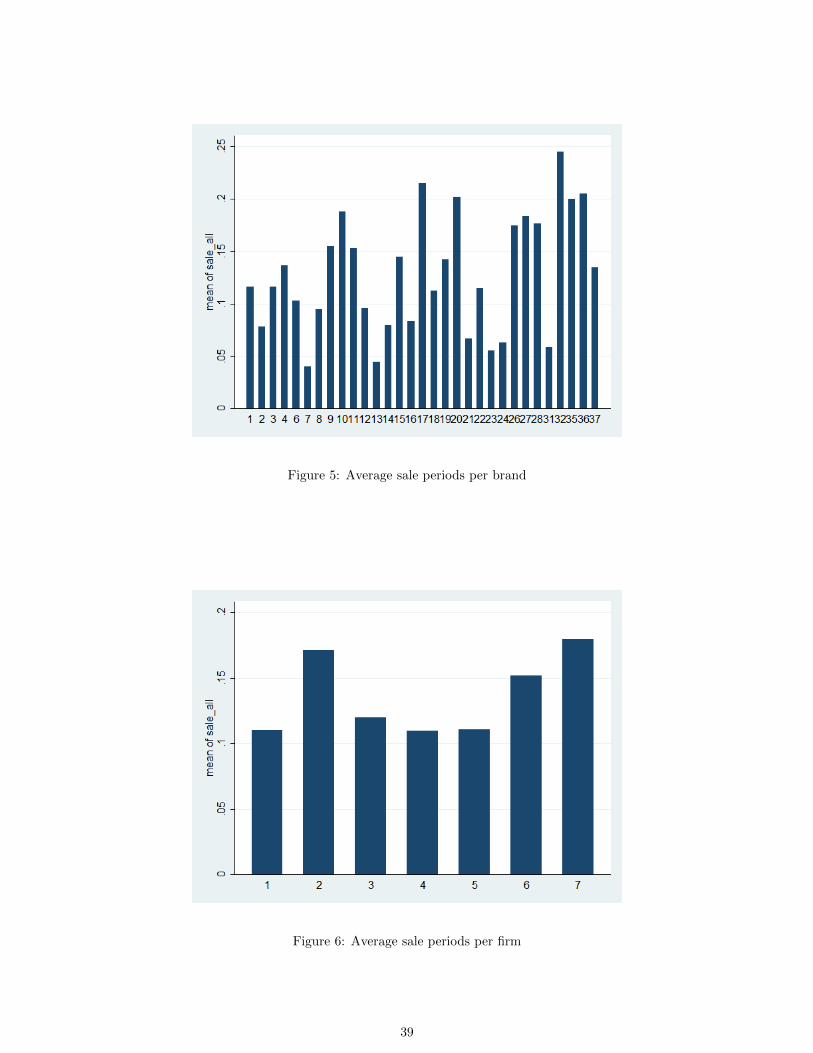
Figure 5: Average sale periods per brand
Figure 6: Average sale periods per firm
39
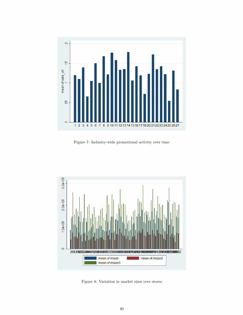
Figure 7: Industry-wide promotional activity over time
Figure 8: Variation in market sizes over stores
40

Assuming that each brand maximizes its own profits, the pre-merger conduct matrix yields
Θ =
1 θ12 θ13 θ14
θ21 1 θ23 θ24
θ31 θ32 1 θ34
θ41 θ42 θ43 1
When making the additional assumption that a firm maximizes the profits of all of its
brands, the pre-merger conduct matrix is
Θ =
1 1 θ13 θ14
1 1 θ23 θ24
θ31 θ32 1 θ34
θ41 θ42 θ43 1
There is a change in the ownership matrix pre- and post-merger if firms 2 and 3 merge. The
associated post-merger matrix yields
Θpost = b(Θ) =
1 1 θ13 θ14
1 1 θ23 θ24
θ31 θ32 1 1
θ41 θ42 1 1
From firm 1’s first order condition, conditional on the form of industry conduct, firms will
adapt their prices after an ownership change. In the above example, without symmetry, there
are 10 parameters to estimate, with only 4 equations, such that the rank conditions are never
met for identification. I introduce different assumption on firm supply to reduce the number
of parameters to be estimated.
Bilateral symmetry between firms Instead of bilateral brand symmetry, as stricter assump-
tion is that for all brands of two distinct firms, each brand will take the other firms’ brands
into account in the same fashion when making its pricing decision. Pre-merger conduct can
be written as
Θ =
1 1 θa θb
1 1 θa θb
θa θa 1 θc
θb θb θc 1
41

Post-merger conduct in this case is
Θpost = b(Θ) =
1 1 θa θb
1 1 θa θb
θa θa 1 1
θb θb 1 1
This leads to a number of 3 parameters to estimate, with 4 available equations, such that
the system is identified in absence of multi-collinearity.
Symmetry among all cross-firm brands When assuming that all brands take the brands of
all other firms into account in the same way, this results in the following pre-merger conduct:
Θ =
1 1 θa θa
1 1 θa θa
θa θa 1 θa
θa θa θa 1
.
Post-merger conduct is then
Θpost = b(Θ) =
1 1 θa θa
1 1 θa θa
θa θa 1 1
θa θa 1 1
There is only one conduct parameter to estimate and in 4 equations.
42
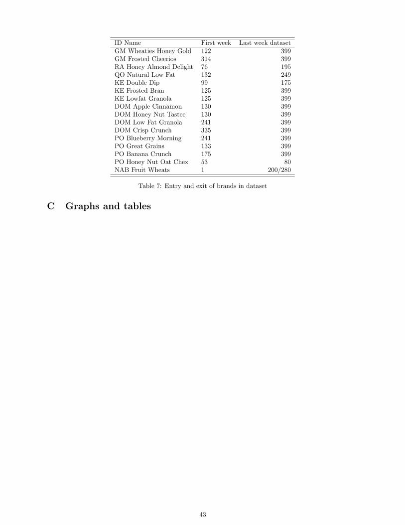
ID Name First week Last week datasetGM Wheaties Honey Gold 122 399GM Frosted Cheerios 314 399RA Honey Almond Delight 76 195QO Natural Low Fat 132 249KE Double Dip 99 175KE Frosted Bran 125 399KE Lowfat Granola 125 399DOM Apple Cinnamon 130 399DOM Honey Nut Tastee 130 399DOM Low Fat Granola 241 399DOM Crisp Crunch 335 399PO Blueberry Morning 241 399PO Great Grains 133 399PO Banana Crunch 175 399PO Honey Nut Oat Chex 53 80NAB Fruit Wheats 1 200/280
Table 7: Entry and exit of brands in dataset
C Graphs and tables
43

Brand Name 92Q3 % 92Q3-93Q1 93Q1 % 92Q3-93Q3 93Q3 % 92Q3-94Q1 94Q1NAB Orig Shred Wheat 0.188 0.091 0.205 0.056 0.199 0.074 0.202NAB Spoon Size Shrd Wheat 0.185 0.004 0.186 0.059 0.196 0.110 0.206PO Grape Nuts Cereal 0.147 -0.004 0.146 0.042 0.153 0.035 0.152PO Raisin Bran 0.158 0.000 0.159 0.155 0.183 0.256 0.199PO Honeycomb 0.225 0.061 0.239 0.067 0.240 0.118 0.251GM Raisin Nut Bran 0.195 0.014 0.198 0.079 0.211 0.057 0.206GM Apple-Cin Cheerios 0.221 -0.042 0.212 -0.058 0.209 -0.099 0.200GM Wheaties 0.194 -0.053 0.184 -0.024 0.189 -0.048 0.185GM Cheerios 0.224 -0.071 0.208 -0.033 0.217 -0.040 0.215GM Honey Nut Cheerios 0.215 -0.035 0.207 -0.085 0.196 -0.066 0.200GM Lucky Charms 0.244 -0.029 0.237 0.013 0.247 -0.004 0.243GM TOTAL Corn Flakes 0.269 0.013 0.273 -0.023 0.263 -0.093 0.244GM Trix 0.276 -0.020 0.271 0.022 0.282 -0.046 0.264KE Froot Loops 0.233 0.005 0.234 0.105 0.257 0.111 0.258KE Special K 0.237 0.036 0.245 0.027 0.243 0.072 0.254KE Frosted Flakes 0.165 0.046 0.173 0.085 0.179 0.197 0.198KE Corn Pops 0.230 0.014 0.234 0.010 0.233 0.018 0.234KE Raisin Bran 0.160 0.021 0.163 0.105 0.177 0.142 0.182KE Corn Flakes 0.118 0.079 0.128 0.065 0.126 0.291 0.153KE Smacks 0.200 0.018 0.203 0.099 0.219 0.127 0.225KE Crispix 0.226 0.050 0.237 0.097 0.247 0.112 0.251KE JUST RIGHT FruitNut 0.177 0.041 0.185 0.150 0.204 0.150 0.204KE Nutri Grain 0.194 -0.005 0.193 0.113 0.216 0.125 0.219RA Corn Chex 0.236 0.013 0.239 0.058 0.249 0.159 0.273RA Wheat Chex 0.177 0.011 0.179 0.050 0.186 0.149 0.203RA Rice Chex 0.233 0.023 0.239 0.069 0.249 0.170 0.273QO 100% Natural Cereal 0.144 -0.010 0.143 -0.042 0.138 0.038 0.150QO Cap’n Crunch 0.195 0.043 0.204 0.084 0.212 0.108 0.217DOM Raisin Bran 0.115 0.036 0.119 0.021 0.117 -0.078 0.106DOM Crispy Rice 0.137 0.034 0.141 -0.056 0.129 0.032 0.141DOM Corn Flakes 0.076 -0.006 0.076 -0.072 0.071 0.121 0.085
Table 8: Post merger price changes
Figure 9: Average industry-wide retail margins over time – OLD VERSION
44

Quarter General Mills Ralston Post Kelloggs Nabisco Quaker Oats Dominicks
1 14.5 18.6 13.0 15.2 14.1 15.9 28.12 14.3 20.4 12.7 15.1 12.3 17.0 31.83 15.6 31.6 13.8 15.3 13.4 14.7 30.84 14.6 14.3 13.9 13.8 14.5 24.2 24.65 14.2 15.8 15.4 13.5 14.8 19.7 32.26 15.0 19.5 17.6 14.0 13.4 15.1 30.97 14.4 25.5 15.0 13.8 24.3 20.6 31.58 13.8 16.9 14.9 12.9 11.9 16.2 29.99 14.3 17.2 15.0 11.8 11.0 15.2 31.9
10 12.6 21.4 11.1 3.2 9.5 10.9 29.311 2.7 16.5 7.2 13.2 0.4 28.212 0.7 13.2 3.4 11.1 10.1 28.013 2.7 8.0 6.8 12.7 2.9 33.614 7.1 13.8 0.7 14.4 -9.7 26.315 19.6 24.0 19.6 19.7 23.0 31.016 13.4 39.8 18.1 21.0 20.8 33.017 18.0 19.3 9.8 18.8 24.9 34.918 18.9 24.9 17.5 19.9 22.8 38.320 18.0 18.5 15.5 21.7 16.4 34.821 13.5 28.5 15.9 16.9 10.7 49.722 16.2 20.0 16.7 16.3 13.2 42.423 14.1 21.1 16.1 19.7 11.7 34.724 15.2 22.3 15.6 20.4 19.4 42.025 19.8 23.5 19.5 19.3 16.1 42.626 24.6 29.5 24.3 20.2 22.7 42.727 24.3 28.6 19.0 34.2 39.4
Total 14.1 20.5 14.1 15.8 14.4 15.1 33.7
Table 9: Retail margin over time
quarter Sugar Transp. Employ Vit Oat Earn. Milling Cornsweet Packag. Commodi, fuels Gas Wheat
1 119.1 118.3 26.0 134.1 150.0 13.3 120.2 128.1 112.8 122.9 116.4 108.4 118.3 326.82 118.4 125.1 25.7 136.1 127.5 13.3 115.0 115.5 115.4 125.8 100.4 122.4 125.1 278.03 120.1 121.7 24.8 135.7 120.0 13.2 116.3 115.0 118.4 125.7 109.9 105.6 121.7 270.54 120.5 120.5 24.7 137.8 132.0 13.4 120.7 124.0 118.4 126.8 112.0 104.4 120.5 302.55 120.6 120.5 24.7 141.3 122.0 13.6 124.8 133.3 118.7 126.1 115.6 104.7 120.5 287.56 118.5 121.9 24.3 140.9 137.0 13.7 122.1 124.7 117.9 126.7 109.1 102.1 121.9 344.57 120.7 121.1 23.6 141.8 152.6 13.8 122.8 124.7 118.7 126.5 112.2 94.6 121.1 419.08 120.5 122.7 23.8 142.3 160.5 14.2 121.9 126.7 118.8 128.7 113.1 100.4 122.7 431.09 120.7 123.0 24.3 142.6 149.5 14.2 122.1 130.2 119.5 129.8 114.9 101.4 123.0 364.5
10 119.6 125.8 23.7 142.8 148.5 14.0 111.5 110.2 119.6 130.3 113.8 103.5 125.8 366.511 121.8 124.9 23.1 143.1 163.9 14.1 110.1 107.4 120.7 130.9 117.0 97.9 124.9 372.012 121.4 126.8 23.6 143.1 162.0 14.4 110.0 109.2 121.5 132.8 121.0 102.0 126.8 374.813 121.9 125.9 24.1 143.7 160.0 14.4 118.7 124.7 122.8 132.5 125.5 96.5 125.9 309.514 121.7 127.1 23.8 143.7 152.3 14.2 121.0 124.9 128.9 133.1 115.3 95.7 127.1 323.315 123.8 126.4 23.5 143.2 159.1 14.3 128.1 130.0 129.3 133.5 111.8 92.6 126.4 398.016 123.8 128.8 23.3 144.1 154.5 14.4 135.8 143.5 129.5 134.2 111.3 98.6 128.8 345.017 124.4 132.9 23.7 143.1 136.5 14.8 136.1 144.9 129.5 135.8 110.7 108.1 132.9 339.318 123.5 133.1 24.1 140.9 157.6 14.9 124.6 126.0 130.8 135.9 109.7 104.1 133.1 415.020 126.1 136.4 23.9 143.0 164.3 15.1 124.8 127.6 134.3 137.3 112.3 104.8 136.4 378.321 127.8 135.4 24.3 143.1 190.3 15.3 125.2 127.5 134.4 136.8 113.7 102.5 135.4 498.822 128.2 135.0 24.6 143.1 210.0 15.5 128.2 127.4 134.3 136.9 110.8 97.5 135.0 508.023 131.0 136.9 23.8 143.8 262.3 15.2 129.6 123.3 135.0 137.9 114.7 101.3 136.9 549.024 132.4 141.1 23.8 143.7 269.5 15.4 133.4 122.3 135.4 139.0 119.5 112.4 141.1 582.525 134.2 139.8 24.0 143.7 271.5 15.9 134.7 123.5 135.6 138.5 124.6 107.9 139.8 562.326 132.7 141.9 24.2 143.9 195.5 16.3 133.4 129.2 136.8 140.4 122.9 111.1 141.9 473.027 134.8 141.8 24.3 143.9 195.5 16.0 128.3 124.4 137.7 140.8 130.0 109.1 141.8 449.8
Total 123.8 128.4 24.1 141.8 169.0 14.4 123.5 124.7 125.3 132.1 114.7 103.2 128.4 394.0
Table 10: Cost Variation over time
45

Adult enhanced Adult simple Family Kids
PO Raisin Bran NAB Original Shredded Wheat GM Wheaties PO HoneycombGM Raisin Nut Bran NAB Spoon Size Shredded Wheat GM Cheerios GM Apple-Cinnamon CheeriosKE Raisin Bran PO Grape Nuts Cereal KE Corn Flakes GM Honey Nut CheeriosKE Nutri Grain GM TOTAL Corn Flakes KE Crispix GM Lucky CharmsQO 100% Natural Cereal KE Special K RA Corn Chex GM Trix
KE JUST RIGHT Fruit Nut RA Wheat Chex KE Froot LoopsRA Rice Chex KE Frosted Flakes
KE Corn PopsKE SmacksQO Cap’n Crunch
Table 11: Product segmentation
Variable Mean Std. Dev. Interaction Interaction Interaction InteractionSmall Child Income household size std. income
price -16.47 .79 8.2 -.91 – 67.34(2.49) (3.05) (41.55) (7.31) – (30.64)
const -12.03 -.02422 -1.19 – 1.49 –(.21) (.83) (10.52) – (3.94) –
sugar 2.16 -.01 -.34 – -.03 –(.21) (3.30) (3.73) – (6.08) –
mushy -.01 .03 -.01 – -.01 –(.10) (.02) (.08) – (.14) –
Table 12: Demand side estimates for Random Coefficient Logit model
Figure 10: Average weekly prices per brand over time
46

Figure 11: Scatterplot average weekly prices
Figure 12: Quadratic fit of brand-specific prices over time
47

Figure 13: Quadratic fit of average firm-prices over time
Figure 14: Average industry-wide prices over time - including and excluding promotions
48
References
Bresnahan, T. (1982): “The oligopoly solution concept is identified,” Economics Letters,
10(1-2), 87–92.
(1987): “Competition and collusion in the American automobile industry: The 1955
price war,” The Journal of Industrial Economics, pp. 457–482.
(1989): “Empirical studies of industries with market power,” Handbook of industrial
organization, 2, 1011–1057.
Ciliberto, F., and J. Williams (2010): “Does Multimarket Contact Facilitate Tacit Col-
lusion? Inference on Conjectural Parameters in the Airline Industry,” .
Corts, K. (1995): The ready-to-eat breakfast cereal industry in 1994 (A). Harvard Business
School.
(1999): “Conduct parameters and the measurement of market power,” Journal of
Econometrics, 88(2), 227–250.
Farrell, J., and C. Shapiro (1990): “Horizontal mergers: An equilibrium analysis,” The
American Economic Review, pp. 107–126.
Feenstra, R., and J. Levinsohn (1995): “Estimating markups and market conduct with
multidimensional product attributes,” The Review of Economic Studies, 62(1), 19.
Gasmi, F., J. Laffont, and Q. Vuong (1992): “Econometric Analysisof Collusive Behav-
iorin a Soft-Drink Market,” Journal of Economics & Management Strategy, 1(2), 277–311.
Genesove, D., and W. Mullin (1998): “Testing static oligopoly models: conduct and cost
in the sugar industry, 1890-1914,” The Rand Journal of Economics, 29(2), 355–377.
Hausman, J. (1996): “Valuation of new goods under perfect and imperfect competition,”
Chicago: National Bureau of Economic Research.
Hitsch, G. (2006): “An empirical model of optimal dynamic product launch and exit under
demand uncertainty,” Marketing Science, pp. 25–50.
Lau, L. (1982): “On identifying the degree of competitiveness from industry price and
output data,” Economics Letters, 10(1-2), 93–99.
Nevo, A. (1998): “Identification of the oligopoly solution concept in a differentiated-
products industry,” Economics Letters, 59(3), 391–395.
(2000): “Mergers with differentiated products: The case of the ready-to-eat cereal
industry,” The RAND Journal of Economics, pp. 395–421.
(2001): “Measuring Market Power in the Ready-to-Eat Cereal Industry,” Econo-
metrica, 69(2), 307–342.
49

Nocke, V., and M. Whinston (2010): “Dynamic Merger Review,” Journal of Political
Economy, 118(6), 1201–1251.
Oliveira, A. (2011): “Estimating market Power with a Generalized Supply Relation: Ap-
plication to an Airline Antitrust Case,” .
Orcholski, T. (2010): “?Identifying collusion in the airline industry,” Unpublished working
paper.
Rivers, D., and Q. Vuong (2002): “Model selection tests for nonlinear dynamic models,”
The Econometrics Journal, 5(1), 1–39.
Rubinfeld, D. (2000): “Market definition with differentiated products: the post/Nabisco
cereal Merger,” Antitrust Law Journal, 68, 163.
Schmalensee, R. (1978): “Entry deterrence in the ready-to-eat breakfast cereal industry,”
The Bell Journal of Economics, pp. 305–327.
Vuong, Q. (1989): “Likelihood ratio tests for model selection and non-nested hypotheses,”
Econometrica, 57(2), 307–333.
Weinberg, M., and D. Hosken (2009): “Using Mergers to Test a Model of Oligopoly,”
mimeo.
Yoshimoto, H. (2011): “Reliability Examination in Horizontal-Merger Price Simulations:
An Ex-Post Evaluation of the Gap between Predicted and Observed Prices in the 1998
Hyundai–Kia Merger,” .
50