conduct and precision of bond grindability testing

~ p,,. .... n Minerais Engineering, Vol. 14, No. 10, pp. 1187-1197,2001

© 200! Elsevier Science Ltd Ali rights reserved

0892-6875(Ol)OO13~ 0892-6875/01/$ - see front matter

CONDUCT AND PRECISION OF BOND GRINDABILITY TESTING*

J.B. MOSHER and C.B. TAGUE

A.R. MacPherson Consultants Ltd., 4601 Indiana St., Golden, CO 80403, USA E-mail: [email protected]

(Received 25 April 2001 ; accepted 26 July 2001)

ABSTRACT

Evaluating the comminution energy requirements of ores using traditional Bond work index testing is well established; su ch testing is conducted on essentiaUy aU development properties, and is widely used as a benchmarkfor plant performance. Use of the Bond tests to describe ore hardness is so widespread that Bond work indices are often discussed as an ore property. ln spite ofwidespread use for over 70 years, there is often great confusion about how to conduct Bond tests accurately and precisely. Round-robin testing between laboratories often reveals variations in procedures, and makes assessment of test accuracy difficult. This paper details test methodology and procedural closing criteria for conducting Bond tests, discusses precision of test series conducted in a single laboratory with a single procedure, and details typical pitfaUs encountered in testing. @ 2001 Elsevier Science Ltd. AU rights reserved.

Keywords Comminution; crushing; grinding; mineraI processing

INTRODUCTION

ln large cornrninution circuits designed today, aB-inclusive safety factors can range from 15 to 40%, depending on a variety of factors including expansion plans, ore variability, and the project's capital cost sensitivity. In theory, the safety factor should aBow maintaining design production under aB conditions of liner life, during operation at less than optimum power efficiency (whether intentional or not), and over a specified range of ore hardness. Of course, relatively little of the safety factor should be required to account for inaccurate or imprecise ore characterization.

Bond testing has been in use since the late 1920's; laboratories and operations around world use the procedure as a component of comminution circuit design and to evaluate plant performance. In spite of such long-standing use, the topic of accuracy and precision of Bond work index determinations recurs with great frequency.

• Presented at Comminution '01, Brisbane, Australia, March 2001

1187

1188 J. B. Mosher and C. B. Tague

In conjunction with ore characterization for Newcrest's Cadia Hill project, a paper was published concerning the reproducibility (in different laboratories) and repeatability (indicating repeat tests within the same lab) of various ore breakage and grindability tests, including the Bond rod and ball mill tests (Angove and Dunne, 1997). That study focused on test reproducibility, and indicated differences (between maximum and minimum values) for Bond bail mill work indices of 4 to 13 %, and 8 to 31 % for rod mill work indices. Angove and Dunne concluded that the Bond procedures "appeared relatively robust," and that reproducibility could be improved if laboratories followed "accepted best practices" in conducting tests.

This paper addresses the precision (repeatability) of Bond ball and rod mill tests (variability independent of sampling or procedural variation) and recommends procedural guide1ines that have proven to be successful in numerous internai and external QAJQC programs. In addressing these issues, this paper will briefly discuss the background of the Bond grindability tests, discuss test sensitivity in terms of the measured variables, detail test procedures designed to maximize the accuracy and precision of the test, and present results of repeatability test series conducted using these procedures.

BACKGROUND

Prior to discussing the accuracy and precision of Bond tests, a recap of the development of the Bond tests is in order. Fred C. Bond observed that batch-grinding tests were inadequate to establish the energy requirement for milling ores. He noted that batch tests could result in inaccurate prediction of grinding energy requirements, particularly for closed circuit grinding, or for ores with multiple rock or minerai types. Based on his observations, Bond and others at Allis-Chaimers deve10ped a locked cycle ball mill test that allowed a determination of the energy requirement to mill ore at steady state conditions, with an equilibrium circulating load. After conducting these tests at Allis-Chalmers in the late 1920' s, the procedure was published in 1933 (Maxson et al, 1933).

The ball mill test has remained largely unchanged except for refinements in data analyses, and Bond subsequently developed an analogous locked cycle rod mill test. With these tests as the basis for ore characterization, Bond continued to develop a methodology for interpreting test results and how they could be used to predict grinding energy requirements. These efforts culminated in Bond's development of the ''Third Theory" (Bond, 1952). According to Bond, the first theory was Rittenger's, and the second was Kick's. Bond continued development of equations to calculate Bond work indices, and made the final revisions ofthese equations in 1961; these equations have been extensively used since (Bond, 1961).

Despite Bond's best efforts to define the ball mill work index as first principles-based determination of the amount of energy "required to reduce from infinite size to 80 pct passing 100 mesh," based on crack length, most regard the Bond test as empirical. Regardless, the Bond indices and subsequent calculations for energy requirements have proven themselves to be remarkably reliable as a prediction of energy requirements in commercially sized mills. As such, the Bond test and calculations are tremendously useful in sizing and analyzing comminution circuits.

Bond testing is a standard part of ore characterization for comminution circuit design and analyses. The question of Bond repeatability often arises, along with discussions about the source of discrepancies between laboratories. Due to insufficient knowledge concerning the basic repeatability of the Bond tests, and inconsistent procedures from lab to lab, the se discussions occur far too often. This paper endeavors to address the repeatability of the Bond grindability tests, the proper conduct of experiments to minimize error, and provide a basis for comparison for Bond results.

Prior to addressing test sensitivity and repeatability, it is useful to examine the range of Bond test results. Figure 1 presents the results of Bond bail mill work index (BW j ) determinations conducted at A.R. MacPherson's Golden, Colorado location over the past several years. While the 1000-odd tests in Figure 1 cannot be categorically called representative of all mill feeds, it is an adequate number to provide a reasonable representation of Bond work index values for typical ores. The standard deviation (SD) of these results is 3.6 kWh/mt. Figure 2 presents the results of approximately 700 Bond rod mill work index (RWi )

determinations over the same period. (The rod mill tests are not exclusively a subset of the bail mill tests,

Conduct and precision of bond grindability testing 1189

and are therefore plotted separately). The SD of the rod mill results is 3.8 kWh/mt. For both Figures 1 and 2, the x-axis is labeled in 0.5 SD increments.

;...

250 .----------------------------------------------,

Mean = 14.6 kWh/ml 200 Median = 14.8 kWh/ml

50

o 7.4 9.2 11.0 12.8 14.6 16.4 18.2 20.0 21.8

BW i , kWh/mt

Fig.l Histogram of Bond bail mill work index results.

160,--------------------------------------, Mean = 14.8 kWh/ml

140 Median = 14.8 kWh/ml

120

::; 100 e.;

5- 80 e.; ... ~ 60

40

20

o 7.2 9.1 11.0 129 14.8 16.7 18.6 20.5 22.3

RW i • kWh/mt

Fig.2 Histogram of Bond rod mill work index results.

TEST SENSITIVITY

The Bond equations for calculating work indices are weil known, and presented in Equation la and lb (Bond, 1961).

49.1 BWj (kWh/mt) = -----,.---------,-

P O.23 G 0.82 [10 10 J x pr X ---- - ----

1 ~P80 ~F80

(la)


RWi (kWh/mt) 68.4

(lb)

3 [10 10) PIO.2. X GprO.625

x ~Pso - ~Fso

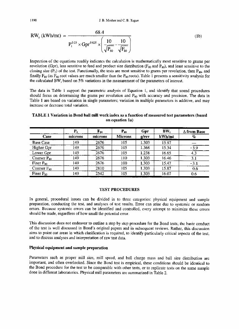
Inspection of the equations readily indicates the calculation is mathematically most sensitive to grams per revolution (Gpr), less sensitive to feed and product size distribution (Fso and Pso), and least sensitive to the closing size (Pl) of the test. Functionally, the tests are most sensitive to grams per revolution, then Pso, and finally Fso (as Fso root values are much smaller than the Psoroots). Table 1 presents a sensitivity analysis for the calculated BW j based on 5% variations in the measurement of the parameters of interest.

The data in Table 1 support the parametric analysis of Equation 1, and identify that sound procedures should focus on determining the grams per revolution and Pso with accuracy and precision. The data in Table 1 are based on variation in single parameters; variation in multiple parameters is additive, and may increase or decrease total variation.

TABLE 1 Variation in Bond bail mill work index as a function of measured test parameters (based on equation la)

Pl Fso Pso Gpr BW j Afrom Base Case microns microns Microns g/rev kWh/mt %

Base Case 149 2676 105 1.303 15.97 -

Higher Gpr 149 2676 105 1.368 15.34 -3.9 LowerGpr 149 2676 105 1.238 16.65 4.3 Coarser Pso 149 2676 110 1.303 16.46 3.1 Finer Pso 149 2676 100 1.303 15.47 -3.1 Coarser Fso 149 2810 105 1.303 15.87 -0.6 Finer Fso 149 2542 105 1.303 16.07 0.6

TEST PROCEDURES

In general, procedural issues can be divided in to three categories: physical equipment and sample preparation, conducting the test, and analyses of test results. Error can arise due to systemic or random errors. Because systemic errors can be identified and controlled, every attempt to minimize these errors should be made, regardless of how small the potential error.

This discussion does not endeavor to outline a step by step procedure for the Bond tests; the basic conduct of the test is weil discussed in Bond's original papers and in subsequent reviews. Rather, this discussion ai ms to point out areas in which clarification is required, to identify particularly critical aspects of the test, and to discuss analyses and interpretation of raw test data.

Physical equipment and sample preparation

Parameters such as proper mill size, mill speed, and bail charge mass and bail size distribution are important, and often overlooked. Since the Bond test is empirical, these conditions should be identical to the Bond procedure for the test to be comparable with other tests, or to replicate tests on the same sample do ne in different laboratories. Physical mill parameters are summarized in Table 2.


TABLE 2 Summary of physical Bond mill parameters

Bali Mill Rod Mill

Mill Size (D x L, cm) 30.48 by 30.48 30.48 by 60.96 Mill Speed (rpm) 70 46 Media Charge (g) 21,125 33,380 Liner Type Smooth Wave

The Bond baIl mill steel charge is often a source of discussion and consternation. There is little doubt, and in fact Bond conceded, that the Bond specified bail charge for the test is not likely the optimum charge. The charge could be optimized depending on the sample and the grind size, but this does little to contribute to standard conditions. Once one accepts that a standard charge should be used, there is often confusion over the appropriate standard. This is not surprising considering the several factors.

Pirst, Bond quoted non-standard size balls in specifying his recipe. As a result, many efforts to duplicate Bond's charge are thwarted by the inability to find balls of the appropriate size. Secondly, the widely quoted Minerais Processing Handbook (MPH) incorrectly specifies Bond's recipe (Bergstrom 1985). The MPH specifies baIl size, bail quantity per fraction, and mass of each fraction. Unfortunately, the indicated baIl size and baIl number are inconsistent with the bail mass per size fraction. The MPH also incorrectly specifies 0.5 inch balls (instead of 0.61 inch balls) for the fine st bail size. Finally, the supplier of Bond mills (Bico-Braun) specifies a charge drastically different from the original. While Bico's specified charge uses standard baIl sizes, the weight distribution of bail sizes is significantly different than Bond's, and baIl sizes are coarser across the entire size range.

In addition to being in conflict with Bond's published bail charge, neither the MPH nor the Bico-Braun charges are internally consistent as far as specified bail size and indicated charge mass. Only Bond's charge is consistent with his specified charge mass and surface area. Therefore, on the se bases, when this paper specifies the Bond bail charge, it references Bond' s published charge (Bond, 1961).

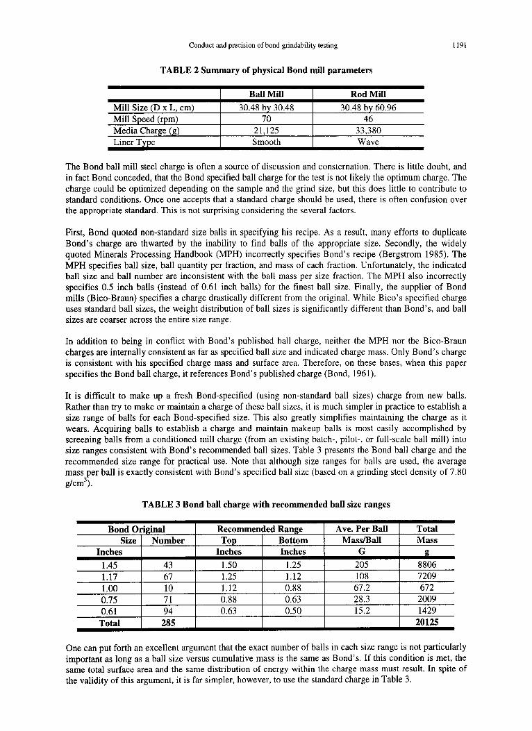
It is difficult to make up a fresh Bond-specified (using non-standard baIl sizes) charge from new balls. Rather than try to make or maintain a charge of these bail sizes, it is much simpler in practice to establish a size range of balls for each Bond-specified size. This also greatly simplifies maintaining the charge as it wears. Acquiring balls to establish a charge and maintain makeup balls is most easily accomplished by screening balls from a conditioned mill charge (from an existing batch-, pilot-, or full-scale bail mill) into size ranges consistent with Bond's recommended bail sizes. Table 3 presents the Bond bail charge and the recommended size range for practical use. Note that although size ranges for balls are used, the average mass per bail is exactly consistent with Bond's specified bail size (based on a grinding steel density of7.80 g/cm3

).

TABLE 3 Bond bail charge with recommended bail size ranges

Bond Original Recommended Range Ave. Per Bali Total Size Number Top BoUom MasslBall Mass

Inches Inches Inches G g

1.45 43 1.50 1.25 205 8806 1.17 67 1.25 1.12 108 7209 1.00 10 1.12 0.88 67.2 672 0.75 71 0.88 0.63 28.3 2009 0.61 94 0.63 0.50 15.2 1429

Total 285 20125

One can put forth an excellent argument that the exact number of balls in each size range is not particularly important as long as a ball size versus cumulative mass is the same as Bond's. If this condition is met, the same total surface area and the same distribution of energy within the charge mass must result. In spite of the validity ofthis argument, it is far simpler, however, to use the standard charge in Table 3.


Analysis of the data in Table 3 indicates that the geometric me an of the size ranges provided does not exactly correspond with the mean size required for the mean mass per baIl. Screen sizes were selected such that commonly available screens were used, and having balls within each size range skewed slightly towards either the top or bottom screen is of no practical consequence as long as the total mass per fraction requirement is met.

The Bond baIl charge requires maintenance. Checking the baIl charge every ten tests is a practical approach, with the ball charge reconstituted when any size fraction is off by more 10 grams, or the total charge off by more than 10 grams. While this sounds time consuming, it can be quite efficient if bins of balls in the appropriate size range are maintained. After counting out the appropriate number of balls, balls within the size range are swapped back and forth until the appropriate weight is obtained.

Constant volume of feed from test to test is important. In order to ensure constant volume of the initial feed sample, mechanical tamping (on a vibrating pad for example) is more repeatable than hand tamping. Prior to starting the test, make-up feed for each cycle should be mechanically split. Finally, test feed should be carefully stage-crushed, and should not be scalped of fines generated in stage crushing. For convenience, Bond adopted the 80% passing size to describe feed and product size distributions, but recognized limitations when the log-log slope of the feed and product differed.

When preparing feed splits for each cycle, mechanical splitting should be employed. Prior to starting the test, it is convenient to mechanically split the test feed into eighths (preferably using a rotary splitter). When splitting out the exact make-up feed amount for each cycle's (to replace the fraction removed as final product), feed should be mechanically split (to ±1O grams) instead of "scoop sampled". Riffle splitters are the most convenient device for this splitting step.

Test conduct and closure

The parametric analysis indicated that the most important parameters for caJculating the work indices are the amount of final product produced per mill revolution (Gpr) and the product size distribution, as described by the 80% passing size (Pso). Therefore, procedures focused on maximizing repeatability should focus on definition of when a test is at steady state, and the size distribution of the product at those conditions.

Essentially, conducting a Bond work index test is analogous to a locked cycle flotation test, or any other locked-cycle test. Implicit in conducting locked-cycle tests is developing a steady state condition. In conducting locked-cycle tests, care must be taken to ensure that material added to each cycle (after removing product sized material) is weil blended and representative of the bulk sample. Mechanical methods are the best way to ensure that splitting errors do not occur. To determine the correct amount of ore to add, the screening procedure must have safeguards to ensure complete screening between cycles.

One of the most important steps in conducting a locked-cycle test is deciding when the test is at steadystate. For Bond testing, test closure should include a maximum deviation from the highest and lowest Gpr (suggested value of 3%) and a reversaI in the rate of mill production during last three cycles (failure to reverse indicates instability). A final criterion, a minimum number of cycles (with the suggested number of seven), is arbitrary but ensures that enough mill volumes are processed to provide a reasonable assurance of steady state. Together, these three criteria ensure accurate, repeatable test closure. Figure 3 depicts data from two typical properly closed Bond baIl mill work index tests. One test (average Gpr of 1.412 grams) closes to within of 1.1 % (between the highest and lowest Gpr values), and the second test (average Gpr of 1.610 grams) closes to within 0.6%.

Con du ct and precision of bond grindability testing 1193

1.75 ....... Cycle )-7 A\'cr.g~~

1.65 --Cycle )-7 Aver.ge = 1.61 g

1.55 /-

" .. Co ~

/

el) /

145

1.35

1.25 0 2 4 6 8

Cycles

Fig.3 Typical properly closed Bond bail mill work index test data.

Figure 4 presents an example of a very poorly closed rod mill work index test. While the last three cycles show a reversai in quantity of product generated, and the test has been fUn at least seven cycles, there is still greater th an a 10% difference between the highest and lowest Gpr values in the last three cycles. The Bond rod mill work index that results from the average value plotted in Figure 3 is 14.0 kWh/mt, but ranges from 13.1 to 14.8 kWh/mt for the highest and lowest Gpr of the last three cycles, respectively. This level of imprecision is obviously less than satisfactory.

14.0 • 13.0 • •

• • 12.0 ................ -- ..

~ 11.0 6j) • • 10.0

9.0 • f ----... A verage, Cycles 8-10

8.0

0 2 3 4 5 6 7 8 9 10

Cycles

Fig.4 Improperly closed Bond rod mill work index data.

Figure 5 presents data for a Bond bail mill test that iIIustrates the importance of proper selection of the correct test closure point. For this test, production of ground product (Gpr) shows a reversai for cycles 5-7, but with a difference of approximately 6% between the highest and lowest Gpr. After running the test for another four cycles, the Gpr again reverses, this time to within 3%. The test closure at this point differs from the cycle 5-7 closure. The change suggests that steady state had not yet been reached in cycles 5-7. Such a result can imply that the composition of the recycle load was important for determining steady state grinding rate, or that a splitting/sampling error was made in adding new feed. The bail mill work index calculated from cycles 5-7 is 24.5 kWh/mt, versus 25.8 kWh/mt for cycles 9-11 (a difference of approximately 5%).

1.00 ,--------------------, <)

0_90 <)

... 0.80 - - - - _ .. _ .. ~ - - _.;; - - -'0' _. - 0- - _ ... - - - -0-' - --~ _ ..... -- _. -'. - -_ .... -

~ v

0.70

1

---_. _. Average, Cycles 5-7 1 0.60

--Average, Cycles 9-11 0.50 -l---.---,--.----.--.--.--=r=::,:==;:::==;:=:::;==--l

o 2 3 4 5 6 7 8 9 10 11 12

Cycles

Fig.5 Bond bail mill data showing the importance of steady state closure_

1194 J. B. Mosher and C. B. rague

After the test has been closed, and product from the test is collected, an accurate and repeatable Pso determination is required. Most laboratories screen the final product (screen undersize from the test closing size) on a standard root of 2 sieve series. This methodology can lead to sorne imprecision depending on the particle size distribution of the test product.

A histogram of PgO's for Bond tests closing at 149 microns is presented in Figure 6; the mean PgO is 117 microns. After screening the product at 149 microns, the next screen in the root of 2 series is a 105 micron screen. Extrapolating between these two screens is not a particularly rigorous way to define the shape of the particle size distribution around the Pso, particularly when the 149 micron screen merely defines the 100% passing point. A much better degree of accuracy in defining the Pso can be gained by the inclusion of a fourth root of 2 screen (125 microns) in the series.

Table 4 presents Bond baIl mill test product size distribution data from a gold ore with a slightly coarser than normal Pso. The left column calculates the Pso based on inclusion of a 125 micron screen in a standard root of two series and the spline method, while the right column calculates the PgO based on typical root of 2 screen series and linear regression.

140

120 Mean = Il 7 microns

Median = 118 microns , 100

.... ... 80 c .. ::1 r:r" 60 .. .. '"' 40

20

0

103 106 110 113 1\7 12\ 124 128 131

PSO' microns

Fig.6 Histogram of Pso' s for Bond bail mill tests closed at 149 !lm .

TABLE 4 Addition of a 4th root of 2 screen in particIe size analyses

Screen Retained Cumulative Passim!: Microns % %

149 100 100 125 75.6 -

105 64.5 64.5 74 46.8 46.8 53 33.5 33.5 37 24.7 24.7

-37 0 0.0 Pao 133 124

These data indicate that significant error can be introduced by linear regression from the 100% passing size to the first root 2 screen deck (105 microns) as compared with the inclusion of a 125 micron screen and the use of spline fitting. Based on the Pso's calculated from the data in Table 3, the Bond baIl mill work index changes from 14.8 to 15.5 kWh/mt (a difference of 4.2%) based solely on the inclusion of an additional sieve and the use of spline fitting to estimate the PgO size.


Differences between the two techniques range from zero to ten microns, with the greatest differences for samples with coarser Pso's (as more extrapolation from the 105 micron screen is required). This seemingly minor difference in analytical procedure can therefore result in a difference of up to 5% in the Bond bail mill work index. In general, inclusion of the 125 micron screen allows much better definition of the Pso, particularly for ores producing a somewhat coarser size distribution.

Similarly, for the rod mill test, inclusion of a 1.00 mm screen between 1.19 and 0.84 mm screens will produce more accurate results. Also, while computationally less important (as regards to the calculated work index value), it makes little sense not to follow like procedures for the Fso determination. For the bail mill test, this entails using a 2.83 mm screen between the 3.36 and 2.38 mm screens; for the rod mill test, an 11.2 mm screen is inserted between the 12.7 and 9.5 mm screens.

Typical laboratory practice is to combine the undersize product from the last three cycles. A split of this sample is then screened to determine the particle size. The sub-sample for screening should be mechanically split, then wet screened at the finest screen size, and the oversize dried and screened at coarser sizes. The screening procedure should include measures to ensure that screening is complete.

As a final note on product screening, it makes sense to examine the Pso in light of typical Pso's at the closing size employed. If the Pso determined is outside the normal range, screening the entire combined product of the last three cycles (instead of a split) will ensure that splitting does not introduce error. While careful mechanical splitting should not result in poor splits, mistakes can occur.

TEST REPEA TABILITY

To assess the repeatability of the Bond test, a series of ten rod mill and ten bail mill tests were conducted on splits of copper porphyry ore of moderate hardness. Samples for each test were rotary split after routine preparation to minus 12.7 and 3.36 mm (for the rod and bail mill tests, respectively). Without prior knowledge of a replicate test program, two different technicians collectively performed the test series. The series were conducted using MacPherson's standard procedures for Bond rod and bail mill tests; these procedures incorporate items discussed in the Test Procedures section.

The me an of the ten test bail mill work index determination series (obviously fewer than the statistical optimum) was 15.84 kWh/mt, with a SD of 0.28 kWh/mt. Thus, at two SDs, the range of the tests was ±3.5%. A histogram of test data is presented in Figure 7 (with the x-axis scaled in 0.5 SD increments). One test (resulting in the lowest BW j ) included an errant Pso and would have normally been flagged for repeatfreanalyses; for completeness in evaluating the standard procedure, this test was included in data analyses.

6

5

2

o

Mean = 15.84 kWh/ml

SD= 0.28 kWh/ml

15.28 15.42 15.56 15.70 15.84 15.98 16.12 16.25

BW1, kWh/mt

Fig.7 Histogram ofreplicate Bond bail mill series.


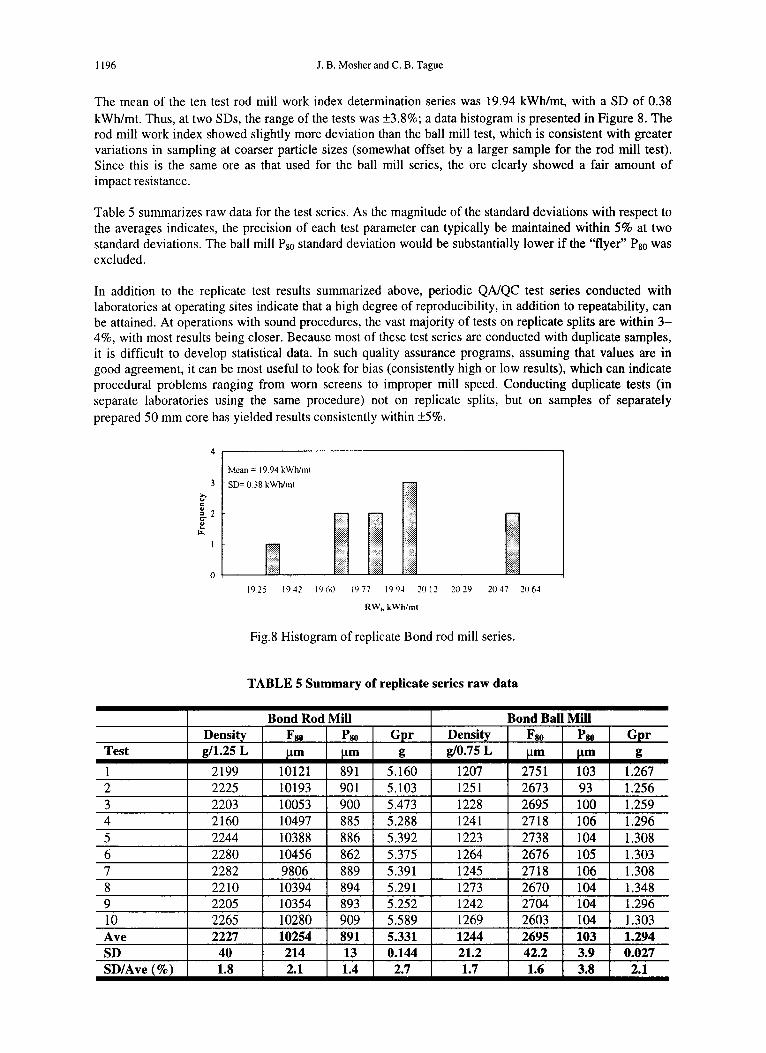
The me an of the ten test rod mill work index determination series was 19.94 kWh/mt, with a SD of 0.38 kWh/mt. Thus, at two SDs, the range of the tests was ±3.8%; a data histogram is presented in Figure 8. The rod mil! work index showed slightly more deviation than the ball mil! test, which is consistent with greater variations in sampling at coarser particle sizes (somewhat offset by a larger sample for the rod mill test). Since this is the same ore as that used for the ball mill series, the ore clearly showed a fair amount of impact resistance.

Table 5 summarizes raw data for the test series. As the magnitude of the standard deviations with respect to the averages indicates, the precision of each test parameter can typically be maintained within 5% at two standard deviations. The ball mil! PgO standard deviation would be substantially lower if the "flyer" PgO was excluded.

In addition to the replicate test results summarized above, periodic QAJQC test series conducted with laboratories at operating sites indicate that a high degree of reproducibility, in addition to repeatability, can be attained. At operations with sound procedures, the vast majority of tests on replicate splits are within 3-4%, with most results being closer. Because most of these test series are conducted with duplicate samples, it is difficult to develop statistical data. In such quality assurance programs, assuming that values are in good agreement, it can be most useful to look for bias (consistently high or low results), which can indicate procedural problems ranging from worn screens to improper mil! speed. Conducting duplicate tests (in separate laboratories using the same procedure) not on replicate splits, but on samples of separately prepared 50 mm core has yielded results consistently within ±5%.

4 ~----------------------------------------~

Mean = 19 94 kWh/ml

3 SD= 038 kWh/ml

o 1-------,-

1925 19.42 1960 1977 199~ 2012 2029 2047 2(J6~

RW" kWh/mi

Fig.8 Histogram of replicate Bond rod mil! series.

TABLE 5 Summary of replicate series raw data

Bond Rod Mill Bond BaIl Mill Density F80 Pao Gpr Density Fso P80 Gpr

Test g/1.25 L J,1m J,1m g g/0.75 L J,1m J,1m g

1 2199 10121 891 5.160 1207 2751 103 1.267 2 2225 10193 901 5.103 1251 2673 93 1.256 3 2203 10053 900 5.473 1228 2695 100 1.259 4 2160 10497 885 5.288 1241 2718 106 1.296 5 2244 10388 886 5.392 1223 2738 104 1.308 6 2280 10456 862 5.375 1264 2676 105 1.303 7 2282 9806 889 5.391 1245 2718 106 1.308 8 2210 10394 894 5.291 1273 2670 104 1.348 9 2205 10354 893 5.252 1242 2704 104 1.296 10 2265 10280 909 5.589 1269 2603 104 1.303 Ave 2227 10254 891 5.331 1244 2695 103 1.294 SD 40 214 13 0.144 21.2 42.2 3.9 0.027 SD/Ave (%) 1.8 2.1 1.4 2.7 1.7 1.6 3.8 2.1

Conduct and precision of bond gri ndabi lit y testing 1197

CONCLUSIONS

The most significant factors in repeatability between laboratories, given that tests are conducted under standard conditions on properly split and prepared samples, are c10sure criteria and method of product size distribution analyses. The c10sure criteria discussed in this paper are simple, and are essentially unchanged from the criteria that Bond first published nearly 70 years ago. Adopting slightly more rigorous laboratory procedures can significantly improve the precision of conducting these standard grindability tests.

ln general, the Bond tests are quite repeatable. Within one laboratory, both rod and ball mill tests showed repeatability of less than ±4% at two standard deviations. Reporting Bond work indices beyond 0.1 kWh/mt is not merited based on the precision of the test. The reproducibility of work index determination can be improved significantly by steps to ensure test c10sure and by accurate determination of the test feed and product size distribution.

Bond tests have limitations, and today represent only a part of comminution testing and analyses methodologies. Presently, researchers are developing advanced methods for computer simulation of comminution circuits. As important as the computational techniques used in analyses are accurate determinations of ore breakage/grindability characteristics. In determining these characteristics, methods must determine ore breakage characteristics in an environment that is applicable to that of commercial milling applications, use a sample mass appropriate to the top size to minimize sampling variability, and evaluate the effect of a range of breakage energies.

Using existing standardized tests to determine parameters for advanced simulation techniques offers several advantages. Using an existing test minimizes additional training and expenditure necessary for specific test development and allows design and circuit evaluation from conventional as weil as newer approaches. Finally, using existing methods offers test platforms that have already solved sampling, test procedure, and data analysis problems.

REFERENCES

Angove, I.E. and Dunne, R.e. A Review of Standard Physical Ore Property Determinations. Proceedings World Gold Conference (Singapore), September, 1997.

Bergstrom, B.H. Crushability and Grindability. In SME Minerais Processing Handbook, edited by N.L. Weiss. SME Inc., Littleton, 1985, pp. 30-65-68.

Bond, F.e. The Third Theory of Comminution. Mining Engineering, May, 1952, p. 484. Bond, Fe. Crushing and Grinding Calculations: Part l, British Chemical Engineering, Volume 6, 1960,

Revised J anuary 2, 1961. Maxson, W.L., Cadena, F. and Bond, Fe. Grindability of Various Ores. Transactions American Institute of

Mining and Metallurgical Engineers, Vol. 112, 1933, p. 130.

Correspondence on papers published In Minerais Engineering IS invited bye-mail to [email protected]

conduct and precision of bond grindability testing

Documents