conditional expectation functionsecon.ucsb.edu/~doug/241b/lectures/01 conditional expectation... ·...
TRANSCRIPT

Conditional Expectation FunctionsEconometrics II
Douglas G. Steigerwald
UC Santa Barbara
D. Steigerwald (UCSB) Expectation Functions 1 / 29
OverviewReference: B. Hansen Econometrics Chapters 1 and 2.0 - 2.8
most commonly applied econometrics toolI least-squares estimation (regression)
tool to estimateI approximate conditional mean of dependent variableI as a function of covariates (regressors)I (y , x1, . . . , xK ) :=
�y , xT�
data is observational not experimentalI causality is di¢ cult to infer
example - wagesI random variable before measurementI observed wages are outcomes of the random variableI underpins the application of statistics to economics
D. Steigerwald (UCSB) Expectation Functions 2 / 29
Distribution of Wages
probability distributionI F (u) = P (wage � u)
median - measure of location (central tendency)I If F is continuous, m uniquely solves F (m) = 1
2I Otherwise, m = inf
nu : F (u) � 1
2
oI not a linear operator, some calculations are trickyI robust to tail perturbations
nonparametric distribution estimate (following slide)I 50,742 full-time non-military wage earners March 2009 CPSI bm = $19.23
D. Steigerwald (UCSB) Expectation Functions 3 / 29

D. Steigerwald (UCSB) Expectation Functions 4 / 29

Quantiles
a useful way to summarize a probability distribution
for any α 2 (0, 1), the αth quantile isI If F is continuous, qα uniquely solves F (qα) = αI Otherwise, qα = inf fu : F (u) � αgI q0.5 = m
quantile function, qα, viewed as a function of α is the inverse of F
if α is represented in percentage terms (10% instead of .1), quantilesare referred to as percentiles
I q0.5 = m is called the 50th percentileI q0.9 is called the 90th percentile
D. Steigerwald (UCSB) Expectation Functions 5 / 29
Density of Wages
If F is di¤erentiable, density function exists
f (u) =dduF (u)
F (u) and f (u) contain the same information
density is easier to interpret visually
mean - measure of location (y denotes wage)I if F is continuous, µ := E (y) =
R ∞�∞ uf (u) du
I formal de�nition, 240A Lecture on Random Variables and DistributionsI linear operator, not robust
nonparametric density estimate (following slide)bµ = $23.90data are skew, 64% of workers earn less than bµD. Steigerwald (UCSB) Expectation Functions 6 / 29
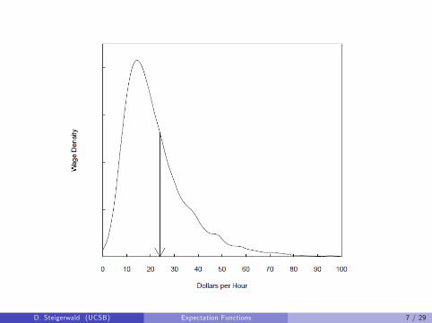
D. Steigerwald (UCSB) Expectation Functions 7 / 29
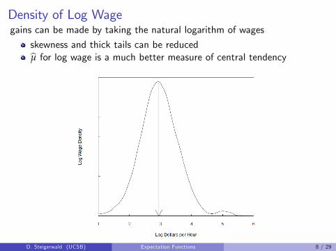
Density of Log Wagegains can be made by taking the natural logarithm of wages
skewness and thick tails can be reducedbµ for log wage is a much better measure of central tendency
D. Steigerwald (UCSB) Expectation Functions 8 / 29
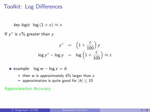
Toolkit: Log Di¤erences
key logic log (1+ x) � x
If y � is c% greater than y
y � =�1+
c100
�y
log y � � log y = log�1+
c100
�� c
example: logw � log z = bI then w is approximately b% larger than zI approximation is quite good for jbj � 10
Approximation Accuracy
D. Steigerwald (UCSB) Expectation Functions 9 / 29

Conditional ExpectationsIs the wage distribution the same for all workers?
Men versus women (43% of workers are women)I E (log (wage) jgender = man) = 3.05I E (log (wage) jgender = woman) = 2.81I 24% di¤erence in average wages between men and women
D. Steigerwald (UCSB) Expectation Functions 10 / 29
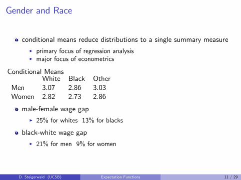
Gender and Race
conditional means reduce distributions to a single summary measureI primary focus of regression analysisI major focus of econometrics
Conditional MeansWhite Black Other
Men 3.07 2.86 3.03Women 2.82 2.73 2.86
male-female wage gapI 25% for whites 13% for blacks
black-white wage gapI 21% for men 9% for women
D. Steigerwald (UCSB) Expectation Functions 11 / 29

Education
after 9 years, conditional mean increases at a di¤erent ratemale-female gap is constant across education levels
I constant percentage di¤erence in wagesD. Steigerwald (UCSB) Expectation Functions 12 / 29
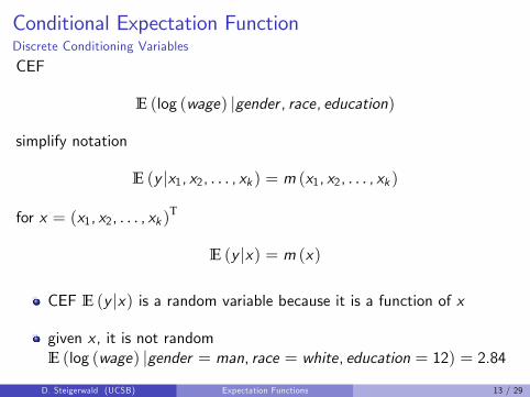
Conditional Expectation FunctionDiscrete Conditioning Variables
CEF
E (log (wage) jgender , race, education)
simplify notation
E (y jx1, x2, . . . , xk ) = m (x1, x2, . . . , xk )
for x = (x1, x2, . . . , xk )T
E (y jx) = m (x)
CEF E (y jx) is a random variable because it is a function of x
given x , it is not randomE (log (wage) jgender = man, race = white, education = 12) = 2.84
D. Steigerwald (UCSB) Expectation Functions 13 / 29
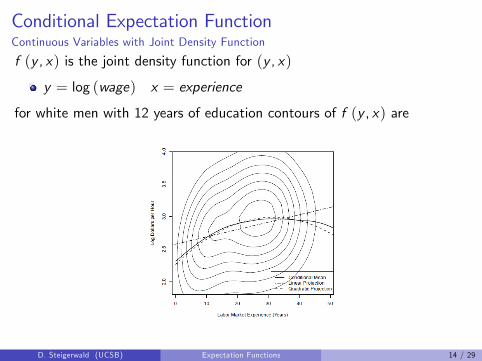
Conditional Expectation FunctionContinuous Variables with Joint Density Function
f (y , x) is the joint density function for (y , x)
y = log (wage) x = experience
for white men with 12 years of education contours of f (y , x) are
D. Steigerwald (UCSB) Expectation Functions 14 / 29

Conditional Densitya "slice" of the joint density contours yields the conditional density
shifts right and becomes more di¤use as experience increasesI little change as experience increases past 25 years
the conditional density is denoted fy jx (y jx) Conditional DensityD. Steigerwald (UCSB) Expectation Functions 15 / 29
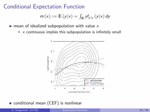
Conditional Expectation Function
m (x) := E (y jx) =R
Ryfy jx (y jx) dy
mean of idealized subpopulation with value xI x continuous implies this subpopulation is in�nitely small
conditional mean (CEF) is nonlinear
D. Steigerwald (UCSB) Expectation Functions 16 / 29

Toolkit: Law of Iterated Expectations
Simple Law
E (E (y jx)) = E (y) if E (y) < ∞
note E (E (y jx)) =R
RE (y jx) fx (x) dx
General Law (allows for 2 sets of conditioning variables)
E (E (y jx1, x2) jx1) = E (y jx1) if E (y) < ∞
"smaller information set wins"
D. Steigerwald (UCSB) Expectation Functions 17 / 29
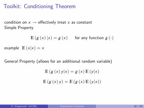
Toolkit: Conditioning Theorem
condition on x ! e¤ectively treat x as constantSimple Property
E (g (x) jx) = g (x) for any function g (�)
example E (x jx) = x
General Property (allows for an additional random variable)
E (g (x) y jx) = g (x)E (y jx)
E (g (x) y) = E (g (x)E (y jx))
D. Steigerwald (UCSB) Expectation Functions 18 / 29
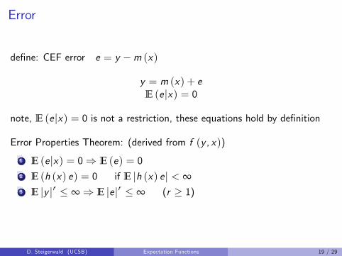
Error
de�ne: CEF error e = y �m (x)
y = m (x) + eE (ejx) = 0
note, E (ejx) = 0 is not a restriction, these equations hold by de�nition
Error Properties Theorem: (derived from f (y , x))
1 E (ejx) = 0) E (e) = 02 E (h (x) e) = 0 if E jh (x) ej < ∞3 E jy jr � ∞) E jejr � ∞ (r � 1)
D. Steigerwald (UCSB) Expectation Functions 19 / 29
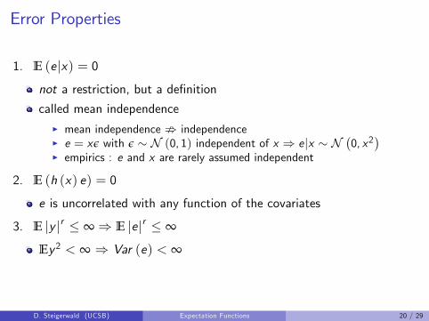
Error Properties
1. E (ejx) = 0not a restriction, but a de�nition
called mean independenceI mean independence ; independenceI e = xε with ε � N (0, 1) independent of x ) ejx � N
�0, x2
�I empirics : e and x are rarely assumed independent
2. E (h (x) e) = 0
e is uncorrelated with any function of the covariates
3. E jy jr � ∞) E jejr � ∞
Ey2 < ∞ ) Var (e) < ∞
D. Steigerwald (UCSB) Expectation Functions 20 / 29
Proofs
1 Proof of Simple LIE2 Proof of General LIE3 Proof of Conditioning Theorems4 Proof of Error Properties Theorem
D. Steigerwald (UCSB) Expectation Functions 21 / 29

Review
Implication of observational data?
causality is di¢ cult to infer
Should we model E (y jx) as linear in x?no
What are the key properties of e = y �E (y jx)?E (ejx) = 0 (by construction)
uncorrelated with any function of x
D. Steigerwald (UCSB) Expectation Functions 22 / 29
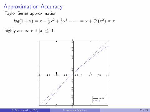
Approximation AccuracyTaylor Series approximation
log(1+ x) = x � 12x2 + 1
3x3 � � � � = x +O
�x2�� x
highly accurate if jx j � .1
D. Steigerwald (UCSB) Expectation Functions 23 / 29
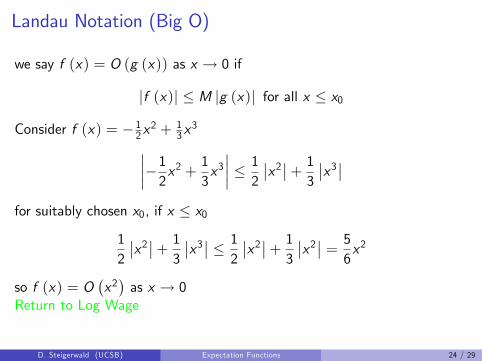
Landau Notation (Big O)
we say f (x) = O (g (x)) as x ! 0 if
jf (x)j � M jg (x)j for all x � x0
Consider f (x) = � 12x2 +13x3�����12x2 + 13x3
���� � 12
��x2��+ 13
��x3��for suitably chosen x0, if x � x0
12
��x2��+ 13
��x3�� � 12
��x2��+ 13
��x2�� = 56x2
so f (x) = O�x2�as x ! 0
Return to Log Wage
D. Steigerwald (UCSB) Expectation Functions 24 / 29
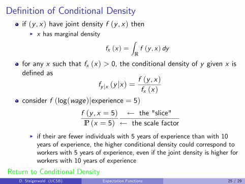
De�nition of Conditional Densityif (y , x) have joint density f (y , x) then
I x has marginal density
fx (x) =Z
Rf (y , x) dy
for any x such that fx (x) > 0, the conditional density of y given x isde�ned as
fy jx (y jx) =f (y , x)fx (x)
consider f (log(wage)jexperience = 5)f (y , x = 5)P (x = 5)
the "slice" the scale factor
I if their are fewer individuals with 5 years of experience than with 10years of experience, the higher conditional density could correspond toworkers with 5 years of experience, even if the joint density is higher forworkers with 10 years of experience
Return to Conditional DensityD. Steigerwald (UCSB) Expectation Functions 25 / 29
Proof of Simple Law of Iterated Expectations
Simple LIE: E (E (y jx)) = E (y)
assume (y , x) have joint density f (y , x) (for convenience)I E (y jx) is a function of the random variable x onlyI to calculate its expectation, integrate with respect to the density fx (x)of x
E (E (y jx)) =Z
RkE (y jx) fx (x) dx
I which equals (by substitution and by noting thatfy jx (y jx) fx (x) = f (y , x))Z
Rk
�ZRyfy jx (y jx) dy
�fx (x) dx =
ZRk
ZRyfy ,x (y , x) dydx
= E (y) ,
becauseR
Rk fy ,x (y , x) dx = fy (y). �
Return to Proofs
D. Steigerwald (UCSB) Expectation Functions 26 / 29
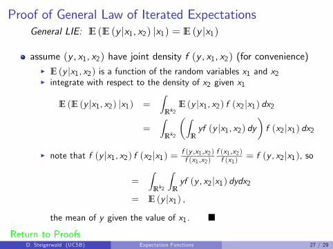
Proof of General Law of Iterated ExpectationsGeneral LIE: E (E (y jx1, x2) jx1) = E (y jx1)
assume (y , x1, x2) have joint density f (y , x1, x2) (for convenience)I E (y jx1, x2) is a function of the random variables x1 and x2I integrate with respect to the density of x2 given x1
E (E (y jx1, x2) jx1) =Z
Rk2E (y jx1, x2) f (x2 jx1) dx2
=Z
Rk2
�ZRyf (y jx1, x2) dy
�f (x2 jx1) dx2
I note that f (y jx1, x2) f (x2 jx1) = f (y ,x1,x2)f (x1,x2)
f (x1,x2)f (x1)
= f (y , x2 jx1), so
=Z
Rk2
ZRyf (y , x2 jx1) dydx2
= E (y jx1) ,
the mean of y given the value of x1. �Return to Proofs
D. Steigerwald (UCSB) Expectation Functions 27 / 29
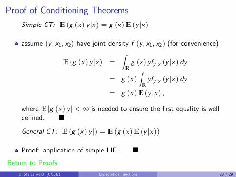
Proof of Conditioning Theorems
Simple CT: E (g (x) y jx) = g (x)E (y jx)
assume (y , x1, x2) have joint density f (y , x1, x2) (for convenience)
E (g (x) y jx) =Z
Rg (x) yfy jx (y jx) dy
= g (x)Z
Ryfy jx (y jx) dy
= g (x)E (y jx) ,
where E jg (x) y j < ∞ is needed to ensure the �rst equality is wellde�ned. �
General CT: E (g (x) y j) = E (g (x)E (y jx))
Proof: application of simple LIE. �Return to Proofs
D. Steigerwald (UCSB) Expectation Functions 28 / 29

Proof of Error Properties Theorem
Parts 1 and 2 follow trivially
Part 3: E jy jr � ∞) E jejr � ∞ (r � 1)
e = y �m (x)(E jejr )1/r
= (E jy �m (x)jr )1/r
I�E jy �m (x)jr
�1/r ��E jy jr
�1/r+�E jm (x)jr
�1/r (Minkowski�sInequality)
F E jE (y jx)jr � E jy jr for any r � 1 (Conditional ExpectationInequality)
I the two parts on the right are �nite by E jy jr � ∞
(E jejr )1/r � ∞ implies E jejr � ∞. �Return to Proofs
D. Steigerwald (UCSB) Expectation Functions 29 / 29