concrete models and empirical evaluations for the categorical compositional...

Concrete Models and Empirical Evaluationsfor the Categorical CompositionalDistributional Model of Meaning

Edward Grefenstette∗†Google DeepMind

Mehrnoosh Sadrzadeh∗∗†Queen Mary University of London

Modeling compositional meaning for sentences using empirical distributional methods has beena challenge for computational linguists. The categorical model of Clark, Coecke, and Sadrzadeh(2008) and Coecke, Sadrzadeh, and Clark (2010) provides a solution by unifying a categorialgrammar and a distributional model of meaning. It takes into account syntactic relationsduring semantic vector composition operations. But the setting is abstract: It has not beenevaluated on empirical data and applied to any language tasks. We generate concrete modelsfor this setting by developing algorithms to construct tensors and linear maps and instantiatethe abstract parameters using empirical data. We then evaluate our concrete models againstseveral experiments, both existing and new, based on measuring how well models align withhuman judgments in a paraphrase detection task. Our results show the implementation of thisgeneral abstract framework to perform on par with or outperform other leading models in theseexperiments.1

1. Introduction

The distributional approach to the semantic modeling of natural language, inspiredby the notion—presented by Firth (1957) and Harris (1968)—that the meaning of aword is tightly related to its context of use, has grown in popularity as a methodof semantic representation. It draws from the frequent use of vector-based documentmodels in information retrieval, modeling the meaning of words as vectors based onthe distribution of co-occurring terms within the context of a word.

Using various vector similarity metrics as a measure of semantic similarity, thesedistributional semantic models (DSMs) are used for a variety of NLP tasks, from

∗ DeepMind Technologies Ltd, 5 New Street Square, London EC4A 3 TW.E-mail: [email protected].

∗∗ School of Electronic Engineering and Computer Science, Queen Mary University of London, Mile EndRoad, London E1 4NS, United Kingdom. E-mail: [email protected].

† The work described in this article was performed while the authors were at the University of Oxford.1 Support from EPSRC grant EP/J002607/1 is acknowledged.

Submission received: 26 September 2012; revised submission received: 31 October 2013;accepted for publication: 5 April 2014.

doi:10.1162/COLI a 00209

© 2015 Association for Computational Linguistics

Computational Linguistics Volume 41, Number 1

automated thesaurus building (Grefenstette 1994; Curran 2004) to automated essaymarking (Landauer and Dumais 1997). The broader connection to information retrievaland its applications is also discussed by Manning, Raghavan, and Schutze (2011). Thesuccess of DSMs in essentially word-based tasks such as thesaurus extraction and con-struction (Grefenstette 1994; Curran 2004) invites an investigation into how DSMs canbe applied to NLP and information retrieval (IR) tasks revolving around larger units oftext, using semantic representations for phrases, sentences, or documents, constructedfrom lemma vectors. However, the problem of compositionality in DSMs—of how to gofrom word to sentence and beyond—has proved to be non-trivial.

A new framework, which we refer to as DisCoCat, initially presented in Clark,Coecke, and Sadrzadeh (2008) and Coecke, Sadrzadeh, and Clark (2010) reconcilesdistributional approaches to natural language semantics with the structured, logicalnature of formal semantic models. This framework is abstract; its theoretical predictionshave not been evaluated on real data, and its applications to empirical natural languageprocessing tasks have not been studied.

This article is the journal version of Grefenstette and Sadrzadeh (2011a, 2011b),which fill this gap in the DisCoCat literature; in it, we develop a concrete model andan unsupervised learning algorithm to instantiate the abstract vectors, linear maps, andvector spaces of the theoretical framework; we develop a series of empirical naturallanguage processing experiments and data sets and implement our algorithm on largescale real data; we analyze the outputs of the algorithm in terms of linear algebraicequations; and we evaluate the model on these experiments and compare the resultswith other competing unsupervised models. Furthermore, we provide a linear algebraicanalysis of the algorithm of Grefenstette and Sadrzadeh (2011a) and present an in-depthstudy of the better performance of the method of Grefenstette and Sadrzadeh (2011b).

We begin in Section 2 by presenting the background to the task of developingcompositional distributional models. We briefly introduce two approaches to semanticmodeling: formal semantic models and distributional semantic models. We discuss theirdifferences, and relative advantages and disadvantages. We then present and critiquevarious approaches to bridging the gap between these models, and their limitations.In Section 3, we summarize the categorical compositional distributional framework ofClark, Coecke, and Sadrzadeh (2008) and Coecke, Sadrzadeh, and Clark (2010) and pro-vide the theoretical background necessary to understand it; we also sketch the road mapof the literature leading to the development of this setting and outline the contributionsof this paper to the field. In Section 4, we present the details of an implementation of thisframework, and introduce learning algorithms used to build semantic representationsin this implementation. In Section 5, we present a series of experiments designed toevaluate this implementation against other unsupervised distributional compositionalmodels. Finally, in Section 6 we discuss these results, and posit future directions for thisresearch area.

2. Background

Compositional formal semantic models represent words as parts of logical expressions,and compose them according to grammatical structure. They stem from classical ideasin logic and philosophy of language, mainly Frege’s principle that the meaning of asentence is a function of the meaning of its parts (Frege 1892). These models relate towell-known and robust logical formalisms, hence offering a scalable theory of meaningthat can be used to reason about language using logical tools of proof and inference.Distributional models are a more recent approach to semantic modeling, representing

72

Grefenstette and Sadrzadeh Categorical Compositional Distributional Model of Meaning

the meaning of words as vectors learned empirically from corpora. They have foundtheir way into real-world applications such as thesaurus extraction (Grefenstette 1994;Curran 2004) or automated essay marking (Landauer and Dumais 1997), and haveconnections to semantically motivated information retrieval (Manning, Raghavan, andSchutze 2011). This two-sortedness of defining properties of meaning: “logical form”versus “contextual use,” has left the quest for “what is the foundational structure ofmeaning?”—a question initially the concern of solely linguists and philosophers oflanguage—even more of a challenge.

In this section, we present a short overview of the background to the work de-veloped in this article by briefly describing formal and distributional approaches tonatural language semantics, and providing a non-exhaustive list of some approachesto compositional distributional semantics. For a more complete review of the topic, weencourage the reader to consult Turney (2012) or Clark (2013).

2.1 Montague Semantics

Formal semantic models provide methods for translating sentences of natural languageinto logical formulae, which can then be fed to computer-aided automation tools toreason about them (Alshawi 1992).

To compute the meaning of a sentence consisting of n words, meanings of thesewords must interact with one another. In formal semantics, this further interaction isrepresented as a function derived from the grammatical structure of the sentence. Suchmodels consist of a pairing of syntactic analysis rules (in the form of a grammar) withsemantic interpretation rules, as exemplified by the simple model presented on the leftof Figure 1.

The semantic representations of words are lambda expressions over parts of logicalformulae, which can be combined with one another to form well-formed logical expres-sions. The function | − | : L → M maps elements of the lexicon L to their interpretation(e.g., predicates, relations, domain objects) in the logical model M used. Nouns aretypically just logical atoms, whereas adjectives and verbs and other relational wordsare interpreted as predicates and relations. The parse of a sentence such as “cats likemilk,” represented here as a binarized parse tree, is used to produce its semantic in-terpretation by substituting semantic representations for their grammatical constituentsand applying β-reduction where needed. Such a derivation is shown on the right ofFigure 1.

What makes this class of models attractive is that it reduces language meaningto logical expressions, a subject well studied by philosophers of language, logicians,and linguists. Its properties are well known, and it becomes simple to evaluate themeaning of a sentence if given a logical model and domain, as well as verify whetheror not one sentence entails another according to the rules of logical consequence anddeduction.

Syntactic Analysis Semantic InterpretationS → NP VP |VP|(|NP|)NP → cats, milk, etc. |cats|, |milk|, . . .VP → Vt NP |Vt|(|NP|)Vt → like, hug, etc. λyx.|like|(x, y), . . .

⇒

|like|(|cats|, |milk|)

|cats| λx.|like|(x, |milk|)

λyx.|like|(x, y) |milk|Figure 1A simple model of formal semantics.

73


However, such logical analysis says nothing about the closeness in meaning ortopic of expressions beyond their truth-conditions and which models satisfy these truthconditions. Hence, formal semantic approaches to modeling language meaning do notperform well on language tasks where the notion of similarity is not strictly based ontruth conditions, such as document retrieval, topic classification, and so forth. Further-more, an underlying domain of objects and a valuation function must be provided,as with any logic, leaving open the question of how we might learn the meaning oflanguage using such a model, rather than just use it.

2.2 Distributional Semantics

A popular way of representing the meaning of words in lexical semantics is as dis-tributions in a high-dimensional vector space. This approach is based on the distri-butional hypothesis of Harris (1968), who postulated that the meaning of a word wasdictated by the context of its use. The more famous dictum stating this hypothesisis the statement of Firth (1957) that “You shall know a word by the company itkeeps.” This view of semantics has furthermore been associated (Grefenstette 2009;Turney and Pantel 2010) with earlier work in philosophy of language by Wittgenstein(presented in Wittgenstein 1953), who stated that language meaning was equivalent toits real world use.

Practically speaking, the meaning of a word can be learned from a corpus by lookingat what other words occur with it within a certain context, and the resulting distributioncan be represented as a vector in a semantic vector space. This vectorial representation isconvenient because vectors are a familiar structure with a rich set of ways of computingvector distance, allowing us to experiment with different word similarity metrics. Thegeometric nature of this representation entails that we can not only compare individualwords’ meanings with various levels of granularity (e.g., we might, for example, be ableto show that cats are closer to kittens than to dogs, but that all three are mutually closerthan cats and steam engines), but also apply methods frequently called upon in IR tasks,such as those described by Manning, Raghavan, and Schutze (2011), to group conceptsby topic, sentiment, and so on.

The distribution underlying word meaning is a vector in a vector space, the basisvectors of which are dictated by the context. In simple models, the basis vectors willbe annotated with words from the lexicon. Traditionally, the vector spaces used insuch models are Hilbert spaces (i.e., vector spaces with orthogonal bases, such thatthe inner product of any one basis vector with another [other than itself] is zero). Thesemantic vector for any word can be represented as the weighted sum of the basisvectors:

−−−−−−−→some word =

∑i

ci−→ni

where {−→ni }i is the basis of the vector space the meaning of the word lives in, and ci ∈ R

is the weight associated with basis vector −→ni .The construction of the vector for a word is done by counting, for each lexicon

word ni associated with basis vector −→ni , how many times it occurs in the context ofeach occurrence of the word for which we are constructing the vector. This count is thentypically adjusted according to a weighting scheme (e.g., TF-IDF). The “context” of aword can be something as simple as the other words occurring in the same sentence as

74


the word or within k words of it, or something more complex, such as using dependencyrelations (Pado and Lapata 2007) or other syntactic features.

Commonly, the similarity of two semantic vectors is computed by taking theircosine measure, which is the sum of the product of the basis weights of the vectors:

cosine(−→a ,−→b ) =

∑i ca

i cbi√∑

i (cai )2∑

i (cbi )2

where cai and cb

i are the basis weights for −→a and−→b , respectively. However, other

options may be a better fit for certain implementations, typically dependent on theweighting scheme.

Readers interested in learning more about these aspects of distributional lexicalsemantics are invited to consult Curran (2004), which contains an extensive overviewof implementation options for distributional models of word meaning.

2.3 Compositionality and Vector Space Models

In the previous overview of distributional semantic models of lexical semantics, wehave seen that DSMs are a rich and tractable way of learning word meaning from acorpus, and obtaining a measure of semantic similarity of words or groups of words.However, it should be fairly obvious that the same method cannot be applied to sen-tences, whereby the meaning of a sentence would be given by the distribution of othersentences with which it occurs.

First and foremost, a sentence typically occurs only once in a corpus, and hencesubstantial and informative distributions cannot be created in this manner. More im-portantly, human ability to understand new sentences is a compositional mechanism:We understand sentences we have never seen before because we can generate sentencemeaning from the words used, and how they are put into relation. To go from wordvectors to sentence vectors, we must provide a composition operation allowing us to con-struct a sentence vector from a collection of word vectors. In this section, we will discussseveral approaches to solving this problem, their advantages, and their limitations.

2.3.1 Additive Models. The simplest composition operation that comes to mind is straight-forward vector addition, such that:

−→ab = −→a +

−→b

Conceptually speaking, if we view word vectors as semantic information distributedacross a set of properties associated with basis vectors, using vector addition as asemantic composition operation states that the information of a set of lemmas in asentence is simply the sum of the information of the individual lemmas. Althoughcrude, this approach is computationally cheap, and appears sufficient for certain NLPtasks: Landauer and Dumais (1997) show it to be sufficient for automated essay markingtasks, and Grefenstette (2009) shows it to perform better than a collection of other simplesimilarity metrics for summarization, sentence paraphrase, and document paraphrasedetection tasks.

However, there are two principal objections to additive models of composition: first,vector addition is commutative, therefore,

−−−−−−−−−−−−→John drank wine =

−−→John +

−−−→drank +

−−−→wine =

75


−−−−−−−−−−−−→Wine drank John, and thus vector addition ignores syntactic structure completely; andsecond, vector addition sums the information contained in the vectors, effectively jum-bling the meaning of words together as sentence length grows.

The first objection is problematic, as the syntactic insensitivity of additive modelsleads them to equate the representation of sentences with patently different meanings.Mitchell and Lapata (2008) propose to add some degree of syntactic sensitivity—namely,accounting for word order—by weighting word vectors according to their order ofappearance in a sentence as follows:

−→ab = α−→a + β

−→b

where α,β∈R. Consequently,−−−−−−−−−−−−→John drank wine=α · −−→John + β · −−−→drank + γ·−−−→wine would

not have the same representation as−−−−−−−−−−−−→Wine drank John = α · −−−→wine + β · −−−→drank + γ · −−→John.

The question of how to obtain weights and whether they are only used to reflectword order or can be extended to cover more subtle syntactic information is open,but it is not immediately clear how such weights may be obtained empirically andwhether this mode of composition scales well with sentence length and increase insyntactic complexity. Guevara (2010) suggests using machine-learning methods suchas partial least squares regression to determine the weights empirically, but states thatthis approach enjoys little success beyond minor composition such as adjective-nounor noun-verb composition, and that there is a dearth of metrics by which to evaluatesuch machine learning–based systems, stunting their growth and development.

The second objection states that vector addition leads to increase in ambiguity aswe construct sentences, rather than decrease in ambiguity as we would expect fromgiving words a context; and for this reason Mitchell and Lapata (2008) suggest replacingadditive models with multiplicative models as discussed in Section 2.3.2, or combiningthem with multiplicative models to form mixture models as discussed in Section 2.3.3.

2.3.2 Multiplicative Models. The multiplicative model of Mitchell and Lapata (2008) isan attempt to solve the ambiguity problem discussed in Section 2.3.1 and provideimplicit disambiguation during composition. The composition operation proposed isthe component-wise multiplication (�) of two vectors: Vectors are expressed as theweighted sum of their basis vectors, and the weight of the basis vectors of the com-posed vector is the product of the weights of the original vectors; for −→a =

∑i ci

−→ni , and−→b =

∑i c′i

−→ni , we have

−→ab = −→a �−→

b =∑

i

cic′i−→ni

Such multiplicative models are shown by Mitchell and Lapata (2008) to perform betterat verb disambiguation tasks than additive models for noun-verb composition, againsta baseline set by the original verb vectors. The experiment they use to show this willalso serve to evaluate our own models, and form the basis for further experiments, asdiscussed in Section 5.

This approach to compositionality still suffers from two conceptual problems:First, component-wise multiplication is still commutative and hence word order is notaccounted for; second, rather than “diluting” information during large compositions

76


and creating ambiguity, it may remove too much through the “filtering” effect ofcomponent-wise multiplication.

The first problem is more difficult to deal with for multiplicative models than foradditive models, because both scalar multiplication and component-wise multiplicationare commutative and hence α−→a � β

−→b = α

−→b � β−→a and thus word order cannot be

taken into account using scalar weights.To illustrate how the second problem entails that multiplicative models do not scale

well with sentence length, we look at the structure of component-wise multiplicationagain: −→a �−→

b =∑

i cic′i−→ni . For any i, if ci = 0 or c′i = 0, then cic′i = 0, and therefore

for any composition, the number of non-zero basis weights of the produced vector isless than or equal to the number of non-zero basis weights of the original vectors: Ateach composition step information is filtered out (or preserved, but never increased).Hence, as the number of vectors to be composed grows, the number of non-zerobasis weights of the product vector stays the same or—more realistically—decreases.Therefore, for any composition of the form −−−−−−−−→a1 . . . ai . . . an = −→a1 � . . .�−→ai � . . .�−→an , iffor any i, −→ai is orthogonal to −−−−−−→a1 . . . ai−1 then −−−−−−−−→a1 . . . ai . . . an =

−→0 . It follows that purely

multiplicative models alone are not apt as a single mode of composition beyond noun-verb (or adjective-noun) composition operations.

One solution to this second problem not discussed by Mitchell and Lapata (2008)would be to introduce some smoothing factor s ∈ R+ for point-wise multiplicationsuch that −→a �−→

b =∑

i (ci + s)(c′i + s)−→ni , ensuring that information is never completelyfiltered out. Seeing how the problem of syntactic insensitivity still stands in the way offull-blown compositionality for multiplicative models, we leave it to those interested insalvaging purely multiplicative models to determine whether some suitable value of scan be determined.

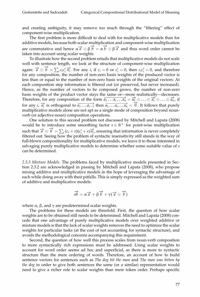
2.3.3 Mixture Models. The problems faced by multiplicative models presented in Sec-tion 2.3.2 are acknowledged in passing by Mitchell and Lapata (2008), who proposemixing additive and multiplicative models in the hope of leveraging the advantage ofeach while doing away with their pitfalls. This is simply expressed as the weighted sumof additive and multiplicative models:

−→ab = α−→a + β

−→b + γ(−→a �−→

b )

where α, β, and γ are predetermined scalar weights.The problems for these models are threefold. First, the question of how scalar

weights are to be obtained still needs to be determined. Mitchell and Lapata (2008) con-cede that one advantage of purely multiplicative models over weighted additive ormixture models is that the lack of scalar weights removes the need to optimize the scalarweights for particular tasks (at the cost of not accounting for syntactic structure), andavoids the methodological concerns accompanying this requirement.

Second, the question of how well this process scales from noun-verb compositionto more syntactically rich expressions must be addressed. Using scalar weights toaccount for word order seems ad hoc and superficial, as there is more to syntacticstructure than the mere ordering of words. Therefore, an account of how to buildsentence vectors for sentences such as The dog bit the man and The man was bitten bythe dog in order to give both sentences the same (or a similar) representation wouldneed to give a richer role to scalar weights than mere token order. Perhaps specific

77


weights could be given to particular syntactic classes (such as nouns) to introduce amore complex syntactic element into vector composition, but it is clear that this aloneis not a solution, as the weight for nouns dog and man would be the same, allowingfor the same commutative degeneracy observed in non-weighted additive models, inwhich

−−−−−−−−−−−−−−→the dog bit the man =

−−−−−−−−−−−−−−→the man bit the dog. Introducing a mixture of weighting

systems accounting for both word order and syntactic roles may be a solution, but it isnot only ad hoc but also arguably only partially reflects the syntactic structure of thesentence.

The third problem is that Mitchell and Lapata (2008) show that in practice, althoughmixture models perform better at verb disambiguation tasks than additive models andweighted additive models, they perform equivalently to purely multiplicative modelswith the added burden of requiring parametric optimization of the scalar weights.

Therefore, whereas mixture models aim to take the best of additive and multiplica-tive models while avoiding their problems, they are only partly successful in achievingthe latter goal, and demonstrably do little better in achieving the former.

2.3.4 Tensor-Based Models. From Sections 2.3.1–2.3.3 we observe that the need for incor-porating syntactic information into DSMs to achieve true compositionality is pressing,if only to develop a non-commutative composition operation that can take into accountword order without the need for adhoc weighting schemes, and hopefully richer syn-tactic information as well.

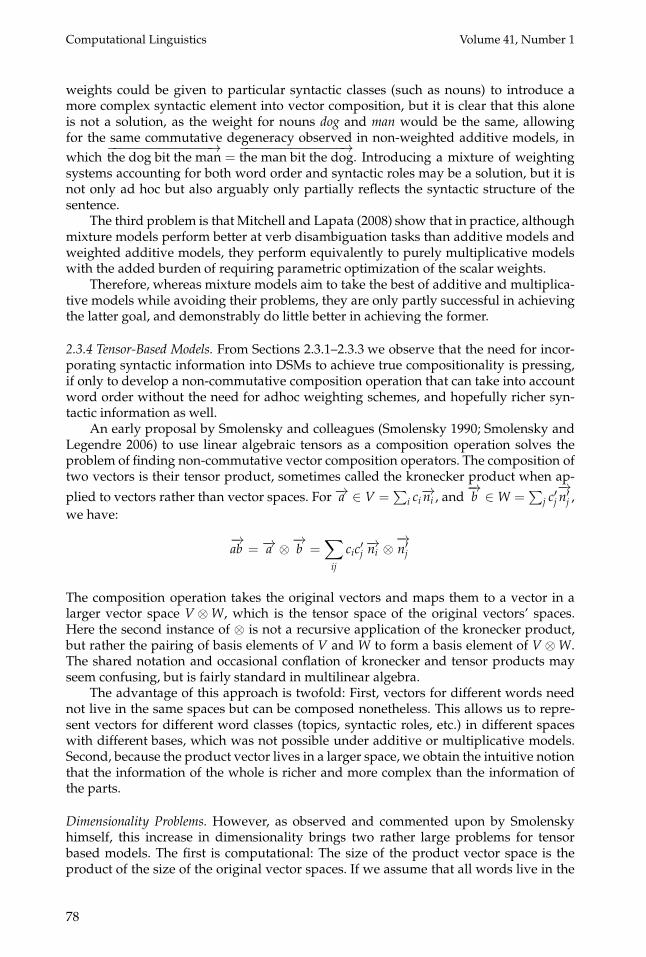
An early proposal by Smolensky and colleagues (Smolensky 1990; Smolensky andLegendre 2006) to use linear algebraic tensors as a composition operation solves theproblem of finding non-commutative vector composition operators. The composition oftwo vectors is their tensor product, sometimes called the kronecker product when ap-

plied to vectors rather than vector spaces. For −→a ∈ V =∑

i ci−→ni , and

−→b ∈ W =

∑j c′j

−→n′

j ,we have:

−→ab = −→a ⊗−→

b =∑

ij

cic′j−→ni ⊗

−→n′

j

The composition operation takes the original vectors and maps them to a vector in alarger vector space V ⊗ W, which is the tensor space of the original vectors’ spaces.Here the second instance of ⊗ is not a recursive application of the kronecker product,but rather the pairing of basis elements of V and W to form a basis element of V ⊗ W.The shared notation and occasional conflation of kronecker and tensor products mayseem confusing, but is fairly standard in multilinear algebra.

The advantage of this approach is twofold: First, vectors for different words neednot live in the same spaces but can be composed nonetheless. This allows us to repre-sent vectors for different word classes (topics, syntactic roles, etc.) in different spaceswith different bases, which was not possible under additive or multiplicative models.Second, because the product vector lives in a larger space, we obtain the intuitive notionthat the information of the whole is richer and more complex than the information ofthe parts.

Dimensionality Problems. However, as observed and commented upon by Smolenskyhimself, this increase in dimensionality brings two rather large problems for tensorbased models. The first is computational: The size of the product vector space is theproduct of the size of the original vector spaces. If we assume that all words live in the

78


same space N of dimensionality dim(N), then the dimensionality of an n-word sentencevector is dim(N)n. If we have as many basis vectors for our word semantic space asthere are lexemes in our vocabulary (e.g., approximately 170k in English2), then the sizeof our sentence vectors quickly reaches magnitudes for which vector comparison (oreven storage) are computationally intractable.3 Even if, as most DSM implementationsdo, we restrict the basis vectors of word semantic spaces to the k (e.g., k = 2,000) mostfrequent words in a corpus, the sentence vector size still grows exponentially withsentence length, and the implementation problems remain.

The second problem is mathematical: Sentences of different length live in differentspaces, and if we assign different vector spaces to different word types (e.g., syntacticclasses), then sentences of different syntactic structure live in different vector spaces,and hence cannot be compared directly using inner product or cosine measures, leavingus with no obvious mode of semantic comparison for sentence vectors. If any modelwishes to use tensor products in composition operations, it must find some way ofreducing the dimensionality of product vectors to some common vector space so thatthey may be directly compared.

One notable method by which these dimensionality problems can be solved ingeneral are the holographic reduced representations proposed by Plate (1991). Theproduct vector of two vectors is projected into a space of smaller dimensionality bycircular convolution to produce a trace vector. The circular correlation of the trace vectorand one of the original vectors produces a noisy version of the other original vector.The noisy vector can be used to recover the clean original vector by comparing it with apredefined set of candidates (e.g., the set of word vectors if our original vectors are wordmeanings). Traces can be summed to form new traces effectively containing several vec-tor pairs from which original vectors can be recovered. Using this encoding/decodingmechanism, the tensor product of sets of vectors can be encoded in a space of smallerdimensionality, and then recovered for computation without ever having to fully repre-sent or store the full tensor product, as discussed by Widdows (2008).

There are problems with this approach that make it unsuitable for our purposes,some of which are discussed in Mitchell and Lapata (2010). First, there is a limit tothe information that can be stored in traces, which is independent of the size of thevectors stored, but is a logarithmic function of their number. As we wish to be ableto store information for sentences of variable word length without having to directlyrepresent the tensored sentence vector, setting an upper bound to the number of vectorsthat can be composed in this manner limits the length of the sentences we can representcompositionally using this method.

Second, and perhaps more importantly, there are restrictions on the nature ofthe vectors that can be encoded in such a way: The vectors must be independentlydistributed such that the mean Euclidean length of each vector is 1. Such conditionsare unlikely to be met in word semantic vectors obtained from a corpus; and as thefailure to do so affects the system’s ability to recover clean vectors, holographic re-duced representations are not prima facie usable for compositional DSMs, although itis important to note that Widdows (2008) considers possible application areas wherethey may be of use, although once again these mostly involve noun-verb and adjective-noun compositionality rather than full blown sentence vector construction. We retain

2 Source: http://www.oxforddictionaries.com/page/howmanywords.3 At four bytes per integer, and one integer per basis vector weight, the vector for John loves Mary

would require roughly (170, 000 · 4)3 ≈ 280 petabytes of storage, which is over ten times the data Googleprocesses on a daily basis according to Dean and Ghemawat (2008).

79


from Plate (1991) the importance of finding methods by which to project the tensoredsentence vectors into a common space for direct comparison, as will be discussed furtherin Section 3.

Syntactic Expressivity. An additional problem of a more conceptual nature is that usingthe tensor product as a composition operation simply preserves word order. As wediscussed in Section 2.3.3, this is not enough on its own to model sentence meaning. Weneed to have some means by which to incorporate syntactic analysis into compositionoperations.

Early work on including syntactic sensitivity into DSMs by Grefenstette (1992)suggests using crude syntactic relations to determine the frame in which the distri-butions for word vectors are collected from the corpus, thereby embedding syntac-tic information into the word vectors. This idea was already present in the work ofSmolensky, who used sums of pairs of vector representations and their roles, obtainedby taking their tensor products, to obtain a vector representation for a compound. Theapplication of these ideas to DSMs was studied by Clark and Pulman (2007), whosuggest instantiating the roles to dependency relations and using the distributionalrepresentations of words as the vectors. For example, in the sentence Simon loves redwine, Simon is the subject of loves, wine is its object, and red is an adjective describingwine. Hence, from the dependency tree with loves as root node, its subject and object aschildren, and their adjectival descriptors (if any) as their children, we read the following

structure:−−−→loves ⊗−−→

subj ⊗−−−−→Simon ⊗−→

obj ⊗−−−→wine ⊗−→

adj ⊗−→red. Using the equality relation for

inner products of tensor products:

〈−→a ⊗−→b | −→c ⊗−→

d 〉 = 〈−→a | −→c 〉 × 〈−→b | −→d 〉

We can therefore express inner-products of sentence vectors efficiently without everhaving to actually represent the tensored sentence vector:

〈−−−−−−−−−−−−→Simon loves red wine | −−−−−−−−−−−−−−→Mary likes delicious rose〉

= 〈−−→loves ⊗−→subj ⊗−−→

Simon ⊗−→obj ⊗−−→

wine ⊗−→adj ⊗−→

red | −→likes ⊗−→

subj ⊗−−→Mary ⊗−→

obj ⊗−→rose ⊗−→

adj ⊗−−−−→delicious〉

= 〈−−→loves | −→likes〉× 〈−→subj | −→subj〉 × 〈−−→

Simon | −−→Mary〉 × 〈−→obj | −→obj〉 × 〈−−→wine | −→rose〉× 〈−→adj | −→adj 〉 × 〈−→red | −−−−→delicious〉

= 〈−−→loves | −→likes〉× 〈−−→

Simon | −−→Mary〉× 〈−−→wine | −→rose〉 × 〈−→red | −−−−→delicious〉

This example shows that this formalism allows for sentence comparison of sentenceswith identical dependency trees to be broken down to term-to-term comparison withoutthe need for the tensor products to ever be computed or stored, reducing computationto inner product calculations.

However, although matching terms with identical syntactic roles in the sentenceworks well in the given example, this model suffers from the same problems as theoriginal tensor-based compositionality of Smolensky (1990) in that, by the authors’own admission, sentences of different syntactic structure live in spaces of differentdimensionality and thus cannot be directly compared. Hence we cannot use this tomeasure the similarity between even small variations in sentence structure, such as thepair “Simon likes red wine” and “Simon likes wine.”

2.3.5 SVS Models. The idea of including syntactic relations to other lemmas in wordrepresentations discussed in Section 2.3.4 is applied differently in the structured vector

80


space model presented by Erk and Pado (2008). They propose to represent word mean-ings not as simple vectors, but as triplets:

w = (v, R, R−1)

where v is the word vector, constructed as in any other DSM, R and R−1 are selectionalpreferences, and take the form of R → D maps where R is the set of dependencyrelations, and D is the set of word vectors. Selectional preferences are used to encodethe lemmas that w is typically the parent of in the dependency trees of the corpus in thecase of R, and typically the child of in the case of R−1.

Composition takes the form of vector updates according to the following protocol.Let a = (va, Ra, R−1

a ) and b = (vb, Rb, R−1b ) be two words being composed, and let r be the

dependency relation linking a to b. The vector update procedure is as follows:

a′ = (va � R−1b (r), Ra − {r}, R−1

a )

b′ = (vb � Ra(r), Rb, R−1b − {r})

where a′, b′ are the updated word meanings, and � is whichever vector composition(addition, component-wise multiplication) we wish to use. The word vectors in thetriplets are effectively filtered by combination with the lemma which the word theyare being composed with expects to bear relation r to, and this relation between thecomposed words a and b is considered to be used and hence removed from the domainof the selectional preference functions used in composition.

This mechanism is therefore a more sophisticated version of the compositionaldisambiguation mechanism discussed by Mitchell and Lapata (2008) in that the com-bination of words filters the meaning of the original vectors that may be ambiguous(e.g., if we have one vector for bank); but contrary to Mitchell and Lapata (2008), theinformation of the original vectors is modified but essentially preserved, allowing forfurther combination with other terms, rather than directly producing a joint vector forthe composed words. The added fact that R and R−1 are partial functions associatedwith specific lemmas forces grammaticality during composition, since if a holds adependency relation r to b which it never expects to hold (for example a verb havingas its subject another verb, rather than the reverse), then Ra and R−1

b are undefined for rand the update fails. However, there are some problems with this approach if our goalis true compositionality.

First, this model does not allow some of the “repeated compositionality” we needbecause of the update of R and R−1. For example, we expect that an adjective composedwith a noun produces something like a noun in order to be further composed with a verbor even another adjective. However, here, because the relation adj would be removedfrom R−1

b for some noun b composed with an adjective a, this new representation b′would not have the properties of a noun in that it would no longer expect compositionwith an adjective, rendering representations of simple expressions like “the new redcar” impossible. Of course, we could remove the update of the selectional preferencefunctions from the compositional mechanism, but then we would lose this attractivefeature of grammaticality enforcement through the partial functionality of R and R−1.

Second, this model does little more than represent the implicit disambiguation thatis expected during composition, rather than actually provide a full blown compositionalmodel. The inability of this system to provide a novel mechanism by which to obtain

81


a joint vector for two composed lemmas—thereby building towards sentence vectors—entails that this system provides no means by which to obtain semantic representationsof larger syntactic structures that can be compared by inner product or cosine measureas is done with any other DSM. Of course, this model could be combined with thecompositional models presented in Sections 2.3.1–2.3.3 to produce sentence vectors, butwhereas some syntactic sensitivity would have been obtained, the word ordering andother problems of the aforementioned models would still remain, and little progresswould have been made towards true compositionality.

We retain from this attempt to introduce compositionality in DSMs that includinginformation obtained from syntactic dependency relations is important for proper dis-ambiguation, and that having some mechanism by which the grammaticality of theexpression being composed is a precondition for its composition is a desirable featurefor any compositional mechanism.

2.4 Matrix-Based Compositionality

The final class of approaches to vector composition we wish to discuss are threematrix-based models.

Generic Additive Model. The first is the Generic Additive Model of Zanzotto et al. (2010).This is a generalization of the weighted additive model presented in Section 2.3.1.In this model, rather than multiplying lexical vectors by fixed parameters α and βbefore adding them to form the representation of their combination, they are insteadthe arguments of matrix multiplication by square matrices A and B:

−→ab = A−→a + B

−→b

Here, A and B represent the added information provided by putting two words intorelation.

The numerical content of A and B is learned by linear regression over triplets(−→a ,

−→b ,−→c ) where −→a and

−→b are lexical semantic vectors, and −→c is the expected output

of the combination of −→a and−→b . This learning system thereby requires the provision of

labeled data for linear regression to be performed. Zanzotto et al. (2010) suggest severalsources for this labeled data, such as dictionary definitions and word etymologies.

This approach is richer than the weighted additive models because the matricesact as linear maps on the vectors they take as “arguments,” and thus can encode moresubtle syntactic or semantic relations. However, this model treats all word combinationsas the same operation—for example, treating the combination of an adjective with itsargument and a verb with its subject as the same sort of composition. Because of thediverse ways there are of training such supervised models, we leave it to those whowish to further develop this specific line of research to perform such evaluations.

Adjective Matrices. The second approach is the matrix-composition model of Baroni andZamparelli (2010), which they develop only for the case of adjective-noun composition,although their approach can seamlessly be used for any other predicate-argument com-position. Contrary to most of the earlier approaches proposed, which aim to combinetwo lexical vectors to form a lexical vector for their combination, Baroni and Zamparellisuggest giving different semantic representations to different types, or more specificallyto adjectives and nouns.

82


In this model, nouns are lexical vectors, as with other models. However, embracinga view of adjectives that is more in line with formal semantics than with distributionalsemantics, they model adjectives as linear maps taking lexical vectors as input and pro-ducing lexical vectors as output. Such linear maps can be encoded as square matrices,and applied to their arguments by matrix multiplication. Concretely, let Madjective be thematrix encoding the adjective’s linear map, and −−→noun be the lexical semantic vector fora noun; their combination is simply

−−−−−−−−−→adjective noun = Madjective ×−−→noun

Similarly to the Generic Additive Model, the matrix for each adjective is learnedby linear regression over a set of pairs (−−→noun,−→c ) where the vectors −−→noun are the lexicalsemantic vectors for the arguments of the adjective in a corpus, and −→c is the semanticvector corresponding to the expected output of the composition of the adjective withthat noun.

This may, at first blush, also appear to be a supervised training method for learn-ing adjective matrices from “labeled data,” seeing how the expected output vectorsare needed. However, Baroni and Zamparelli (2010) work around this constraint byautomatically producing the labeled data from the corpus by treating the adjective-noun compound as a single token, and learning its vector using the same distributionallearning methods they used to learn the vectors for nouns. This same approach can beextended to other unary relations without change and, using the general frameworkof the current article, an extension of it to binary predicates has been presented inGrefenstette et al. (2013), using multistep regression. For a direct comparison of theresults of this approach with some of the results of the current article, we refer thereader to Grefenstette et al. (2013).

Recursive Matrix-Vector Model. The third approach is the recently developed RecursiveMatrix-Vector Model (MV-RNN) of Socher et al. (2012), which claims the two matrix-based models described here as special cases. In MV-RNN, words are represented as apairing of a lexical semantic vector −→a with an operation matrix A. Within this model,given the parse of a sentence in the form of a binarized tree, the semantic representation(−→c , C) of each non-terminal node in the tree is produced by performing the followingtwo operations on its children (−→a , A) and (

−→b , B).

First, the vector component −→c is produced by applying the operation matrix of onechild to the vector of the other, and vice versa, and then projecting both of the productsback into the same vector space as the child vectors using a projection matrix W, whichmust also be learned:

−→c = W ×[

B ×−→aA ×−→

b

]

Second, the matrix C is calculated by projecting the pairing of matrices A and B backinto the same space, using a projection matrix WM, which must also be learned:

C = WM ×[

AB

]

83


The pairing (−→c , C) obtained through these operations forms the semantic representationof the phrase falling under the scope of the segment of the parse tree below that node.

This approach to compositionality yields good results in the experiments describedin Socher et al. (2012). It furthermore has appealing characteristics, such as treatingrelational words differently through their operation matrices, and allowing for recursivecomposition, as the output of each composition operation is of the same type of objectas its inputs. This approach is highly general and has excellent coverage of differentsyntactic types, while leaving much room for parametric optimization.

The principal mathematical difference with the compositional framework presentedsubsequently is that composition in MV-RNN is always a binary operation; for exam-ple, to compose a transitive verb with its subject and object one would first need tocompose it with its object, and then compose the output of that operation with thesubject. The framework we discuss in this article allows for the construction of largerrepresentations for relations of larger arities, permitting the simultaneous compositionof a verb with its subject and object. Whether or not this theoretical difference leads tosignificant differences in composition quality requires joint evaluation. Additionally,the description of MV-RNN models in Socher et al. (2012) specifies the need for asource of learning error during training, which is easy to measure in the case of labelprediction experiments such as sentiment prediction, but non-trivial in the case ofparaphrase detection where no objective label exists. A direct comparison to MV-RNNmethods within the context of experiments similar to those presented in this article hasbeen produced by Blacoe and Lapata (2012), showing that simple operations performon par with the earlier complex deep learning architectures produced by Socher andcolleagues; we leave direct comparisons to future work. Early work has shown that theaddition of a hidden layer with non-linearities to these simple models will improve theresults.

2.5 Some Other Approaches to Distributional Semantics

Domains and Functions. In recent work, Turney (2012) suggests modeling word repre-sentations not as a single semantic vector, but as a pair of vectors: one containing theinformation of the word relative to its domain (the other words that are ontologicallysimilar), and another containing information relating to its function. The former vectoris learned by looking at what nouns a word co-occurs with, and the latter is learnedby looking at what verb-based patterns the word occurs in. Similarity between sets ofwords is not determined by a single similarity function, but rather through a combi-nation of comparisons of the domain components of words’ representations with thefunction components of the words’ representations. Such combinations are designedon a task-specific basis. Although Turney’s work does not directly deal with vectorcomposition of the sort we explore in this article, Turney shows that similarity measurescan be designed for tasks similar to those presented here. The particular limitation ofhis approach, which Turney discusses, is that similarity measures must be specified foreach task, whereas most of the compositional models described herein produce repre-sentations that can be compared in a task-independent manner (e.g., through cosinesimilarity). Nonetheless, this approach is innovative, and will merit further attention infuture work in this area.

Language as Algebra. A theoretical model of meaning as context has been proposed inClarke (2009, 2012). In that model, the meaning of any string of words is a vector built

84


from the occurrence of the string in a corpus. This is the most natural extension ofdistributional models from words to strings of words: in that model, one builds vectorsfor strings of words in exactly the same way as one does for words. The main problem,however, is that of data sparsity for the occurrences of strings of words. Words doappear repeatedly in a document, but strings of words, especially for longer strings,rarely do so; for instance, it hardly happens that an exact same sentence appears morethan once in a document. To overcome this problem, the model is based on the hypo-thetical concept of an infinite corpus, an assumption that prevents it from being appliedto real-world corpora and experimented within natural language processing tasks. Onthe positive side, the model provides a theoretical study of the abstract properties ofa general bilinear associative composition operator; in particular, it is shown that thisoperator encompasses other composition operators, such as addition, multiplication,and even tensor product.

3. DisCoCat

In Section 2, we discussed lexical DSMs and the problems faced by attempts to providea vector composition operation that would allow us to form distributional sentence rep-resentations as a function of word meaning. In this section, we will present an existingformalism aimed at solving this compositionality problem, as well as the mathematicalbackground required to understand it and further extensions, building on the featuresand failures of previously discussed attempts at syntactically sensitive compositionality.

Clark, Coecke, and Sadrzadeh (2008) and Coecke, Sadrzadeh, and Clark (2010)propose adapting a category theoretic model, inspired by the categorical compositionalvector space model of quantum protocols (Abramsky and Coecke 2004), to the taskof compositionality of semantic vectors. Syntactic analysis in the form of pregroupgrammars—a categorial grammar—is given categorical semantics in order to be repre-sented as a compact closed category P (a concept explained subsequently), the objects ofwhich are syntactic types and the morphisms of which are the reductions forming thebasis of syntactic analysis. This syntactic category is then mapped onto the semanticcompact closed category FVect of finite dimensional vector spaces and linear maps.The mapping is done in the product category FVect × P via the following procedure.Each syntactic type is interpreted as a vector space in which semantic vectors for wordswith that particular syntactic type live; the reductions between the syntactic types areinterpreted as linear maps between the interpreted vector spaces of the syntactic types.

The key feature of category theory exploited here is its ability to relate in a canonicalway different mathematical formalisms that have similar structures, even if the originalformalisms belong in different branches of mathematics. In this context, it has enabledus to relate syntactic types and reductions to vector spaces and linear maps and obtaina mechanism by which syntactic analysis guides semantic composition operations.

This pairing of syntactic analysis and semantic composition ensures both thatgrammaticality restrictions are in place as in the model of Erk and Pado (2008) andsyntactically driven semantic composition in the form of inner-products provide the im-plicit disambiguation features of the compositional models of Erk and Pado (2008) andMitchell and Lapata (2008). The composition mechanism also involves the projection oftensored vectors into a common semantic space without the need for full representationof the tensored vectors in a manner similar to Plate (1991), without restriction to thenature of the vector spaces it can be applied to. This avoids the problems faced by othertensor-based composition mechanisms such as Smolensky (1990) and Clark and Pulman(2007).

85


The word vectors can be specified model-theoretically and the sentence space can bedefined over Boolean values to obtain grammatically driven truth-theoretic semanticsin the style of Montague (1974), as proposed by Clark, Coecke, and Sadrzadeh (2008).Some logical operators can be emulated in this setting, such as using swap matrices fornegation as shown by Coecke, Sadrzadeh, and Clark (2010). Alternatively, corpus-basedvariations on this formalism have been proposed by Grefenstette et al. (2011) to obtaina non-truth theoretic semantic model of sentence meaning for which logical operationshave yet to be defined.

Before explaining how this formalism works, in Section 3.3, we will introduce thenotions of pregroup grammars in Section 3.1, and the required basics of category theoryin Section 3.2.

3.1 Pregroup Grammars

Presented by Lambek (1999, 2008) as a successor to his syntactic calculus (Lambek 1958),pregroup grammars are a class of categorial type grammars with pregroup algebrasas semantics. Pregroups are particularly interesting within the context of this workbecause of their well-studied algebraic structure, which can trivially be mapped onto thestructure of the category of vector spaces, as will be discussed subsequently. Logicallyspeaking, a pregroup is a non-commutative form of Linear Logic (Girard 1987) in whichthe tensor and its dual par coincide; this logic is sometimes referred to as Bi-CompactLinear Logic (Lambek 1999). The formalism works alongside the general guidelines ofother categorial grammars, for instance, those of the combinatory categorial grammar(CCG) designed by Steedman (2001) and Steedman and Baldridge (2011). They consistof atomic grammatical types that combine to form compound types. A series of CCG-like application rules allow for type-reductions, forming the basis of syntactic analysis.As our first step, we show how this syntactic analysis formalism works by presentingan introduction to pregroup algebras.

Pregroups. A pregroup is an algebraic structure of the form (P,≤, ·, 1, (−)l, (−)r). Itselements are defined as follows:

� P is a set {a, b, c, . . .}.� The relation ≤ is a partial ordering on P.� The binary operation · is an associative, non-commutative monoid

multiplication with the type − · − : P × P → P, such that if a, b ∈ P thena · b ∈ P. In other words, P is closed under this operation.

� 1 ∈ P is the unit, satisfying a · 1 = a = 1 · a for all a ∈ P.� (−)l and (−)r are maps with types (−)l : P → P and (−)r : P → P such that

for any a ∈ P, we have that al, ar ∈ P. The images of these maps arereferred to as the left and the right adjoints. These are unique and satisfythe following conditions:

– Reversal: if a ≤ b then bl ≤ al (and similarly for ar, br).– Ordering: a · ar ≤ 1 ≤ ar · a and al · a ≤ 1 ≤ a · al.– Cancellation: alr = a = arl.– Self-adjointness of identity: 1r = 1 = 1l.– Self-adjointness of multiplication: (a · b)r = br · ar.

86


As a notational simplification we write ab for a · b, and if abcd ≤ cd we write abcd →cd and call this a reduction, omitting the identity wherever it might appear. Monoidmultiplication is associative, so parentheses may be added or removed for notationalclarity without changing the meaning of the expression as long as they are not directlyunder the scope of an adjoint operator.

An example reduction in pregroup might be:

aarbclc → bclc → b

We note here that the reduction order is not always unique, as we could have reduced asfollows: aarbclc → aarb → b. As a further notational simplification, if there exists a chainof reductions a → . . . → b we may simply write a → b (in virtue of the transitivity ofpartial ordering relations). Hence in our given example, we can express both reductionpaths as aarbclc → b.

Pregroups and Syntactic Analysis. Pregroups are used for grammatical analysis by freelygenerating the set P of a pregroup from the basic syntactic types n, s, . . . , where heren stands for the type of both a noun and a noun phrase and s for that of a sentence.The conflation of nouns and noun phrases suggested here is done to keep the workdiscussed in this article as simple as possible, but we could of course model them asdifferent types in a more sophisticated version of this pregroup grammar. As in anycategorial grammar, words of the lexicon are assigned one or more possible types(corresponding to different syntactic roles) in a predefined type dictionary, and thegrammaticality of a sentence is verified by demonstrating the existence of a reductionfrom the combination of the types of words within the sentence to the sentence type s.

For example, having assigned to noun phrases the type n and to sentences the type s,the transitive verbs will have the compound type nrsnl. We can read from the type ofa transitive verb that it is the type of a word which “expects” a noun phrase on its leftand a noun phrase on its right, in order to produce a sentence. A sample reduction ofJohn loves cake with John and cake being noun phrases of type n and loves being a verb oftype nrsnl is as follows:

n(nrsnl)n → s

We see that the transitive verb has combined with the subject and object to reduce to asentence. Because the combination of the types of the words in the string John loves cakereduces to s, we say that this string of words is a grammatical sentence. As for moreexamples, we recall that intransitive verbs can be given the type nrs such that John sleepswould be analyzed in terms of the reduction n(nrs) → s. Adjectives can be given thetype nnl such that red round rubber ball would be analyzed by (nnl)(nnl)(nnl)n → n. Andso on and so forth for other syntactic classes.

Lambek (2008) presents the details of a slightly more complex pregroup grammarwith a richer set of types than presented here. This grammar is hand-constructed anditeratively extended by expanding the type assignments as more sophisticated gram-matical constructions are discussed. No general mechanism is proposed to cover allsuch types of assignments for larger fragments (e.g., as seen in empirical data). Pregroupgrammars have been proven to be learnable by Bechet, Foret, and Tellier (2007), whoalso discuss the difficulty of this task and the nontractability of the procedure. Becauseof these constraints and lack of a workable pregroup parser, the pregroup grammars

87


we will use in our categorical formalism are derived from CCG types, as we explain inthe following.

Pregroup Grammars and Other Categorial Grammars. Pregroup grammars, in contrast withother categorial grammars such as CCG, do not yet have a large set of tools for parsingavailable. If quick implementation of the formalism described later in this paper isrequired, it would be useful to be able to leverage the mature state of parsing toolsavailable for other categorial grammars, such as the Clark and Curran (2007) statisticalCCG parser, as well as Hockenmaier’s CCG lexicon and treebank (Hockenmaier 2003;Hockenmaier and Steedman 2007). In other words, is there any way we can translate atleast some subset of CCG types into pregroup types?

There are some theoretical obstacles to consider first: Pregroup grammars and CCGare not equivalent. Buszkowski (2001) shows pregroup grammars to be equivalent tocontext-free grammars, whereas Joshi, Vijay-Shanker, and Weir (1989) show CCG to beweakly equivalent to more expressive mildly context-sensitive grammars. However, ifour goal is to exploit the CCG used in Clark and Curran’s parser, or Hockenmaier’slexicon and treebank, we may be in luck: Fowler and Penn (2010) prove that someCCGs, such as those used in the aforementioned tools, are strongly context-free and thusexpressively equivalent to pregroup grammars. In order to be able to apply the parsingtools for CCGs to our setting, we use a translation mechanism from CCG types to pre-group types based on the Lambek-calculus-to-pregroup-grammar translation originallypresented in Lambek (1999). In this mechanism, each atomic CCG type X is assigned aunique pregroup type x; for any X/Y in CCG we have xyl in the pregroup grammar; andfor any X\Y in CCG we have yrx in pregroup grammar. Therefore, by assigning NP to nand S to s we could, for example, translate the CCG transitive verb type (S\NP)/NP intothe pregroup type nrsnl, which corresponds to the pregroup type we used for transitiveverbs in Section 3.1. Wherever type replacement (e.g., N → NP) is allowed in CCG weset an ordering relation in the pregroup grammar (e.g., n ≤ n, where n is the pregrouptype associated with N). Because forward and backward slash “operators” in CCG arenot associative whereas monoid multiplication in pregroups is, it is evident that someinformation is lost during the translation process. But because the translation we needis one-way, we may ignore this problem and use CCG parsing tools to obtain pregroupparses. Another concern lies with CCG’s crossed composition and substitution rules.The translations of these rules do not in general hold in a pregroup; this is not a surpriseas pregroups are a simplification of the Lambek Calculus and these rules did not holdin the Lambek Calculus either, as shown in Moortgat (1997), for example. However, forthe phenomena modeled in this paper, the CCG rules without the backward cross ruleswill suffice. In general for the case of English, one can avoid the use of these rules byoverloading the lexicon and using additional categories. To deal with languages thathave cross dependancies, such as Dutch, various solutions have been suggested (e.g.,see Genkin, Francez, and Kaminski 2010; Preller 2010).

3.2 Categories

Category theory is a branch of pure mathematics that allows for a general and uniformformulation of various different mathematical formalisms in terms of their main struc-tural properties using a few abstract concepts such as objects, arrows, and combinationsand compositions of these. This uniform conceptual language allows for derivationof new properties of existing formalisms and for relating these to properties of otherformalisms, if they bear similar categorical representation. In this function, it has been

88


at the center of recent work in unifying two orthogonal models of meaning, a qualitativecategorial grammar model and a quantitative distributional model (Clark, Coecke, andSadrzadeh 2008; Coecke, Sadrzadeh, and Clark 2010). Moreover, the unifying categori-cal structures at work here were inspired by the ones used in the foundations of physicsand the modeling of quantum information flow, as presented in Abramsky and Coecke(2004), where they relate the logical structure of quantum protocols to their state-basedvector spaces data. The connection between the mathematics used for this branch ofphysics and those potentially useful for linguistic modeling has also been noted byseveral sources, such as Widdows (2005), Lambek (2010), and Van Rijsbergen (2004).

In this section, we will briefly examine the basics of category theory, monoidalcategories, and compact closed categories. The focus will be on defining enough ba-sic concepts to proceed rather than provide a full-blown tutorial on category theoryand the modeling of information flow, as several excellent sources already cover bothaspects (e.g., Mac Lane 1998; Walters 1991; Coecke and Paquette 2011). A categories-in-a-nutshell crash course is also provided in Clark, Coecke, and Sadrzadeh (2008) andCoecke, Sadrzadeh, and Clark (2010).

The Basics of Category Theory. A basic category C is defined in terms of the followingelements:

� A collection of objects ob(C).� A collection of morphisms hom(C).� A morphism composition operation ◦.

Each morphism f has a domain dom( f ) ∈ ob(C) and a codomain codom( f ) ∈ ob(C).For dom( f ) = A and codom( f ) = B we abbreviate these definitions as f : A → B. Despitethe notational similarity to function definitions (and sets and functions being an ex-ample of a category), it is important to state that nothing else is presupposed aboutmorphisms, and we should not treat them a priori as functions.

The following axioms hold in every category C :

� For any f : A → B and g : B → C there exists h : A → C and h = g ◦ f .� For any f : A → B, g : B → C and h : C → D, ◦ satisfies

(h ◦ g) ◦ f = h ◦ (g ◦ f ).� For every A ∈ ob(C) there is an identity morphism idA : A → A such

that for any f : A → B, f ◦ idA = f = idB ◦ f .

We can model various mathematical formalisms using these basic concepts, andverify that these axioms hold for them. For example, category Set with sets as objects andfunctions as morphisms, or category Rel with sets as objects and relations as morphisms,category Pos with posets as objects and order-preserving maps as morphisms, andcategory Group with groups as objects and group homomorphisms as morphisms, toname a few.

The product C × D of two categories C and D is a category with pairs (A, B) asobjects, where A ∈ ob(C) and B ∈ ob(D). There exists a morphism (f, g) : (A, B) → (C, D)in C × D if and only if there exists f : A → C ∈ hom(C) and g : B → D ∈ hom(D). Productcategories allow us to relate objects and morphisms of one mathematical formalism tothose in another, in this example those of C to D.

89


Compact Closed Categories. A monoidal category C is a basic category to which we add amonoidal tensor ⊗ such that:

� For all A, B ∈ ob(C) there is an object A ⊗ B ∈ ob(C).� For all A, B, C ∈ ob(C), we have (A ⊗ B) ⊗ C = A ⊗ (B ⊗ C).� There exists some I ∈ ob(C) such that for any A ∈ ob(C), we have

I ⊗ A = A = A ⊗ I.� For f : A → C and g : B → D in hom(C) there is f ⊗ g : A ⊗ B → C ⊗ D in

hom(C).� For f1 : A → C, f2 : B → D, g1 : C → E and g2 : D → F the following

equality holds:

(g1 ⊗ g2) ◦ ( f1 ⊗ f2) = (g1 ◦ f1) ⊗ (g2 ◦ f2)

The product category of two monoidal categories has a monodial tensor, defined point-wisely by (a, A) ⊗ (b, B) := (a ⊗ b, A ⊗ B).

A compact closed category C is a monoidal category with the following additionalaxioms:

� Each object A ∈ ob(C) has left and right “adjoint” objects Al and Ar inob(C).

� There exist four structural morphisms for each object A ∈ ob(C):

– ηlA : I → A ⊗ Al.

– ηrA : I → Ar ⊗ A.

– εlA : Al ⊗ A → I.

– εrA : A ⊗ Ar → I.

� The previous structural morphisms satisfy the following equalities:

– (1A ⊗ εlA) ◦ (ηl

A ⊗ 1A) = 1A.– (εr

A ⊗ 1A) ◦ (1A ⊗ ηrA) = 1A.

– (1Ar ⊗ εrA) ◦ (ηr ⊗ 1Ar ) = 1Ar .

– (εlA ⊗ 1Al ) ◦ (1Al ⊗ ηl

A) = 1Al .

Compact closed categories come equipped with complete graphical calculi, sur-veyed in Selinger (2010). These calculi visualize and simplify the axiomatic reasoningwithin the category to a great extent. In particular, Clark, Coecke, and Sadrzadeh(2008) and Coecke, Sadrzadeh, and Clark (2010) show how they depict the pregroupgrammatical reductions and visualize the flow of information in composing meaningsof single words and forming meanings for sentences. Although useful at an abstractlevel, these calculi do not play the same simplifying role when it comes to the concreteand empirical computations; therefore we will not discuss them in this article.

A very relevant example of a compact closed category is a pregroup algebra P.Elements of a pregroup are objects of the category, the partial ordering relation providesthe morphisms, 1 is I, and monoidal multiplication is the monoidal tensor.

Another very relevant example is the category FVect of finite dimensional Hilbertspaces and linear maps over R—that is, vector spaces over R with orthogonal basesof finite dimension, and an inner product operation 〈− | −〉 : A × A → R for everyvector space A. The objects of FVect are vector spaces, and the morphisms are linear

90


maps between vector spaces. The unit object is R and the monoidal tensor is the linearalgebraic tensor product. FVect is degenerate in its adjoints, in that for any vector spaceA, we have Al = Ar = A∗, where A∗ is the dual space of A. Moreover, by fixing a basis weobtain that A∗ ∼= A. As such, we can effectively do away with adjoints in this category,and “collapse” εl, εr, ηl, and ηr maps into “adjoint-free” ε and η maps. In this category,the εmaps are inner product operations, εA : A ⊗ A → R, and the η maps η : R → A ⊗ Agenerate maximally entangled states, also referred to as Bell-states.

3.3 A Categorical Passage from Grammar to Semantics

In Section 3.2 we showed how a pregroup algebra and vector spaces can be modeledas compact closed categories and how product categories allow us to relate the objectsand morphisms of one category to those of another. In this section, we will present howClark, Coecke, and Sadrzadeh (2008) and Coecke, Sadrzadeh, and Clark (2010) suggestbuilding on this by using categories to relate semantic composition to syntactic analysisin order to achieve syntax-sensitive composition in DSMs.

3.3.1 Syntax Guides Semantics. The product category FVect × P has as object pairs (A, a),where A is a vector space and a is a pregroup grammatical type, and as morphism pairs( f,≤) where f is a linear map and ≤ a pregroup ordering relation. By the definition ofproduct categories, for any two vector space-type pairs (A, a) and (B, b), there existsa morphism (A, a) → (B, b) only if there is both a linear map from A into B and apartial ordering a → b. If we view these pairings as the association of syntactic typeswith vector spaces containing semantic vectors for words of that type, this restrictioneffectively states that a linear map from A to B is only “permitted” in the productcategory if a reduces to b.

Both P and FVect being compact closed, it is simple to show that FVect × P is as well,by considering the pairs of unit objects and structural morphisms from the separatecategories: I is now (R, 1), and the structural morphisms are (εA, εl

a), (εA, εra), (ηA,ηl

a),and (ηA,ηr

a). We are particularly interested in the ε maps, which are defined as follows(from the definition of product categories):

(εA, εlA) : (A ⊗ A, ala) → (R, 1) (εA, εr

A) : (A ⊗ A, aar) → (R, 1)

This states that whenever there is a reduction step in the grammatical analysis of asentence, there is a composition operation in the form of an inner product on thesemantic front. Hence, if nouns of type n live in some noun space N and transitiveverbs of type nlsnr live in some space N ⊗ S ⊗ N, then there must be some structuralmorphism of the form:

(εN ⊗ 1S ⊗ εN, εrn1sε

ln) : (N ⊗ (N ⊗ S ⊗ N) ⊗ N, n(nrsnl)n) → (S, s)

We can read from this morphism the functions required to compose a sentence with anoun, a transitive verb, and an object to obtain a vector living in some sentence space S,namely, (εN ⊗ 1S ⊗ εN ).

The form of a syntactic type is therefore what dictates the structure of the semanticspace associated with it. The structural morphisms of the product category guaranteethat for every syntactic reduction there is a semantic composition morphism providedby the product category: syntactic analysis guides semantic composition.

91


3.3.2 Example. To give an example, we give syntactic type n to nouns, and nrs to intran-sitive verbs. The grammatical reduction for kittens sleep, namely, nnrs → s, correspondsto the morphism εr

n ⊗ 1s in P. The syntactic types dictate that the noun−−−−→kittens lives

in some vector space N, and the intransitive verb−−−→sleep in N ⊗ S. The reduction mor-

phism gives us the composition morphism (εN ⊗ 1S), which we can apply to−−−−→kittens

⊗−−−→sleep.

Because we can express any vector as the weighted sum of its basis vectors, letus expand

−−−−→kittens =

∑i ckittens

i−→ni and

−−−→sleep =

∑ij csleep

ij−→ni ⊗−→sj ; then we can express the

composition as follows:

−−−−−−−−→kittens sleep = (εN ⊗ 1S)(

−−−−→kittens ⊗−−−→

sleep)

= (εN ⊗ 1S)

⎛⎝∑

i

ckittensi

−→ni ⊗∑

jk

csleepjk

−→nj ⊗−→sk

⎞⎠

= (εN ⊗ 1S)

⎛⎝∑

ijk

ckittensi csleep

jk−→ni ⊗−→nj ⊗−→sk

⎞⎠

=∑

ijk

ckittensi csleep

jk 〈−→ni | −→nj 〉−→sk

=∑

ik

ckittensi csleep

ik−→sk

In these equations, we have expressed the vectors in their explicit form, we haveconsolidated the sums by virtue of distributivity of linear algebraic tensor product overaddition, we have applied the tensored linear maps to the vector components (as theweights are scalars), and finally, we have simplified the indices since 〈−→ni | −→nj 〉 = 1 if−→ni =

−→nj and 0 otherwise. As a result of these, we have obtained a vector that lives insentence space S.

Transitive sentences can be dealt with in a similar fashion:

−−−−−−−−−−−−−→kittens chase mice

= (εN ⊗ 1S ⊗ εN)(−−−−→kittens ⊗−−−→

chase ⊗−−→mice)

= (εN ⊗ 1S ⊗ εN)

⎛⎝∑

i

ckittensi

−→ni ⊗⎛⎝∑

jkl

cchasejkl

−→nj ⊗−→sk ⊗−→nl

⎞⎠⊗

∑m

cmicem

−→nm

⎞⎠

= (εN ⊗ 1S ⊗ εN)

⎛⎝∑

ijklm

ckittensi cchase

jkl cmicem

−→ni ⊗−→nj ⊗−→sk ⊗−→nl ⊗−→nm

⎞⎠

=∑ijklm

ckittensi cchase

jkl cmicem 〈−→ni | −→nj 〉−→sk 〈−→nl | −→nm〉

=∑ikm

ckittensi cchase

ikm cmicem

−→sk

92


In both cases, it is important to note that the tensor product passed as argumentto the composition morphism, namely,

−−−−→kittens ⊗−−−→

sleep in the intransitive case and−−−−→kittens ⊗−−−→

chase ⊗−−→mice in the transitive case, never needs to be computed. We can

treat the tensor products here as commas separating function arguments, therebyavoiding the dimensionality problems presented by earlier tensor-based approaches tocompositionality.

3.4 This Article and the DisCoCat Literature

As elaborated on in Section 2.3.4, the first general setting for pairing meaning vec-tors with syntactic types was proposed in Clark and Pulman (2007). The setting of aDisCoCat generalized this by making the meaning derivation process rely on a syntactictype system, hence overcoming its central problem whereby the vector representationsof strings of words with different grammatical structure lived in different spaces. Apreliminary version of a DisCoCat was developed in Clark, Coecke, and Sadrzadeh(2008), a full version was elaborated on in Coecke, Sadrzadeh, and Clark (2010), where,based on the developments of Preller and Sadrzadeh (2010), it was also exemplifiedhow the vector space model may be instantiated in a truth theoretic setting wheremeanings of words were sets of their denotations and meanings of sentences were theirtruth values. A nontechnical description of this theoretical setting was presented inClark (2013), where a plausibility truth-theoretic model for sentence spaces was workedout and exemplified. The work of Grefenstette et al. (2011) focused on a tangentialbranch and developed a toy example where neither words nor sentence spaces wereBoolean. The applicability of the theoretical setting to a real empirical natural languageprocessing task and data from a large scale corpus was demonstrated in Grefenstetteand Sadrzadeh (2011a, 2011b). There, we presented a general algorithm to build vectorrepresentations for words with simple and complex types and the sentences containingthem; then applied the algorithm to a disambiguation task performed on the BritishNational Corpus (BNC). We also investigated the vector representation of transitiveverbs and showed how a number of single operations may optimize the performance.We discuss these developments in detail in the following sections.

4. Concrete Semantic Spaces

In Section 3.3 we presented a categorical formalism that relates syntactic analysissteps to semantic composition operations. The structure of our syntactic representationdictates the structure of our semantic spaces, but in exchange, we are provided withcomposition functions by the syntactic analysis, rather than having to stipulate themad hoc. Whereas the approaches to compositional DSMs presented in Section 2 eitherfailed to take syntax into account during composition, or did so at the cost of not beingable to compare sentences of different structure in a common space, this categoricalapproach projects all sentences into a common sentence space where they can be directlycompared. However, this alone does not give us a compositional DSM.

As we have seen in the previous examples, the structure of semantic spaces varieswith syntactic types. We therefore cannot construct vectors for different syntactic typesin the same way, as they live in spaces of different structure and dimensionality. Further-more, nothing has yet been said about the structure of the sentence space S into whichexpressions reducing to type s are projected. If we wish to have a compositional DSM

93


that leverages all the benefits of lexical DSMs and ports them to sentence-level distribu-tional representations, we must specify a new sort of vector construction procedure.

In the original formulation of this formalism by Clark, Coecke, and Sadrzadeh(2008) and Coecke, Sadrzadeh, and Clark (2010), examples of how such a compositionalDSM could be used for logical evaluation are presented, where S is defined as a Booleanspace with True and False as basis vectors. However, the word vectors used are hand-written and specified model-theoretically, as the authors leave it for future research todetermine how such vectors might be obtained from a corpus. In this section, we willdiscuss a new way of constructing vectors for compositional DSMs, and of definingsentence space S, in order to reconcile this powerful categorical formalism with theapplicability and flexibility of standard distributional models.

4.1 Defining Sentence Space

Assume the following sentences are all true:

1. The dogs chased the cats.

2. The dogs annoyed the cats.

3. The puppies followed the kittens.

4. The train left the station.

5. The president followed his agenda.

If asked which sentences have similar meaning, we would most likely point to thepair (1) and (3), and perhaps to a lesser degree (1) and (2), and (2) and (3). Sentences (4)and (5) obviously speak of a different state of the world as the other sentences.

If we compare these by truth value, we obviously have no means of making suchdistinctions. If we compare these by lexical similarity, (1) and (2) seem to be a closermatch than (1) and (3). If we are classifying these sentences by some higher orderrelation such as “topic,” (5) might end up closer to (3) than (1). What, then, might causeus to pair (1) and (3)?

Intuitively, this similarity seems to be because the subjects and objects brought intorelation by similar verbs are themselves similar. Abstracting away from tokens to somenotion of property, we might say that both (1) and (3) express the fact that somethingfurry and feline and furtive is being pursued by something aggressive (or playful)and canine. Playing along with the idea that lexical distributional semantics presentconcepts (word meanings) as “messy bundles of properties,” it seems only natural tohave the way these properties are acted upon, qualified, and related as the basis forsentence-level distributional representations. In this respect, we here suggest that thesentence space S, instead of qualifying the truth value of a sentence, should expresshow the properties of the semantic objects within are qualified or brought into relationby verbs, adjectives, and other predicates and relations.

More specifically, we examine two suggestions for defining the sentence space,namely, SI

∼= N for sentences with intransitive verbs and ST∼= N ⊗ N for sentences

with transitive verbs. These definitions mean that the sentence space’s dimensions arecommensurate with either those of N, or those of N ⊗ N. These are by no means theonly options, but as we will discuss here, they offer practical benefits.

In the case of SI, the basis elements are labeled with unique basis elements of N,hence, −→s1 = −→n1 , −→s2 = −→n2, and so on. In the case of ST, the basis elements are labeled with

94


unique ordered pairs of elements from N, for example, −→s1 =−−−−→(n1, n1), −→s2 =

−−−−→(n2, n1), −→s3 =−−−−→

(n1, n2), and so on, following the same matrix flattening structure used in the proof ofthe equal cardinality of N and Q. Because of the isomorphism between ST and N ⊗ N, wewill use the notations

−−−−→(ni, nj) and −→ni ⊗−→nj interchangeably, as both constitute appropriate

ways of representing the basis elements of such a space. To propagate this distinctionon the syntactic level, we define types sI and sT for intransitive and transitive sentences,respectively.

In creating this distinction, we lost one of the most appealing features of the frame-work of Coecke, Sadrzadeh, and Clark (2010), namely, the result that all sentence vectorslive in the same sentence space. A mathematical solution to this two-space problem wassuggested in Grefenstette et al. (2011), and a variant of the models presented in thisarticle permitting the non-problematic projection into a single sentence space (S ∼= N)has been presented by Grefenstette et al. (2013). Keeping this separation allows us todeal with both the transitive and intransitive cases in a simpler manner, and becausethe experiments in this article only compare intransitive sentences with intransitivesentences, and transitive sentences with transitive sentences, we will not address theissue of unification here.

4.2 Noun-Oriented Types

While Lambek’s pregroup types presented in Lambek (2008) include a rich array ofbasic types and hand-designed compound types in order to capture specific grammaticproperties, for the sake of simplicity we will use a simpler set of grammatical typesfor experimental purposes, similar to some common types found in the CCG-bank(Steedman 2001).

We assign a basic pregroup type n for all nouns, with an associated vector space Nfor their semantic representations. Furthermore, we will treat noun-phrases as nouns,assigning to them the same pregroup type and semantic space.

CCG treats intransitive verbs as functions NP\S that consume a noun phrase andreturn a sentence, and transitive verbs as functions (NP\S)/NP that consume a nounphrase and return an intransitive verb function, which in turn consumes a noun phraseand returns a sentence. Using our distinction between intransitive sentences, we giveintransitive verbs the type nrsI associated with the semantic space N ⊗ SI, and transitiveverbs the type nrsTnl associated with the semantic space N ⊗ ST ⊗ N.

Adjectives, in CCG, are treated as functions NP/NP, consuming a noun phrase andreturning a noun phrase; and hence we give them the type nnl and associated semanticspace N ⊗ N.

With the provision of a learning procedure for vectors in these semantic spaces, wecan use these types to construct sentence vector representations for simple intransitiveverb–based and transitive verb–based sentences, with and without adjectives appliedto subjects and objects.

4.3 Learning Procedures

To begin, we construct the semantic space N for all nouns in our lexicon (typically lim-ited by the words available in the corpus used). Any distributional semantic model canbe used for this stage, such as those presented in Curran (2004), or the lexical semanticmodels used by Mitchell and Lapata (2008). It seems reasonable to assume that higherquality lexical semantic vectors—as measured by metrics such as the WordSim353 test

95


of Finkelstein et al. (2001)—will produce better relational vectors from the proceduredesigned subsequently. We will not test the hypothesis here, but note that it is anunderlying assumption in most of the current literature on the subject (Erk and Pado2008; Mitchell and Lapata 2008; Baroni and Zamparelli 2010).

Building upon the foundation of the thus constructed noun vectors, we constructsemantic representations for relational words. In pregroup grammars (or other com-binatorial grammars such as CCG), we can view such words as functions, taking asarguments those types present as adjoints in the compound pregroup type, and return-ing a syntactic object whose type is that of the corresponding reduction. For example,an adjective nnl takes a noun or noun phrase n and returns a noun phrase n from thereduction (nnl)n → n. It can also compose with another adjective to return an adjective(nnl)(nnl) → nnl. We wish for our semantic representations to be viewed in the sameway, such that the composition of an adjective with a noun (1N ⊗ εN)((N ⊗ N) ⊗ N) canbe viewed as the application of a function f : N → N to its argument of type N.

To learn the representation of such functions, we assume that their meaning canbe characterized by the properties that their arguments hold in the corpus, rather thanjust by their context as is the case in lexical distributional semantic models. To givean example, rather than learning what the adjective angry means by observing thatit co-occurs with words such as fighting, aggressive, or mean, we learn its meaning byobserving that it typically takes as argument words that have the property of being(i.e., co-occur with words such as) fighting, aggressive, and mean. Whereas in the lexicalsemantic case, such associations might only rarely occur in the corpus, in this indirectmethod we learn what properties the adjective relates to even if they do not co-occurwith it directly.

In turn, through composition with its argument, we expect the function for suchan adjective to strengthen the properties that characterize it in the object it takes asargument. If, indeed, angry is characterized by arguments that have high basis weightsfor basis elements corresponding to the concepts (or context words) fighting, aggressive,and mean, and relatively low counts for semantically different concepts such as passive,peaceful, and loves, then when we apply angry to dog the vector for the compoundangry dog should contain some of the information found in the vector for dog. But thisvector should also have higher values for the basis weights of fighting, aggressive, andmean, and correspondingly lower values for the basis weights of passive, peaceful, andloves.

To turn this idea into a concrete algorithm for constructing the semantic repre-sentation for relations of any arity, as first presented in Grefenstette et al. (2011), weexamine how we would deal with this for binary relations such as transitive verbs. Ifa transitive verb of semantic type N ⊗ ST ⊗ N is viewed as a function f : N × N → STthat expresses the extent to which the properties of subject and object are brought intorelation by the verb, we learn the meaning of the verb by looking at what properties arebrought into relation by its arguments in a corpus. Recall that the vector for a verb v,−→v ∈ N ⊗ ST ⊗ N, can be expressed as the weighted sum of its basis elements:

−→v =∑

ijk

cvijk−→ni ⊗−→sj ⊗−→nk

We take the set of vectors for the subject and object of v in the corpus to be argv =

{(−−−−→SUBJl,

−−−→OBJl )}l. We wish to calculate the basis weightings {cv

ijk}ijk for v. Exploiting ourearlier definition of the basis {sj}j of ST, which states that for any value of i and k there

96


is some value of j such that sj = (ni, nk), we define Δijk = 1 if indeed sj = (ni, nk) and 0otherwise. Using all of this, we define the calculation of each basis weight cv

ijk as:

cvijk =

∑l

ΔijkcSUBJli cOBJl

k

This allows for a full formulation of −→v as follows:

−→v =∑

l

∑ijk

ΔijkcSUBJli cOBJl

k−→ni ⊗−→sj ⊗−→nk

The nested sums here may seem computationally inefficient, seeing how thiswould involve computing size(argv) × dim(N)2 × dim(S) = size(argv) × dim(N)4 prod-ucts. However, using the decomposition of basis elements of S into pairs of basiselements of N (effectively basis elements of N ⊗ N), we can remove the Δijk term andignore all values of j where sj �= (ni, nk), because the basis weight for this combinationof indices would be 0. Hence we simplify:

−→v =∑

l

∑ik

cSUBJli cOBJl

k−→ni ⊗

−−−−→(ni, nk) ⊗−→nk

This representation is still bloated: We perform fewer calculations, but still obtain avector in which all the basis weights where sj �= (ni, nk) are 0, hence where only dim(N)2

of the dim(N)4 values are non-zero. In short, the vector weights for −→v are, under thislearning algorithm, entirely characterized by the values of a dim(N) by dim(N) matrix,the entries of which are products cSUBJl

i cOBJlk where i and k have become row and column

indices.Using this and our definition of ST as a space isomorphic to N ⊗ N, we can formu-

late a compact expression of −→v as follows. Let the kronecker product of two vectors−→u ,−→w ∈ N, written −→u ⊗−→w ∈ N ⊗ N, be as follows:

−→u ⊗−→w =∑

ij

cui cw

j−→ni ⊗−→nj

Equipped with this definition, we can formulate the compact form of −→v :

−→v =∑

l

∑ik

cSUBJli cOBJl

k−→ni ⊗−→nk

=∑

l

−−−→SUBJl ⊗

−−→OBJl

In short, we are only required to iterate through the corpus once, taking for eachinstance of a transitive verb v the kronecker product of its subject and object, andsumming these across all instances of v. It is simple to see that no information wasdiscarded relative to the previous definition of −→v : The dimensionality reduction by afactor of dim(N)2 simply discards all basis elements for which the basis weight was 0 bydefault.

97


This raises a small problem though: This compact representation can no longer beused in the compositional mechanism presented in Section 3.3, as the dimensions of−→v no longer match those that it is required to have according to its syntactic type.However, a solution can be devised if we return to the sample calculation shown inSection 3.3.2 of the composition of a transitive verb with its arguments. The compositionreduces as follows:

(εN ⊗ 1S ⊗ εN)(−−−→SUBJ ⊗−→v ⊗−−→

OBJ) =∑ikm

cSUBJi cv

ikmcOBJm

−→sk

where the verb v is represented in its non-compact form. If we introduce the compact-ness given to us by our isomorphism ST

∼= N ⊗ N we can express this as

−−−−−−−−→SUBJ v OBJ =

∑im

cSUBJi cv

imcOBJm

−→ni ⊗−→nm

where v is represented in its compact form. Furthermore, by introducing the componentwise multiplication operation �:

−→u �−→v =∑

i

cui cv

i−→ni

we can show the general form of transitive verb composition with the reduced verbrepresentation to be as follows:

−−−−−−−−→SUBJ v OBJ =

∑im

cSUBJi cv

imcOBJm

−→ni ⊗−→nm

=

(∑im

cvim−→ni ⊗−→nm

)�(∑

im

cSUBJi cOBJ

m−→ni ⊗−→nm

)

= −→v �(−−−→

SUBJ ⊗−−→OBJ

)To summarize what we have done with transitive verbs:

1. We have treated them as functions, taking two nouns and returning asentence in a space ST

∼= N ⊗ N.

2. We have built them by counting what properties of subject and objectnoun vectors are related by the verb in transitive sentences in a corpus.

3. We have assumed that output properties were a function of input propertiesby the use of the Δijk function—for example, the weights associated withni from the subject argument and with nk from the object argument onlyaffect the “output” weight for the sentence basis element −→sj = −→ni ⊗−→nk .

4. We have shown that this leads to a compact representationof the verb’s semantic form, and an optimized learning procedure.

5. We have shown that the composition operationsof our formalism can be adapted to this compact representation.

98


The compact representation and amended composition operation hinge on thechoice of ST

∼= N ⊗ N as output type for N ⊗ N as an input type (the pair of argumentsthe verb takes), justifying our choice of a transitive sentence space. In the intransitivecase, the same phenomenon can be observed, since such a verb takes as argument avector in N and produces a vector in SI

∼= N. Furthermore, our choice to make all othertypes dependent on one base type—namely, n (with associated semantic space N)—yields the same property for every relational word we wish to learn: The output type isthe same as the concatenated (on the syntactic level) or tensored (on the semantic level)input types. It is this symmetry between input and output types that guarantees thatany m-ary relation, expressed in the original formulation as an element of tensor spaceN ⊗ . . .⊗ N︸︷︷︸

2m

, has a compact representation in N ⊗ . . .⊗ N︸︷︷︸m

, where the ith basis weight

of the reduced representation stands for the degree to which the ith element of the inputvector affects the ith element of the output vector.

This allows the specification of the generalized learning algorithm for reduced rep-resentations, first presented in Grefenstette and Sadrzadeh (2011a), which is as follows.Each relational word P with grammatical type π and m adjoint types α1,α2, · · ·,αm is en-coded as an (r × . . .× r) multi-dimensional array with m degrees of freedom (i.e., a rankm tensor). Because our vector space N has a fixed basis, each such array is representedin vector form as follows:

−→P =

∑ij · · ·ζ︸︷︷︸

m

cij···ζ (−→n i ⊗−→n j ⊗ · · · ⊗ −→n ζ)︸︷︷︸m

This vector lives in the tensor space N ⊗ N ⊗ · · · ⊗ N︸︷︷︸m

. Each cij···ζ is computed according

to the procedure described in Figure 2.

Linear algebraically, this procedure corresponds to computing the following

−→P =

∑k

(−→w1 ⊗−→w2 ⊗ · · · ⊗ −→wm)

k

1) Consider a sequence of words containing a relational word P and its arguments w1,w2, · · · , wm, occurring in the same order as described in P’s grammatical type π.Refer to these sequences as P-relations. Suppose there are k of them.2) Retrieve the vector −→w l of each argument wl.3) Suppose w1 has weight c1

i on basis vector −→n i, w2 has weight c2j on basis vector −→n j, · · · ,

and wm has weight cmζ on basis vector −→n ζ. Multiply these weights

c1i × c2

j × · · · × cmζ

4) Repeat the above steps for all the k P-relations, and sum the corresponding weights

cij···ζ =∑

k

(c1

i × c2j × · · · × cm

ζ

)k

Figure 2Procedure for learning weights for matrices of words P with relational types π of m arguments.

99


The general formulation of composing a relational word P with its argumentsarg1, . . . , argm is now expressed as

−→P � (−−→arg1 ⊗ . . .⊗−−→argm

)For example, the computation of furry cats nag angry dogs would correspond to the

following operations:

−−−−−−−−−−−−−−−−−−→furry cats nag angry dogs = −−→nag �

((−−−→furry �−→

cat)⊗(−−−→angry �−−→

dog))

This generalized learning algorithm effectively extends the coverage of our ap-proach to any sentence for which we have a pregroup parse (e.g., as might be obtainedby our translation mechanism from CCG). For example, determiners would have atype nnl, allowing us to model them as matrices in N ⊗ N; adverbs would be of type(nrs)r(nrs), and hence be elements of S ⊗ N ⊗ N ⊗ S. We could learn them using theprocedure defined earlier, although for words like determiners and conjunctions, it isunclear whether we would want to learn such logical words or design them by hand,as was done in Coecke, Sadrzadeh, and Clark (2010) for negation. Nonetheless, the pro-cedure given here allows us to generalize the work presented in this article to sentencesof any length or structure based on the pregroup types of the words they contain.

4.4 Example

To conclude this section with an example taken from Grefenstette and Sadrzadeh(2011a), we demonstrate how the meaning of the word show might be learned from acorpus and then composed.

Suppose there are two instances of the verb show in the corpus:s1 = table show results2 = map show location

The vector of show is

−−−→show =

−−→table ⊗−−−→

result + −−→map ⊗−−−−−→location

Consider a vector space N with four basis vectors far, room, scientific, and elect. TheTF/IDF-weighted values for vectors of selected nouns (built from the BNC) are asshown in Table 1.Part of the matrix compact representation of show is presented in Table 2.

Table 1Sample weights for selected noun vectors.

i −→ni table map result location master dog

1 far 6.6 5.6 7 5.9 4.3 5.52 room 27 7.4 1.0 7.3 9.1 7.63 scientific 0 5.4 13 6.1 4.1 04 elect 0 0 4.2 0 6.2 0

100


Table 2Sample semantic matrix for show.

far room scientific electfar 79.24 47.41 119.96 27.72room 232.66 80.75 396.14 113.2scientific 32.94 31.86 32.94 0elect 0 0 0 0

As a sample computation, the weight c11 for vector (−→n1,−→n1 ), that is, (−→far,

−→far), is computed

by multiplying weights of table and result on−→far (6.6 × 7), multiplying weights of map

and location on−→far (5.6 × 5.9), and then adding these (46.2 + 33.04) and obtaining the

total weight 79.24. Similarly, the weight c21 for vector (−→n2,−→n1 ), that is, (−−−→room,−→far), is

computed by multiplying the weight of −−−→room for table by the weight of−→far for result

(27 × 7), then multiplying the weight of −−−→room for map by the weight of−→far for location

(7.4 × 5.9), and then adding these (189 + 43.66) to obtain the total weight of 232.66.We now wish to compute the vector for the sentence [the] master shows [his] dog,

omitting the determiner and possessive for simplicity, as we have left open the questionas to whether or not we would want to learn them using the generalized procedurefrom Section 4.3 or specify them by design due to their logical structure. The calculationaccording to the vectors in Table 1 and the matrix in Table 2 will be:

−−−−−−−−−−−−→master show dog

=−−−→show �

(−−−−→master ⊗−−→

dog)

=

⎡⎢⎢⎣

79.24 47.41 119.96 27.72232.66 80.75 396.14 113.232.94 31.86 32.94 0

0 0 0 0

⎤⎥⎥⎦�

⎡⎢⎢⎣

23.65 32.68 0 050.05 69.16 0 022.55 31.16 0 034.1 47.12 0 0

⎤⎥⎥⎦

=

⎡⎢⎢⎣

1,874.03 1,549.36 0 011,644.63 5,584.67 0 0

742.80 992.76 0 00 0 0 0

⎤⎥⎥⎦

Row-wise, flattening the final matrix representation gives us the result we seek,namely, the sentence vector in ST for [the] master showed [his] dog:

−−−−−−−−−−−−→master show dog = [1,874, 1,549, 0, 0, 11,645, 5,585, 0, 0, 743, 993, 0, 0, 0, 0, 0, 0]

5. Experiments

Evaluating compositional models of semantics is no easy task: First, we are tryingto evaluate how well the compositional process works; second, we also are tryingto determine how useful the final representation—the output of the composition—is,relative to our needs.

101


The scope of this second problem covers most phrase and sentence-level semanticmodels, from bag-of-words approaches in information retrieval to logic-based formalsemantic models, via language models used for machine translation. It is heavily taskdependent, in that a representation that is suitable for machine translation may not beappropriate for textual inference tasks, and one that is appropriate for IR may not beideal for paraphrase detection. Therefore this aspect of semantic model evaluation ide-ally should take the form of application-oriented testing. For instance, to test semanticrepresentations designed for machine translation purposes, we should use a machinetranslation evaluation task.

The DisCoCat framework (Clark, Coecke, and Sadrzadeh 2008; Coecke, Sadrzadeh,and Clark 2010), described in Section 3, allows for the composition of any words ofany syntactic type. The general learning algorithm presented in Section 4.3 technicallycan be applied to learn and model relations of any semantic type. However, manyopen questions remain, such as how to deal with logical words, determiners, andquantification, and how to reconcile the different semantic types used for sentenceswith transitive and intransitive sentences. We will leave these questions for future work,briefly discussed in Section 6. In the meantime, we concretely are left with a way ofsatisfactorily modeling only simple sentences without having to answer these biggerquestions.

With this in mind, in this section we present a series of experiments centered aroundevaluating how well various models of semantic vector composition perform (alongwith the one described in Section 4) in a phrase similarity comparison task. This taskaims to test the quality of a compositional process by determining how well it forms aclear joint meaning for potentially ambiguous words. The intuition here is that tokens,on their own, can have several meanings; and that it is through the compositionalprocess—through giving them context—that we understand their specific meaning. Forexample, bank itself could (among other meanings) mean a river bank or a financialbank; yet in the context of a sentence such as The bank refunded the deposit, it is likely weare talking about the financial institution.

In this section, we present three data sets designed to evaluate how well word-sensedisambiguation occurs as a byproduct of composition. We begin by describing the firstdata set, based around noun-intransitive verb phrases, in Section 5.1. In Section 5.2,we present a data set based around short transitive-verb phrases (a transitive verbwith subject and object). In Section 5.3, we discuss a new data set, based around shorttransitive-verb phrases where the subject and object are qualified by adjectives. We leavediscussion of these results for Section 6.

5.1 First Experiment

This first experiment, originally presented in Mitchell and Lapata (2008), evaluatesthe degree to which an ambiguous intransitive verb (e.g., draws) is disambiguated bycombination with its subject.

Data set Description. The data set4 comprises 120 pairs of intransitive sentences, each ofthe form NOUN VERB. These sentence pairs are generated according to the following

4 Available at http://homepages.inf.ed.ac.uk/s0453356/results.

102


procedure, which will be the basis for the construction of the other data sets discussedsubsequently:

1. A number of ambiguous intransitive verbs (15, in this case) are selectedfrom frequently occurring verbs in the corpus.

2. For each verb V, two mutually exclusive synonyms V1 and V2 of the verbare produced, and each is paired with the original verb separately (for atotal of 30 verb pairs). These are generated by taking maximally distantpairs of synonyms of the verb on WordNet, but any method could be usedhere.

3. For each pair of verb pairs (V, V1) and (V, V2), two frequently occurringnouns N1 and N2 are picked from the corpus, one for each synonym of V.For example, if V is glow and the synonyms V1 and V2 are beam and burn,we might choose face as N1, because a face glowing and a face beamingmean roughly the same thing; and fire as N2, because a fire glowing and afire burning mean roughly the same thing.

4. By combining the nouns with the verb pairs, we form two high similaritytriplets (V, V1, N1) and (V, V2, N2), and two low similarity triplets(V, V1, N2) and (V, V2, N1).

The last two steps can be repeated to form more than four triplets per pair of verbpairs. In Mitchell and Lapata (2008), eight triplets are generated for each pair of verbpairs, obtaining a total of 120 triplets from the 15 original verbs. Each triplet, along withits HIGH or LOW classification (based on the choice of noun for the verb pair) is anentry in the data set, and can be read as a pair of sentences: (V, Vi, N) translates into theintransitive sentences N V and N Vi.

Finally, the data set is presented, without the HIGH/LOW ratings, to human an-notators. These annotators are asked to rate the similarity of meaning of the pairs ofsentences in each entry on a scale of 1 (low similarity) to 7 (high similarity). The finalform of the data set is a set of lines each containing:

� A (V, Vi, N) triplet.� A HIGH or LOW label for that triplet.� An annotator identifier and the annotator’s score for that triplet.

Sample sentences from this data set are shown in Table 3.

Table 3Example entries from the intransitive data set without annotator score, first experiment.

Sentence 1 Sentence 2

butler bow butler submithead bow head stoopcompany bow company submitgovernment bow government stoop

103


Evaluation Methodology. This data set is used to compare various compositional distribu-tional semantic models, according to the following procedure:

1. For each entry in the data set, the representation of the two sentencesN V and N Vi formed from the entry triple (V, Vi, N), which wewill name S1 and S2, is constructed by the model.

2. The similarity of these sentences according to the model’s semanticdistance measure constitutes the model score for the entry.

3. The rank correlation of entry model scores against entry annotator scoresis calculated using Spearman’s rank correlation coefficient ρ.

The Spearman ρ scores are values between −1 (perfect negative correlation) and 1(perfect correlation). The higher the ρ score, the higher the compositional model can besaid to produce sentence representations that match human understanding of sentencemeaning, when it comes to comparing the meaning of sentences. As such, we will rankthe models evaluated using the task by decreasing order of ρ score.

One of the principal appealing features of Spearman’s ρ is that the coefficient isrank-based: It does not require models’ semantic similarity metrics to be normalizedfor a comparison to be made. One consequence is that a model providing excellentrank correlation with human scores, but producing model scores on a small scale (e.g.,values between 0.5 and 0.6), will obtain a higher ρ score than a model producing modelscores on a larger scale (e.g., between 0 and 1) but with less perfect rank correlation.If we wished to then use the former model in a task requiring some greater degree ofnumerical separation (let us say 0 for non-similar sentences and 1 for completely similarsentences), we could simply renormalize the model scores to fit the scale. By eschewingscore normalization as an evaluation factor, we minimize the risk of erroneously rankingone model over another.

Finally, in addition to computing the rank alignment coefficient between modelscores and annotator scores, Mitchell and Lapata (2008) calculate the mean modelscores for entries labeled HIGH, and for entries labeled LOW. This information isreported in their paper as additional means for model comparison. However, for thesame reason we considered Spearman’s ρ to be a fair means of model comparison—namely, in that it required no model score normalization procedure and thus wasless likely to introduce error by adding such a degree of freedom—we consider theHIGH/LOW means to be inadequate grounds for comparison, precisely because itrequires normalized model scores for comparison to be meaningful. As such, we will notinclude these mean scores in the presentation of this, or any further experiments in thisarticle.

Models Compared. In this experiment, we compare the best and worst performing modelsof Mitchell and Lapata (2008) to our own. We begin by building a vector space Wfor all words in the corpus, using standard distributional semantic model constructionprocedures (n-word window) with the parameters of Mitchell and Lapata (2008). Theseparameters are as follows: The basis elements of this vector space are the 2,000 mostfrequently occurring words in the BNC, excluding common stop words. For our evalu-ation, the corpus was lemmatized using Carroll’s Morpha (Minnen, Carroll, and Pearce2001), which was applied as a byproduct of our parsing of the BNC with C&C Tools(Curran, Clark, and Bos 2007).

104


The context of each occurrence of a word in the corpus was defined to be five wordson either side. After the vector for each word w was produced, the basis weights cw

iassociated with context word bi were normalized by the following ratio of probabilitiesweighting scheme:

cwi =

P(bi|w)P(w)

Let−−→verb and −−→noun be the lexical semantic vectors for the verb and the noun, from W.

It should be evident that there is no significant difference in using W for nouns in lieuof building a separate vector space N strictly for noun vectors.

As a first baseline, Verb Baseline, we ignored the information provided by the nounin constructing the sentence representation, effectively comparing the semantic contentof the verbs:

Verb Baseline :−−−−−−→noun verb =

−−→verb

The models from Mitchell and Lapata (2008) we evaluate here are those which werestrictly unsupervised (i.e., no free parameters for composition). These are the additivemodel Add, wherein

Add :−−−−−−→noun verb = −−→noun +

−−→verb

and the multiplicative model Multiply, wherein

Multiply :−−−−−−→noun verb = −−→noun �−−→

verb

Other models with parameters that must be optimized against a held-out section of thedata set are presented in Mitchell and Lapata (2008). We omitted them here principallybecause they do not perform as well as Multiply, but also because the need to optimizethe free parameters for this and other data sets makes fair comparison with completelyunsupervised models more difficult, and less fair.

We also evaluate the Categorical model from Section 4 here, wherein

Categorical :−−−−−−→noun verb =

−−−→verbcat �−−→noun

where−−−→verbcat is the compact representation of the relation the verb stands for, computed

according to the procedure described in Section 4.3. It should be noted that for the caseof intransitive verbs, this composition operation is mathematically equivalent to that ofthe Multiply model (as component-wise multiplication � is a commutative operation),the difference being the learning procedure for the verb vector.

For all such vector-based models, the similarity of the two sentences s1 and s2 istaken to be the cosine similarity of their vectors, defined in Section 2.2:

similarity(s1, s2) = cosine(−→s1 ,−→s2 )

In addition to these vector-based methods, we define an additional baseline andan upper-bound. The additional baseline, Bigram Baseline, is a bigram-based language

105


model trained on the BNC with SRILM (Stolcke 2002), using the standard languagemodel settings for computing log-probabilities of bigrams. To determine the semanticsimilarity of sentences s1 = noun verb1 and s2 = noun verb2, we assumed sentences havemutually conditionally independent properties, and computed the joint probability:

similarity(s1, s2) = logP(s1 ∧ s2) = log(P(s1)P(s2)) = logP(s1) + logP(s2)

The reasoning behind this baseline is as follows. The sentence formed by combining thefirst verb with its arguments is, by the design of this data set, a semantically coherentsentence (e.g., the head bowed and the government bowed both make sense). We thereforeexpect language models to treat this sort of bigram as having a higher probabilitythan bigrams that are not semantically coherent sentences (and therefore unlikely tobe observed in the corpus). A similar (relative) high probability is to be expected whenthe sentence formed by taking the second verb in each entry and combining it withthe verb yields a sentence similar to the first in meaning (e.g., as would be the casewith the head stooped), whereas the probability of a semantically incoherent sentence(e.g., the government stooped) is expected to be low relative to that of the first sentence. Bytaking the sum of log probabilities of sentences, we compute the log of the productof the probabilities, which we expect to be low when the probability of the secondsentence is low, and high when it is high, with the probability of the first sentenceacting as a normalizing factor. To summarize, while this bigram-based measure onlytracks a tangential aspect of semantic similarity, it can be one which plays an artificiallyimportant role in experiments with a predetermined structure such as the one describedin this section. For this reason, we use this bigram baseline for this experiment and allthat follow.

The upper bound of the data set, UpperBound, was taken to be the inter-annotatoragreement: the average of how each annotator’s score aligns with other annotatorscores, using Spearman’s ρ.

Results. The results5 of the first experiment are shown in Table 4. As expected from thefact that Multiply and Categorical differ only in how the verb vector is learned, theresults of these two models are virtually identical, outperforming both baselines andthe Additive model by a significant margin. However, the distance from these modelsto the upper bound is even greater, demonstrating that there is still a lot of progress tobe made.

5.2 Second Experiment

The first experiment was followed by a second similar experiment, in Mitchelland Lapata (2010), covering different sorts of composition operations for binarycombinations of syntactic types (adjective-noun, noun-noun, verb-object). Such furtherexperiments are interesting, but rather than continue down this binary road, we nowturn to the development of our second experiment, involving sentences with largersyntactic structures, to examine how well various compositional models cope withmore complex syntactic and semantic relations.

5 The results were state of the art when the experiments were run in 2011. The binary composition data setused here are popular; now there are a host of new state-of-the-art systems available in the literature. Weinvite the reader to check references to Mitchell and Lapata (2008) to find the current state of the art.

106


Table 4Model correlation coefficients with human judgments, first experiment. p < 0.05 for each ρ.

Model ρ

Verb Baseline 0.08Bigram Baseline 0.02

Add 0.04Multiply 0.17Categorical 0.17

UpperBound 0.40

This second experiment, which we initially presented in Grefenstette andSadrzadeh (2011a), is an extension of the first in the case of sentences centered aroundtransitive verbs, composed with a subject and an object. The results of the first experi-ment did not demonstrate any difference between the multiplicative model, which takesinto account no syntactic information or word ordering, and our syntactically motivatedcategorical compositional model. By running the same experiment over a new dataset, where the relations expressed by the verb have a higher arity than in the first, wehope to demonstrate that added structure leads to better results for our syntax-sensitivemodel.

Data Set Description. The construction procedure for this data set6 is almost exactly asfor the first data set, with the following differences:

� Verbs are transitive instead of intransitive.� We arbitrarily took 10 verbs from the most frequent verbs in the BNC,

and for each verb, took two maximally distant synonyms (again, usingWordNet) to obtain 10 pairs of pairs.

� For each pair of verb pairs, we selected a set of subject and object nounsto use as context, as opposed to just a subject noun.

� Each subject-object pair was manually chosen so that one of the verbpairs would have high similarity in the context of that subject andobject, and the other would have low similarity. We used these choicesto annotate the entries with HIGH and LOW tags.

� Each combination of a verb pair with a subject-object pair constitutesan entry of our data set, of which there are 200.

As a form of quality control, we inserted “gold standard” sentences in the form ofidentical sentence pairs and rejected annotators who did not score these gold standard

6 The data set, reannotated by Turkers in 2013, is available athttp://www.cs.ox.ac.uk/activities/compdistmeaning/GS2013data.txt.

107


Table 5Example entries from the transitive data set without annotator score, second experiment.

Sentence 1 Sentence 2 HIGH-LOW Tag

man draw sword man attract sword LOWreport draw attention report attract attention HIGHman draw sword man depict sword HIGHreport draw attention report depict attention LOW

sentences with a high score of 6 or 7.7 Lemmatized sentences from sample entries of thisdata set and our HIGH-LOW tags for them are shown in Table 5.

The data set was passed to a group of 50 annotators on Amazon Mechanical Turk, asfor the previous data set. The annotators were shown, for each entry, a pair of sentencescreated by adding the in front of the subject and object nouns and putting the verbs inthe past tense,8 and were instructed to score each pair of sentences on the same scale of1 (not similar in meaning) to 7 (similar in meaning), based on how similar in meaningthey believed the sentence pair was.

Evaluation Methodology. The methodology for this experiment is exactly that of theprevious experiment. Models compositionally construct sentence representations, andcompare them using a distance metric (all vector-based models once again used cosinesimilarity). The rank correlation of models scores with annotator scores is calculatedusing Spearman’s ρ, which is in turn used to rank models.

Models Compared. The models compared in this experiment are those of the first experi-ment, with the addition of an extra trigram-based baseline (trained with SRILM, usingthe addition of log-probability of the sentence as a similarity metric), and a variation onour categorical model, presented subsequently. With W as the distributional semanticspace for all words in the corpus, trained using the same parameters as in the first exper-iment, and

−−→subj,

−−→verb,

−−−→object ∈ W as the vectors for subject, verb, and object of a sentence,

respectively, and with verbcat as the compact representation of a transitive verb learnedusing the algorithm presented in this paper, we have the following compositionalmethods:

Add :−−−−−−−−−−−−→subject verb object =

−−−−→subject +

−−→verb +

−−−→object

Multiply :−−−−−−−−−−−−→subject verb object =

−−−−→subject �−−→

verb �−−−→object

Categorical :−−−−−−−−−−−−→subject verb object =

−−−→verbcat �

(−−−−→subject ⊗−−−→

object)

Kronecker :−−−−−−−−−−−−→subject verb object =

(−−→verb ⊗−−→

verb)�(−−−−→

subject ⊗−−−→object

)

7 During the 2013 reannotation of this data set, we rejected no Turker contributions, as the answers tothe gold standard sentence pairs were aligned with our expectations. We attribute this to our addingthe requirement that Turkers be based in the US or the UK and have English as the first language.

8 For example, the entry draw table eye depict would yield the sentences The table drew the eye and The tabledepicted the eye.

108


All of these models have been explained earlier, with the exception of Kronecker.We first presented this new addition in Grefenstette and Sadrzadeh (2011b), wherewe observed that the compact representation of a verb in the DisCoCat framework,under the assumptions presented in Section 4, can be viewed as dim(N) × dim(N)matrices in N ⊗ N. We considered alternatives to the algorithm presented earlier forthe construction of such matrices, and were surprised by the results of the Kroneckermethod, wherein we replaced the matrix learned by our algorithm with the Kroneckerproduct of the lexical semantic vectors for the verb. Further analysis performed since thepublication of that paper can help to understand why this method might work. Usingthe following property, for any vectors −→a ,

−→b ,−→c ,

−→d in a vector space

(−→a ⊗−→b ) � (−→c ⊗−→

d ) = (−→a �−→c ) ⊗ (−→b �−→

d )

we can see that the Kronecker model’s composition operation can be expressed as

Kronecker :−−−−−−−−−−−−→subject verb object =

(−−→verb �−−−−→

subject)⊗(−−→

verb �−−−→object

)Bearing in mind that the cosine measure we are using as a similarity metric is equivalentto the inner product of two vectors normalized by the product of their length

cosine(−→a ,−→b ) =

〈−→a |−→b 〉‖−→a ‖ × ‖−→b ‖

and the following property of the inner product of kronecker products

〈−→a ⊗−→b |−→c ⊗−→

d 〉 = 〈−→a |−→c 〉 × 〈−→b |−→d 〉

we finally observe that comparing two sentences under Kronecker corresponds to thefollowing computation:

cosine(−−−−−−−−−−−−→subject verb1 object,

−−−−−−−−−−−−→subject verb2 object)

= α⟨(−−→

verb1 ⊗−−→verb1

)�(−−−−→


)|(−−→

verb2 ⊗−−→verb2

)�(−−−−→


)⟩= α

⟨(−−→verb1 �

−−−−→subject

)⊗(−−→

verb1 �−−−→object

)|(−−→

verb2 �−−−−→subject

)⊗(−−→


)⟩= α

⟨(−−→verb1 �

−−−−→subject

)|(−−→

verb2 �−−−−→subject

)⟩⟨(−−→verb1 �

−−−→object

)|(−−→


)⟩where α is the normalization factor

α = 1‖−−−−−−−−−−−−→subject verb1 object‖ × ‖−−−−−−−−−−−−→subject verb2 object‖

We note here that the Kronecker is effectively a parallel application of the Multiplymodel, combining the subject and verb, and object and verb separately. Within thecontext of this task, the comparison of two sentences boils down to how well each verbcombines with the subject multiplied by how well it combines with the object, with the

109


joint product forming the overall model score. In short, it more or less constitutes theintroduction of some mild syntactic sensitivity into the multiplicative model of Mitchelland Lapata (2008), although it remains to be seen how well this scales with syntacticcomplexity (e.g., extended to ditransitive verbs, or other relations of higher arity).

The UpperBound here is, again, the inter-annotator agreement, calculated by com-puting the pairwise alignment of each annotator with every other, and averaging theresulting rank correlation coefficients.

Results. The results of the second experiment are shown in Table 6. The baseline scoresfall in the 0.14–0.16 range, with best results being obtained for the Bigram Baseline andTrigram Baseline, the difference between both models not being statistically significant.The additive model Add performs on par with the first experiment. The multiplicativemodel Multiply and our Categorical model perform on par with the version used forthe intransitive experiment, but obtain a score comparable to the baselines. The bestperforming model here is our newly introduced Kronecker model, which leads the packby a steady margin, with a score of 0.26. The inter-annotator agreement UpperBound ismuch higher in this experiment than in the previous experiment, indicating even moreroom for improvement.

We therefore learn here that the Categorical model continues to operate on par withthe multiplicative model, and that the Kronecker model provides the highest results,while being as simple in its construction as the multiplicative model, requiring only thelearning of lexical vectors for the verb.

5.3 Third Experiment

The third and final experiment we present is a modified version of the second data setpresented earlier, where the nouns in each entry are under the scope of adjectives ap-plied to them.The intuition behind the data sets presented in Section 5.1 and Section 5.2was that ambiguous verbs are disambiguated through composition with nouns. Thesenouns themselves may also be ambiguous, and a good compositional model will becapable of separating the noise produced by other meanings through its compositionalmechanism to produce unambiguous phrase representations. The intuition behind thisdata set is similar, in that adjectives provide both additional information for disam-biguation of the nouns they apply to, but also additional semantic noise. Therefore, a

Table 6Model correlation coefficients with human judgments, second experiment. p < 0.05 for each ρ.

Model ρ

Verb Baseline 0.13Bigram Baseline 0.16Trigram Baseline 0.15

Add 0.10Multiply 0.16Categorical 0.16Kronecker 0.26

UpperBound 0.62

110


Table 7Example entries from the adjective-transitive data set without annotator score, third experiment.

Sentence 1 Sentence 2

statistical table show good result statistical table express good resultstatistical table show good result statistical table depict good result

good model will also be able to separate the useful information of the adjective from itssemantic noise when composing it with its argument, in addition to doing this whencomposing the noun phrases with the verb.

Data Set Description. The construction procedure for this data set was to take the data setfrom Section 5.2, and, for each entry, add a pair of adjectives from those most frequentlyoccurring in the corpus. The first adjective from the pair is applied to the first noun(subject) of the entry when forming the sentences, and the second adjective is appliedto the second noun (object). For each entry, we chose adjectives which best preservedthe meaning of the phrase constructed by combining the first verb with its subject andobject.

This new data set9 was then annotated again by a group of 50 annotators usingAmazon’s Mechanical Turk service. The annotators were shown, for each entry, a pairof sentences created by adding the in front of the subject and object noun phrases andputting the verbs in the past tense,10 and asked to give each sentence pair a meaningsimilarity score between 1 and 7, as for the previous data sets. We applied the samequality control mechanism as in the second experiment. Some 94 users returned anno-tations, of which we kept 50 according to our gold standard tests. We are unaware ofwhether or not it was applied in the production of the first data set, but believe that thiscan only lead to the production of higher quality annotations.

Sample sentences from this data set are shown in Table 7.

Evaluation Methodology. The evaluation methodology in this experiment is identical tothat of the previous experiments.

Models Compared. In this experiment, in lieu of simply comparing compositional models“across the board” (e.g., using the multiplicative model for both adjective-noun compo-sition and verb-argument composition), we experimented with different combinations ofmodels. This evaluation procedure was chosen because we believe that adjective-nouncomposition need not necessarily be the same kind of compositional process as subject-verb-object composition, and also because different models may latch onto differentsemantic features during the compositional process, and it would be interesting tosee what model mixtures work well together. Naturally, this is not a viable approachto selecting composition operations in general, as we will not have the luxury of try-ing every combination of composition operations for every combination of syntactictypes, but it is worthwhile performing these tests to at least verify the hypothesis that

9 Available at http://www.cs.ox.ac.uk/activities/compdistmeaning/GS2012data.txt.10 For example, the entry statistical table show express good result would yield the sentences The statistical table

showed the good result and The statistical table expressed the good result.

111


operation-specific composition operations (or parameters) is a good thing. Notably, thisidea has been explored very recently, within the context of deep learning networks, byChen et al. (2013).

Each mixed model has two components: a verb-argument composition model anda adjective-noun composition model. For verb-argument composition, we used thethree best models from the previous experiment, namely, Multiply, Categorical, andKronecker. For adjective composition we used three different methods of adjective-noun composition. With

−−−−−→adjective and −−→noun being the vectors for an adjective and a noun

in our distributional lexical semantic space W (built using the same procedure as theprevious experiments) and

−−→adjcat being the compact representation in the Categorical

model, built according to the algorithm from Section 4.3, we have the following models:

AdjMult :−−−−−−−−−→adjective noun =

−−−−−→adjective �−−→noun

Categorical :−−−−−−−−−→adjective noun =

−−−−−−→adjectivecat �−−→noun

The third model, AdjNoun, is a holistic (non-compositional) model, wherein theadjective-noun compound was treated as a single token, as its semantic vector−−−−−−−−−−−−→(adjective noun)lex ∈ W was learned from the corpus using the same learning procedureapplied to construct other vectors in W. Hence, the model defines adjective-noun“composition” as:

AdjNoun :−−−−−−−−−→adjective noun =

−−−−−−−−−−−−→(adjective noun)lex

In addition to these models, we also evaluated three baselines: Verb Baseline,Bigram Baseline, and Trigram Baseline. As in previous experiments, the verb baselineuses the verb vector as sentence vector, ignoring the information provided by otherwords. The bigram and trigram baselines are calculated from the same language modelas used in the second experiment. In both cases, the log-probability of each sentence iscalculated using SRLIM, and the sum of log-probabilities of two sentences is used as asimilarity measure.

Finally, for comparison, we also considered the full additive model:

Additive :−−−−−→sentence =

−−−−−→adjective1 +

−−−→noun1 +−−→verb +

−−−−−→adjective2 +

−−−→noun2

Results. The results for the third experiment are shown in Table 8. The best performingadjective-noun combination operations for each verb-argument combination operationare shown in bold. Going through the combined models, we notice that in most casesthe results stay the same whether the adjective-noun combination method is AdjMult orCategoricalAdj. This is because, as was shown in the first experiment, composition of aunary-relation such as an adjective or intransitive verb with its sole argument, underthe categorical model with reduced representations, is mathematically equivalent tothe multiplicative model. The sole difference is the way the adjective or intransitiveverb vector is constructed. We note, however, that with Categorical as a verb-argumentcomposition method, the CategoricalAdj outperforms AdjMult by a non-negligiblemargin (0.19 vs. 0.14), indicating that the difference in learning procedure can lead todifferent results depending on what other models it is combined with.

112


Table 8Model correlation coefficients with human judgments, third experiment. p < 0.05 for each ρ.

Model ρ

Verb Baseline 0.20Bigram Baseline 0.14Trigram Baseline 0.16Additive 0.10

MultiplicativeAdjMult 0.20AdjNoun 0.05CategoricalAdj 0.20

CategoricalAdjMult 0.14AdjNoun 0.16CategoricalAdj 0.19

KroneckerAdjMult 0.26AdjNoun 0.17CategoricalAdj 0.27

Upperbound 0.48

Overall, the best results are obtained for AdjMult+Kronecker (ρ = 0.26) andCategoricalAdj+Kronecker (ρ = 0.27). Combinations of the adjective compositionmethods with other composition methods at best matches the best-performing baseline,Verb Baseline. In all cases, the holistic model AdjNoun provides the worst results.

6. Discussion

In this article, we presented various approaches to compositionality in distributionalsemantics. We discussed what mathematical operations could underlie vector combina-tion, and several different ways of including syntactic information into the combinatoryprocess. We reviewed an existing compositional framework that leverages the ability tocommunicate information across mathematical structures provided by category theoryin order to define a general way of linking syntactic structure to syntax-sensitive com-position operations. We presented concrete ways to apply this framework to linguistictasks and evaluate it, and developed algorithms to construct semantic representationsfor words and relations within this framework. In this section, we first briefly commentupon the combined results of all three experiments, and then conclude by discussingwhat aspects of compositionality require further attention, and how experiment designshould adapt towards this goal.

Results Commentary. We evaluated this framework against other unsupervised compo-sitional distributional models, using non-compositional models and n-gram languagemodels as baselines, within the context of three experiments. These experiments showthat the concrete categorical model developed here, and the Kronecker-based variant

113


presented alongside it, outperform all other models in each experiment save the first,where they perform on par with what was the leading model at the time this experimentwas performed (namely, 2011). As the experiments involved progressively more syntac-tically complicated sentences, the increased reliability of our categorical approaches rel-ative to competing models as sentence complexity rises seems to indicate that both thecategorical and Kronecker model successfully leverage the added information providedby additional terms and syntactic structures.

The third experiment also served to show that using different combinations ofcomposition operations, depending on the syntactic type of the terms being combined,can yield better results, and that some models combine better than others. Notably,the adjective-noun combination models AdjMult and CategoricalAdj, despite theirmathematical similarity, produce noticeably different results when combined with thecategorical verb-argument composition operation, while they perform equally withmost other verb-argument composition operations. We can conclude that different mod-els combine different semantic aspects more prominently than others, and that throughcombination we can find better performance by assuming that different kinds of compo-sition play on different semantic properties. For example, predicates such as intersectiveadjectives add information to their argument (a red ball is a ball that is also red). Thisraises the question of how to design models of composition that systematically selectwhich operations will match the semantic aspects of the words being combined basedon their syntactic type. This is an open question, which we believe warrants furtherinvestigation.

Overall, we observe two advantages of these models over those presented in theearly part of this article, and those evaluated in the later part. First, we have shownthat a linguistically motivated and mathematically sound framework can be imple-mented and learned. Second, we showed that simple methods such as the Kroneckermodel perform well, especially when combined with the multiplicative model (effec-tively a unary instance of the Kronecker model) for sentences with adjectives. Con-sidering the “simple is best” position recently argued for experimentally by Blacoeand Lapata (2012), this is an interesting candidate for dealing with binary relationcomposition.

Future Work. These experiments showcased the ability of various compositional modelsto produce sentence representations that were less ambiguous than the words thatformed them. They also more generally demonstrated that concrete models couldbe built from the general categorical framework and perform adequately in simpleparaphrase detection tasks. However, various aspects of compositionality were notevaluated here. First, syntax sensitivity is not as important in these experiments asit might be in “real” language. For instance, whereas models that treat adjectives,nouns, and verbs differently tended to perform better than those that did not, theactual capacity of a model to use the syntactic structure was not tested. For instance,models that ignore word order and syntax altogether were not particularly penalized,as might be done if some sentences were simply the reverse of another sentence theyare paired with (where syntax insensitive models would erroneously give such sentencepairs a high similarity score). One way of testing word order while expanding the dataset was suggested by Turney (2012), who for every entry in a phrase similarity testsuch as Mitchell and Lapata’s, discussed herein, creates a new entry where one of thesentences has the order of its words reversed, and is assigned an artificial annotatorscore of 1 (the minimum). This is an interesting approach, but we would prefer tosee such reversals designed into the data set and seen by annotators, for instance,

114


in the recent data set presented in Pham et al. (2013). This data set has entries suchas guitar played man and man played guitar, where the subjects and objects of verbsare indeed reversed but the two sentences do not necessarily express opposite mean-ings; we will be looking into expanding such data sets to ones where both sentencesmake sense and have opposite meanings, such as in the pair man bites dog and dogbites man.

Furthermore, sentences all have the exact same sentence structure, and thereforewords are aligned. Models that might indirectly benefit from this alignment, such asKronecker, may have been given an advantage due to this, as opposed to models suchas Categorical, which are designed to compare sentences of different length or syntacticstructure, when resolving the difference between intransitive and transitive sentencespaces as has been done in Grefenstette et al. (2011). Future experiments should aim todo away with this automated alignment, and include sentence comparisons that wouldpenalize models which do not leverage syntactic information.

Furthermore, each of these experiments dealt with the comparison of a certaintype of sentence (transitive, intransitive). This was convenient for our concrete cate-gorical model, as we defined the sentence space differently based on the valency ofthe head verb. However, sentences with different sorts of verbs should be able to bedirectly compared. Not only do several models, both non-syntax sensitive (additive,multiplicative) and syntax-sensitive (Baroni and Zamparelli 2010; Socher et al. 2012),not face this problem, as the product of composition is either naturally in the samespace as the vectors being composed or is projected back into it, but the categoricalframework the concrete categorical models were derived from does not commit us todifferent sentence spaces either. The topic of how to solve this problem for the concretemodels developed here is beyond the scope of this article, but various options exist,such as the projection of ST into SI, the embedding of SI into ST, the use of a combinedsentence space S = SI ⊕ ST, and so on. It is clear that future experiments should notgive this degree of convenience to the models being evaluated (and their designers),by comparing sentences of different types, lengths, and structure so as to more fairlyevaluate the capacity of models to produce meaningful semantic representations ina single space, which can be directly compared regardless of syntactic structure andverb-type.

Finally, we mentioned at the beginning of Section 5 that evaluations need to beapplication-oriented. The class of experiments presented in this article specifically seehow well disambiguation occurs as a byproduct of composition. We presented concretemodels that would offer ways of combining relations underlying verbs and adjectives,and tested how well these relations disambiguated their arguments and were in turndisambiguated by their arguments. We did not address other aspects of language, suchas quantification, logical operations, relative clauses, intensional clauses, embeddedsentences, and many other linguistic aspects of spoken and written language thathave complex syntactic structure and complicated semantic roles. Addressing thesesorts of problems requires determining how negation, conjunction, and other logicalrelations should be modeled within compositional distributional formalisms, a problemwe share with other similar approaches. The development of newer models within thecategorical framework we based our work on, and the further development of otherapproaches mentioned here, must be driven by new experimental goals different fromthose offered by the task and experiments discussed in this article. Thinking not onlyabout how to address these aspects of language within compositional models, but howto evaluate them, should be a priority for all those interested in further developingthis field.

115


AcknowledgmentsWe thank the EPSRC for funding the researchleading to this article via EPSRC grantEP/J002607/1. Furthermore, we would liketo thank John Harding and the equationaltheorem prover “Prover 9”11 for checking theidentities occurred as a result of translatingCCG’s rules to the language of a pregroupgrammar. We would also like to thankStephen Clark, Stephen Pulman, Bob Coecke,Karl Moritz Hermann, Richard Socher, andDimitri Kartsaklis for valuable discussionsand comments.

ReferencesAbramsky, S. and B. Coecke. 2004.

A categorical semantics of quantumprotocols. In Proceedings of the 19th AnnualIEEE Symposium on Logic in ComputerScience, pages 415–425, Turku, Finland.

Alshawi, H., editor. 1992. The Core LanguageEngine. MIT Press.

Baroni, M. and R. Zamparelli. 2010. Nounsare vectors, adjectives are matrices:Representing adjective-noun constructionsin semantic space. In Proceedings of the 2010Conference on Empirical Methods in NaturalLanguage Processing, pages 1,183–1,193,Boston, MA.

Bechet, D., A. Foret, and I. Tellier. 2007.Learnability of Pregroup Grammars.Studia Logica, 87(2–3), pages 225–252.

Blacoe, W. and M. Lapata. 2012.A comparison of vector-basedrepresentations for semantic composition.Proceedings of the 2012 Conference onEmpirical Methods in Natural LanguageProcessing, Jeju Island.

Buszkowski, W. 2001. Lambek grammarsbased on pregroups. In P. de Groote,G. Morrill, and C. Retore, editors, LogicalAspects of Computational Linguistics.Lecture Notes in Computer Science,volume 2099. Springer, Berlin Heidelberg,pages 95–109.

Chen, Danqi, Richard Socher, Christopher D.Manning, and Andrew Y. Ng. 2013.Learning new facts from knowledgebases with neural tensor networks andsemantic word vectors. arXiv preprintarXiv:1301.3618.

Clark, S. 2013. Type-driven syntax andsemantics for composing meaning vectors.In Quantum Physics and Linguistics:A Compositional, Diagrammatic Discourse.Oxford University Press.

Clark, S., B. Coecke, and M. Sadrzadeh.2008. A compositional distributionalmodel of meaning. In Proceedings of theSecond Quantum Interaction Symposium(QI-2008), Oxford.

Clark, S. and J. R. Curran. 2007.Wide-coverage efficient statisticalparsing with CCG and log-linear models.Computational Linguistics, 33:493–552.

Clark, S. and S. Pulman. 2007. Combiningsymbolic and distributional models ofmeaning. In AAAI Spring Symposium onQuantum Interaction, Stanford, USA.

Clarke, Daoud. 2009. Context-theoreticsemantics for natural language: Anoverview. In Proceedings of the Workshopon Geometrical Models of Natural LanguageSemantics, pages 112–119, Edinburgh.

Clarke, Daoud. 2012. A context-theoreticframework for compositionality indistributional semantics. ComputationalLinguistics, 38(1):41–71.

Coecke, B. and E. O. Paquette. 2011.Categories for the practising physicist.In B. Coecke, editor, New Structuresfor Physics. Lecture Notes in Physics,volume 813, pages 173–286, Springer,Berlin Heidelberg.

Coecke, B., M. Sadrzadeh, and S. Clark.2010. Mathematical Foundations for aCompositional Distributional Model ofMeaning. Linguistic Analysis, 36:345–384.

Curran, James, Stephen Clark, andJohan Bos. 2007. Linguistically motivatedlarge-scale NLP with C&C and boxer.In Proceedings of the 45th Annual Meetingof the Association for ComputationalLinguistics Companion Volume Proceedingsof the Demo and Poster Sessions,pages 33–36, Prague.

Curran, J. R. 2004. From distributional tosemantic similarity. Ph.D. thesis, School ofInformatics, University of Edinburgh.

Dean, Jeffrey and Sanjay Ghemawat. 2008.MapReduce: Simplified data processingon large clusters. Communications of theACM, 51(1):107–113.

Erk, Katrin and Sebastian Pado. 2008.A structured vector space model forword meaning in context. Proceedingsof the Conference on Empirical Methods inNatural Language Processing - EMNLP ’08,pages 897–906, Edinburgh.

Finkelstein, L., E. Gabrilovich, Y. Matias,E. Rivlin, Z. Solan, G. Wolfman, andE. Ruppin. 2001. Placing search in

11 http://www.cs.unm.edu/∼mccune/mace4/.

116

http://www.mitpressjournals.org/action/showLinks?system=10.1162%2Fcoli.2007.33.4.493

http://www.mitpressjournals.org/action/showLinks?crossref=10.1145%2F1327452.1327492

http://www.mitpressjournals.org/action/showLinks?crossref=10.1145%2F1327452.1327492

http://www.mitpressjournals.org/action/showLinks?system=10.1162%2FCOLI_a_00084

http://www.mitpressjournals.org/action/showLinks?system=10.1162%2FCOLI_a_00084


context: The concept revisited.In Proceedings of the 10th InternationalConference on World Wide Web,pages 406–414, Hong Kong.

Firth, J. R. 1957. A synopsis of linguistictheory 1930-1955. Studies in linguisticanalysis.

Fowler, T. A. D. and G. Penn. 2010. Accuratecontext-free parsing with combinatorycategorial grammar. In Proceedings of the48th Annual Meeting of the Association forComputational Linguistics, pages 335–344,Uppsala.

Frege, G. 1892. Uber sinn und bedeutung.Zeitschrift fur Philosophie und philosophischeKritik, 100(1):25–50.

Genkin, Daniel, Nissim Francez, and MichaelKaminski. 2010. Mildly context-sensitivelanguages via buffer augmented pregroupgrammars. In Z. Manna and D. A. Peled,editors, Time for Verification, pages 144–166,Springer-Verlag, Berlin, Heidelberg.

Girard, Jean-Yves. 1987. Linear logic.Theoretical Computer Science, 50:1–102.

Grefenstette, E. 2009. Analysing documentsimilarity measures. Master’s thesis,University of Oxford.

Grefenstette, E., G. Dinu, Y. Zhang,M. Sadrzadeh, and M. Baroni. 2013. Multi-step regression learning for compositionaldistributional semantics. In Proceedingsof the Tenth International Conference onComputational Semantics, Potsdam.

Grefenstette, E. and M. Sadrzadeh. 2011a.Experimental support for a categoricalcompositional distributional modelof meaning. In Proceedings of the2011 Conference on Empirical Methodsin Natural Language Processing,pages 1,394–1,404, Edinburgh.

Grefenstette, E. and M. Sadrzadeh. 2011b.Experimenting with transitive verbs ina DisCoCat. In Proceedings of the 2011EMNLP Workshop on Geometric Models ofNatural Language Semantics, pages 62–66,Edinburgh.

Grefenstette, E., M. Sadrzadeh, S. Clark,B. Coecke, and S. Pulman. 2011. Concretesentence spaces for compositionaldistributional models of meaning.In Proceedings of the Ninth InternationalConference on Computational Semantics,pages 125–134, Oxford.

Grefenstette, G. 1992. Use of syntactic contextto produce term association lists for textretrieval. In Proceedings of the 15th AnnualInternational ACM SIGIR Conference onResearch and Development in InformationRetrieval, pages 89–97, Copenhagen.

Grefenstette, G. 1994. Explorations inautomatic thesaurus discovery.

Guevara, E. 2010. A regression model ofadjective-noun compositionality indistributional semantics. In Proceedingsof the 2010 Workshop on GeometricalModels of Natural Language Semantics,pages 33–37, Uppsala.

Harris, Z. S. 1968. Mathematical structures oflanguage. Wiley.

Hockenmaier, Julia. 2003. Data and Modelsfor Statistical Parsing with CombinatoryCategorial Grammar. Ph.D. thesis,School of Informatics, Universityof Edinburgh.

Hockenmaier, Julia and Mark Steedman.2007. CCGBank: A corpus of CCGderivations and dependency structuresextracted from the Penn treebank.Computational Linguistics, 33(3):355–396.

Joshi, A. K., K. Vijay-Shanker, andD. J. Weir. 1989. The convergence ofmildly context-sensitive grammarformalisms. Working paper, Universityof Pennsylvania, School of Engineeringand Applied Science, Dept. of Computerand Information Science.

Lambek, J. 1958. The mathematics ofsentence structure. The AmericanMathematical Monthly, 65(3):154–170.

Lambek, J. 1999. Type grammar revisited.Logical Aspects of Computational Linguistics,pages 1–27.

Lambek, J. 2008. From word to sentence.A computational algebraic approach togrammar. Milan, Polimetrica.

Lambek, J., 2010. Compact MonoidalCategories from Linguistics to Physics,pages 451–469.

Landauer, T. K. and S. T. Dumais. 1997.A solution to Plato’s problem: Thelatent semantic analysis theoryof acquisition, induction, andrepresentation of knowledge.Psychological review.

Mac Lane, S. 1998. Categories for theWorking Mathematician. Springer Verlag.

Manning, C. D., P. Raghavan, and H.Schutze. 2011. Introduction to informationretrieval. Cambridge University Press,New York, NY.

Minnen, G., J. Carroll, and D. Pearce. 2001.Applied morphological processing ofEnglish. Natural Language Engineering,7(03):207–223.

Mitchell, J. and M. Lapata. 2008. Vector-based models of semantic composition.In Proceedings of ACL, volume 8,pages 236–244, Columbus, OH.

117

http://www.mitpressjournals.org/action/showLinks?crossref=10.1016%2F0304-3975%2887%2990045-4


http://www.mitpressjournals.org/action/showLinks?crossref=10.1017%2FS1351324901002728

http://www.mitpressjournals.org/action/showLinks?crossref=10.2307%2F2310058

http://www.mitpressjournals.org/action/showLinks?crossref=10.2307%2F2310058


Mitchell, J. and M. Lapata. 2010.Composition in Distributional Modelsof Semantics. Cognitive Science34(8):1388–1429.

Montague, R. 1974. English as a FormalLanguage. In R. H. Thomason, editor,Formal Semantics: The Essential Readings.

Moortgat, M. 1997. Categorial type logics.In H. van Ditmarsch and L. S. Moss,editors, Handbook of Logic and Language.Elsevier, pages 93–177.

Pado, Sebastian and Mirella Lapata. 2007.Dependency-based construction ofsemantic space models. ComputationalLinguistics, 33(2):161–199.

Pham, N., R. Bernardi, Y.-Z. Zhang, andM. Baroni. 2013. Sentence paraphrasedetection: When determiners and wordorder make the difference. In Proceedingsof the Towards a Formal DistributionalSemantics Workshop at IWCS 2013,pages 21–29, Potsdam.

Plate, T. A. 1991. Holographic reducedrepresentations: Convolution algebra forcompositional distributed representations.In Proceedings of the 12th InternationalJoint Conference on Artificial Intelligence,pages 30–35, Hyderabad.

Preller, A. 2010. Polynomial pregroupgrammars parse context sensitivelanguages. Linguistic Analysis, 36:483–516.

Preller, A. and M. Sadrzadeh. 2010. Bellstates and negative sentences in thedistributed model of meaning. InP. Selinger, B. Coecke, P. Panangaden,editors, Electronic Notes in TheoreticalComputer Science, Proceedings of the6th QPL Workshop on Quantum Physicsand Logic. University of Oxford.

Selinger, P. 2010. A survey of graphicallanguages for monoidal categories. NewStructures for Physics, pages 275–337.

Smolensky, P. 1990. Tensor product variablebinding and the representation of symbolicstructures in connectionist systems.Artificial Intelligence, 46(1-2):159–216.

Smolensky, P. and G. Legendre. 2006. TheHarmonic Mind: From Neural Computation

to Optimality-Theoretic Grammar Volume I:Cognitive Architecture. MIT Press.

Socher, R., B. Huval, C. D. Manning, andA. Y. Ng. 2012. Semantic compositionalitythrough recursive matrix-vector spaces.In Proceedings of the 2012 Conferenceon Empirical Methods in Natural LanguageProcessing, pages 1,201–1,211, JejuIsland.

Steedman, M. 2001. The Syntactic Process.The MIT Press.

Steedman, M. and J. Baldridge. 2011.Combinatory Categorial Grammar.Wiley-Blackwell.

Stolcke, A. 2002. SRILM—An extensiblelanguage modeling toolkit. In SeventhInternational Conference on SpokenLanguage Processing.

Turney, P. D. and P. Pantel. 2010. Fromfrequency to meaning: Vector spacemodels of semantics. Journal of ArtificialIntelligence Research, 37(1):141–188.

Turney, Peter D. 2012. Domain andfunction: A dual-space model ofsemantic relations and compositions.Journal of Artificial Intelligence Research,44:533–585.

Van Rijsbergen, C. J. 2004. The Geometryof Information Retrieval. CambridgeUniversity Press.

Walters, R. F. 1991. Categories and ComputerScience. Cambridge University Press.

Widdows, D. 2005. Geometry and Meaning.University of Chicago Press.

Widdows, D. 2008. Semantic vectorproducts: Some initial investigations.In Proceedings of the Second QuantumInteraction Symposium (QI-2008). CollegePublications. CITESEER, Oxford.

Wittgenstein, L. 1953. PhilosophicalInvestigations. Blackwell.

Zanzotto, F. M., I. Korkontzelos, F. Fallucchi,and S. Manandhar. 2010. Estimatinglinear models for compositionaldistributional semantics. In Proceedingsof the 23rd International Conferenceon Computational Linguistics,pages 1,263–1,271, Beijing.

118

http://www.mitpressjournals.org/action/showLinks?crossref=10.1111%2Fj.1551-6709.2010.01106.x

http://www.mitpressjournals.org/action/showLinks?crossref=10.1016%2F0004-3702%2890%2990007-M



concrete models and empirical evaluations for the categorical compositional...

Documents